A Market Microstructure Analysis of FX Intervention in Canada
51
Page 1 A Market Microstructure Analysis of FX Intervention in Canada Chris D’Souza 1 This Draft - March 22, 2001 Abstract Central banks have used foreign exchange intervention to influence both the level and volatility of nominal exchange rates, but evidence suggests that these policies do not usually have their desired impact. The effectiveness of intervention policies depends largely on the ability of the monetary authority to predict the market’s reaction to different intervention schemes. Market microstructure models may provide us with a deeper understanding of why intervention policies have not worked. This paper investigates the relationship between the behaviour of traders and the effectiveness of foreign exchange intervention using a unique dataset collected by the Bank of Canada that dissaggregates trades by dealer and by type of trade. The results in this paper suggest that the impact of central bank intervention is partially determined by market-wide order flows generated subsequent to intervention operations. These flows are caused by dealers who find that central bank intervention operations, much like other customer orders, are informative from an information standpoint. Keywords: Central bank intervention, Market microstructure, Nominal exchange rates 1. The views expressed in this paper are those of the author. No responsibility for them should be attributed to the Bank of Canada. I thank Andre Bernier, James Chapman, Toni Gravelle, Desmond Tsang and Jing Yang, as well as seminar participants at the Bank for their assistance, comments and suggestions. Correspondence: Chris D’Souza, Financial Markets, Bank of Canada, 234 Wellington Street, Ottawa, Ontario, Canada, K1A OG9, Tel: (613) 782- 7585, Fax: (613) 782-7136, [email protected]
Transcript of A Market Microstructure Analysis of FX Intervention in Canada
minal
act. The
ct the
with a
s the
n using
of trade.
ed by
sed by
s, are
to thewell as’Souza,
) 782-
A Market Microstructure Analysis of FX Intervention in Canada
Chris D’Souza1
This Draft - March 22, 2001
Abstract
Central banks have used foreign exchange intervention to influence both the level and volatility of no
exchange rates, but evidence suggests that these policies do not usually have their desired imp
effectiveness of intervention policies depends largely on the ability of the monetary authority to predi
market’s reaction to different intervention schemes. Market microstructure models may provide us
deeper understanding of why intervention policies have not worked. This paper investigate
relationship between the behaviour of traders and the effectiveness of foreign exchange interventio
a unique dataset collected by the Bank of Canada that dissaggregates trades by dealer and by type
The results in this paper suggest that the impact of central bank intervention is partially determin
market-wide order flows generated subsequent to intervention operations. These flows are cau
dealers who find that central bank intervention operations, much like other customer order
informative from an information standpoint.
Keywords: Central bank intervention, Market microstructure, Nominal exchange rates
1. The views expressed in this paper are those of the author. No responsibility for them should be attributedBank of Canada. I thank Andre Bernier, James Chapman, Toni Gravelle, Desmond Tsang and Jing Yang, asseminar participants at the Bank for their assistance, comments and suggestions. Correspondence: Chris DFinancial Markets, Bank of Canada, 234 Wellington Street, Ottawa, Ontario, Canada, K1A OG9, Tel: (6137585, Fax: (613) 782-7136, [email protected]
Page 1

d the
ve
ility of
of a
(FX)
, money
erceived
models
ers in
wever,
l studies
rt-run
orked.
hange
d in
other
banks.
ffects
en the
ealers
y type of
ods in
nk of
hange
1. Introduction
While most studies2 suggest that central bank intervention operations can influence both the level an
variance of the nominal exchange rate, empirical evidence3 indicates that these policies do not usually ha
their desired impact. In general, the effectiveness of intervention policies depends largely on the ab
the monetary authority to predict the market’s reaction.
A natural starting point in any study of the effectiveness of intervention operations is the formulation
model of the exchange rate that correctly predicts or explains dynamics in the foreign exchange
market. In fundamental models of exchange rate, macroeconomic variables such as interest rates
supplies, gross domestic products, trade account balances, and commodity prices have long been p
as the determinants of the equilibrium exchange rate. The foreign exchange market in fundamental
of the exchange rate is classified as a highly liquid market where all information is public, and trad
the market share the same expectations with no informational advantage over each other. Ho
research on exchange rate movements has generated results contradicting these models. Empirica
(Meese and Rogoff, 1983) show that macroeconomic variables perform poorly in explaining sho
exchange rate movements.
Market microstructure models, applied widely across equity and fixed income markets,4 may provide us
with a better understanding of exchange rate dynamics and why intervention policies have not w
However, market microstructure models have been slow to develop in the area of foreign exc
intervention.5 This is surprising since many of the arguments for intervention are firmly grounde
market microstructure theory. Microstructure models make explicit that the behaviour of dealers and
market participants, impacts on the effectiveness of intervention operations conducted by central
Information dissemination and inventory adjustment are two examples in which dealer behaviour a
price determination in the foreign exchange market. This paper investigates the relationship betwe
behaviour of traders and foreign exchange intervention flows between the a central bank and FX d
using a unique dataset collected by the Bank of Canada that dissaggregates trades by dealer and b
trade. The dataset provides an additional dimension of interest in that it covers two sample peri
which the Bank engaged in very different foreign exchange operations. In the first period, the Ba
2. See Shwartz (2000) for a recent review of the literature and a record of past intervention episodes.
3. In Canada, Beattie and Fillion (1999) and Murray et al. (1997) test the effectiveness of foreign excintervention.
4. See O’Hara (1995) and Madhavan (2000).
5. Recent papers include Dominguez (1999) and Evans and Lyons (2000).
Page 2

hange
change
the
n the
ly, the
uent to
odels.
es in the
-type
other
ly, the
ired. A
ld focus
, and
e non-
stence
e rate
and
ecute
rs. In
ivate
central
ry and
k may
rate
Canada intervened in the foreign exchange market in an attempt to influence the volatility of the exc
rate. In the second sample, we consider its most recent operations, the replenishment of foreign ex
reserves. In this latter period, the Bank’s objective was to replenish with little or no impact on
Canadian-US nominal exchange rate.
The results in this paper confirm the finding that central bank intervention has a significant impact o
level of the exchange rate, but not necessarily the volatility of the exchange rate. More important
impact on exchange rates is partially determined by market-wide order flows generated subseq
central bank operations. These market-wide order flows are a key feature of market microstructure m
Furthermore, trade flows and exchange rate dynamics generated subsequent to central bank trad
two sample periods are significantly different from each other, lending support to the signalling
hypotheses of foreign exchange intervention. Finally, central bank trade flows are not dissimilar from
customer flows in terms of their impact on dealer behaviour.
2. Microstructure Models
The failure of the traditional models in explaining exchange rate movements, and more specifical
role that information plays in determining these movements suggests that a new approach is requ
new direction of research is proposed in Lyons (1997). He argues that exchange rate models shou
on information and institutions, where information incorporates both public and private information
institutions refers to how the market is organized and how market participants learn and aggregat
public information. Unlike fundamental FX models, the microstructure approach addresses the exi
of private information and focuses on how this information is mapped into expectations of exchang
movements.
Two examples of private information in the foreign exchange market are order flow information
private information about central bank intervention. Order flow information arises when dealers ex
customers’ orders and these orders provide information that is not available to other deale
microstructure models, order flow is almost always an integral part of determining price. Pr
information of central bank intervention is relevant to dealers because a dealer who receives a
bank’s order has also received a private signal from the central bank concerning future moneta
intervention policies. Microstructure analysis postulates that credible signals from the central ban
influence market participants’ expectations and may possibly explain short-term exchange
movements.
Page 3

set by
ews
t prices
anism
n the
s affect
cts a
order
imply
arket
these
models
urate
dollar-
netary
equate
llar is
assets
d for
oviding
ket
in the
id the
s in the
ourse
osition
One difficulty with macroeconomic models is the assumption made in these models that prices are
the hypothetical Walrasian auctioneer. Specifically, fundamentally relevant information in n
announcements is embedded into prices instantaneously. In actual markets, traders recognize tha
may also be related to more transitory liquidity effects, and in particular, the market clearing mech
will have important effects on the behaviour of prices and trades, a complication virtually ignored i
macroeconomic literature. The trading mechanism does matter because it determines how trade
prices, which, in turn, affects trading strategies. The order flow view of price determination predi
continuous price path as the market gradually learns about changes in the overall market view from
flow. This aggregation of market views is in sharp contrast to the traditional view that dealers can s
infer changes in market expectations from the macro announcement itself. For example, m
expectations of future macro variables are difficult to measure empirically. Given how important
expectations are for exchange rate determination it is perhaps not surprising that macro empirical
do so poorly. Microstructure variables, in particular order flow, may provide a much more acc
measure of variation in market expectations.
3. Foreign Exchange Intervention in Canada
In Canada, recent intervention policy has sought to reduce the short-term volatility of the Canadian
US dollar exchange rate. Uncertainty among market participants about the future stance of mo
policy and extrapolative expectations of chartists are two possible causes of excessive volatility. Inad
market liquidity is another explanation, though this is less of an issue today as the Canadian do
actively traded on a global basis.
There are a number of mechanisms through which intervention by the Bank of Canada6 might affect the
exchange rate. First, a change in the composition of the outstanding stock of domestic and foreign
may induce investors to adjust their portfolios. This rebalancing of portfolios will affect the deman
foreign and domestic currencies and require an adjustment in the exchange rate. Second, pr
additional liquidity to the market when trading activity is thin, usually during periods of mar
uncertainty, could ensure that the FX market is operating efficiently and prevent large swings
exchange rate. Third, by altering the technical outlook for the currency, the Bank of Canada can avo
emergence of extrapolative expectations amongst chartists that can generate rapid movement
exchange rate. Lastly, intervention activities can also convey information about the current or future c
6. Intervention is usually sterilized, having no effect on the monetary base, only a change in the relative compof Government of Canada domestic and foreign assets.
Page 4

ssive
ed for
bands
s was to
aining
ntion
92 to
data on
and
nomic
data is
pected
ases its
led,
Under
new
ilizing
iled to
ms.
e one
capture
lated
er the
l
ention.
ional
of domestic monetary policy. This signal, if credible, may reduce market uncertainty and exce
exchange rate volatility.
On April 12, 1995, the Bank of Canada adjusted its intervention program guidelines. Dollar sums us
intervention were raised, non-intervention exchange rate bands were widened, and non-intervention
were rebased automatically at the end of each business day. The purpose of these new guideline
make intervention more effective at reducing exchange rate volatility and more consistent with maint
orderly markets.
In a regression model, Murray, Zelmer and McManus (1996) test whether Canadian FX interve
lessened volatility7 of the Canadian dollar-U.S. dollar exchange rate over the period January 2, 19
June 30, 1996. This period overlaps both old and new intervention programs. The authors use daily
intervention levels and exchange rate volatilities in their analysis. A number of macroeconomic
financial time series variables are also included in the analysis to control for the effects of macroeco
announcements and changing economic conditions on exchange rate volatility. The intervention
divided into three sub-categories: expected intervention, unexpected light intervention and unex
heavy intervention. Unexpected, or discretionary intervention, occurs when the Bank of Canada reb
non-intervention bands to make intervention more likely in one direction. Although not officially revea
details of the new and old intervention programs are assumed to be known to market participants.
the old program guidelines, none of the intervention variables were found to be significant. After the
intervention guidelines were introduced, unexpected heavy intervention was slightly effective at stab
the exchange rate. The authors also find that intervention that was anticipated by the market fa
reduce the volatility of the Canadian dollar-US dollar exchange rate under both old and new progra
Beattie and Fillion (1999) also test the effectiveness of Canada’s FX intervention program but mak
major change in methodology: the authors investigate whether high frequency data is better able to
the effect of intervention on volatility. A two-and-a-half year sample of ten minute data is accumu
from April 12, 1995 to January 30, 1998. The time span of the data falls exclusively on the period aft
new intervention guidelines were introduced.
The estimated equations in the model explain volatility8 in terms of four factors: intraday seasona
patterns, daily volatility persistence, macroeconomic news announcements, and the impact of interv
7. Implied volatility, calculated from options market data, is employed as a measure of expected volatility.
8. Volatility in Beattie and Fillion (1999) is estimated using a GARCH (generalized autoregressive conditheteroskedasticity) methodology.
Page 5
tant if
c news
es in the
ct on
ore,
ds are
nd with
netary
illion
ect on
the
rtainty
eates
nds of
options
ibed as
ealers
peed
rades
ency is
quently
and the
Controlling for the systematic everyday patterns in the nominal exchange rate is extremely impor
valid inferences are to be made about the effectiveness of intervention. In general, macroeconomi
announcements are included in the analysis because they are capable of generating large surpris
market.
As in the previous study, Beattie and Fillion find that expected intervention had no direct impa
volatility while discretionary unexpected intervention did reduce exchange rate volatility. Furtherm
over a short period of time, repeated unexpected intervention in the market was effective.
In theory, non-intervention bands should have a stabilizing effect on the exchange rate if the ban
credible and defendable. Consider the special case of a fixed exchange rate: a non-intervention ba
equal upper and lower bounds. If the fixed exchange rate is credible and defended by the mo
authority, there will be no variability in the exchange rate. The regression analysis of Beattie and F
does indicates that intervention bands were only marginally stabilizing.
In general both papers reach the same conclusion: non-discretionary intervention has no eff
volatility, while discretionary intervention can have a small influence. If intervention is consistent with
underlying fundamentals of the economy, volatility of the exchange rate may be reduced if any unce
is resolved. On the other hand, if intervention is not credible or has multiple objectives it only cr
confusion in the market.
4. Institutional Considerations
The foreign exchange (FX) market refers to the market where buyers and sellers trade different ki
foreign currencies. In Canada, the foreign exchange market is composed of spot, forward, futures,
and swap transactions. The main element of the FX market is the spot market. This market is descr
a decentralized multiple dealership market since it does not have a physical location where the d
meet, but instead it is a network of financial institutions or investors linked together by high s
communication devices such as telecommunication system and computer.
Two important characteristics that distinguish FX trading from trading in other markets are that t
between dealers account for most of the trading volume in FX markets, and secondly, trade transpar
low. Order flow in the FX market is not transparent, as there are no disclosure requirements. Conse
trades in this market are not generally observable, so that the trading process is less informative
Page 6

for a
ices to
) in the
know
other
he end-
siness
try to
ealer
ealers’
not take
rades.
this fact.
ense of
t.
against
ank of
were
w non-
ention
requent
the
of this
trend
rities
of a
anada
ll recent
information reflected in prices is reduced. Therefore private payoff information can be exploited
longer amount of time.
The players in the FX market include dealers, customers and brokers. Dealers provide two-way pr
both customers and other dealers. In Canada, the top eight banks handle nearly all order flow (87%
spot market. Dealers receive private information through their customer’s orders. Each dealer will
their own customer orders through the course of the day, and will try to deduce the positions of
dealers in the market. The customers are those financial and non-financial corporations who are t
users of foreign currencies for settling imports or exports, investing overseas, hedging bu
transactions or speculating. Brokers are the intermediaries who gather buy and sell information and
match the best orders among dealers. Brokers in the FX market are involved only in interd
transactions, where they communicate dealer prices to other dealers without revealing the d
identities, as would be necessary in an interdealer trade. Brokers are pure matchmakers, they do
positions on their own.
In addition to their own customers, dealers also learn about order flow from brokered interdealer t
When a transaction exhausts the quantity available at the advertised bid/ask, the broker announces
This indicates that a transaction was initiated. Though the exact size is not known, dealers have a s
the typical size. Most importantly, this is the only public signal of market order flow in the FX marke
Intervention can be narrowly defined as any official central bank sale or purchase of foreign assets
domestic assets in the foreign exchange market. Between January 1992 and April 1995, the B
Canadian was a regular intervener in the foreign exchange market. The intervention practices
designed to provide resistance to all exchange rate movements that lay outside a relatively narro
intervention band. The guidelines that became effective April 1995 adopted a widened non-interv
band and a rebase of the band based on closing rate on each day, which contributed to less f
intervention. According to the April 1995 guidelines, Canadian authorities also decomposed
intervention program into two components, one mechanical and the other discretionary. The aim
hybrid program was to promote an orderly market by leaning against the prevailing exchange rate
while at the same time providing greater flexibility for authorities to intervene. By late 1998, autho
had dropped mechanical intervention leaving only discretionary intervention. With the exception
coordinated effort by the Bank of Japan, U.S. FED, the Bank of England, the ECB and the Bank of C
to defend the euro in September 2000, the Bank of Canada has not intervened since 1998 and a
purchases of foreign currencies are only replenishments of foreign currency reserve.
Page 7
ange
nadian
es by
or 941
s (in
siness
(CC)
iciled
nada,
siness
a; and
rtered
rs, and
r in an
d as a
ere is
r hand,
ize the
returns,
asure of
tions
rray et
it uses
-series
e rate
5. Data
The primary source of data employed in this paper is the Bank of Canada’s Daily Foreign Exch
Volume Report. The report is co-ordinated by the Bank of Canada, and organised through the Ca
Foreign Exchange Committee (CFEC). It provide details about daily foreign exchange trading volum
dealer in Canada.
The dataset covers nearly four years of daily data (January 1996 through September 1999)
observations for the eight largest Canadian foreign exchange market participants. Trading flow
Canadian dollars) are categorized by the institution type of each dealer’s trading partners. Bu
transactions for Canadian FX dealers are broken down as follows: Commercial client business
includes all transactions with resident and non-resident non-financial customers; Canadian-dom
investment flow business (CD) are transactions with non-dealer financial institutions located in Ca
regardless of whether or not the institution is Canadian-owned; foreign-domiciled investment bu
(FD) includes all transactions with financial institutions, including FX dealers, located outside Canad
lastly, interbank (IB) business includes transactions with the domestic offices of other Canadian cha
banks, plus transactions with other financial institutions, such as credit unions, investment deale
trust companies, that are dealt with on a reciprocal basis in the interbank market.
Trade flows, or more specifically, net purchases of outright spot trades, are defined in this manne
attempt to distinguish between trade-related and capital-related flows. The “type” of institution is use
proxy for the type of transaction. In particular, commercial client business is defined so that th
particular emphasis on FX transactions related to commercial, or trade-related, activity. On the othe
Canadian-domiciled investment flow business and foreign-domiciled investment business emphas
investment, or capital, flow nature of these transactions.
Foreign exchange rate returns for the Canadian/US exchange rate are continuously compounded
defined as the log difference of the exchange rate determined at close of each business day. The me
exchange rate volatility used in this paper is the implied volatility contained in foreign exchange op
prices. This measure is a proxy for the expected volatility of the Canadian/U.S. exchange rate. Mu
al. (1997) state that “the advantage of this option-based approach over GARCH models is that
current market-determined prices that reflect the market’s true volatility forecast, rather than a time
model that is based on an assumed relationship between future volatility and past exchang
movements.”
Page 8

h order
used in
regime
, 1998.
hough
, 1998
reign
ank of
plenish
ber 30,
t of all
days out
s were
on 69
dealers
) in the
e least
om the
ion to
wn by
r each
iables.
over all
t both
rrelation.
6. Stylized Facts
Tables 1 through 7 present various descriptive statistics for the Can$/US$ exchange rate and eac
flow in the Canadian foreign exchange market. The data is split in to three samples. The subsample
the empirical tests throughout the paper were chosen on the basis of pre-announced intervention
changes and data availability. The first sample includes the period January 2, 1996 to September 30
During this period, the Bank of Canada had laid out intervention objectives and procedures that, alt
not publicly announced, were well known by the market. The subsequent period, starting October 1
to September 30, 1999, was a period in which the Bank of Canada did not intervene in the fo
exchange market in order to have an impact on exchange rates, but rather a period in which the B
Canada was involved in numerous transactions in the foreign exchange market in an attempt to re
its foreign exchange reserves. The last sample covers the whole period January 2, 1996 to Septem
1999---a total of 942 observations.
During the first sample, the Bank of Canada intervened 80 days out of the 692 total days (12 percen
business day)s. This compares with the second sample in which the Bank replenished reserves 79
of a possible 250 days (32 percent of all business days). In the earlier sample, 30 of the 80 day
occasions where the Bank used discretionary intervention. The Bank of Canada sold U.S dollars
days and bought Canadian dollars on 11 days.
Tables 1 reports descriptive data about the aggregate foreign exchange market and the eight
studied. The dealers are ranked from 1 to 8 by average total daily trading volumes (purchases+sales
spot market over the 942 daily observations, with dealer 1 being the most active and dealer 8 th
active in the Canadian foreign exchange market. The mean, standard deviation, and median, fr
frequency distribution of a particular descriptive statistic are each listed. Medians are listed in addit
means and standard deviations because they are informative in skewed distributions.
Trading volumes, trading imbalances are presented in each table, which is then further broken do
type of business transaction (all types, CB, CC,CD, FD, IB). Correlations between key variables, ove
period are presented in Tables 2-4.
The statistics in Tables 5-7 indicate that skewness and kurtosis are generally significant over all var
Percentage change in the exchange rate data consistently exhibits a high degree of kurtosis
subsamples. The Box-Pierce Q-statistic tests for high-order serial correlation generally indicate tha
the change and squared percentage changes in the exchange rate series exhibit significant autoco
Page 9

and
ity. The
to zero.
. These
ormed
non-
rate?
change
rder
999).
time,
h the
role for
ed in
l tests
ssion
y the
d non-
re (see
Lyons
ucture
various
The latter is indicitive of strong conditional heteroscedasticity. The first four sample autocorrelation
partial autocorrelation coefficients for the exchange rate series indicate homogenous nonstationar
first lag of the sample partial autocorrelation is approximately one, and subsequent lags are close
The statistics confirm that daily exchange rates are strongly heteroskedastic martingale processes
findings are consistent with the previous literature. Standard Dickey-Fuller unit roots tests are perf
on all variables (Tables 8 and 10). Prices and the implied volatility variable were found to be
stationary. In contrast, the hypothesis of a unit root in daily order flows is rejected in both periods.
7. Econometric Analysis
7.1 Is Order Flow Important?
Why should order or trade flows matter when determining or predicting movements in the exchange
In Section 7.2, a market microstructure model is presented to demonstrate how order flow and ex
rates can be determined jointly in equilibrium. In this section, we draw only on the casual link from o
flow to exchange rates.
The idea that order flow matters is inspired by some striking empirical results provided by Lyons (1
He finds that market wide order flow in the spot FX market (DM/$ and Yen/$), when cumulated over
exhibited large and persistent departures from zero, and that order flow covaries positively wit
exchange rate over horizons of days and weeks. Recall, that macro fundamental models provide no
trading, since marcoeconomic information is publicly available and can therefore be impound
exchange rates without trading. Lyons provides further statistical evidence in the spirit of traditiona
of structural models of exchange rate. A similar exercise is performed in this paper. In a regre
equation, order flow ( ) is included as a regressor, in addition to traditional variables employed b
Bank of Canada, such as the overnight interest rate differential, oil prices, natural gas prices, an
energy commodity prices. All variables except interest rates and order flows are in log-levels:
. (EQ 1)
Regressions of this sort have long been the subject of study in the macro exchange rate literatu
Frankel and Rose (1995)). If the macro approach is correct, estimates of should be insignificant.
(1999) finds that they are in fact quite significant, suggesting that there is something to the microstr
approach to exchange rates. Here trade flows related to total net trade, interdealer net trade, and
xt
∆ etlog a0 a1 i t' i t–( ) a2∆oil t a3∆gast a4∆non-eneregyt a5xt ut+ + + + + +=
a5
Page 10

hange
archers
83) to
odel is
lk. The
ver
t in the
mary
which
t the
t should
r flows.
“hot
ds of
model
ho are
rminal
. The
is that
alers’
ers’
e it is
customer dealer net trade flows are found to be highly significant in explaining movements in exc
rates.
Fitting a model, in-sample, is one thing. Forecasting out-of-sample is quite another, as many rese
have found. The evaluation criterion used in this paper was also used by Meese and Rogoff (19
evaluate a model’s forecasting performance. The root-mean squared forecast error (RMSE) of a m
. (EQ 2)
The out-of-sample forecasts generated by the model are later compared to that of a random wa
model is initially estimated over part of the sample (the firstk periods). Forecasts are then generated o
the different time horizons of interest. After, a new observation is added to the sample (periodk+1), the
model is re-estimated, and again forecasts are generated. The process continues until the poin
sample in which it becomes impossible to forecast over all time horizons considered. A useful sum
measure of the forecast performance of the model in the context of the RMSE is the Theil-U statistic
is just the ratio of the model’s RMSE to the random walk’s RMSE. A value less than one implies tha
model performs better than a random walk, whereas a value greater than one implies the reverse. I
be noted that the forecasts are conditional on ex-post information on future fundamentals and orde
7.2 Simultaneous Interdealer Trading Model
The following model is based on Lyons’ (1997) simultaneous trade model of the foreign exchange
potato.” Although, customer trades drive interdealer trading, it is the subsequent multiple perio
interdealer trading that provide real insight into the dynamics of the foreign exchange market. The
includes dealers who behave strategically and a large number of competitive customers w
assigned to these dealers. All dealers have identical negative exponential utility defined over te
wealth. After an initial round of customer-dealer trades, there are two rounds of interdealer trading
interdealer trading rounds correspond to the two periods of the models. A key feature of the models
trading within a period occurs simultaneously. Simultaneous trading has the effect of constraining de
conditioning information: within any period dealers cannot condition on that period’s realization of oth
trades. Constraining conditioning information in this way allows dealers to trade on information befor
reflected in price.
1T--- ∆ etlog ∆ etlog–( )
2
t k 1+=
T
∑12---
n
Page 11

second
sset is
d-one
(1999)
ancial
ade is
a noisy
y other
direct
There are two assets, one riskless and one risky. The payoff on the risky asset is realized after the
round of interdealer trading, with the gross return on the riskless asset normalized to one. The risky a
initially in zero supply and has a payoff of , where .
The seven events of the model occur in the following sequence (See Figure 1):
Period One:
1. Dealers quote
2. Customers trade with dealers
3. Dealers trade with dealers
4. Interdealer order flow is observed
Period Two:
5. Dealers quote
6. Dealers trade with dealers
7. Payoff realized
7.2.1 Customer Trades
Customer market orders are not independent of the payoff to the risky asset . They occur in perio
only, and are cleared at the receiving dealer’s period-one quote . As opposed to the Lyons
model, there are a number of customer “types.” For example, commercial clients, non-dealer fin
institutions and central banks are all customers of dealers in the FX market. Each customer tr
assigned to a single dealer, resulting from a bilateral customer relationship. The net type-k customer order
received by a dealer-i is
. (EQ 3)
is positive for net customer sales and negative for net purchases. Customer trades provide
signal about the unobserved payoff to the risky asset. Customer trades, , are not observed b
dealers. They are private information in the model. In the foreign exchange market, dealers have no
information about other banks’ customer trades.
F F N F σF2,( )∼
F
F
Pit
cik F εik+= εik N 0 σik,( )∼ k∀ 1…K=
cik
cik
Page 12

rules
ealing
at
he fact
rocal
ere is
imes of
FIGURE 1. Timing of Simultaneous Trade Model
7.2.2 Quoting Rules
In both periods, the first event is dealer quoting. Let denote the quote of dealer in period . The
governing dealer quotes are:
1. Quoting is simultaneous, independent, and required
2. Quotes are observable and available to all participants
3. Each quote is a single price at which the dealer agrees to buy and sell any amount
Simultaneous moves in the foreign exchange market, for example, occur through electronic d
products that allow simultaneous quotes and simultaneous trades. The key implication of Rule 1 is th
cannot be conditioned on . The rule that specifies that quotes are required is consistent with t
that in actual multiple dealer markets, refusing to quote violates an implicit contract of recip
immediacy and can be punished by reciprocating with refusals in the future. Rule 2 implies that th
costless search to find the best quote, while the last rule prevents a dealer from exiting the game at t
informational disadvantage.
ΩT1Pi1 i 1=
n=
ΩTi1cik k 1=
KPi1 i 1=
n,
=
ΩT2V1 Pij i 1=
n
j 1=
2
,
=
ΩTi2V1 cik k 1=
KTij Tij ' Pij i 1=
n, ,
, ,j 1=
2
=
Quote:Pi1 Trade: ,Ti1 Ti1'
Receive: cik k 1=K
Observe:V1
Quote:Pi2 Trade: ,Ti2 Ti2'
Realise: F
Period 1: Period 2:
Information Sets:
Pit i t
Pit
Pjt
Page 13

od. Let
he net
e for
esired
endent:
ion in
e
aler
ble to
their
ades
lso do
us
sition
7.2.3 Interdealer Trading Rules
The model’s two-period structure is designed around the interdealer trading that occurs in each peri
denote the net outgoing interdealer order placed by dealer in period and let denote t
incoming interdealer order received by dealer in period , placed by other dealers. is positiv
purchases by other dealers from dealer . The rules governing interdealer trading are as follows:
4. Trading is simultaneous and independent and independent
5. Trading with multiple partners is feasible
6. Trades are directed to the dealer on the left if there are common quotes at which a transaction is d(dealers are arranged in a circle)
Rule 4 generates an role for in the model because interdealer trading is simultaneous and indep
is not conditioned on . This means that is an unavoidable disturbance to dealer ’s posit
period that must be carried into the following period.
Consider now the determination of dealer ’s outgoing interdealer orders in each period. Letting
denote dealeri’s speculative demand we have
(EQ 4)
(EQ 5)
where , denotes dealeri’s information set in period1, and denotes
the net incoming interdealer order received by dealeri in period t. Public and private information sets ar
defined in Figure 1. The top two sets include publicly available information at the time of interde
trading in each period. The second two information sets include public and private information availa
each dealer-i just before interdealer trading in that period.
Notice in (EQ 4) that when dealers are determining their out-going trade, they must consider both
desired amount, , determined by private information, but also incoming ’s and . Tr
with customers must be offset in interdealer trading to establish a desired position . Dealers a
their best to offset the incoming dealer order (which they cannot know ex-ante due to simultaneo
trading). In period-two, inventory control has four components, three from the realized period-one po
and one from the offset of the incoming .
Tit i t T it'
i t T it'
i
Tit'
Tit Tit' Tit' i
t
i Dit
Ti1 Di1 cikk∑– Ei1Ti1'+=
Ti2 Di2 Di1– Ti1' Ei1Ti1'– Ei2Ti2'+ +=
Ei1Ti1' E Ti1' ΩTi1[ ]= ΩTi1
Tit'
Dit cik Ei1Ti1'
Dit
Ti1'
Ti2'
Page 14

alers.
rders.
ealer
l utility
have
sired
7.2.4 The Last Period-One Event: Interdealer Order Flow Observed
An additional element of transparency in the model is provided at the close of period-one to all de
Period-one interdealer order flow, , is observed
(EQ 6)
The sum over all interdealer trades, , is net interdealer demand -- the difference in buy and sell o
In foreign exchange markets, is the information on interdealer order-flow provided by interd
brokers.
7.2.5 Dealer Objectives and Information Sets
Each dealer determines quotes and speculative demand by maximizing a negative exponentia
function defined over terminal wealth. Letting denote the end-of-period wealth of dealer , we
(EQ 7)
subject to
(EQ 8)
or
. (EQ 9)
Equivalently, by substituting (EQ 4) and (EQ 5) into (EQ 9), we can define the problem in terms of de
positions instead of out-going trades:
V1
V1 Ti1i 1=
n
∑=
Ti1
V1
Wit t i
Max
Pij Tij, j 1=2 Ei θWiFinal–( )exp–[ ]
Wi1 Wi0 Pi1 cikk∑– Ti1'+ Pi1'Ti1–+=
Wi2 Wi1 Pi2Ti2' Pi2'Ti2–+=
WiFinal Wi2 F Ti1 Ti1'–( ) Ti2 Ti2'–( ) cikk∑+ ++=
WiFinal Wi0 Pi1 F–( ) cikk∑– Pij F–( )Tij '
j
2
∑ Pi1' F–( )Ti1j
2
∑–+=
Page 15

PBE,
Quotes
rules
uotes
n, the
om
5)) pin
ally
eans
ior to
ear the
ld this
itional
of the
lem is
ibrium
(EQ 10)
(EQ 11)
7.2.6 Equilibrium Quoting Strategies
The equilibrium concept used in this paper is that of a Perfect Bayesian Equilibrium, or PBE. Under
Bayes rule is used to update beliefs, while strategies are sequentially rational given those beliefs.
must be common to avoid arbitrage under risk aversion and in light of the quoting rules and trading
discussed above. The actual derivation of the PBE is provided in Lyons (1997). Below, equilibrium q
and trades are specified, but only intuition is supplied.
(EQ 12)
(EQ 13)
Since prices in both periods are common across dealers and conditioned only on public informatio
only variable in relevant for determining period-two’s price is , interdealer order flow fr
period-one. With common prices, the dealer trading rules in each period (equations (EQ 4) and (EQ
down the equilibrium price in each period once conditioned on public information.
Consider the following intuition for why . Each agent knows one component of , specific
their own outgoing trade, which is a function of period-1 customer orders. A negative observed m
that, on average, is negative -- dealers are selling in interdealer trading. This implies that, pr
interdealer trading, customers sold on average. Dealers are long on average in period-2. To cl
market, the expected return on holding foreign exchange must be positive to induce dealers to ho
long position . The end result is that the negative drives a reduction in price.
7.2.7 Equilibrium trading strategies
The derivation of trading strategies is tedious and the reader should refer to Lyons (1997) for add
information. In summary, the dealer’s problem must be framed as a maximization over realizations
order flow . Next, because each must dealer needs to account for his own impact on , the prob
redefined again, now over a random variable that is independent of a dealer’s own actions. In equil
Max
Pij Dij, j 1=2 Ei θWiFinal–( )exp–[ ]
WiFinal Wi0 Pi1 Pi1'–( ) cik Di1 Ei1Ti1'+( ) Pi2' Pi2–( )
Di2 Ei2Ti1'+( ) F Pi2'–( )
+
+k∑–
Ti1' Pi2' Pi1–( ) Ti2' F Pi2–( )–+
=
P1 F=
P2 F λV1+= λ 0>
ΩT2V1
λ 0> V1
V1
T j1
P2 F< V1
V1 V1
Page 16

risk, he
all
t fall
gher
s to
iations
ocess,
ct.
urce of
onomic
d by
arts a
ed and
de was
the
rmation
trade
e are
onally
s does
s. Of
uent to
. (EQ 14)
(EQ 15)
Consider the case that a trader receives a customer order, . If the trader only sought to hedge his
would cover his position . But suppose that . In this case, on average
traders want to sell. To compensate for additional risk of holding on to the asset, prices mus
. Knowing this, the agent strategically alters his out-going order to capitalize on the hi
return by choosing .
7.3 VAR Analysis
Modelling all features of the foreign exchange market jointly is impractical. This section strive
determine the impact of trades on exchange rates and volatility in a framework that is robust to dev
from the assumptions of a formal model like the simultaneous trade model laid out above. In the pr
the framework establishes a rich characterisation of the dynamics by which trades and prices intera
The framework of vector autoregressions (VARs) is employed in this section to address both the so
exchange rate variations, and whether these variations are permanent or transitory. From an ec
perspective, market prices can be interpreted as a informationally efficient prices corrupte
perturbations attributable to the frictions of the trading process. New fundamental information imp
permanent revision to the expectation of the exchange rate, while microstructure effects are short-liv
transient. The response of exchange rates to a buy order will depend on the chances that the tra
initiated by positive information known by the buyer, but unknown to the public. The proportion of
permanent price movement that can be attributed to trades is therefore related to the degree of info
asymmetry in the market. From a statistical viewpoint, it is measured by the explanatory power of
related variables in accounting for exchange rate variations. The transitory effects of a trad
perturbations induced by the trade that drive the current rate away from the corresponding informati
accurate permanent component price. Inventory control considerations induce transitory effects, a
order fragmentations or even private information about a dealer’s inventory (D’Souza (2000b)).
The VAR methodology also allows a proper examination of the relationship between trade flow
particular interest are the flows generated among dealers (both domestic and foreign) subseq
Ti1 β1kcikk∑= β1k 1–< k∀
Ti2 β2kcikk∑ β3Ti1' β4 P2 F–( ) β5V1+ + +=
cik
Ti1 c– ik= V1 Ti1 0<i
∑=
P2 F< P1=
Ti1 c– ik>
Page 17

e VAR
iew.
k (1988,
(1991,
ere any
es. By
s in the
sion of
hile an
changes,
te can
pected
ct of
ange
ng the
are 1)
and 2)
ge rate
ws, on
of all
customer trades. If tests indicate that interdealer flows are a necessary requirement to make th
complete, or that these flows are not exogenous, then this is evidence of the of the microstructure v
Numerous studies have already examined the dynamics of trades and stock prices (see Hasbrouc
1991, 1993), Glosten and Harris (1988), Hasbrouck and Sofianos (1993), and Madhaven and Smidt
1993)). A common approach of these studies is to assess the impact of trades on stock price, wh
persistent impact presumably stems from the asymmetric fundamental information signalled by trad
examining trade flows in the Canadian foreign exchange market, this paper extends these studie
direction of assessing the information content of the underlying determinants of trades.
The impact of the various trade flows on exchange rate returns cannot be judged from a linear regres
returns on current and lagged flows because flows and returns are endogenous. For example, w
unexpected purchase of foreign exchange by a customer can lead to trade flows and exchange rate
the causality can also work in the other direction: an unexpected increase in the exchange ra
influence customer purchases. Thus, while a linear regression might give some insight into the ex
return conditional on a given pattern in trade flows, it will not support inference about the implied effe
a particular trade. In the present application, this limitation would preclude identification of the exch
rate effects attributable to the customer order.
This section describes a vector autoregression (VAR) that captures the dynamic relations amo
variables and allows for lagged endogenous effects. The most useful statistics from this approach
impulse response functions, which are used to access the price impact of various trade flow types,
variance decompositions, which measure the relative importance of the variables in driving exchan
returns. Here we can judge the impact of different customer flows and the subsequent interdealer flo
exchange rate returns and volatility.
A VAR is a linear specification in which each variable in the model is regressed against lags
variables. Letting denote the column vector of model variables,
, (EQ 16)
the VAR specification may be written:
(EQ 17)
zt
zt ct FDt IBt trad returnst,,,,[ ]=
zt A1zt 1– A2zt 2– … AKzt K– νt+ + + +=
Page 18

or of
ither
hile
trade
, who
ciated
vector
88) and
an the
system
7) as
les in
s. The
ients:
of an
levant
ffects
f the
where the ’s are coefficient matrices, is the maximum lag length, and is a column vect
serially uncorrelated disturbances (the VAR innovations) with variance-covariance matrix . is e
commercial client trade flow (CC), Canadian domiciled trade flow (CD), or central bank trade (CB), w
returns are either exchange rate returns or percent changes in implied volatility. Foreign domiciled
flows (FD) are entered separately in the VAR. These flows include trade with foreign FX dealers
receive their own customer orders for Canadian dollars. Estimates of VAR coefficients and asso
variance-covariance matrices may be obtained from least-squares. Textbook discussions of
autoregressions and related time-series techniques used in this paper are given in Judge et al. (19
Hamilton (1994).
In summarizing the behaviour of the model, impulse response functions are often more useful th
VAR coefficients. The impulse response functions represent the expected future values of the
conditional on an initial VAR disturbance and may be computed recursively from equation (EQ 1
(EQ 18)
where the are the impulse coefficient matrices (Hamilton, pp. 318-324). Since most of the variab
the present model are either flows or changes, it is also useful to consider cumulative quantitie
accumulated response function coefficients are the implicitly given by
(EQ 19)
The accumulated response coefficients are continuous functions of the VAR coeffic
.
A particularly important component of the accumulated response function is the long-run impact
innovation on the cumulative (log exchange rate) return. This quantity measures the payoff-re
information content of the innovation. While numerous microstructure effects may lead to transient e
on the cumulative return, any persistent impact must reflect new payoff information. In terms o
Ai K νt
Ω ct
νt
E zt νt[ ] νt=
E zt 1+ νt[ ] A1νt Φ1νt= =
E zt 2+ νt[ ] A12
A2+( )νt Φ2νt= =
etc.
Φi
Ψi
E zt νt[ ] νt=
E zt z+ t 1+ νt[ ] 1 Φ+ 1( )νt Ψ1νt= =
E zt z+ t 1+ z+t 2+
νt[ ] 1 Φ+ 1 Φ+ 2( )νt
Ψ2νt= =
etc.
Ψi Ψi A1 A2 …, ,( )=
Page 19

ay be
ow as
sent
.
arket
ht be
that
more
the
sense
VAR
ntify
mptions
of a
ws and
flows,
ercial
other
ng the
tment
dollars
ct the
astly,
e other
ring in
accumulated response coefficient, the cumulative return implied by a particular disturbance m
written:
(EQ 20)
where is the row of the matrix that corresponds to the log exchange rate return (the last r
is defined above). If the VAR representation is invertible (a condition that holds for the pre
estimations), this may be estimated by where is large enough to approximate convergence
In the present study, hypothetical initial disturbances will be used to study the impact of particular m
events. For example, the arrival of a customer trade to sell 1 million Canadian dollars at time mig
represented by letting . Setting the remaining components to zero would imply
the order has no contemporaneous impact on trades and returns. While this possibility exists, it is
likely that the order will engender a contemporaneous trade and a price revision. Ignoring
contemporaneous effect will lead to understatement of the implied trade order impact.
The innovation associated with the arrival of a purchase order is considered to be structural in the
that it refers to the economic structure of the model (rather than its statistical representation). The
disturbance, , implied by a structural innovation is not identified because the VAR does not ide
causal links among the contemporaneous structural innovations. Identification requires some assu
about which variables are allowed to contemporaneously affect others, such as the imposition
particular contemporaneous recursive structure.
The present analysis assumes that central bank trade disturbances, commercial client trade flo
Canadian domiciled investment flows are each determined before foreign domiciled investment
market-wide trade flows, and return disturbances. Assigning primacy to central bank trade, comm
client trade and Canadian domiciled investment disturbances means that the effects of the
disturbances can be considered incrementally, in accordance with the paper’s goal of analysi
incremental informational content of trade flows. Subsequent to these flows, foreign domiciled inves
flow and domestic interbank innovations are determined. Innovations in net purchases of Canadian
in the foreign exchange market, a measure of order-flow, over the day are not permitted to affe
individual trade flows within the day, though they may affect exchange rate returns over the day. L
any unexpected changes in the exchange rate over the day are not permitted to affect any of th
variables over the course of the day. This assumed ordering of the innovations is identical to the orde
the vector described above.
E rt r t 1+ … νt+ +[ ] Ψ∞ r, νt,=
Ψ∞ r, Ψ∞
zt
Ψ∞ r, n
t
vt 1 0 0 0 0, , , ,[ ]′=
νt
zt
Page 20

tion
t form
rkets
ally
wer-
atrix
7) to
change
pulse
e total
oader
f (EQ
effects.
eturn
riance
ion is
iance
) will
is not
ation.
A variable representing a signal of market order flow is added to the VAR to reflect the informa
communicated to dealers through brokers (voice-based or electronic brokers). The square-roo
( ) is employed in view of evidence that the price-trade relation is concave in financial ma
(Hasbrouck (1991)).
The VAR disturbance may be written as , where is a column vector of mutu
uncorrelated structural disturbances with the property that Var =Var and is a lo
triangular matrix with ones on the diagonal computed by factoring the VAR disturbance covariance m
, subject to the desired ordering of the variables. This is equivalent to modifying equation (EQ 1
include a contemporaneous term
(EQ 21)
where the coefficient is lower triangular.
One hypothesis tested in this paper is whether the various trade flows have similar impacts on ex
rate returns. The hypothesis is tested by comparing the average price impact implied by the im
response functions corresponding to different trade flow innovations. For ease of interpretation, th
size of each innovation is $C 1 million.
In addition to assessing the effect of particular innovations, it is also of interest to consider br
summary measures of the information contained in these trade flows. Intuitively, the left-hand side o
20) represents the impact of the innovation on the exchange rate net of any transient microstructure
The variance of this term is approximately equal to the return variance per unit time, with the r
computed over an interval long enough that transient effects can be neglected. Alternatively, the va
term is the variance of the random walk component implicit in the exchange rate. This connect
developed more formally in Hasbrouck (1991b). Denoting this random walk component as , its var
can be computed from (EQ 20) as
(EQ 22)
Since the disturbance covariance matrix will not generally be diagonal, the right-hand side of (EQ 22
typically involve terms reflecting the contemporaneous interaction of the disturbances. Thus, it
generally possible to identify a component of that measure the contribution of each type of innov
trad
vt But= ut 5 1×( )ui t,( ) uj t,( ) B
Ω
zt A0zt A+ 1zt 1– A2zt 2– … AKzt K– νt+ + + +=
A0
wt
σw2
var E rt r t 1+ … νt+ +[ ]( ) Ψ∞ r, ΩΨ∞ r, ′.= =
σw2
Page 21
ay be
power
n the
neral
neous
(CB),
are
and
walk
s that
trade
is
ions,
ations
sequent
time.
ary to
nd so
ted by
pturing
is one
In standard regression analysis, however, the incremental explanatory power of model variables m
measured by adding these variables sequentially to the specification. The incremental explanatory
of a variable derives from its residual (after linearly projecting it on the variables that preceded it i
specification). This assumption of a particular ordering for the addition of model variables in the ge
regression case is formally equivalent to the assumption of a particular ordering of contempora
effects in the present model.
In the discussion of structural innovations, the assumption was that central bank trade innovations
commercial client trade flow innovations (CC), and Canadian domiciled investment flow (CD)
determined first, followed by foreign domiciled investment flow (FD), market-wide trade ( ),
return disturbances. This effectively diagonalizes in (EQ 22), and the variance of the random
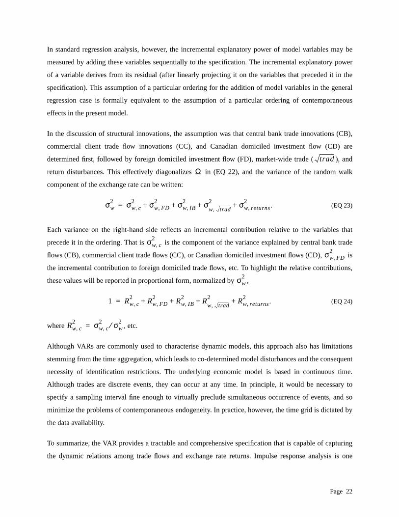
component of the exchange rate can be written:
(EQ 23)
Each variance on the right-hand side reflects an incremental contribution relative to the variable
precede it in the ordering. That is is the component of the variance explained by central bank
flows (CB), commercial client trade flows (CC), or Canadian domiciled investment flows (CD),
the incremental contribution to foreign domiciled trade flows, etc. To highlight the relative contribut
these values will be reported in proportional form, normalized by ,
(EQ 24)
where , etc.
Although VARs are commonly used to characterise dynamic models, this approach also has limit
stemming from the time aggregation, which leads to co-determined model disturbances and the con
necessity of identification restrictions. The underlying economic model is based in continuous
Although trades are discrete events, they can occur at any time. In principle, it would be necess
specify a sampling interval fine enough to virtually preclude simultaneous occurrence of events, a
minimize the problems of contemporaneous endogeneity. In practice, however, the time grid is dicta
the data availability.
To summarize, the VAR provides a tractable and comprehensive specification that is capable of ca
the dynamic relations among trade flows and exchange rate returns. Impulse response analysis
trad
Ω
σw2 σw c,
2 σw FD,2 σw IB,
2 σw trad,2 σw returns,
2.+ + + +=
σw c,2
σw FD,2
σw2
1 Rw c,2
Rw FD,2
Rw IB,2
Rw trad,2
Rw returns,2
.+ + + +=
Rw c,2 σw c,
2 σw2⁄=
Page 22

nges
return
g the
eful in
ssion
in the
non-
he null
in each
st rate
y the
rade
er all
amental
gged
s:
tomer
egated
useful way of characterizing a VAR in the present analysis by constructing the implied price cha
associated with the various types of trade flows. A second characterization of the exchange rate
specification in the VAR involves decomposing the sources of (long-run) return variation amon
variables. Since returns are ultimately driven by changes in information, these analyses are us
attributing information effects and the channels through which they operate.
8. Results
The stationarity of each variable is examined using an Augmented Dickey-Fuller (ADF) test. A regre
of the following form is estimated:
(EQ 25)
where is assumed to be Gaussian white noise, and is the number of lagged terms included
regression is chosen to ensure that the errors are not serially correlated. If , prices are
stationary and have a unit-root. Results are presented in Table 8 and 10. In nearly all cases, t
hypothesis of a unit root is rejected at the 1% significance level.
Tables 9 and 11 presents our estimates of (EQ 1) over the two sample periods. The first regression
table includes only traditional macroeconomic variables that are available at a daily frequency: intere
differentials, crude oil prices, natural gas prices, and non-energy commodity prices. Judging b
model’s explanatory power, the model is clearly inferior to that of a model which includes individual t
flows. More interesting is the predictive power of the regression model that includes order flows. Ov
forecast horizons, and across both sample periods, the order flow regression not only beats the fund
model. but is far superior to the random walk model.
8.1 Inventory-Information Model
The following equation would make it possible to test jointly the effects of contemporaneous and la
customers orders, lagged incoming trade orders, and market-wide order flow on outgoing trade flow
(EQ 26)
The representation extends the model laid out in Section 7.2 naturally to include multi-period cus
orders, and trade-flows that extend beyond two periods. Although individual dealer data dissaggr
∆yt a0 a1yt bt∆yt l– νt+l 1=
f
∑+ +=
νt f
a1 0=
Tit α1cit α+ 21cit 1– … α2 j cit j– α31Tit 1– '… α3kTit k– '+ α41Vt 1– … α4lVt l–++ + +=
Page 23

ble to
ll other
ealer
other
ple in
upport
agged
ll, the
ulation
tructed
nts on
rs and
ot be
struct a
h, or
art with
of the
en in
n in
incoming and outgoing interdealer trades is not available (see Section 6.0), It is still possi
test the model with the net trade flows ( ), defined here as trade between each dealers and a
dealers . If over the course of the day, dealers trade frequently the only position a d
will be left holding at the end of the day is the speculative one. Specifically, traders will pass on to
dealers any undesired position. Consider the adjusted equation to (EQ 26):
(EQ 27)
The model predicts that . OLS estimates of (EQ 27) for each of the 8 dealers in the sam
the spot FX markets are presented in Table 12 and 14. On the whole, results in the spot market s
dealer speculation based on private information. Most of the coefficients are of the correct sign. L
customer orders (CB. CC, CD, FD) and lagged net trade flows are not usually significant. Overa
results confirm the hypothesis of dealer speculation. While there is evidence that this type of spec
does exist, it is short lived (lasting no more that one day). In Tables 13 and 15, F-statistics are cons
to test if the coefficients on contemporaneous central bank trade flows are equal to the coefficie
commercial client trade flows and Canadian domiciled financial institution trade flows. Across deale
in both samples, in virtually all cases the null hypothesis that the coefficients were equal could n
rejected at the 95% significance level.
8.2 VAR Estimation
When we want to take into account all possible relations between variables, it seems sensible to con
model for a vector of time series. In case we also do not know a priori which variable is affecting whic
when it is uncertain which variables are exogenous and which are endogenous, it seems useful to st
the construction of a general time series model for a vector time series.
VARs may also be sensitive to lag length, or in equation (EQ 17). AIC criterion, defined as
(EQ 28)
where is the number of variables in the system, is the sample size, and is an estimate
residual covariance matrix, is employed to determine the lag length of the VAR. The order is chos
order to minimize the criterion. Usually one lag (and sometimes two lags) minimized the AIC criterio
each VARs estimated.
Tit Tit', Tit''
Tit'' Tit Tit'–≡
Tit'' γ1cit γ+ 21cit 1– … γ2 j cit j– γ4Vt γ+ 41Vt 1– … γ4lVt l–++ +=
0 γ1 1–> >
K
AIC K( ) detΩ( )ln 2n2K
T-------------+=
n T Ω
Page 24

casting
sent
at the
variate
test
ber of
to the
sing a
Rs that
either
rdealer
and 3)
rly all
riables.
e price
) are
there is
other
n the
. These
ercial
tion,
As noted
rpreted
ws on
e with
One of the key questions that can be addressed with VARs is how useful some variables are for fore
others. A variable, , is said to Granger-cause another variable, , if the information in past and pre
helps to improve the forecasts of the variable. A block exogeneity test has as its null hypothesis th
lags on one set of variables do not enter the equations for the remaining variables. This is the multi
generalization of Granger-Sims causality tests. The testing procedure used is the Likelihood Ratio
(EQ 29)
where and are the restricted and unrestricted covariance matrices and is the num
observations. This is asymptotically distributed as an distribution with degrees of freedom equal
number of restrictions. is a correction to improve small sample properties. Sims (1980) suggests u
correction equal to the number of variables in each unrestricted equation in the system.
Block exogeneity tests are conducted on aggregate and dealer data, over both samples, using VA
include central bank trade, foreign domiciled trade, interbank trade, market wide trade, and finally
exchange rate returns or implied volatility returns. Three null hypotheses are tested: 1) dealer inte
trade flows are block exogenous; and 2) dealer foreign domiciled trade are block exogenous;
market-wide trade flows ( ) are block exogenous. Results are presented in Table 16. In nea
cases, the null hypotheses are rejected. Therefore all VARs performed will include each of these va
This result suggests that interdealer trade (domestic and foreign) is a necessary requirement in th
discovery process.
The VAR specification described in the previous section (and slight variations in the specification
estimated for all dealers in the sample. The coefficients estimates of the VAR are not reported since
little information to be gained from these estimates. Any one variable in the VAR can affect any
variable in the system both directly, or indirectly through another equation. We instead focus o
impulse response functions and the variance decompositions.
Impulse response functions are computed in each sample subsequent to six different initial shocks
shocks correspond to C$1 million hypothetical spot market sell orders by the central bank, a comm
client, a Canadian domiciled (non-dealer) financial institution, a foreign domiciled financial institu
and a Canadian dealer. The accumulated responses over 20 days are presented in Figures 3 and 4.
above, the long-term cumulative exchange rate returns subsequent to a trade flow shock may be inte
as the information content of the order. There is a clear change in the impact of central bank flo
exchange rate returns from one sample to the next. In the intervention period, central bank trad
x y x
y
T c–( ) Σr( )log Σu( )log–( )
Σr Σu T
χ2
c
i
i
trad
Page 25

lted in a
by the
ent on
ations.
h dealer
elative
flows,
rtion
entages
re not
ly from
th the
ay
bank
rated
riance
the
more
dealers (dealers purchasing Canadian dollars and the central bank selling Canadian dollars) resu
nearly permanent depreciation of the Canadian dollar. This is not true in the replenishment period.
Section 7.3 describes a method for decomposing the long-run exchange rate return variance implied
model into components attributable to the different model variables. These calculations are conting
the identification restrictions governing the contemporaneous influences among the structural innov
The first decomposition uses the same identification as the impulse response calculations. For eac
in the sample, a relative variance decomposition corresponding to (EQ 24) is computed. The r
variance components, the in (EQ 24) are reported in Tables 17-28. Only central bank trade
commercial client trade flows, and foreign domiciled trade flows could explained a significant propo
of the relative variance in exchange rate returns. If exchange rate returns are replaced with perc
change in implied volatility the results are at best poor. In particular, central bank operations we
found to be influential, in either period, in explaining the relative variance in volatility.
9. Conclusion
The results in this papers suggest that central bank trade flows have not been treated very different
other customer orders by dealers in the FX market. In particular, dealers may speculate wi
information implicit in trades directly or indirectly with the central bank, and that this behavour m
impact on the effectiveness of intervention. The paper also illustrates that the impact of central
intervention or replenishment operations is partially determined by market-wide order flows gene
subsequent to intervention operations. For further research, our results (particularly the va
decompositions) also point to the impact of foreign domiciled financial trade flows on prices in
Canadian FX market. The impulse response functions indicate that these flows have become
important recently.
R2s
Page 26

ange
NBER
BIS.
ates?
aper
anada
nk of
nada
er.
. UC
arket.
ook of
References
Amano R. and S. VanNorden (1998). Exchange rates and oil prices.Review of International Economics6,683-694.
Beattie, N. and J.-F. Fillion (1999). An intraday analysis of the effectiveness of foreign exchintervention. Bank of Canada working paper 99-4.
Cao, H. and R. Lyons (1999). Inventory information. UC Berkeley working paper.
Cheung, Y-W. and M. Chinn (1999). Traders, market microstructure and exchange rate dynamics.working paper 7416.
Chiu, P. (2000). Transparency versus constructive ambiguity in foreign exchange intervention.working paper.
Dominguez, K. M. (1993). Does central bank intervention increase the volatility of foreign exchange rNBER working paper 4532.
Dominguez, K. M. (1999) The market microstructure of central bank intervention, NBER working p7337.
D’Souza, C. (2000a). How do FX market intermediaries hedge their exposure to risk? Bank of Cmimeo
D’Souza, C. (2000b). Inventory information and customer-dealer order flows in the FX market. BaCanada mimeo
D’Souza, C. (2000c). The information content of trade flows in the Canadian FX market. Bank of Camimeo
Evans, M. and R. Lyons (1999). Order flow and exchange rate dynamics. UC Berkeley working pap
Evans, M. and R. Lyons (2000). The price impact of currency trades: Implications for interventionBerkeley working paper.
Frankel, J. and K. Froot (1990). Chartists, fundamentalists, and trading in the foreign exchange mAmerican Economic Review80, 181-185.
Frankel, J. and A. Rose (1995). A survey of empirical research on nominal exchange rates. HandbInternational Economics. Volume 3, edited by G. Grossman and K. Rogoff, Elsevier.
Frenkel, J. (1981). Flexible exchange rates, prices and the role of “news”: Lessons from the 1970s.Journalof Political Economy89, 665-705.
Hamilton, J. D. (1994) Time series analysis. Princeton University Press, Princeton.
Hasbrouck, J. (1988). Trades, quotes, inventories and information.Journal of Financial Economics22,229-252.
Hasbrouck, J. (1991a). Measuring the information content of stock trades.Journal of Finance46, 179-207.
Page 27
ation,
saction
NYSE
ederal
ctice
ournal
ics.
aper.
tions.
ut of
oreign
Hasbrouck, J. (1991b). The summary informativeness of stock trades: An econometric investigReview of Financial Studies4, 571-591.
Hasbrouck, J. (1993). Assessing the quality of a security market: A new approach to measuring trancosts,Review of Financial Studies6, 191-212.
Hasbrouck, J. (1995). One security, many market: Determining the contribution to price discovery.Journalof Finance50, 1175-1199.
Hasbrouck, J. (1996). Modelling market microstructure time series.Handbook of Statistics14, 647-692.
Hasbrouck, J. and G. Sofianos (1993). The trades of market makers: An empirical analysis ofspecialists.Journal of Finance48, 1565-1593.
Hung, J. (1995). Intervention strategies and exchange rate volatility: A noise trading perspective. FReserve Bank of New York research paper 9515.
Judge, G., R. Carter, W. Griffiths, H. Lutkepohl and T. Lee (1988). Introduction to the theory and praof econometrics, John Wiley and Sons.
Kim, O. and R. Verrecchia, (1991). Trading volume and price reactions to public announcements. Jof Accounting Research, 29, 302-321.
Krugman, P. (1978). Purchasing power parity and exchange rates: Another look at the evidence.Journal ofInternational Economics8, 397-407.
Lewis, K. (1995). Puzzles in international financial markets. Handbook of International EconomVolume 3, edited by G. Grossman and K. Rogoff. Elsevier.
Lyons, R. (1997). A simultaneous trade model of the foreign exchange hot potato.Journal of InternationalEconomics42, 275-298.
Lyons, R. (1999). The microstructure approach to exchange rates. UC Berkeley working paper.
Madhavan, A. (2000). Market microstructure: A survey. Marshall School of Business, USC working p
Madhavan, A. and S. Smidt (1991). A Bayesian model of intraday specialist pricing.Journal of FinancialEconomics30, 99-134.
Madhavan, A. and S. Smidt (1993). An analysis of changes in specialist inventories and quotaJournal of Finance48, 1595-1628.
Meese, R. and K. Rogoff (1983). Empirical exchange rate models of the seventies. Do they fit osample?Journal of International Economics14, 3-24.
Mussa, M. (1979). Empirical regularities in the behavour of exchange rates and theories of the fexchange market.Carnegie-Rochester Conference Series on Public Policy11, 10-57.
Mussa, M. (1986). The nominal exchange rate regime and the behavour of real exchange rates.Carnegie-Rochester Conference Series on Public Policy26, 117-215.
Page 28

lity,”anada.
aper
Murray, J., M. Zelmer and D. McManus (1997). The effect of intervention on Canadian dollar volatiExchange rates and monetary policy: Proceedings of a conference held by the Bank of COctober 1996: 311-356.
O’Hara, M. (1995). Market microstructure theory. Blackwell Business, Cambridge, MA.
Rogoff, K. (1996). The purchasing power parity puzzle.Journal of Economic Literature34, 647-668.
Schwartz, A. J. (2000). The rise and fall of foreign exchange market intervention. NBER working p7751.
Sims, C. (1980). Macroeconomics and Reality.Econometrica48, 1-49.
Page 29

.00
.98
8.22
8.83
6.52
5.27
9.34
.00
.98
.43
.30
.69
.76
.69
.00
.00
.00
.00
.00
.00
.00
.00
.45
A.1 Tables and Figures
Table 1: Descriptive Statistics ($C millions)
REGIME: INTERVENTION PERIOD: Jan/95-Sep/98 REPLENISHMENT PERIOD:Oct/98-Sep/99
Variables Mean Median Std. Dev. Mean Median Std. Dev.
Aggregate Trading Volumes
Cen. Bank1 27.00 0.00 107.85 0.00 0.00 0
Cen. Bank2 0.00 0.00 0.00 18.94 0.00 37
Total 7722.51 7203.50 3173.54 7778.08 7327.00 239
Interbank 2434.16 2251.30 1232.73 2018.98 1811.95 93
Foreign 3385.70 3179.60 1566.97 3719.79 3561.85 129
Com. Client 1537.04 1462.40 524.66 1639.18 1533.50 63
Can. Dom 338.61 296.00 190.45 381.19 346.40 16
Aggregate Net Trade
Cen. Bank1 -16.18 0.00 110.00 0.00 0.00 0
Cen. Bank2 0.00 0.00 0.00 18.94 0.00 37
Total 130.09 79.20 429.92 37.41 13.40 569
Interbank 15.38 16.40 193.09 -1.99 -6.60 140
Foreign 122.66 100.90 471.79 49.87 30.40 419
Com. Client -16.36 -23.20 232.68 -44.95 -86.45 495
Can. Dom 24.58 14.70 113.60 15.54 9.05 119
Trading Volume, Central Bank Intervention
Dealer 1 8.64 0.00 40.86 0.00 0.00 0
Dealer 2 3.97 0.00 20.92 0.00 0.00 0
Dealer 3 6.29 0.00 28.81 0.00 0.00 0
Dealer 4 4.41 0.00 19.37 0.00 0.00 0
Dealer 5 2.44 0.00 12.57 0.00 0.00 0
Dealer 6 0.41 0.00 3.07 0.00 0.00 0
Dealer 7 0.27 0.00 2.47 0.00 0.00 0
Dealer 8 0.56 0.00 6.36 0.00 0.00 0
Trading Volume, Central Bank Replenishment
Dealer 1 0.00 0.00 0.00 3.39 0.00 11
Page 30

.47
.94
.12
.54
.75
.62
.50
6.64
9.70
0.73
8.55
6.35
0.31
8.30
.26
0.92
2.58
2.62
0.53
5.80
.01
4.10
.12
1.77
1.18
Dealer 2 0.00 0.00 0.00 2.82 0.00 9
Dealer 3 0.00 0.00 0.00 2.38 0.00 8
Dealer 4 0.00 0.00 0.00 3.47 0.00 12
Dealer 5 0.00 0.00 0.00 2.88 0.00 9
Dealer 6 0.00 0.00 0.00 1.13 0.00 4
Dealer 7 0.00 0.00 0.00 1.42 0.00 5
Dealer 8 0.00 0.00 0.00 1.45 0.00 5
Trading Volumes, Total
Dealer 1 1648.24 1508.20 793.34 1979.22 1846.60 71
Dealer 2 1672.14 1547.00 841.79 1113.39 1010.50 60
Dealer 3 1312.88 1175.00 668.85 1720.17 1686.50 64
Dealer 4 1160.66 1086.00 622.49 1200.00 1132.85 51
Dealer 5 979.87 938.00 650.51 892.66 910.00 53
Dealer 6 393.64 343.40 244.64 492.36 475.80 24
Dealer 7 300.67 274.50 152.49 330.49 302.50 14
Dealer 8 254.42 80.00 375.25 49.79 17.50 86
Trading Volumes, Interbank
Dealer 1 507.09 458.07 287.45 478.50 422.86 25
Dealer 2 522.55 469.00 295.59 289.44 248.56 17
Dealer 3 337.89 292.00 215.36 401.10 379.50 19
Dealer 4 421.22 376.90 264.44 358.81 334.60 20
Dealer 5 342.83 318.00 279.42 272.60 249.00 23
Dealer 6 87.67 75.10 61.81 102.31 90.45 62
Dealer 7 112.36 96.70 73.89 116.14 100.80 7
Dealer 8 102.55 0.00 199.65 0.08 0.00 13
Trading Volumes, Foreign Domiciled
Dealer 1 665.49 569.10 397.81 910.07 852.80 40
Dealer 2 869.53 774.00 504.29 525.82 494.00 25
Table 1: Descriptive Statistics ($C millions)
REGIME: INTERVENTION PERIOD: Jan/95-Sep/98 REPLENISHMENT PERIOD:Oct/98-Sep/99
Variables Mean Median Std. Dev. Mean Median Std. Dev.
Page 31

3.29
0.76
8.94
5.91
7.46
.73
9.35
8.10
9.50
1.62
3.76
.26
.96
.81
.14
.74
.00
.97
.93
.10
.22
.35
.00
.00
.00
Dealer 3 578.03 497.00 386.96 929.23 862.50 45
Dealer 4 467.10 408.50 310.98 586.80 561.95 30
Dealer 5 331.51 308.00 270.60 274.58 263.50 20
Dealer 6 230.54 197.60 153.36 318.78 302.75 16
Dealer 7 118.54 102.30 77.98 146.13 132.85 7
Dealer 8 124.96 48.00 179.57 28.37 3.00 72
Trading Volume, Commercial Clients
Dealer 1 375.01 336.10 180.54 472.32 387.30 29
Dealer 2 221.85 196.00 127.40 240.11 194.50 44
Dealer 3 331.37 297.00 166.63 311.24 295.50 11
Dealer 4 223.90 197.30 112.03 185.99 172.60 7
Dealer 5 244.84 212.00 134.87 286.21 264.50 14
Dealer 6 61.69 44.00 60.59 62.80 52.80 46
Dealer 7 63.18 51.30 44.26 64.70 57.05 34
Dealer 8 15.18 7.00 25.15 15.81 6.00 29
Trading Volume, Canadian Domiciled
Dealer 1 92.00 74.00 71.33 114.94 98.45 68
Dealer 2 54.25 36.00 65.92 55.20 46.00 36
Dealer 3 59.30 41.00 59.37 76.22 53.50 79
Dealer 4 44.03 25.00 61.09 64.92 39.00 76
Dealer 5 58.24 43.00 69.26 56.40 46.50 55
Dealer 6 13.33 10.00 21.17 7.34 4.15 11
Dealer 7 6.31 2.70 12.17 2.10 0.00 4
Dealer 8 11.17 3.00 23.91 4.08 0.00 25
Net Trade, Central Bank Intervention
Dealer 1 -6.49 0.00 41.26 0.00 0.00 0
Dealer 2 -2.06 0.00 21.20 0.00 0.00 0
Dealer 3 -3.78 0.00 29.25 0.00 0.00 0
Table 1: Descriptive Statistics ($C millions)
REGIME: INTERVENTION PERIOD: Jan/95-Sep/98 REPLENISHMENT PERIOD:Oct/98-Sep/99
Variables Mean Median Std. Dev. Mean Median Std. Dev.
Page 32

.00
.00
.00
.00
.00
.45
.47
.94
.12
.54
.75
.62
.50
.14
.43
.76
.15
.37
.16
.80
.50
.79
.56
.69
.88
Dealer 4 -1.72 0.00 19.79 0.00 0.00 0
Dealer 5 -1.47 0.00 12.72 0.00 0.00 0
Dealer 6 -0.25 0.00 3.08 0.00 0.00 0
Dealer 7 -0.13 0.00 2.48 0.00 0.00 0
Dealer 8 -0.29 0.00 6.38 0.00 0.00 0
Net Trade, Central Bank Replenishment
Dealer 1 0.00 0.00 0.00 3.39 0.00 11
Dealer 2 0.00 0.00 0.00 2.82 0.00 9
Dealer 3 0.00 0.00 0.00 2.38 0.00 8
Dealer 4 0.00 0.00 0.00 3.47 0.00 12
Dealer 5 0.00 0.00 0.00 2.88 0.00 9
Dealer 6 0.00 0.00 0.00 1.13 0.00 4
Dealer 7 0.00 0.00 0.00 1.42 0.00 5
Dealer 8 0.00 0.00 0.00 1.45 0.00 5
Net Trade, Total
Dealer 1 19.58 21.10 170.67 -9.17 -0.75 188
Dealer 2 14.27 5.00 172.49 26.19 1.00 453
Dealer 3 35.49 22.00 204.41 -3.94 -4.00 154
Dealer 4 21.05 12.70 143.57 8.08 12.50 136
Dealer 5 14.58 8.00 142.32 -2.14 -3.00 147
Dealer 6 9.44 3.70 56.66 10.59 3.60 58
Dealer 7 14.39 8.10 62.95 23.37 15.20 61
Dealer 8 1.30 0.00 75.30 -15.57 0.00 75
Net Trade, Interbank
Dealer 1 -9.29 -8.10 144.04 -11.89 -11.85 138
Dealer 2 -8.48 -8.00 134.46 -0.32 5.00 84
Dealer 3 15.10 10.00 117.75 12.99 3.19 114
Dealer 4 1.46 1.70 115.76 -3.04 -0.05 122
Table 1: Descriptive Statistics ($C millions)
REGIME: INTERVENTION PERIOD: Jan/95-Sep/98 REPLENISHMENT PERIOD:Oct/98-Sep/99
Variables Mean Median Std. Dev. Mean Median Std. Dev.
Page 33
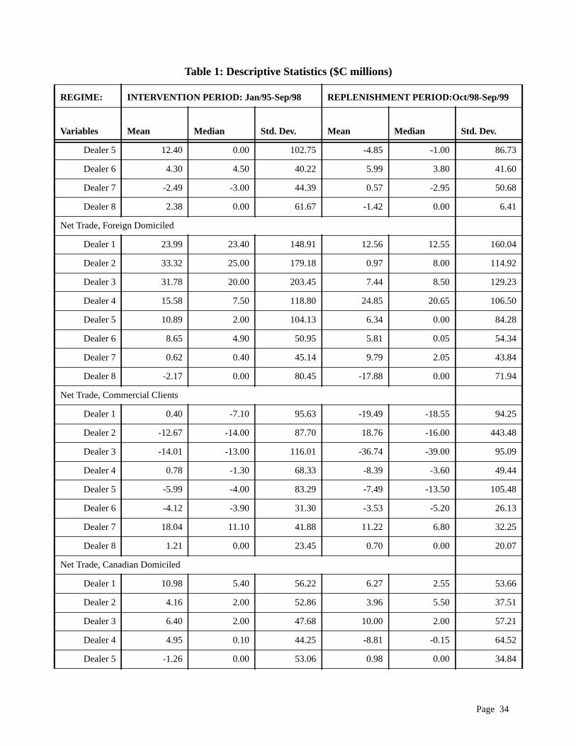
.73
.60
.68
.41
.04
.92
.23
.50
.28
.34
.84
.94
.25
.48
.09
.44
.48
.13
.25
.07
.66
.51
.21
.52
.84
Dealer 5 12.40 0.00 102.75 -4.85 -1.00 86
Dealer 6 4.30 4.50 40.22 5.99 3.80 41
Dealer 7 -2.49 -3.00 44.39 0.57 -2.95 50
Dealer 8 2.38 0.00 61.67 -1.42 0.00 6
Net Trade, Foreign Domiciled
Dealer 1 23.99 23.40 148.91 12.56 12.55 160
Dealer 2 33.32 25.00 179.18 0.97 8.00 114
Dealer 3 31.78 20.00 203.45 7.44 8.50 129
Dealer 4 15.58 7.50 118.80 24.85 20.65 106
Dealer 5 10.89 2.00 104.13 6.34 0.00 84
Dealer 6 8.65 4.90 50.95 5.81 0.05 54
Dealer 7 0.62 0.40 45.14 9.79 2.05 43
Dealer 8 -2.17 0.00 80.45 -17.88 0.00 71
Net Trade, Commercial Clients
Dealer 1 0.40 -7.10 95.63 -19.49 -18.55 94
Dealer 2 -12.67 -14.00 87.70 18.76 -16.00 443
Dealer 3 -14.01 -13.00 116.01 -36.74 -39.00 95
Dealer 4 0.78 -1.30 68.33 -8.39 -3.60 49
Dealer 5 -5.99 -4.00 83.29 -7.49 -13.50 105
Dealer 6 -4.12 -3.90 31.30 -3.53 -5.20 26
Dealer 7 18.04 11.10 41.88 11.22 6.80 32
Dealer 8 1.21 0.00 23.45 0.70 0.00 20
Net Trade, Canadian Domiciled
Dealer 1 10.98 5.40 56.22 6.27 2.55 53
Dealer 2 4.16 2.00 52.86 3.96 5.50 37
Dealer 3 6.40 2.00 47.68 10.00 2.00 57
Dealer 4 4.95 0.10 44.25 -8.81 -0.15 64
Dealer 5 -1.26 0.00 53.06 0.98 0.00 34
Table 1: Descriptive Statistics ($C millions)
REGIME: INTERVENTION PERIOD: Jan/95-Sep/98 REPLENISHMENT PERIOD:Oct/98-Sep/99
Variables Mean Median Std. Dev. Mean Median Std. Dev.
Page 34

.52
.08
.74
Dealer 6 0.85 0.00 20.19 1.20 0.30 10
Dealer 7 -1.66 0.00 12.08 0.37 0.00 4
Dealer 8 0.16 0.00 18.17 1.57 0.00 18
Table 2: Correlations
Sample period: January 2, 1996 - September 30, 1998
Exchange Rate 1.00
Exchange Rate Returns -0.03 1.00
Central Bank Net Trade -0.34 -0.04 1.00
Total Net Trade 0.04 0.01 -0.15 1.00
Interbank Net Trade 0.02 0.01 -0.05 0.19 1.00
Foreign Domiciled Net Trade 0.06 -0.01 -0.39 0.75 -0.11 1.00
Commercial Client Net Trade 0.01 0.05 0.10 0.16 -0.14 -0.34 1.00
Canadian Domicile Net Trade 0.16 0.02 -0.00 0.16 0.02 -0.13 0.05 1.00
Table 1: Descriptive Statistics ($C millions)
REGIME: INTERVENTION PERIOD: Jan/95-Sep/98 REPLENISHMENT PERIOD:Oct/98-Sep/99
Variables Mean Median Std. Dev. Mean Median Std. Dev.
Page 35

Table 3: Correlations
Sample period: October 1, 1998 - September 30, 1999
Exchange Rate 1.00
Exchange Rate Returns 0.11 1.00
Central Bank Net Trade -0.33 -0.01 1.00
Total Net Trade 0.16 -0.08 -0.14 1.00
Interbank Net Trade 0.00 0.01 -0.02 0.18 1.00
Foreign Domiciled Net Trade 0.15 -0.02 -0.36 0.46 -0.11 1.00
Commercial Client Net Trade 0.08 -0.05 0.06 0.73 0.04 -0.19 1.00
Canadian Domicile Net Trade 0.01 -0.10 0.01 -0.07 -0.09 -0.27 -0.06 1.00
Table 4: Correlations
Sample period: January 2, 1996 - September 30, 1999
Exchange Rate 1.00
Exchange Rate Returns 0.04 1.00
Central Bank Net Trade -0.10 -0.02 1.00
Total Net Trade -0.03 -0.03 -0.15 1.00
Interbank Net Trade 0.00 0.01 -0.05 0.19 1.00
Foreign Domiciled Net Trade -0.00 -0.02 -0.38 0.66 -0.11 1.00
Commercial Client Net Trade -0.02 -0.00 0.06 0.43 -0.06 -0.25 1.00
Canadian Domicile Net Trade 0.06 -0.02 -0.02 0.09 -0.00 -0.16 0.01 1.00
Page 36

00
1
5
3
1
0
1
5
3
0
.
ce at
Table 5: Sample period: January 2, 1996 - September 30, 1998
CB NetTrade
TradNetTrade
IB NetTrade
FD NetTrade
CC NetTrade
CD NetTrade
Skewness **1.33 0.08 **-4.08 **1.96 **0.46 **1.22 **-0.42 0.07
Kurtosis **1.30 **3.51 **50.3 **16.9 **3.70 **8.61 **3.67 **8.87
**9191 **34 **247 **52.8 16.74 **48.3 21.84 **32.5
**9167 **243 **169 3.46 20.98 2.42 **25.1 5.80
Auto-correlations 1.00 1.00 1.00 1.00 1.00 1.00 1.00 1.
0.99 0.05 0.26 0.08 0.01 0.16 0.10 -0.0
0.98 0.03 0.14 0.11 0.06 0.07 0.03 0.0
0.97 0.04 0.26 0.03 0.01 0.07 0.04 -0.0
0.96 -0.07 0.09 0.01 0.03 0.00 0.05 0.0
Partial auto-correlations
1.00 1.00 1.00 1.00 1.00 1.00 1.00 1.0
0.99 0.05 0.26 0.08 0.01 0.16 0.10 -0.0
0.07 0.03 0.07 0.10 0.06 0.05 0.02 0.0
-0.01 0.04 0.22 0.02 0.01 0.06 0.04 -0.0
-0.03 -0.08 -0.03 0.00 0.03 -0.02 0.04 0.0
ADF statistic 1.28 **-744 **-57.8 **-72.3 **-153 **-190 **-832 **-47.5
The skewness and kurtosis statistic are normalized so that a value of 0 corresponds to the normal distribution
pertains to the Box-Pierce Q-statistic test for high-order serial correlation in ; * denotes significan
the 95% level; ** denotes significance at the 99% level.
z St Stln∆
Q z∆ 15( )
Qzln∆( )2 15( )
Q z∆ 15( ) z∆
Page 37

00
0
7
3
1
0
0
7
3
1
.
ce at
Table 6: Sample period: October 1, 1998 - September 30, 1999
CB NetTrade
TradNetTrade
IB NetTrade
FD NetTrade
CC NetTrade
CD NetTrade
Skewness 0.12 *0.38 **2.28 **7.59 **-1.63 -0.03 **11.1 -0.18
Kurtosis **-1.18 **1.43 **4.60 **94.2 **11.5 **2.72 **155 **3.84
**1918 12.03 **43.1 8.23 1.82 **70.1 5.27 5.84
**1917 14.41 **24.4 0.13 3.52 14.8 0.07 14.91
Auto-correlations 1.00 1.00 1.00 1.00 1.00 1.00 1.00 1.
0.97 -0.05 0.28 0.07 0.00 0.37 -0.07 0.0
0.94 -0.04 0.09 0.06 0.03 0.24 0.03 -0.0
0.91 0.03 0.00 0.12 -0.05 0.19 0.04 0.0
0.89 0.20 0.09 0.01 -0.00 0.12 0.07 -0.0
Partial auto-correlations
1.00 1.00 1.00 1.00 1.00 1.00 1.00 1.0
0.97 -0.05 0.28 0.07 0.00 0.37 -0.07 0.0
0.02 -0.04 0.01 0.05 0.03 0.11 0.02 -0.0
-0.01 0.02 -0.03 0.11 -0.05 0.08 0.04 0.0
0.00 0.00 0.22 -0.00 -0.00 0.01 0.07 -0.0
ADF statistic **-5.13 **-331 **-82.4 **-90.1 **-563 **-67.8 **-454 **-235
The skewness and kurtosis statistic are normalized so that a value of 0 corresponds to the normal distribution
pertains to the Box-Pierce Q-statistic test for high-order serial correlation in ; * denotes significan
the 95% level; ** denotes significance at the 99% level.
z St Stln∆
Q z∆ 10( )
Qzln∆( )2 10( )
Q z∆ 15( ) z∆
Page 38

.00
0
2
1
0
0
0
2
1
0
.
nce at
Table 7: Sample period: January 2, 1996 - September 30, 1999
CB NetTrade
TradNetTrade
IB NetTrade
FD NetTrade
CC NetTrade
CD NetTrade
Skewness **0.47 **0.30 **-4.50 **4.33 *0.17 **1.02 **9.72 0.00
Kurtosis **-1.12 **2.96 **61.8 **54.7 **4.94 **7.93 **205 **7.50
**11781 **40.7 **442 **67.2 21.16 **101 18.73 *28.3
**11779 **373 **238 0.51 20.34 8.19 0.18 9.03
Auto-correlations 1.00 1.00 1.00 1.00 1.00 1.00 1.00 1
0.99 0.00 0.28 0.09 0.01 0.21 0.00 -0.0
0.99 0.01 0.16 0.10 0.06 0.11 0.03 0.0
0.98 0.04 0.27 0.08 -0.00 0.10 0.04 -0.0
0.98 -0.06 0.12 0.02 0.03 0.03 0.06 0.0
Partial auto-correlations
1.00 1.00 1.00 1.00 1.00 1.00 1.00 1.0
0.99 0.00 0.28 0.09 0.01 0.21 0.00 -0.0
-0.00 0.01 0.08 0.09 0.06 0.07 0.03 0.0
-0.01 0.04 0.22 0.06 -0.01 0.07 0.04 -0.0
-0.03 -0.06 -0.01 0.02 0.02 -0.01 0.06 0.0
ADF statistic -1.90 **-590 **-100 **-108 **-254 **-370 **-436 **-132
The skewness and kurtosis statistic are normalized so that a value of 0 corresponds to the normal distribution
pertains to the Box-Pierce Q-statistic test for high-order serial correlation in ; * denotes significa
the 95% level; ** denotes significance at the 99% level.
z St Stln∆
Q z∆ 20( )
Qzln∆( )2 20( )
Q z∆ 15( ) z∆
Page 39
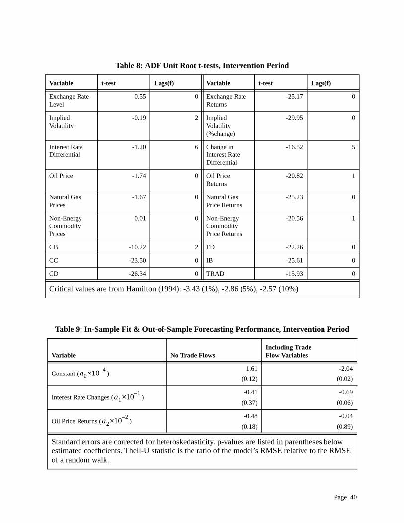
lowSE
Table 8: ADF Unit Root t-tests, Intervention Period
Variable t-test Lags(f) Variable t-test Lags(f)
Exchange RateLevel
0.55 0 Exchange RateReturns
-25.17 0
ImpliedVolatility
-0.19 2 ImpliedVolatility(%change)
-29.95 0
Interest RateDifferential
-1.20 6 Change inInterest RateDifferential
-16.52 5
Oil Price -1.74 0 Oil PriceReturns
-20.82 1
Natural GasPrices
-1.67 0 Natural GasPrice Returns
-25.23 0
Non-EnergyCommodityPrices
0.01 0 Non-EnergyCommodityPrice Returns
-20.56 1
CB -10.22 2 FD -22.26 0
CC -23.50 0 IB -25.61 0
CD -26.34 0 TRAD -15.93 0
Critical values are from Hamilton (1994): -3.43 (1%), -2.86 (5%), -2.57 (10%)
Table 9: In-Sample Fit & Out-of-Sample Forecasting Performance, Intervention Period
Variable No Trade FlowsIncluding TradeFlow Variables
Constant ( )1.61
(0.12)
-2.04
(0.02)
Interest Rate Changes ( )-0.41
(0.37)
-0.69
(0.06)
Oil Price Returns ( )-0.48
(0.18)
-0.04
(0.89)
Standard errors are corrected for heteroskedasticity. p-values are listed in parentheses beestimated coefficients. Theil-U statistic is the ratio of the model’s RMSE relative to the RMof a random walk.
a04–×10
a11–×10
a22–×10
Page 40
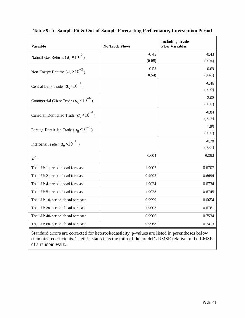
lowSE
Natural Gas Returns ( )-0.45
(0.08)
-0.43
(0.04)
Non-Energy Returns ( )-0.58
(0.54)
-0.69
(0.40)
Central Bank Trade ( )-6.46
(0.00)
Commercial Client Trade ( )-2.02
(0.00)
Canadian Domiciled Trade ( )-0.84
(0.29)
Foreign Domiciled Trade ( )1.89
(0.00)
Interbank Trade ( )-0.78
(0.34)
0.004 0.352
Theil-U: 1-period ahead forecast 1.0007 0.6707
Theil-U: 2-period ahead forecast 0.9995 0.6694
Theil-U: 4-period ahead forecast 1.0024 0.6734
Theil-U: 5-period ahead forecast 1.0028 0.6745
Theil-U: 10-period ahead forecast 0.9999 0.6654
Theil-U: 20-period ahead forecast 1.0003 0.6761
Theil-U: 40-period ahead forecast 0.9906 0.7534
Theil-U: 60-period ahead forecast 0.9968 0.7413
Table 9: In-Sample Fit & Out-of-Sample Forecasting Performance, Intervention Period
Variable No Trade FlowsIncluding TradeFlow Variables
Standard errors are corrected for heteroskedasticity. p-values are listed in parentheses beestimated coefficients. Theil-U statistic is the ratio of the model’s RMSE relative to the RMof a random walk.
a32–×10
a42–×10
a56–×10
a66–×10
a76–×10
a86–×10
a96–×10
R2
Page 41

lowSE
Table 10: ADF Unit Root t-tests, Replenishment Period
Variable t-test Lags(f) Variable t-test Lags(f)
Exchange RateLevel
-1.54 0 Exchange RateReturns
-16.42 0
ImpliedVolatility
-2.30 0 ImpliedVolatility(%change)
-17.50 0
Interest RateDifferential
-2.86 1 Change inInterest RateDifferential
-11.34 5
Oil Price -0.82 0 Oil PriceReturns
-15.69 0
Natural GasPrices
-1.28 0 Natural GasPrice Returns
-15.61 0
Non-EnergyCommodityPrices
-0.80 1 Non-EnergyCommodityPrice Returns
-13.16 0
CB -10.22 0 FD -10.58 0
CC -16.94 0 IB -16.09 0
CD -15.98 0 TRAD -15.93 0
Critical values are from Hamilton (1994): -3.43 (1%), -2.86 (5%), -2.57 (10%)
Table 11: In-Sample Fit & Out-of-Sample Forecasting Performance, Replenishment Period
Variable No Trade FlowsIncluding TradeFlow Variables
Constant ( )-0.82
(0.74)
4.27
(0.07)
Interest Rate Changes ( )-0.02
(0.29)
-1.22
(0.31)
Oil Price Returns ( )-2.00
(0.08)
-0.84
(0.34)
Standard errors are corrected for heteroskedasticity. p-values are listed in parentheses beestimated coefficients. Theil-U statistic is the ratio of the model’s RMSE relative to the RMof a random walk.
a04–×10
a11–×10
a22–×10
Page 42

lowSE
Natural Gas Returns ( )-0.10
(0.24)
-0.92
(0.13)
Non-Energy Returns ( )-4.54
(0.08)
-0.01
(0.98)
Central Bank Trade ( )-4.09
(0.00)
Commercial Client Trade ( )-1.12
(0.00)
Canadian Domiciled Trade ( )-0.10
(0.64)
Foreign Domiciled Trade ( )3.10
(0.00)
Interbank Trade ( )-0.83
(0.66)
0.026 0.395
Theil-U: 1-period ahead forecast 1.0199 0.5481
Theil-U: 2-period ahead forecast 1.0152 0.5482
Theil-U: 4-period ahead forecast 1.0045 0.5760
Theil-U: 5-period ahead forecast 1.0055 0.5790
Theil-U: 10-period ahead forecast 1.0030 0.6114
Theil-U: 20-period ahead forecast 1.0280 0.5817
Theil-U: 40-period ahead forecast 1.0048 0.5884
Theil-U: 60-period ahead forecast 0.9607 0.5898
Table 11: In-Sample Fit & Out-of-Sample Forecasting Performance, Replenishment Period
Variable No Trade FlowsIncluding TradeFlow Variables
Standard errors are corrected for heteroskedasticity. p-values are listed in parentheses beestimated coefficients. Theil-U statistic is the ratio of the model’s RMSE relative to the RMof a random walk.
a32–×10
a42–×10
a56–×10
a66–×10
a76–×10
a86–×10
a96–×10
R2
Page 43
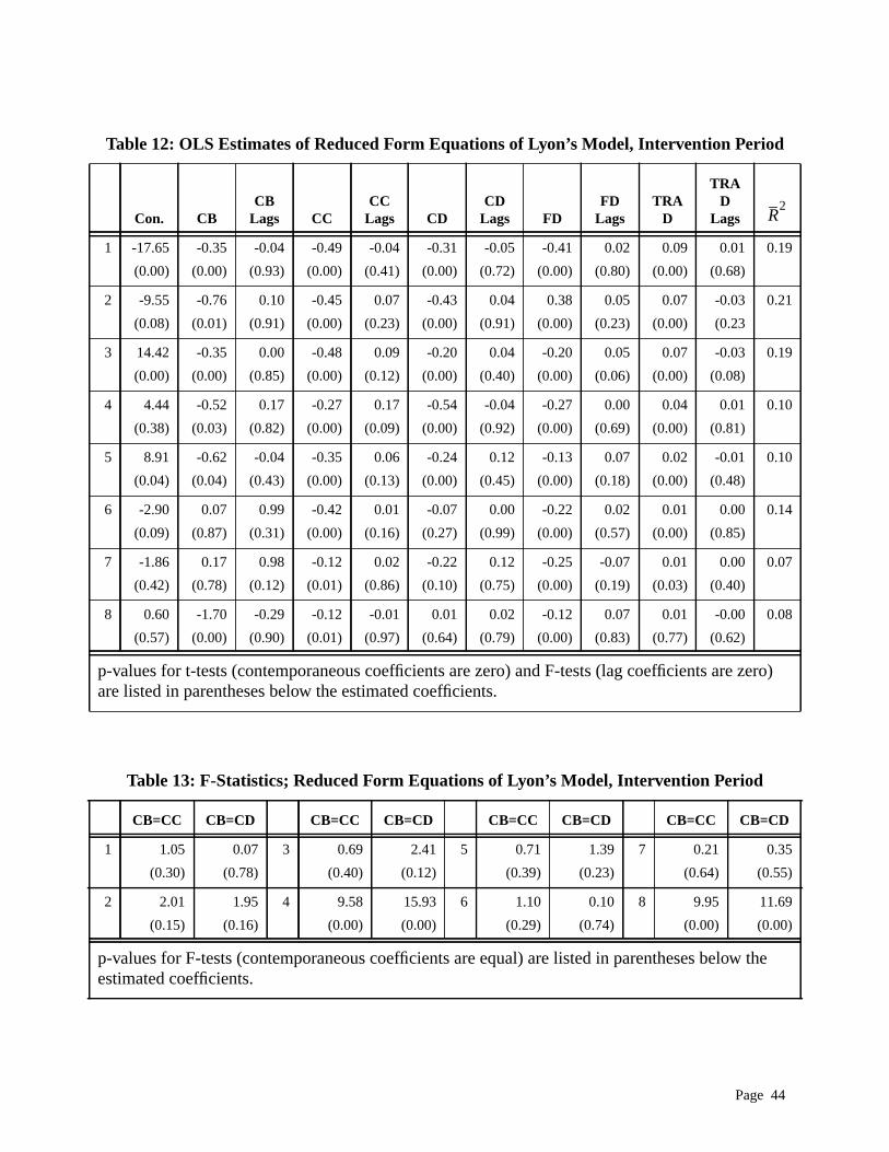
zero)
w the
Table 12: OLS Estimates of Reduced Form Equations of Lyon’s Model, Intervention Period
Con. CBCB
Lags CCCC
Lags CDCD
Lags FDFD
LagsTRA
D
TRAD
Lags
1 -17.65
(0.00)
-0.35
(0.00)
-0.04
(0.93)
-0.49
(0.00)
-0.04
(0.41)
-0.31
(0.00)
-0.05
(0.72)
-0.41
(0.00)
0.02
(0.80)
0.09
(0.00)
0.01
(0.68)
0.19
2 -9.55
(0.08)
-0.76
(0.01)
0.10
(0.91)
-0.45
(0.00)
0.07
(0.23)
-0.43
(0.00)
0.04
(0.91)
0.38
(0.00)
0.05
(0.23)
0.07
(0.00)
-0.03
(0.23
0.21
3 14.42
(0.00)
-0.35
(0.00)
0.00
(0.85)
-0.48
(0.00)
0.09
(0.12)
-0.20
(0.00)
0.04
(0.40)
-0.20
(0.00)
0.05
(0.06)
0.07
(0.00)
-0.03
(0.08)
0.19
4 4.44
(0.38)
-0.52
(0.03)
0.17
(0.82)
-0.27
(0.00)
0.17
(0.09)
-0.54
(0.00)
-0.04
(0.92)
-0.27
(0.00)
0.00
(0.69)
0.04
(0.00)
0.01
(0.81)
0.10
5 8.91
(0.04)
-0.62
(0.04)
-0.04
(0.43)
-0.35
(0.00)
0.06
(0.13)
-0.24
(0.00)
0.12
(0.45)
-0.13
(0.00)
0.07
(0.18)
0.02
(0.00)
-0.01
(0.48)
0.10
6 -2.90
(0.09)
0.07
(0.87)
0.99
(0.31)
-0.42
(0.00)
0.01
(0.16)
-0.07
(0.27)
0.00
(0.99)
-0.22
(0.00)
0.02
(0.57)
0.01
(0.00)
0.00
(0.85)
0.14
7 -1.86
(0.42)
0.17
(0.78)
0.98
(0.12)
-0.12
(0.01)
0.02
(0.86)
-0.22
(0.10)
0.12
(0.75)
-0.25
(0.00)
-0.07
(0.19)
0.01
(0.03)
0.00
(0.40)
0.07
8 0.60
(0.57)
-1.70
(0.00)
-0.29
(0.90)
-0.12
(0.01)
-0.01
(0.97)
0.01
(0.64)
0.02
(0.79)
-0.12
(0.00)
0.07
(0.83)
0.01
(0.77)
-0.00
(0.62)
0.08
p-values for t-tests (contemporaneous coefficients are zero) and F-tests (lag coefficients areare listed in parentheses below the estimated coefficients.
Table 13: F-Statistics; Reduced Form Equations of Lyon’s Model, Intervention Period
CB=CC CB=CD CB=CC CB=CD CB=CC CB=CD CB=CC CB=CD
1 1.05
(0.30)
0.07
(0.78)
3 0.69
(0.40)
2.41
(0.12)
5 0.71
(0.39)
1.39
(0.23)
7 0.21
(0.64)
0.35
(0.55)
2 2.01
(0.15)
1.95
(0.16)
4 9.58
(0.00)
15.93
(0.00)
6 1.10
(0.29)
0.10
(0.74)
8 9.95
(0.00)
11.69
(0.00)
p-values for F-tests (contemporaneous coefficients are equal) are listed in parentheses beloestimated coefficients.
R2
Page 44

d
zero)
w the
Table 14: OLS Estimates of Reduced Form Equations of Lyon’s Model, Replenishment Perio
Con. CBCB
Lags CCCC
Lags CDCD
Lags FDFD
LagsTRA
D
TRAD
Lags
1 -6.34
(0.55)
1.18
(0.11)
0.83
(0.49)
-0.12
(0.20)
0.09
(0.29)
-0.72
(0.00)
0.77
(0.00)
-0.26
(0.00)
0.03
(0.76)
0.03
(0.05)
-0.02
(0.47)
0.12
2 0.94
(0.87)
-0.38
(0.49)
0.12
(0.20)
-0.01
(0.69)
-0.28
(0.01)
-0.28
(0.05)
-0.11
(0.78)
-0.15
(0.01)
0.11
(0.12)
0.01
(0.72)
0.01
(0.89)
0.13
3 3.64
(0.69)
-1.06
(0.17)
1.82
(0.21)
-0.42
(0.00)
0.07
(0.76)
-0.55
(0.00)
0.06
(0.89)
-0.13
(0.02)
0.03
(0.58)
0.02
(0.15)
-0.05
(0.53)
0.15
4 -5.67
(0.53)
0.58
(0.37)
0.40
(0.68)
-0.26
(0.10)
-0.05
(0.04)
-0.53
(0.00)
0.17
(0.05)
-0.30
(0.00)
-0.01
(0.96)
0.02
(0.20)
0.02
(0.46)
0.12
5 -4.36
(0.49)
-0.31
(0.60)
-0.64
(0.73)
-0.10
(0.07)
-0.06
(0.53)
-0.31
(0.06)
-0.19
(0.17)
0.06
(0.37)
0.01
(0.89)
0.02
(0.05)
0.00
(0.82)
0.02
6 6.56
(0.49)
-0.73
(0.18)
0.01
(0.93)
-0.50
(0.00)
--0.01
(0.29)
-0.67
(0.01)
-0.28
(0.33)
-0.17
(0.00)
0.04
(0.56)
0.00
(0.59)
0.01
(0.52)
0.09
7 7.85
(0.02)
-0.10
(0.82)
-0.43
(0.84)
-0.24
(0.02)
-0.06
(0.87)
-0.13
(0.87)
0.13
(0.15)
-0.23
(0.00)
0.03
(0.93)
0.00
(0.70)
-0.01
(0.32)
0.02
8 0.09
(0.72)
-1.00
(0.00)
-0.00
(0.98)
-0.00
(0.82)
0.01
(0.39)
-0.01
(0.48)
-0.02
(0.35)
0.00
(0.89)
0.00
(0.93)
0.00
(0.42)
-0.00
(0.92)
0.73
p-values for t-tests (contemporaneous coefficients are zero) and F-tests (lag coefficients areare listed in parentheses below the estimated coefficients.
Table 15: F-Statistics; Reduced Form Equations of Lyon’s Model, Replenishment Period
CB=CC CB=CD CB=CC CB=CD CB=CC CB=CD CB=CC CB=CD
1 2.97
(0.08)
6.36
(0.01)
3 0.66
(0.41)
0.41
(0.51)
5 0.12
(0.72)
0.00
(0.99)
7 0.05
(0.80)
0.00
(0.97)
2 0.46
(0.49)
0.03
(0.84)
4 1.58
(0.20)
2.88
(0.09)
6 0.16
(0.68)
0.01
(0.91)
8 585.14
(0.00)
590.34
(0.00)
p-values for F-tests (contemporaneous coefficients are equal) are listed in parentheses beloestimated coefficients.
R2
Page 45

ber ofity at
Table 16: Significance of Block Exogeneity Tests
Exchange Rate Returns Implied Volatility
FD IB FD IB
Sample Sample Sample Sample Sample Sample
1 2 1 2 1 2 1 2 1 2 1 2
Aggregate * * * * * * * * * * * *
Dealer 1 * * * * * * * * * * * *
Dealer 2 * * * * * * * * * *
Dealer 3 * * * * * * * * * * *
Dealer 4 * * * * * * * * * * * *
Dealer 5 * * * * * * * * * * * *
Dealer 6 * * * * * * * * * * *
Dealer 7 * * * * * * * * * * *
Dealer 8 * * * * * * * * * *
Likelihood ratio test statistics have a distribution with degrees of freedom equal to the numrestrictions placed on the VAR. * indicates a rejection of the null hypothesis of block Exogenethe 95% level.
TRAD TRAD
χ2
Page 46
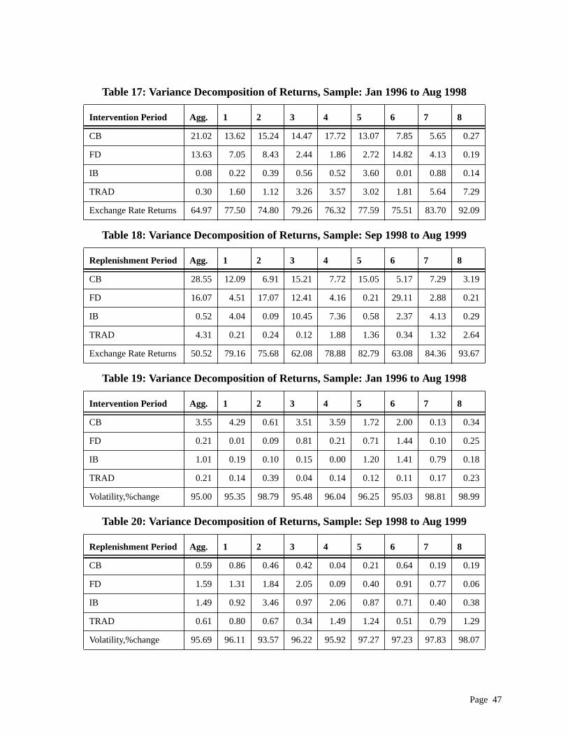
Table 17: Variance Decomposition of Returns, Sample: Jan 1996 to Aug 1998
Intervention Period Agg. 1 2 3 4 5 6 7 8
CB 21.02 13.62 15.24 14.47 17.72 13.07 7.85 5.65 0.27
FD 13.63 7.05 8.43 2.44 1.86 2.72 14.82 4.13 0.19
IB 0.08 0.22 0.39 0.56 0.52 3.60 0.01 0.88 0.14
TRAD 0.30 1.60 1.12 3.26 3.57 3.02 1.81 5.64 7.29
Exchange Rate Returns 64.97 77.50 74.80 79.26 76.32 77.59 75.51 83.70 92.09
Table 18: Variance Decomposition of Returns, Sample: Sep 1998 to Aug 1999
Replenishment Period Agg. 1 2 3 4 5 6 7 8
CB 28.55 12.09 6.91 15.21 7.72 15.05 5.17 7.29 3.19
FD 16.07 4.51 17.07 12.41 4.16 0.21 29.11 2.88 0.21
IB 0.52 4.04 0.09 10.45 7.36 0.58 2.37 4.13 0.29
TRAD 4.31 0.21 0.24 0.12 1.88 1.36 0.34 1.32 2.64
Exchange Rate Returns 50.52 79.16 75.68 62.08 78.88 82.79 63.08 84.36 93.67
Table 19: Variance Decomposition of Returns, Sample: Jan 1996 to Aug 1998
Intervention Period Agg. 1 2 3 4 5 6 7 8
CB 3.55 4.29 0.61 3.51 3.59 1.72 2.00 0.13 0.34
FD 0.21 0.01 0.09 0.81 0.21 0.71 1.44 0.10 0.25
IB 1.01 0.19 0.10 0.15 0.00 1.20 1.41 0.79 0.18
TRAD 0.21 0.14 0.39 0.04 0.14 0.12 0.11 0.17 0.23
Volatility,%change 95.00 95.35 98.79 95.48 96.04 96.25 95.03 98.81 98.99
Table 20: Variance Decomposition of Returns, Sample: Sep 1998 to Aug 1999
Replenishment Period Agg. 1 2 3 4 5 6 7 8
CB 0.59 0.86 0.46 0.42 0.04 0.21 0.64 0.19 0.19
FD 1.59 1.31 1.84 2.05 0.09 0.40 0.91 0.77 0.06
IB 1.49 0.92 3.46 0.97 2.06 0.87 0.71 0.40 0.38
TRAD 0.61 0.80 0.67 0.34 1.49 1.24 0.51 0.79 1.29
Volatility,%change 95.69 96.11 93.57 96.22 95.92 97.27 97.23 97.83 98.07
Page 47

Table 21: Variance Decomposition of Returns, Sample: Jan 1996 to Aug 1998
Intervention Period Agg. 1 2 3 4 5 6 7 8
CC 9.73 5.34 1.21 0.38 3.52 2.47 1.15 1.22 0.19
FD 19.67 10.13 13.08 5.23 2.29 3.01 20.22 3.82 0.11
IB 0.04 0.53 0.83 0.63 1.43 3.39 0.07 0.79 0.16
TRAD 0.36 2.76 1.03 3.73 6.58 4.88 1.98 6.75 7.27
Exchange Rate Returns 70.15 81.22 83.84 90.01 86.17 86.25 76.57 87.41 92.25
Table 22: Variance Decomposition of Returns, Sample: Sep 1998 to Aug 1999
Replenishment Period Agg. 1 2 3 4 5 6 7 8
CC 4.70 5.55 1.26 1.72 0.83 3.56 8.40 4.72 0.74
FD 24.61 4.85 19.10 15.95 4.30 8.25 25.18 3.44 0.15
IB 0.40 4.77 0.16 11.36 7.03 0.63 1.84 3.15 3.48
TRAD 3.84 1.24 0.35 0.14 2.76 2.99 0.17 1.87 2.68
Exchange Rate Returns 66.44 83.59 79.12 70.81 85.08 92.54 64.39 86.89 92.95
Table 23: Variance Decomposition of Returns, Sample: Jan 1996 to Aug 1998
Intervention Period Agg. 1 2 3 4 5 6 7 8
CC 0.10 0.79 0.13 0.01 0.42 0.03 1.46 0.19 0.08
FD 1.76 0.53 0.12 1.35 0.48 0.88 3.06 0.14 0.23
IB 0.57 0.07 0.13 0.07 0.05 1.34 0.67 0.83 0.15
TRAD 0.67 0.21 0.32 0.08 0.10 0.15 0.09 0.13 0.23
Volatility,%change 96.88 98.38 99.29 98.48 98.95 95.59 94.71 98.69 99.30
Table 24: Variance Decomposition of Returns, Sample: Sep 1998 to Aug 1999
Replenishment Period Agg. 1 2 3 4 5 6 7 8
CC 0.10 0.06 0.57 2.33 1.73 0.22 1.11 0.67 0.51
FD 1.72 1.36 1.83 1.40 0.37 0.41 0.62 0.70 0.11
IB 1.53 0.90 2.74 0.62 1.72 0.77 1.09 0.30 0.43
TRAD 1.15 0.77 0.73 0.41 1.50 1.28 0.74 0.76 1.34
Volatility,%change 95.47 96.92 94.11 95.23 94.66 97.31 96.43 97.55 97.60
Page 48

Table 25: Variance Decomposition of Returns, Sample: Jan 1996 to Aug 1998
Intervention Period Agg. 1 2 3 4 5 6 7 8
CD 0.67 0.06 0.63 0.15 2.31 0.56 1.35 0.28 0.00
FD 26.81 13.20 13.69 5.98 2.84 3.95 20.46 4.11 0.21
IB 0.03 0.11 0.85 0.92 1.61 4.63 0.02 0.84 0.18
TRAD 1.33 1.44 0.99 3.11 6.35 3.75 2.01 6.12 7.28
Exchange Rate Returns 71.14 85.22 83.84 89.22 86.89 87.12 76.16 88.64 92.31
Table 26: Variance Decomposition of Returns, Sample: Sep 1998 to Aug 1999
Replenishment Period Agg. 1 2 3 4 5 6 7 8
CD 2.71 2.99 0.58 2.97 1.34 3.41 1.65 0.18 2.61
FD 26.46 8.02 20.27 15.45 4.94 0.41 30.73 3.81 0.20
IB 0.24 3.34 0.22 10.38 6.45 1.20 2.14 3.97 3.24
TRAD 4.71 0.31 0.20 0.09 2.48 1.67 0.22 1.57 2.89
Exchange Rate Returns 65.89 85.34 78.72 71.10 84.79 93.29 65.24 90.76 91.07
Table 27: Variance Decomposition of Returns, Sample: Jan 1996 to Aug 1998
Intervention Period Agg. 1 2 3 4 5 6 7 8
CD 0.30 0.90 0.04 0.32 0.16 0.03 0.24 0.12 0.01
FD 1.33 0.51 0.13 1.21 0.54 0.89 2.45 0.11 0.28
IB 0.79 0.05 0.08 0.13 0.03 1.33 1.51 0.78 0.14
TRAD 0.41 0.20 0.37 0.05 0.11 0.13 0.13 0.19 0.23
Volatility,%change 97.14 98.34 99.36 98.27 99.16 97.61 95.66 98.81 99.33
Table 28: Variance Decomposition of Returns, Sample: Sep 1998 to Aug 1999
Replenishment Period Agg. 1 2 3 4 5 6 7 8
CD 0.36 0.03 0.43 0.76 0.42 0.07 5.39 0.71 0.65
FD 1.95 1.38 2.28 1.34 1.41 0.44 1.39 0.74 0.65
IB 1.42 0.79 3.41 1.17 2.01 0.76 0.46 0.31 0.43
TRAD 0.49 0.83 0.63 0.37 1.34 1.22 0.31 0.77 1.41
Volatility,%change 95.77 96.96 93.24 96.35 93.80 97.49 92.49 97.47 97.45
Page 49

1
FIGURE 2. Cumulative Change in Returns in Response to Aggregate Shocks, SampleCB
1 3 5 7 9-0.020
-0.015
-0.010
-0.005
0.000
0.005
0.010
0.015
0.020
CC
1 3 5 7 9-0.020
-0.015
-0.010
-0.005
0.000
0.005
0.010
0.015
0.020
CD
1 3 5 7 9-0.020
-0.015
-0.010
-0.005
0.000
0.005
0.010
0.015
0.020
IB
1 3 5 7 9-0.020
-0.015
-0.010
-0.005
0.000
0.005
0.010
0.015
0.020
FD
1 3 5 7 9-0.020
-0.015
-0.010
-0.005
0.000
0.005
0.010
0.015
0.020
TRAD
1 3 5 7 9-0.020
-0.015
-0.010
-0.005
0.000
0.005
0.010
0.015
0.020
Page 50
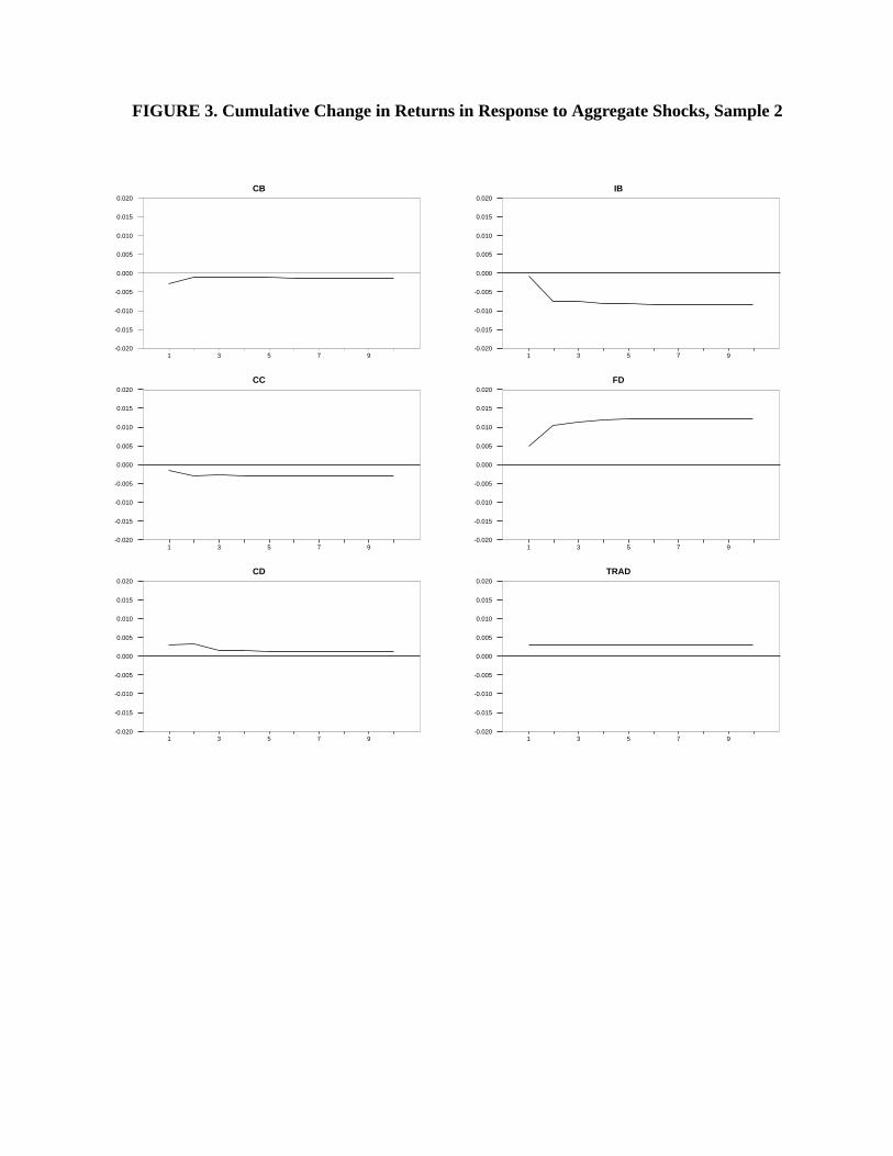
2
FIGURE 3. Cumulative Change in Returns in Response to Aggregate Shocks, SampleCB
1 3 5 7 9-0.020
-0.015
-0.010
-0.005
0.000
0.005
0.010
0.015
0.020
CC
1 3 5 7 9-0.020
-0.015
-0.010
-0.005
0.000
0.005
0.010
0.015
0.020
CD
1 3 5 7 9-0.020
-0.015
-0.010
-0.005
0.000
0.005
0.010
0.015
0.020
IB
1 3 5 7 9-0.020
-0.015
-0.010
-0.005
0.000
0.005
0.010
0.015
0.020
FD
1 3 5 7 9-0.020
-0.015
-0.010
-0.005
0.000
0.005
0.010
0.015
0.020
TRAD
1 3 5 7 9-0.020
-0.015
-0.010
-0.005
0.000
0.005
0.010
0.015
0.020