Magnetic Flux Leakage Device for Evaluation of Prestressed ...

A Magnetic Flux Leakage NDE System
for CANDUR© Feeder Pipes
by
Thomas Don Mak
A thesis submitted to the
Department of Physics, Engineering Physics & Astronomy
in conformity with the requirements for
the degree of Master of Applied Science
Queen’s University
Kingston, Ontario, Canada
March 2010
Copyright c© Thomas Don Mak, 2010

Abstract
This work examines the application of different magnetic flux leakage (MFL) inspec-
tion concepts to the non destructive evaluation (NDE) of residual (elastic) stresses in
CANDU R© reactor feeder pipes. The stress sensitivity of three MFL inspection tech-
niques was examined with flat plate samples, with stress-induced magnetic anisotropy
(SMA) demonstrating the greatest stress sensitivity. A prototype SMA testing sys-
tem was developed to apply magnetic NDE to feeders. The system consists of a flux
controller that incorporates feedback from a wire coil and a Hall sensor (FCV2), and
a magnetic anisotropy prototype (MAP) probe. The combination of FCV2 and the
MAP probe was shown to provide SMA measurements on feeder pipe samples and
predict stresses from SMA measurements with a mean accuracy of ±38 MPa.
i
Acknowledgments
First and foremost I would like to thank my supervisor, Dr. Lynann Clapham, for
presenting me with this wonderful opportunity. Her guidance and expertise were
greatly appreciated.
This work would have been far less interesting and enjoyable without the assistance
of Dr. Steven White. He acted as a teacher from the moment I began working under
him as a summer student in 2006, and he provided invaluable assistance in all aspects
of this project from its conception, from theory to design, data acquisition and signal
processing.
I would also like to thank all members of the AECL Inspection Monitoring and
Dynamics Branch, in particular Helene Hebert. She helped organize meetings with
AECL and provided helpful advice and encouragement.
Thanks are due to Dirk Bouma, who was consulted frequently during the design
of the first flux control system (FCV1), as well as Gary Contant and Chuck Hearns
for their help and supervision in the machine shop. I also thank Pat Wayman for all
her help during all phases of this project.
Several students provided valuable assistance: Ben Lucht helped with LATEX and
MATLAB R©, and Davin Young spent many hours in the machine shop building probe
components.
ii

Table of Contents
Abstract i
Acknowledgments ii
Table of Contents iii
List of Tables v
List of Figures vi
Chapter 1:
Introduction . . . . . . . . . . . . . . . . . . . . . . . . . . 1
1.1 CANDUR© Feeder Pipes . . . . . . . . . . . . . . . . . . . . . . . . . 2
1.2 A Brief Introduction to Magnetic Circuits and Magnetic Flux Leakage
Inspection . . . . . . . . . . . . . . . . . . . . . . . . . . . . . . . . . 5
1.3 Thesis Scope and Objectives . . . . . . . . . . . . . . . . . . . . . . . 7
1.4 Organization of Thesis . . . . . . . . . . . . . . . . . . . . . . . . . . 8
Chapter 2:
Theory and Background . . . . . . . . . . . . . . . . . . . 10
2.1 Stress and Strain . . . . . . . . . . . . . . . . . . . . . . . . . . . . . 10
iii

2.2 Maxwell’s Equations and The Quasi-Static Case . . . . . . . . . . . . 15
2.3 Magnetic Materials . . . . . . . . . . . . . . . . . . . . . . . . . . . . 16
2.4 Magnetic Methods of Stress Measurement . . . . . . . . . . . . . . . 29
Chapter 3:
Flux Control Systems . . . . . . . . . . . . . . . . . . . . 39
3.1 Negative Feedback Control and Operational Amplifiers . . . . . . . . 40
3.2 Magnetic Flux Transducers . . . . . . . . . . . . . . . . . . . . . . . 42
3.3 Component Selection . . . . . . . . . . . . . . . . . . . . . . . . . . . 47
3.4 White’s Flux Control System (FCS) . . . . . . . . . . . . . . . . . . . 49
3.5 Flux Control Version 1 (FCV1): Hall Sensor Feedback . . . . . . . . 51
3.6 Flux Control Version 2 (FCV2): Hall Sensor and Coil Feedback in
Combination . . . . . . . . . . . . . . . . . . . . . . . . . . . . . . . . 60
Chapter 4:
Magnetic Stress Detectors . . . . . . . . . . . . . . . . . . 67
4.1 Test Sample and the Single Axis Stress Rig (SASR) . . . . . . . . . . 69
4.2 Detectors, Data Acquisition and Data Analysis . . . . . . . . . . . . 72
4.3 Experimental Procedures for Testing and Comparison of the Probe
Systems . . . . . . . . . . . . . . . . . . . . . . . . . . . . . . . . . . 75
4.4 Detector Results and Analysis . . . . . . . . . . . . . . . . . . . . . . 76
4.5 Selected Detector . . . . . . . . . . . . . . . . . . . . . . . . . . . . . 90
Chapter 5:
Proposed Design: MAP Probe . . . . . . . . . . . . . . . 91
5.1 Magnetic Anisotropy Prototype (MAP) Probe . . . . . . . . . . . . . 92
iv

5.2 MAP Probe Testing with SA-106 Grade B Pipe . . . . . . . . . . . . 96
Chapter 6:
Summary and Conclusions . . . . . . . . . . . . . . . . . 107
6.1 Flux Control Systems . . . . . . . . . . . . . . . . . . . . . . . . . . . 107
6.2 Magnetic Stress Detectors . . . . . . . . . . . . . . . . . . . . . . . . 108
6.3 Proposed MAP Probe Design . . . . . . . . . . . . . . . . . . . . . . 109
6.4 Recommendations for Future Work . . . . . . . . . . . . . . . . . . . 110
Bibliography . . . . . . . . . . . . . . . . . . . . . . . . . . . . . . . . . 113
Appendix A:
FCV1 Details . . . . . . . . . . . . . . . . . . . . . . . . 118
Appendix B:
Skin Depth . . . . . . . . . . . . . . . . . . . . . . . . . . 120
v

List of Tables
3.1 Excitation and monitor coil properties. Inductance values were recorded
on-sample at 100 Hz. The monitor coil was wound around one of the
core’s poles, making its area the same as the pole area. . . . . . . . . 53
3.2 PCI-6229 I/O assignment and terminal configuration for FCV1. Ter-
minal configurations use the following abbreviations: referenced single-
ended (RSE), non-referenced single-ended (NRSE), differential (DIFF).
For additional information on terminal configurations see [29]. . . . . 53
3.3 PCI-6229 I/O assignment and terminal configuration for FCV2. . . . 64
5.1 MAP probe properties. Feedback and excitation coils were wound
on an external forming rig, which is why their area differs from the
Supermendur core footprint. . . . . . . . . . . . . . . . . . . . . . . . 95
vi

List of Figures
1.1 A simplified sketch of a CANDUR© 6 reactor face. . . . . . . . . . . . 3
1.2 A comparison of magnetic and electric circuits. . . . . . . . . . . . . . 6
2.1 The stress tensor for an element of a continuous structure in Cartesian
coordinates. . . . . . . . . . . . . . . . . . . . . . . . . . . . . . . . . 11
2.2 Residual stress formation in a bent beam. . . . . . . . . . . . . . . . 13
2.3 Ferromagnetic domain structure. . . . . . . . . . . . . . . . . . . . . 18
2.4 A typical magnetization hysteresis loop for a ferromagnetic sample
starting with zero magnetization. . . . . . . . . . . . . . . . . . . . . 19
2.5 A schematic of four magnetic domains aligned along the ¡100¿ direc-
tions of Fe. . . . . . . . . . . . . . . . . . . . . . . . . . . . . . . . . 20
2.6 Demagnetizing field lines for: a) a single domain, b) two opposing
domains separated by a 180 wall, and c) four domains separated by
90 and 180 walls. . . . . . . . . . . . . . . . . . . . . . . . . . . . . 24
2.7 Magnetostriction of a material with positive λs. . . . . . . . . . . . . 25
2.8 The two types of magnetoelasticity: magnetostriction and the Villari
effect for a material with positive λs. . . . . . . . . . . . . . . . . . . 26
2.9 The magnetization processes for samples with aligned and misaligned
auxiliary fields and preferred crystalline axes. . . . . . . . . . . . . . 27
vii

2.10 A simplified Barkhausen noise apparatus. . . . . . . . . . . . . . . . . 31
2.11 A bandpass filtered Barkhausen noise spectrum taken from 3 kHz to
600 kHz. . . . . . . . . . . . . . . . . . . . . . . . . . . . . . . . . . . 32
2.12 A polar plot of angular MBN energy measurements. . . . . . . . . . . 32
2.13 The application of magnetic flux leakage inspection in crack and cor-
rosion detection. . . . . . . . . . . . . . . . . . . . . . . . . . . . . . . 34
2.14 The MFL signal from a segment of SA106-B schedule 80 pipe (a) ref-
erence measurement and (b) after the introduction of residual stresses
through a localized impact. Maxima correspond to red and minima
correspond to blue, but no further colour scale information is available. 34
2.15 The rotation of the magnetic field just outside the sample ( ~Bout) rela-
tive to the magnetic field within the sample ( ~Bin) when µ2 > µ1. . . . 36
2.16 The orientation of ~Bin and ~Bout relative to the excitation core. . . . . 37
3.1 The components of a closed-loop control system shown in a block dia-
gram. . . . . . . . . . . . . . . . . . . . . . . . . . . . . . . . . . . . . 41
3.2 The feedback system components contained within an op-amp. . . . . 43
3.3 The Hall effect for a Cartesian coordinate system. . . . . . . . . . . . 45
3.4 A sketch of White’s FCS. . . . . . . . . . . . . . . . . . . . . . . . . . 50
3.5 A simplified version of FCV1. . . . . . . . . . . . . . . . . . . . . . . 52
3.6 Hall voltage (VH) and excitation current (Iex) for a sinusoidal reference
voltage. . . . . . . . . . . . . . . . . . . . . . . . . . . . . . . . . . . 55
3.7 FCV1 response to a DC reference voltage of Vref = 0. . . . . . . . . . 56
3.8 Monitor coil voltage Vmc boosts the noise amplitude relative to the
excitation field. . . . . . . . . . . . . . . . . . . . . . . . . . . . . . . 58
viii

3.9 A simplified version of FCV2. . . . . . . . . . . . . . . . . . . . . . . 61
3.10 An electrical schematic of FCV2 showing the feedback system and the
Hall sensor current source. . . . . . . . . . . . . . . . . . . . . . . . . 63
3.11 The magnetic fields measured by the Hall sensor and feedback coil in
FCV2. . . . . . . . . . . . . . . . . . . . . . . . . . . . . . . . . . . . 66
4.1 The three detector configurations used with the prototype excitation
core. . . . . . . . . . . . . . . . . . . . . . . . . . . . . . . . . . . . . 68
4.2 The mild steel plate used to test different detector configurations. . . 70
4.3 A schematic of the single axis stress rig used to introduce tensile stress
in the flat plate sample. . . . . . . . . . . . . . . . . . . . . . . . . . 71
4.4 An assembled probe showing a detector mount assembly attached to
the connector brace of the excitation core. . . . . . . . . . . . . . . . 72
4.5 DC MFL, AC MFL, and SMA detectors mounted to the excitation core. 74
4.6 The footprint of the excitation core on the sample for AC MFL, DC
MFL and SMA measurements. . . . . . . . . . . . . . . . . . . . . . . 75
4.7 DC MFL measurements for Bex ‖ σt and Bex ⊥ σt. . . . . . . . . . . . 78
4.8 The excitation field (dashed line) and signal voltage (solid line) for an
AC MFL measurement at zero applied stress. . . . . . . . . . . . . . 80
4.9 AC MFL measurements for Bex ‖ σt and Bex ‖ σc. . . . . . . . . . . . 82
4.10 A modified figure 1.15 redrawn for reference. The excitation core foot-
print is indicated by dotted lines. . . . . . . . . . . . . . . . . . . . . 83
4.11 G for four µr2/µr1 ratios. The 0 , 180 , and 360 probe orientations
place the probe parallel to the µ2 direction. . . . . . . . . . . . . . . . 85
4.12 Vsig(σ, φ) fit amplitudes for SMA measurements. . . . . . . . . . . . . 87
ix

4.13 SMA measurements for tensile up to 130 MPa. . . . . . . . . . . . . . 89
5.1 A schematic of the Supermendur core of the MAP probe. . . . . . . . 93
5.2 A diagram of the MAP system. . . . . . . . . . . . . . . . . . . . . . 93
5.3 The pin diagram for the MAP system. . . . . . . . . . . . . . . . . . 95
5.4 A schematic of the three-point bending rig in the tensile configuration. 97
5.5 SMA dependence on excitation field amplitude. . . . . . . . . . . . . 100
5.6 MAP stress response for an excitation field Bex = 75 mT sin(2πt55 Hz). 102
5.7 SMA dependence on tensile and compressive applied stress. . . . . . . 104
5.8 Signal voltage Vsig(σa, φ) fit amplitude for approximately equivalent
compressive (σa = −44 MPa) and tensile (σa = 47 MPa) stresses. . . . 105
6.1 The recommended system for future work. (a) Two perpendicular U-
cores can rotate the magnetic field at their center by adjusting the
excitation field generated by each core. Adapted from [39]. (b) The
recommended anisotropy coil configuration for a tetrapole excitation
system. Coils 1 and 3 are connected in series, as are coils 2 and 4. . . 112
A.1 An electrical schematic of FCV1. . . . . . . . . . . . . . . . . . . . . 119
B.1 Skin depth for a typical steel with µr = 100 and σe = 107 Ω−1m−1 . . 121
x

Chapter 1
Introduction
Engineered components have a finite service life governed by their design, manufac-
turing processes, material properties and application. Components will eventually
fail, terminating their service life. The causes of failure are commonly chemical or
mechanical processes that alter component characteristics and material properties.
When the cost of failure is sufficient, regular inspection of components becomes cost
efficient: components near failure can be identified then repaired (extending their
service life) or replaced (ending their service life before failure). There are many
methods available for examining component degradation, but inspection techniques
that do not require component disassembly or destruction are valued for their non-
invasive nature; they are classified as non-destructive evaluation (NDE)1 techniques.
The risk of component failure is derived from NDE data. Components are replaced
when the risk of failure reaches a threshold value, determined by: the accuracy of
the NDE method, the cost of replacement and the cost of failure. Accurate NDE
1The term non-destructive testing (NDT) is used synonymously with non-destructive evaluation(NDE).
1

CHAPTER 1. INTRODUCTION 2
inspection techniques reduce the cost of ownership of a system by reducing repair,
replacement and failure costs.
This thesis focuses on the development of a magnetic NDE method to detect
regions of residual stress in CANDUR© feeder pipes. Details of the magnetic flux leak-
age (MFL) NDE technique and CANDUR© feeder pipes are provided in the following
sections.
1.1 CANDU R© Feeder Pipes
CANDU R© (CANada Deuterium Uranium) reactors are heavy water-cooled, heavy
water-regulated nuclear reactors designed by Atomic Energy of Canada Ltd. (AECL)
in partnership with General Electric Canada2 and Ontario Power Generation3 (OPG).
Reactors that use standard water (H2O) as the moderator/coolant require enriched
uranium fuel, composed of U-238 with 2% to 4% wt U-235. Heavy water moder-
ated/cooled reactors, such as the CANDUR© , can achieve criticality4 with naturally-
occurring uranium, composed of U-238 with 0.7% wt U-235, because heavy water
(D2O) is a weaker neutron moderator than standard water [11].
The primary heat transport circuit of a CANDUR© reactor uses pumps to push
heavy water coolant over fuel bundles in the calandria5. A simplified sketch of a
CANDU R© reactor face, showing most components of the primary heat transport cir-
cuit is shown in figure 1.1. SA-106 grade B carbon steel feeder pipes (termed ‘feeders’
and labelled 3 in figure 1.1) transport heavy water coolant from heat transport pump
2Known as Canadian General Electric during the design partnership.3Known as Hydro-Electric Power Commission of Ontario during the design partnership.4A self sustaining fission reaction.5A calandria is the reactor core of a CANDU R© system

CHAPTER 1. INTRODUCTION 3
7
5
3
1 2
4
4
6 6
3
outlet header1.
inlet header2.
feeders3.
steam generators4.
end ttings5.
heat transport pumps6.
insulation cabinet7.
Figure 1.1: A simplified sketch of a CANDU R© 6 reactor face. Adapted from the CAN-TEACH library (http://canteach.candu.org/library/19990113.pdf).
input headers (labeled 2 in figure 1.1) to pressure tube inlet end fittings (labeled 5 in
figure 1.1) on the reactor face. The coolant is heated as it passes through the calan-
dria, then exits via the pressure tube outlet end fittings and is passed through feeders
to outlet headers (labeled 1 in figure 1.1), where it is cooled by steam generators and
returned to the heat transport pumps.
There are over 700 feeders per reactor. The feeders must access the end fitting
matrix at the reactor face and maintain minimum clearances of approximately 20 mm,

CHAPTER 1. INTRODUCTION 4
which requires a variety of feeder bending arrangements. The SA-106 grade B carbon
steel feeders have schedule 80 wall thickness with nominal diameters of 2.0” or 2.5”
and bend radii of 1.5× the diameter. Ovality caused during the bending process and
Corrosion introduce variation in pipe wall thickness; the 2.5” diameter pipes can vary
in wall thickness from 4 mm to 8 mm. The minimum tensile yield strength of SA-106
grade B carbon steel is 240 MPa [1].
An outlet feeder pipe was removed from service in 1997 following detection of a
coolant leak. The leak was attributed to cracking within the pipe, which was analyzed
by AECL with a variety of techniques, including neutron diffraction to determine if
residual stresses contributed to the failure. The neutron diffraction data indicated
that residual stresses in the vicinity of the crack were elevated. Ultimately, cracking
was attributed to a combination of an elevated stress distribution and flow-accelerated
corrosion6 caused by 311 C heavy water [40]. The cracking that results from a
combination of tensile stress and a corrosive environment is called stress-corrosion
cracking (SCC). Following the original 1997 leak, SCC has been found in a number
of outlet feeders [16]. It was further determined that the SCC found in feeders was
initiated by yield strength tensile stresses on the inner pipe surface.
Canadian Nuclear Safety Commission (CNSC) safety regulations require the pre-
vention of leakage from feeder piping systems. If a feeder leak is detected in an
active reactor, a shutdown leakage limit of 20 kg/h is enforced. The costs associated
with forced reactor outages and the replacement of pressure boundary components
are high: a minimum shutdown time of 40 h is required at a cost of approximately
$20 000/h. Because of this cost, reactor operators attempt to avoid forced outages
6Flow-accelerated corrosion is a process whereby the normally protective oxide layer on carbonsteel dissolves into a stream of flowing water or wet steam.

CHAPTER 1. INTRODUCTION 5
by performing regular NDE inspections of components at the reactor face. Ideally,
operators would replace feeders that are at risk for developing SCC during scheduled
maintenance shut-downs; however, there is currently no commercial NDE system that
can evaluate the stress distribution in feeders at the reactor face, which is thought to
be primary cause of feeder SCC.
AECL approached the Queen’s University Applied Magnetics Group (AMG) through
the University Network for Excellence in Nuclear Engineering (UNENE) and proposed
that the group develop a ferromagnetic NDE stress evaluation technique for the pur-
pose of measuring residual stresses in CANDUR© feeders. Two projects were proposed:
a doctoral thesis focused on the use of magnetic Barkhausen noise, and a master’s
thesis concentrating on the adaptation of a magnetic flux leakage technique to feed-
ers. The doctoral project was completed by Steven White in 2009 [39]. The present
thesis focuses on the development of a magnetic flux leakage technique that address
the unique problems associated with NDE stress evaluation of feeders.
1.2 A Brief Introduction to Magnetic Circuits and
Magnetic Flux Leakage Inspection
Magnetic systems make use of ‘magnetic circuits,’ a concept that exploits similarities
between electric and magnetic field equations and allows magnetic systems to be rep-
resented schematically. Figure 1.2 shows some analogs between electric and magnetic
circuits. Just as electric circuits rely on an electric scalar potential difference (V )
to generate an electromotive force (EMF) that drives electric current (I) through
a resistance (R), magnetic circuits rely on a magnetomotive force (MMF) to drive

CHAPTER 1. INTRODUCTION 6
+_
wire resistance
vo
ltag
e s
ou
rce
load
bu
lb re
sis
tan
ce
Rload
Rwire
V
N
S
core reluctance
MM
F s
ou
rce
air g
ap
relu
cta
nce
NI
Cir
cu
it S
ch
em
ati
c
Electric Magnetic
Ph
ysic
al S
yste
m+
_batt
ery
wire
light bulb
air gap
co
re
current source
wire coil
N turns
current I flux
Is
s
fluxcurrent I
(a) (b)
(c) (d)
Figure 1.2: A comparison of magnetic and electric circuits. Figures (a,b) show sketchesof physical systems, while the electrical and magnetic schematics of the systems are givenin figures (c,d).
magnetic flux (Φ) through a reluctance (R).
Referring to the electric circuit case shown in figures 1.2 (a,c), a battery provides
voltage V required to drive I through the light bulb load. For an equivalent magnetic
circuit, the MMF of figures 1.2 (b,d) is provided by a current-carrying coil of N turns
supporting current current Is. This coil generates a magnetic flux Φ, which passes
through the core (RC) and air gap (RG).
Magnetic flux leakage (MFL) inspection systems measure the magnetic flux out-
side of a magnetized sample, called ‘leakage’ flux, and correlate it to sample proper-
ties, commonly changes in cross-section area caused by dents, gouges and pits. These
measurements are conceptually quite simple: a magnetic circuit is assembled using
a permanent magnet to generate a flux Φ through the magnet-sample circuit. The
magnetic reluctance of sample regions with low cross-sectional area (eg. corrosion

CHAPTER 1. INTRODUCTION 7
pits) is increased, causing flux to leak into the surrounding environment. Once flux
has left the sample it can be detected by a magnetic flux transducer, such as a Hall
probe or giant magnetoresistance sensor. The transducer signal can be interpreted to
determine the nature of the defect that caused the flux leakage.
MFL is, as its name suggests, a measurement of leakage flux that emerges from
a magnetized sample. To generate effective comparisons between different measure-
ments, the flux Φ through different samples, or regions on a sample must be con-
sistent. Traditionally, commercial MFL systems overcome this issue by generating
flux with large permanent magnets that magnetically saturate the sample; however
these magnets are large, bulky and difficult to manipulate. These commercial MFL
systems are not suitable for the current application, the ferromagnetic feeder array at
a CANDU R© reactor face makes safe handling of large permanent magnets impossible.
1.3 Thesis Scope and Objectives
As outlined earlier, this thesis project focuses on the adaptation of magnetic NDE
technology, specifically flux leakage systems, to CANDUR© feeder pipes. The system
developed in this thesis should function as an early prototype for an industrial system.
The scope was limited to the following specific project objectives:
1. design a magnetic flux leakage-based probe that can accommodate the space
and geometry (lift-off) constraints imposed by the feeder pipe environment
2. conduct laboratory testing on plate samples to determine the extent of stress
sensitivity of the probe designs

CHAPTER 1. INTRODUCTION 8
3. conduct testing on samples with feeder pipe geometry with a focus on general-
ized stresses
4. conduct testing on feeder pipe samples
1.4 Organization of Thesis
This thesis is organized as follows:
• Chapter 2 presents a brief review of electrodynamic theories used to describe
the stress-dependence of magnetic flux leakage and magnetic anisotropy within
ferromagnetic materials.
• Chapter 3 outlines the two flux control designs developed with the goal of
producing consistent and repeatable magnetic excitation fields in the feeder
samples.
• Chapter 4 presents three different stress detectors (to be used with the flux
control systems) and initial stress sensitivity results from those detectors.
• In chapter 5, a prototype system designed specifically for stress measurements
on feeder pipes is presented. This system was designed based on results pre-
sented in chapters 3 and 4, and tested on a 2.5” SA-106 grade B pipe. Test
results are presented in this chapter.
• Chapter 6 summarizes the findings of this work and provides suggestions for
future system improvements.

CHAPTER 1. INTRODUCTION 9
All designs, figures, drawings, measurements and physics probes described in this
work are the original work of the author unless otherwise noted. Exceptions include:
the single axis stress rig described in section 4.1, and the three-point bending rig
presented in section 5.2.1.

Chapter 2
Theory and Background
This chapter presents a theoretical summary of stress, strain, and quasi-static mag-
netic behavior to provide a basis for magnetic domain theory, design decisions, and
signal analysis techniques presented in later chapters.
A review of stress and strain principles is given in section 2.1. Section 2.2 begins
with Maxwell’s equations and leads to discussion of the quasi-static case. The classi-
fication of magnetic materials is presented in section 2.3, along with an overview of
magnetic domain theory and magnetization processes. In section 2.4 different mag-
netic stress measurement techniques are presented.
Notation in this chapter is consistent with that used in Griffiths (reference [12]).
2.1 Stress and Strain
Stress is a measure of the force acting per unit area within a body. The stress state
of an element within a body1, shown in figure 2.1, can be determined by a nine
1A body is an structure composed of a continuous distribution of elements (also known as points).
10

CHAPTER 2. THEORY AND BACKGROUND 11
z
x y
σzz
σzx
σzy
σyz
σyx
σyy
σzx
σxx
σxy
Figure 2.1: The stress tensor for an element of a continuous structure in Cartesian coor-dinates.
component stress tensor σ, given by
σ =
σxx σxy σxz
σyx σyy σyz
σzx σzy σzz
. (2.1)
Diagonal tensor elements σxx, σyy, and σzz represent normal (tensile and compressive)
stress components, while off-diagonal elements represent shear stress components.
Stress may vary within a body, causing different elements to have different stress
tensors. A complete description of the stresses within a body is therefore given by a
tensor field. Ideally, each body element would have zero volume; however, all physical
measurements must be performed over a sample volume, with stress averaged over
that volume.
The characteristics of the sample volume greatly affect the details of the stress
field in a crystalline material. Consider any steel sample: a typical body will consist

CHAPTER 2. THEORY AND BACKGROUND 12
of numerous small crystals (called grains) in multiple orientations. A small sam-
ple volume may be less than the average grain size2, leading to an inhomogeneous,
anisotropic material at the microscopic scale.
If the sample volume is large enough to enclose several million crystals, steel may
be considered homogeneous, as the properties of any single crystal become insignifi-
cant. If the body is not strongly textured3 it may also be considered isotropic.
The maximum stress a material can support before undergoing plastic deformation
is defined as the yield stress σyield. Application of an external force to an object
results in deformation. Deformation is elastic up to σyield, that is, the deformation
vanishes if the force is removed. External stress beyond σyield causes irreversible
plastic deformation that remains once the stress source is removed, shown in figure 2.2
for a bent beam. Removal of this external stress disrupts the stress distribution within
the body, causing it to reacquire some of its initial shape via elastic deformation.
Because it has been permanently deformed, it cannot return completely to its original
form, thus the elastic stress distribution remains within the material. These elastic
stresses are called residual stress and are often present in engineered components
manufactured by plastic deformation processes, such as extruded pipes and bent
beams. In addition to non-uniform plastic deformation such as that shown in figure
2.2, other sources of residual stress are welding stresses, intergranular misfit stresses,
thermal expansion stresses, etc [27].
As stress is a type of force, it cannot be measured directly and must be inferred
from some other physical parameter, typically geometrical deformation, typically
known as ‘engineering strain,’ or simply ‘strain.’ The engineering strain tensor ε
2A grain is a domain of mater that has the same structure as a single crystal.3Texture is the distribution of crystal orientations within a polycrystalline sample. A material is
said to be strongly textured if a there is a preferential crystal orientation.

CHAPTER 2. THEORY AND BACKGROUND 13
Force Force
(a)
(b)
(c)
tensile stress
compressive
stress
compressive stress
tensile stress
Figure 2.2: Residual stress formation in a bent beam. (a) The beam in an unstressed state.(b) A downward force applied to the ends of the beam causes plastic deformation. Thereis tensile stress above a neutral surface (shown with a dashed line) and compressive stressbelow it. (c) Once the external force is removed, internal ‘residual’ stresses redistribute toelastically deform the body toward its original state.

CHAPTER 2. THEORY AND BACKGROUND 14
expresses geometrical deformation as a ratio of the change in dimension ∆d to the
initial dimension d0. Diagonal components of ε are normal strains in the x, y, and z
directions, and are given by
εi=j =∆d
d0
=d − d0
d0
, (2.2)
where d is the dimension after deformation. Off diagonal components (εi6=j) are equal
to one-half the engineering shear strain.4
Each entry in ε generates a corresponding stress entry in σ. The relationship
between tensor entries is defined by a fourth order stiffness tensor Cijkl, such that
σjk =∑
kl Cijklεkl.
Engineering applications generally simplify the relationship between stress and
strain by assuming isotropic materials, in which case a geometrical deformation can
be characterized by two parameters: Young’s modulus (Y ), and Poisson’s ratio (ν).5
This simplification means the relationship between stress and strain can be expressed
using a generalized Hooke’s law equation as:
σij =Y
1 + ν
[
εij +ν
1 − 2ν(εxx + εyy + εzz)
]
. (2.3)
Strain can be measured in many ways on macroscopic and microscopic scales.
Resistive strain gages are commonly used to evaluate macro-stresses, while diffraction
techniques using neutrons or x-rays are can be used for micro-stress analysis. There
are parameters other than strain affected by stress. Most importantly for the purpose
of this thesis, magnetic properties of ferromagnetic alloys are affected by the stress
field, and have the potential to be used for macroscopic stress analysis.
4Engineering shear strain is the complement of the angle between two initially perpendicular linesegments.
5Shear modulus (Gm) is not included in this list as it is defined by Gm = Y/ [2 (1 + ν)].

CHAPTER 2. THEORY AND BACKGROUND 15
2.2 Maxwell’s Equations and The Quasi-Static Case
Maxwell’s four equations
∇ · ~E =ρ
ǫ0
(2.4)
∇× ~E = −∂ ~B
∂t(2.5)
∇ · ~B = 0 (2.6)
∇× ~B = µ0~J + µ0ǫ0
∂ ~E
∂t, (2.7)
and the Lorentz force law
~F = q(
~E + ~v × ~B)
(2.8)
describe the relationship between electric and magnetic fields, and the effect these
fields have on charged particles. In the above equations, t is time, ~B is the magnetic
field (also referred to as magnetic flux density), ~E is an electric field, ~J is the current
density field, ~F is force, q is electric charge, ρ is electric charge density, ~v is velocity,
and ǫ0 and µ0 are the permittivity and permeability of free space.
In most magnetic experiments, including the work presented in this thesis, fields
vary at a sufficiently low rate that magnetostatics can be used to describe electric
field behavior. In this ‘quasi-static’ case, the displacement current term (µ0ǫ0∂ ~E∂t
) of
equation 2.7 can be neglected because J >> ǫ0∂ ~E∂t
. Thus equation 2.7 becomes
∇× ~B = µ0~J. (2.9)
The current density ~J is the sum of two components:
~J = ~Jb + ~Jf , (2.10)
where ~Jb is the bound current due to electron spin and angular momentum, and

CHAPTER 2. THEORY AND BACKGROUND 16
current generated by the movement free particles is represented by ~Jf . The magne-
tization field ( ~M) is attributed to bound currents:
∇× ~M = ~Jb, (2.11)
and the auxiliary field ( ~H) to free currents:
∇× ~H = ~Jf . (2.12)
Equations 2.9, 2.10, 2.11, and 2.12 can be rearranged to give
~B = µ0
(
~M + ~H)
. (2.13)
2.3 Magnetic Materials
Equation 2.13 can be expressed using magnetic susceptibility (χm) or relative perme-
ability (µr) tensors as
~B = µ0µr~H = µ0 (1 + χm) ~H. (2.14)
Both µr and χm are used to express the response of ~Jb to ~Jf and relate that response
to magnetic flux density. For simplicity, many materials are assumed to have linear
and isotropic magnetic properties, thus making the susceptibility tensor a constant
(χm). Materials are categorized by their χm value, the most common categories being:
diamagnetic, paramagnetic, ferrimagnetic, and ferromagnetic.6
Diamagnetism occurs when atoms or molecules have no net magnetic moment,
meaning electrons constitute a closed shell. As such, nearly all organic compounds
and polyatomic gases are diamagnetic [7]. Typical diamagnetic materials have a small,
negative susceptibility, on the order of χm ≈ −10−5. ~H interacts with electrons to
6Other varieties of magnetism are omitted for brevity.
CHAPTER 2. THEORY AND BACKGROUND 17
decrease ~B through the application of Lenz’s law to the orbital rotation of electrons
about nuclei. Superconductors are considered nearly perfectly diamagnetic with χm ≈
−1, completely expelling the magnetic field from within the material.
Paramagnetism is caused by atoms or molecules with a net magnetic moment
generated by unpaired electrons. In the absence of an applied field, these moments
are randomly oriented and cancel each other, leading to zero net magnetization of
the body. When a field is applied, these moments rotate to the direction of the
field; however, thermal agitation prevents atomic moments from achieving complete
alignment. The end result is partial alignment with ~H, leading to small positive
susceptibilities on the order of 10−5 to 10−3.
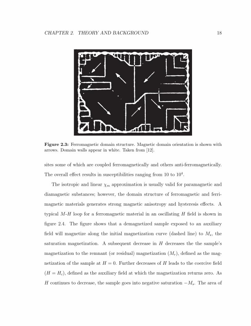
Ferro and ferrimagnetism result from a material’s chemical makeup and crystal
structure. As with paramagnetism, the atoms or molecules that comprise the crystal
have a net magnetic moment generated by unpaired valence electrons. In a ferro-
magnetic material, crystalline lattice spacings are such that valence electron spins of
adjacent atoms are aligned via the quantum mechanical exchange interaction. Aligned
moments group together in magnetic domains, as shown in figure 2.3. Domain walls
separate domains of different orientations.
External magnetic fields cause shifts in the domain structure, ultimately align-
ing magnetic domains with the field. Because domains are composed of billions of
magnetic moments, ferromagnetic materials have large magnetic susceptibilities, up
to χm ≈ 106. Ferromagnets retain some magnetization in the absence of an ~H field.
Ferrimagnetism is a combination of ferromagnetism and anti-ferromagnetism, which
is simply the opposite of ferromagnetism. Ferrite substances are composed of iron
double-oxides and at least one other metal; magnetic ions occupy different lattice
CHAPTER 2. THEORY AND BACKGROUND 18
Figure 2.3: Ferromagnetic domain structure. Magnetic domain orientation is shown witharrows. Domain walls appear in white. Taken from [12].
sites some of which are coupled ferromagnetically and others anti-ferromagnetically.
The overall effect results in susceptibilities ranging from 10 to 104.
The isotropic and linear χm approximation is usually valid for paramagnetic and
diamagnetic substances; however, the domain structure of ferromagnetic and ferri-
magnetic materials generates strong magnetic anisotropy and hysteresis effects. A
typical M -H loop for a ferromagnetic material in an oscillating H field is shown in
figure 2.4. The figure shows that a demagnetized sample exposed to an auxiliary
field will magnetize along the initial magnetization curve (dashed line) to Ms, the
saturation magnetization. A subsequent decrease in H decreases the the sample’s
magnetization to the remnant (or residual) magnetization (Mr), defined as the mag-
netization of the sample at H = 0. Further decreases of H leads to the coercive field
(H = Hc), defined as the auxiliary field at which the magnetization returns zero. As
H continues to decrease, the sample goes into negative saturation −Ms. The area of

CHAPTER 2. THEORY AND BACKGROUND 19
initial magnetization
curve
Hc
Mr
-Ms
Ms
Ma
gn
eti
zati
on
, M
Auxiliary Field, H
Hc
magnetic
Barkhausen noise
Figure 2.4: A typical magnetization hysteresis loop for a ferromagnetic sample startingwith zero magnetization. M increases with H along the initial magnetization curve tosaturation at Ms. Further variation of H changes sample magnetization as shown aroundthe loop. The inset shows magnetic Barkausen noise, which is discussed further in section2.4.1.
a B-H hysteresis loop corresponds to the energy lost to irreversible processes within
the sample [33].
2.3.1 Magnetic Domain Theory
Since the focus of the thesis is ferromagnetic materials (specifically steel), additional
discussion of their behavior is warranted, specifically with respect to their domain
configuration and behavior under magnetization. As mentioned earlier, magnetic
domains are groups of aligned magnetic moments found in ferromagnetic and ferri-
magnetic materials. Within each domain the material is magnetized to the saturation
magnetization Ms, because dipoles within each domain are aligned. Even though do-
mains are magnetically saturated, a bulk sample is generally composed of domains

CHAPTER 2. THEORY AND BACKGROUND 20
[100]
[01
0]
(a)
(b) 180o wall
90o wall
Figure 2.5: A schematic of four magnetic domains aligned along the [100] and [010]directions of Fe. (a) Each domain is made up of many aligned magnetic moments, but thefour domains together produce no net magnetization. (b) Domain walls act as transitionregions between domains of different orientation. Two types of domain wall are shown:90 and 180.
with randomly oriented magnetization vectors, producing no net sample magnetiza-
tion. An example of this is illustrated in figure 2.5(a). Figure 2.5(b) shows that
domains are separated by domain walls; these are transition regions in which mag-
netic moments gradually rotate between different orientations such that they align
with domains on either side of the wall. Domain wall thickness is a function of ma-
terial properties. In Fe, domain walls span approximately 120 atoms [7]. Domain
walls between domains with opposite magnetization vectors are termed ‘180 walls.’
Adjacent domains with perpendicular magnetizations are separated by boundaries
termed ‘90 walls.’

CHAPTER 2. THEORY AND BACKGROUND 21
The domains shown in figure 2.5 are in the [100] and [010] directions; two of the
‘easy’ crystallographic magnetization directions of the 〈100〉 set.7 Magnetic saturation
of iron in this ‘easy’ direction is achieved at a lower field density than the 〈110〉 and
〈111〉 directions, because domains with body centered cubic structures naturally align
to 〈100〉. The perpendicular arrangement of the 〈100〉 set results in strong 90 and
180 domain formation; however, the domain structure can become more complex
near surfaces and inclusions.
The magnetic domain structure of ferromagnetic materials results from the mini-
mization of the sum of six energy terms: the exchange energy (εex), the magnetocrys-
talline anisotropy energy (εmca) the magnetostatic energy (εms), the magnetoelastic
energy (ελ), the domain wall energy (εwall), and the Zeeman energy (εp). Thus, the
total energy (εtotal) for a single iron crystal is
εtotal = εex + εmca + εms + ελ + εwall + εp. (2.15)
Minimizing εtotal results in the domain structure of ferromagnetic material. Each
energy contribution is explained below.
Exchange Energy
The exchange energy (εex) is due to the quantum mechanical exchange interaction8
between adjacent atoms first described by Heisenberg in 1926 [14] and applied to
7The this document follows standard crystallographic notation. The normal of a specific plane isindicated by (100), while the set of equivalent planes is denoted by 100. Directions are indicatedby square brackets as [100]; the complete set of equivalent directions is given by angular brackets as〈100〉.
8When two atoms are adjacent, there is a finite probability their electrons will exchange places,thus the term exchange energy. Consider electron A moving about proton A and electron B movingabout proton B. As electrons are indistinguishable, there is a possibility that the electrons exchangeplaces such that electron B moves about proton A, and electron A moves about proton B. Thisconsideration introduces an additional exchange energy term into the expression for the total energyof the two atoms.

CHAPTER 2. THEORY AND BACKGROUND 22
ferromagnetism in 1928 [15]. For a set of atoms located throughout a lattice at ~ri,
each with spin ~S(~ri), the exchange energy can be written as the sum over each atom
pair [10]:
εex = −∑
jk
J (|~ri − ~rj|) ~S(~ri) · ~S(~rj), (2.16)
where J (r) is the exchange integral, which occurs in the calculation of the exchange
effect. The magnitude of J (r) drops off rapidly for large r, meaning only the nearest
neighbor spins contribute significantly to equation 2.16. If J (r) is positive, εex is a
minimum when the spins are parallel and maximum when they are anti-parallel. If
J (r) < 0, the lowest energy state results from anti-parallel spins. The alignment
of neighboring spins observed in ferromagnetism results from a positive exchange
integral.
It should be noted that the minimization of εex specifies only the orientation of
magnetic moments relative to each other, it does not specify the orientation of the
moments relative to crystallographic axes.
Magnetocrystalline Anisotropy Energy
The magnetocrystalline anisotropy energy (εmca) is the energy stored in domains
aligned to the non-easy directions of a crystal. Applied fields must do work to rotate
the magnetization direction ~Ms of a domain away from an easy direction, therefore
energy must be stored in domains aligned to non-easy directions. In 1929, Akulov
[3] showed that εmca can be expressed in terms of a series expansion of the direction

CHAPTER 2. THEORY AND BACKGROUND 23
cosines (αi, i = 1, 2, 3) of ~Ms relative to the crystal axes:9
εmca = VD
(
K0 + K1
(
α21α
22 + α2
2α23 + α2
3α21
)
+ K2
(
α21α
22α
23
)
+ ...)
, (2.17)
where VD is domain volume, and K0, K1, K2 are anisotropy constants specific to
the material (in units of J/m3). It is typical to neglect K0 in equation 2.17 because
it is independent of angle and only consider the K1 and K2 terms when evaluating
the series [6]. In Fe, εmca tends to align magnetic moments to the 〈100〉 directions,
making them directions of easy magnetization.
Magnetostatic Energy
The magnetostatic energy (εms) is the energy stored in a magnet’s demagnetizing
field, given by [6]:
εms =1
2µ0
∫
∞Hd
2 d3r, (2.18)
where ~Hd is the demagnetizing field and the integral is evaluated over all space.
In Fe, minimization of only the exchange and magnetocrystalline energies would lead
to a single magnetic domain parallel to 〈100〉; however, this configuration would
produce a significant demagnetizing field, such as that shown shown in figure 2.6(a).
The creation of an opposing domain decreases ~Hd (figure 2.6(b)), while a set of four
domains separated by 90 and 180 walls (figure 2.6(c)) further decreases ~Hd. Thus,
minimizing εms results in the formation of 90 and 180 domain walls.
9Consider a domain in a cubic crystal: let ~Ms make angles a1, a2, a3 with the crystal axes, thenα1, α2, α3 are the cosines of those angles.

CHAPTER 2. THEORY AND BACKGROUND 24
(a) (b) (c)
Figure 2.6: Demagnetizing field lines for: a) a single domain, b) two opposing domainsseparated by a 180 wall, and c) four domains separated by 90 and 180 walls.
Domain Wall Energy
Domain wall energy (εwall) is the energy associated with the formation of a single
domain wall. As shown in figure 2.5(b), a domain wall consists of a region in which
magnetic moments in adjacent atoms gradually change direction. Both εmca and
εex increase due to this gradual rotation of magnetic moments, and these increases
give εwall. The energy associated with the formation of a new wall requires that the
decrease associated with εms be greater than the corresponding increase in εwall.
Zeeman Energy
The Zeeman energy (εp) is the energy of the interaction between ~H and ~M [17], given
by
εp = −µ0
∫
∞~M · ~H d3r. (2.19)
~H is generated with free currents or permanent magnets. εp varies with ~H, leading
to changes in the magnetic energy and domain reorganization. εp is minimized when
~M and ~H are aligned.

CHAPTER 2. THEORY AND BACKGROUND 25
H
demagnetized
state
magnetic
saturation
d0
Δd
Figure 2.7: Magnetostriction of a material with positive λs.
Magnetoelastic Energy
The magnetization of a ferromagnetic material is accompanied by a change in dimen-
sion, a phenomenon termed ‘magnetostriction’ by Joule [18]. Conversely, external
stresses applied to a ferromagnetic material result in a change in magnetic properties,
a response termed the Villari effect [38]. Together, these effects are referred to as
magnetoelasticity.
Magnetostrictive strain (λ) is the strain tensor generated by magnetostriction.
The strain at magnetic saturation parallel to the direction of magnetization is termed
the saturation magnetostriction λs, shown in figure 2.7. Measurement of magne-
tostriction takes the same form as equation 2.2, giving λs = ∆d/d0. Typical λs values
are small, on the order of 10−5 and can be greater (positive magnetostriction) or less
(negative magnetostriction) than zero. Magnetostriction is anisotropic, thus different
crystalline axes have different saturation magnetostrictions, indicated by λ〈hkl〉. In
iron, λ〈100〉 = 2.1 × 10⁻⁵, while λ〈111〉 = −2.1 × 10⁻⁵.
Because of magnetostrictive anisotropy, magnetoelastic energy (ελ) is written in
terms of the saturation magnetization along specific crystalline axes; for example in

CHAPTER 2. THEORY AND BACKGROUND 26
(a) magnetostriction
HH
domain
magnetization
uniaxial
stress
auxiliary
eld
(b) Villari E"ect
σ0 σ
0
Figure 2.8: The two types of magnetoelasticity: magnetostriction and the Villari effectfor a material with positive λs. (a) A change in domain structure caused by ~H producesmagnetostrictive strains and elongation parallel to the auxiliary field. (b) Uniaxial strainresults in elongation and an increased number of 180 domains.
Fe, the 〈100〉 set is used as the reference direction, giving
ελ = −3
2λ〈100〉σ0
∫
(
cos2 γ − ν sin2 γ)
d3r, (2.20)
where σ0 is a uniaxial stress, γ is the angle between the domain magnetization and
applied stress in the sample volume, and ν is Poisson’s ratio [17]. In Fe, ελ < εmca,
meaning magnetoelastic considerations alone are insufficient to rotate the domain
orientation away from the 〈100〉 axes; however, external stress may cause preferential
alignment to a particular 〈100〉 direction.
Figure 2.8 shows the difference between magnetostriction and the Villari effect.
Increases in ~H cause expansion of domains parallel to the auxiliary field, leading to
increased sample magnetization and eventual saturation. The sample elongates as
domains grow. Conversely, the Villari effect is an increase in the number of domains
(assuming positive λs) parallel to an applied stress σ0.
CHAPTER 2. THEORY AND BACKGROUND 27
Ms
Ma
gn
eti
zati
on
, MAuxiliary Field Magnitude, H
reversibleand irreversible
wall motion
irreversible wall motion
and annihilation
domainrotation
and annihilation
H aligned to MCA direction
H misaligned withMCA directions
H misaligned withMCA directions
H aligned toMCA direction
H
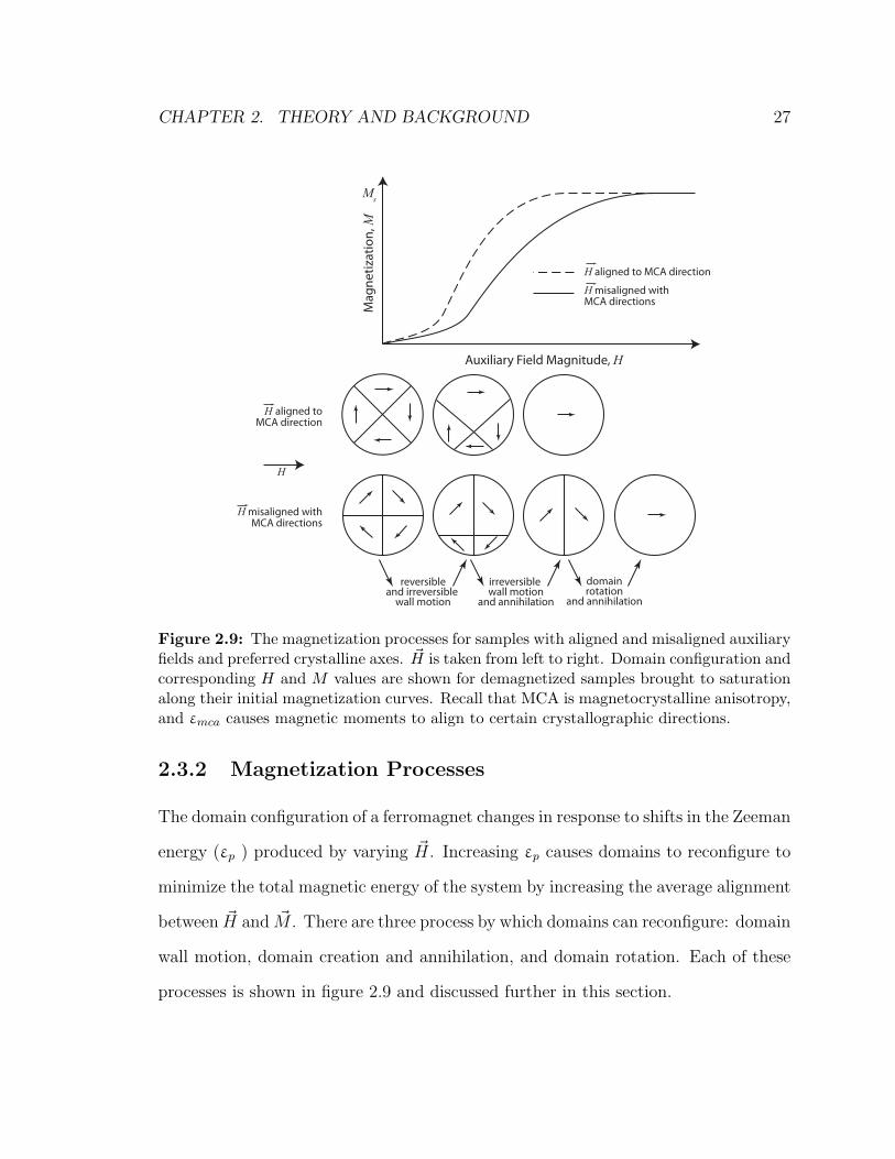
Figure 2.9: The magnetization processes for samples with aligned and misaligned auxiliaryfields and preferred crystalline axes. ~H is taken from left to right. Domain configuration andcorresponding H and M values are shown for demagnetized samples brought to saturationalong their initial magnetization curves. Recall that MCA is magnetocrystalline anisotropy,and εmca causes magnetic moments to align to certain crystallographic directions.
2.3.2 Magnetization Processes
The domain configuration of a ferromagnet changes in response to shifts in the Zeeman
energy (εp ) produced by varying ~H. Increasing εp causes domains to reconfigure to
minimize the total magnetic energy of the system by increasing the average alignment
between ~H and ~M . There are three process by which domains can reconfigure: domain
wall motion, domain creation and annihilation, and domain rotation. Each of these
processes is shown in figure 2.9 and discussed further in this section.

CHAPTER 2. THEORY AND BACKGROUND 28
Domain wall motion occurs in domains that are partially aligned to the auxiliary
field ( ~M · ~H > 0). As shown in figure 2.9, these domains increase in volume via domain
wall motion at the expense of misaligned domains. Low auxiliary fields ( ~H) produce
elastic (reversible) domain wall motion. Domain wall motion becomes irreversible at
high fields.
Misaligned domains become unfavorably small when εwall > εms. These domains
are annihilated and their moments merge with existing domains. Domain creation
and annihilation are irreversible processes. If ~H is along an axis favored by εmca,
magnetic saturation (a single domain state) will be achieved with only domain wall
motion and annihilation.
When ~H is not aligned to a favored crystalline axis, competition between εp and
εmca results in rotation of the remaining domains toward ~H, until the remaining
domains align leaving a single domain. This is shown at the bottom right of figure
2.9 where rotation results in the final saturated state.
2.3.3 Bulk Magnetic Anisotropy
Figure 2.9 shows the domain reconfiguration processes in the order (from left to right)
of the energy required to produce them. When ~H is aligned with a crystalline axis
favored by εms, domain rotation - the most energy intensive reconfiguration process
- is not required to achieve magnetic saturation; hence a single domain state can be
achieve at the lowest εp. These directions are referred to as magnetic ‘easy’ directions,
or easy axis. Bulk magnetic anisotropy occurs when an entire polycrystalline sample
displays an easy direction resulting from crystallographic texture (εmca) or strain (ελ).
Crystallographic texture (or simply ‘texture’) refers to a preferred distribution of

CHAPTER 2. THEORY AND BACKGROUND 29
crystallographic orientations in a polycrystalline sample. A random distribution of
grain orientations has no texture: no orientations are represented more than others. In
the absence of any stress influences, such a sample would be magnetically isotropic.
If a particular grain orientation is favored over others, the sample is said to have
texture in the favored orientation. Textured ferromagnetic samples tend to exhibit
bulk magnetic anisotropy, that is, they may have bulk magnetic properties that vary
with orientation. For example, the easy directions in Fe are 〈100〉, and an Fe sample
with 〈100〉 texture will have a bulk easy axis in the texture direction.
Strain can align domains to a crystallographic orientation through minimization
of ελ. Consider a tensile stress producing a tensile strain along [100] in a single Fe
crystal. ελ is minimized by increasing the population of domains aligned to [100] and
[100], forming a magnetic easy direction along [100]. In order to account for tensile
strain effects in a polycrystalline sample, a magnetic easy direction forms along the
〈100〉 directions most closely parallel to the strain. Compressive strain in Fe generates
unfavorable domain orientations, decreasing the domain population parallel to the
applied strain. Thus, compression along [100] decreases the number of [100] and [100]
domains, but increases the quantity of [010], [010], [001], and [001] domains.
2.4 Magnetic Methods of Stress Measurement
There are a number different methods of magnetic non-destructive evaluation (NDE),
all of which relate changes in a material’s magnetic properties to structural anomalies,
such as cracks, dents and pits, and localized stresses. This section reviews the theory
and use of three magnetic NDE concepts: magnetic flux leakage, magnetic Barkhausen

CHAPTER 2. THEORY AND BACKGROUND 30
noise, and stress-induced magnetic anisotropy. Magnetic flux leakage and stress-
induced magnetic anisotropy were used as the basis for sensors developed for this
thesis. Magnetic Barhkausen noise measurements were used by White for his Ph.D.
thesis, a parallel project to this thesis. The basics of magnetic Barkhausen noise NDE
are presented to enable an appreciation for the work in this thesis when compared to
White’s results.
2.4.1 Magnetic Barkhausen Noise (MBN)
Domain wall motion is not a continuous process, but rather motion that occurs in
discrete steps, as shown earlier in figure 2.4 (inset). These discontinuities are called
Barkhausen events after the physicist who discovered the effect in 1919 [4]. They occur
at frequencies up to several hundred kiloHertz, and as such can generate voltage pulses
(called Barkhausen noise) in a search coil placed nearby. The nature of Barkhausen
emissions is closely tied to the microstructure of the magnetic material and can give
insight into microscopic characteristics and stress state.
A symplified Barkhausen noise apparatus is shown in figure 2.10. An excitation
coil is driven by an AC voltage source, typically at frequencies below 1 kHz so that
the excitation field can be distinguished from the Barkhausen signal (> 100 kHz)
through bandpass or highpass filtering. Barkhausen noise signals from the sample
are detected using a pickup coil10 mounted with its axis parallel to the sample surface
normal, and can be analyzed in terms of frequency content, pulse hight distribution,
Barkhausen power density, and Barkhausen energy.
Because of the relationship between domain wall distribution and stress state,
10Also referred to as a search coil, pickup coil, or signal coil.

CHAPTER 2. THEORY AND BACKGROUND 31
core
excitation coil
sampleV
pickup coil
Figure 2.10: A simplified Barkhausen noise apparatus.
the Barkhausen spectrum can be used to evaluate stress in ferromagnetic materials.
Studies within the Applied Magnetics Group of Queen’s University frequently examine
a parameter termed ‘Barkhausen noise Energy,’ defined as
EBN =
∫ τ
0
V 2BN dt, (2.21)
where τ is the period of the excitation signal, and VBN is the voltage of the Barkhausen
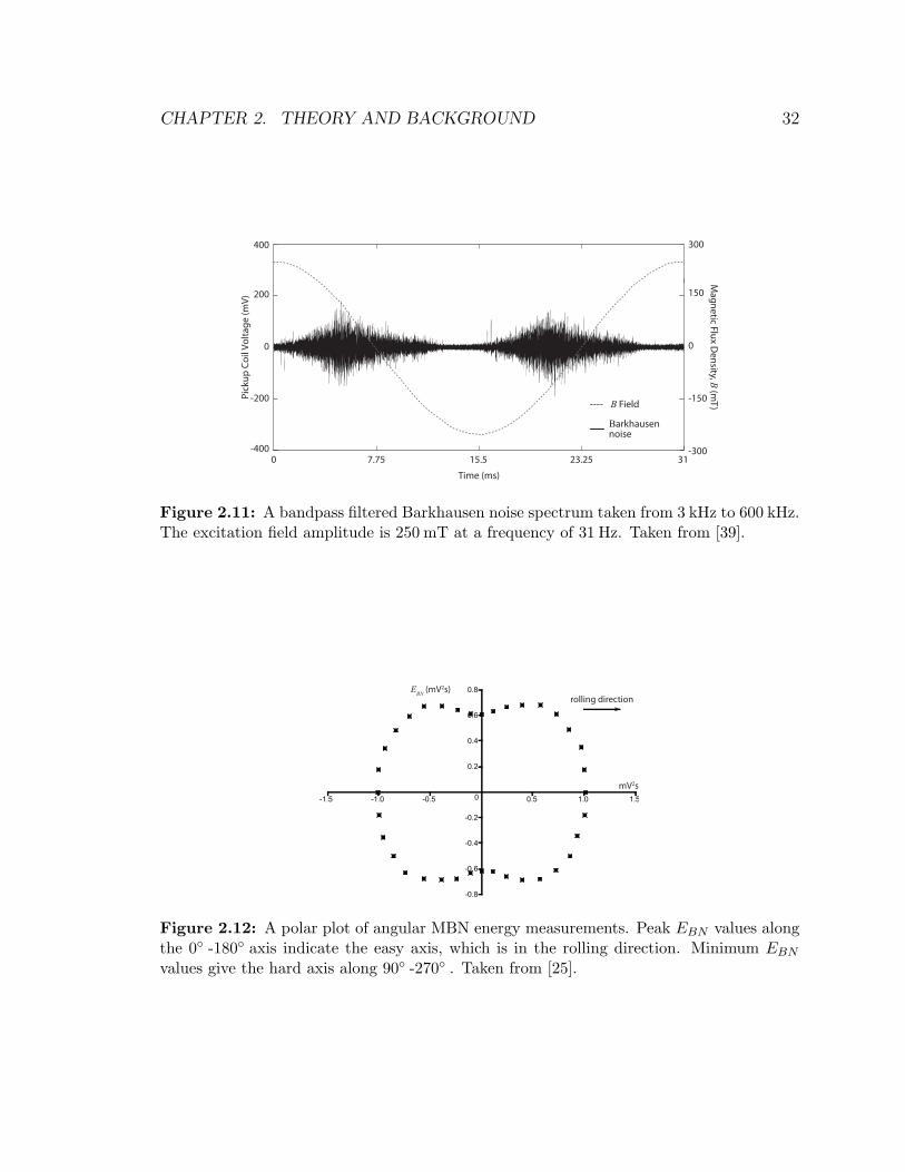
noise pulses. Figure 2.11 shows a bandpass filtered Barkhausen noise spectrum for a
sinusoidal excitation field. Barkhausen noise decreases as the sample moves toward
saturation, with peak noise occurring in the vicinity of the coercive point.
Barkhausen noise-based stress measurement methods rely on the magnetic anisotropy
introduced by stress. Barkhausen spectra such as that shown in figure 2.11 are col-
lected at regular angular intervals (typically between 5and 15 ) about a point on the
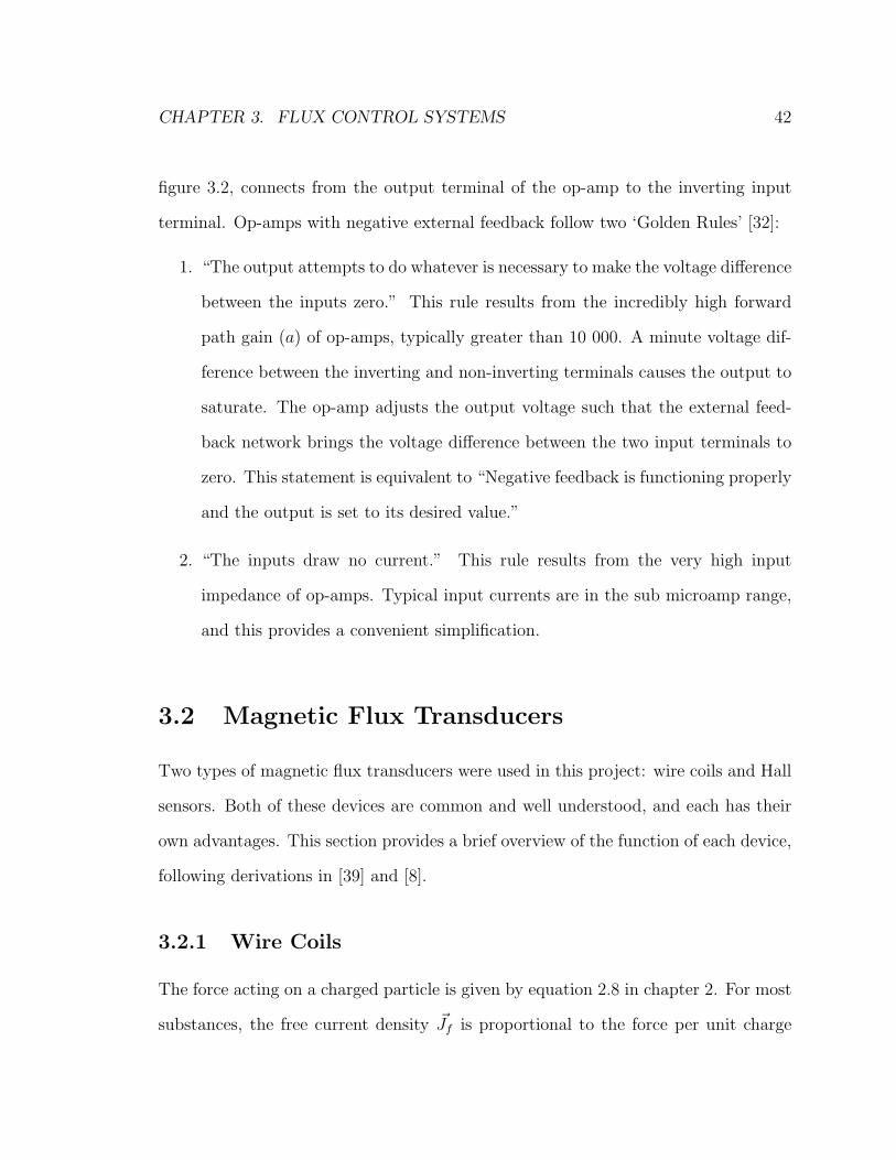
sample, and EBN is evalutated for each spectrum. Plots of EBN as a function of the
angle of the excitation field relative to a reference direction, shown in figure 2.12, give
insight into the magnetic easy direction and thus the surface stresses in the sample.
Peak Barkhausen energy occurs along the easy direction and with proper calibration
EBN can be related to stress.
Depth sensitivity is limited for Barkhausen signals due to their high frequency.
CHAPTER 2. THEORY AND BACKGROUND 32
Pic
kup
Co
il V
olt
ag
e (
mV
)
Time (ms)
Ma
gn
etic Flu
x De
nsity, B
(mT
)
0 7.75 15.5 23.25 31
0
200
400
-200
-400
300
150
0
-150
-300
B Field
Barkhausennoise
Figure 2.11: A bandpass filtered Barkhausen noise spectrum taken from 3 kHz to 600 kHz.The excitation field amplitude is 250 mT at a frequency of 31 Hz. Taken from [39].
rolling directionE
BN (mV2s)
mV2s
Figure 2.12: A polar plot of angular MBN energy measurements. Peak EBN values alongthe 0 -180 axis indicate the easy axis, which is in the rolling direction. Minimum EBN
values give the hard axis along 90 -270 . Taken from [25].

CHAPTER 2. THEORY AND BACKGROUND 33
Signal attenuation within the sample caused by eddy currents limits the maximum
depth from which Barkhausen signals can be detected to between 0.01-1.5 mm [39]
(this attenuation is discussed further in appendix B).
2.4.2 Magnetic Flux Leakage (MFL)
The magnetic flux leakage inspection method relies on the perturbation of magnetic
flux caused by defects in the sample. Localized stress may also result in MFL signals.
When examining cracks and defects, the sample is magnetized to saturation using
a strong DC field typically generated by a permanent magnet, shown in figure 2.13.
Any shifts in cross-sectional area cause magnetic flux to ‘leak’ into the surrounding
region. This ‘leakage’ flux can then be measured with an appropriate transducer,
typically a Hall probe or giant magnetoresistance sensor. Although the technique is
relatively simple in application, signal analysis is problematic, and numerous studies
within the Queen’s Applied Magnetics Group have focused on signal interpretation
for defects such as corrosion pits and generalized corrosion, dents and gouges. MFL
corrosion detection systems are widely used because of their ability to characterize the
size and depth of a flaw, and a matrix of scanners can be used to scan the complete
surface of a specimen in one pass [26].
In addition to detecting defects, the MFL technique can be utilized to probe
for regions of anomalous stress or microstructure. These regions represent localized
variations in permeability. In general these regions of permeability variation will
produce MFL signals of smaller magnitude than defect signals. Figure 2.14 shows the
MFL signal recorded by a Hall sensor scanned over the surface of SA106-B schedule
80 pipe before and after the introduction of a region of locally high stress.

CHAPTER 2. THEORY AND BACKGROUND 34
Sample
MagnetN S
Flux lines
Figure 2.13: The application of magnetic flux leakage inspection in crack and corrosiondetection.
(a)
0o
0 2.5 5 7.5 10
7.5
5
2.5
(cm)
(cm
)
0o
0 2.5 5 7.5 10
7.5
5
2.5
(cm)
(cm
)
(b)
Figure 2.14: The MFL signal from a segment of SA106-B schedule 80 pipe (a) referencemeasurement and (b) after the introduction of residual stresses through a localized impact.Maxima correspond to red and minima correspond to blue, but no further colour scaleinformation is available.

CHAPTER 2. THEORY AND BACKGROUND 35
2.4.3 Stress-Induced Magnetic Anisotropy (SMA)
In the absence of stress and texture, a polycrystalline ferromagnetic material will have
isotropic magnetic properties. The presence of stress introduces magnetic anisotropy
through minimization of ελ, an effect known as stress-induced magnetic anisotropy
(SMA). SMA measurements were pioneered by Langman in 1981 ([21], [20], [23], [22])
in a series of experiments on mild steel samples.
Langman examined the relationship between the stress state of a sample and
the angle (δ) between the magnetic field within the sample ( ~Bin) and the field just
outside the sample’s surface ( ~Bout). ~Bin was determined using two perpendicular
sensing coils wound through holes drilled in the sample. ~Bout was measured by a
Hall sensor positioned directly above the sensing coils. The Hall sensor was rotated
to determine the direction of ~Bout, while the vector sum of the sensing coil signals
provided the orientation of ~Bin. Magnetic fields were generated by an excitation
core which was rotated to provide different orientation of ~Bout and ~Bin. This section
follows the derivation of an expression for δ presented in reference [21] that will be
required for SMA signal analysis in chapter 4.
Within a uniaxially stressed sample there are typically two perpendicular principal
magnetic directions (1 and 2) of permeability µ1 and µ2, and relative permeability µr1
and µr2. In materials with positive magnetostriction (λs > 0), such as Fe, the greater
of the two permeabilities is parallel to tensile stress, while the smaller permeability is
perpendicular to it. Supposing that µ2 > µ1, then the magnetic field ~Bin within the
sample will be enhanced in the µ2 direction relative to µ1, as shown in figure 2.15.
When ~Bin is applied at an angle θ relative to µ2, the magnetic field ~Bout just outside
the sample will be rotated away from ~Bin by an angle δ.

CHAPTER 2. THEORY AND BACKGROUND 36
μ1
μ2
δ
θ
Bin1
Bin2
Bout B
in
Figure 2.15: The rotation of the magnetic field just outside the sample ( ~Bout) relative tothe magnetic field within the sample ( ~Bin) when µ2 > µ1.
δ can be determined from trigonometry using the ratio of relative permeabilities
and angle θ. Figure 2.15 shows how ~Bin can be resolved into the principle directions
as
Bin1 = B sin θ (2.22)
and Bin2 = B cos θ. (2.23)
Using ~B = µoµr
~H and assuming the sample is surrounded by air, the components of
~Bout can be resolved into the principle directions as:
Bout1 =Bin
µr1
sin θ (2.24)
and Bout2 =Bin
µr2
cos θ. (2.25)
Dividing equation 2.24 by equation 2.25 gives the ratio of external magnetic field
components as
Bout1
Bout2
=µr2
µr1
tan θ = tan(δ + θ); (2.26)
which can be rearranged to
δ = arctan
(
(µr2
µr1− 1) tan θ
1 + µr2
µr1tan2 θ
)
. (2.27)
Langman found that equation 2.27 was a reasonable prediction of the behavior of

CHAPTER 2. THEORY AND BACKGROUND 37
40
30
20
10
0
-10
-20
-30
-40
10 20 30 40 50 60 70 80
Degrees
Probe angle, φ (degrees)
Direction of Bout
relative to φ
Direction of Bin
relative to φ
Bout
Bin
Tension
μ2
φ
Figure 2.16: The orientation of ~Bin and ~Bout relative to the excitation core. The excitationcore footprint is shown by dotted lines in the inset diagram. Tensile stress was used toproduce µ2 > µ1. Taken from [21].
magnetic fields; however, it does not describe the orientation of the excitation core
relative to δ and θ. The angle between the excitation core poles and µ2, taken as φ,
is not θ or δ, but between the two. This relationship is shown in figure 2.16, which
shows that θ and δ deviate about from the probe angle (φ) by as much as 30.
Langman’s original SMA experiments were suitable for specially prepared samples
that could have perpendicular sensing coils wound through them. Later SMA mea-
surement techniques developed different sensor configurations for use on unprepared
samples, such as Kishimoto’s magnetic anisotropy sensor [34], which employs a sens-
ing coil wound around a detecting core mounted perpendicular to the excitation core

CHAPTER 2. THEORY AND BACKGROUND 38
and the sample’s surface. Modern SMA apparatus use a magnetic transducer, typi-
cally a sensing coil, oriented to measure the magnetic field perpendicular to both the
excitation field and sample surface. These coils produce no signal in isotropic sam-
ples, but SMA causes shifts ~Bout away from the excitation core so that it is detected
by the coil.

Chapter 3
Flux Control Systems
A dominant problem in magnetic NDE is ensuring that a consistent and repeatable
magnetic flux is coupled into the sample. This is a problem for all sample geometries,
including flat plates, where flux can be affected by surface preparation and varying
sample permeability. Studies on flat plates can address the issue by inserting lift-off
spacers between the magnetic field source and sample, ensuring a relatively consistent
air gap: however, the curved surfaces of pipes present a more challenging geometry.
Magnetic stress evaluation methods developed within the Queen’s Applied Mag-
netics Group rely on measuring the magnetic anisotropy in the sample [19], [37], [5].
This normally implies that sensors must be physically rotated about a location to
perform a measurement. The curvature of a pipe wall does not lend itself to sensor
rotation: air gaps change with probe orientation, thereby altering the reluctance of
the magnetic circuit for each angular measurement.
For this thesis, a new magnetic flux control system was developed to compensate
for the difficulties of magnetic flux leakage-based stress measurements on pipe ge-
ometries. This flux control system was developed in two stages: first using only Hall
39

CHAPTER 3. FLUX CONTROL SYSTEMS 40
sensor feedback (called flux control version 1 or FCV1), then expanded to both Hall
sensor and coil feedback (called flux control version 2 or FCV2).
In the following chapter, the basic principles of feedback control are presented in
section 3.1. Section 3.2 describes the magnetic transducers used for feedback control
(Hall sensors and wire coils). The components used in FCV1 and FCV2 are discussed
in section 3.3. The design, performance, and shortcomings of FCV1 are presented in
section 3.5. Section 3.6 discussed the design of FCV2 and presents a brief analysis of
its performance.
3.1 Negative Feedback Control and Operational
Amplifiers
Control systems can be separated into two groups: those without feedback (termed
open-loop), and those with feedback (termed closed-loop). Open-loop systems do not
adjust their output to changing conditions. Applied to a magnetic circuit, any distur-
bance, such as changing temperature or variable magnet liftoff, causes the output to
drift from the desired value. In a closed-loop system, shown in figure 3.1, the output
is ‘fed back’ and compared with a reference input value. The difference between the
two (called an error signal) is amplified by the forward path gain (a) to minimize
deviation between reference and output values. This type of system is said to have
negative feedback.1
There are three primary properties of negative feedback systems [35]:
1. “They tend to maintain their output despite variations in the forward path or
1There are also positive feedback systems, which sum the output and reference, but they will notbe discussed in this thesis since they were not used.

CHAPTER 3. FLUX CONTROL SYSTEMS 41
input or
referenceoutput
adder errorsignal
forward pathgain a
+
-
feedback path
Figure 3.1: The components of a closed-loop control system shown in a block diagram.The reference value is compared with the output, generating an error signal used to adjustthe output. The forward path converts inputs to outputs with the forward path gain a. Thefeedback path is the mechanism through which the output is fed back for comparison withthe reference. The error signal is the difference between the reference and output values.
in the environment.” When negative feedback is properly applied and operat-
ing stably, the output remains constant if the system is given enough time to
compensate for any changes that occur.
2. “They require a forward path gain which is greater than that which would be
necessary to achieve the required output in the absence of feedback.” Feedback
decreases overall system gain, defined as the ratio of output to input. Consider
two systems with the same forward path gain (a), one with feedback and the
other without. The system without feedback can achieve a greater overall gain
than a system with feedback.
3. “The overall behavior of the system is determined by the nature of the feedback
path.” Since feedback systems compensate for variations in the forward path,
the overall behavior of the system is determined by the feedback path.
Both FCV1 and FCV2 use operation amplifiers (op-amps), shown in figure 3.2, as
the adder and forward path mechanism, with some type of external negative feedback
mechanism to provide flux control. The feedback mechanism, which is not shown in
CHAPTER 3. FLUX CONTROL SYSTEMS 42
figure 3.2, connects from the output terminal of the op-amp to the inverting input
terminal. Op-amps with negative external feedback follow two ‘Golden Rules’ [32]:
1. “The output attempts to do whatever is necessary to make the voltage difference
between the inputs zero.” This rule results from the incredibly high forward
path gain (a) of op-amps, typically greater than 10 000. A minute voltage dif-
ference between the inverting and non-inverting terminals causes the output to
saturate. The op-amp adjusts the output voltage such that the external feed-
back network brings the voltage difference between the two input terminals to
zero. This statement is equivalent to “Negative feedback is functioning properly
and the output is set to its desired value.”
2. “The inputs draw no current.” This rule results from the very high input
impedance of op-amps. Typical input currents are in the sub microamp range,
and this provides a convenient simplification.
3.2 Magnetic Flux Transducers
Two types of magnetic flux transducers were used in this project: wire coils and Hall
sensors. Both of these devices are common and well understood, and each has their
own advantages. This section provides a brief overview of the function of each device,
following derivations in [39] and [8].
3.2.1 Wire Coils
The force acting on a charged particle is given by equation 2.8 in chapter 2. For most
substances, the free current density ~Jf is proportional to the force per unit charge

CHAPTER 3. FLUX CONTROL SYSTEMS 43
adder
errorsignal
forward pathgain a
+
-
non-invertinginput (+)
invertinginput (-)
output
V+
V-
Vo
Figure 3.2: The feedback system components contained within an op-amp. The op-ampis represented by a triangle with three terminals: the non-inverting input at voltage V+, theinverting input at voltage V−, and the output termnial at voltage Vo. The output voltageis given by the forward path gain a multiplied by the difference between the inverting andnon-inverting terminals, such that Vo = a (V+ − V−).
through conductivity σe, such that
~Jf = σe
(
~E + ~vd × ~B)
, (3.1)
where ~vd is the the average velocity of particles within the material (called the drift
velocity, because it is typically very small). Equation 3.1 is called Ohm’s law. It is
common for ~vd × ~B << ~E, thus Ohm’s law can be approximated as
~Jf = σe~E. (3.2)
Equation 3.2 is equivalent to the standard equation for resistance R in direct
current (DC) circuits:
R =V
I, (3.3)
where V is the voltage across the device, and I is the current passing through it. The
resistance is a function of conductor geometry and conductivity σe.

CHAPTER 3. FLUX CONTROL SYSTEMS 44
The electromotive force (EMF) around a closed path ∂S (E∂S)is defined as
E∂S =
∮
∂S
~E · d~l, (3.4)
and the magnetic flux through the surface S (ΦS) is defined as
ΦS =
∫
S
~B · d ~A. (3.5)
Taking ∂S to be the closed path that bounds the surface S, equation 2.5 can be
converted to integral form using Stokes’ theorem, giving∮
∂S
~E · d~l = −
∫
S
∂ ~B
∂t· d ~A. (3.6)
Equations 3.4 and 3.5 can be applied to equation 3.6 to give
E∂S = −dΦS
dt, (3.7)
where E∂S is more commonly known as the ‘back EMF.’ In the presence of a time-
varying magnetic field, electrons in a conductive material will form free currents that
oppose the existing field. These currents are generated by E∂S and are called ‘eddy
currents.’
Consider a coiled wire of resistance R carrying current I. If the coil contains N
turns of area S and is subject to a time-varying magnetic flux, the voltage across the
coil (Vcoil) is given by
Vcoil = RI + NdΦS
dt= RI + NS
dBS
dt, (3.8)
where BS is the average magnetic flux density through area S. When considering
sensing coils, the RI term in equation 3.8 is neglected, leaving only the magnetic field
term.
Equation 3.8 indicates that a voltage will be induced in a coil of wire if that coil
surrounds a region where the magnetic flux is changing. Coil wires can be used as

CHAPTER 3. FLUX CONTROL SYSTEMS 45
Jf
B
Ex
x
zy
VH
side view
top view
x
y
z
Jf
B
VH
Ex
+ + + + + + + + + + + + + + + +
- - - - - - - - - - - - - - - - - - - - - - - - -
Ey
Figure 3.3: The Hall effect for a Cartesian coordinate system. ~B is in z. Electric currentdensity ~Jf is in x, caused by the x component of ~E, Ex. Build up of electrons along the −yfacing wall produces an electric field component in the y direction, Ey. The Hall voltage(VH) is measured across the two sides facing ±y.
magnetic field sensors in air, however in many applications coils are wound around
specific components to measure the overall flux through the component. Sensing coils
are cheap and easy to manufacture. The main drawback to sensing coils is their time
dependence requirement: coils are only capable of measuring time-varying magnetic
fields. Thus they are appropriate for time-varying (AC) magnetic fields, however coils
cannot be used to measure flux in a permanent (DC) magnetic circuit. Hall sensors,
discusses in the following section, do not suffer from this limitation.
3.2.2 Hall Sensors
The Hall effect was discovered in 1879 by Edwin Hall when he attempted to determine
if the force exerted on a current carrier in a magnetic field was experienced by the
bulk of the material or only by the charge carriers (electrons) [13]. Hall discovered
a transverse voltage across the bulk of a silver test sample, perpendicular to current
flow and the magnetic field, as shown in figure 3.3. This voltage is called the Hall
voltage (VH).

CHAPTER 3. FLUX CONTROL SYSTEMS 46
Consider figure 3.3 in the absence of ~B for a metal sample: electrons flow from
right to left at drift velocity vd, generating current density Jf . With the introduction
of ~B = Bz, moving electrons are deflected in the −y direction and accumulate on
that side of the sample. Electrons continue to accumulate, increasing Ey until
Ey = vdB. (3.9)
Unfortunately, equation 3.9 is not particularly useful in this form. Drift velocities
are rarely known and it is more convenient to measure a voltage than Ey. Thus a
Hall coefficient H is used to convert equation 3.9 to
VH = HB, (3.10)
where H is a function of the probe’s charge carrier concentration, dimension, and
source current.
Sensors based on the Hall effect require a supply current. Thus Hall sensors typi-
cally have four terminals: two supply current (Ic) terminals for incoming and outgoing
supply current, and two Hall voltage terminals for the positive (VH+) and negative
(VH−) voltage values. The Hall voltage that appears in equation 3.10 measured across
the positive and negative voltage terminals as
VH = VH+ − VH−. (3.11)
Modern Hall effect sensors are semi-conducting devices that vary in cost from a
few dollars up to several hundred dollars depending on calibration qualities, response
linearity and several other parameters.
Hall sensors and wire coils measure magnetic fields by exploiting different elec-
tromagnetic effects, which lead to slightly different applications for the two sensors.
Hall sensors measure AC and DC magnetic fields, whereas coils are insensitive to

CHAPTER 3. FLUX CONTROL SYSTEMS 47
DC fields, but can be used to measure flux through specific components by winding
sensing coils around the region of interest. Hall sensors are enclosed devices and must
be placed external to any components of interest.2 The Hall voltage signal is there-
fore only proportional to the flux passing through the sensors itself. Because of this
shortcoming, the placement of Hall sensors within magnetic circuits must be made
carefully, in order that the Hall voltage signal accurately reflects the flux through the
circuit.
3.3 Component Selection
Both FCV1 and FCV2 contained similar components. The primary difference between
the systems was the feedback signal. This section outlines components common to
both FCV1 and FCV2.
3.3.1 Data Acquisition
A National Instruments R© PCI-6229 Multifunction DAQ (PCI-6229) was used to gen-
erate reference voltage signals (Vref ) and record all of the feedback system’s output
signals. This DAQ featured 4 analog output channels (AO(0...3)) with a ±10V range
about ground and 16 bit resolution. 32 single-ended multiplexed analog input chan-
nels (AI(0...31)) with a maximum sampling rate of 250 kHz aggregate over all channels
can be used for data acquisition in the PCI-6229s. Analog inputs have 16 bit resolu-
tion over each voltage range (±10V, ±5V, ±1V, ±0.2V)[28].
PCI-6229 DAQs were not purchased specifically for this project, but were used
because they were available and their specifications were adequate for both FCV1
2They cannot be placed inside a sample, and therefore cannot measure the flux inside a sample.

CHAPTER 3. FLUX CONTROL SYSTEMS 48
and FCV2.
3.3.2 Amplifier
Due to the abundance of speakers found in consumer goods, there is a large selection
of low-cost solid state power amplifiers. The excitation coils of a flux-controlled
circuit present similar load impedances to speakers found in audio equipment [39].
The National SemiconductorR© LM4701 audio amplifier3 was selected to act as the
adder/forward path in both FCV1 and FCV2 feedback systems [31]. The LM4701 is a
low noise amplifier, designed to supply 30 W into 8Ω from 20 Hz to 20 kHz with total
harmonic distortion + noise of 0.08% given proper heat dissipation. Supply voltage
can be up to ±32 V. Typical open-loop gain is a = 110 dB.
These amplifiers feature National SemiconductorR©’s SPiKeTM protection circuitry,
which protects the op-amp from voltage, current, and thermal overload.
3.3.3 Power Supply
A Power-One R© HCC24-2.4-AG regulated DC power supply with ±24 V outputs at
2.4 A was selected to provide power to amplifiers, Hall sensors, and all other compo-
nents.
3.3.4 Hall Sensors
F.W. Bell4 BH-700 Hall effect sensors were used as magnetic flux density transducers
for both FCV1 and FCV2. These sensors were used for their linear response and
3The LM4701 is now obsolete. It has been replaced by LM4765 and LM4781 multi-channelamplifiers.
4A division of Sypris Test & Measurement.

CHAPTER 3. FLUX CONTROL SYSTEMS 49
small size [9].
These Hall sensors were used in two different applications. The first, described in
this chapter, was as part of the flux control system, where the BH-700 was used to
monitor the flux density in the magnetic excitation circuit. These Hall probes were
also used as MFL stress detectors, described in chapter 4, to detect the magnetic flux
signal emanating from the sample itself. Note that in the latter case the Hall probes
are termed ‘detectors,’ in the former they are termed ‘sensors.’
3.4 White’s Flux Control System (FCS)
For his doctoral thesis dealing with magnetic Barkhausen noise, Steve White designed
a magnetic flux control system that relied on the feedback from a coil wound near the
base of an excitation core pole, termed a ‘feedback coil,’ to regulate the magnetic flux
generated by an excitation coil. This feedback system was termed the ‘Flux Control
System,’ or ‘FCS.’ Figure 3.4 is a simplified sketch illustrating the basic premise of
this control method. Vref is an arbitrary reference voltage waveform, and Vex and VF+
are voltage measurements referenced to ground. The ideal op-amp is configured as
an adder such that the sum of the currents into the inverting input through resistors
Rref , RG, and RF1 is zero
Vref
Rref
+VF+
RF 1+
Vex
RG
= 0. (3.12)
Resistors RF1 and RF2 were chosen to be much greater than the resistance of
the feedback coil. The two resistors were placed across the coil to improve system
stability. As the same current flows in RF1 and RF2, the voltage across the feedback

CHAPTER 3. FLUX CONTROL SYSTEMS 50
V F+
Vref
V ex
Rref
RF2
RG
RF1
Figure 3.4: A sketch of White’s FCS. The resistor RG was used to limit gain to providea stable output. A feedback coil wound around one of the poles acted as the flux feedbacktransducer.
coil (VF ) is given by
VF =
(
1 +RF2
RF1
)
VF+. (3.13)
Solving equations 3.12 and 3.13 for Vref gives
Vref = −
(
Rref
RF1 + RF2
)
VF −
(
Rref
RG
)
Vex. (3.14)
This system was designed to control flux independent of probe liftoff; therefore the
contribution of Vex to Vref was problematic, as Vex was unknown. Ideally, the gain-
limiting resistor RG could be removed (effectively setting RG → ∞), which would
nullify the contribution of Vex to equation 3.14. However, in this maximum-gain
configuration, any offset between the amplifier terminals would be multiplied by the
full amplifier gain (a). Without any feedback to compensate for these offsets, Vex will
gradually shift to the voltage supply rails. To avoid this issue, White maximized the
system’s performance by decreasing RG from ∞ until the circuit stabilized.
The reference voltage (Vref ) and the voltage across the feedback coil (VF ) differed
by the Vex term as
Vref = VF −
(
RF1 + RF2
RG
)
. (3.15)
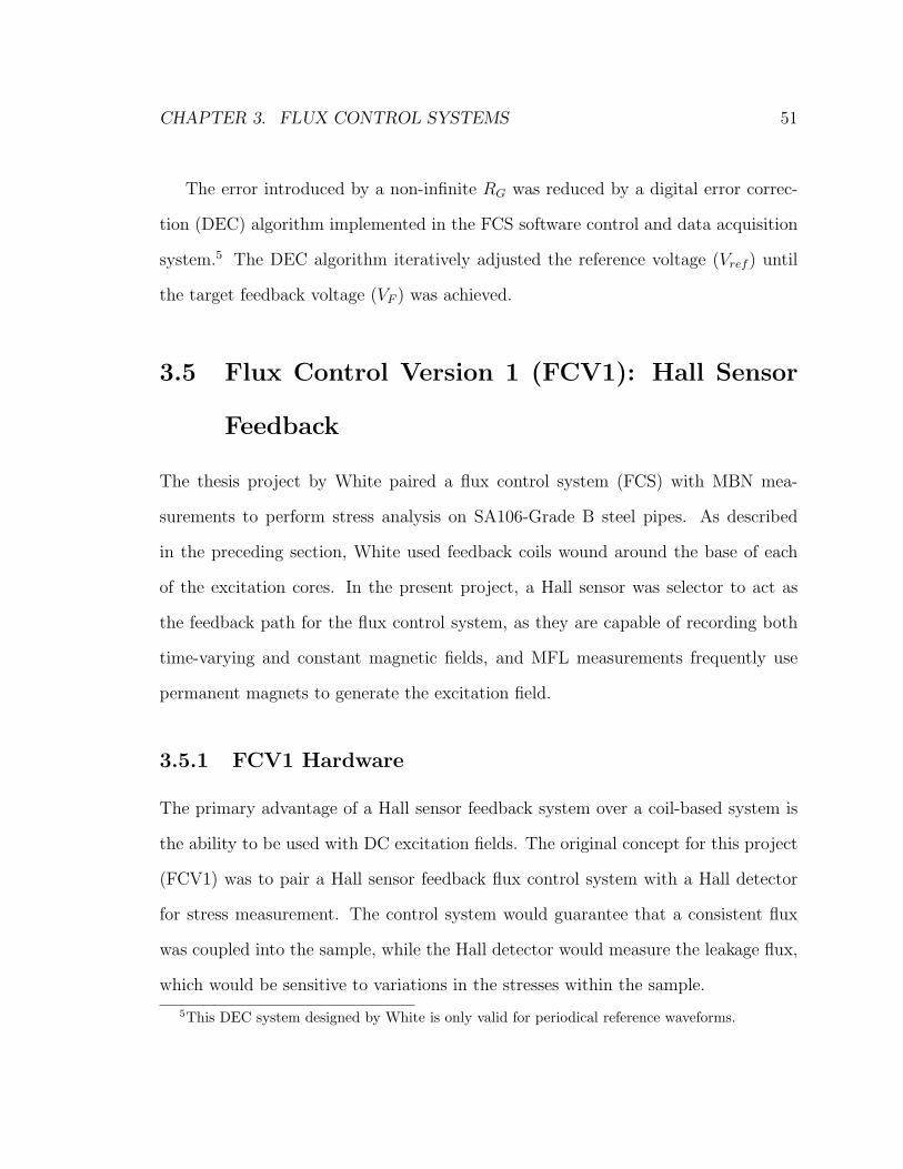
CHAPTER 3. FLUX CONTROL SYSTEMS 51
The error introduced by a non-infinite RG was reduced by a digital error correc-
tion (DEC) algorithm implemented in the FCS software control and data acquisition
system.5 The DEC algorithm iteratively adjusted the reference voltage (Vref ) until
the target feedback voltage (VF ) was achieved.
3.5 Flux Control Version 1 (FCV1): Hall Sensor
Feedback
The thesis project by White paired a flux control system (FCS) with MBN mea-
surements to perform stress analysis on SA106-Grade B steel pipes. As described
in the preceding section, White used feedback coils wound around the base of each
of the excitation cores. In the present project, a Hall sensor was selector to act as
the feedback path for the flux control system, as they are capable of recording both
time-varying and constant magnetic fields, and MFL measurements frequently use
permanent magnets to generate the excitation field.
3.5.1 FCV1 Hardware
The primary advantage of a Hall sensor feedback system over a coil-based system is
the ability to be used with DC excitation fields. The original concept for this project
(FCV1) was to pair a Hall sensor feedback flux control system with a Hall detector
for stress measurement. The control system would guarantee that a consistent flux
was coupled into the sample, while the Hall detector would measure the leakage flux,
which would be sensitive to variations in the stresses within the sample.
5This DEC system designed by White is only valid for periodical reference waveforms.

CHAPTER 3. FLUX CONTROL SYSTEMS 52
ferriteexcitationcore
excitationcoil
sample
LM4701
+
-
Ic
RsV
ref
lift-o spacer
VH+
VH-
Vmc
Vs
Vex
, IexF
GND
Hall sensor
monitoring coil
Figure 3.5: A simplified version of FCV1. A Hall sensor with supply current Ic is locatedin a plastic lift-off spacer attached to the bottom of the ferrite excitation core. This sensormeasures the B component normal to the sample surface, and feeds back a Hall voltage tobe compared to Vref .
FCV1 was designed as the Hall sensor feedback system, shown as a simplified
sketch in figure 3.5. A detailed electrical schematic of FCV1 is included in appendix
A.
Referring to figure 3.5, FCV1 was designed to control the flux entering the sample
by measuring the flux density (B) with a Hall sensor located in an air gap between
the sample and excitation core (the excitation core shown in the figure is ferrite). Vref
is the user-defined reference voltage corresponding to the desired B in the air gap.
Note that in figure 3.5, VH− is grounded, therefore VH = VH+. The voltage Vs across
a 0.2 Ω series resistor (Rs = 0.2 Ω) was monitored to measure excitation current Iex.
The output of the LM4701 was fused at 0.5 A with a slow blow fuse (F = 0.5 A) to
prevent damage to the excitation coil. A monitoring coil was wound around a pole of

CHAPTER 3. FLUX CONTROL SYSTEMS 53
excitation coilturns 1052
inductance 0.26 Hresistance 27 Ω
monitoring coilturns 37
inductance 8.7 mHresistance 1.1 Ω
ferrite excitation core pole area 264 mm2
Table 3.1: Excitation and monitor coil properties. Inductance values were recorded on-sample at 100 Hz. The monitor coil was wound around one of the core’s poles, making itsarea the same as the pole area.
Variable PCI-6229 TerminalConnection Configuration
Vref AO0 RSEVH AI0 NRSEVs AI1 NRSEVmc AI2 DIFF
GND AIsense
Table 3.2: PCI-6229 I/O assignment and terminal configuration for FCV1. Terminal con-figurations use the following abbreviations: referenced single-ended (RSE), non-referencedsingle-ended (NRSE), differential (DIFF). For additional information on terminal configu-rations see [29].
the ferrite core to monitor the FCV1 performance when operated in AC mode. The
output voltage from this coil was designated Vmc. The properties of the excitation
and monitoring coils are given in table 3.1.
Voltage input and output (I/O) was handled through the PCI-6229 board. I/O
connections and terminal configurations are given in table 3.2.

CHAPTER 3. FLUX CONTROL SYSTEMS 54
3.5.2 FCV1 LabVIEWR© Interface
FCV1 was controlled through a basic LabVIEW R© 8.5 user interface (UI), which
was developed as part of the thesis work. Vref was controlled by an included Lab-
VIEW R© waveform generator (file: ‘NI Basic Function Generator.VI’). There were
four user-specified controls: signal type, amplitude, DC offset, and frequency. The
signal type selected the output waveform as either sine, triangle, sawtooth, or square.
Amplitude, DC offset, and frequency are self explanatory. DC signals were generated
by setting the waveform amplitude to null and the DC offset to the desired value.
3.5.3 FCV1 Performance
The performance of FCV1 was examined by determining how effectively it was able
to produce an excitation field, and corresponding Hall voltage VH , that was equal to
the reference voltage waveform Vref . The Hall sensor and monitoring coil were used
to measure the excitation field. Figure 3.6 shows VH , Vref and Iex for a sinusoidal
reference voltage with an amplitude of 50 mV and a frequency of 10 Hz (Vref =
50mV sin(2πt10Hz)). Hall voltage (VH) exactly matches the reference voltage (Vref ),
making the two signals difficult to distinguish in the figure. However, VH contains a
significant noise component that is not present in Vref . This noise is also apparent in
the excitation current (Iex) waveform.
The amount of noise observed in VH and Iex was unexpected, as White’s coil-based
FCS system did not display this noise characteristic. It was found that the noise was
independent of the Vref waveform and would occur in both AC (figure 3.6)and DC
Vref (figure 3.7) system modes. Figure 3.7 indicates that noise noise in Iex peaks
at approximately 2 mA. Since the ferrite core saturates at an excitation current of
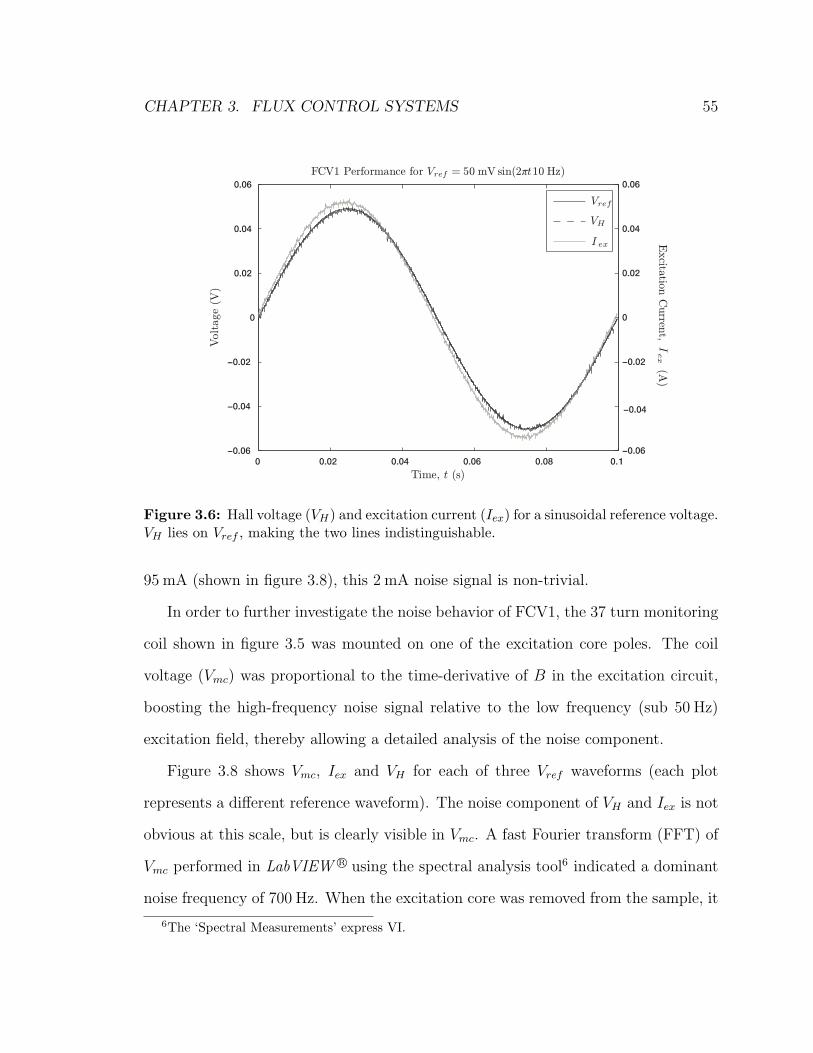
CHAPTER 3. FLUX CONTROL SYSTEMS 55
0 0.02 0.04 0.06 0.08 0.1
−0.06
−0.04
−0.02
0
0.02
0.04
0.06
FCV1 Performance for Vref = 50 mV sin(2πt10 Hz)
Time, t (s)
Volt
age
(V)
−0.06
−0.04
−0.02
0
0.02
0.04
0.06
Vref
VH
I ex
Curren
t,(A
)E
xcitation
Iex
Figure 3.6: Hall voltage (VH) and excitation current (Iex) for a sinusoidal reference voltage.VH lies on Vref , making the two lines indistinguishable.
95 mA (shown in figure 3.8), this 2 mA noise signal is non-trivial.
In order to further investigate the noise behavior of FCV1, the 37 turn monitoring
coil shown in figure 3.5 was mounted on one of the excitation core poles. The coil
voltage (Vmc) was proportional to the time-derivative of B in the excitation circuit,
boosting the high-frequency noise signal relative to the low frequency (sub 50 Hz)
excitation field, thereby allowing a detailed analysis of the noise component.
Figure 3.8 shows Vmc, Iex and VH for each of three Vref waveforms (each plot
represents a different reference waveform). The noise component of VH and Iex is not
obvious at this scale, but is clearly visible in Vmc. A fast Fourier transform (FFT) of
Vmc performed in LabVIEW R© using the spectral analysis tool6 indicated a dominant
noise frequency of 700 Hz. When the excitation core was removed from the sample, it
6The ‘Spectral Measurements’ express VI.

CHAPTER 3. FLUX CONTROL SYSTEMS 56
FCV1 Performance for Vref = 0mV
Time, t (ms)
Exci
tati
on
Curr
ent,
I ex
(mA
)
0 20 40 60 10080
3
2
1
0
-1
-2
-3
Figure 3.7: FCV1 response to a DC reference voltage of Vref = 0. Only the excitationcurrent waveform is shown. VH was omitted for clarity.
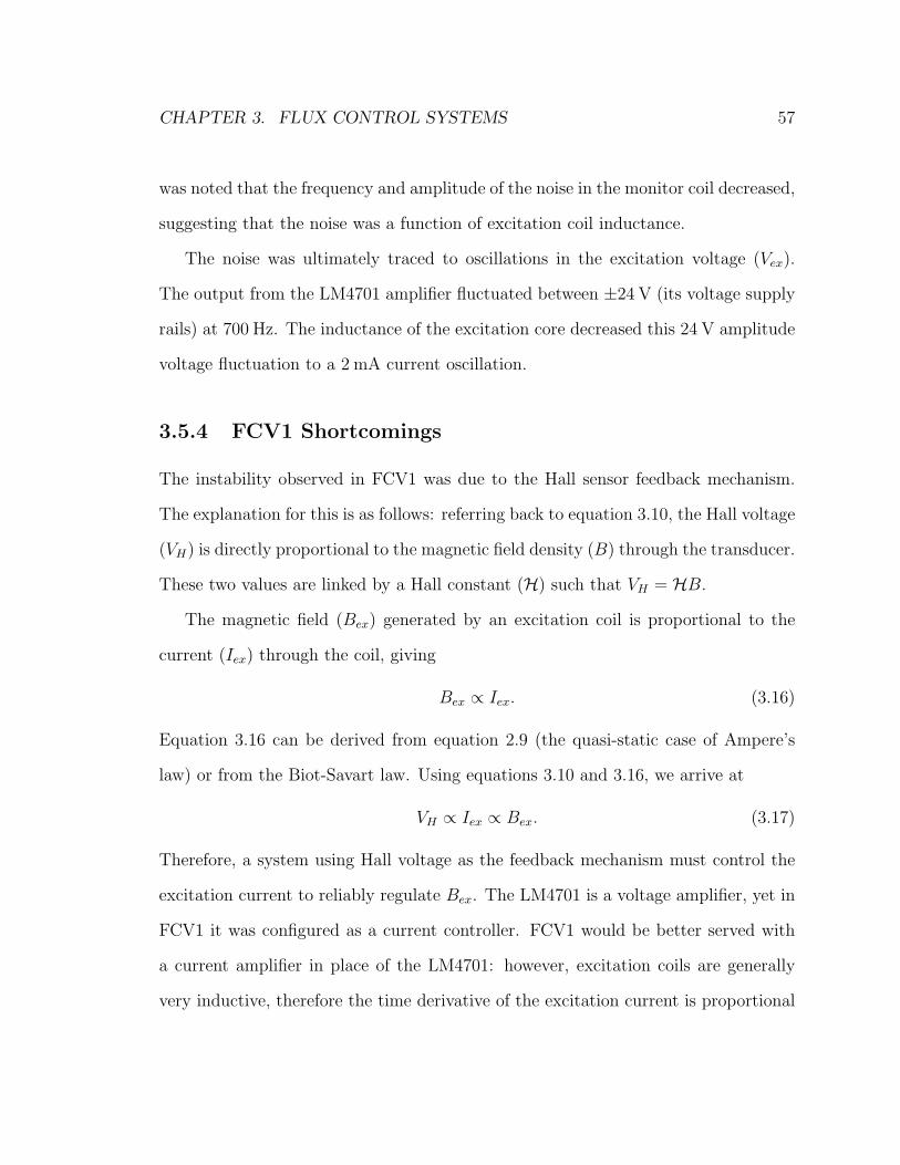
CHAPTER 3. FLUX CONTROL SYSTEMS 57
was noted that the frequency and amplitude of the noise in the monitor coil decreased,
suggesting that the noise was a function of excitation coil inductance.
The noise was ultimately traced to oscillations in the excitation voltage (Vex).
The output from the LM4701 amplifier fluctuated between ±24 V (its voltage supply
rails) at 700 Hz. The inductance of the excitation core decreased this 24 V amplitude
voltage fluctuation to a 2 mA current oscillation.
3.5.4 FCV1 Shortcomings
The instability observed in FCV1 was due to the Hall sensor feedback mechanism.
The explanation for this is as follows: referring back to equation 3.10, the Hall voltage
(VH) is directly proportional to the magnetic field density (B) through the transducer.
These two values are linked by a Hall constant (H) such that VH = HB.
The magnetic field (Bex) generated by an excitation coil is proportional to the
current (Iex) through the coil, giving
Bex ∝ Iex. (3.16)
Equation 3.16 can be derived from equation 2.9 (the quasi-static case of Ampere’s
law) or from the Biot-Savart law. Using equations 3.10 and 3.16, we arrive at
VH ∝ Iex ∝ Bex. (3.17)
Therefore, a system using Hall voltage as the feedback mechanism must control the
excitation current to reliably regulate Bex. The LM4701 is a voltage amplifier, yet in
FCV1 it was configured as a current controller. FCV1 would be better served with
a current amplifier in place of the LM4701: however, excitation coils are generally
very inductive, therefore the time derivative of the excitation current is proportional

CHAPTER 3. FLUX CONTROL SYSTEMS 58
0 0.02 0.04 0.06 0.08 0.1- 0. 2
- 0. 1
0
0.1
0.2
0.3
Time, t (s)
0 0.02 0.04 0.06 0.08 0.1- 0. 4
- 0. 2
0
0.2
0.4
Time, t (s)
Volt
age
(V)
Vref = 95 mV sin(2πt20 Hz)
0 0.02 0.04 0.06 0.08 0.1- 0. 4
- 0. 2
0
0.2
0.4
Time, t (s)
Volt
age
(V)
Vref = 50 mV sin(2πt30 Hz)
Vref = 95 mV sin(2πt10 Hz)Volt
age
(V)
0.1
0.05
0
- 0.05
- 0.1
0.2
0.1
0
- 0.1
- 0.2
0.2
0.1
0
- 0.1
- 0.2
0.3
Curren
t,(A
)E
xcitation
Iex
Curren
t,(A
)E
xcitation
Iex
Curren
t,(A
)E
xcitation
Iex
Vmc
VH
I ex
(a)
(b)
(c)
Figure 3.8: Monitor coil voltage Vmc boosts the noise amplitude relative to the excitationfield. Waveforms for three different sinusoidal reference voltages are shown: two 95 mVsignals at 10 and 20 Hz (figures (a) and (b)), and a 50 mV signal at 30 Hz (figure (c)).A 95 mV reference voltage amplitude was enough to drive the ferrite core to saturation,indicated by the lumps at peak Iex values.

CHAPTER 3. FLUX CONTROL SYSTEMS 59
to the excitation voltage (Vex) such that
dIex
dt∝ Vex. (3.18)
Equation 3.18 indicates that to effectively control current through an excitation coil,
the current amplifier requires infinite voltage rails. These systems simply do not exist.
White’s FCS system relied on LM4701 amplifiers paired with coils as the feedback
mechanism. The voltage across a feedback coil (Vfc) wound around the pole of the
excitation core is then proportional to time-derivative of the flux through the core,
giving
Vfc ∝dBex
dt. (3.19)
The proportionality arguments of equations 3.16, 3.18 and 3.19 lead to
Vfc ∝dBex
dt∝ Vex. (3.20)
This direct proportionality between the feedback coil signal Vfc and excitation coil
voltage Vex indicates that a coil-based feedback mechanism is better suited for voltage
control of a standard operational amplifier. This was the premise of the second flux
control system, FCV2.
It should be noted that further investigation and analysis of the dynamic proper-
ties of FCV1 may have resolved the instability observed in the system. However, due
to time constraints and the fact that the FCS system functioned properly, FCV1 was
abandoned in favor of a new design with coil feedback.

CHAPTER 3. FLUX CONTROL SYSTEMS 60
3.6 Flux Control Version 2 (FCV2): Hall Sensor
and Coil Feedback in Combination
While Hall sensors are well suited to current controlled flux control systems systems,
voltage controlled systems are best coupled with feedback coils. In Steven White’s
thesis work, the flux control system used feedback coils paired with LM4701 ampli-
fiers to regulate the flux passing through samples. This is why the FCS excitation
signals contained significantly less noise than those produced by the FCV1 system in
the current study. However, relying on coil feedback only requires error correction
software to compensate for DC offsets in the system.7 The second design employed in
the current project, FCV2, was designed with both coil and Hall sensor feedback to
eliminate the need for error correction software and to provide a fully hardware-based
magnetic flux controller.
3.6.1 FCV2 Hardware
A new amplifier configuration was required to combine Hall sensor and feedback coil
control. As with the FCV1 system, an LM4701 op-amp was used to power the FCV2
circuit, which is shown in figure 3.9. B was measured through the ferrite excitation
core by integrating the monitor coil into the feedback loop, producing Vfc, and also (as
with FCV1) in the air gap between the core and sample by a Hall sensor, producing
VH+ and VH−. Note that both of the Hall voltage terminals were allowed to float in
FCV2.
FCV2 can be analyzed according to the Golden Rules given in section 3.1. When
7See [39] p. 73.

CHAPTER 3. FLUX CONTROL SYSTEMS 61
ferriteexcitationcore
excitationcoil
sample
LM4701
+
-
Ic
Rs
Vref
lift-o spacer
VH+
VH-
Vfc
Vs
Vex
, IexF
GND
VH+
VH-
Vfc
Rref
RH
RH
Rfc
RG
RG
V+
V-
Hall sensor
feedbackcoil
Figure 3.9: A simplified version of FCV2. There are only a few changes from figure 3.5.Vfc has been integrated into the feedback circuit, and one end of the feedback coil wasgrounded. Neither VH+ or VH− was grounded.

CHAPTER 3. FLUX CONTROL SYSTEMS 62
the inverting (-) and non-inverting (+) terminals to draw no current, the voltages at
each terminal, V− and V+ respectively, are given by
V+ =RG(VrefRH + VH−Rref )
RHRG + RrefRG + RrefRH
(3.21)
and
V− =RG(VfcRH + VH+Rfc)
RHRG + RfcRG + RfcRH
. (3.22)
Negative feedback was used, therefore the voltage at both input terminals must be
the same, giving
V+ = V−. (3.23)
When RG = RH = Rfc = Rref , equations 3.21, 3.22, and 3.23 can be solved for Vref
to give
Vref = Vfc + VH+ − VH− = Vfc + VH . (3.24)
Equation 3.24 can be written in terms of the excitation field Bex(t), feedback coil
turns (Nfc), feedback coil area (Afc) and Hall constant H, such that
Vref (t) = NfcAfcdBex(t)
dt+ HBex(t). (3.25)
Figure 3.9 is a simplified version of FCV2, useful for a general discussion of the
feedback system and reference voltage waveform. Figure 3.10 presents a more detailed
electrical schematic of the feedback system including the current source used for BH-
700 Hall sensors in FCV2. The Hall sensor control current (Ic) was supplied by
a National Semiconductor LM337 negative voltage regulator run in current-control
mode [30]. The 0.2 and 180 Ω resistors in series with the BH-700 sensor put VH+ and
VH− within the PCI-6229’s ±10 V input range.8 Resistors in the feedback system
8VH was always less than 1 V, but VH+ and VH− had to be within ±10 V of ground for thePCI-6229 to make the differential measurement VH = VH+ − VH−.

CHAPTER 3. FLUX CONTROL SYSTEMS 63
In
Out
Adj
LM337
BH-700
+Ic
-Ic
VH+
VH-
Red
Blue
Yellow
Black-
LM4701
+
1 μF
-24 V
1 μF
+24 V
Vref
VH+
VH-
1 kΩ
1 kΩ
1 kΩ
1 kΩ
1 kΩ
-24V
10 Ω1μF
1 kΩV
fc
1
23
1
2
3,54
8
7
180 Ω
0.2 Ω
Ic
10 kΩ 1 kΩ
10 MΩ
VsF = 0.5A R
ex Lex
Rfc
Lfc
Vex
111
0.2 Ω
excitation coil
feedback coil
feedback Hall sensor current supply
Figure 3.10: An electrical schematic of FCV2 showing the feedback system and the Hallsensor current source. The LM4701 acts as an amplifier and adder for the feedback system.The Hall sensor current source is the LM337 voltage regulator, configured in current-controlmode. Pin numbers are shown for the LM4701 and LM337, as well as BH-700 lead colors.White circles indicate external connections to voltage supplies (±24 V) or to the PCI-6229DAQ (Vref , VH−, VH+, Vfc, Vs, Vex).
were set to 1kΩ, while the fuse and series resistance (Rs) were unchanged from FCV1
(F = 0.5 A and Rs = 0.2 Ω).
A voltage divider of 10 kΩ and 1 kΩ resistors, giving a voltage divider ratio of
1/11, was used to directly measure the excitation voltage; a parameter that had not
been examined in FCV1. The divider was required to bring the maximum excitation
voltage |Vex| = 24 V into the measurement range of the PCI-6229 DAQ.
The PCI-6229 terminals were reconfigured to accommodate the new feedback
system. I/O connections and terminals configurations for FCV2 are given in table

CHAPTER 3. FLUX CONTROL SYSTEMS 64
Variable PCI-6229 TerminalConnection Configuration
Vref AO0 RSEVH AI0 DIFFVs AI1 NRSEVfc AI2 DIFFVex AI3 NRSEVsig AI4 DIFF
GND AIsense
Table 3.3: PCI-6229 I/O assignment and terminal configuration for FCV2.
3.3. A sensor input line that recorded the magnetic detector output signal (Vsig) was
added as a differential input.
3.6.2 FCV2 Software
The software and user interface was rebuilt for FCV2. LabVIEW R© Express VIs used
for data acquisition and signal generation in FCV1 were replaced with purpose-built
timing and triggering code. This improved synchronization between input and output
channels, and improved the voltage and time resolution of the data acquisition system.
Excitation and feedback coil parameters, such as those in table 3.1, were used to
calculate Vfc, VH , and subsequently Vref for a user-specified excitation magnetic field
density (Bex). The transition from the user-specified reference voltage used in FCV1
to Bex for FCV2 was done to highlight the relationship between Vfc, VH , and Bex
shown in equation 3.25.
Degaussing code was added so that any residual magnetization resulting from
previous measurements or magnetic exposure could be removed from the sample prior
to measurements. This ensured that measurements with FCV2 could be performed
on demagnetized samples. This code was absent in FCV1 because the system never
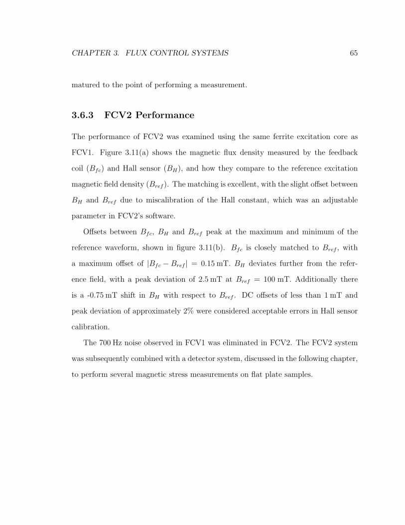
CHAPTER 3. FLUX CONTROL SYSTEMS 65
matured to the point of performing a measurement.
3.6.3 FCV2 Performance
The performance of FCV2 was examined using the same ferrite excitation core as
FCV1. Figure 3.11(a) shows the magnetic flux density measured by the feedback
coil (Bfc) and Hall sensor (BH), and how they compare to the reference excitation
magnetic field density (Bref ). The matching is excellent, with the slight offset between
BH and Bref due to miscalibration of the Hall constant, which was an adjustable
parameter in FCV2’s software.
Offsets between Bfc, BH and Bref peak at the maximum and minimum of the
reference waveform, shown in figure 3.11(b). Bfc is closely matched to Bref , with
a maximum offset of |Bfc − Bref | = 0.15 mT. BH deviates further from the refer-
ence field, with a peak deviation of 2.5 mT at Bref = 100 mT. Additionally there
is a -0.75 mT shift in BH with respect to Bref . DC offsets of less than 1 mT and
peak deviation of approximately 2% were considered acceptable errors in Hall sensor
calibration.
The 700 Hz noise observed in FCV1 was eliminated in FCV2. The FCV2 system
was subsequently combined with a detector system, discussed in the following chapter,
to perform several magnetic stress measurements on flat plate samples.

CHAPTER 3. FLUX CONTROL SYSTEMS 66
0 5 10 15 20−100
−80
−60
−40
−20
0
20
40
60
80
100
Time, t (ms)
Magnet
icFie
ldD
ensi
ty(m
T)
FCV2 Performance for Bref = 100 mT sin(2πt55 Hz)
BrefBHBfc
0 5 10 15 20
Time, t (ms)
Magnet
icFie
ldD
ensi
ty(m
T)
Hall Sensor and Feedback Coil Magnetic Field
BHBfc
BrefBref
--
1.5
1
0.5
0
-0.5
-1
-1.5
-2
-2.5
-3
(a)
(b) Offsets
Figure 3.11: The magnetic fields measured by the Hall sensor and feedback coil in FCV2.(a) The reference field was 100 mT in amplitude at a frequency of 55 Hz. Bref and Bfc
curves lie on top of each other, making them nearly indistinguishable. Offsets, shown in thebottom figure (b), were calculated by subtracting measured field density (Bfc, BH) fromBref .

Chapter 4
Magnetic Stress Detectors
The magnetic excitation system based on FCV2 provided an effective, consistent and
repeatable method of coupling magnetic flux into samples. The next stage in the
process involved adding a detector to measure the magnetic signal emanating from
the sample when an excitation field was generated by FCV2.
A this point it is convenient to define some important terms. The ‘detector’ refers
to the magnetic flux transducer used to measure stress-induced leakage flux emanating
from the sample. This detector is located between the poles of the excitation magnet
and can be either a wire coil or a Hall probe. Detectors are not to be confused with
feedback ‘sensors’ (referring to the feedback Hall sensor and feedback coil sensor) used
in the excitation flux control system. Finally, the term ‘probe’ refers to the entire
physical device, consisting of the detector, excitation coil, core, feedback Hall sensor
and feedback coil.
Three detector configurations were tested with the FCV2 probe. These configu-
rations are shown in figure 4.1. The first, figure 4.1 (a), was a Hall detector aligned
parallel to the sample surface normal, termed the ‘DC MFL’ detector. The second,
67

CHAPTER 4. MAGNETIC STRESS DETECTORS 68
(b)(a)
(c)
wire coil
Hall detector
measured B component
Figure 4.1: The three detector configurations used with the prototype excitation core.(a) DC MFL: a Hall detector oriented parallel to the surface normal. (b) AC MFL: a wirecoil with its axis parallel to the surface normal. (c) SMA: a wire coil with the coil axisperpendicular to a line between the excitation core poles and the surface normal.
shown in figure 4.1 (b), was a wire coil with its axis aligned to the sample surface
normal, termed the ‘AC MFL’ detector. Finally, figure 4.1 (c) shows a wire coil with
its axis perpendicular to both the sample surface and a line joining the poles of the
excitation core. This was termed the ‘SMA’ detector and was used for stress-induced
anisotropy measurements.
A flat plate sample subjected to a variable uniaxial applied load was used to evalu-
ate the stress sensitivity of the probe for each of the the three detector configurations.
The remainder of this chapter is organized in the following sections:
• Section 4.1 provides an overview of the steel sample and the Single Axis Stress
Rig - the apparatus used to apply stress to the sample.
• Section 4.2 describes in detail the three detector configurations shown in figure
4.1, as well as the data acquisition system.
• Section 4.3 outlines the experimental procedures used to test the three detector

CHAPTER 4. MAGNETIC STRESS DETECTORS 69
configurations
• Section 4.4 presents the results for each of the detector tests.
4.1 Test Sample and the Single Axis Stress Rig
(SASR)
To determine the effectiveness of different detector configurations, a flat plate sample
was subjected to a uniaxial tensile stress via a single axis stress rig (SASR). Details
of the test sample and SASR are described here.
4.1.1 Test Sample
Measurements were performed on a 2.8 mm thick hot-rolled mild steel plate, 500 mm
long and 216 mm wide, shown in figure 4.2. Tensile strength tests on these samples
indicated a yield strength of 291 MPa, a Young’s modulus of Y = 219 GPa [2], and
Poisson’s ratio to be ν = 0.278 [24].
The sample was used in previous Ph.D. thesis work by Catalin Mandache [24].
For this work, two electrochemically milled 18 mm diameter holes were located in the
center of the plate. A total of three Vishay R© Measurements Group EA-06-250BF300
strain gages were mounted at different locations on the plate, as indicated in figure 4.2.
Strain gage 1 measured the strain along the length of the plate, which corresponded
to the applied stress direction. Gages 2 and 3, located on the opposite side of gage
1, were used to determine the uniformity of the applied strain.
Measurements using the prototype probes were performed at the location indi-
cated in figure 4.2. This location was selected to avoid any stress concentrations or

CHAPTER 4. MAGNETIC STRESS DETECTORS 70
500
216
125
108
94.5
271
8
applied tensile stress σt
in the ‘parallel’ direction
in t
he ‘
perp
en
dic
ula
r’ d
irecti
on
measurement
location
strain
gage 1
strain
gage 2
strain
gage 3
co
mp
ressiv
e s
tress σ
c =
-νσ
t
Figure 4.2: The mild steel plate used to test different detector configurations. Strain gagelocations are shown by rectangles. Gage 1, indicated by a dashed line, was located on theunderside of the plate. Gages 2 and 3 were located on the upper plate surface. Two 18 mmhole defects were at the center of the plate. All dimensions are in mm.
other localized stress effects resulting from the sample edges or hole defects.
4.1.2 The Single Axis Stress Rig (SASR)
The single axis stress rig (SASR) was designed and built within the Applied Magnetics
Group to serve as a general purpose stressing device for the application of tensile
stresses. It was configured to apply to ‘single axis’ tensile loads along the length of
flat plate samples, such as that indicated in figure 4.2.
A schematic diagram of the SASR is shown in figure 4.3. Two sets of steel jaws
clamp down on either end of the sample. One set of jaws is connected to a fixed
bridge, while the other is connected to a gliding bridge that moves along guidance
rods. Two hydraulic jacks extend when pressurized by a manual pump. Extension
of the pistons within the hydraulic jacks pushes the gliding bridge along the guide
rods, applying tensile stress (σt) to the sample clamped in the jaws. As a result of

CHAPTER 4. MAGNETIC STRESS DETECTORS 71
xed bridge
sample jaws
sample
gliding bridge
guidance rods
spacer cylinder
hydraulic jack
support beam
Figure 4.3: A schematic of the single axis stress rig used to introduce tensile stress in theflat plate sample.
Poisson’s ratio effects, compressive stress is also generated across the width of the
sample (σc) given by
σc = −νσt. (4.1)
The pressure in hydraulic lines was monitored by an Omega Engineering Inc.
PX302-10KGV pressure transducer connected to an Omega Engineering Inc. DP25-S
digital meter. A more detailed description of the SASR and its operation is provided
in reference [24].
4.1.3 Strain Measurement
The three EA-06-250BF300 strain gages mounted on the sample were connected to
a Vishay R© Measurements Group SB-10 Balance and Switch used to calibrate the
strain gages and sequentially switch between the output of each gage. The SB-10 was
connected to a Vishay R© Measurements Group P3500 Strain Indicator, which provided
a direct indication of the strain measured by the gages.

CHAPTER 4. MAGNETIC STRESS DETECTORS 72
64 mm
R 9.2 mm
feedback coil
ferrite excitation core
excitation coil
detector mount assembly
outer brace
connector brace
feedback Hall sensor
housed within a lifto! spacer
lifto! spacer
detector mount assembly
detector brace
(a) (b)
Figure 4.4: An assembled probe showing a detector mount assembly attached to theconnector brace of the excitation core. (a) Important components are indicated in thefigure. The spring of the detector mount is not visible in this figure; it is hidden betweenthe detector brace and outer brace. (b) A photo of the assembled system, built by theauthor.
4.2 Detectors, Data Acquisition and Data Analy-
sis
The three different detectors - DC MFL, AC MFL, and SMA - were attached to the
excitation core with a detector mount assembly, shown in figure 4.4(a). The detector
mount assembly consisted of three primary parts: a detector brace that housed the
detector, a spring (not shown) to push the detector brace against the sample, and
an outer brace that housed the detector and spring system and attached it to the
excitation core. Each of the detectors was fixed to its own mounting assembly, which
could be quickly connected to the excitation core. The assembled core and detector
system is called a probe. A photograph of the assembled probe is shown in figure
4.4(b)

CHAPTER 4. MAGNETIC STRESS DETECTORS 73
Figure 4.5 shows a plan, underside view of each detector mounted to the excitation
core. The details of each detector are outlined below.
DC MFL
The Hall sensor used for DC MFL measurements was a F.W. Bell BH-700 sensor;
this was the same Hall sensor used in both FCV1 and FCV2 flux control systems.
The processed1 output signal from this detector was denoted VDCM .
AC MFL
An air-core 200 turn coil wound from 44 AWG wire with an average loop area of
3.1 mm2 was used for the AC MFL detector. This coil was circular with an inner
diameter of 0.98 mm and an outer diameter of 2.99 mm. The processed output voltage
of this detector was denoted VACM .
SMA
The SMA detector was a rectangular air-core 69 turn coil wound from 44 AWG wire
with an area of 2.86mm2. The coil was 2.15 mm long and 1.35 mm high. The 2.15 mm
length dimension lay along the sample’s surface, while the height dimension projected
away from it. The coil was constructed as a rectangle, and oriented as described, in
order to maximize the ‘measurement region’ in close proximity to the sample’s surface.
VSMA denoted voltage of this detector after signal processing.
1The output voltage signals of the detectors were acquired as Vsig by the LabVIEW R© software:however, each detector required different signal processing methods, such as averaging and fitting,to produce a useful signal. The signal processing for each detector is outlined in section 4.4.

CHAPTER 4. MAGNETIC STRESS DETECTORS 74
AC MFLDC MFL SMA
Figure 4.5: DC MFL, AC MFL, and SMA detectors mounted to the excitation core. Thedetectors were locked into their mounts with epoxy. The detectors are not shown to scale.
4.2.1 Data Acquisition
Signals from the three different detectors were acquired by the PCI-6229 DAQ as Vsig,
configured as indicated in table 3.3 (located in chapter 3).
The DC MFL, AC MFL, and SMA detector signals were conditioned differently
depending on the output voltage magnitude of each transducer. DC MFL measure-
ments were input directly to the PCI-6229 as a differential measurement across the
VH+ and VH− terminals of the Hall detector. AC MFL and SMA signals were ampli-
fied by an Ithaco R© Model 565 preamplifier in transformer mode, producing a gain of
60 dB prior to being input into the PCI-6229.

CHAPTER 4. MAGNETIC STRESS DETECTORS 75
AC MFL and DC MFL
tensile measurement
Bex
AC MFL and DC MFL
compressive measurement
Bex
Bex
SMA measurement
0o
90o
180o
270o
applied tensile
stress σt σ
tσt
com
pre
ssiv
e s
tre
ss σ
c
σc
σc
Figure 4.6: The footprint of the excitation core on the sample for AC MFL, DC MFL andSMA measurements. The direction of ~Bex is indicated by white lines between the excitationcore poles.
4.3 Experimental Procedures for Testing and Com-
parison of the Probe Systems
Tensile stress was applied to the sample by pressurizing the hydraulic jacks of the
SASR. Measurements were performed with each of the three detector/probe combina-
tions: DC MFL, AC MFL, and SMA. These measurements were recorded at different
stress levels to determine which detector was most sensitive to stress effects.
Figure 4.6 shows the orientation of the probe excitation core relative to the stress
direction for DC MFL, AC MFL and SMA detectors. As shown in the first two dia-
grams of figure 4.6, AC MFL and DC MFL measurements were performed with the
probe parallel (called the ‘parallel’ configuration) and perpendicular (called the ‘per-
pendicular’ configuration) to the applied stress. The parallel configuration enabled a
measurement of tensile strain sensitivity, while the perpendicular configuration was
a measurement of compressive strain2.
SMA measurements were performed by rotating the probe over 360 about the
2The SASR could only produce tensile strain. The Poisson effect was exploited to examine ACMFL and DC MFL compressive sensitivity.

CHAPTER 4. MAGNETIC STRESS DETECTORS 76
measurement location, stopping to make measurements at 15 intervals. Thus, each
‘stress measurement’ consisted of 25 data sets3. Taking φ as the angle between the
probe and the direction of tensile stress, φ = 0, 180, 360 probe orientations aligned
the probe along σt, the applied stress direction, while φ = 90, 270 aligned the
probe with the largest compressive stress (σc) direction. φ was taken to increase
anti-clockwise from zero.
All measurements were performed within the elastic deformation range of the
sample. A degaussing cycle4 was completed before each measurement to remove any
residual magnetization from the sample.
4.4 Detector Results and Analysis
Voltage signals from the DC MFL, AC MFL, and SMA detectors were recorded in
the FCV2 software as signal voltage (Vsig) waveforms. This section describes the
method by which raw Vsig waveforms were processed to produce VDCM , VACM and
VSMA values. Each detector/probe system is considered in this section.
4.4.1 DC MFL
DC MFL measurements were performed using the probe with an excitation field mag-
nitude of 100 mT on flat plate samples in the SASR. A DC MFL Hall detector voltage
(VDCM) measurement was recorded for increasing stress values up to a maximum ten-
sile stress of 107 MPa.
3There were a total of 25 waveforms recorded for each SMA measurement because data wasacquired at both φ = 0 and φ = 360.
4A degauss cycle removes residual magnetization from the sample by cycling through hysteresisloops of decreasing magnitude.

CHAPTER 4. MAGNETIC STRESS DETECTORS 77
The configuration of the FCV2 software interface required that the DC excita-
tion fields used in DC MFL measurements were input as sine functions with null
amplitude, a 15 Hz frequency, and a 100 mT offset term. This resulted in ‘DC MFL
Vsig distributions’ consisting of 3333 Vsig data points recorded over a 67 ms window.
3333 data points for a 15 Hz signal corresponds to the system’s sampling frequency
of 50 KHz, while 67 ms is simply the period of a 15 Hz wave.
VDCM was taken as the average signal voltage of a DC MFL Vsig distribution.
Uncertainty in VDCM was calculated using the standard method for uncertainty in a
mean5.
Figure 4.7 shows VDCM for both parallel (Bex ‖ σt) and perpendicular (Bex ⊥ σt)
orientations of the excitation field. Linear trend lines and their associated equations
for σt in MPa and VDCM in mV are also shown.
Both data sets demonstrate that VDCM is proportional to applied stress. As seen
in figure 4.7, when Bex is parallel to the applied stress direction, increasing stress
causes the signal to decrease. When Bex lies along the direction of compressing stress,
higher values of compressive stress cause the signal to increase. This relationship can
be explained by the positive magnetostriction of Fe: tensile stress increases sample
permeability in the direction of applied stress, which causes less flux to be forced
out of the sample. The compressive stress resulting from Poisson’s effect produced
the opposite outcome in VDCM ; the decrease in permeability caused more flux to be
forced out of the sample, increasing signal magnitude.
The large difference between parallel and perpendicular signals in the absence
5Consider N measurements of x with the same uncertainty in each measurement. The meanmeasurement (x) is given by x = N−1
∑
x. The error in the mean (σx) is then σx = σN−1/2,where σ is the standard deviation of the N measurements of x. See reference [36] for additionalinformation.

CHAPTER 4. MAGNETIC STRESS DETECTORS 78
−40 −20 0 20 40 60 80 100 120
DC MFL Stress Sensitivity
DC
MFL
Sig
nal,VDCM
(mV
)
Applies Stress, σ (MPa)
fit
fit
20.35
20.4
20.45
20.5
20.55
20.6
20.65
20.7
20.75
20.8
20.85
t
t
Figure 4.7: DC MFL measurements for Bex ‖ σt and Bex ⊥ σt. For Bex ‖ σt measure-ments, stress σt ranged from 0 to 107 MPa. In Bex ⊥ σt measurements, compressive stressσc varied between 0 and −34 Mpa. Linear fits and their associated equations are shown foreach data set. Error bars for the perpendicular data points appear as vertical lines throughthe circles.

CHAPTER 4. MAGNETIC STRESS DETECTORS 79
of stress (at σ = 0) is likely due to significant anisotropy within the sample in its
unstressed state, likely a result of manufacturing and previous experiments.
Although the data clearly indicate a trend, the scatter in data would make quan-
titative measurement of stress somewhat problematic using this method.
4.4.2 AC MFL
As with DC MFL measurements, AC MFL data was recorded in both parallel and
perpendicular probe orientations. The excitation field used was a 55 Hz sine wave
with an amplitude of 100 mT described by
Bex = 100 mT sin(2πt55 Hz). (4.2)
VACM readings were recorded with this excitation field up to a maximum SASR tensile
stress of 128 MPa and a maximum compressive stress of 35 MPa.
Vsig was sampled at a frequency of 50 KHz over one complete 18 ms period, shown
in figure 4.8. Also shown in this diagram is the corresponding Bex waveform. Vsig
waveforms were cosine waves, which was expected from a sinusoidal Bex excitation
field.
Vsig waveforms were expected to be functions of applied stress (Vsig(σ)). They were
fit in MATLAB R© to a sinusoidal function with three degrees of freedom according to
Vsig(σ) = Af (σ) sin(2πt55 Hz + Bf ) + Cf , (4.3)
where Af (σ) is the amplitude, Bf is phase and Cf is offset. Phase and offset were
expected to be constant at Bf = π/2 radians and Cf = 0. Amplitude was the only
parameter expected to be affected by the applied stress on the sample, as Af (σ) was
directly proportional to the flux density passing through the AC MFL signal coil,
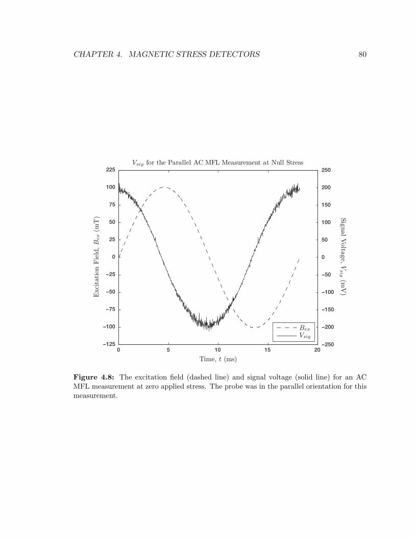
CHAPTER 4. MAGNETIC STRESS DETECTORS 80
0 5 10 15 20−125
−100
−75
−50
−25
0
25
50
75
100
225
Vsig for the Parallel AC MFL Measurement at Null Stress
Time, t (ms)
−250
−200
−150
−100
−50
0
50
100
150
200
250
Sig
nalV
olta
ge,
Vsig
(mV
)
Exci
tation
Fie
ld, Bex (
mT
)
BexVsig
Figure 4.8: The excitation field (dashed line) and signal voltage (solid line) for an ACMFL measurement at zero applied stress. The probe was in the parallel orientation for thismeasurement.

CHAPTER 4. MAGNETIC STRESS DETECTORS 81
therefore fit amplitude was taken as the AC MFL signal voltage, giving
VACM = Af (σ). (4.4)
Figure 4.9 shows VACM for both parallel and perpendicular probe configurations
(Bex ‖ σt and Bex ‖ σc respectively). Uncertainty in VACM was determined by the
95% confidence interval of the fit to equation 4.3. Most of the measurements in figure
4.9 agree within error, indicating no significant relationship between VACM and σ
beyond uncertainty. While there may be a trend in the data, it is not one which is
understandable. As such, this method was deemed to be of little use for any practical
application.
4.4.3 SMA
SMA measurements were the most demanding of the three measurement types, in
terms of both the time required to perform each measurement and the amount of
data analysis needed to convert Vsig waveforms to VSMA values. Before unprocessed
Vsig waveforms can be presented, it is necessary to expand on some of Langman’s
work presented in section 2.4.3.
SMA: A Theoretical Development of Angular Dependence
The SMA probe was rotated about a point, thus capturing information regarding the
direction and magnitude of stress6. Langman described the angle between magnetic
fields inside ( ~Bin) and outside ( ~Bout) the sample (designated δ) as a function of the
relative permeabilities along two perpendicular principle magnetic directions (µr1 and
6While AC and DC MFL measurements were recorded with the probe in two different configu-rations (parallel and perpendicular to applied stress), this was done to examine the measurements’sensitivity to compressive stress.
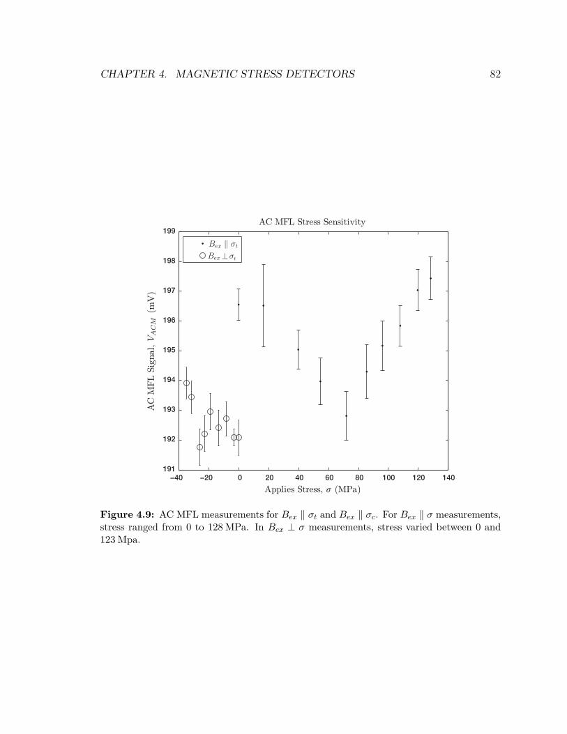
CHAPTER 4. MAGNETIC STRESS DETECTORS 82
−40 −20 0 20 40 60 80 100 120 140
191
192
193
194
195
196
197
198
199AC MFL Stress Sensitivity
AC
MFL
Sig
nal,VACM
(mV
)
Applies Stress, σ (MPa)
t
Figure 4.9: AC MFL measurements for Bex ‖ σt and Bex ‖ σc. For Bex ‖ σ measurements,stress ranged from 0 to 128 MPa. In Bex ⊥ σ measurements, stress varied between 0 and123 Mpa.

CHAPTER 4. MAGNETIC STRESS DETECTORS 83
μ1
μ2
δ
θ
Bin1
Bin2
Bout
Bin
φ
Figure 4.10: A modified figure 2.15 redrawn for reference. The excitation core footprintis indicated by dotted lines.
µr2, with µr2 > µr1), and the angle of the excitation field density relative to the µ2
direction (θ). A modified figure 2.15 is presented here as figure 4.10 for convenient
reference.
In the present application, the direction parallel to applied stress corresponds to
µr2, and µr1 corresponds to the perpendicular direction. Equation 2.27 was given as
δ = arctan
(
(µr2
µr1− 1) tan θ
1 + µr2
µr1tan2 θ
)
.
This equation provided accurate δ values in Langman’s earlier study; however, to use
this equation in its current form requires knowledge of the magnetic field orientation
within the sample, something that is not possible in the present application. However,
it is possible to develop an alternate relationship by expressing θ in terms of φ (recall
that φ is probe angle relative to µr2, indicated in figure 4.10). A reasonable description
for this relationship was found to be
θ = φ +1
3arctan
(
(µr1
µr2− 1) tan φ
1 + µr1
µr2tan2 φ
)
, (4.5)
based on data presented in figure 2.16 and reference [21]. The relationship between
equation 2.27 and equation 4.5 can be explained by considering the two terms in
equation 4.5 independently.

CHAPTER 4. MAGNETIC STRESS DETECTORS 84
Both ~Bin orientation (θ) and probe orientation (φ) were measured relative to the
µ2 direction, which accounts for the separate φ term in equation 4.5. The arctan(...)
component shifts θ from φ toward µ2. The factor of 1/3 was selected based on the
angles between φ, ~Bin and ~Bout shown in figure 2.16.
The two principle magnetic directions (µr1 and µr2) cause the magnitude of Bout
to depend on the orientation of the internal magnetic field. This relationship can be
expressed as
Bout =
√
(
Bin1
µr1
)2
+
(
Bin2
µr2
)2
. (4.6)
Using equations 2.22 and 2.23, equation 4.6 can be rearranged to
Bout
Bin
=
√
(
sin θ
µr1
)2
+
(
cos θ
µr2
)2
, (4.7)
which gives the magnitude of Bout per unit Bin.
An SMA sensing coil voltage signal will be a function both the magnitude, orien-
tation, and rate of change of ~Bout, as well as probe properties (number of turns and
coil area). Thus the SMA signal voltage in terms of Bin is
V = NAG∂
∂t(Bin) , (4.8)
where the G term is called the ‘geometry factor.’ G compensates for the different
magnitudes and orientations of ~Bin and ~Bout, as well probe orientation. For the SMA
detector described in this thesis, which is a coil rotated 90 from the probe angle φ,
the geometry factor takes the form
G =
[
(
sin θ
µr1
)2
+
(
cos θ
µr2
)2]1/2
sin (θ + δ − φ) , (4.9)
where θ is given by equation 4.5 and δ is determined by equation 2.27, both of which
are functions of probe angle φ. The square-root term, shown in square brackets, gives

CHAPTER 4. MAGNETIC STRESS DETECTORS 85
Geo
met
ry F
act
or,
G
Probe Angle, φ (deg)
0 50 100 150 200 250 300 350
0.3
0.2
0.1
0
-0.1
-0.2
-0.3
μr2/μ
r1 = 2
μr2/μ
r1 = 3
μr2/μ
r1 = 4
μr2/μ
r1 = 1
Figure 4.11: G for four µr2/µr1 ratios. The 0 , 180 , and 360 probe orientations placethe probe parallel to the µ2 direction.
the magnitude of Bout from Bin, it was taken directly from equation 4.7. The sin(...)
term extracts the component of ~Bout parallel to the coil’s axis.
Figure 4.11 shows the geometry factor G over a complete probe rotation (φ = 0 to
360) for several theoretical µr2/µr1 ratios. For the case of µr2/µr1 = 1 the geometry
factor is zero, indicating that isotropic samples would produce no signal in the SMA
coil. Other relative permeability ratios produce sinusoidal, 180 periodic geometry
factors, with amplitude increasing with µr2/µr1. Peak G values occur when the probe
is shifted 45 anti-clockwise from the direction of greatest permeability.

CHAPTER 4. MAGNETIC STRESS DETECTORS 86
SMA Results and Analysis
The excitation field used in SMA measurements was a 55 Hz sine wave with a 100 mT
amplitude, identical to the field used for AC MFL measurements (refer to equation
4.2). Measurements were performed up to a maximum sample tensile stress of 130
MPa.
For each SMA measurement the probe was rotated 360 in 15 increments, with
Vsig waveforms collected for each increment. Vsig waveforms, functions of both stress
(σ) and probe orientation (φ), were fit in MATLAB R© to the equation
Vsig(σ, φ) = Af (σ, φ) sin(2πt55 Hz + Bf ) + Cf , (4.10)
where Cf is fit offset, Bf is fit phase, and Af (σ, φ) is fit amplitude, which was expected
to be a function of both applied stress and probe angle. Both offset and phase were
expected to be constant.
Figure 4.12 shows Af (σ, φ) for four stress levels (σ = 0 MPa, 61.6 MPa, 97.7 MPa,
129 MPa). Uncertainty values were taken as the 95% confidence intervals of the fit.
The effects of stress on Af (σ, φ) can be seen in the first 90of rotation, where the signal
follows an inverted sinusoidal line for σ = 0 MPa, decreases in amplitude as stress
increases to σ = 61.6 MPa, then inverts to a standard sine waveform at σ = 97.7 MPa,
and finally increases in amplitude for σ = 129 MPa.
Based on the amplitude of Af (σ, φ) and anisotropy analysis presented earlier in
this section, it can be seen that the initial bulk magnetic easy axis of the sample is in
the perpendicular direction7, which agrees with previous studies performed in these
plates [24]. Increasing tensile stress along the parallel direction causes a corresponding
7Recall that peaks in the anisotropy signal occur 45 anti-clockwise from the direction of greatestpermeability.

CHAPTER 4. MAGNETIC STRESS DETECTORS 87
−50 0 50 100 150 200 250 300 350 400
95
100
105
110
115
95
100
105
110
115
95
100
105
110
115
95
100
105
110
115
SMA Vsig(σ, φ) Amplitude for Bex = 100 mT sin(2πt55 Hz)
Fit
Am
plitu
de,
Af(σ,φ)
(mV
)
Angle, φ (deg)Probe
σ = 0 MPa
σ = 61.6 MPa
σ = 97.7 MPa
σ = 129 MPa
Figure 4.12: Vsig(σ, φ) fit amplitudes for SMA measurements. Each data set consists of 25points recorded at 15 intervals between 0 and 360. 0 , 180 , and 360 probe orientationsplaced the probe (and excitation field) parallel to the applied stress.

CHAPTER 4. MAGNETIC STRESS DETECTORS 88
increase in magnetic permeability, bringing the sample close to an isotropic state for
σ = 66.1 MPa. At σ = 91.7 MPa, the easy axis has shifted to the parallel orientation.
To arrive at VSMA, the Vsig amplitude waveforms shown in figure 4.12 were fit to
a 180-periodic sine function according to
Af (σ, φ) = Af2(σ) sin
(
2π
180φ + Bf2
)
+ Cf2. (4.11)
As with the initial fit (see equation 4.10), the phase (Bf2) and offset (Cf2) parameters
were expected to be constant: though they were fit in MATLAB, they were confirmed
to remain relatively constant. The amplitude was expected to be proportional to the
stress applied to the sample, thus
VSMA = Af2(σ). (4.12)
Figure 4.13 shows the SMA signal voltage (VSMA) obtained from fits to equation
4.11. The data shows a linear increase in SMA signal amplitude with applied stress
and sufficiently low uncertainties for data points to be clearly distinguished. The
‘initial measurement’ data set corresponds to the data presented earlier in figure 4.12.
The ‘repeated measurement’ data set was acquired after the initial measurement at
approximately equivalent applied stress levels. Between measurements the probe
was removed from the sample and replaced at the same location. The purpose of
the repeated measurement was to evaluate the repeatability of SMA measurements.
The two data sets agree within uncertainty, although the repeated measurement has
consistently higher uncertainty than the initial measurement.

CHAPTER 4. MAGNETIC STRESS DETECTORS 89
−20 0 20 40 60 80 100 120 140
−15
−10
−5
0
5
10
15
Applied Stress, σ (MPa)
SM
ASig
nalV
olt
age,
VSMA
(mV
)
Anisotropy Signal from a Mild Steel Plate
initial measurement
repeated measurement
Figure 4.13: SMA measurements for tensile up to 130 MPa.

CHAPTER 4. MAGNETIC STRESS DETECTORS 90
4.5 Selected Detector
Of the three detectors tested, only the AC MFL coil demonstrated no stress sensitiv-
ity. This could have been due to the apparatus or data processing methods, as the
measurement was of the same nature as DC MFL tests.
DC MFL measurements behaved generally as expected: VDCM decreased with the
probe parallel to tensile stress, and increased with the probe oriented along com-
pressive stress. However, significant scatter in the data suggested that quantitative
measurements may be difficult with a DC MFL-based probe.
The SMA detector indicated a strong relationship between applied stress and both
the initial measurement (as Af (σ, φ)), as well as the VSMA value. SMA measurements
are also capable of providing additional information about the orientation of stresses
within the sample, and were demonstrated to be repeatable. For these reasons, an
SMA sensing coil was selected as the magnetic flux transducer for the second probe
design.

Chapter 5
Proposed Design: The Magnetic
Anisotropy Prototype Probe
Previous chapters described the testing of different feedback systems and sensor con-
figurations with a general-use excitation core. The general-use core was relatively
large (the pole area was 264 mm2 with a back spine length of 64 mm) and was tested
on flat plate samples. This chapter describes the features of a prototype probe devel-
oped specifically for use on CANDUR© feeders, termed the Magnetic Anisotropy Pro-
totype (MAP) probe, that combined a smaller, Supermendur-cored excitation core
with the FCV2 flux control system and an SMA detector coil. Section 5.1 outlines
the design characteristics of the MAP probe, while section 5.2 describes experiments
conducted on a section of pipe similar to the feeders found in CANDU R© reactors.
91

CHAPTER 5. PROPOSED DESIGN: MAP PROBE 92
5.1 Magnetic Anisotropy Prototype (MAP) Probe
The optimized probe for stress measurement in feeders, termed the Magnetic Anisotropy
Prototype probe (MAP probe), consisted of a Supermendur1 U-core excitation elec-
tromagnet coupled with a 200 turn SMA coil. A BH-700 feedback Hall sensor and
a feedback coil were integrated into the MAP probe so that it could be used with
FCV2. It should be noted that the MAP probe will not fit within the clearances of a
CANDU reactor face: it is too tall. However, the components selected for the probe
were chosen so that modification to certain parts, such as the connector assembly,
would allow the system to be used in a CANDUR© feeder pipe environment.
The Supermendur core, shown in figure 5.1, consists of thin layers of a 49% Co,
49% Fe, 2% V alloy. The layers are held together with a non-conductive epoxy that
limits the formation of eddy currents, which decreases power loss within the core,
making it ideal for AC magnetic applications. The core is small, with a height of
15.76 mm and a footprint of 38.18 mm2, and was integrated into a housing assembly
appropriate for SMA measurements.
The MAP assembly, shown in figure 5.2(a), was built around the Supermendur
core. For the probe to function with FCV2, a feedback Hall sensor, feedback coils and
excitation coils were mounted to the core. These coils, and other important MAP
components are shown in figure 5.2. The connector brace, shown in white, fits tightly
into a stainless steel disk (shown in figure 5.2 (b)) which is free to rotate in a larger
aluminum mount that can be clamped to samples.
1‘Supermendur’ is the product name of a discontinued layered magnetic alloy from Carpenter
Technologies.
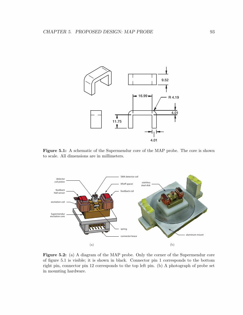
CHAPTER 5. PROPOSED DESIGN: MAP PROBE 93
4.01
16.99
11.75
4.01
9.52
R 4.19
Figure 5.1: A schematic of the Supermendur core of the MAP probe. The core is shownto scale. All dimensions are in millimeters.
aluminum mount
stainless
steel disk
feedback coil
excitation coil
SMA detector coil
feedback
Hall sensor
connector brace
spring
lifto! spacer
Supermendurexcitation core
detector
coil piston
(a) (b)
Figure 5.2: (a) A diagram of the MAP probe. Only the corner of the Supermendur coreof figure 5.1 is visible; it is shown in black. Connector pin 1 corresponds to the bottomright pin, connector pin 12 corresponds to the top left pin. (b) A photograph of probe setin mounting hardware.

CHAPTER 5. PROPOSED DESIGN: MAP PROBE 94
Excitation and feedback coils were wound using MWS Wire Industries PN Bond2
magnet wire and placed on each pole of the excitation core. A thin layer of Teflon tape
was placed between the core and coils to protect the coils; it appears as a white band
between the feedback coils and liftoff spacers in figure 5.2. Both the excitation and
feedback coils were wound in pairs: the excitation system was made of two 36 AWG
250 turn coils, the feedback system consisted of two 36 AWG 25 turn coils. Excitation
and feedback coils were placed on each pole of the excitation and connected in series
effectively creating one 500 turn excitation coil and one 50 turn feedback coil (from
this point onward these coils will be referred to in the singular). The SMA detector
coil was mounted in a spring-loaded piston to ensure repeatable SMA coil coupling
with the sample. The SMA coil used in the MAP probe was 200 turns, wound out of
44 AWG PN bond wire around a ferrite core. Table 5.1 summarizes the properties of
the excitation, feedback and SMA coil properties used in the MAP probe.
The SMA coil was encased in epoxy within a plastic piston assembly. As mentioned
previously, a small spring (Gardner Spring part 36000G) pushes against the back of
the piston to ensure repeatable detector coil coupling to the sample. The piston is
housed in a brass mounting bracket that connects it to the Supermendur core and
connector brace.
The connector brace was machined out of plastic and contained 12 pin Tyco Elec-
tronics AMP male connector. The connection diagram for this terminal is given in
figure 5.3.
2PN Bond wire is an insulated copper wire with a superimposed film of thermoplastic bondingmaterial. Heat or solvent will cause the bonding layer to soften and fuse layers of wire together.This allows coils to be wound in unusual shapes or on jigs since the coils are bonded turn to turn.

CHAPTER 5. PROPOSED DESIGN: MAP PROBE 95
excitation coil
turnstwo 250 turn coils in series
2 × 250 = 500resistance 23.5 Ωwire gage 36 AWG PN Bond
core material Supermendurcoil area 4.5 mm × 10 mm = 45 × 10−6 m2
feedback coil
turnstwo 25 turn coils in series
2 × 25 = 50resistance 2.15 Ωwire gage 36 AWG PN Bond
core material Supermendurcoil area 4.5 mm × 10 mm = 45 × 10−6 m2
anisotropy coil
turns one 200 turn coilresistance 16.9 Ωwire gage 44 AWG PN Bond
core material Ferritecoil area 2 mm × 2 mm = 4 × 10⁻⁶ m2
Table 5.1: MAP probe properties. Feedback and excitation coils were wound on anexternal forming rig, which is why their area differs from the Supermendur core footprint.
1
12
1
2
3
4
5
6
7
8
9
10
11
12
VH-VH+
-Ic+Ic
Vex-Vex-
Vfc+Vfc-
NCNC
Vsig+Vsig-
Figure 5.3: The pin diagram for the MAP system. NC indicates no connection at thatterminal.

CHAPTER 5. PROPOSED DESIGN: MAP PROBE 96
5.2 MAP Probe Testing with SA-106 Grade B Pipe
To evaluate the stress sensitivity of the MAP probe, it was clamped to a length of
2.5 inch nominal diameter SA-106 grade B pipe mounted in a three-point bending rig
(3PBR). The bending rig and sample are described in section 5.2.1, while results are
given in sections 5.2.2 and 5.2.3.
5.2.1 The Three-Point Bending Rig (3PBR) and SA-106 Grade
B Sample
The Three-Point Bending Rig (3PBR), shown in figure 5.4, was designed by Steven
White to apply compressive and tensile axial loads to a 3.18 m long, 2.5 inch nominal
diameter Schedule 80 SA-106 grade B pipe, hereafter referred to as the SA-106 sample,
using three 6 ton bottle jacks mounted on a steel I-beam. The top of the pipe directly
above the middle jack was taken as the surface origin (0 cm, 0) in (axial, hoop)
coordinates, according to the coordinate system indicated in figure 5.4.
The application of tensile and compressive axial (σa) loads required different tow-
ing strap configurations. In the tensile configuration, shown in figure 5.4, the SA-106
sample was strapped at its ends and a tensile axial stress state (σa > 0) at the
measurement location (top surface) was achieved by raising the middle jack. In the
compressive configuration (not shown) the pipe was strapped at the center with two
towing straps. Compressive axial stress (σa < 0) was applied by raising the two outer
jacks. Hoop stress (σh) was generated for both configurations by Poisson effects.
Four Vishay R© EA-06-250BF350 general purpose 350Ω strain gages with gage fac-
tors of 2.100 ± 0.5% and a transverse sensitivy of 0.0 ± 0.5% were mounted to the
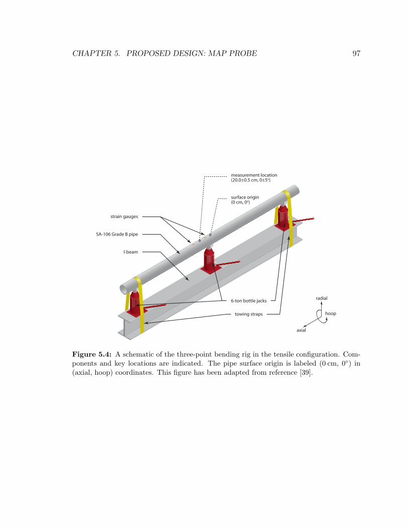
CHAPTER 5. PROPOSED DESIGN: MAP PROBE 97
radial
hoop
axial
6-ton bottle jacks
towing straps
I-beam
SA-106 Grade B pipe
surface origin(0 cm, 0o)
strain gauges
measurement location(20.0±0.5 cm, 0±5o)
Figure 5.4: A schematic of the three-point bending rig in the tensile configuration. Com-ponents and key locations are indicated. The pipe surface origin is labeled (0 cm, 0) in(axial, hoop) coordinates. This figure has been adapted from reference [39].

CHAPTER 5. PROPOSED DESIGN: MAP PROBE 98
sample to measure hoop and axial strain. The two axial strain (εa) gages are centered
at (9.1 cm, 0) and (30.2 cm, 0). The two remaining gages are oriented to meausre
hoop strain (εh) and are centered at (11.5 cm, 0) and (28.5 cm, 0). The surface of
the pipe surrounding and between the strain gages was sanded to a smooth finish to
allow proper gage mounting. The strain gages were connected to a Vishay R© Measure-
ments Group SB-10 Balance and Switch for calibration and switching. The SB-10
was connected to a Vishay R© Measurements Group P3500 Strain Indicator.
SA-106 grade B piping has a minimum specified yield strength of 240 MPa, a
Young’s modulus of Y = 202.7 GPa at 21 C and a Poisson’s ratio of ν = 0.3 [1], [39].
The generalized form of Hooke’s law for an isotropic material (refer to equation 2.3)
in cylindrical coordinates gives the axial stress (σa) as
σa =Y
1 + ν
[
εa +ν
1 − 2ν(εa + εh + εr)
]
, (5.1)
and hoop stress (σa) as
σh =Y
1 + ν
[
εh +ν
1 − 2ν(εa + εh + εr)
]
, (5.2)
where εr is radial strain. No strain gage was mounted to record εr; however, previous
neutron diffraction studies have shown it to be small compared to εa and εh [39],
therefore εr = 0 provided a reasonable simplification. εa and εh were recorded by
the axial and hoop strain gages described above. The MAP probe was placed in the
middle of the strain gages at (20.0 ± 0.5 cm, 0 ± 5), indicated in figure 5.4. Linear
interpolation was used to approximate strain at the measurement location.

CHAPTER 5. PROPOSED DESIGN: MAP PROBE 99
5.2.2 SMA Excitation Field Response
The 3PBR was used to characterize MAP anisotropy signal excitation field response.
The MAP probe was mechanically clamped to the SA-106 sample at (20.0 ± 0.5 cm,
0 ± 5) in (radial, hoop) coordinates and the pressure valves of each jack in the
3PBR was released, bringing the system to a zero applied stress state. Excitation
waveforms used with the MAP probe were sinusoidal with amplitude A and frequency
f , described by:
Bex = A sin (2πf) . (5.3)
The excitation frequency f affects two parameters of the SMA signal: amplitude and
skin depth. As with any wire coil, SMA signal amplitude increases with the time-
rate of change of the detected field (∂Bex/∂t). Skin depth (δ) refers to the depth to
which an electromagnetic field propagates within a conductor, and is defined as the
distance at which wave amplitude decreases to 1/e ≈ 0.368 of the value at the sample
surface. This attenuation is caused by ohmic losses within the conductive medium
and is discussed in detail in appendix B. Skin depth for a typical ferromagnetic steel
is given by:3
δ = 1.59 × 10⁻²m.s0.5√
f. (5.4)
An excitation frequency of f = 55 Hz gives a skin depth of δ = 2.15 mm. The
magnetic field is 95% attenuated at 3δ = 6.45 mm, which covers the majority of the
7.01 mm pipe wall thickness of the SA-106 sample. Lower frequencies would penetrate
deeper into the sample, but produce lower amplitude voltage response in the SMA
detector coil. An excitation frequency of f = 55 Hz was found to provide a good
3Assuming a conductivity (σe) of σe = 107 Ω−1m−1, and a relative permeability of µr = 100.

CHAPTER 5. PROPOSED DESIGN: MAP PROBE 100
0 20 40 60 80 100 120 1400
20
40
60
80
100
120
140
160
180
SA-106 Sample Anisotropy
Excitation Field Amplitude, A (mT)
SM
ASig
nalV
olt
age,
VSMA
(mV
)
0 20 40 60 80 100 120 1400
1
2
3
4
5
6
7
8
SA-106 Sample Signal Error to Signal Ratio
Excitation Field Amplitude, A (mT)
(a) (b)
Per
cent
Unce
rtai
nty
(%
)
Figure 5.5: SMA dependence on excitation field amplitude for σa = 0. VSMA was calcu-lated using the same method described in section 4.4. (a) The anisotropy signal VSMA. (b)The percent error associated with each measurement.
balance of penetration and signal amplitude.
The relationship between SMA signal voltage (VSMA) and excitation field ampli-
tude (A) was characterized by performing SMA measurements with the MAP probe
on the SA-106 sample at excitation field amplitudes varying from A = 25 mT to
125 mT in in 25 mT increments. The maximum excitation field amplitude of 125 mT
was determined by the current capacity of the 36 AWG excitation coils used in the
MAP probe. The results are presented in figure 5.5 (a), were it can be seen that VSMA
increases relatively linearly with A. The explanation for this relationship is simple:
the magnetic flux detected by the SMA coil is a relatively constant fraction of the
total magnetic flux in the system.
The percent uncertainty associated with each VSMA measurement, determined

CHAPTER 5. PROPOSED DESIGN: MAP PROBE 101
by the 95% confidence interval of the fit (as described in section 4.4), is shown in
figure 5.5 (b). The percent uncertainty decreases from low excitation field values to
a minimum of 3.5% at A = 100 mT, then increases for A = 125 mT. Because of
the slight difference in uncertainties between 75 mT and 100 mT excitation fields, an
excitation field amplitude of A = 75 mT was used for measurements on the 3PBR.
5.2.3 SA-106 Grade B SMA Stress Response
The stress response of the MAP sensor configured as described in section 5.2.2, with a
55 Hz, 75 mT excitation field, are shown in figure 5.6 (a) for tensile stress. The back-
ground measurement at σa = 0 MPa agrees within error to that presented in figure
5.5. As shown in figure 5.6, increases in axial tension were accompanied by increases
in VSMA, but the observed VSMA changes were small and the four different Vsig(σa, φ)
waveforms shown in figure 5.6 (b) are difficult to distinguish, unlike previous SMA
results presented in figure 4.12. The probe was aligned with angles φ = 0, 180, 360
along the pipe axis (parallel to σa), and φ = 90, 270 along the pipe hoop (parallel to
σh). The results in figure 5.6 (b) indicate an initial easy axis along the axial direction
which increases in permeability with σa.
Additional MAP Probe Modifications
Initial MAP results were less stress-sensitive than desired. Minor modifications were
made to the SMA coil mount and liftoff pads in an attempt to increase sensitivity
and decrease measurement uncertainty. Movement of the sensor during measurements
was believed to contribute to inconsistent coil coupling, which increased measurement
uncertainty. To counteract this effect, a piece of electrical tape (0.36 mm thick) was

CHAPTER 5. PROPOSED DESIGN: MAP PROBE 102
−20 0 20 40 60 80
85
90
95
100
105
110
2.5” SA-106 Grade B Anisotropy Signal
Axial Stress, σa(MPa)
SM
ASig
nalV
olt
age,
VSMA
(mV
)
−100 0 100 200 300 400
−150
−100
−50
0
50
100
150
SMA Vsig(σ ,φ) Amplitude
Probe Angle, φ (deg)
Fit
Am
plitu
de,
Af(σ
,φ)
(mV
)
(a) (b)
= 0 MPa
= 16.3 MPa
= 45.8 MPa
= 67.3 MPa
σa
σa
σa
σa
σa
a
Figure 5.6: MAP stress response for an excitation field Bex = 75 mT sin(2πt55 Hz). (a)VSMA values. (b) The Vsig(σa, φ) values for each probe orientation. Error bars are omittedfor clarity.

CHAPTER 5. PROPOSED DESIGN: MAP PROBE 103
placed between the SMA detector coil and sample to provide more consistent coupling
between the detector coil and sample. Liftoff spacer thickness was slightly reduced
to ease the current burden of the excitation coils.
Modified MAP Results and Analysis
The modified MAP was tested with the same excitation field as the original design.
With the 3PBR in the tensile configuration, axial tensile stresses were varied from 0 to
270 MPa. The 3PBR was then configured to apply compressive stress to the SA-106
sample, and compressive stresses were varied from 0 to -68 MPa. Measurements were
performed by recording Vsig(σa, φ) waveforms for φ = 0 to φ = 360 in 15increments.
Stress test results from the modified MAP are presented in figure 5.7. The initial
increasing tensile stress measurement results in an increasing VSMA, while compressive
stress produce a decrease in VSMA. The background readings (σa = 0) for both
measurements agree within error.
Tensile and compressive MAP data was evaluated with a linear least-squares fit,
producing
VSMA(mV) = 0.183σa(MPa) + 69.9 (5.5)
as the line of best fit. This linearization is also shown in figure 5.7. All data points
agree with the linear fit within uncertainty; however there does appear to be slight
oscillatory trend about the line of best fit.
The mean uncertainty in MAP probe SMA measurements was found to be ±7 mV,
with a minimum uncertainty of ±5 mV and a maximum uncertainty of ±10 mV. Solv-
ing equation 5.5 for σa indicates that a ±7 mV uncertainty in VSMA corresponds to a
±38 MPa uncertainty in stress. Therefore the current MAP probe can evaluate elastic

CHAPTER 5. PROPOSED DESIGN: MAP PROBE 104
−100 −50 0 50 100 150 200 250 30050
60
70
80
90
100
110
120
1302.5” SA-106 Grade B Anisotropy Signal
Axial Stress, σa(MPa)
SM
ASig
nalV
olt
age,
VSMA
(mV
)
tensile
compressive
linear fit
Figure 5.7: SMA dependence on tensile and compressive applied stress. Vertical dashedlines indicate σa = 0 and σa = 240 MPa.

CHAPTER 5. PROPOSED DESIGN: MAP PROBE 105
−50 0 50 100 150 200 250 300 350 400−100
−80
−60
−40
−20
0
20
40
60
80
SMA Vsig(σa, φ) Amplitude
Probe Angle, φ (deg)
Fit
Am
plitu
de,
Af(σa,φ
)(m
V)
σaσa
= 47 MPa
= -44 MPa
Figure 5.8: Signal voltage Vsig(σa, φ) fit amplitude for approximately equivalent compres-sive (σa = −44 MPa) and tensile (σa = 47 MPa) stresses. The uncertainty associated witheach data point is smaller than the data marker.
stress in feeders from VSMA values with an accuracy of approximately ±38 MPa.
It was observed that the uncertainty associated with compressive measurements
was, in general, much larger than the uncertainty of equivalent tensile measurements.
Figure 5.8 shows the signal voltage amplitude (Af (σa, φ)) for σa = 47 MPa and σa =
−44 MPa. There is only a small difference in amplitude between the two stress levels
at φ = 45 and φ = 315 , approximately 3 mV; however Af (−44MPa, φ = 135, 225)
is approximately 20 mV less than Af (47 MPa, φ = 135, 225). The discrepancy be-
tween peak Af (σa, φ) values was the primary cause of the increased uncertainty as-
sociated with compressive measurements.
The SMA detector coil of the MAP probe was irreparably damaged while inves-
tigating the cause of the compressive measurement peak distribution, ending data

CHAPTER 5. PROPOSED DESIGN: MAP PROBE 106
collection with this probe.

Chapter 6
Summary and Conclusions
Residual stress measurement is a priority for industries where the cost of failure
is significantly greater than the cost of regular inspection. A technique based on
stress-induced magnetic anisotropy (SMA) may present a viable method for in situ
residual stress measurement on components where tight clearances and varying sur-
face conditions hinder other stress measurement methods. This thesis focused on the
development of hardware, software and signal analysis methods necessary to apply
SMA measurement to SA-106 Grade B feeder pipes used in CANDU R© nuclear reac-
tors. In this chapter the success of this project will be evaluated based on the project
objectives specified in section 1.3.
6.1 Flux Control Systems
Two magnetic flux control systems, FCV1 and FCV2, were designed to compensate
for geometry effects resulting from the curved surface of a pipe wall. FCV1 relied
exclusively on feedback from a Hall sensor located between the sample and excitation
107

CHAPTER 6. SUMMARY AND CONCLUSIONS 108
core. This control system was found to be unstable due to the nature of the feedback
path.
The second flux control system (FCV2) was designed with two feedback mecha-
nisms: a wire coil (called the feedback coil) wound around the base of the excitation
core, and a Hall sensor (called the feedback Hall sensor) fixed between the excitation
core and sample. The hardware control system of FCV2 compared the magnetic flux
density at these two points with a user-defined reference value, and adjusted the exci-
tation voltage (the voltage across the excitation coil) to produce the desired magnetic
field.
The software requirements of FCV2 were implemented in LabVIEW R© . A program
was designed to calculate reference waveform parameters (Vref ) from a user-specified
excitation magnetic field (Bex). This software was also used for data acquisition and
output via a PCI-6229 DAQ.
FCV2 fulfills a portion of the first project objective, which was to “design a
magnetic flux leakage-based probe that can accommodate the space and geometry
(lift-off) constraints imposed by the feeder pipe environment.”
6.2 Magnetic Stress Detectors
Three magnetic stress detectors were tested on mild steel plate samples with a pro-
totype excitation core controlled by FCV2. Each detector was designed to function
somewhat differently: a Hall sensor was used with DC excitation fields (DC MFL), a
wire coil was used with AC excitation fields (AC MFL), and a specially oriented coil
was used in anisotropy measurements (SMA). The AC MFL measurement showed
no significant stress sensitivity. DC MFL measurements indicated a stress dependent

CHAPTER 6. SUMMARY AND CONCLUSIONS 109
trend, but significant scatter would have made it problematic for quantitative stress
measurement.
SMA measurements were the most time-intensive to perform, requiring a full probe
rotation per measurement, and the most computationally intensive to analyze. How-
ever, flat plate tests indicated that this measurement was significantly more sensitive
to stress than the others. Because of the high stress sensitivity SMA measurements
were selected as the most likely candidate to produce reasonable stress measurements
from SA-106 grade B feeder pipes, and a prototype SMA-based probe (the Magnetic
Anisotropy Prototype probe) was designed accordingly.
The flat plate magnetic stress detector tests were carried out to complete the
second project objective: to “conduct laboratory testing on plate samples to determine
the extent of stress sensitivity of the probe designs.”
6.3 Proposed MAP Probe Design
The Magnetic Anisotropy Prototype (MAP) probe - a small Supermendur excitation
coil coupled with a ferrite core SMA coil and FCV2 compatible feedback components
- was designed specifically for use on CANDU R© feeder pipes. The probe was designed
to rest in a brace clamped to the sample, where it could be rotated about a point to
perform an anisotropy measurement.
MAP stress sensitivity was examined in tensile and compressive stress tests using
the three-point bending rig and a 2.5” nominal diameter SA-106 grade B pipe sam-
ple. While the stress-induced magnetic anisotropy signal voltage (VSMA) recorded
in MAP measurements indicated clear stress dependence, the uncertainty associated
with MAP VSMA indicate that the probe is not yet suited for industrial use. MAP

CHAPTER 6. SUMMARY AND CONCLUSIONS 110
testing completed objective three, which was to “conduct testing on samples with
feeder pipe geometry with a focus on generalized stresses.”
6.4 Recommendations for Future Work
There are several aspects of this project that could be developed further. Section 6.4.1
details how certain project objectives could be brought to completion and section 6.4.2
examines additional work that could improve both FCV1 and FCV2. Section 6.4.3
suggests a new probe design that may yield improved results.
6.4.1 Project Objectives
Not all of the project objectives outlined in section 1.3 were fully met. Many of the
shortcomings of this project result from the MAP, either by virtue of design or due
to the sudden failure of its SMA coil.
Project objective one was to “design a magnetic flux leakage-based probe that can
accommodate the space and geometry (lift-off) constraints imposed by the feeder pipe
environment.” FCV2 fulfilled a portion of that requirement by providing a method of
coupling a consistent and repeatable flux into the sample, as discussed in section 6.1.
However, the rest of the objective was not met: the MAP probe will not fit within the
confines of a CANDU R© reactor face due to the connector brace and manual rotation
of the probe. Some modifications to the MAP design would meet this objective, such
as a redesigned connection system and a servo-based mechanical rotation system, but
this was not explored further in this project.

CHAPTER 6. SUMMARY AND CONCLUSIONS 111
Project objective three was to “conduct testing on samples with feeder pipe geom-
etry with a focus on generalized stresses.” While this objective was already described
as completed, it would have been beneficial to perform further measurements at dif-
ferent excitation frequencies to extract additional depth information.
The fourth objective was to “conduct testing on feeder pipe samples.” This ob-
jective was not met due to failure of the SMA stress detection coil in the MAP. The
detection coil was 200 turns, wound out of 44 AWG wire around a ferrite core. Fail-
ure occurred when the wires connecting the coil to the connector brace snapped. The
break occurred at the edge of the epoxy encasing the SMA coil and could not be
repaired, ending data collection. This objective could be completed by rebuilding the
MAP probe SMA coil.
6.4.2 Control Systems
While some justifications of the shortcomings of FCV1 and the success of FCV2
are presented in section 3.5.4, a detailed control-theory analysis of both FCV1 and
FCV2 would yield further information about the noise observed in FCV1 and the
performance limits of FCV2. It is also possible that additional analysis of FCV1 may
yield information relating to possible modifications that would produce a functioning
Hall sensor feedback system.
6.4.3 Suggested Design Modifications
The objective of this work was to develop a magnetic stress inspection system that
could be used as an early prototype for an industrial CANDUR© feeder pipe inspection
technology. One of the difficulties of designing a system for use at a CANDU R© reactor

CHAPTER 6. SUMMARY AND CONCLUSIONS 112
y core
x core
excitation coil
feedback coil
sample
(a)
4
detector coil1
2
3
coil mount4
(b)
Figure 6.1: The recommended system for future work. (a) Two perpendicular U-corescan rotate the magnetic field at their center by adjusting the excitation field generated byeach core. Adapted from [39]. (b) The recommended anisotropy coil configuration for atetrapole excitation system. Coils 1 and 3 are connected in series, as are coils 2 and 4.
face is accessibility: an elaborate network of coolant feeders with a minimum inter-
pipe clearance of 20 mm make it difficult for operators and tools to reach inspection
locations. The design presented in chapter 5 does not fit within the clearances of
CANDU R© feeder pipes and requires manual rotation. To overcome both of these
issues, a four pole excitation system (termed a tetrapole system) such as the the
spring-loaded tetrapole prototype (SL4P) designed by Steven White for magnetic
Barkhausen noise measurements [39], could be used to generate the excitation field.
The SL4P consists of two Supermendur U-cores oriented perpendicular to one another,
as shown in figure 6.1 (a), and can rotate the magnetic field at the center of the cores
by superimposing different excitation field amplitudes in the x and y cores. An
anisotropy coil, shown in figure 6.1 (b), consisting of four wire coils could be used
to detect the anisotropy signal. The coils would be connected in pairs (1 to 3 and
2 to 4), and the anisotropy signal would be taken as the quadrature sum of the coil
voltages. This tetrapole probe design would potentially enable measurements to be
made on feeder pipes without the need for manual probe rotation.

Bibliography
[1] 2004 ASME Boiler and Pressure Vessel Code, Section IIA. Ferrous Material
Specifications. American Society of Mechanical Engineers, 2006.
[2] D.L. Atherton A. Dhar, L. Clapham. Influence of uniaxial plastic deformation on
magnetic barkhausen noise in steel. NDT & E International, 34:507–514, 2001.
[3] N. Akulov. Zur atomtheorie des ferromagnetismus. Zeitschrift fur Physik A
Hadrons and Nuclei, 54:582–587, 1929.
[4] H. Barkhausen. Zwei mit hilfe der neuen verstarker entdeckte erscheinugen.
Zeitschrift fur Physik, 20:401–403, 1919.
[5] L. Clapham C. Mandache, T.W. Krause. Investigation of optimum field ampli-
tude for stress dependence of magnetic barkhausen noise. IEEE Transactions on
Magnetics, 43(11):3976–3983, 2007.
[6] S. Chikazumi. Physics of Magnetism. John Wiley & Sons, 1964.
[7] B.D. Cullity. Introduction to Magnetic Materials. Addison-Wesley, 1972.
[8] B. Drafts. Understanding Hall Effect Divices. Sypris Test & Measurement,
November 2007.
113

BIBLIOGRAPHY 114
[9] F.W. Bell, a division of Sypris Test & Measurement,
http://www.sypris.com/test-and-measurement/magnetics-fw-bell/fw-bell-
products. F.W. Bell Hall Sensor Catalog, 2007.
[10] S. Zapperi G. Durin. The Barkhausen effect. arXiv:cond-mat/0404512v1, April
2004.
[11] W.J. Garland. How and Why is CANDU Designed the Way It is.
http://canteach.candu.org/library/20000101.pdf, 2003.
[12] D.J. Griffiths. Introduction to Electrodynamics. Prentice Hall, 3 edition, 1999.
[13] E. Hall. On a new action of the magnet on electric currents. American Journal
of Mathematics, 2(3):287–292, 1879.
[14] W. Heisenberg. Mehrkorperproblem und resonanz in der quantenmechanik.
Zeitschrift fur Physik, 38:411–426, 1926.
[15] W. Heisenberg. Zur theorie des ferromagnetismus. Zeitschrift fur Physik, 49:619–
636, 1928.
[16] T.Vigalsky J.C. Jin, A. Blahoianu. Service Induced Degradations of CANDU
Feeder Piping: FAC Wall Thinning and Cracking. International Atomic Energy
Agency, 2006.
[17] D.C. Jiles. Dynamics of domain magnetization and the barkhausen effect.
Czechoslovak Journal of Physics, 50(8):893–988, 2000.
[18] J.P. Joule. On a new class of magnetic forces. The Annals of Electricity, Mag-
netism and Chemistry; and Guardian of Experimental Science, 8:219, 1842.

BIBLIOGRAPHY 115
[19] Thomas W. Krause, L. Clapham, Andras Pattantyus, and David L. Atherton.
Investigation of the stress-dependent magnetic easy axis in steel using magnetic
barkhausen noise. Journal of Applied Physics, 79(8):4242–4252, 1996.
[20] R. Langman. Measurement of the mechanical stress in mild steel by means of
rotation of magnetic field strength. NDT Int., 12:255–262, 1981.
[21] R. Langman. Prediction and measurement of rotation of magnaetization in an
anisotropic polycrystalline ferromagnetic material. IEEE Transactions on Mag-
netics, 17(1):1159–1168, 1981.
[22] R. Langman. Measurement of the mechanical stress in mild steel by means of
rotation of magnetic field strength - part 3: practical applications. NDT Int.,
16:59–66, 1983.
[23] R.A. Langman. Measurement of the mechanical stress in mild steel by means of
rotation of magnetic field strength - part 2: biaxial stress. NDT Int., 15:91–97,
1982.
[24] C. Mandache. Magnetic Flux Leakage Investigation of Interacting Defects: Stress
and Geometry Effects. Queen’s University, 2003.
[25] K. Marble. Investigation of the Magnetic Flux Leakage Signatures of Dents and
Gouges. Queen’s University, 2009.
[26] B. Augustyniak M.J. Sablik. Magnetic methods of nondestructive evaluation,
the wiley encyclopedia of electrical and electronics engineering, 1999.

BIBLIOGRAPHY 116
[27] T.M. Holden T. Lorentzen M.T. Hutchigs, P.J. Withers. Introduction to the
Characterization of Residual Stresses by Neutron Diffraction. Taylor & Francis
Group, 2005.
[28] National Instruments Corporation, www.ni.com. NI 622x Specifications, 2006.
[29] National Instruments Corporation, www.ni.com. DAQ M Series: M Series User
Manual, 2007.
[30] National Semiconductor Corporation, www.national.com. LM137/LM337 3-
Terminal Adjustable Negative Regulators, 2004.
[31] National Semiconductor Corporation, www.national.com. LM4701
OvertureTMAudio Power Amplifier Series 30W Audio Power Amplifier
with Mute and Standby Modes, 2004.
[32] W. Hill P. Horowitz. The Art of Electronic. Cambridge University Press, 1980.
[33] M.A. Plonus. Applied Electromagnetics. McGraw Hill, 8 edition, 1978.
[34] H. Wakiwaka S. Kishimoto, M. Hanabusa and H. Yamada. Conversion theory of
magnetic anisotropy sensor. IEEE Translation Journal on Magnetics in Japan,
(3), 1992.
[35] N. Storey. Electronics: A Systems Approach. Pearson Education Limited, 1998.
[36] J.R. Taylor. An Introduction to Error Analysis. University Science Books, 1996.
[37] C. Hauge P. Weyman B. Sijgers D.L. Atherton T.W. Krause, K. Mandal. Cor-
relation between magnetic flux leakage and magnetic barkhausen noise: Stress

BIBLIOGRAPHY 117
dependence in pipeline steel. Journal of Magnetism and Magnetic Materials,
169:207–219, 1997.
[38] E. Villari. Ueber die aenderungen des magnetischen moments, welche der zug
und das hindurchleiten eines galvanischen stroms in einem stabe von stahl oder
eisen hervorbringen. Annalen der Physik, 202(9):87–122, 1865.
[39] S. White. A Barkhausen Noise NDE System for CANDU R© Feeder Pipes. Queen’s
University, 2009.
[40] G.A. Bickel X.X. Yan, M.D. Pandey. A probabilistic model of wall thinning
in candu feeders due to flow-accelerated corrosion. NuCLear Enigneering and
Design, 238:16–24, 2007.

Appendix A
FCV1 Details
Flux control version 1 (FCV1) was modified several times in attempts to stabilize the
excitation waveform. The basic principle of the control system remained consistent
with that presented in section 3.5; the modifications where capacitors and low-pass
filters that were used to damp out high frequency signals. Figure A.1 shows the
electrical schematic of one of the final iterations of FCV1. Section 3.5 presents data
collected exclusively from this system. Further modification of this design did not
yield significantly improved performance.
118

APPENDIX A. FCV1 DETAILS 119
-
LM4701
+
1
2
3,54
8
7
52 Ω5 W
BH-700
+Ic
-Ic
VH+
VH-
Red
Blu
e
Yell
ow
BlackV
H
1 μF
+24 V
1 μF
-24 V
27 kΩ+24 V
1.2 kΩ 1 kΩ
1 kΩ
1 μF
20 Ω5 W
-
LM747-A
+
13
12
4
2
1
1 μF
-24 V
1 μF
+24 V
-
LM747-B
+10
9
6
7
1 μF
+24 V
1 kΩ
1 kΩ
1 kΩ
1 kΩ
1 kΩ
-
LM747-A
+
13
12
4
2
1
1 μF
-24 V
1 μF
+24 V
1 kΩ
generate ground referenced Hall voltage
Hall sensor current supply
Lex
VH
Vref
-
LM4701
+
1
2
3,54
8
7
1 μF
+24 V
1 μF
-24 V
VsF = 0.5A
0.2 Ω
Rex
Hall voltage comparisonto reference
excitation coil
Figure A.1: An electrical schematic of FCV1. All resistors are 0.25 W unless otherwiseindicated. LM747 op-amps are dual amplifier packages. Different amplifiers within anLM747 are designed A and B.

Appendix B
Skin Depth
Consider a plane electromagnetic wave of magnetic field amplitude B0 incident on a
semi-infinite1 conducting medium of conductivity σe. The amplitude of the magnetic
field within the conductor decreases due to ohmic losses as the wave penetrates fur-
ther in the medium. The term ‘skin depth’ refers to this attenuation, which occurs
according to the exponential law [12]:
B(z) = B0e−z
√πµσef , (B.1)
where B(z) is the amplitude of the wave within the conductor, B0 is the amplitude
of the wave outside the conductor, z represents the direction of propagation, µ is the
permeability of the medium, and f is the frequency of the electromagnetic wave. The
terms in the square root of equation B.1 are rearranged to define the skin depth (δ)
as
δ =
√
1
πσeµf, (B.2)
1Extending from −∞ < x < ∞, −∞ < y < ∞, −∞ < z ≤ 0 in Cartesian coordinates.
120

APPENDIX B. SKIN DEPTH 121
0 20 40 60 80 1000
2
4
6
8
10
Frequency, f (Hz)
Skin
Dep
th,δ
(mm
)
Skin Depth in Generic Steel
12
14
16
Figure B.1: Skin depth for a typical steel with µr = 100 and σe = 107 Ω−1m−1
giving
B(z) = B0e−z/δ. (B.3)
After one δ the amplitude of the magnetic field is reduced by a factor of 1/e. For
most engineering applications, waves are considered to be attenuated at z = 3δ
Figure B.1 shows the variation of skin depth with frequency for a typical steel
with relative permeability of µr ≈ 100 and conductivity σe = 107 Ω−1m−1.