1

A Machine Learning Approach for UnderstandingPower Distribution System Congestion

Emin Ucer∗, Mithat Kisacikoglu∗, Ali Gurbuz†, Shahinur Rahman∗ and Murat Yuksel‡∗Dept. of Electrical and Computer Engineering, The University of Alabama, Tuscaloosa, AL†Dept. of Electrical and Computer Engineering, Mississippi State University, Starkville, MS‡Dept. of Electrical and Computer Engineering, University of Central Florida, Orlando, FL

Emails: eucer@crimson.ua.edu, mkisacik@ua.edu, gurbuz@ece.msstate.edu, srahman6@crimson.ua.edu,murat.yuksel@ucf.edu

Abstract—This study proposes a novel method for learning thecongestion level of the power distribution system which designatesthe loading of a distribution feeder. A machine learning approachis proposed here to find a relating function between substationfeeder power and local voltage. This model is, then, used toestimate real-time substation feeder power consumption usingcurrent local voltage measurements. This fully decentralizedestimation of substation power consumption could facilitate moreelectric vehicle integration into the distribution grid without theneed for real-time centralized control by a system aggregator.The concept is tested with real power loading data of a feederlocated in the state of Alabama. The local voltage measurementdata of a typical house residing in the downstream of the networkof the same feeder is used to develop the learning algorithm.

Index Terms—Machine Learning, Power Distribution System,Electric Vehicles, Congestion

I. INTRODUCTION

Transportation sector is one of the major sources of greenhouse gas emissions. To reduce negative environmental conse-quences of conventional vehicles, transportation electrificationhas been considered as a promising solution [1]. Therefore,electrical vehicle (EV) technology has gained high popularityover the recent years, especially with the introduction of longrange EVs. High penetration of electric vehicles (EVs) withuncontrolled charging is likely to cause transformer and/orline congestion in the power distribution grid. Among someadverse effects of this congestion are severe voltage drops,increased peak loading, thermal overheating, and even failureof equipment [2]–[7]. Congestion in the power distributionsystem is a situation where peak electricity demand nears thesystem capacity. Such a condition may violate thermal limits ofcritical power system components such as feeders and trans-formers. Grid congestion decreases operating efficiency andaffects reliability of the power system. If, for instance, powerlines are congested and operating at or near their thermallimits due to high demand, they will result in significant linelosses [8].

Distribution system operators (DSOs) on the power gridhave to manage congestion on a regular basis [9], [10].Doing this congestion management with low overhead andin a scalable manner for many endpoints with dynamic loadpatterns (e.g., EVs) is a highly needed capability. To this

This material is based upon work supported by the National ScienceFoundation under Award No 1755996.

end, this paper first performs a mathematical analysis of thedistribution system to model the relation between an end-node voltage and total feeder power. In addition, correlationstudies on simulated and experimental data are carried outto validate this relation. Our analysis shows that there is aquasi-linear relation between these variables. There have beensimilar efforts presented in the literature to demonstrate thisrelationship and propose some control solutions. [11] and[12] reveal the strong correlation between grid voltage anddemand power, and propose a plug-and-play controller forhousehold loads in accordance with the grid power demand.[13] demonstrates the voltage-demand relationship in a low-voltage (LV) distribution grid and discusses how this relation-ship can be leveraged for distributed load management. Thevoltage-demand relationship is further exploited and extendedto EV charging control as decentralized solutions with localmeasurements [14], [15]. Voltage droop control is also oftenappealed as a decentralized solution in the distribution grid,particularly for photo-voltaic (PV) integration. [16] appliesthis idea to EV charging control with different droop models.[17] conclude that local control methods allow for a largerEV penetration but are not as capable at maintaining networkparameters within their limits. Authors previously investigatedimpact of EV integration on historical end-node voltage [18]and implemented decentralized controllers that take actionbased on end-node voltages [19], [20].

Unlike the prior works, this study first utilizes the leastsquares estimation method as a machine learning tool. Basedon learning performed on real data, we model this relationshipas a linear function using Linear Regression (LR). Later, toimprove the prediction accuracy and generalize the mappingin case of non-linearity, noise or variation, we build themodel using Gaussian Process Regression (GPR). We furtherimplement a Long-Short Term Memory (LSTM) network tosupport the prediction and compensate for the errors of GPR.These models are learned from substation power data and localvoltage measurements. The innovative aspect of the proposedmethod is to estimate real-time substation total power con-sumption in a fully decentralized way. This decentralizationreduces the need for the end-users to communicate with thesubstation (or centralized server) and enables integration ofhigh-load end-users such as EVs to the grid in a plug-and-play manner. This framework will further help end-users to

2

Figure 1: One-line diagram of a main radial distribution feeder.

efficiently manage their electrical loads locally while main-taining a globally stable grid operation.

The main contributions of our work are as follows:• Analysis and demonstration of the relationship between

end-node voltage and total feeder power based on sim-ulation results and empirical data collected from a realdistribution grid.

• Machine learning (ML) based estimators (LR, GPR, andLSTM) to predict the total feeder power via local end-node voltage measurements.

The rest of the paper is organized as follows: Section IIprovides an analysis for the distribution system operation.Section III explains ML methodologies used in the study.Section IV describes data recording and processing technique.Section V shows the implementation of ML methods andprovides results and discussion. Section V provides the con-cluding remarks and planned future study.

II. ANALYSIS OF THE DISTRIBUTION SYSTEM

A power distribution feeder leave a substation carryingthree-phase power and reduce into single-phase through asingle-phase center-tapped transformer. This transformer pow-ers a group of houses and connects into a household througha single-phase line.

A typical single-feeder radial distribution grid model can beillustrated as in Fig. 1, where Si

L = P iL + jQi

L denotes thecomplex power flowing from node i to node i+1 over a lineimpedance of zi = ri+ jxi. Si

N = P iN + jQi

N is the complexpower drawn from node i, whereas the voltage of ith nodeis denoted by Vi. Then, the distribution model in Fig. 1 canbe recursively solved for any node voltage Vi by using thefollowing DistFlow equations:

P i+1L =P i

L−ri+1P iL2+Qi

L2

V 2i

−P i+1N

Qi+1L =Qi

L−xi+1P iL2+Qi

L2

V 2i

−Qi+1N

V 2i+1=V

2i −2(ri+1P

iL+xi+1Q

iL)+(r2i+1+x

2i+1)

P iL2+Qi

L2

V 2i

(1)

where i = 0, 1, 2, . . . , n [21]. The physics governed by Dist-Flow equations approximates to a linear relationship betweenany end-node voltage (Vi = Vend) and total substation loading(S0

L = Stotal) over a small operating voltage range aroundits nominal such that Vi = Vrated ± ε where Vrated is therated service voltage, i.e., 240 V. DistFlow equation (1) is a

Figure 2: Mathematical relationship between end-node voltagevs. total feeder power (S0

L) for a hypothetical loading case.

non-linear equation and can be linearized by neglecting theloss term (P i

L2+Qi

L2) ·V −2

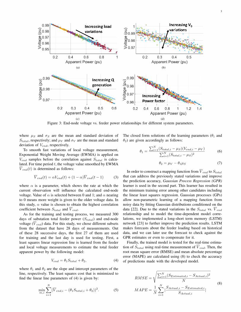
i . This simplification is based on avalid assumption and commonly known as LinDistFlow in theliterature [21]. It significantly reduces the computation timeto solve a distribution system model enjoying this linearity,and hence allows the development of faster algorithms. Fig. 2shows this relationship between an end-node voltage (Vend)and total feeder power (Stotal) in a custom radial distributiongrid. As seen, the relationship remains fairly linear over theoperating voltage range. This suggests that a linear functioncan be built to map these variables using the linear leastsquares estimation. This will be performed in the first partof this study. However, power grid specific dynamics (e.g.,on-load tap changers (LTC) and voltage regulators (VR), capbanks, reactive power injections, node loading variations, andfeeder voltage variations) might introduce noisy non-linearcharacteristics or curve shifts as illustrated in Fig. 3. Theseplots were obtained in a custom-sized distribution grid by vary-ing the system parameters, i.e., by increasing load variations,substation voltage variation (V0), reactive power generation,and power factor. In order to capture these variations anddevelop more generalized models for the relationship betweenVend and Stotal, we will also use more advanced machinelearning regression methods such as GPR and LSTM. Thiswill be performed in the second part of this study.

III. METHODOLOGY

In the proposed framework, the end-nodes will make load-ing decisions by inferring the distribution grid’s congestionlevel from the local voltage Vend they observe. In order toverify that the local voltage measurements can capture thedistribution grid’s congestion level, a correlation study is re-quired to look for relations (correlations) between two randomvariables: (1) Stotal and (2) Vend. Correlation coefficient ofStotal and Vend is a measure of their linear dependence.This dependency and high correlation allow us to constructa mapping from one variable to the other. If each variable hasN scalar observations, then the Pearson correlation coefficientis defined as:

R(Stotal, Vend)=1

N−1

N∑i=1

(Stotal,i−µS

σS

)(Vend,i−µV

σV

)(2)

3

(a) (b)

(c) (d)Figure 3: End-node voltage vs. feeder power relationships for different system parameters.

where µS and σS are the mean and standard deviation ofStotal, respectively; and µV and σV are the mean and standarddeviation of Vend, respectively.

To smooth fast variations of local voltage measurement,Exponential Weight Moving Average (EWMA) is applied onVend samples before the correlation against Stotal is calcu-lated. For time period t, the voltage value smoothed by EWMAV end(t) is determined as follows:

V end(t) = αVend(t) + (1− α)V end(t− 1) (3)

where α is a parameter, which shows the rate at which thecurrent observation will influence the calculated end-nodevoltage. Value of α is selected between 0 and 1; and α nearingto 0 means more weight is given to the older voltage data. Inthis study, α value is chosen to obtain the highest correlationcoefficient between Stotal and V end.

As for the training and testing process, we measured 300days of substation total feeder power (Stotal) and end-nodevoltage (V end) data. For this study, we chose different subsetsfrom the dataset that have 28 days of measurements. Outof these 28 successive days, the first 27 of them are usedfor training and the last day is used for testing. First, aleast squares linear regression line is learned from the feederand local voltage measurements to estimate the total feederapparent power by the following model:

Vend = θ1Stotal + θ2, (4)

where θ1 and θ2 are the slope and intercept parameters of theline, respectively. The least squares cost that is minimized tofind the linear line parameters of (4) is given by:

minm,c

N∑i=1

(V end,i − (θ1Stotal,i + θ2))2. (5)

The closed form solutions of the learning parameters (θ1 andθ2) are given accordingly as follows:

θ1 =

∑Ni=1(Stotal,i − µS)(Vend,i − µV )∑N

i=1(Stotal,i − µS)2(6)

θ2 = µV − θ1µS (7)

In order to construct a mapping function from V end to Stotal

that can address the previously stated variations and improvethe prediction accuracy, Gaussian Process Regression (GPR)learner is used in the second part. This learner has resulted inthe minimum training error among other candidates includingthe linear least squares regression. Gaussian processes (GPs)allow non-parametric learning of a mapping function fromnoisy data by fitting Gaussian distributions conditioned on thedata [22]. Due to the stated variations in the Stotal vs. V end

relationship and to model the time-dependent model corre-lations, we implemented a long-short term memory (LSTM)network [23] to further improve the prediction results. LSTMmakes forecasts about the feeder loading based on historicaldata, and we can later use the forecast to check against theGPR estimates or even to compensate for it.

Finally, the trained model is tested for the real-time estima-tion of Stotal using real-time measurement of V end. Then, theroot mean square error (RMSE) and mean absolute percentageerror (MAPE) are calculated using (8) to check the accuracyof predictions made with the developed model.

RMSE =

√∑Ni=1(SEstimated,i − SActual,i)2

N

MAPE =1

N

N∑i=1

|SActual,i − SEstimated,i

SActual,i|

(8)

4

IV. SYSTEM DESCRIPTION AND EXPERIMENTAL DATA

A. System Description

In this study, a residential feeder located in Alabama isused to analyze the distribution system congestion. This feederis serving approximately 2,000 customers through a radialline. There are four capacitor banks on the feeder rated at1,200 kVAR, 900 kVAR, and two 600 kVARs. One of the600 kVAR capacitors is located at the downstream of the housewe are monitoring. There is also a 10% voltage regulator in thefeeder connected at the upstream of the house in consideration.The transformer of the feeder is a load-tap changer. The feedertotal apparent power data (Stotal) is measured at every 15-minute interval. An eGauge smart meter [24] is installed tothe house located at the downstream of the feeder, whichmeasures one second resolution voltage (Vend) at the houseend. The smart meter records data, and sends it to the cloudusing local Wi-Fi connection. The end-node voltage data ispublicly available at the University of Alabama institutionalrepository [25]. The data is collected in 2019 and 2020 forabout a year. The substation data that powers the householdis provided by Alabama Power which is operated by SouthernCompany.

B. Dataset Generation and Pre-processing

Feeder apparent power data (Stotal) is recorded at 15-minute intervals, whereas the local voltage (Vend) is measuredat one-second resolution. Therefore, 15×24=96 samples ofStotal data and 60×60×24=86,400 samples of Vend data areavailable per day. To equalize the number of samples, a down-sampling operation is applied on Vend data.

The average of 60×15=900 samples is discretely calcu-lated for each 15-minute interval in the Vend data. The dataprocessing is depicted on Fig. 4a. EWMA is applied on thedown-sampled Vend data to remove local dynamic and fastfluctuations (Fig. 4b). EWMA does not affect the sample size,but performs a filtering action on Vend data. For different αvalues ranging from 0.01 to 1.0 with 0.01 increments, V end(t)is calculated according to (3). Then, the correlation coefficientbetween Stotal and V end is computed for each α value. Theoptimum α value is calculated as 0.07 where the maximumcorrelation co-efficient is observed.

V. MACHINE LEARNING MODELS

To understand how closely Stotal and V end data in a scatterplot fall along a straight line, a correlation study is performed.Correlation coefficient (R) measures the strength and directionof a linear relationship. The absolute value of R close to onemeans the data are described better by a linear equation. Datasets with values of R close to zero show little to no straight-line relationship. R for five weekdays of July 2019 is foundas follows: July 15th = −0.8227, July 16th = −0.9870, July17th = −0.9479, July 18th = −0.9765, and July 19th =−0.9842. In all cases, the absolute values of R are greaterthan 0.8. It clearly indicates that Stotal and V end data arealigned and well correlated on a straight line in the scatterplot.

(a)

(b)

Figure 4: (a) Data wrangling for power and voltage data and(b) EWMA applied on local Vend and substation power.

Figure 5: Linear relationship between end node voltage andtotal feeder power for 16 days of July 2019.

5

(a) (b)

(c) (d)

Figure 6: End-node voltage vs. feeder power for four days: (a) July-16, (b) July-19, (c) July-28, and (d) July-29 with each daysplit into four time intervals (colored).

To see the relationship between Stotal and Vend, an X/Y(scatter) plot is used with Stotal along the horizontal axis andVend on the vertical axis. Fig. 5 is constructed with Stotal

and pre-processed Vend data collected from the feeder andthe eGauge meter respectively. The experimental data alsoindicates the quasi-linear relation shown mathematically inSection II. Hence, we model the relationship between Stotal

and Vend linearly, i.e., Vend = θ1 ·Stotal+θ2 where (θ1, θ2) aremodel parameters to be learned. To define their relationship,a line equation is constructed. For instance, the parameters ofthe linear line fit to the data collected over a total of 16 days ofJuly 2019 are estimated as θ1 = −0.5839 and θ2 = 248.2281(Fig. 5).

The insights from analyses and empirical results suggestusing a linear model using LR. We will first investigate theperformance of this model and present the results of LR.However, as previously stated, this linear relationship mightbe exposed to noise, shift, or some other disturbances dueto various dynamics taking place in the grid. Different timesof the day might also have different regulations and thusexhibit different trends. To illustrate this, four July 2019 days(July 16-19-28-29) were split into four time intervals (12AM-6AM, 6AM-12PM, 12PM-6PM, 6PM-12AM), and their end-node voltages are plotted against the corresponding day’s totalfeeder power and shown in Fig. 6. We can clearly see thatthe parameters of the linear relationship are fairly constanton some days (Fig. 6a and Fig. 6b) whereas they are slightlychanged on other days (Fig. 6c and Fig. 6d) especially during6PM-12AM (purple). It can also be seen that different time

frames in a single day have different quasi-linear relations.To that end, GPR and LSTM models will be tested againstclassical LR to improve the prediction performance and theresults will be compared.

To demonstrate how accurately the proposed models canpredict the total feeder power consumption using local end-node voltage measurements, we put them to a test usingfour different days (i.e. Aug. 10 2019, Sept. 8 2019, Jan. 72020, and Apr. 17 2020). We trained the ML models usingMATLAB’s Regression Learner Toolbox. This toolbox hasoptimized hyper-parameters settings to automate the selectionof hyper-parameter values. To protect against overfitting, weused cross-validation by partitioning the dataset into five folds.For time series forecasting, we used an LSTM layer with200 hidden units and trained the model using MATLAB’strainNetwork function.

An important observation is that due to variations in systemmodel parameters (as explained in Fig. 3) for different daysand for different time frames within a day, the system mod-elling should understand such changes for better estimationaccuracy. As an effort towards addressing this, we includedthe day of the week and time of the day information, whichare introduced as two new input features into the learningalgorithm. After these updates, the dataset has three inputs(voltage, time interval, and day of week) and one output(feeder power) for each data sample.

Fig. 7 shows the three estimates, i.e., LR, GPR, and LSTM,for the actual total feeder power. The corresponding end-nodevoltage is also provided on the same plots. The correspondingestimation errors are calculated in terms of RMSE and MAPE

6

(a) (b)

(c) (d)

Figure 7: Actual and estimated total feeder power consumption using LR, GPR and LSTM, and end-node voltage for (a) Aug.10th of 2019, (b) Sept. 8th of 2019, (c) Jan. 7th of 2020, and (d) April 17th of 2020.

(i.e. (8)) and provided in Table I (best results are shown inbold). The correlation coefficients between the actual powervs. end-node voltage (Corr(S, V)) and the actual power vs. theestimated values (Corr(S, LR), Corr(S, GPR), Corr(S, LSTM))are also computed and presented in Table II (best results areshown in bold). The explanation on Fig. 7 and Tables I andII are provided below.

Fig. 7 first shows that LR predictions are able to followthe trends in the total feeder power just by monitoring thelocal voltage as suggested earlier in the paper. Therefore, theperformance of LR is acceptable to some extent but thereis room for development for better prediction accuracy viautilizing GPR and LSTM. For instance, Table I uncovers thatLR estimate errors are higher than that of GPR (except forApril 17th). Although regression can be quite successful inconstructing a mapping function to predict the total powerusing end-node voltage and other features (time interval andday of week), it is still prone to errors, i.e., the learnedrelationship becomes highly invalid/violated for the day ofprediction. We see such a problem with the GPR estimateespecially on 17th of April. To deal with this problem, wealso implemented an LSTM network to make a prediction onthe next day’s total power by providing the previous days’data. This can serve as a guidance for the final prediction andhelp us check the accuracy of GPR.

Both estimations (GPR and LSTM) for Aug. 10th (Fig. 7a)and Sept. 8th (Fig. 7b) closely follow the actual value thoughthey are slightly off especially after 5PM. Table I shows thatGPR made better estimates compared to LSTM, suggestingthat the final prediction should be closer to that of GPR for

Table I: RMSE and MAPE scores for LR, GPR, LSTMestimations.

Days RMSE(LR)

RMSE(GPR)

RMSE(LSTM)

MAPE(LR)

MAPE(GPR)

MAPE(LSTM)

Aug. 10, 2019 0.4154 0.3866 0.4916 0.0613 0.0575 0.0716Sept. 8, 2019 0.7573 0.5954 1.0040 0.1051 0.0740 0.1271Jan. 7, 2020 0.5731 0.3420 0.7023 0.0840 0.0771 0.1075Apr. 17, 2020 0.3703 0.5758 0.1826 0.0812 0.1277 0.0366

Table II: Correlation scores between actual power vs. actualvoltage, LR, GPR, and LSTM estimations.

Days Corr (S, V) Corr(S, LR) Corr(S, GPR) Corr(S, LSTM)Aug. 10, 2019 -0.9690 0.9690 0.9761 0.9762Sept. 8, 2019 -0.9770 0.9770 0.9622 0.9691Jan. 7, 2020 -0.9174 0.9174 0.9368 0.8587Apr. 17, 2020 -0.6745 0.6269 0.5807 0.9074

these two days. Fig. 7c and Fig. 7d demonstrate the resultsfor Jan. 7th and Apr. 17th. We see double peaks in the totalpower consumption since the data belongs to different seasonsof the year. On Jan. 7th, the LSTM estimate stays below theactual consumption, however, this can be compensated by theGPR estimate since its error values are much smaller (Table I).Interestingly, the LSTM estimate between 12PM-6PM is moreaccurate than that of the GPR estimate. This suggests that thefinal estimate could be weighted more towards LSTM duringthis time interval. On Apr. 17th, we see the GPR estimate isfar off the actual consumption even though it can still detectthe trends (peaks) in the consumption via voltage mapping.This is because the GPR estimation is based on the measuredlocal voltage and the voltage of this day is poorly correlatedwith the actual power resulting in a correlation coefficient of-0.6745 (Table II). However, the LSTM estimate gives a much

7

more accurate prediction resulting in the lowest RMSE valueamong all testing results. For this day, the compensation for thefinal prediction should be weighted more towards the LSTMestimate.

VI. CONCLUSIONS AND FUTURE WORK

This study investigates how loading of grid assets, such assubstation transformers and feeders, can be mapped to localvoltage, and how this mapping can be used to locally estimatethe network congestion level in real time. Correlation studyrevealed that the relationship between the feeder power andthe local voltage is highly linear, and thus can be formulatedby a linear function using LR. It has been showed that thedegree of correlation can be increased with EWMA by filteringout the noises present in the local voltage data. To validatethe approach, the study estimated the real-time feeder powerof a real substation in Alabama by using the real-time end-node voltage, day, and time information using RL, GPR,and LSTM. The results showed that the estimations closelyfollow the actual value for the testing days (the best RMSEsranging from 0.1826 to 0.5954). However, we also observedthat the estimates seem off from the actual power consumptionfor some days. This suggests the presence of other voltageregulation actions taking place at the upstream/downstreamnetwork that can cause violation in the derived mappingfunction and result in low accuracy. In those cases, the bestestimate can be obtained using a weighted combination ofestimates (such as GPR and LSTM) since one may performbetter than the other for a particular day compensating theerror. Therefore, our future study will involve how to combinethe results of both estimates to make more accurate unifiedpredictions of critical feeder operation points for the purposeof enhancing and improving the grid operation.

ACKNOWLEDGEMENT

The authors would like to thank Brooke Williams, TomCanada, Derl Rhoades, and Andrew Ingram from SouthernCompany for their help and support in accessing the substationfeeder data, and for thoughtful discussions.

REFERENCES

[1] (2015) Study: Electric vehicles can dramatically re-duce carbon pollution from transportation, and improveair quality. https://www.nrdc.org/experts/luke-tonachel/study-electric-vehicles-can-dramatically-reduce-carbon-pollution.[Online; accessed 10-Jan-2020].

[2] F. Erden, M. C. Kisacikoglu, and O. H. Gurec, “Examination of EV-grid integration using real driving and transformer loading data,” in Int.Conf. Elect. Electron. Eng., 2015, pp. 364–368.

[3] L. P. Fernandez, T. G. S. Roman, R. Cossent, C. M. Domingo, andP. Frias, “Assessment of the impact of plug-in electric vehicles ondistribution networks,” IEEE Trans. Power Syst., vol. 26, no. 1, pp. 206–213, Feb. 2011.

[4] S. Shafiee, M. Fotuhi-Firuzabad, and M. Rastegar, “Investigating the im-pacts of plug-in hybrid electric vehicles on power distribution systems,”IEEE Trans. Smart Grid, vol. 4, no. 3, pp. 1351–1360, 2013.

[5] E. Veldman and R. A. Verzijlbergh, “Distribution grid impacts of smartelectric vehicle charging from different perspectives,” IEEE Trans. SmartGrid, vol. 6, no. 1, pp. 333–342, 2015.

[6] N. Leemput, F. Geth, J. Van Roy, A. Delnooz, J. Buscher, and J. Driesen,“Impact of electric vehicle on-board single-phase charging strategies ona flemish residential grid,” IEEE Trans. Smart Grid, vol. 5, no. 4, pp.1815–1822, 2014.

[7] K. Clement-Nyns, E. Haesen, and J. Driesen, “The impact of chargingplug-in hybrid electric vehicles on a residential distribution grid,” IEEETrans. Power Syst., vol. 25, no. 1, pp. 371–380, Feb. 2010.

[8] S. Huang, Q. Wu, L. Cheng, and Z. Liu, “Optimal reconfiguration-baseddynamic tariff for congestion management and line loss reduction indistribution networks,” IEEE Trans. Smart Grid, vol. 7, no. 3, pp. 1295–1303, May 2016.

[9] O. Sundstrom and C. Binding, “Flexible charging optimization forelectric vehicles considering distribution grid constraints,” IEEE Trans.Smart Grid, vol. 3, no. 1, pp. 26–37, Mar. 2012.

[10] J. Hu, S. You, M. Lind, and J. Østergaard, “Coordinated charging ofelectric vehicles for congestion prevention in the distribution grid,” IEEETrans. Smart Grid, vol. 5, no. 2, pp. 703–711, Mar. 2014.

[11] T. Ganu, J. Hazra, D. P. Seetharam, S. A. Husain, V. Arya, L. C. DeSilva, R. Kunnath, and S. Kalyanaraman, “nplug: A smart plug foralleviating peak loads,” in Int. Conf. on Future Syst., May. 2012.

[12] T. Ganu, D. P. Seetharam, V. Arya, J. Hazra, D. Sinha, R. Kunnath,L. C. D. Silva, S. A. Husain, and S. Kalyanaraman, “nplug: Anautonomous peak load controller,” IEEE J. Sel. Areas Commun., vol. 31,no. 7, pp. 1205–1218, July 2013.

[13] L. Xia, T. Alpcan, I. Mareels, M. Brazil, J. de Hoog, and D. A. Thomas,“Modeling voltage-demand relationship on power distribution grid fordistributed demand management,” in Australian Control Conf. (AUCC),Nov. 2015.

[14] L. Xia, T. Alpcan, I. Mareels, M.Brazil, J. de Hoog, and D. A. Thomas,“Local measurements and virtual pricing signals for residential demandside management,” Sustain. Energy, Grids and Netw., Dec. 2015.

[15] L. Xia, J. de Hoog, T. Alpcan, M. Brazil, I. Mareels, and D. Thomas,“Electric vehicle charging: A noncooperative game using local measure-ments,” IFAC Proc. Volumes, vol. 47, no. 3, pp. 5426–5431, 2014.

[16] F. Geth, N. Leemput, J. Van Roy, J. Buscher, R. Ponnette, and J. Driesen,“Voltage droop charging of electric vehicles in a residential distributionfeeder,” in IEEE PES ISGT Europe, Oct. 2012, pp. 1–8.

[17] P. Richardson, D. Flynn, and A. Keane, “Optimal charging of electricvehicles in low-voltage distribution systems,” in IEEE Power EnergySoc. General Meeting, July 2012.

[18] E. Ucer, M. C. Kisacikoglu, and A. C. Gurbuz, “Learning EV integrationimpact on a low voltage distribution grid,” in IEEE Power Energy Soc.General Meeting, Aug. 2018, pp. 1–5.

[19] E. Ucer, M. C. Kisacikoglu, M. Yuksel, and A. C. Gurbuz, “An internet-inspired proportional fair EV charging control method,” IEEE Syst. J.,vol. 13, no. 4, pp. 4292–4302, Dec. 2019.

[20] E. Ucer, M. C. Kisacikoglu, and M.Yuksel, “Analysis of decentralizedAIMD-based EV charging control,” in IEEE Power Energy Soc. GeneralMeeting, Aug 2019, pp. 1–5.

[21] M. Baran and F. F. Wu, “Optimal sizing of capacitors placed on a radialdistribution system,” IEEE Trans. Power Del., vol. 4, no. 1, pp. 735–743,1989.

[22] M. F. Huber, “Recursive gaussian process regression,” in IEEE Int. Conf.Acoustics, Speech Signal Process., 2013, pp. 3362–3366.

[23] S. Hochreiter and J. Schmidhuber, “Long short-term memory,” NeuralComput., vol. 9, no. 8, p. 1735–1780, Nov. 1997.

[24] Energy monitoring systems for residential and commercial applications.http://www.egauge.net/. [Online; accessed 31-Jan-2018].

[25] E. Ucer, S. Rahman, A. McDonald, and M. Kisacikoglu. (2019) Residen-tial active/reactive power consumption, voltage, and frequency data fora house in Alabama. [Dataset] https://ir.ua.edu/handle/123456789/6346.[Online; accessed 15-Jul-2020].