720 IEEE TRANSACTIONS ON POWER SYSTEMS, VOL. 5 , NO. 3, AUGUST 1990

A Low-Order System Frequency Response Model

P. M. Anderson, Fellow, IEEE M. Mirheydar, Member, IEEE Power Math Associates, Inc.

Del Mar. California

Abstract This tutorial paper presents the derivation of a simple, low order System Frequency Response (SFR) model that can be used for estimating the frequency behavior of a large power system, o r islanded portion thereof, t o sudden load disturbances. The SFR model is a simplification of other models used for this purpose, but it is believed to include the essential system dynamics.

The SFR model is based on neglecting nonlinearities and all but the largest time constants in the equations of the generating units of the power system, with the added assumption that the generation is dominated by reheat steam turbine generators. This means that the generating unit inertia and reheat time constants predominate the system average frequency response. Moreover, since only two time constants predominate, the resulting system response can be computed in closed form, thereby providing a simple, but fairly accurate, method of estimating the essential characteristics of the system frequency response.

Keywords Frequency, islanded operation, uniform frequency, reheat time constant, governor droop, regulation, inertia constant, damping, load-frequency behavior, frequency rate of change, frequency response.

Introduction Frequency response models have received limited treatment in the literature. The basic concept of the model derived here is based on the idea of uniform or average frequency, where synchronizing oscillations between generators are filtered out, but the average frequency behavior is retained. The synchronizing oscillations are illustrated in Figure 1, taken from the Florida simulations of reference [l]. We seek to average these individual machine responses with a smooth curve that can be used t o represent the average frequency for the system. Such a filtered or average frequency is shown by the heavy line in Figure 1.

The concept of a uniform frequency model has been explored by numerous investigators dating back 50 years or more. Our approach is similar t o that of Rudenberg [21, who provides many references on the subject as well as a mathematical derivation of the basic concept. Similar and related approaches have been pursued more recently [3,4] through work on energy functions. The basic ideas are also important in the work on system area control simulators [5,6], as well as the work on long

90 5.: 006-7 P !I paper recoiinen$.ed an$. by t i l the I a t th a'ebruary 4 - 8, 1390. i .anuscr ipt submitter1 August 22, 1389: node a v a i l s b l e f o r p r i n t i n : Decmber 27, 19S9.

?over Systc :? Ii igineerin;; Commit !er dng inee r ing Soc ie ty for p r e s e n t a t i o n PiCS 1990 ' l i n t e r i k e t i n z , !,,flnnta, Ceor :iii,

58 8 4 4

0 1 2 3 4 5 nrne In seconds

Figure 1 Simulated Unit Frequencies and System Average Frequency After Islanding

term dynamics [7,8]. In addition to these resources, certain ideas have also been adopted from the work on coherency based dynamic equivalents [9,10], as well as the work on transient energy stability analysis [ll]. A related, but quite different approach, has been taken by in the work on emergency control [12], but this model is more complex than believed necessary and is more difficult to use than the method presented here. The analysis and results found here are similar t o that of references 13 and 14, but our model is simpler. References 15-17 provide still other methods of analyzing the problem of frequency behavior, in varying degrees of complexity. Our approach is to provide the minimum order model that retains the essential average frequency response shape of a system with typical time constants and active speed governing.

The basic SFR model averages the machine dynamic behavior in a large system into an equivalent single machine. Topologically, we can think of the separate machines being replaced by a single large machine that is connected t o the individual generator buses through ideal phase shifters. The result is a representation of only the average system dynamics, while ignoring the intermachine oscillations shown in Figure 1. There are theories that can be used t o determine the total impedance to a so-called "inertial center" [3,4,18], but it is probably adequate to consider only the generator and transformer impedances.

The effect of these impedances places a limitation on the amount of load that any generating unit can absorb [19- 201. Our model neglects this limitation, although we acknowledge the validity of the concept. We assume here that the disturbance is small compared to the total rating of the island, and that the equivalent machine will be able to absorb this change. The model can be easily adapted, however, t o limit the load change.

TheSFRModel Consider a large system in which most of the generating units are reheat steam turbine units. We wish t o reduce this system t o one described by a minimum number of equations that will compute only the average frequency behavior. In this system, the dynamic performance of

0885-8950/90/08OO-0720$01 .OO 0 1990 IEEE

1

I

each rotating mass is controlled by a separate governor by integrating the individual accelerating power.

$.

t I Boiler

Boiler Ref

Figure 2 Generating Unit Frequency Controls

A general diagram of an individual power plant is shown in Figure 2. The SFR model examines only the midrange frequencies associated with changes in shaft speed. For this purpose, we may ignore the thermal system dynamics of the boiler as being too slow, and also the generator response as being too fast. This leaves a reduced system consisting of the governor servo motors, steam turbine, and inertia. A typical illustration of a typical governor-turbine model is shown in Figure 3 [21].

1 LE"" I I

Figure 3 Typical Reheat Turbine Governor Model

The most significant time constant in this system is the reheater time constant, identified as T R in Figure 3. This constant is usually in the range of about 6 to 12 seconds and tends to dominate the response of the largest fraction of turbine power output. Therefore, we ignore all the smaller time constants as insignificant compared to T . The second dominant time constant in the system is &e inertia constant, called H in Figure 2, This constant is on the order of 3 t o 6 seconds for a typical large unit and is always multiplied by two, which increases its effect. The third dominant constant is the 1lR constant, the inverse of the governor regulation, which acts as a gain in the control diagram.

If we assume that the two time constants for the reheat and inertia dominate the response in the first few seconds, we have the reduced plant model to that shown in Figure 4.

We identify the following quantities in Figure 4:

P, = Incremental power set point, per unit P, = Turbine mechanical power, per unit

Pa = P, - P, = Accelerating power, per unit Am = Incremental speed, per unit FH = Fraction of total power generated by the HP turbine TR = Reheat time constant, seconds H = Inertia constant, seconds D = Damping Factor

= Generator electrical load power, per unit

K,,, = Mechanical Power Gain Factor

72 1

I I I I

Figure 4 The Reduced Order SFR Model

By direct block diagram analysis of Figure 4, we compute

(2)

2HR+(DR+ K,FH)TR ' = [ 2(DR+ K,)

Obviously, from ( l ) , the nature of the response to a change in either P or P, is of the same form, but of different sign and p%',se.

In the many studies, we are interested only in a change in P (with Psp = 0). For this problem, characterized by a sudden load upset, we can further simplify the system to that shown in Figure 5, where we define a "disturbance power" Pd as the new system input variable. Here we have chosen the sign of Pd such that

Pd > 0 For a sudden increase in generation

Pd < 0 For a sudden increase in load (3)

- T - 1

I I Figure 5 Simplified SFR Model with Disturbance Input

For this, the special problem of interest, we compute the frequency response in per unit to be

I ( Rmi 1 ( l + T R s ) p d A@= - DR + K , s2 + 2 p n s + 61; (4)

and the per unit speed or frequency can be computed for =YPd

For sudden disturbances we are usually interested in Pd in the form of a step function, i.e.,

P,(t) = p s f . p u(t) (5)

122

where P,, is the disturbance magnitude in per unit based on tfie system voltampere base SsB and u(t) is the unit step function. In the Laplace domam, we write

PJS) = (6)

and this expression can be substituted into (4) with the result

This equation can be solved directly to write, in the time domain,

. . where

a=,/- 1 - 2T SW, +T'W: 1- s"

W, = W , d l - S Z and

The time response (8) is a damped sinusoidal frequency deviation, expressed in per unit.

Normalization The equations shown above are typical of any reheat unit in the system, with all equations assumed to be in per unit on some base. Let us asgume that all are in per unit on a common system base, S,. We now combine all units into a single large unit that represents all generating units in the entire system. This can be done by adding the power equations, as follows:

c 2 H i s A ~ = c P , - c P , I I I (11)

(1 2)

(1 3)

where we assume that all equations are on a common system base S,. We now renormalize (11) to (13) to the total system base S,, which is equal to the s u m of the ratings of all generating units in the system.

n

SsB = CSBi i=l (14)

This change of base multiplies (11-13) by the ratio of the two bases with the result

(1 5)

which defines the equivalent generator parameters. The normalized value of these parameters on the total system base will be typical of those for a single unit on its own base.

The parameter K is an effective gain constant that expresses the t o d f mechanical power in terms of the governing valve area. This gain is affected by the system power factor and by the spinning reserve, as follows.

where Fp = Power Factor fsR = Fraction of Units on Spinning Reserve

We assume a constant power factor for all units.

Example As an example of the computation of the SFR consider a system with the following typical parameters.

R = 0.05 H = 4 . 0 s K,,, = 0.95 FH = 0.3 TR=8.0s D = 1.0

Then we compute

W, = 0.559 go,, = 0.438 $1 = 131.94' g = 0.783 W, = 0.348 q2 = 141.54'

a = 6.011 41 - 52 = 0.622 I$ = -9.60'

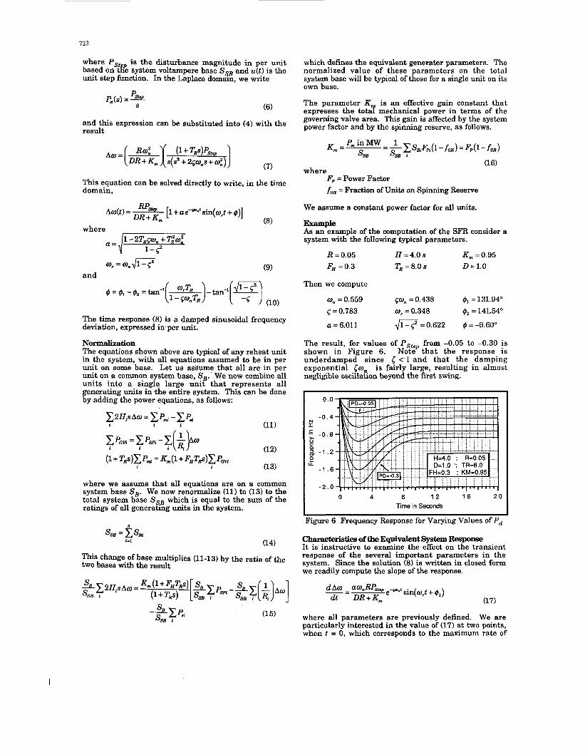
The result, for values of Pstep from -0.05 to -0.30 is shown in Figure 6. Note that the response is underdamped since < 1 and that the damping exponential run. is fairly large, resulting in almost negligible oscillation beyond the first swing.

0.0

- 0 . 4

-0.8 I

0

g -1.2 s! U

- 1 .6

-2.0 0 4 8 12 16 20

Time in Seconds

Figure 6 Frequency Response for Varying Values of Pd

CharacteristiaoftheEquivalentSystemResponse It is instructive to examine the effect on the transient response of the several important parameters in the system. Since the solution (8) is written in closed form we readily compute the slope of the response.

(1 7)

where all parameters are previously defined. We are particularly interested in the value of (17) at two points, when t = 0, which corresponds to the maximum rate of

1

723

change of slope, and when the slope is zero, which corresponds to the maximum frequency deviation.

1. t=O

dw dt

2. -=o

Equation (19) is satisfied when wrt + integer, including zero. compute

= na for n an If we call this time t,, we

(20)

These slope parameters are clearly observed in Figure 6. The initial slope depends only on P and H, hence it changes for each run plotted in the f$&re. However, t, is not a function of PSte , so the maximum frequency deviation occurs at exacdy the same time (2.35 s) for all disturbances. Note also that Figure 6 is plotted in hertz so all equations must have been multiplied by 60.

Another parameter that can be readily checked is the regulation. Governors are set with droop R to give a steady-state speed vs. power relationship of

RP,, Am = DR + K , (21 1

where both w and P,,, are incremental, normalized quantities. Note that f i p p must take the sign of P, , which would be negative or an increase in load or loss of generation. Thus, in Figure 6, where we let Pstep = -0.3 and R = 0.05 we compute

which is clearly observed in Figure 6. This result can be also be verified mathematically by the final value theorem

limAw(t) = ; p A w ( s ) = RpSkp

(22) t+- DR + K,,,

I t is difficult to visualize the effect of each physical parameter of the SFR model without plotting the results. Therefore, each parameter is now varied in turn and the results plotted to illustrate the effect of that parameter.

The E€Fectof Governor Dmop,R The value of R is varied from 0.05 to 0.10 in increments of 0.01 per unit. The results are shown in Figure 7. Actual observed system responses in islanded situations have sometimes shown the net system regulation to be in the neighborhood of 0.1.

This indicates that some generating units are operating with governor valves blocked, giving a regulation of 1.0 per unit for these units. This increases the net regulation for the system in proportion to the size of the units with blocked valves. Note in Figure 7 that the steady state regulation is exactly as given by (21). Thus,

0.0

- 0 . 5 2 .c - 1 . 0 $ ?5 2 - 1 . 5

-2.0

- 2 . 5

LL

0 4 8 1 2 1 6 2 0 Time in Seconds

Figure 7 Frequency Response for Varying Values of R

for the disturbance with Pstep = - 0.2 and DR + K =1, as illustrated, we compute Aw = 60 (0.2) R = 12 R &r each case. The simulation shown in Figure 7 must be extended for a rather long time to accurately observe the final value. It is also important to note that the assumed droop setting R has absolutely no effect on the initial rate of frequency decline. This is important. Even if all governors are a t the extreme valve-closing end of their individual backlash limits, as in following a gradual load decrease, a sudden loss of load would require a rapid change to a valve open condition. While traversing this backlash region, the system is operating essentially open loop and the natural 100% turbine regulation prevails. However, the initial rate of change is the same as for a tightly tuned system with no backlash. This effect can be noted in Figure 5, where the regulation term is seen to be affected by the lag of the feedback term, which is a "lag-lead'' function. The difference regulation makes is in the recovery time, the maximum offset, and the final value. It is important that this recovery be fast in order to limit the time of exposure at frequencies below about 58 Hz.

I I I I I I I

0 0.1 0.2 0.3 0.4 Disturbance Magnitude in per unit

?igure 8 Max Frequency Deviation vs. Disturbance Size

The value of R is probably bounded hetween about 0.05 and 0.10 for most systems. This effectively bounds the maximum frequency deviation for a given disturbance to the shaded region shown in Figure 8. Here, the disturbance is the step function magnitude, as before. Figure 8 is plotted with nominal values of the other parameters (H = 4.0 s, T = 8.0 s, FH = 0.3, K,,, = 0.95, D = 1.0). The maximum Sisturbance power is actually limited, as discussed in 1201, but this is not considered in the calculation of values for Figure 8.

I ' --

124

The EfEect of Inertia, H The value of H has a direct effect on the initial slope, as shown in the simulations of Figure 9 for various H values. I i

0.0

-0.2

9 -0.4 c .- x - 0 . 6

2 -0.8 f

E -1.0 -1.2

-1.4 0 4 8 12 16 2 0

Time in Seconds

Figure 9 Frequency Response for Varying Values of H

The inertia constant affects almost all response measures, including on, and <, as given by equation (21, and thereby all other computed parameters as given by, (9) and (lo), including the initial slope and the time t, of maximum frequency deviation as given by (18) and (191, respectively. It is also interesting to observe that (1/2H) is the forward loop gain in Figure 5. Note also that H is involved only in the forward loop. All other parameters are feedback parameters.

The most pronounced effect of changes in H is the change in the initial slope, and the time of the peak response. Note that H does not affect‘the final steady- state value of frequency.

The Effect of Reheat Time Constant, TR The reheat time constant is an important system parameter. Usually 70% or more of the turbine output is delayed by the reheat time constant and the variation of this time lag has a pronounced effect on frequency performance. Figure 10 shows a range that is typical of large generating units. T has an effect on the damping ratio c and the natural unjamped frequency U,, but does not effect the initial slope or the final value.

0.0

-0.2

2 -0.4 z1 -0.6

J -0.8

- 1 . 0

-1.2

- 1 . 4

K .- c

0 4 8 12 16 20 Time in Seconds

Figure 10 Frequency Response for Varying Values of TR

TheEffectofHighFkssureF’raction,FH The constant F measures the fraction of shaft power developed by t fe high pressure turbine on a single reheat system. This is the fraction of shaft power that is not delayed by reheating. Figure 11 shows the effect of varying only FH, with other parameters at their nominal

values. Large values of FH, have a pronounced effect on c and can make the system overdamped ( c > 1). When this occurs, the frequency response is not given by (8), but is a combination of exponentials. The frequency response equation for this condition is computed from (7) by factoring the quadratic t o write

Then

In the numerical example plotted in Figure 11, when FH, is greater than 0.4, the system is overdamped. This corresponds to the three curves with the smallest frequency displacement in the figure.

0.0 -0.2

3 -0.4 -‘ - 0 . 6 X

-0.8 3 p - 1 . 0 l i -1.2

-1.4

0 4 8 12 16 2 0 Time in Seconds

Figure 11 Frequency Response for Varying Values of FH

Performance Analysis and Model Restrictions Performance analysis for a given system using the SFR model is relatively easy, providing data from an actual system disturbance is available to tune the parameters. Actual system disturbance records are necessary since some system parameters are almost impossible t o determine due t o unknown operating conditions. Regulation or droop (R), for example, depends on turbine droop adjustment, the effect of large nuclear units with blocked governor valves, and also the frequency dependence of the load. However, this effect is clearly revealed in the frequency record of an actual disturbance by observing the steady-state frequency error. This steady-state error can be computed from (21) to be

(25)

If the disturbance magnitude is known, and it usually is easily estimated, then R can be estimated. Note that the denominator of (25) is approximately unity in most cases. which helps in making the estimate.

The~ofFrequencyDependenceof~ Power system loads are known to be sensitive t o system frequency. One way of characterizing this dependence is to model the load as having a constant component as well as a frequency dependent component.

PL =PL,(1+k,Aw) (26)

1 -

725 Then the incremental change in load is a function of the incremental change in frequency. But this effect is already included in the model in the form of the damping constant D , where we may write

A€L = DAo (27)

where all values are in per unit. The damping constant is usually used to represent the damping of the load and other effects to rotor oscillations. From Figure 4, however, we note that the product (27) is of the same sign as the electrical power, which is exactly the incremental load of the system. Thus, we have both components of load represented, the constant portion and the frequency dependent portion.

From equations (2) and (81, we see that the system undamped natural frequency and damping are functions of D , but this dependence always appears as the product DR. Since R is small, nominally about 0.05 per unit, the product DR will also be small and the effect of D is diminished. We can illustrate the effect of D on the frequency response by plotting for various values of this parameter, with the results seen in Figure 12. Note the similarities to Figure 7, but with reduced effect.

2 c x c =I

.-

H U

0.0

-0.2

-0.4

-0.6

-0.8

- 1 . o -1.2

-1.4 0 4 8 12 16 20

Time in Seconds

Figure 12 Frequency Response for Various Values of D

Use of the SFR Model F o r b Actual System Disturbance Data for an actual system separation is used to validate the SFR model. The physical system, in this case, separated and islands were created, one with excess generation and one with excess load. The simulation presented is for the island with excess load. The size of the disturbance and steady state frequency error are known and H is easily estimated with confidence. Only the reheat time constant needs to be estimated by trial and error. The result is shown in Figure 13, where the discrete points are the actual system frequency at the point of measurement and the smooth line is the simulation of that frequency.

Note that the data from the physical system includes the effect of the oscillation of local machines with respect to other machines in the island. This is usually the case, and measurements from different parts of the island will show these local oscillations, similar to the machine plots in Figure 1. The local machines oscillate about the average system frequency, which is computed by the SFR model.

CompanisonwithOtherModelsofFrequencyBehavior One application for frequency response models is for the setting of underfrequency load shedding relays, where relays are used to shed portions of the load and thereby restore load-generation balance. One method of

2 0.0 .g -0.2 g -0.4

d - o . 8 p -1.0 8 -1.2 g -1.4

.r( + cr~ -0.6 '5

?

-1.6 0 2 4 6 8 10

Time in Seconds

Figure 13 Model Validation for an Actual Disturbance estimating frequency behavior for this purpose is to model the frequency decline following the disturbance, using a model that reflects the load and generator behavior [21]. This model results in a first order differential equation that has the solution

(28)

This model describes the frequency trajectory as it falls from its initial value in an exponential fashion. The initial rate of decline is as given in (181, but the subsequent rate of decay is faster than that predicted by (17) since the exponential model does not include the governor behavior. Still, this model is often used for determining the time a t which load shedding relays should be employed and is attractive for its simplicity. Note that only the inertia and damping are required to find the frequency for a disturbance of any size. The exponential model (28) includes the effect of load frequency dependence D . As noted before, the D effect is similar to that of governor droop R , but R is much more important in its end result. I g 0.

.B - 0 . g - 1 .

.r( 4 Ld - 1 . '5

h -2.

?

a" -2. 8 -3. g -3. &I

E - 4 .

. o 5 0 5 0

5 0

5 0

0 4 8 12 16 20 Time in Seconds

Figure 14 Comparison of SFR and Exponential Models

Other models described in the references are more complex and will not be described here in detail.

COnclusioas The SFR model of system frequency behavior following an islanding event or a large disturbance on the interconnected system is a greatly simplified model of system behavior. The model developed for this purpose omits many details and ignores small time constants in an effort to provide a model that may be useful in approximating the system frequency performance, including the essential behavior of speed governing and turbine response. However, in spite of the model

126

simplicity, the comparison with actual system disturbances and detailed stability simulations, as shown in Figures 13 and 1 , respectively, are rather encouraging. Moreover, the model provides a n understanding of the way in which important system parameters affect the frequency response. Such understanding is difficult t o achieve in high order models, where performance is a very complex function of many system variables.

1.

2.

3.

4.

5.

G .

7.

8.

9.

10.

11.

12.

13.

14.

Refbrences A. N. Darlington, "Response of Underfrequency Relays on the Peninsular Florida Electric System for coss of Generation," A aper presented at the Georgia Institute of Technofogy Relay Conference, May 4,1978.

Reinhold Rudenberg, Transient Performance of Electric Power Systems; Phenomena in Lumped Networks, MIT Press, Cambridge, MA, 1967.

C. Tavora and 0. J. M. Smith, "Stability Analysis of Power Systems, Report ERL-70-5, College of Engineering, University of California, 1970.

K. N. Stanton, "Dynamic Energy Balance Studies for Simulation of Power Frequency Transients," Proc PICA Conference, IEEE PES, C26-PWR, 1971.

S. Virmani, S. Kim, R. Podmore, T. Athay, and D. Ross, Development and Implementation of Advanced Automatic Generation Control, Final Report of Task 1 , Modeling and Analysis of the WEPCO System," and "App. A, AGC Simulation Program User's Guide," SCI Proj 5215, DOE Contract EC-77-03 -21! 8, P d o Alto, 1979.

Lawrence M. Smith and John H. Spare, "Area Control Simulator Program; v 1 , Technical Manual," EPRI EL-1648, Palo Alto, 1980.

Richard P. Schulz, Anne E. Turner, and Donald N. Ewart, Long Term Power System Dynamics," EPRI Report 90-70-0, Palo Alto, 1974.

Richard P. Schulz and Anne E. Turner,,,"Long Term Power System Dynamics, Phase 11, EPRI EL-367, Pal0 Alto, 1977.

Robert W: deMello, Robin Podmore and K. Neil Stanton, Coherency Based Dynamic Equivalents for Transient Stability Studies," EPRI Report 904, Palo Alto, 1975.

Robin Podmore and Alain Germond, "Development of Dynamic Equivalents for Transient Stability Studies," EPRI EL-456, Palo Alto, 1977.

T. Athay, V. R. Shfrkat, R. Podmore, S. Virmani, and C. Puech, Transient Energy Stability Analysis," SCI Proj 5158, DOE Contract EX-76-C-01- 2076, Palo Alto, 1979.

MIT Staff Report, "Emergency State Control of Slow Speed Dynamics," Final Report, DOE Contract E-49- 18-2075, Cambridge, 1979.

Leon K. Kirchmayer, Economic Control of Interconnected Systems, John Wiley and Sons, New York, 1959.

C. Concordia, F. P. deMello, L. K. Kirchmayer, and R. P. Schulz, "Effect of Prime-Mover Response and Governing Characteristics on System Dynamic Performance, Proc. Am. Power Conf, v XXVIII, 1966, p 10741085.

-

15.

16.

17.

18.

19.

20.

21.

22.

Man L. Chan, R. D. Dunlop and Freed Schweppe, Dynamic Equivalents for Average System

Frequency Behavior Following Ma'or Disturbances," IEEE paper T 72 075-5, presented at the IEEE PES Winter Meeting, New York, Jan/Feb 1972.

D. Crevier and Fred C. Schweppe, "The Use of Laplace Transforms in the Simulation of Power System Frequency Transients," IEEE Trans, v PAS- 94, n 2, MarlApr 1975.

V. N. Manohar and M. K. Sinha, "Choice of Power System Model for Study of Nuclear Plant Dynamics," CIGRE paper 32-12,1976.

P. M. Anderson and A. A. Fouad, Power System Control and Stability, Iowa State University Press, Ames, 1978.

M. S. Baldwin, M. M. Merrian, H. S. Schenkel, and D. J. VandeWalle, "An Evaluation of Loss of Flow Accidents Caused by Power System Frequency Trans ien ts i n Westinghouse PWR's, Westinghouse Report WCAP-8424, May 1975.

M. S. Baldwin and H. S. Schenkel, "Deter+nation of Frequency Decay Rates During Periods of Generation Deficiency," IEEE Trans., v PAS-95, n 1, Jan/F'eb 1976. Stephen R. Lightfoot, Joseph D. Whitaker and Dennis L. Brown, "EPRI Transient-Midterm Stability Program and Plot Program User's Manual," EPRI EL-597, Palo Alto, 1979.

Warren C. New, Ed., "Load Shedding, Load Restoration and Generator Protection Using Solid- State and Electromechanical Underfrequency Relays," General Electric Company Publication GET-6449,1977

Biographies of the Authom P. M. Anderson was born in Iowa and holds the B.S., M.S., and Ph.D. degrees in E.E. from Iowa State University. He has worked for utilities, taught E.E. at two universities, and served as an EPRI research manager. He is currently President and Principal Engineer for Power Math Associates, Inc., a consulting engineering firm in Del Mar California.

Mahmood M irhevdar was born in Iran. He obtained the B.S. and M.S. degrees from the University of Iowa and the Ph.D. degree from Iowa State University, all in Electrical Engineering. He is a Senior Engineer with Power Math Associates, Inc. in Del Mar, California. Dr. Mirheydar specializes in system analysis, modeling, and computer methods for power systems.

727

As the authors state, this paper is a tutorial, in that the model highlights the most important parameters of the power system. It apars to me that the model, if relatively easy and inexpensive to use, can be a screening tool. mere are many perturbations of unit frequencies around the average system frequency, as shown in Figure 1. Studies using more complex models can make definition of the average response difficult to define. m e foregoing statement is not intended to suggest that, in some cases, the local variations from the average response should not be studied, but the use of this model could reduce the number of cases which would have to be studied with a more complex model.

It is stated that all of the generators of an islanded portion of a power system are represented by a single large unit connected to the generator buses through ideal phase shifters. Haw many generator and load buses were represented in the parametric study for which the results are shown in Figures 7 through 12? Were the load buses separate from the generator buses? For Figure 1, how closely did the system represented with the SFR model compare with that used for the simulated unit frequencies?

The parameter K is affected by the system power factor. w a s them power factor used as a variable parameter? If so, what were the results? References 19 and 20 report the results of investigations made to determine maximum frequency decay rates. In follow-up investigations, it was noted that the initial drop in frequency was aggravated by generators operating in the underexcited condition, ie, absorbing reactive power from the system. In this case, the voltage regulator action, shortly after the imposition of the overload, aggravated the frequency decay. ?here is no mention of voltage regulator simulation in the SFR model, although the turbine governor .is represented. It should be noted that present day digital governing systems sample and correct only once or twice a second. Would the authors comment on these points?

Manuscr ip t r e c e i v e d February 20, 1990.

Diseussion

M. E. Connolly, (Houston Lighting & Power Co., Houston, Texas): The authors are to be congratulated on their reduced order model of system frequency response. The matter of system frequency response has been a topic of major interest in the Electric Reliability Council of Texas since the region operates as an island not synchronously connected to the national grids. Various methods for simplified computation of system frequency response to loss of generation disturbances have been investigated.

One general observation that has come out of these investigations is that simplified methods that neglect the limits on turbine capability will yield unsatisfactory estimates of the maximum frequency excursion. Figure 8 as presented in the paper could be misleading in this respect. The typical scenario for unit commitment to minimize cost causes many units to bump against turbine limits when responding to generation imbalances of the magnitude examined. Could the authors comment on the appropriate method to introduce this constraint into their formulation?

Another observation is offered with respect to the timing of the maximum frequency excursion. The examples presented by the authors are restricted to cases in which the power imbalance does not exceed the available high pressure response lPdl < IFH[. For imbalances which exceed the available high pressure response the timing of the minimum frequency will be more dependent on the reheat time constant. System frequency will continue to decay until sufficient downstream turbine power is developed to cover the power deficit.

ERCOT has employed a very simple technique to estimate system minimum frequency for screening purposes. This method is based on a simple algebraic formulation of the power balance equation at the time of minimum frequency deviation. At this point dw/dt = 0 and the power balance can be expressed as:

Pd = PL + Pmv (a) The power due to governor response can be estimated as:

P~v=(Aw/R)(SSB * FH)

The assumption here is that only the high pressure power is available for short term response.

This simple model can yield very good results when expanded to explicitly account for the parameters of each generating unit on line, including the maximum turbine unit:

n

Pmv= Min [((I/R~)AWSB, * KHJ, (SB,-PJ] I = 1

where P, is the power output of generator immediately preceding this disturbance.

This expanded formulation was implemented in a spreadsheet program using equation (a) and with PL = DAW. The spreadsheet can be used to directly calculate Pd for a chosen Aw. A second option is to choose Pd and allow the spreadsheet to iterate a solution to Aw, given some initial estimate of Aw.

The “spreadsheet method” has been used in ERCOT studies of modifications to spinning reserve policy to accommodate generating units larger than 1000MW. Studies were made using both the simplified method and a full stability program to simulate the results of an instrumented trip of a 1250MW unit.

The performance of the “spreadsheet method” was compared to results from modeling the same disturbances using a full stability study. The stability studies included complex generator and excitation modeling with standard E E E modeling of the turbine/governors. The “spreadsheet method” gave very good results for those cases to which it was suited:

CaseNo. TotalLoad(MW) Pd(MW) fminl fmin2 1 34177 1516 59.575 59.541 2 34177 2020 59.32 59.29 3 27780 1300 59.32 59.35

fminl is minimum by stability program fmin2 is minimum by spreadsheet

Manuscript received March 6, 1990.

M. S . Baldwin, (1851 Green Meadow Lane, Orlando, Florida 32825): It is refreshing to read a paper in which the authors try to simplify life instead of overly complicating it.

P. M. ANDERSON M. MIRHEYDAR Power Math Associates, Empros Systems

Incorporated International 2002 Jimmy Durante Blvd 2399 Berkshire Lane North

Del Mar, CA 92014 Plymouth, MN 55441

The authors are grateful t o the discussers for their genuine interest in the subject of the paper and for their valuable comments, observations, and questions.

Mr. Baldwin’s comments are appreciated, particularly in view of his considerable past contributions to the modeling of system frequency response as noted in references 19, 20, and his many other papers. His question concerning the concept of reducing the system to a single unit through phase shifters is simply a conceptual method of system reduction to a single generator feeding a single load a t a single bus. This concept was used in [lo] and can be briefly reviewed as follows:

1. The n machines in the island to be studied are combined in a step-by-step process, beginning with each machine having its normal connection a t the appropriate generator nodes.

2. The nodes t o which the machines are connected are

728 now connected to a common bus through ideal phase shifting transformers of the appropriate tap setting and phase shift angle, with the result that the network is not perturbed in any way.

3. Next, a new generator of rating equal to the sum of all the original generators is connected t o the new common bus and the original generators are removed. Again, the network is unperturbed from its original condition and all power flows are exactly the same as in the original network.

4. The original generator nodes are now eliminated by comgining the phase shifting transformers with the generator step-up transformers a t each of the former generator buses.

5. Since the network is entirely passive, all nodes can be reduced to a single load bus, with that load fed from the common generator.

The authors referred to this concept as a justification for taking the step of lumping all island load and generation to a common bus. It is a logical and appropriate concept for the purpose a t hand, namely, t o view only the average frequency performance of the island. The plots given in the paper are not for any particular system, but were simply the result of using the model presented with only one generator and one load characterizing an islanded system with a disturbance of a given per unit magnitude. The exceptions are the results shown in Figures 1 and 13, which show the model performance in simulating the behavior of a large system.

Mr. Baldwin also correctly noted that there is no result given in the paper that shows the effect of varying the parameter K,,, . Figure 15 shows the effect of varying the gain parameter for a system with typical parameters. The result is very similar t o varying the parameters R and D. This is expected since these parameters all occur in the denominator of the coefficient term in (8), in the form DR + K,. Therefore, varying any of these parameters has a similar effect on the frequency.

0.0

2 -0.5 C

h

a) 3 5

._

2 -1.0

E -1.5

-2.0 0 2 4 6 8 1 0 1 2 1 4 1 6 1 8 2 0

Time in seconds

Figure 15 Frequency Response for Varying K,

Mr. Baldwin’s comments regarding the effect of the generator voltage regulators is appreciated. The generator excitation is not represented in the SFR model and the level of excitation is assumed constant. He correctly notes that this may be important in some cases, especially where units are operating underexcited. It would seem that this would be more of a problem in the generation rich island than in the load rich island. We also appreciate the comment regarding the slow sampling time of digital governors that make governing corrections only once or twice per second. On the initial downward swing in frequency, this means that the

system is operating open loop insofar as the speed governing control is concerned. This could be simulated, a t least appraximately, by setting the speed regulation to 100% for that period of time prior to the first governor correction. In our simulations, we assumed that the governors are all continuous controllers. If a large fraction of the total generation is controlled by digital governors with slow sampling rates, this could lead to large errors in the results that are difficult to estimate. The SFR model is linear, however, and could be made to simulate pulsed governing control, with 100% regulation between pulses.

The comments of Mr. Connolly are greatly appreciated, and his experience in making similar types of frequency studies in the Texas interconnection are valuable contributions to the discussion. His comment regarding the limits on turbine capability are interesting. Our turbine model is exact1 the same as that used in most transient stability s i m d ations. These models include no limitations, but are entirely linear. The governor models, however, usually include limiting both on valve position and valve velocity. These limitations were not included in the linear SFR model. Such limitations can be included, however, in a rather direct way. Again, since the model is linear, the response can be treated by linear superposition. Thus, if there is a loss of turbine output a t a given time (or frequency) in the response, this can be included in the simulation by changing the turbine gain K,,, by an appropriate amount at the correct time. This concept is illustrated in Figure 16, where a 10% loss of turbine power is assumed to occur a t exactly 1.0 second following the initial disturbance. This is simulated by changing the turbine gain constant K , from its original value of 0.9 to a final value of 0.8. This amounts to a change in the coefficient in equation (8) of just over 11%. This illustrates one of the advantages of a linear model, in which the output can be altered by linear superposition of several independent inputs. In this case, the first step input occurs in the islanding disturbance, and the second step occurs in the gain K but both inputs are assumed to affect only the magnitu?; of the step. Actually, changing K , also affects the undamped natural frequency and the damping factor, as given by (2), but the error in neglecting these effects will not be large for small changes in turbine gain.

0 5 1 0 1 5 2 0 Time in seconds

1 Figure 16 Frequency Response for a Sudden 10%

Change in K,,, at a time t = 1 .O second

Mr. Connolly noted correctly that, in the examples presented in the paper, the size of the disturbance was restricted to cases where the response is relatively small. The model is linear, however, and the response for larger disturbances has the same shape, as noted in Figure 17, where the initial disturbance vanes from -0.2 to -1 .O per unit.

129

60

N 58

c I .- p 5 6 0)

$ 5 4 t 52 .................... .... . . . . . . . . . . . . . . . . . . . . . . . . . . . . . . . . . . . . . . .

1 " " 1 " " 1 " " 1 ' " ' I 0 5 10 1 5 20

Time in seconds

Figure 17 Frequency Response for Varying Pd from 0.2 to 1.0 per unit in Steps of 0.2 per unit

Mr. Connolly's description of the "spreadsheet method' used by ERCOT is very interesting indeed. We tried a simulation of the first of his three disturbances, with the results shown in Figure 18. We believe that any such disturbance can easily be simulated by the SFR method, once the constants

........................ L ........................

........................ ........................ 59.80

59.70 ........................ ........................

59.60 .... .......................................... ........................ L ........................

........................ ....................... ................. ........................ ......................

59.50 I I I I i

0 2 4 6 8 1 0 Time in seconds

Figure 18 Simulation Results of the ERCOT Case 1 describing the system are known. The fact that ERCOT finds these simple models t o be applicable t o modifications in spinning reserve policy is encouraging for the application of approximate linear models. Indeed, the results given in the discussion are remarkably close to more detailed simulations.

Manuscript received March 27, 1990.