3.8.2011 Version 9

1

A Low Latency Compressed Video Codec for

Mobile and Embedded Devices

Joe Bertolami Founder, everyAir

joe@bertolami.com

Summary - Inarguably the most widely supported video codec (circa 2010) is H.264/AVC. This codec gained

significant popularity over the past eight years through the adoption of advanced video formats such as Blu-

ray and AVC-HD. Unfortunately, this codec was not designed for real-time game streaming scenarios on low

power devices (e.g. mobile and embedded), and thus fails to offer an adequate low latency solution. In this

paper we review a simple software solution implemented for the everyAir Cloud Gaming product that trades

bandwidth efficiency for significantly improved processing latency over existing H.264 implementations.

Analysis of this solution, in comparison with H.264, reveals a severe but expected loss in bandwidth efficiency,

but a substantial improvement in coding latency.

Index Terms - Compression, Quantization, Real-time, Video

1. INTRODUCTION

Recent advances in mobile computing have significantly increased the demand for specialized, efficient, and low

latency video compression techniques. One of the most popular formats in widespread use is H.264, a format

designed through a partnership between several companies and managed by MPEG-LA (via the MPEG LA License

Agreement). Although this format contains some of the world’s best video compression techniques, its adoption

requires careful business consideration. During the early stages of everyAir development, we sought to assess the

qualifications of H.264, including the relevant benefits and risks of using it. We ultimately incorporated it into our

product, but did so cognizant of the following risks:

Given the licensing structure of the codec at the time, our primary source option was to use open source

implementations. The package we adopted was released under the GPL v2, which can be particularly thorny

when used alongside proprietary technologies. Careful consideration is required to ensure total compliance with

GPL requirements.

The H.264 process is patent protected, and no precedent has been set for the legal viability of many of the open

source encoders. Thus, as legal clarity is unlikely to arrive anytime soon, there remains a risk of taking a

dependency on this format without having proper licensing agreements in place. [Update: MPEG-LA has

recently set forth a royalty free plan for licensees of H.264]

Adopting open source codecs could potentially stymie our future abilities to innovate in this area. Code

familiarity of our engineers with a foreign codebase would undoubtedly be lower than with a homegrown

solution, and operating with, cross compiling, bug fixing, and accepting updates from open source projects has

its own set of associated risks for a project.

Given these risks, we developed a custom codec solution, symbolically named P.264 (due to its similarities to

H.264) and used it within our everyAir product. This solution provided lower encode/decode latency and

significantly lower computational costs, but was unable to match the quality-per-bitrate of traditional H.2641. Based

on encoding trials however, P.264 proved to be acceptable for our product. The remainder of this paper describes the

simple P.264 encoding process. We omit the decoding process as it may be trivially derived from the encoding

process.

1 Based on subjective and peak signal-to-noise ratio (PSNR) analysis.

3.8.2011 Version 9

2

1.2 Further Motivation

P.264 is a low latency software video format designed for real-time application streaming. Its primary consumer is

everyAir, a multi-platform real-time remote desktop application that facilitates personal cloud gaming. In our target

scenarios, it was important that P.264 support both decoding and encoding operations arbitrarily across processors in

a heterogeneous configuration (i.e. both many-core and GPU based execution). Thus, considerations have been

made with respect to addressability, threading, cache coherency, and so forth.

1.3 Target Audience

This paper was originally authored as an internal document used to describe the basics of video coding as well as the

design of the P.264 codec and its proprietary optimizations. Although some proprietary portions of the paper have

been removed for this release, the majority of it remains intact.

This release is intended for software engineers interested in learning more about P.264 as well as the general field of

video compression. We will discuss several of the basic concepts behind video coding and then describe how they

were designed and incorporated within P.264.

A final note before we begin – it is also important to mention that while the naming of this format borrows heavily

from H.264, the techniques and algorithms it uses, even when similarly named, may not necessarily bear technical

resemblance to those of H.264. Readers wishing to learn more about the architecture of H.264 should consult the

relevant specification2.

2. OVERVIEW

At the highest level, P.264 is a simple transform codec that relies upon block based frequency domain quantization

and arithmetic encoding to produce reasonable inter and intra-frame compression rates. P.264 achieves significantly

lower computational costs, versus H.264, by omitting or simplifying several intensive features of the traditional

pipeline. These processes were carefully adjusted after our analysis concluded that they would require an

unacceptable amount of processing time on our target platforms, or would prevent us from transmitting early

portions of a frame while later portions were still being encoded.

A secondary goal for this format was that it be tailored to the potential asymmetries between host and client display

resolutions. Special care has been paid to the ever-increasing video resolution requirements by ensuring that all

block sizes in P.264 are scalable. In this manner, when possible, video data is compressed with respect to its display

properties, which ultimately affects the compression efficiency.

2.2 Display Orientations

Assume video file α has a resolution of 2048x1152 and is presented on display A featuring x pixels per inch (PPI).

Additionally, assume that video file β has a resolution of 4096x2304, and is presented on display B which features

identical physical dimensions as display A, but with 2x the PPI. In the case of most modern encoders, both video

files will be partitioned along display-agnostic tile dimensions (typically 16x16 pixel blocks), which may result in

larger-than-necessary file sizes for video β.

In the case of P.264, the encoder can adapt with the understanding that video β, when viewed on display B, presents

a very different visible artifact signature than video α, and thus will adjust accordingly. Although this scenario may

seem overly contrived, it is actually quite relevant for mobile devices with well-known native resolutions and

processing constraints (e.g. iPhone 4 vs. iPad 1; reasonably similar resolutions but very different PPIs).

2.3 Client Server Design

2 Currently available at http://www.itu.int/rec/dologin_pub.asp?lang=e&id=T-REC-H.264-200305-S!!PDF-E&type=items

3.8.2011 Version 9

3

Throughout this paper we will regularly use the term client to refer to a device that receives an encoded message,

performs decode processing on the message to produce an image, and presents the image. We use the term server to

refer to a device that receives an image from the operating system, encodes it into a message, and transmits the

message to a client. Additionally, unless otherwise stated, encoder refers to the encoding software on the server,

while decoder refers to the decoding software on the client. Lastly, we refer to the very latest image received by the

encoder, from the operating system, as the current image, and refer to the previously encoded image as simply the

previous image.

2.4 Process Description

The everyAir Server is responsible for capturing new candidate frames from the host operating system and then

supplying them to the encoder in an appropriate format. On Windows and Mac platforms, screen captures are

represented as three channel RGB images with 24 bits per pixel (i.e. RGB8). Since P.264 prefers images to be in the

YUV color space with 12 bits per pixel (YUV420), we convert each frame just prior to submitting it to the encoder.

The remainder of this document assumes that inputs are represented in this format.

2.4.2 Frame Encoding

After image space conversion, the frame is submitted to the encoder. The encoder will quickly examine the frame

and its current context to decide whether to encode the frame in intra mode or inter mode. Intra mode will produce

an “i-frame” that exclusively contains self-referencing information and will not require access to any other frame in

order to decode it. The encoder will generally operate in intra mode in any of the following situations:

The current frame is the first frame to be encoded. Since no previous frames are available to reference, the

encoder will produce a frame that can be singly decoded.

The encoder is specifically switched to intra mode. This will happen if the server detects that a frame was

dropped en route to the client, or that the client is out of sync with the server for any other reason.

If the encoder is told to produce intra frames at a specific interval. This is often the case for seekable

streams that desire the ability to begin playback from any location.

Inter mode, on the other hand, will produce a “p-frame” that references previous frames and thus requires access to

them in order to perform a proper decode operation. The advantage of a p-frame is that it will likely compress much

better than an i-frame due to any relative similarity between two adjacent frames in a stream.

2.4.3 Inter Encode Process

For the sake of brevity, we will only cover the inter-frame encoding process for the remainder of this document.

However, the intra coding process should be readily apparent from the significantly more complex inter-coding

process. We will also omit the feedback path from our discussion as it is simply the inverse of the forward path.

3.8.2011 Version 9

4

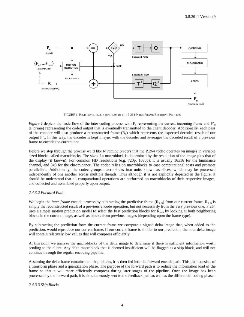
FIGURE 1: HIGH LEVEL BLOCK DIAGRAM OF THE P.264 INTER-FRAME ENCODING PROCESS

Figure 1 depicts the basic flow of the inter coding process with Fn representing the current incoming frame and F’n

(F prime) representing the coded output that is eventually transmitted to the client decoder. Additionally, each pass

of the encoder will also produce a reconstructed frame (Rn) which represents the expected decoded result of our

output F’n. In this way, the encoder is kept in sync with the decoder and leverages the decoded result of a previous

frame to encode the current one.

Before we step through the process we’d like to remind readers that the P.264 codec operates on images in variable

sized blocks called macroblocks. The size of a macroblock is determined by the resolution of the image plus that of

the display (if known). For common HD resolutions (e.g. 720p, 1080p), it is usually 16x16 for the luminance

channel, and 8x8 for the chrominance. The codec relies on macroblocks to ease computational costs and promote

parallelism. Additionally, the codec groups macroblocks into units known as slices, which may be processed

independently of one another across multiple threads. Thus although it is not explicitly depicted in the figure, it

should be understood that all computational operations are performed on macroblocks of their respective images,

and collected and assembled properly upon output.

2.4.3.2 Forward Path

We begin the inter-frame encode process by subtracting the predictive frame (Rn-m) from our current frame. Rn-m is

simply the reconstructed result of a previous encode operation, but not necessarily from the very previous one. P.264

uses a simple motion prediction model to select the best prediction blocks for Rn-m by looking at both neighboring

blocks in the current image, as well as blocks from previous images (depending upon the frame type).

By subtracting the prediction from the current frame we compute a signed delta image that, when added to the

prediction, would reproduce our current frame. If our current frame is similar to our prediction, then our delta image

will contain relatively low values that will compress efficiently.

At this point we analyze the macroblocks of the delta image to determine if there is sufficient information worth

sending to the client. Any delta macroblock that is deemed insufficient will be flagged as a skip block, and will not

continue through the regular encoding pipeline.

Assuming the delta frame contains non-skip blocks, it is then fed into the forward encode path. This path consists of

a transform phase and a quantization phase. The purpose of the forward path is to reduce the information load of the

frame so that it will more efficiently compress during later stages of the pipeline. Once the image has been

processed by the forward path, it is simultaneously sent to the feedback path as well as the differential coding phase.

2.4.3.3 Skip Blocks

3.8.2011 Version 9

5

Skip blocks are empty macroblocks that contain no information (other than identifying themselves as a skip). The

purpose of these blocks is to allow the encoder to notify the decoder when a macroblock contains no new

information and can simply be filled in with the associated predicted macroblock. When the encoder detects a skip

block it will:

1. Halt the processing of the block (it will not be processed by the feedback path).

2. Identify the skip block, along with any motion vectors, in the macroblock table (which is sent to the

decoder).

3. Instruct the predictive macroblock to propagate directly to the reconstructed image.

In this manner, we ensure that the reconstructed image always matches the decoded state even when skip blocks are

present.

2.4.3.3 Serialization

The differential coder is the first stage of the pipeline’s backend. This phase further reduces the information load of

the image by optionally transmitting the differences between subsequent macroblocks, rather than the blocks

themselves. In some cases, these differences will compress better than the original content. Next, the macroblocks

are presented to the Binarizer which is responsible for preparing macroblocks for compression. Depending upon the

frame type, either an Exponential Golomb code or a Run-Length code is generated. This code is then passed to a

context adaptive binary arithmetic coder (CABAC), which is a simple entropy coder that will compress the

macroblock into an efficient bit stream for output.

2.4.3.4 Feedback Path

The feedback path performs an inverse of the forward path. By adding this inverse to the current prediction we

derive a reconstructed frame that may be used to predict a future frame. The feedback path mimics the processing of

the decoder and produces a result that identifies the information lost during the forward path. As a result, each

subsequent frame delta will attempt to rectify this loss through refinement.

2.5 The Details

We now examine the pipeline in greater detail, beginning with image conversion and following with a review of the

codec. We place particular emphasis on any critical design considerations that had significant impact on the

performance and costs of this codec. Note that while the following steps are performed in a logically sequential

order, they may be optimized by the codec to run in parallel where possible. Additionally, please note that the data

layouts discussed in this paper are not necessarily the same as those used by the implementation, and that several

additional considerations have been taken by the codec to optimize the output bit stream.

3. IMAGE SPACE CONVERSION

The encoder expects input frames in a three channel YUV color space with chrominance sub-sampling using a 4:2:0

planar layout3. If the incoming data requires conversion, the server quickly processes it during this phase before

passing the frame to the encoder. This format is particularly appealing because it:

1. Allows the encoder to operate on the individual image planes as contiguous regions of memory.

2. Allows the encoder to traverse a smaller memory span during encoding.

3 Information about the YUV420 format is available at http://en.wikipedia.org/wiki/YUV.

3.8.2011 Version 9

6

3. Provides individual channel precision based on insights into human visual perception, which is more

sensitive to changes in luminance than changes in chrominance.

This format consists of an 8 bit per pixel luminance channel (Y), an 8 bit per pixel quad chrominance channel (U),

and a second 8 bit per pixel quad chrominance channel (V). Since the image is a planar format (as opposed to

interleaved), each channel is stored contiguously within its own image and is independently addressable4.

The luminance of a pixel is computed by taking the dot product of the source red, green and blue channels and a pre-

computed vector of conversion weights. Chrominance is slightly more complicated because it requires access to four

neighboring source pixels of a pixel quad to generate a single chrominance value. We compute the U and V

channels by taking the dot product of a weight vector and each of the four RGB values. We then average these four

results together and store the results in their respective chrominance channel.

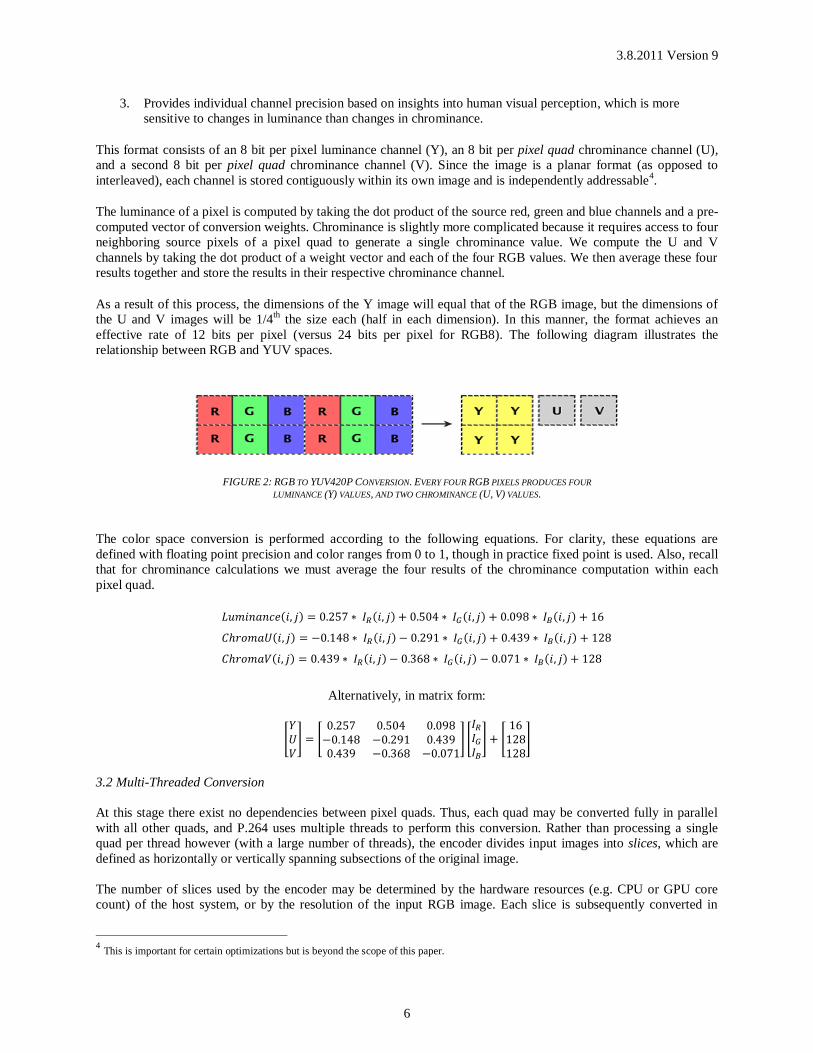
As a result of this process, the dimensions of the Y image will equal that of the RGB image, but the dimensions of

the U and V images will be 1/4th the size each (half in each dimension). In this manner, the format achieves an

effective rate of 12 bits per pixel (versus 24 bits per pixel for RGB8). The following diagram illustrates the

relationship between RGB and YUV spaces.

FIGURE 2: RGB TO YUV420P CONVERSION. EVERY FOUR RGB PIXELS PRODUCES FOUR

LUMINANCE (Y) VALUES, AND TWO CHROMINANCE (U, V) VALUES.

The color space conversion is performed according to the following equations. For clarity, these equations are

defined with floating point precision and color ranges from 0 to 1, though in practice fixed point is used. Also, recall

that for chrominance calculations we must average the four results of the chrominance computation within each

pixel quad.

( ) ( ) ( ) ( )

( ) ( ) ( ) ( )

( ) ( ) ( ) ( )

Alternatively, in matrix form:

[ ] [

] [

] [

]

3.2 Multi-Threaded Conversion

At this stage there exist no dependencies between pixel quads. Thus, each quad may be converted fully in parallel

with all other quads, and P.264 uses multiple threads to perform this conversion. Rather than processing a single

quad per thread however (with a large number of threads), the encoder divides input images into slices, which are

defined as horizontally or vertically spanning subsections of the original image.

The number of slices used by the encoder may be determined by the hardware resources (e.g. CPU or GPU core

count) of the host system, or by the resolution of the input RGB image. Each slice is subsequently converted in

4 This is important for certain optimizations but is beyond the scope of this paper.

3.8.2011 Version 9

7

parallel on a separate thread, thus forcing the encoding pipeline to yield until the entire image is converted and

assembled.

Alternatively, this conversion may be performed on the GPU by processing 4 RGB pixels per graphics thread (a

natural fit for most modern graphics processors).

4. MOTION ESTIMATION

After converting the current image into the YUV color space, it is ready to be processed by the encoder. We process

the macroblocks of the image sequentially (within each slice), and rely upon past information to improve our

efficiency. Given a current macroblock, the motion estimation phase will identify a prediction macroblock by

searching our set of previously reconstructed frames plus previously reconstructed blocks of the current frame to

find the closest match.

5. DELTA COMPUTATION

The next step is to subtract the current decoder output (represented by the motion predicted frame) from the current

frame. This will create a new “delta” image that can be added to the previously decoded frame on the client to carry

its visual state forward properly. In areas where the two images are relatively similar, the delta image will contain

low values which compress more efficiently than high values.

5.2 Prediction Frame

The prediction image used for comparison by this pipeline stage is computed using the output of the current decoder

state (presumably mirrored on a remote client). The encoder derives this by running the previous frame’s forward

path output through an in-place feedback path that mimics the behavior of the decoder.

The resulting image represents the current lossy output of our decoder and what should be currently visible on the

client. By subtracting this image from our current, the process captures a reasonable estimate of the error introduced

by the forward process, as well as the differences between adjacent frames in the video sequence.

6. SKIP BLOCK ANALYSIS

The skip analysis phase examines the delta frame, which is produced by subtracting prediction macroblocks from

the input blocks. The skip analysis determines whether sufficient information exists to justify its transmission to the

client decoder. The results of this comparison should minimally affect visual quality but are essential to the efficient

operation of the pipeline. If the current input macroblock is identical (or sufficiently similar) to the predicted block,

then no actual decoding is necessary and the client requires no update. Alternatively, if the macroblock contains a

significant delta, then the client must be informed and given the chance to decode the block.

6.2 Image Comparison

The process of qualifying a skip block looks for sufficiently similar pixel data. This determination of similarity is

flexible, and relies upon thresholds to optionally allow blocks with minor degrees of dissimilarity to still be

considered identical. The greater the thresholds, the more blocks will pass this test, thus lowering the computational

costs of encoding (by encoding fewer macroblocks), but increasing the error.

In addition to performing comparisons on a per-macroblock basis, this stage also performs comparisons

independently for each channel. This process prevents video sequences that display independently varying per-

channel color transitions from causing over quantization of lower frequency channels.

6.2.2 Comparison Internals

3.8.2011 Version 9

8

For each macroblock, a weighted image analysis operation is performed that determines the block-level degree of

inter-frame similarity. Any signed blocks that are entirely black (indicating no new information) will produce a zero

weighted result. Such a result may be produced by identical current and prediction blocks, or by forward path error

that has removed all information.

The encoder then uses a carefully chosen (and user provided) threshold to determine the amount of dissimilarity

required to flag a particular macroblock as a skip block.

6.2.3 Comparison Kernels

Macroblock pixel comparisons may be implemented in a variety of ways. The following list describes some of the

most common methods:

Simple Comparison (SCC)

Each pixel in the macroblock is compared with a zero value (indicating no delta). If all pixels in a macroblock

are black, then the block signifies that no change should occur between the current prediction and the current

reconstruction.

Sum of Squared Differences (SSD)

( ) ∑∑( ( ))

Each pixel in the block is squared and added to a running total. This final result will be zero for blocks that

represent no change, and increases with any divergence. A threshold is then used to tolerate small amounts of

discrepancies between the images that derived the signed frame.

In the equation above, is an image function that selects pixel (i,j) from macroblock x in the current delta image.

The summation limit m is assumed to define a symmetric macroblock dimension.

7. FORWARD PATH

After converting the current image into the YUV color space and subtracting the prediction, it is ready to be

processed by the forward path. The first phase of the forward path is the transformation into frequency space.

7.2 Frequency Transform

In order to provide a more efficient compression than directly encoded color data, each delta image macroblock is

transformed into the frequency domain by the (T) phase of the forward path. This process de-correlates pixel data

into its constituent frequency coefficients and allows us to independently quantize the frequency bands. For

example, we may discard high frequencies to remove subtle detail while preserving lower frequencies that convey

image structure. This first step is accomplished using a Fourier Transform for each macroblock. The following

equation details a forward Fourier Transform:

( ) ∫ ( )

A corresponding inverse Fourier Transform is expected within the feedback path in order to convert from the

frequency domain back into the appropriate color space. Note that Fourier transforms are often computationally

3.8.2011 Version 9

9

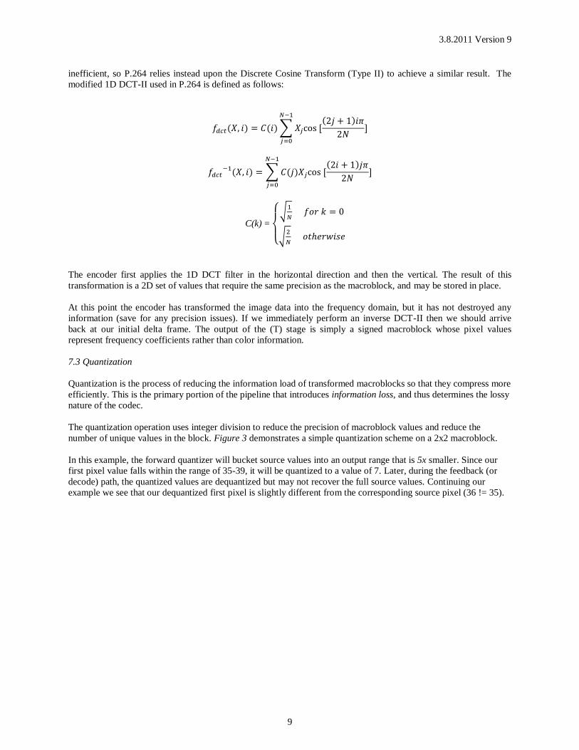
inefficient, so P.264 relies instead upon the Discrete Cosine Transform (Type II) to achieve a similar result. The

modified 1D DCT-II used in P.264 is defined as follows:

( ) ( ) ∑ ( )

( ) ∑ ( )

( )

C(k) =

{

√

√

The encoder first applies the 1D DCT filter in the horizontal direction and then the vertical. The result of this

transformation is a 2D set of values that require the same precision as the macroblock, and may be stored in place.

At this point the encoder has transformed the image data into the frequency domain, but it has not destroyed any

information (save for any precision issues). If we immediately perform an inverse DCT-II then we should arrive

back at our initial delta frame. The output of the (T) stage is simply a signed macroblock whose pixel values

represent frequency coefficients rather than color information.

7.3 Quantization

Quantization is the process of reducing the information load of transformed macroblocks so that they compress more

efficiently. This is the primary portion of the pipeline that introduces information loss, and thus determines the lossy

nature of the codec.

The quantization operation uses integer division to reduce the precision of macroblock values and reduce the

number of unique values in the block. Figure 3 demonstrates a simple quantization scheme on a 2x2 macroblock.

In this example, the forward quantizer will bucket source values into an output range that is 5x smaller. Since our

first pixel value falls within the range of 35-39, it will be quantized to a value of 7. Later, during the feedback (or

decode) path, the quantized values are dequantized but may not recover the full source values. Continuing our

example we see that our dequantized first pixel is slightly different from the corresponding source pixel (36 != 35).

3.8.2011 Version 9

10

FIGURE 3: QUANTIZATION OF A 2X2 PIXEL MACROBLOCK USING A CONSTANT

QUANTIZATION FACTOR OF 5.

In this example, the quantization factor of 5 was chosen arbitrarily. But in practice, this value is carefully configured

to balance compression efficiency with visual quality. The higher the quantization factor, the more error is

introduced into the image, thus lowering visual quality.

7.3.2 Jayant Quantization

P.264 uses a forward adaptive Jayant quantizer that is designed to reduce the precision of high frequencies while

preserving the low. Prior to any encoding operations, P.264 will build an array of quantization tables (each sized to

match our macroblock dimensions) called the quantization bank. This bank is then accessed during quantization to

supply per-pixel quantization factors. Each entry in the quantization bank is constructed with the following equation:

( )

( ) ( )

Based on this approach, the quantizer bank will consist of a high quality (low quantization factors) table in the first

bank, with progressively lower quality tables in each subsequent bank. Each table will also reduce quality non-

linearly such that low frequency coefficients are more closely preserved and high coefficients are more likely

discarded. Note that the constants a, b, c, and d are selected by the developer based on subjective reasoning about

the desired trade-off in quality vs. compression efficiency. The values presented here are purely for illustrative

purposes and may not match those employed by P.264.

7.3.2.2 Adaptive Quantization

During the forward quantization process, the encoder will select a table from this set and use it to quantize the

current macroblock. The actual quantization process is almost identical to that of Figure 3, except that the

3.8.2011 Version 9

11

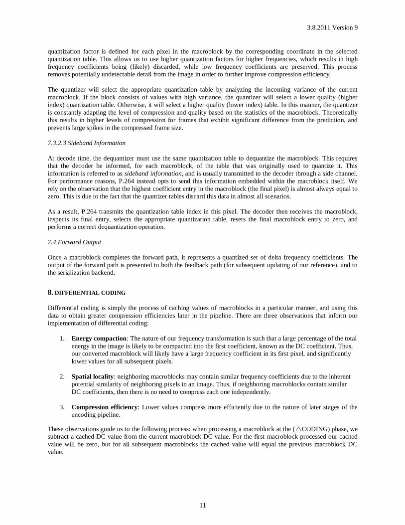
quantization factor is defined for each pixel in the macroblock by the corresponding coordinate in the selected

quantization table. This allows us to use higher quantization factors for higher frequencies, which results in high

frequency coefficients being (likely) discarded, while low frequency coefficients are preserved. This process

removes potentially undetectable detail from the image in order to further improve compression efficiency.

The quantizer will select the appropriate quantization table by analyzing the incoming variance of the current

macroblock. If the block consists of values with high variance, the quantizer will select a lower quality (higher

index) quantization table. Otherwise, it will select a higher quality (lower index) table. In this manner, the quantizer

is constantly adapting the level of compression and quality based on the statistics of the macroblock. Theoretically

this results in higher levels of compression for frames that exhibit significant difference from the prediction, and

prevents large spikes in the compressed frame size.

7.3.2.3 Sideband Information

At decode time, the dequantizer must use the same quantization table to dequantize the macroblock. This requires

that the decoder be informed, for each macroblock, of the table that was originally used to quantize it. This

information is referred to as sideband information, and is usually transmitted to the decoder through a side channel.

For performance reasons, P.264 instead opts to send this information embedded within the macroblock itself. We

rely on the observation that the highest coefficient entry in the macroblock (the final pixel) is almost always equal to

zero. This is due to the fact that the quantizer tables discard this data in almost all scenarios.

As a result, P.264 transmits the quantization table index in this pixel. The decoder then receives the macroblock,

inspects its final entry, selects the appropriate quantization table, resets the final macroblock entry to zero, and

performs a correct dequantization operation.

7.4 Forward Output

Once a macroblock completes the forward path, it represents a quantized set of delta frequency coefficients. The

output of the forward path is presented to both the feedback path (for subsequent updating of our reference), and to

the serialization backend.

8. DIFFERENTIAL CODING

Differential coding is simply the process of caching values of macroblocks in a particular manner, and using this

data to obtain greater compression efficiencies later in the pipeline. There are three observations that inform our

implementation of differential coding:

1. Energy compaction: The nature of our frequency transformation is such that a large percentage of the total

energy in the image is likely to be compacted into the first coefficient, known as the DC coefficient. Thus,

our converted macroblock will likely have a large frequency coefficient in its first pixel, and significantly

lower values for all subsequent pixels.

2. Spatial locality: neighboring macroblocks may contain similar frequency coefficients due to the inherent

potential similarity of neighboring pixels in an image. Thus, if neighboring macroblocks contain similar

DC coefficients, then there is no need to compress each one independently.

3. Compression efficiency: Lower values compress more efficiently due to the nature of later stages of the

encoding pipeline.

These observations guide us to the following process: when processing a macroblock at the (CODING) phase, we

subtract a cached DC value from the current macroblock DC value. For the first macroblock processed our cached

value will be zero, but for all subsequent macroblocks the cached value will equal the previous macroblock DC

value.

3.8.2011 Version 9

12

In this manner, the (CODING) phase will accept macroblocks of quantized frequency coefficients and produce

macroblocks in the same space, but with DC coefficients that merely represent the difference between the previous

macroblock DC and the current. This step results in much lower values for the first pixel in each block, and leads to

significantly greater coding efficiency.

9. BINARIZATION

Once macroblock values have completed the forward path and contain differential DC coefficients, they are ready to

be processed by the encoder backend and compressed into a bit-stream. This stage seeks to:

1. Merge macroblock content into a linear integer scale. Later stages of the pipeline expect input in the form

of a bit-stream, so we convert values where necessary and leverage a zig-zag access pattern to efficiently

convert our 2D macroblock data into a 1D stream.

2. Reduce the set of possible input values using a simple probability model and coding scheme.

The second step of this process is to convert the values into a more compact form using run length encoding and/or

exponential Golomb codes.

Some readers may note that this system pre-codes values just prior to submitting them to an arithmetic coder in the

very next phase, which may seem awkward at first. The reason for this design is that our arithmetic coder is an

adaptive binary coder, which simplifies some aspects of the codec design but also reduces its efficiency.

As a result, a pre-coding step is a useful way to reduce the number of tokens passed to the arithmetic encoder, and

promote better compression efficiency. One alternative to this system would be to use a multi-symbol arithmetic

coder with an accurate pre-calculated probability model, but that discussion is beyond the scope of this article.

9.2 Exponential Golomb Codes

Exponential Golomb codes were invented in 1960 by Solomon Golomb. They provide a simple way of reducing the

information load of a fixed sized integer array using variable length codes.

Problem: Given a series of 16 bit unsigned integers whose values are normally distributed about the

origin, device a coding scheme to reduce the overall size of the data.

What we’d like is a way to compress these values such that we avoid spending the full 16 bits per value, and

Golomb coding achieves this by assigning codewords to symbols. This system achieves our goal by assigning

shorter codewords to more frequent (i.e. lower) values, at the expense of assigning larger codewords to less frequent

(higher) values. We do not require the values to be normally distributed, as long as the frequency pattern is roughly

honored.

After a macroblock has been processed by the forward path, it contains values that are likely centered on the origin,

which matches our requirements for Golomb coding. Note that if this assumption is invalid, then Golomb coding

may not be the best choice of coding scheme (see run-length encoding below). Fortunately, most predictive frames

(p-frames) exhibit significant similarity to the reference and will present low macroblock values at this stage.

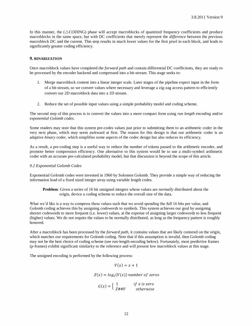
The unsigned encoding is performed by the following process:

( )

( ) ( ( ))

( ) {

3.8.2011 Version 9

13

Where ‘##’ represents the concatenation operator.

Coding of signed values is a simple extension of this process that alternates codes based on the sign of the input

value. The following table illustrates some of the most common unsigned codes:

Source Value Golomb Code

0 1

1 010

2 011

3 00100

4 00101

… …

9.3 Run Length Encoding (RLE)

For macroblocks that contain high repetition of high values, a run-length code will be more efficient than a Golomb

code. P.264 automatically detects this scenario and switches to run-length as necessary. A run-length code is

represented by two symbols, where the first symbol indicates a count and the second symbol indicates a value.

For example, if the sequence 000111 were to be encoded in this manner, the result would be 3031 to indicate a

sequence that consists of three zeroes followed by three ones. In most cases, Golomb codes are used due to the

likelihood of temporal and spatial locality in the images both within and across successive frames. However, when

the video sequence contains abrupt changes in visual content, a run-length code can produce a more optimal code.

9.4 Zig-Zag Pattern

The Golomb and run-length coding processes use a zig-zag access pattern when reading macroblock pixels. This

ordering was devised to maximize spatial similarity of data (i.e. similarity among neighboring pixels), which

benefits the run-length coder as well as the subsequent arithmetic coding phase. The zig-zag pattern is shown below

for a 4x4 macroblock:

FIGURE 4: PIXEL TRAVERSAL ORDER THROUGH A 4X4 MACRO-BLOCK DURING

FOURIER TRANSFORM (DCT-II) ANALYSIS.

10. ARITHMETIC CODING

Once each macroblock is transformed, quantized and pre-coded, it is ready to enter the compression phase of the

pipeline. At this stage, macroblocks are fed into an adaptive binary arithmetic encoder that has been tuned for video

compression.

This section provides a simple overview of adaptive binary arithmetic coding. We assume that the reader is familiar

with the more general concept of arithmetic coding5, so this discussion will only highlight the relevant extensions

5 http://en.wikipedia.org/wiki/Arithmetic_coding

3.8.2011 Version 9

14

for P.264.

Binary coding is a simplification of regular multi-symbol arithmetic coding. We use binary coding because it

simplifies our alphabet, reduces our cumulative distribution function to just a midpoint value (speeding up the

update process), and results in a much simpler stream process (you can begin decoding before encoding has

completed).

Unfortunately, these benefits come at a cost to coding efficiency because binary coders are unable to take advantage

of larger scale structure benefits that could otherwise reduce the number of codewords and symbols (see Extended

Huffman codes6 for a full explanation).

10.2 Binary Arithmetic Coding

As the name suggests, this binary arithmetic coder uses only two symbols, 0 and 1. This simplifies the coding

process and allows the encoder and decoder to operate without communicating a symbol set. Macroblocks are

processed as a bit-stream, one token (bit) at a time, and the results are collected within an output stream.

The coder is also adaptive and will continually adjust the probabilities of its binary symbols based on the actual

tokens that it processes. Since the encoder and decoder adapt in exactly the same manner, no sideband information is

necessary to communicate symbol probabilities.

10.2.3 Encode Process

Our encoding process begins with two initialization steps that are necessary to configure the coder. These steps

should only be performed at the beginning of each slice (and hence, at the start of each frame):

1. Set low to zero, high to our maximum value (e.g. 0xFFFF), and mid to our initial mid value (e.g. 0x7FFF).

2. Initialize our history to {1, 1} to represent probabilities for symbols {0,1} of {0.5,0.5}.

Using our example values (0, 0x7FFF, 0xFFFF) we’ve defined a 16 bit arithmetic coder with a coding range of 0-

0x7FFF for low and 0x8000-0xFFFF for high. Notice that, in this initial (and non-adaptive) state, our most

significant bit (MSB) distinguishes between our two ranges.

FIGURE 5: INITIAL RANGE OF THE ADAPTIVE ARITHMETIC CODER.

Once the encoder is initialized we can begin encoding symbols, one at a time, until we reach the end of a slice or

image. The process is as follows:

1. Resolve our model. This simply involves re-calculating our midpoint based on the high and low values. If

our coder was non-adaptive, then the midpoint would always simply be:

( )

Since our coder is adaptive, we must keep track of each token that is encoded and store totals for each

6 http://people.cs.nctu.edu.tw/~cjtsai/courses/imc/classnotes/imc12_03_Huffman.pdf

3.8.2011 Version 9

15

symbol. Thus, if our coder has previously processed the sequence 0001111, then our totals would be {3, 4}

to represent a history of three zeroes and four ones.

We use this history when we recalculate our midpoint because the midpoint represents the current

probability distribution of our symbols. In cases where our history contains an equal number of ones and

zeroes, then our computation matches that of the non-adaptive midpoint. Otherwise, our computation is the

following:

( )

2. Read the next bit from our input stream and adjust our low and high values based on the following:

Thus for each token we adjust either the high value, or the low value, but never both. We also increment

our history based on the token value.

3. Check for scaling. Similarly to generic arithmetic coding, we must examine our high and low values and

adjust them to avoid precision issues as our intervals shrink.

Once all symbols are encoded, we flush the encoder to complete our output.

10.3 Multi-Threaded Encoding

The process of encoding a bit-stream is a serial one due to the adaptive nature of the coder – the probability of the

next token relies upon the encoder having processed and adapted to the previous tokens. To compensate for this, and

enable multi-threaded encoding and decoding, P.264 uses a separate arithmetic coder instance for each slice of the

image. In this way, each slice is encoded or decoded independently of the other slices, and the result is accumulated

at the output.

11. CONCLUSION

The P.264 format is a simple codec that is designed to lower encode and decode latencies in exchange for higher

required bitrates. Based on beta surveys of our everyAir product, we’ve learned that switching from H.264 to our

custom codec has reduced, on average, our total encode plus decode time from around 35ms to 6ms (on 2010 mobile

hardware), and increased our bandwidth costs from 1.0 Mbps to 4.15 Mbps for 1024x768 30 Hz video. In real-time

video streaming scenarios, this tradeoff is likely to be acceptable as user tolerance to higher bandwidth is far less

elastic than user tolerance to higher latencies.