A logistics model for delivery of critical items in a disaster

relief operation: heuristic approaches†

Yen-Hung Lin a,b, Rajan Battaa,b,∗ , Peter A. Rogersona,c,Alan Blatta, Marie Flanigana

aCenter for Transportation Injury Research, CUBRC, Buffalo, NY 14225, United StatesbDepartment of Industrial and Systems Engineering,University at Buffalo (SUNY), Buffalo, NY

14260, United StatescDepartment of Geography,University at Buffalo (SUNY),

Buffalo, NY 14260, United States

Abstract

In this paper, a tour-based multi-objective logistics model for optimized scheduling of thedelivery of critical items in a disaster relief operation is proposed. Our model considersmulti-items, multi-vehicles, multi-periods, and a split delivery scenario in a disaster. Twoheuristic approaches are introduced to solve the logistics problem. In the first approach,a genetic algorithm is applied as the tour generator to filter out tours, to reduce the sizeof the problem. In the second approach, a vehicle assignment heuristic is proposed bydecomposing the original multi-vehicle, multi-location problem into several subproblemsconsisting of only a partial number of clusters in the main problem. Some randomlygenerated computational experiments are conducted to evaluate the performance of ourapproaches.

Key words: disaster relief, genetic algorithm, heuristics, split delivery

†This material is based upon work supported by the Federal Highway Administration underCooperative Agreement No. DTFH61-07-H-00023, awarded to the Center for Transportation InjuryResearch, CUBRC, Inc., Buffalo, NY. Any opinions, findings, and conclusions are those of theAuthor(s) and do not necessarily reflect the view of the Federal Highway Administration∗Corresponding author. Address: Department of Industrial and Systems Engineering, University

at Buffalo (SUNY), Buffalo, NY 14260, United States. Tel.: +1 716 6452357; fax: +1 716 6453302.E-mail address:batta@eng.buffalo.edu (R. Batta)

Preprint submitted to Transportation Research Part E April 30, 2009

1. Introduction

In recent years, much human life has been lost due to natural disasters. For

example, at least 1,836 people lost their lives in Hurricane Katrina in 2005, and

73,276 died in the Kashmir Earthquake in Pakistan in 2005. To mitigate damage

and loss in disasters, studies in pre-disaster, during disaster, and after-disaster issues

have been widely explored in the past few years. One of the critical challenges is to

transport sufficient critically needed supplies to affected areas in order to support

basic living needs to those who are isolated in disaster-affected areas. Normally,

daily living needs include water, food (e.g., ready-to-eat meals), medicine, and other

equipment (e.g., blankets, tents, etc.). Usually, disaster relief operations are initiated

immediately after the occurrence of the disaster and continue until all stranded people

are completely rescued and the basic living infrastructure (e.g., communications,

power supplies, water supplies, or transportation system) is renewed. Since the

demand required during and after a disaster is usually large and unexpected, and

resources, e.g. supplies or transportation vehicles, are normally limited, a good

logistics plan is absolutely necessary to transport supplies from distribution centers to

targeted locations. Therefore, it becomes a critical, but difficult task for authorities

to make fast and correct logistics decisions.

A disaster relief operation is usually executed by mixing different types of trans-

portation mediums (e.g., vehicles, boats, or helicopters) and assigning them to deliver

supplies to meet demands requested in different locations. We note that for our study

we restrict attention to just vehicles as the transport mode. If vehicles are used, the

existing surface transportation network (e.g., highway systems, roads, etc.) is used.

All vehicles depart from a distribution center or depot with fully loaded supplies and

2

travel to one or more locations to deliver those supplies, and then come back to the

distribution center to reload supplies and wait for the next assignment. Specifically,

a tour is the unit used in this study to describe the movement of a vehicle in an

assignment. Two decisions have to be made in a tour assigned to a vehicle: 1) how

many locations will be visited, and the order of the visiting, and 2) what supplies will

be carried by the vehicle. Equivalently, two types of information should be addressed

in a disaster relief operation, where the demand requests come from, and what types

of supplies are required.

In our study, a distinguishing feature is to consider different types of critical items

in a disaster relief operation. Based on human survival needs, medicine, water, and

food are the three most critical items, and these are included in our study. Since

critical items are not all needed equally, differentiation of urgent levels for these

three items should be considered. In other words, the most urgent item should

always be given the highest delivery priority, even though it may cause delays for

other items. To implement this idea, a penalty cost is employed for each item if it

cannot be delivered on time. Delivery on time means that the requested amount

of an item is delivered within the allowable time period, which is predefined based

on the characteristic of items. For example, people cannot survive without drinking

water for 48-72 hours; thus, the requested demand of water in a location cannot be

delayed more than 48-72 hours. A penalty cost is given if it takes longer than 72

hours to satisfy the demand. A similar idea is applied to the two other items.

The delivery of critical items in a disaster relief operation is similar to the con-

ventional vehicle routing problem (VRP), however, the characteristic of a disaster

relief operation doesn’t completely conform to the VRP, since demand in a location

3

is not likely to be satisfied by a single vehicle in a single delivery. Fortunately, one of

the special cases in the VRP, the Split Delivery Vehicle Routing Problem (SDVRP),

is suitable to describe our scenario. The key is that in the SDVRP, the demand from

a customer can be fulfilled by more than one vehicle. In a disaster relief situation

with different priority items, split delivery becomes a good strategy not only it is

inevitable to deal with a large demand in a short time period, but it is also useful to

allow decision makers to focus on those high priority items.

In addition to considerations of item characteristics, multiple objectives are taken

into account in the study. Minimizing total travel cost is a typical objective which is

used in transportation-related problems, e.g. the vehicle routing problem. However,

in the emergency scenario, minimizing unsatisfied demand is important. A conflict

exists between these two objectives. For example, the best way to reduce unsatisfied

demand is to sent more vehicles to deliver supplies to demand locations; however, it

is usually not allowed due to limitations of the number of vehicles and the budget

for transportation of relief supplies. Consequently, the trade-off among different

objectives becomes a critical challenge for decision makers, especially when they are

making complicated decisions such as disaster relief operations, because any decision

will have an immense impact on numerous victims in a disaster.

Based on the above analysis, we propose a multi-objective integer programming

model to solve the delivery problem in the disaster relief scenario. The characteristics

of our problem include a limited number of vehicles in a multi-period, multi-item

environment. Since real disaster relief operations are usually complicated, large-

scale integer programming problems, it is a NP-hard problem from the perspective

of optimization. Therefore, two heuristic approaches are introduced in this study.

4

The first approach is to generate some useful tours based on genetic algorithms;

then, in the second approach, a vehicle assignment heuristic approach is designed

to appropriately divide vehicles to serve different clusters. Furthermore, since our

problem is represented by a multi-objective integer programming model, methods of

multi-objective optimization are adopted to help decision makers make more reliable

decisions among different objectives.

The rest of this paper is organized as follows. Section 2 provides a review of the

literature related to our research. Section 3 presents the mathematical formulation of

the multi-objective integer programming model for the critical items delivery problem

in disaster relief. Two heuristic approaches are introduced in Section 4 to solve this

problem. In Section 5, the methods of multi-objective optimization in our study

are described. Then, some computational experiments and results are provided and

discussed in Section 6. Finally, Section 7 contains conclusions and suggestions for

future work.

2. Literature Review

In the first subsection, literature on disaster relief operations is reviewed, espe-

cially that related to logistics planning. An overview of research in the Split Delivery

Vehicle Routing Problem (SDVRP) is provided in the second subsection because it

is much more similar to the disaster relief scenario.

2.1. Disaster Relief Operations

In the past few years, more and more studies of disaster relief operations have

drawn attention and appeared in the literature. Two general types of topics are

5

usually explored in the research on disaster relief. The first type of research is related

to rescue and transport casualties after the disaster, while the second type is focused

on logistics problems to deliver supplies into the disaster-affected areas, intending to

mitigate the potential casualties due to lack of supplies (i.e., food, water, medicine).

Gong and Batta (2007) considered ambulance allocation and reallocation models

for a diaster relief operation. The initial problem is focused on allocating the cor-

rect number of ambulances to each cluster at the beginning of the recsue operation.

Then, the second problem considers ambulance allocation to serve new clusters and

fully utilize ambulances. Jotshi et al. (2009) developed a methodology for the dis-

patching and routing of emergecy vehicles in a disaster environment. They modeled

the problem including dispatch and routing of emergency vehicles to casualty pickup

locations, and followed by delivery to appropriate hospitals.

In addition to the first type of research in disaster relief operations, more research

focuses on the logistics problem in a disaster scenario. Fiedrich et al. (2000) proposed

a dynamic optimization model to find the best assignment of available resources to

operational areas after earthquake disasters. The objective is to minimize the total

number of fatalities during the initial search-and-rescue period after strong earth-

quakes. Barbarosoglu et al. (2002) developed a mathematical model for assigning

helicopters tasks during a disaster relief operation. They decomposed the decision

problem into two sub-problems. The top level sub-problem was used to make tactical

decisions, i.e. assigning helicopters from the air force bases to the operation base,

while the base level sub-problem was used to decide operational routing and loading

decisions.

Ozdamar et al. (2004) proposed an emergency logistics planning model for nat-

6

ural disasters. The model they proposed addressed the dynamic, time-dependent

transportation problem, and this problem is solved repetitively at given time peri-

ods. In addition, another approach to emergency logistics distribution in a disaster

relief operation was introduced by Sheu (2007). The approach he proposed was

based on a hybrid method, including fuzzy clustering and multi-objective dynamic

programming models.

Furthermore, there is some research considering both casualty pickup and supply

delivery problems. Yi and Odamar (2007) proposed a dynamic logistics coordination

model for both evacuation and support in disaster relief operations. A two stage

methodology was employed: the first stage was used to minimize the delay in the ar-

rival of commodities and in the healthcare for injuries, and the second stage detailed

vehicle instructions to assign a loading and unloading schedule to each itinerary. Yi

and Kumar (2007) proposed the ant colony optimization approach for disaster relief

operations. The operations they were considering included dispatching commodi-

ties to distribution centers around the affected areas and evacuating the injuries to

medical centers. In their approach, they decomposed the original problem into two

subproblems and solved them in an iterative manner.

A study comparable to ours is found in Balcik et al. (2008); they considered a

tour-based last mile distribution system. The “last mile” means the final stage of a

humanitarian relief chain. Their study focused on allocating relief supplies among

demand locations and determining delivery schedules for each vehicle in the planning

horizon. However, in their study, the tour they determined was based on solving

a Traveling Salesperson Problem (TSP). In contrast, there is no limitation on the

number of locations where a vehicle has to visit in our study because, from a practical

7

viewpoint, it is usually difficult to assign vehicles to travel to too many locations,

because vehicle capacity is relatively smaller than the demand in any single location.

Another consideration different from theirs is that backorders of regularly consumed

items (i.e., food) were not allowed, and unsatisfied demand was lost, while, in ours,

we consider the backorder scenario, and unsatisfied demand will not only accrue a

penalty cost, but also be accumulated to the next period until it has been satisfied. In

fact, a challenging task in our study is to handle the fact that all unsatisfied demands

of various items are continuously monitored during the entire planning period. A

detailed explanation of this will be given in the next section.

2.2. Split Delivery Vehicle Routing Problem

The split delivery vehicle routing problem (SDVRP) was first proposed by Dror

and Trudeau (1989). They showed that benefits could be expected through split

deliveries both on total travel distance and the number of vehicles required. Fur-

thermore, Dror et al. (1994) proposed an integer programming formulation and in-

troduced several valid inequalities. A branch and bound algorithm was proposed in

their research to solve the SDVRP. Frizzell and Giffin (1992, 1995) developed the

extension of the SDVRP with time windows and grid network distances. Two im-

proved heuristics approaches had been proposed in their studies, where one was to

move customers between routes, and another was to exchange customers between

routes.

Although not many studies have been published in the literature since the SDVRP

was introduced, the SDVRP has drawn a lot of attention since 2000. Some theoretical

research has appeared in the literature to investigate the characteristics of the split

8

deliveries. Belenguer et al. (2000) proposed a lower bound for the SDVRP according

to a polyhedral study of the problem. They used a cutting-plane algorithm for

small size instances. Bompadre et al. (2006) presented the lower bound for the VRP

with and without split deliveries. Based on the lower bound they presented, they

developed the quadratic iterated tour partitioning and the quadratic unequal iterated

tour partitioning heuristics for the SDVRP. Archetti et al. (2006a) performed a worst-

case performance analysis of the SDVRP. They concluded that the maximum cost

savings that can be realized is at most 50%. Recently, Archetti et al. (2008) used an

empirical study and again showed that the largest benefits are obtained when average

customer demand is just over 50% of the vehicle capacity and when the variance of

customer demand is relatively small.

In addition to theoretical research, solution approaches and applications have

been studied. Ho and Haugland (2004) have developed a tabu search algorithm to

solve the SDVRP, with a time window. Three steps were included in their approach.

In the first step, they computed a feasible solution simply based on the traveling and

waiting times; then, they improved the solution by using the tabu search algorithm

with some move operators; finally, they excluded the splitting option in the third

step to see if an improved solution could be found. The tabu search algorithm was

also employed in Archetti et al. (2006b) for the SDVRP. Their approach was based

on neighbor search in each iteration by removing a customer from a set of routes, and

by inserting it either to a new route, or into an existing route with extra capacity.

Jin et al. (2007) proposed a two-stage algorithm with valid inequalities to solve the

SDVRP. The first stage created clusters to cover all demand and established a lower

bound. In the second stage, the minimal distance traveled for each cluster was

computed by solving the traveling salesman problem. Later, Jin et al. (2008) applied

9

column generation to solve the same problem with large demands. For some other

application-oriented studies, interested readers can refer to Archetti et al. (2005);

Chuah and Jon (2005); Nowak et al. (2008); and Ohlmann et al. (2008).

3. Disaster Relief Logistics Model

3.1. Assumption

The problem considered in this study is to deliver relief supplies to disaster-

affected areas immediately after a disaster occurs, and to do so for a specific number

of time periods. Multiple locations scattered around the disaster area are required to

be served by a single distribution center (depot). The demand locations are clusters

which are used to receive supplies from the distribution center and they then dis-

tribute them house by house in their neighborhood. It is presumed that the supplies

are unlimited in the distribution center and that the demand requests from various

clusters can be correctly estimated before the beginning of the planning horizon in a

relief operation. The total demands are usually estimated according to the number

of people who are affected in the neighborhood of each cluster, and are not required

to be transported to hospitals or medical centers to get further medical treatment.

For modeling simplicity, demand is assumed unchanged during all planning time pe-

riods. Three types of supplies (medicine, water, and food) are identified as basic

items, and are required to be delivered to clusters via the transportation network.

Urgency levels of items are differentiated based on their importance. We assume

that the delivery of medicine is the highest priority, followed by delivery of water

and then food.

10

In addition, characteristics of the transportation mode and the delivery meth-

ods are considered. Multiple but limited numbers of identical vehicles are used to

transport critical items. Vehicle capacities are limited, both on weight and volume,

according to manufacturers’ specifications. For each vehicle, tours are assigned in

each period to deliver items to one or more clusters. Tours begin at the depot,

continue to one or multiple clusters, and then return to the depot. For this study

we assume the total working hours for the operation are limited to 12 hours a day.

Therefore, the total travel time required to travel all predetermined clusters in any

tour cannot exceed the constrained number of working hours. The analyses do not

consider the time to load and unload items on or off the vehicle. Furthermore, any

cluster can be served multiple times by a single vehicle or multiple vehicles, and

demand can also be satisfied fully or partially in a single delivery. In other words,

multiple deliveries of any type of item in a single cluster are allowed in our prob-

lem. Therefore, it can be regarded as a split delivery vehicle routing problem in our

application.

3.2. Multi-Objective Logistics Model

Based on the above assumptions and general descriptions of the scenario, the relief

delivery problem can be constructed by an integer programming model. In particular,

three objectives are taken into account in this problem. Before introducing the

mathematical formulation, notation, parameters and decision variables are defined

below.

11

3.2.1. Notation, Parameters, and Decision Variables

Notation and Parameters:

i: the index of the supplies in the set of I = {medicine, water, food};

j: the index of the cluster in the set J = {1, 2, 3, . . . , , j};

k: the index of tours in the set K = {1, 2, 3, . . . , k};

l: the index of vehicles in the set L = {1, 2, 3, . . . , l};

t, n,m: the index of time period in the planning horizon;

T : the total planning periods;

v: the index of periods when the backorder amount of demand is delivered ;

u: the index of severe level of delay;

Jk: the set of locations which the vehicle will visit on tour k;

dijt: demand of the supply i at cluster j in time t;

piu: penalty of item i if the severe level of delay is u;

tk: travel time required for the tour k;

toi: tolerated delay time of item i;

ai: unit weight of item i;

bi: unit volume of supply i;

Ck: total travel cost in tour k;

H: total working time available in a single period;

W : the maximum load weight of a vehicle;

V : the maximum volume capacity of a vehicle;

M : a big number; and

S: difference of satisfaction rate between any two clusters;

sj: satisfaction rate in cluster j.

12

Decision Variables:

xijklt: amount of item i delivered at cluster j on tour k by vehicle l in period t;

wijklmn: amount of item i delivered at cluster j on tour k by vehicle l in period m

to satisfied demand in period n, where m,n ∈ T ;

and

yklt: equal of one when tour k is assigned to vehicle l in period t, and 0 otherwise.

3.2.2. Formulation

Objective 1:

min.

Z1 =∑

i

∑j

T−toi∑u=1

T−toi−u+1∑t=1

(dijt −

∑k

∑l

(xijklt +

t+u∑v=t+1

wijklvt

))· piu+

∑i

((∑j

∑t

dijt −∑

j

∑k

∑l

∑t

(xijklt +

∑m>t,m∈T

wijklmt

))· pi1

) (1)

Objective 2:

min. Z2 =∑

k

∑l

Ckyklt (2)

Objective 3:

min. Z3 = S (3)

where

S = max {|sp − sq|} , ∀p, q ∈ j, p 6= q

sj =

∑i

∑k

∑l

∑t

(xijklt +

∑m>t,m∈T wijklmt

)∑

i

∑t dijt

(4)

13

Subject to:

∑k

tkyklt ≤ H ∀l,∀t (5)

xijklt ≤Myklt ∀i,∀j ∈ Jk,∀k,∀l,∀t (6)

wijkltn ≤Myklt ∀i, ∀j ∈ Jk,∀k, ∀l,∀t,∀n < t (7)∑k

∑l

∑t

xijklt +∑

k

∑l

∑m>t,m∈T

∑t

wijklmt ≤∑

t

dijt ∀i,∀j (8)

∑i

∑j

ai

(xijklt +

∑n<t,n∈T

wijkltn

)≤ W ∀k,∀l,∀t (9)

∑i

∑j

bi

(xijklt +

∑n<t,n∈T

wijkltn

)≤ V ∀k, ∀l,∀t (10)

xijklt ≥ 0 ∀i,∀j ∈ Jk,∀k,∀l,∀t (11)

wijklmn ≥ 0 ∀i, ∀j ∈ Jk,∀k,∀l,∀m ∈ T,∀n ∈ T (12)

xijklt = 0 ∀i,∀j /∈ Jk,∀k,∀l,∀t (13)

wijklmn = 0 ∀i, j /∈ Jk,∀k,∀l,∀m ∈ T,∀n ∈ T (14)

yklt ∈ {0, 1} ∀k, l, t (15)

In this model, the objective function (1) is a penalty function that aims to min-

imize unsatisfied demand after the relief operation in this period. There are two

parts in this objective function. The first part (before the plus sign) indicates the

total accrued penalty cost, which is the sum of penalty cost for various severe delay

levels during the planning periods, and the second part is the penalty cost accrued

14

at the end of the planning periods. This objective function attempts to minimize

total unsatisfied demand, especially for high priority items. The objective function

(2) aims to minimize the total travel time for all tours and all vehicles. The purpose

of this objective is to assign as many vehicles as possible during the working hour

limitation in order to deliver the largest amount of items (this assumes that the de-

mand in a disaster scenario will be large). Objective function (3) is used to minimize

the difference in the satisfaction rate between clusters. The satisfaction rate is the

ratio between the requested demand and the actual delivered amounts. The pur-

pose of this objective is intent on balancing the service among clusters. “fairness”

is the term usually used to describe this purpose. In addition to these objectives,

equation (4) is the constraint used to calculate the difference in the satisfaction rate

between any pair of clusters. Equation (5) indicates that the total travel time of all

tours assigned to any single vehicle in this period cannot be longer than the available

working hours in a single period. Equation (6) shows that delivery units of items

only can exist if corresponding tours are selected to deliver supplies. Equation (8)

shows that the total delivery amount of items cannot exceed the demand during the

planning periods. Equations (9) and (10) are capacity constraints of a vehicle which

are the total available loading weight limit and the total volume limit, respectively.

Equations (11) - (14) are used to ensure that vehicles can only stop and deliver to

clusters on tours assigned to them. Finally, equation (15) indicates yklt is a binary

variable.

3.3. Properties of the Model

Since our problem is a variant of the split delivery vehicle routing problem, it is

anticipated that our model can also benefit from properties of the SDVRP (Dror and

15

Trudeau 1989, 1990, Dror et al. 1994). In this section, we will prove these properties

are valid in our multi-objective logistics model.

First of all, if the travel cost {cpq} , p, q ∈ J satisfies the triangular inequality,

then the following theorem holds:

Theorem 1. In any optimal tour collection, no two tours can have more than one

split demand cluster in common.

Proof. (by contradiction) Suppose that the theorem does not hold. Then in any

optimal tour collection Y ∗, there exists two tours that have more than one spit

demand cluster in common. Consider such a solution Y ∗∗, in which tours r1 and r2

are visited by the same vehicle to two split delivery clusters p and q, p 6= q. In tour

r1, we deliver δ1ip to cluster p and δ1

iq to cluster q. In tour r2 we deliver δ2ip to cluster

p and δ2iq to cluster q.

Because these deliveries must satisfy the weight and valume constraints for the

vehicle, we have∑

i

∑j=p,q aiδ

kij ≤ W , and

∑i

∑j=p,q biδ

kij ≤ V , k = 1, 2. Without

loss of generality, suppose δ1ip = min

{δ1ip, δ

1iq, δ

2ip, δ

2iq

}, ∀i, we now show that the same

delivery amount of items in these two tours can be achieved by visiting only cluster

q in tour r2. For this new steup,

δ̂1ip = 0,∀i

δ̂1iq = δ1

iq + δ1ip,∀i

δ̂2ip = δ2

ip + δ1ip,∀i

δ̂2iq = δ2

iq − δ1ip,∀i.

16

We can verify the continued satisfaction of the weight and volume constraints by

noting that:

∑i

∑j=p,q

aiδ̂1ij =

∑i

aiδ̂1ip +

∑i

aiδ̂1iq

= 0 +∑

i

aiδ1iq +

∑i

aiδ1ip

=∑

i

∑j=p,q

aiδ1ij ≤ W,

and

∑i

∑j=p,q

biδ̂1ij =

∑i

biδ̂1ip +

∑i

biδ̂1iq

= 0 +∑

i

biδ1iq +

∑i

biδ1ip

=∑

i

∑j=p,q

biδ1ij ≤ V,

and

∑i

∑j=p,q

aiδ̂2ij =

∑i

aiδ̂2ip +

∑i

aiδ̂2iq

=∑

i

aiδ2ip +

∑i

aiδ1ip +

∑i

aiδ2iq −

∑i

aiδ1ip

=∑

i

∑j=p,q

aiδ2ij ≤ W,

17

and

∑i

∑j=p,q

biδ̂2ij =

∑i

biδ̂2ip +

∑i

biδ̂2iq

=∑

i

biδ2ip +

∑i

biδ1ip +

∑i

biδ2iq −

∑i

biδ1ip

=∑

i

∑j=p,q

biδ2ij ≤ V.

Suppose S1 and S2 are solutions of the original delivery strategy and the new delivery

strategy, and Z1 = {z11 , z

12 , z

13} and Z2 = {z2

1 , z22 , z

23} are corresponding objective

values of three objectives as (1) - (3). Since the delivery quantities of various items

to the two clusters remain the same, the penalty cost due to unsatisfied demand and

the satisfactory rates in each cluster are unchanged. Therefore, z11 = z2

1 and z13 = z2

3 .

However, the total travel cost is reduced because the new tour has fewer clusters to

visit and due to the triangular inequality assumption. We can conclude that Z1 is

dominated by Z2, contradicting the optimality of Y ∗. The theorem follows.

Definition 1. Suppose there exist k distinct clusters l1, . . . , lk and k tours in the

optimal tour collection Y ∗. r1 includes cluster l1 and l2, r2 includes cluster l2 and

l3, . . . , and rk includes cluster lk and l1. The collection of clusters {li}ki=1 is called a

k -split cycle.

Theorem 2. In the multi-objective logistics problem, there is no k-split cycle tours

in the optimal tour collection Y∗, for any k ≥ 2

Proof. Omitted for the sake of brevity, as its proof follows a very similar argument

to that used in the proof of Theorem 1.

18

The benefit of Theorems 1 and 2 is significant when we propose one of our ap-

proaches. The explanation will be provided in section 4.2.5.

4. Heuristic Approaches

4.1. Challenge and Strategy of Optimization

As shown in the model above, two important parameters are the set of tours and

the number of vehicles. For a small relief logistics problem (e.g., only 3 or 5 clusters),

enumerations of all possible tours are still practicable. However, as the number of

clusters increases, the number of possible tours increases exponentially. Although

the limitation on working time is helpful in eliminating some infeasible tours that

require too much travel time, the number of remaining tours is still very large.

The number of vehicles is another issue to consider. More vehicles used in disaster

relief operations means more assignment decisions have to be made. Therefore,

the following two questions emerge when facing a large scale problem: 1) How can

we make sure all feasible tours are included in the mathematical model?, and 2)

can the optimization software (e.g., CPLEX) solve the problem with so many tours

and vehicles included? Unfortunately, both questions have negative answers. To

overcome these deficiencies, two heuristic approaches are introduced here; they are

based on reducing the number of vehicles, or reducing the number of tours in the

model, or both.

In the first approach, we try to reduce the number of tours required in the mathe-

matical model. A tour generator is employed to generate a set of tours as parameters

in the mathematical model. For practical purpose, the number of tours in the set

19

is usually limited to a small number (e.g., 10). The approach we used in the tour

generator is based on the genetic algorithm. The results from the tour generator are

a set of “good” tours that is believed will produce an approximately optimal solu-

tion. In the second approach, a vehicle assignment heuristic approach is developed

to assign vehicles to different clusters appropriately, in order to reduce the number

of vehicles used in the model. The assignment will be performed geographically, in

order to shorten the distance that vehicles travel. In other words, geographical areas

will be divided into small geographical blocks, and a partial number of vehicles will

be assigned to one of these blocks. The details of our approaches are illustrated in

the following subsections.

4.2. Tour Generation Approach

As described above, enumerating all tours becomes impractical and also increases

the difficulty of solving problems when the number of clusters becomes large. There-

fore, a “tour generator” is proposed to rectify this deficiency as our first approach.

The tour generator is used to generate a set of a small number of tours each time as

parameters in the mathematical programming model. It will iteratively generate a

set of tours and interact with the mathematical model to evaluate the performance

of various combinations of tours. To generate a set of “good” tours efficiently, a

meta-heuristic approach is employed. Among meta-heuristic approaches that have

been developed and applied in the literature, genetic algorithms (GA) are one of

the popular and powerful meta-heuristic methods. In the past, some studies have

appeared in the literature to propose how to apply genetic algorithms to vehicle

routing problems (Baker and Ayechew 2003, Ho et al. 2008, Prins 2004, Silva et al.

2008). The nature of Genetic Algorithms is a good fit for our purpose, because it is

20

an effective method to explore the solution space globally and converge on a group

of good solutions (or tours) in our application.

GA starts with an initial group of randomly selected solutions corresponding to

the problem, called the population, and each solution in the population is called

a chromosome. In the tour generator, a chromosome is a set of a limited number

of tours that is used to feed into the mathematical model shown in the previous

section. Chromosomes evolve iteratively, and each evolution is called a generation.

As shown in Figure 1, in each generation, chromosomes in the population, called

parents, are evaluated to determine the quality of each chromosome. All of them are

going through selection, crossover, and mutation processes to produce children. The

feasibility test and enforced mutation are performed to make all children valid. Then,

these children are evaluated and compared with their parents in order to eliminate

some less effective children. The identical number of chromosomes as the previous

population is selected among parents and children to constitute the population in the

next generation. The procedure is repeated until a predefined number of iterations

has run. The measure of evaluation of a chromosome is usually called the fitness

value, and this is defined according to various applications. Further discussions of

individual operations in this procedure are now provided.

4.2.1. Initialization

The chromosome representation is used to represent the tours used in the math-

ematical model. Each chromosome consists of a set of tours, the number of which is

defined arbitrarily. The tradeoff is that if more tours are generated, more computa-

tional effort is expected to optimize the problem, while if only a few tours are used,

21

Figure 1: Flowchart of Genetic Algorithm

it is unlikely to produce the optimal tour combination. The visited clusters in each

tour are also defined according to different purposes. In our case, we assume that

the demand in each single cluster is usually very large as compared to the assumed

vehicle capacities; therefore, it is improbable for vehicles to visit many clusters in a

single tour. Based on our experiments, 1 to 3 clusters in a single tour is reasonable.

It should be clarified that this number is greatly influenced by different factors, i.e.,

demand, the capacity of vehicle, the network, etc. The representation of the chro-

mosome in our study is shown in Figure 2. This chromosome is designed for five

clusters. The first row is the reference row, and is used to indicate the number of

22

Figure 2: An Example of Chromosome Representation

clusters in the corresponding tour (i.e., the first tour is only required to visit one

cluster, and the cluster assigned to this tour is “2”). It is noted that this row will

not be included in the genetic operations during the procedure. Therefore, suppose

“0” indicates the depot; there is a total of six tours in this chromosome, (0-2-0),

(0-1-0), (0-5-0), (0-3-4-0), (0-3-2-0), and (0-1-4-5-0).

In the initial step of the GA, a set of chromosomes is generated to form a popula-

tion that usually consists of 20-50 chromosomes. Suppose there are k tours included

in each chromosome for a j cluster problem, and the number of clusters visited in

each tour is ci, i = 1, . . . , k, respectively. Then there is a N ×∑

i ci matrix as the

initial population in the GA, where N is the size of the population. We applied the

nearest neighborhood principle to generate the initial population. Initially, a cluster

is randomly selected; then the closest cluster is selected to be the next following clus-

ter in the chromosome from those unselected clusters until all clusters are selected.

The procedure is repeated until all positions in a chromosome are filled. Following

the same method, N chromosomes can be generated, and the initial population is

obtained.

23

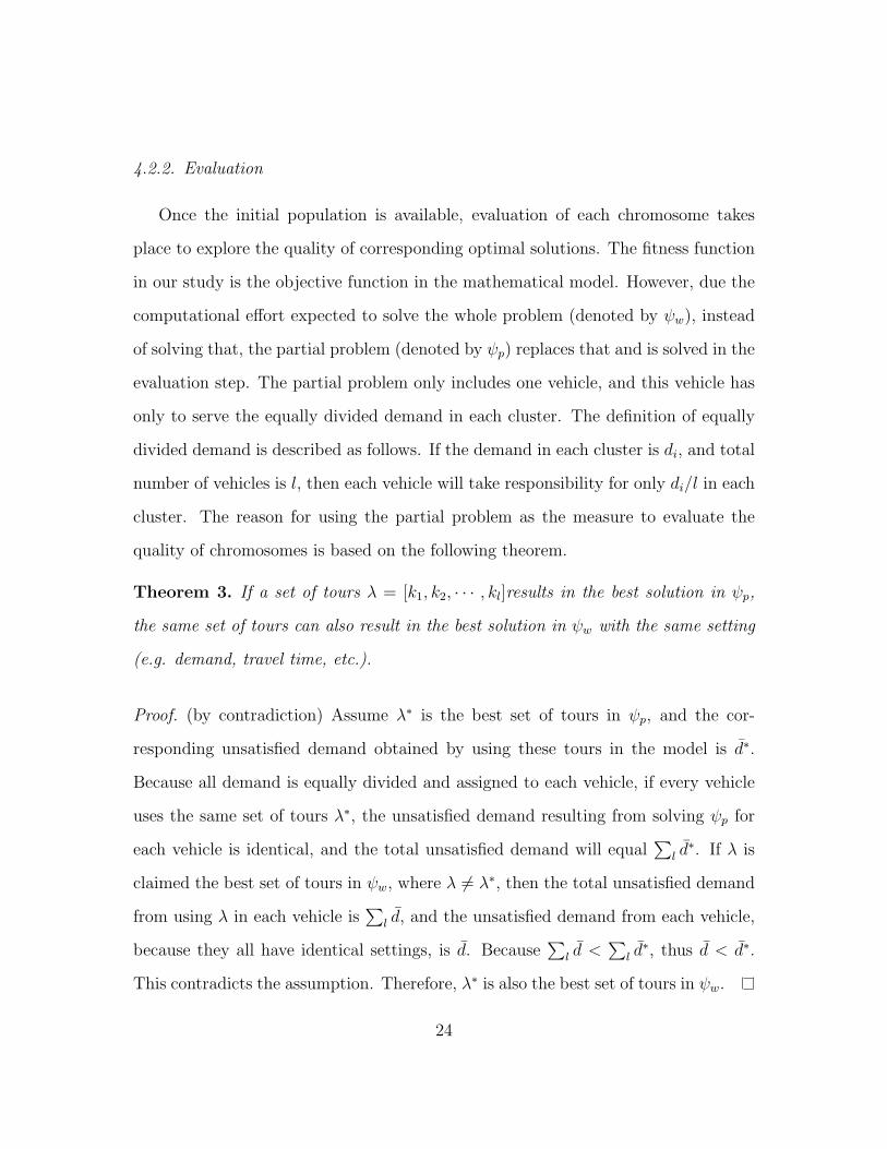
4.2.2. Evaluation

Once the initial population is available, evaluation of each chromosome takes

place to explore the quality of corresponding optimal solutions. The fitness function

in our study is the objective function in the mathematical model. However, due the

computational effort expected to solve the whole problem (denoted by ψw), instead

of solving that, the partial problem (denoted by ψp) replaces that and is solved in the

evaluation step. The partial problem only includes one vehicle, and this vehicle has

only to serve the equally divided demand in each cluster. The definition of equally

divided demand is described as follows. If the demand in each cluster is di, and total

number of vehicles is l, then each vehicle will take responsibility for only di/l in each

cluster. The reason for using the partial problem as the measure to evaluate the

quality of chromosomes is based on the following theorem.

Theorem 3. If a set of tours λ = [k1, k2, · · · , kl]results in the best solution in ψp,

the same set of tours can also result in the best solution in ψw with the same setting

(e.g. demand, travel time, etc.).

Proof. (by contradiction) Assume λ∗ is the best set of tours in ψp, and the cor-

responding unsatisfied demand obtained by using these tours in the model is d̄∗.

Because all demand is equally divided and assigned to each vehicle, if every vehicle

uses the same set of tours λ∗, the unsatisfied demand resulting from solving ψp for

each vehicle is identical, and the total unsatisfied demand will equal∑

l d̄∗. If λ is

claimed the best set of tours in ψw, where λ 6= λ∗, then the total unsatisfied demand

from using λ in each vehicle is∑

l d̄, and the unsatisfied demand from each vehicle,

because they all have identical settings, is d̄. Because∑

l d̄ <∑

l d̄∗, thus d̄ < d̄∗.

This contradicts the assumption. Therefore, λ∗ is also the best set of tours in ψw.

24

4.2.3. Selection

The purpose of the selection step is to pair chromosomes in the population for the

following operations in the GA. The usual method employed for selection is called the

roulette wheel selection operation (Goldberg 1989). This method can be imagined

as a roulette wheel that has sections for all chromosomes in the population, and the

size of each section is proportional to the fitness value of the corresponding chromo-

some. Thus, fitter chromosomes will have higher probabilities of being chosen. It is

noteworthy that there is no guarantee that the chromosome with the highest fitness

will be selected because the selection criterion is decided by a cumulative probability

value that is generated randomly between 0 and 1. Assume the population size is

N ; then the selection procedure is described as follows:

Step 1: Calculate the total fitness of the population:

Let Obj(n) be the fitness value of chromosome n, then

f =N∑

n=1

Obj(n) (16)

Step 2: Calculate the proportional probability pn for each chromosome:

pn =f −Obj(n)

f × (n− 1), n = 1, 2, . . . , n (17)

Step 3: Calculate the cumulative probability Fn for each chromosome:

Fn =n∑

j=1

pj, n = 1, 2, . . . , N (18)

25

Step 4: Generate a random number r ∈ (0, 1].

Step 5: If Fn−1 < r < Fn , then chromosome n is selected.

4.2.4. Genetic Operations

There are two main genetic operations in GA: crossover and mutation. The

crossover operator exploits a better solution around the current searching area in

the solution space, while the mutation operator explores other areas in the solution

space to increase the diversity of solutions, and it is the main reason why GA can

achieve a global optimal solution instead of a local optimal one.

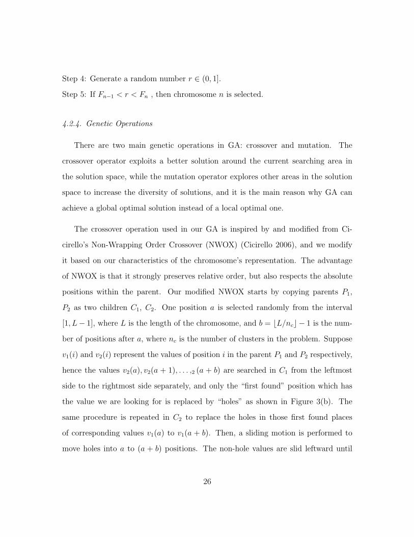
The crossover operation used in our GA is inspired by and modified from Ci-

cirello’s Non-Wrapping Order Crossover (NWOX) (Cicirello 2006), and we modify

it based on our characteristics of the chromosome’s representation. The advantage

of NWOX is that it strongly preserves relative order, but also respects the absolute

positions within the parent. Our modified NWOX starts by copying parents P1,

P2 as two children C1, C2. One position a is selected randomly from the interval

[1, L− 1], where L is the length of the chromosome, and b = bL/ncc − 1 is the num-

ber of positions after a, where nc is the number of clusters in the problem. Suppose

v1(i) and v2(i) represent the values of position i in the parent P1 and P2 respectively,

hence the values v2(a), v2(a + 1), . . . ,2 (a + b) are searched in C1 from the leftmost

side to the rightmost side separately, and only the “first found” position which has

the value we are looking for is replaced by “holes” as shown in Figure 3(b). The

same procedure is repeated in C2 to replace the holes in those first found places

of corresponding values v1(a) to v1(a + b). Then, a sliding motion is performed to

move holes into a to (a + b) positions. The non-hole values are slid leftward until

26

Figure 3: Steps of modified NWOX

all of them are grouped together contiguously. All remaining non-holes in the region

are slid rightward while leaving holes in the region (see Figure 3(c)). Then, values

v2(a), v2(a+ 1), . . . , v2(a+ b) of parent P2 are placed in position a, a+ 1, . . . , a+ b in

child C1, and, similarly, values v1(a), v1(a+ 1), . . . , v1(a+ b) of parent P1 are placed

in position a, a+ 1, . . . , a+ b in child C2 as Figure 3(d).

On the other hand, the mutation operator is performed based on “Insert mu-

tation”. The Insert mutation removes a value in the chromosome randomly, and

re-inserts that value into a randomly selected position. The mutation operation for

each child is executed based on a threshold probability value.

4.2.5. Feasibility Test and Enforced Mutation

In the GA employed in this study, one important mechanism is the feasibility test

which is used to test whether a child generated from genetic operations is feasible

or not. A child is considered to be feasible if all tours contained in this chromosome

are valid. In our case, a valid tour is one where any location will not be visited more

than once in a tour. In addition, based on Theorems 1 and 2, we can delete those

27

tours that have more than one cluster in common, or are k -split cycle tours. The

benefit of doing this is that we will not waste time testing some tours that are not

able to become the dominating solutions in the multi-objective optimization process

due to Theorems 1 and 2.

If one of the tours in the chromosome is invalid, enforced mutation is applied

to modify invalid tours. The idea of enforced mutation is to remove the location

that is visited multiple times or causes the violation of Theorems 1 and 2, and to

switch it with any other location in other tours without resulting in any invalidity.

The location to be switched with is chosen randomly. This operation is performed

repeatedly until all tours are valid.

4.2.6. Population Update

After the genetic operations, 2N chromosomes, including N parents and N chil-

dren respectively, are available. Because the size of the population is fixed, half of

these chromosomes will be eliminated due to their poor quality. For this purpose,

all children are evaluated to obtain fitness values and compared with parents. Then,

the best N chromosomes are chosen to be the population in the next generation.

Through the procedure described above, the final output of the tour generator is

a set of tours. Thus, the number of tours actually used in the mathematical model is

limited to an acceptable number, based on the preference of users. Meanwhile, the

model proposed above is expected to be more solvable than before.

28

4.3. Vehicle Assignment Heuristic

We also use a Vehicle Assignment Heuristic (VAH). The purpose of this approach

is to reduce the number of vehicles and also to reduce the number of tours used in the

model at the same time. The idea is to decompose the original problem into several

smaller subproblems in which each subproblem only contains a partial number of

vehicles in order to obtain solutions faster. After solving these subproblems, the

final solution for our problem will be constituted by combining all solutions from

them.

We first define some notation. Assume a set of vehicles V = 1, . . . , l is used to

deliver relief supplies to a set of clusters C = (ck, k = 1, . . . , j), and di(ck) represents

the demand of item i in cluster ck. If we use “it” to indicate the iteration of the

algorithm have been executed, I as the total desired number of iteration in the

algorithm, τ as the number of times that the solution is not improved after an

iteration, and TH as the maximum times allowed in a row that the solution is not

improved, then the VAH procedures can be described as follows.

VAH algorithm:

1. Randomly assign a partial number of vehicles v(gn) to serve only partial clusters

c(gn) (≤ 3 preferably), gn is the collection of n groups of vehicles and their

corresponding serving clusters, where∑

n v(gn) = l, and ∀p, q ∈ n, c(gp) ∩

c(gq) = φ.

2. For each gn, all feasible shortest travel time tours are determined.

3. For each gn, construct the mathematical model based on v(gn), c(gn), and the

corresponding demand di(ck), ∀i, ∀ck ∈ c(gn); solve n problems by CPLEX,

and get the objective values zn and the total objecitve value zall =∑

n zn. If

29

it is in the initial step, set the best total objective value z∗all = z0all, and it = 1.

4. Find a pair of groups (p, q) that has the minimum and maximum objective

value, respectively.

5. If v(gp) > 1,then do steps 6 and 7:

6. Remove one vehicle from v(gp), and assign it to v(gq).

7. Update zp,zq, and zall.

8. If zitall < z∗all, update z∗all = zit

all. Go to step 13.

9. Else z∗all = z∗all, and τ = τ + 1.

10. If τ < TH, go to step 5.

11. Else Stop the algorithm.

12. Else Find the next minimum objective value group, go to step 5.

13. If it < I, go to step 2.

14. Else Stop the algorithm.

5. Multi-Objective Optimization Methods

Several methods developed for multi-objective optimization in vehicle routing

problems have been proposed in the literature. They can be divided into three

categories: scalar methods, Pareto methods, and others (Jozefowiez et al. 2008).

Scalar methods use mathematical transformations to integrate multiple objectives.

Pareto methods are used often in evolutionary algorithms by applying the notion of

Pareto dominance to evaluate or compare objectives. The third category is methods

considering various objectives separately. Among them, scalar methods are still

frequently applied in multi-objective optimization problems. In general, the weighted

sum method and the ε-constraint method (Chankong and Haimes 1983) are two

30

major methods in scalar methods. In this paper, an up-to-date scalar method called

the elastic constraints method (Ehrgott 2006) is applied to present optimum results

of multi-objective optimization in our problem. In this section, we provide a brief

introduction to this method.

Suppose a multi-objective integer programming model is expressed as follows:

min Cx

s.t. x ∈ X

where C is a p × n objective function matrix with integer coefficients cki, k =

1, . . . , p; i = 1, . . . , n, and X = {x ∈ Zn : Ax = b, x ≥ 0}. We also denote that ck

as the kth row of C and yk = ckx as the kth objective value. Then, a feasible so-

lution x∗ is efficient if there is no x ∈ X such that Cx ≤ Cx∗, and y∗ = Cx∗ is

non-dominated if x∗ is efficient. For solving a multi-objective programming problem,

we are looking for the set of all efficient solutions x∗ and the set of non-dominated

points y∗.

In the ε-constraint method, one of the p objectives is retained in the objective,

and the other p−1 objectives become constraints. Therefore, the multiple objectives

become one as shown in equation (19) and p−1 new constraints are added in addition

to the original constraints x ∈ X in the problem. The formulation of the new

objective and the ε-constraints are:

min cjx

s.t. ckx ≤ εk, k 6= j

x ∈ X

(19)

31

All efficient solutions can be found by specifying the εk values. A nice property exists:

x∗ is efficient if and only if it is an optimal solution of (19) for all j = 1, . . . , p, where

εk = ckx, k 6= j (Ehrgott 2006). However, due to the fact that the upper bound

constraints ckx ≤ εk, k 6= j are knapsack-type constraints, the above property is

usually compromised due to the difficulty of solving (19).

Therefore, based on the ε-constraint method, the elastic constraints method was

proposed (Ehrgott 2006) aiming to combine the advantages of the weighted sum

method and the ε-constraint method but avoiding their disadvantages. In other

words, this method tries to solve a single objective version of the multi-objective

programming problem as the weighted sum method and is also able to generate all

efficient solutions as the ε-constraint method. As shown in equation (20), multiple

objective functions are converted to a single objective function with penalty terms,

and the elastic constraints are added as constraints.

min cjx+∑

k 6=j µksk

s.t. ckx+ Ik − sk = εk, k 6= j

sk, Ik ≥ 0, k 6= j

x ∈ X

(20)

where µk as the penalty coefficients, and εk is a specified value. Two additional

variables are used, slack variables Ik and surplus variables sk, to make the upper

bounds on constraints in (19) into equality constraints. In the above formulation,

two parameters are required to be determined, the penalty coefficients µk, and the

right-hand side values εk, which are usually decided by users.

32

6. Computational Results

In this section, the computational results are presented. Three parts are included

in the computational experiments. In the first part, a random instance generator is

designed to produce numerical instances for the following computational experiments.

In the second part, a comparison of performance among different approaches is pro-

vided to evaluate their advantages and disadvantages. In the last part, the tradeoff

analysis among three objective functions is conducted to present the dilemma of

decision making when facing a multiple objective scenario.

6.1. Random Instance Generator

The random instance generator has been coded in C. We assume the working

area of the disaster relief operation is in a 50 square mile area. The location of the

depot and all demand clusters are randomly located by the instance generator in

this area with the outputs of coordinate points. To transform Euclidean distances

to road distances, the following equation is adopted from the literature (Love and

Morris 1979):

d (q, r; k, p, s) = k

[2∑

i=1

|qi − ri|p]1/s

(21)

where q and r are coordinate points on the plane in the disaster area, and k, p, s

are parameters. Suggested ranges of these parameters are k ∈ {0.80, 2.29}, p, s ∈

{0.90, 2.29}, respectively. In our instance generator, parameters are randomly gen-

erated from corresponding ranges of each parameter. It is noted that only distances

between the depot and each cluster are estimated according to (21), and distances

among clusters are generated randomly based on the triangular inequality (i.e., road

33

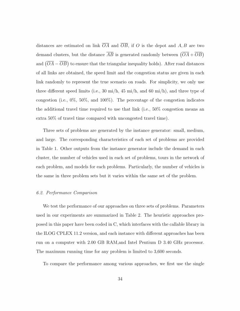
distances are estimated on link OA and OB, if O is the depot and A,B are two

demand clusters, but the distance AB is generated randomly between(OA+OB

)and

(OA−OB

)to ensure that the triangular inequality holds). After road distances

of all links are obtained, the speed limit and the congestion status are given in each

link randomly to represent the true scenario on roads. For simplicity, we only use

three different speed limits (i.e., 30 mi/h, 45 mi/h, and 60 mi/h), and three type of

congestion (i.e., 0%, 50%, and 100%). The percentage of the congestion indicates

the additional travel time required to use that link (i.e., 50% congestion means an

extra 50% of travel time compared with uncongested travel time).

Three sets of problems are generated by the instance generator: small, medium,

and large. The corresponding characteristics of each set of problems are provided

in Table 1. Other outputs from the instance generator include the demand in each

cluster, the number of vehicles used in each set of problems, tours in the network of

each problem, and models for each problems. Particularly, the number of vehicles is

the same in three problem sets but it varies within the same set of the problem.

6.2. Performance Comparison

We test the performance of our approaches on three sets of problems. Parameters

used in our experiments are summarized in Table 2. The heuristic approaches pro-

posed in this paper have been coded in C, which interfaces with the callable library in

the ILOG CPLEX 11.2 version, and each instance with different approaches has been

run on a computer with 2.00 GB RAM,and Intel Pentium D 3.40 GHz processor.

The maximum running time for any problem is limited to 3,600 seconds.

To compare the performance among various approaches, we first use the single

34

Table 1: Characteristics of Problem Sets

Set Problem No. of clusters No. of tours No. of vehicles1 3 9 202 3 9 18

Small 3 3 9 174 3 6 205 3 6 10

1 4 22 202 4 22 18

Medium 3 4 22 174 4 21 205 4 22 10

1 5 31 202 5 33 18

Large 3 5 31 174 5 39 205 5 41 10

Table 2: Summary of Parameters

Parameters SettingVehicle: capacity: 11580 kg

volume: 56 m3

Items:medicine ship. weight: 86.5 kg; ship. volume: 0.22 m3

water purificationsequipment ship. weight: 400 kg; ship. volume: 4.3 m3

canned food ship. weight: 700 kg; ship. volume: 1.3 m3

Working hours 12 hoursPlanning periods 4

35

objective problem to evaluate the performance. In our study, due to the scenario of

disaster relief operations, equation (1) is regarded as the most important objective

function that it aims to minimize unsatisfied demand. Table 3 summarizes results

from various approaches by solving the single objective problem with equation (1).

The first two columns identify the problem IDs and the number of tours used in

each problem. Under the CPLEX MIP column, the optimal objective value, the

running time (seconds), and the MIP gap is shown. For some problems, there is no

feasible solution available within 3,600 seconds, so we designate this as infeasible.

In addition, based on our preliminary experiments, our model is very difficult to

prove optimality by using the default setting (MIP gap = 0.001%) of CPLEX, so we

modify this parameter to 0.01% to reduce the required time of proving optimality.

Under the tour generation column, the same data is provided as under the CPLEX

MIP column. It is noted that the number of tours used in M1-M5 and L1-L5 is

10 respectively, which is the result from the tour generation approach described in

section 4.2. Under the VAH approach, the solution is presented as a pecentage of

the optimal value, and the running time is also reported in the last column.

Table 4 summarizes the average performance of both the Tour Generation ap-

proach and VAH approach. The Tour Generation approach fixes the infeasible situ-

ation in CPLEX MIP, and the average running time is also reduced by about 22.3%.

The average percentage of optimality is 99.8% which is almost the same as CPLEX

MIP. However, the variance of running times in the Tour Generation approach is

still high (i.e., from 17.81 to 3,600 seconds), because CPLEX spends a long time

in proving optimality. Figure 4 reveals this situation by showing the relationship

of the running time and corresponding solutions for some instances (i.e, for these

four instances, they all reach or almost reach the final optimal solution in about 600

36

Tab

le3:

Per

form

ance

Tab

le

Pro

b.

CP

LE

XM

IPT

our

Gen

erat

ion

VA

HID

Ob

j.T

ime

MIP

gap

Ob

j.T

ime

MIP

gap

%op

tim

alit

yT

ime

valu

e(s

econ

ds)

(%)

valu

e(s

econ

ds)

(%)

(sec

onds)

S1

232

178.

110.

0223

217

8.11

0.02

99.8

817

S2

344

44.5

40.

0334

444

.54

0.03

99.8

552

S3

11,7

9231

2.16

0.07

11,7

9231

2.16

0.07

98.2

118

S4

49,4

2426

0.15

0.10

49,4

2426

0.15

0.10

98.6

414

S5

35,8

8417

.81

0.07

35,8

8417

.81

0.07

91.9

35

M1

48,3

843,

600

0.12

47,5

0018

7.75

0.07

98.0

879

M2

infe

asib

len/a

n/a

16,7

883,

600

0.12

99.3

442

M3

41,5

003,

287.

170.

0741

,100

311.

60.

0798

.25

42M

4in

feas

ible

n/a

n/a

68,6

8081

0.94

0.10

99.6

039

M5

36,3

6822

77.2

10.

1036

,708

3,60

00.

1197

.92

15

L1

infe

asib

len/a

n/a

74,0

113,

600

0.10

92.1

815

L2

infe

asib

len/a

n/a

39,4

723,

600

0.14

96.8

322

L3

164,

449

3,60

01.

4316

3,24

93,

600

1.43

85.1

345

L4

infe

asib

len/a

n/a

83,9

363,

600

0.11

96.6

466

L5

422,

855

3,60

01.

5342

2,85

53,

600

0.43

80.0

814

37

seconds). On the other hand, the VAH approach finds a solution in a very short

running time with a 4.5% optimality gap. Although the solution is less optimal than

the other two approaches, we concluded that VAH can be an efficient approach in a

disaster relief operation due to the special requirement of quick responses.

Figure 4: Instances showing relationship between % optimality gap and running time

Table 4: Average Performance Results

CPLEX MIP Tour Generation VAHAverage time Average time Average Average time Average(seconds) (seconds) % optimality (second) % optimality2,345.14 1,821.54 99.8 32.33 95.5

38

6.3. Tradeoff Analysis among Objectives

In this section, we present the tradeoff analysis among three objectives in our

logistic model. We use problem M2 to present the analysis in this section. The

relationship between objective functions 1, 2, and 3 is shown in Figures 5 and 6,

where objective 1 aims to minimize unsatisfied demand, objective 2 intends to min-

imize total travel time for all tours and vehicles and objective 3 means to minimize

the difference in satisfaction rate between clusters which have the highest and the

lowest ones. They are obtained by using the elastic constraint method. For both

figures, the x -axis represents ε1, which is the tolerable increment of the penalty cost

due to unsatisfied demand, and the y-axis represents the travel cost and maximum

satisfaction rate, respectively. In our experiment,the tolerable increments are defined

from 1% to 9%, and therefore, ε1 is computed by the equation ε1 = Z∗1(1 + δ), where

δ = 0.01, . . . , 0.09. For both figures, the line represents the approximate Pareto front

of the two objectives when we fix the other third objective (i.e, the objective 3 is

fixed in Figure 5). As the penalty cost increases, both the travel cost and the maxi-

mum satisfaction rate is reduced respectively. Therefore, it is obvious that there are

tradeoff situations for users to determine what increments of the penatly cost are

desired. In particular, the impact of increasing the allowable penalty cost for the

objective 3 is more sensitive to that for the objective 2 since the objective value of

the objective 3 almost reaches zero when we increase the penalty cost by 4%.

Moreover, if all three objectives are considered at the same time, Figure 7 shows

the approximate Pareto front surface by the elastic constraint method with param-

eters u2 and u3 equal 100 for the problem M1. We use values of objectives 2 and

3 from Figures 5 and 6 to investigate the impact of both objectives to the penalty

39

Figure 5: Pareto front of objective 1 and 2

Figure 6: Pareto front of objective 1 and 3

40

cost. From the figure, the maximum difference of satisfaction rates does not affect

too much penalty cost under the same level of travel costs, while the penalty cost is

significant influenced by the travel cost. The travel cost between 780.3 to 816.3 is

the ideal targeted range to pursue since it results in a near-optimal penalty cost but

at the same time significantly reduces the travel cost.

Figure 7: Pareto Front Surface

7. Conclusions and Future Work

This paper proposes a logistics model in a disaster relief operation for deliv-

ery of critical items. Our model considers a multi-objective, multi-period, multi-

commodity, and multi-vehicle scenario. The distinguishing feature of our work is

to consider the delivery priorities of different items and to encompass this idea in

41

one of our objecitves. In addition, we also determine two main factors that increase

difficulties of solving this problem: the number of tours and the number of vehicles.

Two heuristic approaches are developed, the Tour Generation heuristic and the Ve-

hicle Assignment heuristic (VAH), to overcome these two factors. The performance

of these two approaches is analyzed and their efficiency is investigated. We found

that, in general, the Tour Generation heuristic can resolve infeasible situations effec-

tively, and provide good solutions. On the other hand, the VAH approach provides

solutions in a short computational time while they have about 5% optimality gap

compared to solutions from the Tour Generation heuristic. Furthermore, the tradeoff

analysis of a multi-objective optimization is provided. We investigate relationships

among the three objectives, and determine the targeted range of the travel cost that

is worth pursuing without significantly increasing the penalty cost.

We suggest three directions for future work. The first is to investigate the robust-

ness of our model with respect to uncertainty in demand values, congestion levels,

network accessibility, and cluster correlations with respect to the highway roadways.

The second is to develop more efficient multi-objective optimization methodologies

for our problem. The third is to consider a distributed scenario in which several

temporary depots are required to be located and serve as “bridges” between the

distribution center and demand locations.

References

Archetti, C., Mansini, R., Speranza, M. G., 2005. Complexity and reducibility of the skip

delivery problem. Transportation Science 39 (2), 182–187.

42

Archetti, C., Savelsbergh, M. W. P., Speranza, M. G., 2006a. Worst-case analysis for split

delivery vehicle routing problems. Transportation Science 40 (2), 226–234.

Archetti, C., Savelsbergh, M. W. P., Speranza, M. G., 2008. To split or not to split: That is

the question. Transportation Research Part E: Logistics and Transportation Review

44 (1), 114–123.

Archetti, C., Speranza, M. G., Hertz, A., 2006b. A tabu search algorithm for the split

delivery vehicle routing problem. Transportation Science 40 (1), 64–73.

Baker, B. M., Ayechew, M. A., 2003. A genetic algorithm for the vehicle routing problem.

Computers and Operations Research 30 (5), 787–800.

Balcik, B., Beamon, B. M., Smilowitz, K., 2008. Last mile distribution in humanitarian

relief. Journal of Intelligent Transportation Systems: Technology, Planning, and Op-

erations 12 (2), 51–63.

Barbarosoglu, G., Ozdamar, L., Cevik, A., 2002. An interactive approach for hierarchi-

cal analysis of helicopter logistics in disaster relief operations. European Journal of

Operational Research 140 (1), 118–133.

Belenguer, J. M., Martinez, M. C., Mota, E., 2000. A lower bound for the split delivery

vehicle routing problem. Operations Research 48 (5), 801–810.

Bompadre, A., Dror, M., Orlin, J. B., 2006. Improved bounds for vehicle routing solutions.

Discrete Optimization 3 (4), 299–316.

Chankong, V., Haimes, Y., 1983. Multiobjective Decision Making Theory and Methodology.

Elsevier Science, New York.

Chuah, K. H., Jon, C. Y., 2005. Routing for a just-in-time supply pickup and delivery

system. Transportation Science 39 (3), 328–339.

Cicirello, V. A., 2006. Non-wrapping order crossover: An order preserving crossover oper-

ator that respects absolute position. GECCO’ 06: Genetic and Evolutionary Compu-

tation Conference, 1125–1131.

43

Dror, M., Laporte, G., Trudeau, P., 1994. Vehicle-routing with split deliveries. Discrete

Applied Mathematics 50 (3), 239–254.

Dror, M., Trudeau, P., 1989. Savings by split delivery routing. Transportation Science

23 (2), 141–145.

Dror, M., Trudeau, P., 1990. Split delivery routing. Naval Research Logistics 37, 383–402.

Ehrgott, M., 2006. A discussion of scalarization techniques for multiple objective integer

programming. Annals of Operations Research 147 (1), 343–360.

Fiedrich, F., Gehbauer, F., Rickers, U., 2000. Optimized resource allocation for emergency

response after earthquake disasters. Safety Science 35, 41–57.

Frizzell, P. W., Giffin, J. W., 1992. The bounded split delivery vehicle-routing proble with

grid network distances. Asia-Pacific Journal of Operational Research 9 (1), 101–116.

Frizzell, P. W., Giffin, J. W., 1995. The split delivery vehicle scheduling problem with time

windows and grid network distances. Computers and Operations Research 22 (6),

655–667.

Goldberg, D., 1989. Genetic Algorithms in Search, Optimization and Machine Learning.

Addison-Wesley, New York.

Gong, Q., Batta, R., 2007. Allocation and reallocation of ambulances to casualty clusters

in a disaster relief operation. IIE Transactions 39 (1), 27–39.

Ho, S. C., Haugland, D., 2004. A tabu search heuristic for the vehicle routing problem

with time windows and split deliveries. Computers and Operations Research 31 (12),

1947–1964.

Ho, W., Ho, G. T. S., Ji, P., Lau, H. C. W., 2008. A hybrid genetic algorithm for the

multi-depot vehicle routing problem. Engineering Applications of Artificial Intelli-

gence 21 (4), 548–557.

Jin, M. Z., Liu, K., Bowden, R. O., 2007. A two-stage algorithm with valid inequalities

44

for the split delivery vehicle routing problem. International Journal of Production

Economics 105 (1), 228–242.

Jin, M. Z., Liu, K., Eksioglu, B., 2008. A column generation approach for the split delivery

vehicle routing problem. Operations Research Letters 36 (2), 265–270.

Jotshi, A., Gong, Q., Batta, R., 2009. Dispatching and routing of emergency vehicles in

disaster mitigation using data fusion. Socio-Economic Planning Sciences 43 (1), 1–24.

Jozefowiez, N., Semet, F., Talbi, E.-G., 2008. Multi-objective vehicle routing problems.

European Journal of Operational Research 189 (2), 293–309.

Love, R. F., Morris, J. G., 1979. Mathematical models of road travel distances. Management

Science 25 (2), 130–139.

Nowak, M., Ergun, O., White, C. C., 2008. Pickup and delivery with split loads. Trans-

portation Science 42 (1), 32–43.

Ohlmann, J. W., Fry, M. J., Thomas, B. W., 2008. Route design for lean production

systems. Transportation Science 42 (3), 352–370.

Ozdamar, L., Ekinci, E., Kucukyazici, B., 2004. Emergency logistics planning in natural

disasters. Annals of Operations Research 129 (1-4), 217–245.

Prins, C., 2004. A simple and effective evolutionary algorithm for the vehicle routing prob-

lem. Computers and Operations Research 31 (12), 1985–2002.

Sheu, J.-B., 2007. An emergency logistics distribution approach for quick response to urgent

relief demand in disasters. Transportation Research Part E: Logistics and Transporta-

tion Review 43 (6), 687–709.

Silva, C. A., Sousa, J. M. C., Runkler, T. A., 2008. Rescheduling and optimization of

logistic processes using ga and aco. Engineering Applications of Artificial Intelligence

21 (3), 343–352.

Yi, W., Kumar, A., 2007. Ant colony optimization for disaster relief operations. Trans-

portation Research Part E: Logistics and Transportation Review 43 (6), 660–672.

45

Yi, W., Odamar, L., 2007. A dynamic logistics coordination model for evacuation and

support in disaster response activities. European Journal of Operational Research

179 (3), 1177–1193.

46