A logic toolbox for modelingknowledge and information inmulti-agent systems and social

epistemology

by

Jens Ulrik Hansen

A dissertation presented to the facultiesof Roskilde University in partial fulfillment of

the requirement for the PhD degree

Department of Communication, Business and Information Technologies /

Department of Culture and Identity

Roskilde University, Denmark

September 2011

ii

Abstract

This dissertation consists of a collection of papers on pure and applied modal

logics preceded by an introduction that ties them together. The papers and the

variety of topics discussed in them can be viewed as a contribution to a logic

toolbox. More specifically, a logic toolbox streamlined to model information,

knowledge, and beliefs. The logic tools have many applications in various fields

such as computer science, philosophy, mathematics, linguistics, economics, and

other social sciences, but in this thesis the focus will be on their application

in social epistemology and multi-agent systems.

After the introduction, which outlines the logic toolbox and some of its ap-

plications, follow four technical chapters that expand the logic toolbox (chap-

ters 2, 3, 4, and 5) and two chapters that show the logic tools at work (chapters

6 and 7). In Chapter 2 a many-valued hybrid logic is introduced and a sound,

complete, and terminating tableau system is given. Chapter 3 is a supplement

to Chapter 2 and discusses various alternative definitions of the semantics of

the hybrid part of the many-valued hybrid logic. Chapter 4 combines public

announcement logic with hybrid logic and gives a sound and complete axioma-

tisation of the logic as well as discussing extensions with other modalities such

as distributed knowledge. In Chapter 5, terminating tableau systems using

reduction axioms as rules are given for standard dynamic epistemic logic as

well as the hybrid public announcement logic of Chapter 4. Chapter 6 uses

a dynamic epistemic logic to model the phenomenon of pluralistic ignorance.

Finally, Chapter 7 uses first-order logic and description logic to discuss founda-

tional issues in knowledge representation of regulatory relations in biomedical

pathways.

This dissertation makes numerous contributions to the field of which the

following three are the most important:

• A detailed investigation of the combination of hybrid logic and pub-

lic announcement logic, showing in particular that the proof theoretic

advantages of hybrid logic (such as automatic completeness with pure

iii

formulas) extend to hybrid public announcement logic (chapters 4 and

5).

• An approach to constructing terminating tableau systems for hybrid log-

ics is shown to be extremely general in the sense that it extends to both

many-valued hybrid logic (Chapter 2), dynamic epistemic logic, and hy-

brid public announcement logic (Chapter 5).

• This dissertation touches upon the issue of how knowledge and beliefs

of a group of agents relate to the knowledge and beliefs of the individ-

uals of the group. How knowledge or beliefs of the individual agents

can be aggregated to yield group knowledge or group beliefs is studied

in Section 1.3.3 of the introduction, and how information and beliefs

flow among a group of agents involved in the phenomenon of pluralistic

ignorance is studied in Chapter 6.

iv

Resume

Denne afhandling bestar af en samling artikler, der omhandler teoretisk og an-

vendt modallogik, bundet sammen af en forudgaende indledning. Artiklerne

og de deri behandlede emner kan ses som et bidrag til en logik-værktøjskasse.

Mere præcist: en logik-værktøjskasse trimmet til at modellere information,

viden og formodninger. Logik-værktøjet har mange anvendelser i discipliner

sasom datalogi, filosofi, matematik, lingvistik, økonomi og andre samfundsv-

idenskaber, men i denne afhandling er fokusset paanvendelser i social episte-

mologi og multi-agent systemer.

Efter introduktionen, der skitserer logik-værktøjskassen og nogle af dens

anvendelser, følger fire tekniske kapitler, som udvider denne værktøjskasse

(kapitlerne 2, 3, 4 og 5) og to kapitler, der viser logik-værktøjerne i arbejde

(kapitlerne 6 og 7). I kapitel 2 introduceres en mange-værdi hybridlogik og

et sundt, fuldstændigt og terminerende tableau-system given for den. Kapitel

3 er et tillæg til kapitel 2 og diskuterer forskellige alternative definitioner af

semantikken for den hybride del af mange-værdi hybridlogikken. Kapitel 4

kombinerer “offentlig annoncerings”-logik med hybridlogik, indfører en sund

og fuldstændig aksiomatisering af logikken og diskuterer desuden udvidelser

med andre modaliteter sasom distribueret viden. I kapitel 5 præsenteres ter-

minerende tableau-systemer, hvor reduktionsaksiomer bruges som regler for

standard dynamisk epistemisk logik og den offentlig annoncerings-logik fra

kapitel 4. Kapitel 6 bruger en dynamisk epistemisk logik til at modellere

fænomenet “pluralistisk ignorance”. Endelig bruger kapitel 7 førsteordens-

logik og beskrivelseslogik til at diskutere fundamentet for vidensrepræsenta-

tion af regulatoriske relationer i biomedicinske netværk.

Afhandlingen kommer med adskillige videnskabelige bidrag. De tre vigtig-

ste er dog som følger:

• En detaljeret undersøgelse af kombinationen af hybridlogik og offentlig

annoncerings-logik, som særligt paviser, at de bevisteoretiske fordele ved

hybridlogik (sasom automatisk fuldstændighed med rene former) kan

v

overføres til hybrid offentlig annoncerings-logik (kapitlerne 4 og 5).

• En metode til at konstruere terminerende tableau-systemer for hybrid-

logik vises at være ekstrem generel i den forstand, at den kan udvides til

bade mange-værdi hybridlogik (kapitel 2) og dynamisk epistemisk logik

og offentlig annoncerings-logik (kapitel 5).

• Endelig berører denne afhandling emnet, om hvordan en gruppes vi-

den og formodninger relaterer sig til gruppens individers viden og for-

modninger. Hvordan individuelle agenters viden eller formodninger kan

aggregeres til gruppeviden eller gruppeformodninger diskuteres i afsnit

1.3.3 af introduktionen. Hvordan information og formodninger flyder

mellem en gruppe af agenter involveret i fænomenet pluralistisk igno-

rance udforskes i kapitel 6.

vi

Acknowledgments

In the process of writing this dissertation and conducting the research it re-

ports, I have received support and advice from a great number of people. At

the end of each chapter, the people who have specifically influenced the partic-

ular research in that chapter are acknowledged. In addition, however, I would

like to take this opportunity to give a general thanks to a number of people.

First of all, I would like to thank my supervisors Torben Brauner and Stig

Andur Pedersen for giving me the opportunity to write this PhD dissertation,

for inspiring discussions, for encouraging my work, and for providing useful

comments on my papers.

I would also like to thank the members of my assessment committee, John

Gallagher, Wiebe van der Hoek, and Barteld Kooi for accepting to evaluate

my thesis and providing numerous insightful comments and suggestion.

The papers that constitute chapter 2 and 7 are co-authored with Torben

Brauner and Thomas Bolander respectively Sine Zambach. I would like to

thank them for exceptionally enjoyable and fruitful collaborations - working

together is always more fun than working alone! Thomas Bolander deserves

special thanks for many inspiring discussions, for introducing me to the logic

community in Denmark, and for always providing plenty of academic and

career advice. Also thank you to Valentin Goranko and the rest of the DTU-

people, with whom I have had many inspiring discussions.

Thank you to Henriette for proofreading parts of this dissertation.

During my PhD studies I also had the chance to spend one year at the

Institute of Logic, Language and Computation at the University of Amsterdam

and in this connection I have many people to thank. First of all, Frank Veltman

for being my official host at the ILLC. Secondly, the teachers, organizers, and

participants of the many courses, seminars, workshops, conference, and study

groups I attended in Amsterdam. Finally, a thanks goes out to the many

people who made my stay in Amsterdam an exceptionally enjoyable experience

vii

- again, mentioning you all would be exceedingly difficult.

Besides of Amsterdam, I have attended many conferences, workshops, and

summer schools, where I met numerous interesting people and had count-

less inspiring discussions. Especially the European Summer School in Logic,

Language and Information (ESSLLI) has introduced me to many interesting

people and taught me a great deal. Thanks to Vincent Hendricks for bring-

ing ESSLLI to Copenhagen last year, and thanks to the other organizers and

student session co-chairs for making it a great experience. Also, thanks to the

organizers of the PhDs in Logic workshops, which I much enjoyed as well.

In general, throughout the past three and a half years I have benefitted

from the discussions with various academic colleagues and friends. There

are too many to list and any attempt to make a list would most likely be

insufficient.

My colleagues, both at the Philosophy and at the Computer Science de-

partment at Roskilde University, also deserve a big thank you for creating a

most pleasant working environment – especially my fellow PhD students (or

postdoc) and friends Christian, Mai, Matthieu, Ole, and Sine. I cannot imag-

ine how I would have completed my PhD studies without Ole and Sine being

there.

Finally, I would like to thank all of my family (especially my parents and

my brother) and friends for putting up with me the past three and a half years.

For that I am deeply grateful. Finally, thanks to Kristine for being who she

is.

Jens Ulrik Hansen

Copenhagen, September 2011

viii

Contents

Abstract iii

Resume v

Acknowledgments vii

1 Introduction 1

1.1 The logic toolbox I: Modal logic and some of its friends . . . . 2

1.1.1 Modal logic . . . . . . . . . . . . . . . . . . . . . . . . . 3

1.1.2 Hybrid logic . . . . . . . . . . . . . . . . . . . . . . . . . 6

1.1.3 Description logic . . . . . . . . . . . . . . . . . . . . . . 10

1.1.4 Epistemic logic . . . . . . . . . . . . . . . . . . . . . . . 13

1.1.5 Dynamic epistemic logic . . . . . . . . . . . . . . . . . . 16

1.1.6 Many-valued logics . . . . . . . . . . . . . . . . . . . . . 22

1.2 The logic toolbox II: Proof theory . . . . . . . . . . . . . . . . 24

1.2.1 The proof theory of modal logic . . . . . . . . . . . . . . 24

1.2.2 The proof theory of hybrid logic . . . . . . . . . . . . . 33

1.2.3 The proof theory of dynamic epistemic logic . . . . . . . 39

1.3 The toolbox at work: modeling information, knowledge, and

beliefs . . . . . . . . . . . . . . . . . . . . . . . . . . . . . . . . 43

1.3.1 Information, knowledge, and beliefs in philosophy and

computer science . . . . . . . . . . . . . . . . . . . . . . 43

1.3.2 Logic-based modeling of information, knowledge, and

beliefs . . . . . . . . . . . . . . . . . . . . . . . . . . . . 51

1.3.3 Judgment aggregation and many-valued logics . . . . . 62

1.4 Outline of the thesis . . . . . . . . . . . . . . . . . . . . . . . . 70

2 Many-Valued Hybrid Logic 71

2.1 Introduction . . . . . . . . . . . . . . . . . . . . . . . . . . . . . 71

ix

CONTENTS

2.2 A Many-Valued Hybrid Logic language . . . . . . . . . . . . . . 73

2.2.1 Syntax for MVHL . . . . . . . . . . . . . . . . . . . . . 73

2.2.2 Semantics for MVHL . . . . . . . . . . . . . . . . . . . 74

2.2.3 The relation to intuitionistic hybrid logic . . . . . . . . 75

2.3 A tableau calculus for MVHL . . . . . . . . . . . . . . . . . . . 78

2.4 Termination . . . . . . . . . . . . . . . . . . . . . . . . . . . . . 83

2.5 Completeness of the basic calculus . . . . . . . . . . . . . . . . 87

3 Alternative semantics for a many-valued hybrid logic 97

3.1 MVHL1 . . . . . . . . . . . . . . . . . . . . . . . . . . . . . . 99

3.2 MVHL2 . . . . . . . . . . . . . . . . . . . . . . . . . . . . . . 102

3.3 MVHL3 . . . . . . . . . . . . . . . . . . . . . . . . . . . . . . 104

3.4 MVHL4 . . . . . . . . . . . . . . . . . . . . . . . . . . . . . . 107

3.5 MVHL5 . . . . . . . . . . . . . . . . . . . . . . . . . . . . . . 109

3.6 Still more logics! . . . . . . . . . . . . . . . . . . . . . . . . . . 112

3.7 Concluding remarks and further research . . . . . . . . . . . . . 112

4 A Hybrid Public Announcement Logic with Distributed Knowl-

edge 115

4.1 Introduction . . . . . . . . . . . . . . . . . . . . . . . . . . . . . 116

4.2 A hybrid logic with partial denoting nominals . . . . . . . . . . 118

4.2.1 Syntax and semantics . . . . . . . . . . . . . . . . . . . 119

4.2.2 Complete proof systems . . . . . . . . . . . . . . . . . . 121

4.3 Hybrid Public Announcement Logic . . . . . . . . . . . . . . . 129

4.4 Adding distributed knowledge and other modalities . . . . . . . 134

4.4.1 Adding distributed knowledge the standard way . . . . 135

4.4.2 Adding distributed knowledge directly . . . . . . . . . . 137

4.4.3 The definability of distributed knowledge using satisfac-

tion operators and the downarrow binder . . . . . . . . 138

4.4.4 A general way of adding modalities to public announce-

ment logic . . . . . . . . . . . . . . . . . . . . . . . . . . 139

4.4.5 A note on common knowledge . . . . . . . . . . . . . . . 143

4.5 Conclusion and further work . . . . . . . . . . . . . . . . . . . 143

4.6 Appendix: Alternative semantics for the public announcement

operator . . . . . . . . . . . . . . . . . . . . . . . . . . . . . . . 145

5 Terminating tableaux for dynamic epistemic logics 147

5.1 Introduction . . . . . . . . . . . . . . . . . . . . . . . . . . . . . 148

5.2 Dynamic epistemic logic . . . . . . . . . . . . . . . . . . . . . . 150

x

CONTENTS

5.3 A tableaux system for AM . . . . . . . . . . . . . . . . . . . . 156

5.3.1 Termination of the tableau system . . . . . . . . . . . . 157

5.3.2 Soundness and completeness of the tableau system . . . 161

5.4 A tableau for hybrid public announcement logic . . . . . . . . . 161

5.4.1 Termination of HPA tableaux . . . . . . . . . . . . . . 163

5.4.2 Soundness and completeness of the tableau system for

HPA . . . . . . . . . . . . . . . . . . . . . . . . . . . . 164

5.5 Concluding remarks and further research . . . . . . . . . . . . . 165

6 A Logic-Based Approach to Pluralistic Ignorance 167

6.1 Introduction . . . . . . . . . . . . . . . . . . . . . . . . . . . . . 167

6.2 Examples of pluralistic ignorance . . . . . . . . . . . . . . . . . 169

6.3 Plausibility models: A logical model of belief, knowledge, doubt,

and ignorance . . . . . . . . . . . . . . . . . . . . . . . . . . . . 170

6.4 Modeling pluralistic ignorance . . . . . . . . . . . . . . . . . . . 173

6.4.1 Formalizations and consistency of pluralistic ignorance . 173

6.4.2 The fragility of pluralistic ignorance . . . . . . . . . . . 176

6.5 Further research on logic and pluralistic ignorance . . . . . . . 180

6.5.1 Informational Cascades: How pluralistic ignorance comes

about and how it vanishes . . . . . . . . . . . . . . . . . 180

6.5.2 Private versus public beliefs – the need for new notions

of group beliefs . . . . . . . . . . . . . . . . . . . . . . . 181

6.5.3 How agents act . . . . . . . . . . . . . . . . . . . . . . . 181

6.6 Conclusion . . . . . . . . . . . . . . . . . . . . . . . . . . . . . 182

7 Logical Knowledge Representation of Regulatory Relations in

Biomedical Pathways 183

7.1 Introduction . . . . . . . . . . . . . . . . . . . . . . . . . . . . . 184

7.2 Related work and examples . . . . . . . . . . . . . . . . . . . . 185

7.2.1 Related work . . . . . . . . . . . . . . . . . . . . . . . . 185

7.2.2 Examples of regulation . . . . . . . . . . . . . . . . . . . 186

7.3 Ontological clarifications . . . . . . . . . . . . . . . . . . . . . 187

7.3.1 Research practice and granularity . . . . . . . . . . . . . 188

7.3.2 Underlying ontological assumptions - Instances and classes188

7.4 Analysis of the formal semantic . . . . . . . . . . . . . . . . . 189

7.4.1 A Logic formalization of regulatory relations . . . . . . 189

7.4.2 The relata of regulatory relations . . . . . . . . . . . . . 190

xi

CONTENTS

7.4.3 Modal, temporal and spatial aspect of regulatory rela-

tions . . . . . . . . . . . . . . . . . . . . . . . . . . . . 192

7.4.4 Description Logic representation of class relations . . . . 193

7.5 Discussion . . . . . . . . . . . . . . . . . . . . . . . . . . . . . 194

7.5.1 Applications in the biomedical domain . . . . . . . . . . 194

7.5.2 Future work . . . . . . . . . . . . . . . . . . . . . . . . . 198

8 Conclusion 201

Bibliography 221

xii

Chapter 1

Introduction

This thesis consists of a collection of papers on pure and applied logic that

covers a variety of technical results as well as a few applications. The primary

focus of the thesis is on technical issues invovled in expanding the logics and

their proof theory. There are a number of topics, methods, and ideas that are

shared by the papers and the aim of this introduction is to show how they can

all be viewed as part of a single project, namely the project of expanding the

logic toolbox for modeling knowledge and information in multi-agent systems

and social epistemology. This endeavor not only presupposes a certain view

of what logic is and can be used for, but also a certain view on what knowl-

edge and information are, and how agents, be it humans, computer programs,

or robots, represent, process, and reason about knowledge and information.

Therefore, this introduction is intended to clarify the view of knowledge and

information adopted in this endeavor, to clarify how this view results in ap-

plications within computer science and philosophy, and finally to clarify the

logical frameworks on which this thesis is based.

This introduction starts the unlocking of the toolbox by introducing the

logics appearing in this thesis, which include modal logic, hybrid logic, descrip-

tion logic, epistemic logic, dynamic epistemic logic, and many-valued logic.

The unlocking continues with a discussion of the proof theory of several of

these logics. Following the listing of the tools, the fields in which they can

be applied are outlined. This outline includes an introduction to information,

knowledge, beliefs and the problems they raise within areas of philosophy and

computer science as well as a discussion of how logic can be of assistance.1

1A word of warning for the computer scientist regarding the toolbox metaphor: The aim

of this thesis has been to develop a conceptual toolbox, not actual tools in form of computer

systems or programs.

1

Ch. 1. Introduction

1.1 The logic toolbox I: Modal logic and some of its

friends

Logic is an old subject within philosophy and has traditionally been defined as

the systematic study of valid reasoning. The central object of study was argu-

ments and their logical forms, based on which a notion of what constitutes a

valid argument could be properly defined: an argument being valid if the truth

of the premises ensures the truth of the conclusion. However, since the great

influence of computer science on logic, both as providing applications and new

theoretical concepts, the subject has become much broader. In general, there

is no doubt that logic has become a broader field due to its many applica-

tions within fields such as computer science, artificial intelligence, linguistics,

economics, and mathematics.

There is much that can be said about the history of logic, and the debate

of what constitutes the subject today is no trivial discussion either. Instead of

going further into these matters, an explanation of the view of logic adopted in

this thesis will be laid out. Here logic will be viewed simply as a modeling tool

and not as merely a study of arguments’ forms and notions of validity. Logic

can be viewed as just another formal/mathematical framework which can be

used to model various phenomena, such as computations, natural language, or

rational interactions.2 The view that logic is a formal tool, useful for modeling

various scenarios, is not claimed to be the only ideal view of logic, but it fits

very well with the current state of formal and social epistemology as well as

multi-agent systems and artificial intelligence. Within these fields logic can

provide a useful toolbox that certainly justifies further study.

However, this thesis just touches upon a corner of this enormous tool-

box. Nevertheless, all chapters of this thesis involve some kind of modal logic

(Chapter 7 only briefly). Therefore, modal logic, and some of its extensions,

will be discussed specifically in the rest of this section. In the discussion, focus

will be on the semantic aspects of the logics, but in Section 1.2 the syntactic

or proof theoretic aspects of some of the logics will be elaborated.

2Viewing logic as a modeling tool immediately raises two questions: What are we trying

to model and how adequate is the modeling? The main focus of this thesis is on the technical

issues involved in expanding existing tools and thus the adequateness of the logics developed

will be given very little attention. Examples of what logic in general can be used to model

is given Section 1.3. The chapters 6 and 7 are also examples of what logic can be used

to model, and the adequateness of the particular logics will be discussed in these chapters,

especially in Chapter 7.

2

1.1 The logic toolbox I: Modal logic and some of its friends

1.1.1 Modal logic

The beginning of modal logic is attributed to Aristotle [34] and ever since

then, modal logic has been a part of philosophy. Traditionally conceived,

modal logic is the study of reasoning with modal expressions such as “neces-

sarily”, “possibly”, “must”, “can” etc., which all moderate the truth values

of statements. Statements might not only be true they may be true with dif-

ferent modes, for instance necessarily true, possibly true etc.. More broadly

conceived modal logic also deals with other modalities than “it is necessary

that” and “it is possible that” (alethic modalities), for instance “it will be the

case that”, “it has always been the case that” (temporal modalities), “it is

obligatory that”, “it is permitted that” (deontic modalities) “a knows that”,

“a doubts that”, “a believes that” (epistemic and doxastic modalities). Modal

logic as the study of reasoning with such modal expressions is more or less the

standard view on what modal logic is within philosophy [64, 72, 131, 68].

However, modal logic has moved past the borders of philosophy and is now

broadly used within computer science, artificial intelligence, linguistics, math-

ematics, economic game theory and other fields. For instance, new modalities

have come in from computer science such as “after all runs of the program a”,

“once process a is started, eventually”. Furthermore, a mathematical gener-

alization of modal logic has also occurred: one of the standard references on

modal logic, [27], describes modal logic as a logic for reasoning about general

relational structures from an internal, local perspective. Moreover, [27] notes

that other logics can be used to reason about relational structures and modal

logic can reason about other things than relational structures, which leads to

two ways of extending the field of modal logic even further: New logics to

reason about relational structures can be developed and existing modal logics

can be used to reason about other kind of mathematical structures. Where

the view from philosophy of modal logic starts from modal expressions ap-

pearing in natural or formal languages, the view of modal logic as reasoning

about relational structures focuses on how modalities and their semantics are

defined mathematically, and therefore becomes a purely mathematical study.

All this goes to show that modal logic is a wide subject that appears in

several fields and lends itself to many different approaches. The broadness of

the subject is also witnessed by the recent handbook of modal logic [31]. In

conclusion, modal logic is one of the fastest growing corners of the logic tool-

box, both because of technical advances in the mathematical/computational

theory of modal logic and because of the many new applications within nu-

3

Ch. 1. Introduction

merous other fields. In the remainder of this section, standard modal logic

will be described in more detail. After introducing modal logic broadly, hy-

brid logic will be introduced in Section 1.1.2, description logic in Section 1.1.3,

epistemic logic in Section 1.1.4, dynamic epistemic logic in Section 1.1.5, and

many-valued logic in Section 1.1.6.

Viewing modal logic as a logic to reason about relational structures is an idea

that has had significant influence on modern modal logic. Using relational

structures to interpret the statements of modal logic is an idea going back to

the middle of the last century and is usually ascribed to Saul Kripke, even

though others had similar ideas at the time. However, Kripke’s formulation

remains the most general and clear, which is why the relational semantics is

often referred to as Kripke semantics. In the following it will either be referred

to as Kripke semantics or possible worlds semantics. For more on the early

development of the semantics of Kripke and others see [74].

The idea behind Kripke semantics is based on Leibniz’s notion of possible

worlds. The world we live in (the actual world) could have been different in

many ways corresponding to different possible worlds. Then, something is

necessarily true if it is true in all possible worlds and something is possible if

there is a possible world in which it is true. The real generality comes from

not taking a necessary statement to be true precisly if it is true in all possible

worlds, but if it is true in all possible worlds that are possible relative to the

current world. This means that statements are no longer just true or false,

they are always true or false relative to a possible world. These intuitions will

now be made mathematically precise.

In order to make the possible world semantics of modal logic mathemati-

cally precise, a formal language has to be specified first. The formal language is

an extension of the standard propositional language containing the logical con-

stants ∧, ∨, ¬, →, and ↔. As basics an countable infinite set of propositional

variables PROP will be assumed, and the elements of PROP will normally be

denoted by p, q, r, .... These variables can range over any basic propositions.

The formulas of standard modal logic are then inductively defined by:

ϕ ::= p | ¬ϕ | (ϕ ∧ ϕ) | (ϕ ∨ ϕ) | (ϕ→ ϕ) | (ϕ↔ ϕ) | ♦ϕ | �ϕ,

where p ∈ PROP. The meaning of this is that all p ∈ PROP are formulas, if ϕ

is a formula then ¬ϕ is a formula, if ϕ and ψ are formulas then (ϕ∧ψ) is also

a formula, and so on. The outer parentheses of a formula will normally be

omitted. In most of the logics that will be considered the connectives ∨, →,

4

1.1 The logic toolbox I: Modal logic and some of its friends

↔ will be definable from ∧ and ¬, and therefore only these two connectives

will be used in specifying formal languages. Furthermore, the ♦ and � will

also be definable from each other by ♦ = ¬�¬ and � = ¬♦¬, and as a result

normally only one of them will be used when specifying formal languages from

now on.3 Finally, in some cases > and ⊥ will be used as atomic propositions

referring to a tautology (for instance p∨¬p) and a contradiction (for instance

p ∧ ¬p).The alethic reading of the modal formula �ϕ is “it is necessarily true that

ϕ” and the reading of ♦ϕ is “it is possible that ϕ”. Taking necessarily true to

mean “true in all possible worlds”, a formal semantics that reflects this can

be provided for the language. A possible world model (or just a model) M is

a tuple 〈W,R, V 〉, where W is a non-empty set, R is a binary relation on W ,

and V is a function V : PROP→ P(W ). W is referred to as the set of possible

worlds (or states), and R is the accessibility relation; R(w, v) will be read as

“the world v is accessible from the world w”.4 The pair 〈W,R〉 is also called

a frame, and if M is 〈W,R, V 〉, M is said to be based on the frame 〈W,R〉.Finally, V is a valuation that specifies the truth-value of every propositional

variable at every possible world in W , hence V (p) will be conceived as the set

of possible worlds where p is true.

As already mentioned, modal formulas are always true (or false) relative

to a world, which is reflected in the basic semantic relation M,w |= ϕ (reading

ϕ is true at the world w in the modelM). This relation is defined inductively

for any model M = 〈W,R, V 〉, any world w ∈ W , and any modal formula ϕ,

by:

M, w |= p iff w ∈ V (p)

M, w |= ¬ϕ iff it is not the case that M, w |= ϕ

M, w |= ϕ ∧ ψ iff M, w |= ϕ and M, w |= ψ

M, w |= ϕ ∨ ψ iff M, w |= ϕ or M, w |= ψ

M, w |= ϕ→ ψ iff M, w |= ϕ implies that M, w |= ψ

M, w |= ϕ↔ ψ iff M, w |= ϕ if, and only if M, w |= ψ

M, w |= ♦ϕ iff there exists a v ∈W, such that R(w, v) and M, v |= ϕ

M, w |= �ϕ iff for all v ∈W, if R(w, v) then M, v |= ϕ.

3In the many-valued logics of chapters 2 and 3, ∧, ∨, →, �, and ♦ will all be included

since none of them will be definable from the others, which is natural in a many-valued

setting. Many-valued logics will also be discussed further in Section 1.1.6.4Instead of writing R(w, v), the notation wRv or (w, v) ∈ R will also be used on occasions.

5

Ch. 1. Introduction

A formula ϕ is said to be satisfiable if there is a modelM = 〈W,R, V 〉 and

a w ∈W such thatM, w |= ϕ. ϕ is said to be true in a modelM = 〈W,R, V 〉(written M |= ϕ), if M, w |= ϕ for all w ∈ W . Formula ϕ is said to be valid

on a frame F = 〈W,R〉 (written F |= ϕ), if M |= ϕ for all models M based

on F . If F is a class of frames then ϕ is said to be valid on F if F |= ϕ for all

F ∈ F. Finally, a formal ϕ is said to be valid if ϕ is valid on the class of all

frames.

The possible world semantics for modal logic can also be used for other

modalities than just the alethic ones. In the various applications of modal

logic, the possible worlds can be many things such as points of time, worlds

conceived epistemically possible by agents, and states in a computation. The

accessibility relations then represent the flow of time, the epistemic indistin-

guishability between worlds, or the transition of a computation. The epistemic

interpretation of modal logic and its possible world semantics is adopted in

chapters 4, 5, and 6 and will also be further discussed in Section 1.1.4. The

possible world semantics for modal logic is by far the most common one, how-

ever, other semantics are possible, see [30]. In this thesis only modal logics

with possible world semantics will be investigated.

Note how the definition of the semantics of � and ♦ uses the quantifiers

“there exists” and “for all”, which allows modal logic to be viewed as a frag-

ment of first-order logic.5 However, viewing modal logic this way leads to

the natural questions of whether there are other fragments between standard

modal logic and first-order logic. The answer is affirmative and hybrid logic

is precisely the study of a family of such fragments.6

1.1.2 Hybrid logic

Modal logic talks about relational structures in an internal local way, without

explicitly mentioning the worlds of the models. This results in clear and simple

languages, but it also limits their expressive power. In the temporal reading

of modal logic one can express statements like “in the future it will rain” and

“it is always going to be the case that grass is green”, but one cannot express

statements like “it is the 1st of March 2011” or “the meeting is at 11 o’clock

on the 24th of April 2011”. However, this kind of reference to specific points

in time seems very natural in temporal reasoning, and should therefore be

5See [27] for more on the relations between modal and first-order logic.6There are other possible extensions of modal logic that goes beyond mere first-order logic

and well into second-order logic. Such extensions will not be discussed in this thesis, with

the small exception of the common knowledge modality shortly mentioned in Chapter 4.

6

1.1 The logic toolbox I: Modal logic and some of its friends

possible in modal logic, at least when given a temporal interpretation. An

extension of modal logic that allows such references to specific possible worlds

is exactly what hybrid logic is.

Hybrid logic is a term used to refer to a broad family of logics living between

standard modal logic and first-order logic. Still, they almost all include a

special kind of propositional variables called nominals. By demanding that

each nominal is true in exactly one world, they provide a way of referring to

specific worlds in models (or specific points in time in the temporal reading).

This way of using special propositional variables to refer to/denote worlds goes

back to Arthur Prior in the 1950s and his work on temporal logic. However,

hybrid logic was later independently invented in the 1980s by “the Sofia school”

in Bulgaria (George Gargov, Solomon Passy and Tinko Tinchev). Since then,

much has happened in hybrid logic and for more on the history of hybrid logic

see [8, 26, 41, 42].

Besides nominals, hybrid logic normally also includes satisfaction opera-

tors. Given a nominal i, a satisfaction operator @i is included, which allows

for the construction of formulas of the form @iϕ. The reading of @iϕ is “ϕ

is true at the world denoted by i”. The name “satisfaction operator” comes

from the fact that this operator actually internalizes the semantic satisfaction

relation “|=”.

In addition to nominals and satisfaction operators, the hybrid logic family

contains several other possible extensions. One extension is to include the

global modality that allows for quantification over the entire set of possible

worlds of a model, in its existential form denoted by “E” and in its universal

form denoted by “A”. Another extension is to add the “downarrow binder”

↓ that allows for the construction of formulas of the form ↓i.ϕ. The intuition

behind the formula ↓ i.ϕ is that: “↓ i.ϕ is true at a world w, if ϕ is true

at w when i denotes the world w”. Thus, the job of ↓ i. is to name the

current world i. Other extra machinery can be added as well, but nominals,

satisfaction operators, the global modality, and the downarrow binder are the

only hybrid machinery used in this thesis. For further extensions, or a detailed

introduction to hybrid logic in general, see [8, 41, 42].

It is time to make the extensions mentioned formal. In addition to the set

of propositional variables PROP an countable infinite set of nominals NOM is

assumed, such that PROP ∩ NOM = ∅. The elements of NOM will normally

be denoted by i, j, k, .... The formulas of full hybrid logic are then inductively

7

Ch. 1. Introduction

defined by (taking ∨, →, ↔, ♦ to be defined as described in the last section):

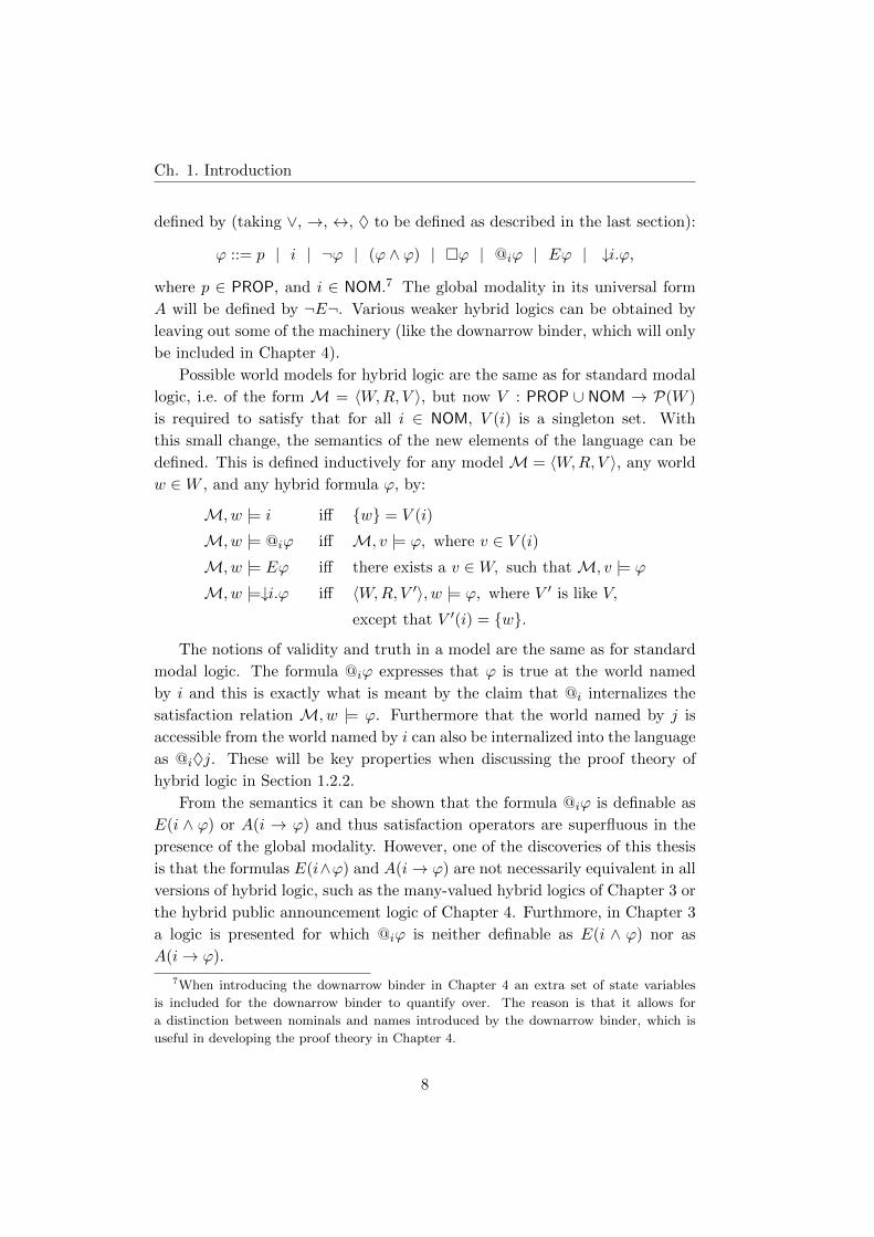
ϕ ::= p | i | ¬ϕ | (ϕ ∧ ϕ) | �ϕ | @iϕ | Eϕ | ↓i.ϕ,

where p ∈ PROP, and i ∈ NOM.7 The global modality in its universal form

A will be defined by ¬E¬. Various weaker hybrid logics can be obtained by

leaving out some of the machinery (like the downarrow binder, which will only

be included in Chapter 4).

Possible world models for hybrid logic are the same as for standard modal

logic, i.e. of the form M = 〈W,R, V 〉, but now V : PROP ∪ NOM → P(W )

is required to satisfy that for all i ∈ NOM, V (i) is a singleton set. With

this small change, the semantics of the new elements of the language can be

defined. This is defined inductively for any model M = 〈W,R, V 〉, any world

w ∈W , and any hybrid formula ϕ, by:

M, w |= i iff {w} = V (i)

M, w |= @iϕ iff M, v |= ϕ, where v ∈ V (i)

M, w |= Eϕ iff there exists a v ∈W, such that M, v |= ϕ

M, w |=↓i.ϕ iff 〈W,R, V ′〉, w |= ϕ, where V ′ is like V,

except that V ′(i) = {w}.

The notions of validity and truth in a model are the same as for standard

modal logic. The formula @iϕ expresses that ϕ is true at the world named

by i and this is exactly what is meant by the claim that @i internalizes the

satisfaction relation M, w |= ϕ. Furthermore that the world named by j is

accessible from the world named by i can also be internalized into the language

as @i♦j. These will be key properties when discussing the proof theory of

hybrid logic in Section 1.2.2.

From the semantics it can be shown that the formula @iϕ is definable as

E(i ∧ ϕ) or A(i → ϕ) and thus satisfaction operators are superfluous in the

presence of the global modality. However, one of the discoveries of this thesis

is that the formulas E(i∧ϕ) and A(i→ ϕ) are not necessarily equivalent in all

versions of hybrid logic, such as the many-valued hybrid logics of Chapter 3 or

the hybrid public announcement logic of Chapter 4. Furthmore, in Chapter 3

a logic is presented for which @iϕ is neither definable as E(i ∧ ϕ) nor as

A(i→ ϕ).

7When introducing the downarrow binder in Chapter 4 an extra set of state variables

is included for the downarrow binder to quantify over. The reason is that it allows for

a distinction between nominals and names introduced by the downarrow binder, which is

useful in developing the proof theory in Chapter 4.

8

1.1 The logic toolbox I: Modal logic and some of its friends

The extra added machinery of hybrid logic makes properties of models

and frames expressible that were not expressible in standard modal logic. It is

worth noticing that hybrid logic increases the expressive powers of modal logic,

sometimes even without an extra cost of increased complexity, see [7]. There

is much more to say about the expressive power of hybrid logic, but nothing

more will be said here. The chapters of this thesis dealing with hybrid logic

contain brief discussions of the expressivity of the presented hybrid logics. For

more on the expressivity of hybrid logic in general see [8, 146].

Another great advantage of hybrid logic is its nice and simple proof theory.

This has driven much recent research in hybrid logic, see [42]. The proof theory

of hybrid logic plays an important role in this thesis as chapters 2, 4, and 5

provide new proof theory for various hybrid logics. The proof theory of hybrid

logic will be properly introduced in Section 1.2.2.

Hybrid logic will appear in chapters 2, 3, 4, and 5 in slightly different

versions than the one presented here. First of all, due to the combination with

the public announcement operator8 in chapters 4 and 5 nominals will not be

required to be true in exactly one world, but in at most one world. The reason

for this modification to standard hybrid logic semantics is further described

in Chapter 4. Chapters 2 and 3 also contain a modification to the standard

hybrid logic semantics because the logics of these chapters are many-valued

logics. In a many-valued setting a statement like “the nominal i is true in

exactly one world” becomes ambiguous and the entire purpose of Chapter 3

is to investigate different possible semantics for nominals in a many-valued

setting.

The study of hybrid logic and modal logic has identified several interesting

fragments of first-order logic that turn up in other connections. Description

logic, which is a family of logics designed for knowledge representations, cor-

responds to many of the same fragments of first-order logic as hybrid logic

and modal logic. Moreover, description logic is interesting in its own right

in relation to modeling knowledge and information, and will briefly be used

in Chapter 7. Therefore a short elaboration of description logic will now be

given.

8The public announcement operator comes from dynamic epistemic logic and will be

discussed in more details in Section 1.1.5.

9

Ch. 1. Introduction

1.1.3 Description logic

Description logic is the result of a long development in formal knowledge rep-

resentation that has turned out to be a reinvention of not just modal logic,

but hybrid logic, [12]. However, there is much more to description logic than

just being a notational variant of some hybrid or modal logics. The entire

intuitions behind the formulas are different and the way the logic is used for

knowledge representation gives rise to a new large family of reasoning tasks

other than the standard search for validities. This section will elaborate on

the intuitions behind description logic and present a little of the formal syn-

tax and semantics of the logic. How description logic is used in knowledge

representation will be the topic of Section 1.3.2.1.

Two kinds of knowledge about the world (or a specific domain) can be

distinguished, namely terminological knowledge and world assertions. Termi-

nological knowledge is knowledge about the structure of the concepts used to

describe the world, whereas world assertions are descriptions of which indi-

viduals exist and which concepts they satisfy. Thus, the basics are no longer

propositions, but concepts or concept descriptions.

Formally, concept descriptions are built up from a set of atomic concepts

(usually denoted by A or B) and a set of atomic roles (usually denoted by R)

using concepts or role constructors. Given these two sets, concept descriptions

are built up by the following syntax:

C ::= A | > | ⊥ | ¬C | (C u C) | (C t C) | ∃R.C | ∀R.C,

where A is an atomic concept and R is an atomic role. This language is usually

denoted ALC. Several sublanguages and extensions of ALC exist as well.

An example of a concept description is Woman u ∀hasChild(RedHair tBlueEyes) describing all women all of whose children either have red hair or

blue eyes. To ensure this reading a formal semantics is given to concept de-

scriptions based on the standard set-theoretic semantics of first-order logic,

since concepts can be viewed as unary predicates and roles as binary rela-

tions. An interpretation I consists of a non-empty domain ∆I and a function

that to each atomic concept A assigns a set AI ⊆ ∆I and to each atomic role

R assigns a binary relation RI ⊆ ∆I × ∆I . The interpretation function is

then extended to all concept descriptions, yielding subsets of the domain ∆I ,

10

1.1 The logic toolbox I: Modal logic and some of its friends

in the following inductive way:

>I = ∆I

⊥I = ∅(¬C)I = ∆I \ CI

(C uD)I = CI ∩DI

(C tD)I = CI ∪DI

(∃R.C)I = {a ∈ ∆I | ∃b : (a, b) ∈ RI and b ∈ CI}(∀R.C)I = {a ∈ ∆I | ∀b : if (a, b) ∈ RI then b ∈ CI}

From the formal semantics it is easy to see that the language ALC is just a

notational variant of standard modal logic, since C uD corresponds to C ∧D,

CtD corresponds to C∨D, ∃R.C corresponds to ♦RC9, and so on. However,

further extensions of ALC add machinery that makes it into variants of hybrid

logic, modal logic with counting quantifiers, or other extended modal logics.

For more on the relationship between description logic and modal logic, see

[13, 135].

With a formal syntax and semantics for concept descriptions, description

logic can now be used to represent knowledge of the world. To do this, another

layer is added to description logic, keeping the distinction between terminolog-

ical knowledge and world assertions in mind, namely TBoxes (terminological

boxes) and ABoxes (assertion boxes). A TBox contains terminological knowl-

edge about the world in the form of inclusion axioms C v D or equality axioms

C ≡ D between concept descriptions C and D, for instance Woman v Human

or Human ≡ Woman t Man, expressing that all women are humans or that

humans are defined as either being a woman or a man. An interpretation I is

said to satisfy a TBox T if, for all axioms C v D in T , CI ⊆ DI , and for all

axioms C ≡ D in T , CI = DI .

An ABox contains concrete assertions about the world in the form of con-

cept assertions C(a) or role assertions R(a, b). Here a and b are names of indi-

viduals coming from a fixed set of names introduced for expressing world asser-

tions. Thus, an ABox can contain concrete knowledge such as Woman(Maria)

expressing that Maria is a woman, or hasChild(Maria,Peter) expressing that

Peter is a child of Maria. The notion of an interpretation I is then extended

such that it assigns an object aI ∈ ∆I for each name a. An interpretation

9A modal logic can contain several modalities in which case the modalities are indexed

as in ♦R. Then, in the semantics an accessibility relation R is specified for each modality

♦R and used interpreted formulas ♦Rϕ.

11

Ch. 1. Introduction

I is then said to satisfy an ABox A if aI ∈ CI , for all assertions C(a) in Aand (aI , bI) ∈ RI , for all assertions R(a, b) in A. Note that assertions from

ABoxes can be internalized into the syntax of concept descriptions, exactly as

hybrid logic internalizes the semantics of modal logic.10 Thus, the resulting

description logic becomes a notational variant of hybrid logic.

With ABoxes and TBoxes, knowledge about the world can be represented

in a uniform and concise way. However, description logic offers more than just

a smart language for representing knowledge. Due to the formal semantics,

TBoxes and ABoxes can contain a great deal of implicit knowledge which can

be uncovered by description logic reasoning. Given a TBox T and a concept

description C one can ask whether C is satisfiable with respect to T , that is,

whether there is an interpretation I that satisfies T and such that CI is non-

empty. Furthermore, one can ask whether C is subsumed by D with respect to

T , that is, whether for all interpretations I that satisfy T , CI ⊆ DI . Similarly,

one can ask whether two concept descriptions are equivalent or whether they

are disjoint. However, in several description logics these tasks can be reduced

to one another. More advanced reasoning tasks can be obtained by combining

other reasoning tasks. For instance one can ask for all the implicit subsumption

relationships between concepts that follow from a TBox, and thereby obtain

a classification of the TBox – a task useful in many applications (such as in

medical ontologies) and further discussed in Section 1.3.2.1. Given an ABox

and a TBox one can ask whether the ABox contains a possible description

of the world, in other words whether it is consistent relative to the given

TBox. This question amounts to asking whether there is an interpretation

that satisfies both the TBox and the ABox simultaneously. Furthermore, one

can ask whether an individual a always satisfies a concept C relative to a

TBox and an ABox, or whether the role R is satisfied for individuals a and b,

or what the most specific concept (relative to the ordering v) that describes

a given individual a is.

Even though many of the reasoning tasks for description logic can be re-

duced to each other, very efficient reasoning procedures have been developed

for the individual tasks in minimal languages. In general, the research and

development of description logic have been highly motivated by the wish for

efficient implementations. The development of these efficient implementations

10Allow for names of individuals to appear as atomic concept and let the interpretation of

the name a, when appearing as a concept, be the set {aI}. Then an interpretation satisfies

C(a) if and only if the concept a u C is non-empty and it satisfies R(a, b) if and only if the

concept a u ∃R.b is non-empty.

12

1.1 The logic toolbox I: Modal logic and some of its friends

has made description logic very useful for knowledge representation. For more

on description logic and its applications see [12].

In Chapter 7, mainly first-order logic is used to discuss how knowledge

representation of regulatory relations can be done. However, the chapter also

discusses how description logic can be used, as well as what further research on

description logic could be valuable for this kind of knowledge representation

– an issue returned to in Section 1.3.2.1.

Description logics are logics tailored to representing, structuring, and rea-

soning about domain knowledge, which makes them very useful for applica-

tions that aim at developing automatic tools for handling large amounts of

information. The value of description logics for such applications will be ex-

plained further in Section 1.3.2.1. When it comes to reasoning about the

knowledge possessed by individuals and knowledge about other individuals’

knowledge, a logic that makes explicit references to the individuals and their

subjective knowledge is needed. Epistemic logic is a logic that does exactly

this.

1.1.4 Epistemic logic

Epistemic logic is essentially merely a subfield of modal logic, dealing with

modalities involving knowledge and beliefs.11 However, epistemic logic is in-

teresting in its own right and has been widely studied. This section discusses

exactly how epistemic logic fits in with standard modal logic and its possible

world semantics, and how it extends standard modal logic.

A first addition made by epistemic logic to standard modal logic is to

include several modalities, one for each agent coming from a fixed, finite set

of agents (which will be denoted A in the following). Therefore, models of

epistemic logic do not contain a single accessibility relation, but one for each

agent a ∈ A. The standard modalities of epistemic logic are “agent a knows

that” and “agent a believes that”, usually represented as Ka and Ba (for all

a ∈ A). However, introducing notions of group knowledge and beliefs, other

important modalities become “it is common knowledge among the agents in

the group G that” and “it is distributed knowledge among the agents in the

group G that” (represented as CG and DG), and similar for beliefs. Moreover,

11Sometimes the term “epistemic logic” is used only for logics that deal with modalities

involving knowledge and the term “doxastic logic” is then used to refer to logics dealing with

belief modalities. However, in the rest of this thesis the term “epistemic logic” will be used

for all logics dealing with knowledge or beliefs modalities.

13

Ch. 1. Introduction

some uncommon modalities will also be discussed in Chapter 6, namely “agent

a is ignorant about” and “agent a doubts whether”.

Epistemic logic, in some form, was already being investigated in ancient

and medieval logic [34, 73], but modern epistemic logic was first thoroughly

initiated by Hintikka’s book “Knowledge and Belief – An Introduction to the

Logic of the Two Notions” [96]. Even though it was within philosophy that

epistemic logic started, it has been commonly used within computer science

since the 1980s [57, 119] and within game theory since the 1990s [11, 19], and

the many applications of epistemic logic have helped shape the field ever since.

From the time of Hintikka’s work, possible world semantics has been widely

accepted as the standard semantics for epistemic logic, and has also motivated

many of the applications.12 The possible world semantics reflects the view that

something is known to an agent if it is true in all the alternative situations

(possible worlds) that the agent can conceive of as possible. Thus, gaining

more knowledge corresponds to eliminating more worlds. This view on knowl-

edge, or information, is referred to as “information as range” by Johan van

Benthem [1, 155]. How logic in general deals with information is discussed in

more details in Section 1.3.2.

The modalities Ka, Ba, CG, and DG are all interpreted in the possible

world semantics as the � modality of standard modal logic, which for the case

of Ka exactly gives rise the view of information as range. Usually, for the

modality Ka, further requirements are put on the corresponding accessibility

relation Ra in the possible world semantics. The most common requirement

is to assume that Ra is an equivalence relation13 for all agents a ∈ A. The

set of formulas that are valid on the class of frames where all accessibility

relations are equivalence relations is called the modal logic S5.14 There has

been considerable philosophical debate about whether S5 is too strong a logic

for knowledge, since it makes the agents negatively introspective, that is it

validates the axiom ¬Kaϕ→ Ka¬Kaϕ expressing that whatever agent a does

not know, a knows that he does not know. Weaker logics like S4(where Ra is

only assumed to be reflexive and transitive) have been suggested, but in the

many applications in computer science [57] and game theory [11, 160] it has

12Other semantics than the possible world semantics are possible for epistemic logic, but

in this thesis only possible world semantics is considered for epistemic logic as it appears in

chapters 4, 5, and 6.13That Ra is an equivalence relation means that Ra is reflexive (∀x(Ra(x, x))), symmetric

(∀x∀y(Ra(x, y)→ Ra(y, x))) , and transitive (∀x∀y∀z(Ra(x, y) ∧Ra(y, z)→ Ra(x, z))).14Given a class of frames, the set of formulas valid on that class is referred to as a logic.

14

1.1 The logic toolbox I: Modal logic and some of its friends

turned out that the logic S5 best captures the required notion of knowledge.15

In Chapter 6, S5 is assumed as the logic of knowledge, but in chapters 4 and

5 no assumption is put on the accessibility relation.16

When the belief modality Ba is interpreted in possible world semantics

it is also as the � modality with further requirement on the corresponding

accessibility relation. The accessibility relation is usually required to be serial,

transitive, and Euclidean17 giving rise to the logic KD45.18 Chapter 6 is the

only chapter dealing explicitly with beliefs, however, essential to that chapter

is how beliefs change under public announcements and the logic KD45 does not

work well with public announcements, a matter returned to in Section 1.2.3.

Instead, in Chapter 6, the framework of plausibility models will be used.

A plausibility model is a possible world modelM = 〈W, (≤a)a∈A, V 〉, where

the accessibility relations ≤a are assumed to be locally connected, converse

well-founded preorders. A relation is locally connected if; whenever x and y

are related (either x ≤a y or y ≤a x holds) and y and z are related, then x

and z are also related; a relation on W is converse well-founded if; every non-

empty subset of W has a maximal element; and a relation is a preorder if it is

reflexive and transitive. Furthermore, equivalence relations ∼a on W can be

defined by requiring that w ∼a v if, and only if either w ≤a v or v ≤a w. The

resulting equivalence class |w|a = {v ∈ W | v ∼a w} is called the information

cell of agent a at w. The semantics of the belief modality Ba can then be

15Assuming that S5 is the right logic for knowledge corresponds to assuming that the

formulas Kaϕ→ ϕ, Kaϕ→ KaKaϕ, and ¬Kaϕ→ Ka¬Kaϕ are valid. Thus S5 is the logic

in which it is assumed that: whatever is known to an agent is true, whenever an agent knows

something the agent knows this fact, and whenever an agent does not knows something the

agent knows this fact. Accepting these properties is one way of arguing for S5. Another way

is by assuming that the relation Ra is an epistemic indistinguishability relation for agent a

in which it is natural to assume that: a cannot distinguish the actual from itself, if a cannot

distinguish the world v from w, the a distinguish w from v either, and if a cannot distinguish

v from w and u from v, then a cannot distinguish u from w either.16Due to automatic completeness with respect to pure formulas in hybrid logic, which will

be discussed in Section 1.2.2, it is easy to extend the results of Chapter 4 to the case of S4

or S5.17A relation R is serial if ∀x∃y(R(x, y)) and Euclidean if ∀x∀y∀z(R(x, y) ∧ R(x, z) →

R(y, z)).18When moving from knowledge to belief the requirement that knowledge implies truth

(Kaϕ→ ϕ should be abandoned since a belief in ϕ does not ensures that ϕ is actually true

– beliefs can be wrong. However beliefs should be consistent in the sense that an agent

should never believe ϕ and ¬ϕ at the same time. The change corresponds to replacing the

requirement of reflexivity with the requirement of seriality on the accessibility relation, which

again corresponds to moving from the logic S5 to KD45.

15

Ch. 1. Introduction

defined by:

M, w |= Baϕ iff for all v ∈ max≤a(|w|a),M, v |= ϕ.

The intuition behind the fact w ≤a v is that agent a thinks that the world v is

at least as plausible as world w, but a cannot tell which of the two is the case.

Furthermore, an agent believes something to be the case if it is true in the

worlds that the agent considers most plausible. For more on the plausibility

framework see Chapter 6.

The semantics of the common knowledge modality CG and the distributed

knowledge DG modality is a little more involved. For relations (Ra)a∈A new

relations⋃a∈ARa and

⋂a∈ARa can be defined as the set theoretic union, or the

set theoretic intersection, respectively, of the relations (Ra)a∈A. Furthermore,

for a relation R, R∗ will denote the reflexive transitive closure of R, that is

the smallest relation that extends R and is reflexive and transitive. With

these definitions fixed, given a possible world model M = 〈W, (Ra)a∈A, V 〉and a G ⊆ A, the semantics of the common knowledge modality CG and the

distributed knowledge DG modality can be defined by:

M, w |= CGϕ iff for all v ∈W, if (w, v)∈(⋃

a∈GRa)∗

then M, v |= ϕ

M, w |= DGϕ iff for all v ∈W, if (w, v)∈(⋂

a∈GRa)

then M, v |= ϕ.

That something is common knowledge means that everybody knows it and

that everybody knows that everybody knows it... and so on. Thus common

knowledge can be viewed as an infinite conjunction. This intuition is captured

by the given formal semantics. That something is distributed knowledge has

the intuition that, if the agents pull all their knowledge together they will

know it. Hence, for distributive knowledge, only the worlds that all the agents

consider possible need to be consulted, which leads to the given formal seman-

tics.

For many of the applications of epistemic logic it is not just knowledge

and belief that are important, but also how knowledge and beliefs of agents

evolve over time or during a process. In the next section one approach to

the dynamics of knowledge and beliefs is further discussed, namely dynamic

epistemic logic.

1.1.5 Dynamic epistemic logic

Dynamic aspects of knowledge and beliefs have been studied in logic for some

time, for instance in belief revision [5, 85] or interpreted systems [78, 57, 125].

16

1.1 The logic toolbox I: Modal logic and some of its friends

However, recently dynamic epistemic logic has emerged as an alternative ap-

proach. In interpreted systems the dynamics of knowledge and beliefs are

hardwired into the system by specifying all the possible runs of the systems

as well as how the states of the system can change due to certain actions.

Therefore, the entire system and all its future developments have to be speci-

fied from the beginning of a modeling process. Dynamic epistemic logic takes

another approach, where only the starting state of the system needs to be

specified and the future evolution of the system is completely given by the

actions performed. So, instead of modeling a system by specifying all the pos-

sible runs, one specifies the possible actions instead. This gives a local view of

the dynamics of knowledge and beliefs that has proved quite useful in several

applications. The applications of dynamic epistemic logic include: verifica-

tion of security protocols for communications [164, 50, 51, 95, 4], automated

epistemic planning [35, 108], reasoning about quantum computation and in-

formation [16, 18], elucidating the foundation of game theory [160, 156, 47],

modeling dialogues and communication in linguistics and philosophy of lan-

guage [113] as well as speech acts [105, 106]. In this section the syntax and

semantics of dynamic epistemic logic are formally introduced and several issues

relevant for this thesis are elaborated.

Dynamic epistemic logic is a term used to cover extensions of epistemic

logic that add dynamic modalities (as in dynamic logic [86, 165]), representing

actions with epistemic effects, to model the dynamics of knowledge and beliefs.

However, instead of interpreting these dynamic modalities as quantifying over

possible worlds within a given model, in dynamic epistemic logic the dynamic

modalities quantify over transformations of possible world models. In most

versions of dynamic epistemic logic, actions having only epistemic effects are

considered. For dynamic epistemic logics that can change the fact of the world

as well see [162, 157, 105]. Actions only having epistemic effect will also be

referred to as epistemic actions.

The simplest version of dynamic epistemic logic, though still giving rise

to numerous applications, is public announcement logic, which goes back to a

paper by Plaza in 1989 [128], but was also independently developed in the late

1990s by Gerbrandy and Groeneveld [70, 69]. Public announcement logic adds

one type of dynamic modality to standard epistemic logic, namely modalities of

(truthful) public announcements. To the syntax of epistemic logic a modality

[ϕ] is added for every formula in the language, giving rise to complex formulas

of the form [ϕ]ψ having the intuitive reading “after public announcement of

ϕ, ψ is the case”. When a truthful announcement of ϕ takes place it means

17

Ch. 1. Introduction

that no agent any longer considers worlds possible where ϕ was not true.19 In

the formal semantics this simply corresponds to moving the evaluation of a

formula to the submodel consisting only of worlds that make ϕ true. Formally,

for any model M = 〈W, (Ra)a∈A, V 〉, any w ∈ W , and any formulas of the

language ϕ and ψ, the following clause is added to the inductive definition of

the relation |=:

M, w |= [ϕ]ψ iff M, w |= ϕ implies that M|ϕ, w |= ψ,

where M|ϕ = 〈W |ϕ, (Ra|ϕ)a∈A, V |ϕ〉 is the submodel defined by

W |ϕ = {w ∈W | M, w |= ϕ}Ra|ϕ = Ra ∩ (W |ϕ ×W |ϕ) , for all a ∈ AV |ϕ(p) = V (p) ∩W |ϕ , for all p ∈ PROP.

Normally public announcement logic is viewed as an extension of epistemic

logic and therefore the underlying accessibility relations are assumed to be

equivalence relations. However, a more general approach will be taken in this

thesis, and unless particularly mentioned, no particular assumption on the

accessibility relation will be made. Nevertheless, all results, except the ones in

Chapter 5, are easily extendable to the case where the accessibility relations

are equivalence relations.

As already indicated, the modality [ϕ] models the truthful announcement

of ϕ, which is the reason for the antecedent requirement “M, w |= ϕ” in the

definition of the semantics of [ϕ]ψ. This means that a public announcement

[ϕ] is always treated as incoming true information for all agents of the model

which result in them all coming to know that ϕ was the case. Furthermore,

this is all common knowledge among the agents in the model, which is the

reason for the term “public”.

The presented syntax and semantics for public announcements also fit

nicely with the plausibility framework introduced in the last section. The just

presented semantic for the public announcement operator is used on plausi-

bility models as well. However, in Chapter 6 where the logic of plausibility

models is used together with public announcements, other announcements that

19A public announcement of ϕ does not guarantee that ϕ becomes true. Take for instance

the Moore sentence “p is true but a does not know it”. After a public announcement of

this formula, a does know p and the Moore sentence therefore becomes false. However,

the Moore sentence was true at the moment of the announcement. This issue leads to a

distinction between successful and unsuccessful formulas, see Section 4.7 in [163].

18

1.1 The logic toolbox I: Modal logic and some of its friends

changes the plausibility relation instead of deleting worlds are also introduced.

In chapters 4 and 5 public announcement logic will be combined with hybrid

logic as introduced in Section 1.1.2.

Expressiveness and succinctness are important issues for public announce-

ment logic. Due to the following validities in public announcement logic

[ϕ] p ↔ (ϕ→ p) (1.1)

[ϕ]¬ψ ↔ (ϕ→ ¬[ϕ]ψ) (1.2)

[ϕ] (ψ ∧ χ) ↔ ([ϕ]ψ ∧ [ϕ]χ) (1.3)

[ϕ]Kaψ ↔ (ϕ→ Ka[ϕ]ψ) (1.4)

[ϕ] [ψ]χ ↔ [ϕ ∧ [ϕ]ψ]χ, (1.5)

every formula of public announcement logic can be transformed into an equiv-

alent20 formula of standard epistemic logic without public announcements.

Thus, the addition of public announcement modalities [ϕ] to epistemic logic

does not increase the expressive power of the logic in the sense that nothing

new can be expressed, [163]. This is also the case if the distributed knowledge

modality or any of the hybrid machinery of Section 1.1.2 are added to stan-

dard epistemic logic, which is shown in Chapter 4. However, adding public

announcement modalities to epistemic logic with common knowledge does in-

crease the expressive power of the logic – one reason for this is briefly discussed

in Section 4.4.5 of Chapter 4. Although public announcements do not add to

the expressive power of epistemic logic (with the exception of epistemic logic

with common knowledge) they do add to the succinctness of epistemic logic.

With public announcements, propositions can be expressed much shorter than

in standard epistemic logic [115] (at least for the case where no requirements

are put on the accessibility relations). The validities (1.1)− (1.5) are usually

referred to as reduction axioms because they play an important role in the

proof theory of public announcement logic. The proof theory of public an-

nouncement logic will be presented in Section 1.2.3 and will be the topic of

chapters 4 and 5.

Public announcements are just one simple type of epistemic action corre-

sponding to the simple transformation on possible world models of moving

to submodels. However, the real power of dynamic epistemic logic is ob-

tained when a wider range of more complex epistemic actions are dealt with

20Two formulas ϕ and ψ are said to be equivalent if for all models M = 〈W, (Ra)a∈A, V 〉and all w ∈W , M, w |= ϕ if, and only if M, w |= ψ.

19

Ch. 1. Introduction

in a uniform manner by transformations on possible world models. The ap-

proach that has become the dominant one, initially developed by Baltag, Moss,

and Solecki [15], interprets dynamic epistemic modalities as “action models”,

which, through a product operation, transform possible world models and

thereby bring dynamics into epistemic logic.

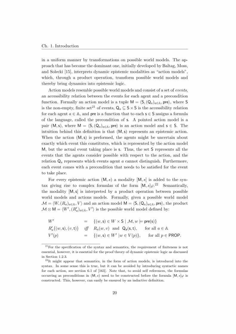
Action models resemble possible world models and consist of a set of events,

an accessibility relation between the events for each agent and a precondition

function. Formally an action model is a tuple M = 〈S, (Qa)a∈A, pre〉, where S

is the non-empty, finite set21 of events, Qa ⊆ S× S is the accessibility relation

for each agent a ∈ A, and pre is a function that to each s ∈ S assigns a formula

of the language, called the precondition of s. A pointed action model is a

pair (M, s), where M = 〈S, (Qa)a∈A, pre〉 is an action model and s ∈ S. The

intuition behind this definition is that (M, s) represents an epistemic action.

When the action (M, s) is preformed, the agents might be uncertain about

exactly which event this constitutes, which is represented by the action model

M, but the actual event taking place is s. Thus, the set S represents all the

events that the agents consider possible with respect to the action, and the

relation Qa represents which events agent a cannot distinguish. Furthermore,

each event comes with a precondition that needs to be satisfied for the event

to take place.

For every epistemic action (M, s) a modality [M, s] is added to the syn-

tax giving rise to complex formulas of the form [M, s]ϕ.22 Semantically,

the modality [M, s] is interpreted by a product operation between possible

world models and actions models. Formally, given a possible world model

M = 〈W, (Ra)a∈A, V 〉 and an action model M = 〈S, (Qa)a∈A, pre〉, the product

M⊗M = 〈W ′, (R′a)a∈A, V ′〉 is the possible world model defined by:

W ′ = {(w, s) ∈W × S | M, w |= pre(s)}R′a((w, s), (v, t)

)iff Ra(w, v) and Qa(s, t), for all a ∈ A

V ′(p) = {(w, s) ∈W ′ |w ∈ V (p)}, for all p ∈ PROP.

21For the specification of the syntax and semantics, the requirement of finiteness is not

essential, however, it is essential for the proof theory of dynamic epistemic logic as discussed

in Section 1.2.3.22It might appear that semantics, in the form of action models, is introduced into the

syntax. In some sense this is true, but it can be avoided by introducing syntactic names

for each action, see section 6.1 of [163]. Note that, to avoid self references, the formulas

occurring as preconditions in (M, s) need to be constructed before the formula [M, s]ϕ is

constructed. This, however, can easily be ensured by an inductive definition.

20

1.1 The logic toolbox I: Modal logic and some of its friends

The formal semantics of the action modality [M, s] can now be defined by:

M, w |= [M, s]ϕ iff M, w |= pre(s) implies that M⊗M, (w, s) |= ϕ.

The requirement ofM, w |= pre(s) for (w, s) to be included in W ′, reflects the

idea that the precondition pre(s) needs to be satisfied in a world before the

event s can take place in that world. The definition of R′a reflects the intuition

that an agent can distinguish between two resulting worlds (w, s) and (w′, s′),

either if the agent can distinguish between the original worlds w and w′ or

if the agent can distinguish the events s and s′ as they occur. Finally, the

definition of V ′ reflects the fact that epistemic actions cannot change the fact

of the world, represented by the value of the propositional variables in PROP.

It is worth noticing that dynamic epistemic logic with action models is a

genuine generalization of public announcement logic, since public announce-

ments can be described by action models. Given a formula ϕ, a public an-

nouncement of ϕ corresponds to the action model 〈{s0}, {(s0, s0)}, {(s0, ϕ)}〉.It is easy to see that this action model results in the same model transforma-

tions as the public announcement operator [ϕ].

Surprisingly, as in the case of public announcements, adding action modal-

ities of the form [M, s] to epistemic logic does not increase the expressive power

of the language. This is again due to the existence of valid reduction axioms:

[M, s] p ↔(pre(s)→ p

)(1.6)

[M, s]¬ϕ ↔(pre(s)→ ¬[M, s]ϕ

)(1.7)

[M, s] (ϕ ∧ ψ) ↔([M, s]ϕ ∧ [M, s]ψ

)(1.8)

[M, s]Kaϕ ↔(pre(s)→

∧Ra(s,t)

Ka[M, t]ϕ)

(1.9)

[M, s] [M′, s′]ϕ ↔ [(M; M′), (s, s′)]ϕ, (1.10)

where, in the last formula, the “;” operation is a semantic operation on

action models: Given two action models, M = 〈S, (Qa)a∈A, pre〉 and M′ =

〈S′, (Q′a)a∈A, pre′〉, the composition (M; M′) = 〈S′′, (Q′′a)a∈A, pre′′〉 is defined by:

S′′ = S× S′

Q′′a((s, s′), (t, t′)

)iff Qa(s, t) and Q′a(s′, t′)

pre′′((s, s′)) = 〈M, s〉pre′(s′).

As for public announcement logic, adding action modalities to epistemic logic

with common knowledge increases the expressive power. However, whether

21

Ch. 1. Introduction

adding action modalities to a hybrid version of epistemic logic increases the

expressive power, is still an open problem. Normally, nominals in hybrid logic

are true in exactly one (or at most one) world, but a world w in a possible

world model can turn into several worlds (w, s) when a product is taken with

an action model. Thus, there seems to be no single obvious way of defining

the semantics of nominals in the presence of action models.

Action models will only appear in Chapter 5 where the reduction axioms

(1.6) − (1.10) are used as rules for a tableau system for epistemic logic with

epistemic actions. As mentioned above, the proof theory of dynamic epistemic

logic is discussed in Section 1.2.3, but before turning to proof theory, one final

extension of standard modal logic is discussed.

1.1.6 Many-valued logics

Even though modal logic, and the extensions presented here, are often catego-

rized as non-classical logic, they are still classical in the sense that propositions

are assumed to be either true or false, and not allowed to be neither or both.

This assumption of only two possible truth values is a simplification in several

scenarios. Many-valued logic steers clear of this assumption by allowing all

sorts of sets to play the role of truth values. However, arbitrary sets are not

allowed as truth values, the sets need to have particular structures for the

logics to be interesting. Even with this limitation there is still a plenitude of

many-valued logics.

For each class of particular structures, a family of many-valued logics arises.

In this thesis only one such family will be considered, namely the family arising

from requiring that the sets of truth values are finite Heyting algebras. A finite

Heyting algebra is a finite lattice where every element has a relative pseudo-

complement. A lattice is a partially ordered set23 L = 〈L,≤〉 where every two

elements x, y ∈ L always have a least upper bound and a greatest lower bound.

For x, y ∈ L the least upper bound is also called a join, denoted by xty and the

greatest lower bound is also called a meet, denoted by xuy.24 Since only finite

Heyting algebras, and thus only finite lattices, are considered, all the lattices

will be bounded and complete. This means that all the lattices L = 〈L,≤,t,u〉will contain a smallest element, denoted ⊥ and largest element, denoted >, and

that for all subsets A ⊆ L the join⊔A (the least upper bound of the set A)

and the meetdA (the greatest lower bound of the set A) can be formed. That

23That is, the relation ≤ is reflexive, anti-symmetric, and transitive.24The u and t is not to be confused with the description logic concept constructors.

22

1.1 The logic toolbox I: Modal logic and some of its friends

all elements of a lattice L = 〈L,≤,t,u〉 have a relative pseudo-complement

means that, for all a and b in L, there is a greatest element x ∈ L satisfying

a u x ≤ b. The element x is called the relative pseudo-complement of a with

respect to b and will be denoted by a ⇒ b. For more on lattices, orders, and

Heyting algebras see [48, 33].

The structure of the Heyting algebra allows for natural interpretation of

the standard logical connectives; ∧ is interpreted as u, ∨ is interpreted as t,

→ is interpreted as ⇒, > is interpreted as the largest element of the Heyting

algebra (also denoted >), and ⊥ is interpreted as the smallest element of the

Heyting algebra (also denoted ⊥).

A possible intuition behind adopting finite Heyting algebras as sets of truth

values is given by Fitting in [60, 61, 63], where each truth value is viewed as

a subset of a set of experts and the Heyting algebra structure comes from

assuming a possible relation of dominance between the agents. Viewing truth

values as sets of experts or agents will give way to an application described in

Section 1.3.3.

Many-valued logics, where the sets of truth values are finite Heyting al-

gebras, have been combined with modal logic by Fitting in [59, 60, 61]. In

his many-valued modal logic, propositions are assigned truth values from a

fixed Heyting algebra at each world, and furthermore, the accessibility be-

tween worlds is also assigned values from the Heyting algebra.25 Chapters 2

and 3 concern an extension of this many-valued modal logic to a hybrid logic

version.

In Chapter 2 it is shown that the many-valued modal logic of Fitting can

be extended to a hybrid version, which shows the great universality of hybrid

logic. However, as already mentioned, the semantics of the hybrid machinery

in a many-valued setting can be defined in several ways, and even though the

way it is defined in Chapter 2 results in a many-valued hybrid logic inheriting

many of the properties of standard hybrid logic, there are other natural ways

of defining the semantics of the hybrid machinery in a many-valued setting,

and this is the topic of Chapter 3.

One of the properties that the many-valued hybrid logic of Chapter 2

inherits from standard hybrid logic is a nice proof theory. The next section

discusses proof theory in more detail.

25Another reason for assuming the set of truth values to be a finite Heyting algebra

is that the notion of relative pseudo-complement allows for a natural way of interpreting

the modalities when the accessibility relation is also many-valued. See Chapter 2 for the

definition of the semantics of the modalities.

23

Ch. 1. Introduction

1.2 The logic toolbox II: Proof theory

Proofs have played a role in mathematics since at least ancient times and the

rigorous presentation of geometry in Euclid’s Elements has been a paradig-

matic example of mathematical proofs ever since. Proof theory does not as

such study mathematicians’ proofs, but rather formal versions of proofs. As

a subfield of logic, proof theory grew out of the problems of finding a firm

foundation for mathematics, most famously explored by Hilbert and subse-

quently referred to as “Hilbert’s program” [174]. Hilbert realized that a firm

foundation for mathematics must rely on logic, something Frege and Russell

had already worked on, and in the process he developed an axiomatic proof

theory that dominated around 1920 [169]. This style of proof theory is re-

ferred to as “Hilbert-style proof systems” or “Hilbert-style axiom systems”.

Since then several other proof systems have been developed such as natural

deduction, sequent calculus (both developed by Gentzen), tableau system (de-

veloped by Beth), and resolution (developed by Robinson). In this thesis only

Hilbert-style proof systems (Chapter 4) and tableau systems26 (chapters 2 and

5) are considered. Therefore, the next section gives a short introduction to

Hilbert-style proof systems and tableau systems for modal logic, other proof

systems for modal logic can be found in [62]. Furthermore, since the logics of

chapters 4, 2, and 5 are all hybrid logics, the proof theory of hybrid logic will

be discussed in Section 1.2.2, and the proof theory of dynamic epistemic logic

will be discussed in Section 1.2.3 since chapters 4 and 5 also contribute to the

proof theory of dynamic epistemic logic.

1.2.1 The proof theory of modal logic

While the semantic (or model theoretic) tradition in logic approaches the

problem of the validity of arguments through a notion of truth, proof theory

approaches the problem through a notion of proofs – an argument is proof-

theoretical valid if the conclusion can be proved from the premises. However,

within proof theory much effort is put into showing that the proof-theoretical

notion of validity coincides with the semantic notion of validity. In the rest of

this thesis when referring to a notion of validity it will always be a semantic

notion of validity. When a formula is proof-theoretical valid it will usually

be referred to as provable instead. Thus, the semantic notion of validity will

26Sequent calculus and tableau systems are closely connected and for the basic logics they

give rise to equivalent proof systems.

24

1.2 The logic toolbox II: Proof theory

be taken as primary, and one of the main task of proof theory will be the

task of capturing the semantic notion of validity by a notion of proof.27 As

stated by Fitting in [62], a formal proof is a finitary certificate of the validity

of a formula (or an argument). A proof system is something that specifies

whether a given object counts as a formal proof of a formula or not. Thus, the

objective of proof theory is to develop proof systems that guarantee that every

valid formula has a formal proof and that no invalid formula has a formal proof.

Moreover, proof theory is a syntactic approach to the validity of arguments,

since proof systems specify rules and axioms that lead to formal proofs based

on the syntactic structure of formulas without taking the meaning/semantics

of the formulas into account.

When developing a proof system for a given logic, as already mentioned,

it is important that every valid formula has a formal proof and that no in-

valid formula has a formal proof. The property that every valid formula has

a formal proof is referred to as completeness of the proof system. The prop-

erty that no invalid formula has a formal proof is referred to as soundness

of the proof system. Besides completeness and soundness, another important

property of some proof systems is the question of whether they give rise to

a decision procedure for the logic. A decision procedure is an algorithm that

always terminates and for any formula of the logic tells whether it is valid or

not. If such a decision procedure exists, the logic is said to be decidable.

In Hilbert-style proof systems, a proof of a formula ϕ is a finite sequence

of formulas where each formula in the sequence is either an axiom (from a

fixed set of axioms) or follows by a rule (from a fixed set of rules) from for-

mulas earlier in the sequence, and where the last formula of the sequence is

ϕ. Hence, to specify a Hilbert-style proof system one needs to specify a set of

axioms (a particular set of formulas) and a set of rules (a rule takes a fixed

finite number of formulas of certain types and returns a single formula). A

typical way of giving a Hilbert-style proof system for standard modal logic is

shown in Figure 1.1.28

27This view puts proof theory secondary to semantics, which of course is debatable from

a philosophical point of view. The field of proof-theoretic semantics is an example of an

approach that takes the notion of proofs prior to a semantic notion of truth.28In several definitions of Hilbert-style proof systems for modal logic an additional rule is

included, which states that from a formula ϕ, any formula ϕ′ obtained from ϕ by uniformly

substituting modal formulas for propositional variables in ϕ may be inferred. However, such

a rule does not preserve validity for dynamic epistemic logic and has therefore been left out

in all Hilbert-style proof systems in this thesis. The way the axiom (Tau) is formulated

25

Ch. 1. Introduction

Axioms:

All substitution instances of propositional tautologies (Tau)

�(ϕ→ ψ)→ (�ϕ→ �ψ) (K)

Rules:

From ϕ and ϕ→ ψ infer ψ (Modus ponens)

From ϕ infer �ϕ (Necessitation)

Figure 1.1: A Hilbert style proof system for standard modal logic

A few comments are in order. By “substitution instances of propositional

tautologies” is meant that whenever ϕ is a tautology, then ϕ′, obtained by

uniformly substituting modal formulas for propositional variables in ϕ, is also

an axiom, for instance �p ∨ ¬�p is an axiom. The axiom (K) is actually an

axiom scheme (and so is (Tau)), that is, it represents infinitely many axioms,

one for every pair of modal formulas ϕ and ψ. In the following, axiom schemes

will also be referred to just as axioms, whenever there is no risk of confusion.

A similar issue is the case for the rules; a rule like (Necessitation) is intended

to be applicable to any pair of formulas ϕ and ϕ → ψ. Finally, in this proof

system ♦ is taken to be defined in the syntax as ¬�¬, otherwise an axiom of

the form ♦ϕ↔ ¬�¬ϕ needs to be included in the proof system.

K will be used to refer to the proof system of Figure 1.1 (K stands for

Kripke and K refers to the standard modal logic). If there is a proof of the

formula ϕ in K, then ϕ is said to be provable (in K), which is written as

`K ϕ. It can be shown (see [62, 27]) that the formulas provable in K are

exactly the formulas valid on the class of all possible world models, i.e. the

proof system K is sound and complete with respect to standard modal logic.

Stated differently K is sound and complete with respect to the class of all

possible world models.

Soundness for Hilbert-style proof systems amounts to showing that every

provable formula is valid. This is done in turn by showing that every axiom is

valid and that every rule preserves validity, neither of which are hard to prove.

Showing that an axiom is valid or that a rule preserves validity will also be

referred to as showing soundness of the axiom or rule.

To prove completeness one has to show that every valid formula is provable,

ensures that the rule is not needed.

26

1.2 The logic toolbox II: Proof theory

Name of Additional axioms: Sound and complete

proof system: w.r.t. the class of:

T �ϕ→ ϕ reflexive frames

S4 �ϕ→ ϕ reflexive and

�ϕ→ ��ϕ transitive frames

S5 �ϕ→ ϕ equivalence relation

�ϕ→ ��ϕ frames

¬�ϕ→ �¬�ϕKD45 �ϕ→ ♦ϕ serial, transitive and

�ϕ→ ��ϕ Euclidian frames

¬�ϕ→ �¬�ϕ

Figure 1.2: Proof systems for a few modal logics

which is usually done by showing that if a formula is not provable a model

can be constructed in which the negation of the formula is true at some world,

implying that the formula is not valid. This is usually more complicated than

showing soundness, but the standard method is quite clear and will be sketched

here: A set of formulas Σ is said to be consistent if there is no finite list of

formulas ϕ1, ϕ2, ..., ϕn from Σ such that ϕ1 ∧ϕ2 ∧ ...∧ϕn → ⊥ is provable. A

maximal consistent set of formulas is a consistent set where no formula can be

added without destroying consistency. It can be shown that every consistent

set can be extended to a maximal consistent set. Now a canonical model can

be built by taking the set of possible worlds to be all the maximal consistent

sets. Then, it can be shown that a formula belongs to a maximal consistent

set if and only if it is true at the maximal consistent set (considered as a world

in the canonical modal). Finally if a formula ϕ is not provable, the set {¬ϕ}is consistent and can thus be extended to a maximal consistent set that in the

canonical model satisfies ¬ϕ, hence ϕ is not valid.

The Hilbert-style proof systems retain great flexibility in the sense that

new proof systems for other modal logics are easily obtained by simply adding

new axioms and in many cases the just-sketched way of showing completeness

can be adapted, [27]. For instance adding the axiom scheme �ϕ → ϕ to the

proof system of Figure 1.1 will result in a proof system called T that is sound

and complete with respect to the class of reflexive frames. A few other proof

systems are summarized in Figure 1.2.

The last column states, for every proof system, with respect to which logic

27

Ch. 1. Introduction

they are sound and complete, where the logics are defined as the set of valid

formulas on the mentioned class of frames. Note that S5 is used to refer to

a proof system and S5 is used to refer to a logic (the set of formulas valid on

the class of equivalence relation frames), cf. Section 1.1.4. Sometimes given a

proof system, like S5, all the provable formulas will also be referred to as a

logic. Thus, a logic can both be specified syntactically as the set of provable

formulas of a proof system or semantically as the set of formulas valid on a

class of frames. In the case of the proof system S5, and the other proof systems

mentioned, there is no reason for confusion, since the logic specified by the

proof system S5 is equal to the logic S5 – this is exactly what the soundness

and completeness of S5 ensure. Syntactically specified modal logics obtained

by adding axioms to the proof system of Figure 1.1 are referred to as normal

modal logics. Every logic specified as the set of validities on a class of frames

is normal, however not every normal modal logic can be obtained as the logic

of a class of frames [27].

The possibility of obtaining new proof systems by just adding axioms is an

advantage that has been widely used for providing proof systems for dynamic

epistemic logic, an advantage used in Chapter 4. How to obtain Hilbert-style

proof systems for dynamic epistemic logic is further discussed in Section 1.2.3.

There are, however, also disadvantages of Hilbert-style proof systems. The

most prominent is the fact that coming up with an actual proof of provable

formulas can be quite hard; given a formula, there is no obvious “mechanical”

way of finding a proof of it.29 With the need for automated reasoning, in for

instance computer science, this is a great disadvantage of Hilbert-style proof

systems. Therefore several other proof systems have been developed that al-

low for “mechanical” ways of finding proofs. One such is tableau systems (or

tableau calculus), which will now be introduced. The issue of automated rea-

soning is returned to in Section 1.3.2.2.

Whereas Hilbert-style proof systems start with axioms and aim at arriving

at the formula needing to be proved, tableau systems start with the formula

needing to be proved. Tableau systems prove formulas indirectly by searching

for a counter model for the formula in such a systematic way that, if the for-

29In Hilbert-style proof systems there is no obvious way of constructing a proof of a

formula. A formula ϕ, not containing a � as its main connective, can only be introduced

using the modus ponens rule to formulas ψ and ψ → ϕ, however, there is no obvious way of

telling what the formula ψ should be.

28

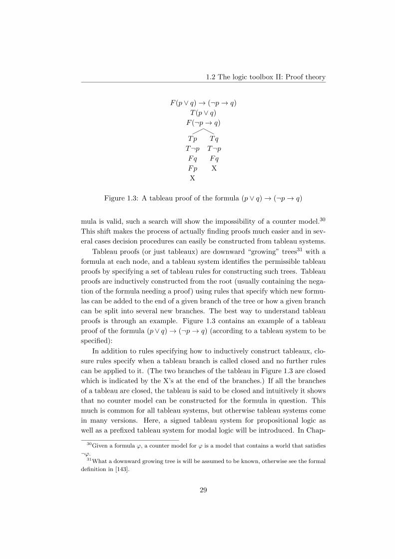
1.2 The logic toolbox II: Proof theory

F (p ∨ q)→ (¬p→ q)

T (p ∨ q)F (¬p→ q)

Tp

T¬pFq

Fp

X

Tq

T¬pFq

X

Figure 1.3: A tableau proof of the formula (p ∨ q)→ (¬p→ q)

mula is valid, such a search will show the impossibility of a counter model.30

This shift makes the process of actually finding proofs much easier and in sev-

eral cases decision procedures can easily be constructed from tableau systems.

Tableau proofs (or just tableaux) are downward “growing” trees31 with a

formula at each node, and a tableau system identifies the permissible tableau

proofs by specifying a set of tableau rules for constructing such trees. Tableau

proofs are inductively constructed from the root (usually containing the nega-

tion of the formula needing a proof) using rules that specify which new formu-

las can be added to the end of a given branch of the tree or how a given branch

can be split into several new branches. The best way to understand tableau

proofs is through an example. Figure 1.3 contains an example of a tableau

proof of the formula (p∨ q)→ (¬p→ q) (according to a tableau system to be

specified):

In addition to rules specifying how to inductively construct tableaux, clo-

sure rules specify when a tableau branch is called closed and no further rules

can be applied to it. (The two branches of the tableau in Figure 1.3 are closed

which is indicated by the X’s at the end of the branches.) If all the branches

of a tableau are closed, the tableau is said to be closed and intuitively it shows

that no counter model can be constructed for the formula in question. This

much is common for all tableau systems, but otherwise tableau systems come

in many versions. Here, a signed tableau system for propositional logic as

well as a prefixed tableau system for modal logic will be introduced. In Chap-

30Given a formula ϕ, a counter model for ϕ is a model that contains a world that satisfies

¬ϕ.31What a downward growing tree is will be assumed to be known, otherwise see the formal

definition in [143].

29

Ch. 1. Introduction

T¬ϕ(T¬)

Fϕ

F¬ϕ(F¬)

Tϕ

T (ϕ ∧ ψ)(T∧)

Tϕ

Tψ

F (ϕ ∧ ψ)(F∧)

Fϕ Fψ

T (ϕ ∨ ψ)(T∨)

Tϕ Tψ

F (ϕ ∨ ψ)(F∨)

Fϕ

Fψ

T (ϕ→ ψ)(T→)

Fϕ Tψ

F (ϕ→ ψ)(F→)

Tϕ

Fψ

Figure 1.4: Signed tableau system for propositional logic.

ter 2 a signed tableau system will be presented for a many-valued hybrid logic

and in Chapter 5 a prefixed tableau system will be given for a hybrid public

announcement logic as well as a logic containing action models.

In a signed tableau system the formulas occurring on the branches of the

tableaux will all be signed formulas of the form Tϕ or Fϕ for formulas ϕ. The

intuition is that Tϕ asserts ϕ to be true, whereas Fϕ asserts ϕ to be false. A

branch is said to be closed if it contains both Tϕ and Fϕ for some formula ϕ,

or if it contains T⊥ or F>. Usually each logical connective gives rise to a rule

involving T and a rule involving F . The tableau rules for propositional logic

are shown in Figure 1.4 (where the connective ↔ has been left out).32

The reading of a rule like (T∧) is that if T (ϕ ∧ ψ) occurs on a branch,

then the two formulas Tϕ and Tψ are both added to the end of the branch.

The reading of a rule like (F∧) is that if F (ϕ ∧ ψ) occurs on a branch, then

the branch is split into two branches, one ending with the formula Fϕ and the

other one ending with the formula Fψ. For a given rule, a formula above the

line is called a premise and a formula below the line is called a conclusion. A

signed tableau proof for a propositional formula ϕ is a closed signed tableau

starting with Fϕ as the root formula. Recall the example of a tableau proof

of the formula (p ∨ q)→ (¬p→ q) given in Figure 1.3.

The presented signed tableau system is not easy to extend to also cover

various modal logics. When dealing with modal logic, prefixed tableau systems

32It is not hard to see that the signs T and F are not really necessary. Tϕ can be replaced

by ϕ and Fϕ by ¬ϕ. The rule (T¬) can then be omitted and a tableau system for unsigned

formulas of propositional logic is obtained. However, the signs make the intuition behind

the tableau rules clear and the signs will also be used for clarity when a tableau system for

a many-valued hybrid logic is presented in Chapter 2.

30

1.2 The logic toolbox II: Proof theory

are better suited.33 The prefixed tableau system introduced now comes from

[37], but it is fairly standard for modal logic. Prefixes are just symbols coming

from a fixed countable infinite set Pref, and σ and τ will normally be used for

elements of Pref. In prefixed tableaux both prefixed formulas σϕ, where ϕ is a

modal formula and σ ∈ Pref, and accessibility formulas σRτ , where σ, τ ∈ Pref,

will occur. The intuition behind the prefixes is that they represent possible

worlds; σϕ represents that ϕ is true in the world σ and σRτ represents that

the world τ is accessible from the world σ.

A branch in a prefixed tableau is said to be closed if it contains both

σϕ and σ¬ϕ for some formula ϕ (note that the prefix σ is the same in both

prefixed formulas). The rules for the prefixed tableau system for standard

modal logic are given in Figure 1.5. The reading of the rules is similar to

the signed tableau system; however, in the rules (�) and (¬♦) there are two

premises which need to be on the branch before the rules are applicable. (The

two premises need not appear in any particular order or be immediately after

each other on the branch though.) Furthermore, the rules (♦) and (¬�) have

a side condition stating that the prefix τ must be a new prefix not already

occurring on the given branch. A prefixed tableau proof for a modal formula

ϕ is a closed prefixed tableau starting with σ¬ϕ as the root formula. The first

tableau system of Chapter 5 is an extension of the tableau system given in

Figure 1.5.

Prefixed tableau systems can be extended to other modal logics much easier

than tableau systems without prefixes, see [62]. When extending the logic to

hybrid logic instead of standard modal logic, tableau systems without prefixes

become feasible for a great variety of other modal logics. This issue will be

discussed further in Section 1.2.2.

As mentioned earlier, tableau proofs are systematic searches for counter

models. Soundness of a tableau system amounts to the fact that all formulas

with tableau proofs are valid, i.e., have no counter model. Then, showing

that all the tableau rules preserve satisfiability (if all the formulas on a branch

are satisfiable then applying any tableau rule will result in at least one new

satisfiable branch) ensures soundness: if a formula is not valid, its negation

is satisfiable and since all tableau rules preserve satisfiability every tableau

starting with the negation of the formula will contain an open branch, and

thus the formula does not have a tableau proof (a closed tableau). Showing

that a tableau rule preserves satisfiability will also be referred to as showing the

33Several prefixed tableau systems for modal logic also use signs such as [62]. However, in

this thesis the prefixed tableau systems will be without signs inspired by [37].

31

Ch. 1. Introduction

σ¬¬ϕ(¬¬)

σϕ

σ(ϕ ∧ ψ)(∧)

σϕ

σψ

σ¬(ϕ ∧ ψ)(¬∧)

σ¬ϕ σ¬ψ

σ(ϕ ∨ ψ)(∨)

σϕ σψ

σ¬(ϕ ∨ ψ)(¬∨)

σ¬ϕσ¬ψ

σ(ϕ→ ψ)(→)

σ¬ϕ σψ

σ¬(ϕ→ ψ)(¬ →)

σϕ

σ¬ψ

σ�ϕ σRτ(�)

τϕ

σ¬�ϕ(¬�)

1

σRτ

τ¬ϕ

σ♦ϕ(♦)

1

σRτ

τϕ

σ¬♦ϕ σRτ(¬♦)

τ¬ϕ

1 The prefix τ is new to the branch.

Figure 1.5: Tableau system for standard modal logic.

soundness of the rule. Often the tableau rules are constructed in such a way

that it is not hard to see that they preserve validity and therefore soundness

is something which will not be discussed much for the tableau systems given

in chapters 2 and 5.

Completeness amounts to showing that every valid formula has a closed

tableau or that every formula for which there exists no closed tableau has a

counter model. Here is a sketch of this way of showing completeness. Assume

that a formula ϕ has no closed tableau. The way to prove completeness is then

to construct a counter model for ϕ, which can be done from an open branch of

a tableau for ϕ. For the open branch to be useful it needs to satisfy a certain

saturation property, which in the prefixed tableau system given for standard

modal logic simply amounts to the requirement that no formulas appear more

than once on the branch, that the rule (♦) has not been applied to the same

formula more than once, and that no more rules are applicable to the formulas

on the branch.34 Completeness of the tableau system of Chapter 2 is basically

shown along these lines, but due to the many-valued setting it is a bit more

involved. In Chapter 5 completeness of the given tableau systems is only briefly

discussed, since it follows more or less straightforwardly from completeness of

34For logics where the tableaux are not ensured to be finite, saturation is usually formulated

a bit differently.

32

1.2 The logic toolbox II: Proof theory

already existing tableau systems. In fact, completeness of the first tableau

system of Chapter 5 follows from the completeness of the tableau system of

Figure 1.5. Completeness of the second tableau system of Chapter 5 follows

from the completeness of a hybrid tableau system, which will be discussed in

Section 1.2.2. The central issue of Chapter 5 is the fact that the given tableau

proofs always terminate, something that can lead to a decision procedure for

the logics.

As mentioned above, tableau systems are useful for designing decision pro-

cedures for logics and thereby showing that they are decidable. The way this

is usually done is by showing soundness, completeness, and termination of

the tableau system. A tableau system is said to be terminating if no infinite

tableaux35 can ever be constructed within the tableau system. How to show

that a tableau system is terminating is discussed in more detail in the next

section, after having introduced hybrid tableau systems. Before a sound, com-

plete, and terminating tableau system can give rise to a decision procedure,

an algorithm needs to be specified, which ensures that tableaux can be con-

structed in such a way that all branches are either saturated or closed. Then,

given a formula of the logic, such a tableau is constructed (which is doable in

finitely many steps due to termination). If the tableau is closed the formula

is valid (due to soundness), if it contains a branch that is not closed, it is also

saturated and the method from the completeness proof shows how a counter

model for the formula can be constructed, which means that the formula is

not valid. This constitutes a decision procedure for the logic.

1.2.2 The proof theory of hybrid logic

How to extend Hilbert-style proof systems as well as tableau systems to hy-

brid logic is discussed in this section. The Hilbert-style proof system to be

presented is the inspiration for the Hilbert-style proof system for the hybrid

public announcement logic given in Chapter 4. The two tableau systems,

which will also be presented, are the inspirations for the tableau system for

the many-valued hybrid logic given in Chapter 2 and the tableau system for

the hybrid public announcement logic given in Chapter 5.

Several Hilbert-style proof systems exist for hybrid logic, but the Hilbert-

style proof system of Chapter 4 is based on a proof system from [28] (also

presented in [8]). The proof system from [28], for hybrid logic with nominals,

satisfaction operators, and the downarrow binder, is shown in Figure 1.6. In

35Here a tableau is said to be infinite if it contains infinitely many nodes.

33

Ch. 1. Introduction

Chapter 4 this proof system is changed somewhat and there are two reasons

for this. Since the aim of Chapter 4 is to combine hybrid logic with public

announcement logic, the substitution rule (subst) has been left out as it is not

valid for public announcement logic.36 Furthermore, in Chapter 4, nominals

are not true in exactly one world but in at most one world, which also forces

a change of the proof system.

Axioms:

All classical tautologies CL

�(p→ q)→ (�p→ �q) K�

@i(p→ q)→ (@ip→ @iq) K@

@ip↔ ¬@i¬p Selfdual@@ii Ref@@i@jp↔ @jp Agree

i→ (p↔ @ip) Intro

♦@ip→ @ip Back

@i(↓s.ϕ↔ ϕ[s := i])1 DA

Rules:

From ϕ and ϕ→ ψ, infer ψ MP

From ϕ, infer ϕσ 2 Subst

From ϕ, infer @iϕ Gen@

From ϕ, infer �ϕ Gen�

From @iϕ, where i does not occur in ϕ, infer ϕ Name

From @i♦j → @jϕ where i 6= j does not occur BGin ϕ, infer @i�ϕ

1 ϕ[s := i] denotes the formula obtained from ϕ by substituting all free occurrences

of s by i. 2 ϕσ denotes the result of substituting formulas for propositional variables

and nominals for nominals according to the substitution σ.

Figure 1.6: The Hilbert-style proof system of [28] for hybrid logic with @ and ↓.

Soundness of the Hilbert-style proof system is proved in the standard way.

Now, however, what is interesting about hybrid logic, and truly makes it a

hybrid between modal logic and first-order logic, is the way to show complete-

ness. This is similar to the way completeness is shown for first-order logic.

Here is a sketch: Given an unprovable formula ϕ, a maximal consistent set

extending {¬ϕ} is built adding “witnesses” for every modal formula ♦ψ in the

form of new nominals, just as witnesses in the form of constants are added

36In public announcement logic [p]p is valid for propositional variables p, but [ϕ]ϕ is not

valid in general.

34

1.2 The logic toolbox II: Proof theory

for existential first-order formulas in the Henkin style completeness proof of

first-order logic.37 Then a model is constructed from the maximal consistent

set taking equivalence classes of nominals as worlds (again just like in the

Henkin construction for first-order logic). Finally, it is shown that a formula

of the form @iψ belongs to the maximal consistent set if and only if ψ is true

in the model at the world consisting of the equivalence class of i. From this it

further follows that the model can be used as a counter model for ϕ. For an

elaboration on this method see Chapter 4.

The new way of showing completeness for hybrid logic has an advantage:

it allows for very general completeness results. A pure formula is a hybrid

logic formula that does not contain any propositional variables. Now, it can

be shown that adding any pure formulas as extra axioms to the proof system

of Figure 1.6 results in a proof system that is automatically complete with

respect to the class of frames the pure formulas define. The class of frames

that a set of pure formulas defines is the class of frames on which they are

valid. With this general completeness theorem, one obtains completeness for

a wide range of hybrid logics since numerous classes can be defined by pure

formulas. The way this general completeness result is shown is quite simple.

Due to a frame lemma it can be shown that, for the model defined in the

completeness proof, the underlying frame always validates all pure formulas

that have been added as axioms, and thus the model constructed is always a

counter model of the “right” kind. In the presence of public announcement

modalities the general completeness results also retain, which is one of the

main results shown in Chapter 4.

The Hilbert-style proof system for standard modal logic is easily extendable

to other modal logics in many cases. This is generally not the case for other

proof systems for modal logic without introducing some extra machinery such

as prefixes, as in the last tableau system of the previous section. However,

for hybrid logic, extra machinery, such as prefixes, is not needed to obtain

nice and uniform proof systems such as tableau systems, natural deduction

systems, or sequent calculus. This is essentially due to the internalization of

the possible world semantics in hybrid logic. For more on the proof theory of

hybrid logic and why it is well-behaved, see the recent book [42].

An internalized tableau system for hybrid logic is a tableau system that

37That nominals can be used as witnesses is not that surprising, once one is viewing hybrid

logic as a fragment of first-order logic and realizes that nominals correspond to constants of

first-order logic, see [8].

35

Ch. 1. Introduction

does not use prefixes, but where prefixes are “simulated” using the satisfaction

operators of hybrid logic. This is done by using formulas of the form @iϕ

instead of σϕ and @i♦j instead of σRτ . In this thesis both prefixed and

internalized tableau systems are considered for hybrid logic. The prefixed

tableau systems for hybrid logic are usually simpler and easier to work with, on

the other hand the internalized tableau systems allow for general completeness

in the same style as for Hilbert-style proof systems for hybrid logic. In [25]

an internalized tableau system is presented and it is shown that it allows for

general completeness by adding the following rule: If H is a set pure formulas,

then any of them are allowed to be added to any tableau branch at any time,

and so are any pure formulas obtained by uniformly substituting nominals for

nominals in formulas of H. [25] then shows that the tableau system with this

additional rule is complete with respect to the class of frames defined by the

formulas in H. However, when extending tableau systems with pure formulas

like this, the tableau system is no longer guaranteed to be terminating.

Terminating tableau systems for hybrid logic have been developed in sev-

eral versions by Blackburn, Bolander, and Brauner in [38, 39, 37, 36]. The

prefixed tableau system of [37] for hybrid logic with nominals, satisfaction op-

erators, and the global modality is shown in Figure 1.7 and is the one extended

to hybrid public announcement logic in Chapter 5. However, since nominals

are true in at most one world instead of exactly one world in the hybrid pub-

lic announcement logic of Chapter 5, the rule (¬) is omitted – which turns

out to be the only change needed. As presented above, the tableau system of

Figure 1.7 is not terminating. An additional loop check condition is needed

that blocks the application of the rules (¬), (♦), (@), (¬@), and (E) based on

properties of the prefix σ. For an elaboration of this see Chapter 5 or [37].

In Chapter 2, prefixes are internalized in the tableau system for many-

valued hybrid logic inspired by the tableau system of [39] shown in Figure 1.8.

However, due to the many-valued setting of Chapter 2 further rules are needed

and the resulting tableau system looks considerably different from the one in

Figure 1.8. Furthermore, signs T and F , as in the tableau system of Figure 1.4,

are also used to simplify the reading of the rules in Chapter 2. Fitting already

gave a signed non-prefixed tableau system in [61] for a many-valued modal

logic. Nevertheless, the great advantage of developing an internalized tableau

for the many-valued hybrid logic is that it can be shown to terminate. It is

not obvious at all how to prove termination of Fitting’s tableau system, if it

is terminating at all.

Soundness and completeness of the hybrid tableau systems, internalized

36

1.2 The logic toolbox II: Proof theory

σ¬i(¬)

1

τi

σ¬¬ϕ(¬¬)

σϕ

σϕ ∧ ψ(∧)

σϕ

σψ

σ¬(ϕ ∧ ψ)(¬∧)

σ¬ϕ σ¬ψ

σ♦ϕ(♦)

1

σRτ

τϕ

σ¬♦ϕ σRτ(¬♦)

τ¬ϕ

σEϕ(E)

1

τϕ

σ¬Eϕ(¬E)

2

τ¬ϕ

σ@iϕ(@)

1

τi

τϕ

σ¬@iϕ(¬@)

1

τi

τ¬ϕ

σϕ σi τi(Id)

τϕ

1 The prefix τ is new to the branch. 2 The prefix τ is already on the branch.

Figure 1.7: The prefixed hybrid tableau system of [37].

@i¬ϕ(¬)

¬@iϕ

¬@i¬ϕ(¬¬)

@iϕ

@iϕ ∧ ψ(∧)

@iϕ

@iψ

¬@i(ϕ ∧ ψ)(¬∧)

¬@iϕ ¬@iψ

@i♦ϕ(♦)

1 2

@i♦j@jϕ

¬@i♦ϕ @i♦j(¬♦)

¬@jϕ

@i@jϕ(@)

@jϕ

¬@i@jϕ(¬@)

¬@jϕ

(ref)3

@ii

@i♦j @jk(Bridge)

@i♦k

@ij @iϕ(Nom1)

4

@jϕ

@ij @j♦k(Nom2)

@i♦k

1 The nominal j is new to the branch. 2 The formula ϕ is not a nominal. 3 The

nominal i is on the branch. 4 The formula ϕ is a propositional variable or a nominal.

Figure 1.8: The internalized hybrid tableau system of [39].

37

Ch. 1. Introduction

or not, are quite similar to soundness and completeness of prefixed tableau

systems. Instead of building the counter model based on prefixes, as in the

completeness for prefixed tableau systems, one builds the counter model based

on the nominals occurring on an open saturated branch, see [37].38 As already

mentioned the many-valued setting of Chapter 2 complicates matters and

the completeness proof presented therein deviates considerably from standard

completeness proofs for hybrid tableau systems. An open saturated tableau

branch does not give rise to a unique counter model anymore, since the tableau

branch only provides lower and upper bounds for truth values. Nonetheless,

it can be shown that any model build from the branch that respects these

bounds, suffices as a counter model.

Termination of tableau systems has been mentioned as an important prop-

erty several times. In the papers [38, 39], Bolander and Brauner developed

a general way of showing termination of tableau systems. It is based on a

non-trivial extension of the idea of showing termination for ordinary tableau

systems for propositional logic. Here it is observed that application of a rule

to a premise of maximal length on a branch always strictly decreases the max-

imal length of formulas on the branch, and thus the maximal length of the

formulas on the branch strictly decreases down along a branch as a rule is ap-

plied. Therefore there can be no infinite branches (since the root formula has

a fixed finite length) and since the tableau is finitely branching it is necessarily

finite. In termination for propositional logic it is also used that no rule can

be applied more than once to a formula, however in modal or hybrid logic the

rule (¬♦) can be used several times due to new prefixes (or nominals) being

introduced on a branch. Instead, one can show that the maximal length of

formulas strictly decreases when moving along the tree constructed from the

new prefixes (or nominals) that are introduced on a branch. In addition it

just needs to be shown that a branch of a tableau is infinite if, and only if,

the corresponding tree of new prefixes has an infinite branch. This method

is exemplified nicely in Chapter 2, otherwise see [37]. The method turns out

to be quite powerful and general, which is shown by this thesis, where the

method is extended both to a many-valued hybrid logic (in Chapter 2) and

dynamic epistemic logics (in Chapter 5).

Exploring the proof theory of hybrid logic has been one of the aims of

38Due to the inclusion of loop check conditions to ensure termination, branches are not

necessarily saturated for all nominals on the branch, but only for a certain kind of nominals,

usually referred to as urfarthers. However, building the counter model from urfarthers alone

suffices for the completeness proof in these cases, see [37].

38

1.2 The logic toolbox II: Proof theory

this thesis; another related aim has been to use the advantages of hybrid logic

proof theory to investigate the proof theory of public announcement logic and

dynamic epistemic logic in general. Therefore, it is time to look closer at the

proof theory of dynamic epistemic logic.

1.2.3 The proof theory of dynamic epistemic logic

Due to the relatively young age of dynamic epistemic logic and the fact that

it has been mostly semantically driven, the proof theory of dynamic epis-

temic logic is somewhat underdeveloped. Furthermore, almost all of the proof

systems for dynamic epistemic logic are Hilbert-style proof systems with the

exception of [14, 49, 117]. This thesis contributes to the proof theory of dy-

namic epistemic logic by giving a Hilbert-style proof system for a hybrid public

announcement logic that allows for automatic completeness with pure formu-

las in Chapter 4, and by giving two terminating tableau systems in Chapter 5,

one for epistemic logic with action modalities and one for the hybrid public

announcement logic of Chapter 4. Therefore this section briefly introduces the

standard Hilbert-style proof systems for dynamic epistemic logic and describes

how completeness can be shown by reduction axioms.

The standard Hilbert-style proof system for public announcement logic

(without common knowledge) is particularly simple, it is obtained by just

adding the reduction axioms (1.1) − (1.5) of Section 1.1.539 to the Hilbert-

style proof system in Figure 1.1 of Section 1.2.1. (If one wants the accessibility

relations to be equivalence relations, one just adds the axioms of S5 for each

agent a ∈ A to this proof system.) Since (1.1) − (1.5) are valid in public

announcement logic, as already mentioned, the resulting proof system is sound.

Completeness of public announcement logic is also easy to obtain, as the

following sketch of the proof shows: First, a translation from public announce-

ment logic to standard modal logic (or epistemic logic) is inductively defined

as in Figure 1.9. It is then shown that for all formulas ϕ of public announce-

ment logic ϕ ↔ t(ϕ) is provable, from which it also follows by the assistance

of the soundness of the proof system that ϕ↔ t(ϕ) is valid. Thus, if a formula

ϕ is valid in public announcement logic, t(ϕ) is also valid. Furthermore, since

the models of public announcement logic and the standard modal logic are

the same, t(ϕ) is also valid in standard modal logic, since t(ϕ) is a formula of

39Note that the reduction axioms (1.2)− (1.5) are axiom schemes, i.e. an axiom is added

for every formula ϕ, ψ and χ, whereas (1.1) is not an axiom scheme, as only propositional

variables are allowed to be substituted for p in (1.1).

39

Ch. 1. Introduction

t(p) = p t([ϕ]p) = t(ϕ→ p)

t(¬ϕ) = ¬t(ϕ) t([ϕ]¬ψ) = t(ϕ→ ¬[ϕ]ψ)

t(ϕ ∧ ψ) = t(ϕ) ∧ t(ψ) t([ϕ]ψ ∧ χ) = t([ϕ]ψ ∧ [ϕ]χ)

t(Kaϕ) = Kat(ϕ) t([ϕ]Kaψ) = t(ϕ→ Ka[ϕ]ψ)

t([ϕ][ψ]χ) = t([ϕ ∧ [ϕ]ψ]χ)

Figure 1.9: The translation t from public announcement logic to epistemic

logic.

standard modal logic. But then, t(ϕ) is provable by the completeness of stan-

dard modal logic. However, because the proof system of public announcement

logic is an extension of the one for standard modal logic, t(ϕ) is provable in

public announcement logic as well, by which it follows by the provability of

ϕ↔ t(ϕ) that ϕ is provable in public announcement logic.

Proving that ϕ↔ t(ϕ) is provable in the proof system is a simple induction

proof. There is one small catch though. The formula complexity does not

decrease every time one step of the translation is performed, and therefore

the induction proof cannot be on the formula complexity as normal. However,

another complexity measure can be defined that strictly decreases for every

step of the translation. The definition of this complexity measure c is shown

below and is taken from [163], where much more on completeness for public

announcement logic is also discussed.

c(p) = 1

c(¬ϕ) = 1 + c(ϕ)

c(ϕ ∧ ψ) = 1 + max(c(ϕ), c(ψ))

c(Kaϕ) = 1 + c(ϕ)

c([ϕ]ψ) = (4 + c(ϕ)) · c(ψ)

The Hilbert-style proof system for public announcement logic does not

always behave that nicely. First of all, the completeness proof and axioma-

tisation just sketched above does not work if common knowledge is added,

simply because no reduction axiom can exist for the combination of the pub-

lic announcement modality and the common knowledge modality, see [163].

Therefore common knowledge is left out in chapters 4 and 5. Secondly, the

Hilbert-style proof system for public announcement logic is not easy to extend

40

1.2 The logic toolbox II: Proof theory

for other frame classes than the class of all frames and the class of equiva-

lence relation frames. For instance, there is a problem with the class of serial

frames (and thereby also the class of frames for KD45) because when moving

to a submodel, as the public announcement modality [ϕ] does, a serial acces-

sibility relation might lose its seriality. This implies that the meaning of a

KD45 belief modality B is different, depending on whether it appears within

the scope of a [ϕ] modality or not.40 This is one of the main reasons that

plausibility models are used when modeling beliefs and public announcement,

which explains the choice of logic in Chapter 6.

A problem of the same kind occurs when one wants to add nominals to

public announcement logic. The semantics of a nominal specifies that it is

true in exactly one world, but if it occurs within the scope of a [ϕ] modality,

that world might have been removed. Fortunately there is a way around this

by letting nominals be true in at most one world both inside and outside the

scope of a [ϕ] modality – this is the approach taken in Chapter 4.

When moving from public announcement logic to dynamic epistemic logic

with action models (and still staying clear of common knowledge) the same way

of defining a Hilbert-style proof system is possible, the reduction axioms (1.6)−(1.10) of Section 1.1.5 are just used instead of the one for public announcement

logic. Completeness and soundness are shown in the same way, a new and

little more complicated complexity measure is needed though. The details are

skipped, but can be found in [163].

When it comes to tableau systems for dynamic epistemic logic, only two

such systems already exist, namely [14, 49], which are both tableau systems for

public announcement logic. These tableau systems are not based on reduction

axioms, but are based on the semantics of the public announcement modality

instead. This allows for the tableau system of [14] to be optimal in terms of

complexity, although it also complicates the rules. Furthermore, due to the

heavy reliance on the specific semantics of the public announcement operator,

there is no obvious way of extending the tableau system of [14] to include

action modalities.

In Chapter 5, tableau systems are given for a dynamic epistemic logic with

action modalities as well as a hybrid public announcement logic. The tableau

systems have very simple rules and are obtained by adding reduction axioms

40This problem is not as much a problem of the proof theory as it is a problem of the

semantics. However, the consequence is that it is not possible to give a sound and complete

proof system for a public announcement logic where the modality B is always interpreted as

a KD45 modality.

41

Ch. 1. Introduction

as rules to the already presented tableau systems of figures 1.5 and 1.7 with the

need of no further rules. It is thereby shown that reduction axioms are useful

in proof theory beyond merely Hilbert-style proof systems. Furthermore, it

allows for the reuse of the soundness and completeness of the tableau systems

of figures 1.5 and 1.7. Finally, the method for proving termination sketched in

the last section can be extended to prove termination of the tableau systems

of Chapter 5 using the new complexity measures.

This concludes a general presentation of the toolbox that the first four

chapters of this thesis extend on. As mentioned, the toolbox can be used for

modeling information, knowledge and beliefs, which will be the subject of the

next sections.

42

1.3 The toolbox at work: modeling information, knowledge, and beliefs

1.3 The toolbox at work: modeling information,

knowledge, and beliefs

After a thorough inventory of the toolbox it is time to put the tools to work.

The tools of the last section have many applications, but here the focus will be

on how they are useful in modeling information, knowledge, and beliefs. These

concepts are widely used in our everyday life as well as in many sciences, re-

sulting in various views on what the concepts mean. However, the focus here

will be on how information, knowledge, and beliefs are viewed and modeled

within philosophy and computer science, more specifically within the subfields

of formal and social epistemology and multi-agent systems. Therefore an in-

troduction to what information, knowledge, an beliefs signify in these fields

will be given in Section 1.3.1. Within these fields logic has turned out to be

a useful tool in modeling and clarifying the concepts. Why this is the case is

discussed in Section 1.3.2, where the topics of the chapters 6 and 7 are also

put in a greater context. Finally, in Section 1.3.3 a possible future application

of the logic introduced in Chapter 2 is discussed.

1.3.1 Information, knowledge, and beliefs in philosophy and

computer science

Information is an important part of our life. From bombing the right troops

to catching a train to work, the proper information is central to making the

right decisions. In our increasingly specialized and fast-moving society some

decisions require increased amounts of expert knowledge and others require

great coordination among several agents - both humans, computer programs,

and robots. This only makes information and how we handle it even more

important; so important that we talk about “the information age”.

Moreover, the amount of information we produce and store as a human

society is vastly increasing due to modern technology. The telecommunica-

tion and IT industry in Denmark is estimated to have made 550,000,000,000

registrations of phone calls and internet traffic last year (due to the Danish

anti-terror law) [171], and the laws regarding unemployment benefits in Den-

mark now comprise 22,575 pages of rules [120]. It is estimated that humanity

had accumulated 12 exabytes of information in 2003 and this passed 988 ex-

abytes in 2010, which makes the philosopher Luciano Floridi talk about the

“zettabyte era”41 [66].

411 exabyte equals 1018 bytes and 1000 exabytes equals 1 zettabyte.

43

Ch. 1. Introduction

It seems obvious that information is important, while at the same time

providing the human race with great challenges. However, what does infor-

mation really amount to? Compared to the long history of philosophy it is

only recently that information has received profound attention within the field,

actually, philosophy of information has now become an independent subfield,

[2, 65, 67]. On the other hand, what has received great attention in philosophy

since ancient times, is the concept of knowledge. In decision-making the right

information is vital, but it is only useful if the acting agents possess the infor-

mation and they trust it enough to act upon it. It is not as much information

we base our decisions on, as it is our knowledge.42

1.3.1.1 Epistemology

Epistemology is the subfield of philosophy mainly dealing with knowledge,

especially the question of what it amounts to for an agent to have knowledge of

a proposition43. Traditionally, going back to Plato, knowledge has been defined

as justified true belief. For an agent to know that ϕ, ϕ needs to be true, the

agent must believe ϕ, and the agent must be justified in believing ϕ. However,

this view was shaken by Gettier’s short paper [71] in 1963 that presented two

counter examples to the “justified true belief” analysis of knowledge, which

showed that justified true belief in a formula ϕ can be ascribed to a person

without the person having knowledge of ϕ.

Conventionally, epistemology has mainly focused on analyzing what knowl-

edge or justification amount to, avoiding the Gettier examples, or argued for or

against the mere possibility of knowledge. The role of knowledge in decision-

making has been left for other disciplines, though, some philosophers, such

as Hintikka ([97], chapter 1), have noted the strong ties between knowledge

and decision-making. Furthermore, the precise relationship between knowl-

edge and information is something which is open for discussion.44 The reason

42This is of course open to philosophical debate, something which will be ignored here to

keep the introduction focused.43Knowledge in the form of “knowing how to...” has received little attention within main-

stream epistemology.44According to Luciano Floridi [66] the general definition of information states that in-

formation is meaningful, well-formed data and that semantic information is well-formed,

meaningful, and truthful data. He further claims that information can give way to knowl-

edge, in the sense that knowledge relates and justifies semantic information [66]. However,

the relation to the traditional analysis of knowledge remains vague. Furthermore, this is just

one view on the relation between knowledge and information, and several others are possible

– once again, a detailed philosophical debate that will lead this introduction astray.

44

1.3 The toolbox at work: modeling information, knowledge, and beliefs

for bringing in epistemology is that it clearly relates to epistemic logic (as

introduced in sections 1.1.4 and 1.1.5 and being the concern of chapters 4, 5,

and 6). Even though Hintikka introduced epistemic logic into epistemology

in 1962 [96], epistemic logic and mainstream epistemology have lived separate

lives [90]. This, however, is now changing mainly due to the new subfields of

formal epistemology and social epistemology.

1.3.1.2 Formal epistemology

Broadly viewed, epistemology now deals with knowledge, belief (-change), cer-

tainty, rationality, reasoning, decision, justification, learning, agent interac-

tion, and information processing. On such a view, formal epistemology con-

siders the same topics as mainstream epistemology, but attacks them with

formal mathematical tools such as logic, probability theory, game theory, de-

cision theory, formal learning theory, belief revision, or distributed computing

[89]. There is no doubt though that formal epistemology and mainstream epis-

temology have focused on quite different aspects of knowledge. For instance,

in belief revision and dynamic epistemic logic, the focus in not on an adequate

definition of knowledge as in mainstream epistemology, but on how knowledge

and information change (or should change) as a result of new incoming in-

formation or changes in the world. However, there is nothing to hinder the

two approaches getting together and learning from each other. Viewing main-

stream and formal epistemology as being on the same quest is advocated by

Vincent Hendricks in [90], for instance. Even though logic is just one of many

tools put to work by formal epistemology, there is no doubt that it will continue

to be a valuable part of the formal epistemology toolbox. Especially epistemic

logic now plays a role in formal epistemology, see for instance [90, 93, 149].

There are several trends in the recent development of epistemic logic that

has brought it closer to philosophy. For one, the dynamic turn in epistemic

logic, most strongly advocated by Johan van Benthem [153], has revolutionized

epistemic logic and among other things resulted in the many applications men-

tioned in Section 1.1.5. The dynamic turn in epistemic logic has emphasized

the issue of how knowledge changes, or more generally of how information flows

under actions such as observation, inference, or communication [152]. In [150]

Johan van Benthem even claims that “...information cannot be understood in

isolation from the processes which convey and transform it. No information

without transformation.”

The new logics developed under the dynamic turn possess increased ex-

45

Ch. 1. Introduction

pressive powers to formalize discussions within mainstream epistemology. For

instance, several versions of the view that knowledge is belief that is stable un-

der belief revision with any new evidence, have been formalized and compared

by Alexandru Baltag and Sonja Smets in [17]. The epistemic logics introduced

in chapters 4 and 5 of this thesis are dynamic epistemic logics, and moreover

the logical framework of [17] is used in Chapter 6 to formalize the phenomenon

of pluralistic ignorance and thus, this thesis embraces the dynamic turn.

Pluralistic ignorance is a phenomenon from social psychology, where a

group of people does not believe something to be the case, but believe that

everyone else in the group believes it to be the case. The phenomenon is

explained in much more detail in Chapter 6 and is also briefly discussed in

Section 1.3.2.3. One essential feature of the phenomenon is that it is a genuine

social phenomenon – no single person and his beliefs can constitute pluralis-

tic ignorance. To capture the fact that the phenomenon involves more than

one person, logics incorporating several people or agents are required. The

interaction between several agents has also turned out to provide a valuable

model of computation leading to the field of multi-agent systems. However,

before saying more about multi-agent systems, it is worth elaborating how the

“many agents” view has also emerged in epistemology.

1.3.1.3 Social epistemology

The focus on knowledge in the context of several individuals has led to the

branch of philosophy called social epistemology. Goldman, in [75], distin-

guishes between three different ways that epistemology can be “social”. The

first way runs close to mainstream epistemology and acknowledges the fact

that epistemic agents are often present in a social reality that affects the way

the agents may gain and handle knowledge. For instance, we repeatedly gain

knowledge through testimony from others in our everyday life. A typical ques-

tion here would be whether beliefs obtained through testimony are justified,

a question that fits well with the practice of mainstream epistemology.

Another way epistemology could be social is by going beyond individual

agents and considering collective agents, such as juries, agencies, corporations

etc. (Such collective agents contain individual agents though.) There are

several examples from daily life where we ascribe knowledge and beliefs to

such collective agents, for instance: “the CIA knew where Osama bin Laden

was hiding”, “the jury believes that the accused is guilty”. The question of

what a collective agent may come to know or believe has received increased

46

1.3 The toolbox at work: modeling information, knowledge, and beliefs

attention lately and has fostered the study of judgment aggregation. Judgment

aggregation mainly uses formal tools to study how a collective agent can form

a judgment based on the judgments of the individual agents it consists of.

Judgment aggregation will be discussed in more detail in Section 1.3.3 since

it provides a possible future application of the logic introduced in Chapter 2.

The third way that epistemology can be “social” is through the study of

what Goldman [75] calls epistemic systems. Collective agents can be epistemic

systems, but epistemic systems go beyond mere collective agents. Goldman

mentions science, education, and journalism as examples of epistemic systems.

For more on this system-oriented social epistemology see [75].

The study of a phenomenon such as pluralistic ignorance can be regarded

as social epistemology to the extent that the phenomenon can be viewed as

an informational phenomenon. If this is the case, the study will involve as-

pects of the first two versions of social epistemology. First of all, pluralistic

ignorance can be seen as a phenomenon where a collective agent holds a belief

that conflicts with the individual agents. Secondly, exactly how information

flows between different agents in a case of pluralistic ignorance and affects the

agents’ individual beliefs is something that is certainly worth studying.45

One of the key features of pluralistic ignorance is the fact that people are

holding wrong beliefs about other people’s beliefs. In the classical account,

one thing that distinguishes beliefs from knowledge is the fact that beliefs can

be wrong, whereas knowledge cannot. Thus, a logic-based model of pluralis-

tic ignorance requires focus on beliefs instead of knowledge, and it therefore

provides a nice example of why it is sometimes useful to shift focus from knowl-

edge to beliefs. What exactly beliefs are is of course also open to philosophical

discussion, see [137]. As for knowledge, belief is viewed as a propositional at-

titude, that is, it is a mental state of having some attitude, stance, or opinion

towards a given proposition [137]. Viewing knowledge and beliefs this way

makes it natural to approach epistemic or doxastic logic in a modal logic way,

as in Section 1.1.4. For an overview of other formal approaches to modeling

beliefs see [101]. Here it will just be noted that in the usual logic-based mod-

eling of beliefs, the key feature that distinguishes it from knowledge is the lack

of veridicality, that is a belief in ϕ does not imply the truth of ϕ as is the

case for knowledge. However, beliefs are required to be consistent, that is an

agent cannot both believe ϕ and ¬ϕ for some formula ϕ. In terms of Kripke

semantics, the accessibility relation underlying the belief modality is required

45In fact, pluralistic ignorance in one of the four central topics in the ongoing series of

workshops in social epistemology between Copenhagen and Lund [92].

47

Ch. 1. Introduction

to be serial instead of the stronger requirement of being reflexive, as required

for knowledge.

1.3.1.4 Multi-agent systems

The advancement of computer science and the internet has made a vast amount

of information easily available to us, but it has also contributed to a huge

expansion in the total amount of information. The increased amount of infor-

mation makes it still harder to find the right information. Furthermore, we

need to communicate the information to a greater extent across several differ-

ent contexts (patients’ information needs to be available to patients, doctors,

nurses, lawyers, employers, and public services). Thus, tools that can help

us find, understand, manage, and communicate information automatically on

larger scales are an enormous advantage. The great increase in information

is made possible due to the development of computers, and the majority of

computer scientists are focused on handling this information challenge. The

field multi-agent systems has grown out of computer science and deals with

information, knowledge and beliefs in several ways.

Multi-agent systems is a relatively new and fast growing subfield of com-

puter science that approaches the increased complexity and size of computer

systems in a novel way. In the multi-agent paradigm, computer systems are

assumed to be composed of autonomous agents that constantly make deci-

sions on which actions to take in pursuit of their individual goals within an

environment. In deciding which actions to adopt, the agents need to consult

their propositional attitudes such as knowledge, beliefs, preferences, and inten-

tions. Furthermore, since the agents often have to communicate, cooperate,

coordinate, and negotiate with each other, they also need to reason about

other agents’ propositional attitudes. Thus, it seems obvious that the field of

multi-agent systems has many overlaps with philosophy, especially social epis-

temology and logic, as well as economics, especially game theory. In general,

the multi-agent view on computing is inspired by other fields, such as logic,

philosophy, economics, psychology, sociology, and linguistics that use similar

agent-based models. Thus, interest in systems of interacting agents spans over

a greater scientific community.

There is no unified definition of what a multi-agent system is, however,

there are several key features (for more see [172]):

• Multi-agent systems are made up of autonomous agents. This is in con-

trast to agents that are told what to do in every situation and thus in a

48

1.3 The toolbox at work: modeling information, knowledge, and beliefs

multi-agent system there is no central agent in control of the system.

• Agents may be equipped with goals and preferences that guide their de-

cisions and allow them to act on behalf of their creator or whoever owns

them.

• Agents are not omnipotent and are not situated in a static environment.

Agents are situated in a dynamic environment with other agents with

whom they can interact through communication, cooperation, coordi-

nation, and negotiation and thereby increase their chances of achieving

their goals.

The first two features reflect the fact that agents in a multi-agent system

behave intelligently, which is the reason why the field of multi-agent systems

is closely related to the field of artificial intelligence, which goes back to Mc-

Carty’s in the 1950s [147]. However, one major feature that distinguishes

multi-agent systems from artificial intelligence is the inclusion of the third

feature mentioned above. A key feature of multi-agent systems is that the

agents are situated in an environment of other agents, or put differently that

they are always members of an agent society. Hence, whereas artificial in-

telligence studies intelligent agents, multi-agent systems studies systems of

intelligent agents.

Examples of multi-agent systems and agents are plentiful. For instance,

[57] mention the following examples of agents: “negotiators in a bargaining

situation, communicating robots, or even components such as wires or mes-

sage buffers in a complicated computer system”. Furthermore, due to the

advancement of the internet, most modern software is required to deal with

autonomous interacting processes, which makes the multi-agent paradigm im-

mensely appealing.

In addition to the fact that agents are situated in an environment of other

agents, they usually also only have limited information. In other words, agents

are typically not omniscient; they have local views of the world and thus only

possess partial knowledge of the world. In this way they resemble real human

agents. The resemblance with human agents also reveals the usefulness of

knowledge and information: we know from our everyday life that information,

knowledge, and beliefs play an important role in corporation, coordination,

and negotiation. The same is the case in multi-agent systems. [57] provides

additional examples of how reasoning about knowledge plays a role in multi-

agent systems. Thus, it may come as no surprise that logics that deal with

knowledge and beliefs are useful in multi-agent systems.

49

Ch. 1. Introduction

Because of the social aspect of multi-agent systems, communication among

agents plays an important role. However, for communication to be possible

between artificial agents, they need to speak a common language. By a com-

mon language, more is meant than just agents sharing a syntax, they also

need to share a semantics – they need to be talking about the same things.

This is one motivation for the development of common semantic frameworks,

such as formal ontologies, which specifies a set of terms used to talk about

a domain [172]. An example is the medical ontology SNOMED CT (System-

atized Nomenclature of Medicine-Clinical Terms), which is a collection of over

311,000 structured medical terms with meaning [102]. Moreover, ontologies,

and ontology languages such as OWL, are heavily involved in the idea of the

semantic web, namely that information on the internet should be equipped

with “meaning”, see [100]. In addition to being a necessity for communica-

tion, the search for common semantic frameworks is the concern of “knowledge

representation and reasoning”, usually regarded as a subfield of artificial in-

telligence. The ability to represent vast amounts of knowledge in a way that

is understandable by many and easy to access, is an advantage that goes well

beyond applications in multi-agent systems. A standard example is the de-

velopment of electronic patient files within healthcare. Due to the enormous

quantity of concepts in the medical world and the fact that doctors, nurses,

pharmacists, etc. may all use the concepts differently, it is an example with

great complexity as well as large potential benefits.

The task of forming common semantic frameworks to make communication

possible is something currently not discussed in social epistemology. However,

it is a prerequisite for the exchange of information in a society, and therefore

it deserves more attention within the social epistemology community. Nev-

ertheless, philosophers are showing increased interest in constructing formal

ontologies, especially in connection with biomedical sciences as exemplified by

the collection [121]. For more on the relation between ontology in philosophy

and computer science see [142]. How logic is used for knowledge representation

through ontologies is further discussed in Section 1.3.2.1.

Another common problem in multi-agent systems is the need for agents

to aggregate their preferences, judgments, beliefs, etc. [3]. For instance if a

set of agents needs to coordinate an action, they need somehow to agree on

taking that action. One such way of coming to agreement is through voting.

Another example is an agent receiving different information from different

sources who has to make up his mind on what to believe. Finally, the problem

of judgment aggregation is yet another example where agents need to aggregate

50

1.3 The toolbox at work: modeling information, knowledge, and beliefs

their judgment on some propositions.

A final note on the relationship between social epistemology and multi-

agent systems is in order. Viewing social epistemology as being only about

human agents and viewing multi-agent systems as being only about artificial

agents makes the two fields disjoint. However, these are narrow views of the

fields and in reality the two fields deal with many of the same topics and

even use the same methods cf. the problem of judgment aggregation. Overall,

information, knowledge, and beliefs are concepts that play a key role in both

disciplines and moreover, they share a logic toolbox to model these concepts.

As previously mentioned, the need for tools that can help us find, under-

stand, manage, and communicate information automatically on larger scales

is great. Logic is a tool that through multi-agent systems can help in this pro-

cess as, for instance, it allows for a better structuring of information through

knowledge representation, for retrieval of new information through automated

theorem proving, and for verification of information handling systems. Fur-

thermore, logic may help clarify concepts related to information, knowledge,

and beliefs, as they are discussed in epistemology. A more detailed discussion

of the usefulness of logic in modeling information, knowledge, and beliefs is

the topic of the next section.

1.3.2 Logic-based modeling of information, knowledge, and

beliefs

Information plays a role in almost every science. However, when it comes to

actual theories of information, Shannon’s Mathematical Theory of Communi-

cation, dating back to [138], seems to be the first. Since then many different

theories of information have emerged and existing theories have incorporated

information as an important concept, most of them are described or men-

tioned in [2]. There is currently no unified theory of information, even though

the different theories have much in common. Information seems such a broad

concept that no unified theory is lurking around the corner. Using the ter-

minology of [1], the different theories can be divided into large-scale views of

information, such as in physics, kolmogorov complexity, or Shannon informa-

tion theory, and small-scale views of information, regarding questions such as

how individual agents possess, handle, and exchange information. Logic as a

theory of information mostly regards the small-scale view [1].

Information shows itself in many forms in logic. The most direct form is the

one it takes in epistemic logic. In epistemic logic agents explicitly reason about

51

Ch. 1. Introduction

knowledge (and beliefs) and since knowledge involves information, epistemic

logic certainly deals with information. The way epistemic logic deals with in-

formation is by viewing it as “range”, to use the word of Johan van Benthem

[1, 155].46 As mentioned in Section 1.1.4, the “information as range” view

is exemplified in epistemic logic by the definition of knowledge: ϕ is known

to an agent if ϕ is true in all the worlds the agent considers possible. If an

agent receives new information and thereby gains new knowledge, then the

set of worlds he considers possible is decreased – i.e. information gain equals

a shrinking of the “range”. Thus, knowledge is defined explicitly in epistemic

logic, and the same goes for beliefs (whether or not one uses plausibility mod-

els to define beliefs). Epistemic logic has another advantage when it comes

to modeling knowledge, which is the fact that higher-order knowledge is eas-

ily dealt with. How epistemic logic allows for reasoning about higher-order

knowledge and why it is useful in modeling knowledge, beliefs or information

will be returned to in Section 1.3.2.3.

Another place where information shows up within logic is in connection

with the syntactic or proof theoretic aspects of logic. A proof system for a

logic takes syntactic input in the form of formulas and outputs new formulas

that follow from the input without involving the semantics of the formulas.

This can be viewed as a way of extracting some of the information contained in

the premises [155]. Alternatively it can be viewed as a way of obtaining new in-

formation from already given information (expressed by the premises). These

are two different views on the informativeness of deduction. The question of

whether deductions produce new information or not is a deep philosophical

question also known as the paradox of deduction or the scandal of deduction

[66]. In one sense deduction seems to convey no new information that is not al-

ready contained in the premise, since the conclusion of a deduction follows with

logical necessity from the premises. However real-life cases, where deduction

provides new information, are plentiful. When it comes to computationally

bounded agents such as humans or computers, deduction can indeed be useful

and seems to be able to provide new information. We will not go into the

philosophical discussion of the paradox of deduction, but merely notice the

usefulness of deduction, at least for resource-bounded agents. The usefulness

46The “Information as range” view can be generalized beyond epistemic logic. In a given

logic specified with respect to a semantic, the information contained in a formula can be

viewed as the class of models that satisfies it, [155]. Thus, gaining information corresponds

to decreasing the class of models, just as gaining information corresponds to eliminating

possible worlds in epistemic logic.

52

1.3 The toolbox at work: modeling information, knowledge, and beliefs

of (automated) deduction will be further discussed in Section 1.3.2.2.

The reason why information is useful is because it is about something

[66]. Focusing on the aboutness of information, [155] mentions yet another

way where information shows up within logic, namely in situation theory.

Here information is viewed as correlation. A situation can carry information

about another situation because there is a correlation between the situations.47

Keeping focus on the aboutness of information, there is another aspect of

logic that deals with information which is not mentioned in [155]. This is the

fact that logic is highly useful in structuring information – logical languages

are exceptionally convenient for representing knowledge. A merely syntac-

tic language cannot be used to represent information without the aboutness

getting lost; the language needs to be accompanied by semantics. However,

logic deals with developing formal languages with associated semantics and

is thereby ideal for representing knowledge. Furthermore, as previously dis-

cussed, a common language is a prerequisite for successful communication or

transfer of information. This requires an agreement of the used terms and

once again the formal languages of logic are useful. The usefulness of logic in

structuring information will now be elaborated.

1.3.2.1 Structuring information in formal ontologies

The importance of representing domain knowledge in a formal language, both

for storing information as well as for making communication possible, should

be clear by now. From the section introducing description logic (i.e. Sec-

tion 1.1.3) it might also be obvious how a logic like description logic is useful

in representing domain knowledge. Still, it is appropriate in the light of Chap-

ter 7 to go into more detail on these matters.

Representing knowledge can be done, and has been done, in many ways

within computer science as witnessed by the large field “knowledge represen-

tation and reasoning”. One way to represent knowledge is through ontologies,

and especially formal ontologies have received great attention within computer

science. There is no agreed, concise definition of what an ontology is, however,

the following comes close; an ontology is a specification of a collection of terms

and relations between them used to describe a particular domain, or with the

words of [77]: “An ontology is an explicit specification of a conceptualization”.

For ontologies to be implemented in computer systems they need to be made

47Viewing information as correlation and as range can be combined in a epistemic logic

about situations, see [155].

53

Ch. 1. Introduction

formal, i.e. they need to be specified in a formal language, which again can

be done in several ways. One widespread formal language, especially devel-

oped for the semantic web, is OWL [100]. Another way to specify an ontology

is to use a formal logic such as description logic.48 From the viewpoint of

description logic, an ontology is simply a TBox.49

In line with the semantics of description logic, the world can be viewed

as consisting of individuals (or instances), concepts (or classes) of individuals,

and relations between individuals. An individual like a person Mary can be an

instance of the concept Woman and stand in a special relation has mother to her

mother Ann, expressed in description logic as has mother(Mary,Ann). Now, the

class Woman is a subclass of the class of persons, expressed in description logic

as Woman v Person. Furthermore, the class Person has the special property

that every one of its members stands in the has mother relation to at least

one person (actually exactly one) who is a woman, which again in description

logic can be expressed as Person v ∃has mother.Woman. Thus, the formula

Person v ∃has mother.Woman expresses a relationship between the two classes

Person and Woman, and so does Woman v Person. Such relationships between

classes are also referred to as class relations.

Ontologies are becoming increasingly important for the biomedical sciences

since the vast amount of information they deal with can be systematized in

large formal ontologies. Again the medical ontology SNOMED CT is an illumi-

nating example, which as previously mentioned has more than 311,000 unique

concepts and approximately 1,360,000 relationships between concepts [102].

For instance SNOMED contains the concept Hepatitis, which in description

logic syntax is defined by ([136]):

Hepatitis ≡ Inflammatory disease u ∃has location.Liver

With the enormous size of SNOMED CT the possibility of contradictions

arising every time changes are made to the ontology is quite likely. For this

reason, before releasing a new version of SNOMED CT, a description logic

reasoner is used to check that the ontology remains consistent. Furthermore,

in local applications of SNOMED CT new concepts may need to be added.

48The standard syntaxes of description logic and OWL are different, however, one version

of OWL, namely OWL DL, has been made to correspond exactly to description logic. Thus,

the difference between using OWL and using description logic is not so important.49Since there is no agreed definition of what an ontology is, it is possible to view an

ontology as also consisting of an ABox, however, viewing an ontology as only being a TBox

seems to be the common view, where the union of a TBox and an ABox are usually referred

to as a knowledge base.

54

1.3 The toolbox at work: modeling information, knowledge, and beliefs

When defining a new concept into the ontology it is possible that the new

concept will have derived properties not explicitly given by the definition.

Due to the size of the ontology, the only way to find out if this is the case is

through automated reasoning using a description logic reasoner for instance.

The tasks of checking whether SNOMED CT is consistent, finding derived

properties of new concepts, as well as computing the entire subsumption hier-

archy of SNOMED CT are examples of the description logic reasoning tasks

described in Section 1.1.3. In addition, description logic can be used to infer

new relationships between classes that may not be explicitly known to anyone

yet.50

There are apparently great advantages in using logic to deal with large

ontologies. However, before logic can be put to work, a formal ontology repre-

senting the domain needs to be constructed. This, in itself, can be a difficult

task. One job that can obviously take a great deal of work is to collect all

the information that needs to go into the ontology. Nevertheless, before this

can be done at all, the domain in question needs to be clarified to such an

extent that a formal language like description logic or OWL can be used to

represent knowledge of the domain. Clarifying the domain and tailoring in

detail a formal language to be able to describe interesting knowledge about a

domain, is something that can require intensive philosophical consideration.

However, the more expressive and precise our language is in talking about

some domain, the easier it is to represent, obtain, and communicate useful

information about the domain. Ideally, electronic patient journals will con-

tain useful information in the sense that not only doctors, nurses, and other

medical staff at the hospital can all understand it, but also doctors, nurses

etc, at other hospitals and in other countries, so that they too can deliver the

right treatment for the patient.

In Chapter 7 such philosophical considerations are applied to the domain of

regulatory relations, especially as they appear in biomedical pathways. Regu-

latory relations are viewed as relations between classes such as in the statement

“insulin positively regulates glucose transport”. Usually when representing re-

lations between a class C and a class D, one of the following two formulas of

description logic is used:

C v ∃R.D or C v ∀R.D.50Description logic is extremely useful when dealing with a large ontology such as

SNOMED CT, however, it is possible to use other logics to reason about an ontology such as

SNOMED CT. Still, description logic remains one of the dominating logics to reason about

formal ontologies.

55

Ch. 1. Introduction

However, based on philosophical considerations and specific domain knowl-

edge, it is argued in Chapter 7 that none of these adequately represent regula-

tory class relations. Instead first-order logic is used and the chapter discusses

how to extend classical description logics to capture regulatory class relations

as well.

1.3.2.2 Automated reasoning

Logic aims at creating formal models of reasoning to distinguish “correct”

reasoning from “wrong” reasoning. Proof theory then provides methods for

determining whether an argument constitutes correct reasoning, as discussed

in Section 1.2. Furthermore, in numerous cases, the determination of correct

reasoning can be automated to such an extent that computers can be pro-

grammed to do the job. (For undecidable logics such programs are not guar-

anteed to give an answer to every input, of course.) In general, automated

reasoning is the study of computer-assisted reasoning.

The significance of automated reasoning when dealing with ontologies and

knowledge representation was discussed in detail in the last section; however,

automated logic reasoning is useful in various other areas. In this section,

other uses of automated reasoning are briefly discussed and connections are

made with the proof theoretic issues presented in Section 1.2.

Disciplines where automated reasoning is widely used include specification

and verification of hardware and software systems. Formal verification of hard-

ware systems is used in industry, for instance to ensure that microprocessors

work correctly, whereas formal verification of security protocols is an example

of software verification. Hardware as well as software systems play essential

roles in numerous activities, however, the complexity of such systems increases

the likelihood of errors occurring in the systems. To avoid such errors, systems

can be formally verified to meet their design specifications and thereby exclude

the possibility of errors. A specification is a description of some desirable prop-

erties of a system, whereas a formal verification (or a proof of correctness) of

a system is a formal mathematical proof that the system actually satisfies the

required specifications. However, for such a formal proof to be possible, the

specifications need to be properly presented in the same formal language as

the proof is to be carried out in. Correctness of programs and hardware can

only be verified with respect to a given specification – to answer the question of

whether a program behaves correctly we need to have specified formally what

it means for a program to “behave correctly”. Note that a specification does

56

1.3 The toolbox at work: modeling information, knowledge, and beliefs

not specify how a system should be designed to obtain its desirable properties

– this is a completely different story.

Logic provides several formal languages to represent specifications as well

as a rich proof theory to find such formal proofs. Nevertheless, the “proofs”

of proof theory are not the only way to provide formal proofs of correctness of

systems, model checking can be used as well – a system can be abstracted to

a model of a particular logical language in which the specifications are stated,

after which it can be checked whether the model satisfies the specifications.

Either way, logic has shown itself useful in specifying and verifying software

and hardware systems which include multi-agent systems [172].

As mentioned in Section 1.1.5 dynamic epistemic logic has been used for

verification of security protocols for communications in multi-agent systems

[164, 50, 51, 95, 4]. For instance, [164] use dynamic epistemic logic for auto-

matic verification of anonymity in security protocols. Specification of protocols

in multi-agent systems was also discussed in the standard reference [57]. [51]

provides an overview of the use of epistemic logic in the analysis of security

protocols. See [172, 166] for other examples of the use of automated reasoning

and logic in specification and verification of multi-agent systems.

It is beoynd the scope of this thesis to design automated reasoning systems

for the introduced logics, however, the work of chapters 2 and 5 are first steps

towards automatic reasoning. Chapters 2 and 5 provide terminating tableau

systems for three logics, and at the end of Section 1.2.1 it was sketched how

such terminating tableau system can give rise to decision procedures. Even

though such decision procedures are an important steps towards automated

reasoning for the given logics, there is the non-trivial task of implementing

the decision procedures. Implementing the decision procedures resulting from

the tableau systems of chapters 2 and 5, is beyond the scope of this thesis.

Nevertheless it should be mentioned that the tableau systems of [37] discussed

in Section 1.2.2 have been implemented in for example the HTab theorem

prover [98]. Hence, implementation of the tableau systems of chapters 2 and

5 might be done as extensions of HTab.

An implemented decision procedure is not a final objective for automated

reasoning in itself. If a decision procedure is implemented, an answer to the

question of validity of a formula is guaranteed, however, the answer might

not be provided in a short time, it might even take longer than the time the

universe is expected to exist. This leads to the issue of tractability, and the task

of optimizing implementation to make it more tractable. However, there might

be a theoretical bound on how much optimizations can be achieved, coming

57

Ch. 1. Introduction

from the computational complexity of a logic. Such issues are important and

intensely studied, but beyond the scope of this thesis as well.

As observed, there are several issues to consider when developing auto-

mated reasoning, and other proof systems than tableau systems can be the

starting point as well – tableau systems are not the only way or always the

best way necessarily. Furthermore, model checking is another important task

for automated reasoning. In general, automated reasoning is a large field that

tackles several important issues not discussed here and uses a variety of other

advanced methods. Still, automated reasoning has many applications in com-

puter science beyond the already mentioned applications in formal ontologies

and knowledge representation as well as the applications in specification and

verification of hardware and software systems. In addition, automated rea-

soning has applications in philosophy and mathematics as well. See [129] for

a general introduction to automated reasoning as well as further applications.

1.3.2.3 Reasoning about knowledge about knowledge about...

Knowledge or information is important for agents when deciding which actions

to adopt. However, knowledge about other agents’ knowledge can also be

important in a multi-agent setting when agents have to cooperate, coordinate,

and negotiate. In this section the importance of reasoning about other agents’

information, knowledge, and beliefs is elaborated further.

Computer science contains numerous examples of the usefulness of reason-

ing about knowledge. For instance, in security protocols for communications

in multi-agent systems, a receiver reasons about whether a sender knows that

he knows the content of the message. Another related example is the Rus-

sian card problem [161, 163], which shows the importance of correct reasoning

about other agents’ knowledge in designing cryptographic protocols. In the

Russian card problem seven cards (denoted by 0, 1, 2, 3, 4, 5, 6) are distributed

between three agents a, b, and c, such that a receives 3 cards, b receives 3

cards, and c receives the final card. The problem is now to design a protocol

specifying how agent a and b can inform each other about their own cards

through truthful public announcements (also perceivable by c) in such a way

that afterwards a knows all of b’s 3 cards, b knows all of a’s 3 cards, and c

knows none of a’s or b’s cards.51 Assume that actually a has cards 0, 1, 2 and

b has cards 3, 4, 5. If a announces that “I have 0, 1, 2 or b has 0, 1, 2” and b

51It is assumed common knowledge that all agents know that a has 3 cards, b has 3 cards,

c has 1 card, and all the cards are among the cards 0, 1, 2, 3, 4, 5, 6.

58

1.3 The toolbox at work: modeling information, knowledge, and beliefs

afterwards announces that “I have 3, 4, 5 or a has 3, 4, 5”, it might seem that

the problem has been solved, however, the first announcement can only be

made safely by a if she has 0, 1, 2, which c can use to learn that a has 0, 1, 2,

[163]. The non-trivial insight that this does not constitute a solution can be

made clear with a formalization of the problem and the solution into dynamic

epistemic logic, see [161, 163]. Thus, dynamic epistemic logic is a powerful

formalism to represent reasoning about knowledge.

Another classic example is the Muddy children puzzle (see for instance

[57, 163]): A group of n children have been playing outside in the mud and

k ≥ 1 of them have become muddy on their forehead. The children can see the

mud on the other children’s forehead, but they cannot see whether they have

muddy foreheads themselves. The father then announces to them that at least

one of them is muddy. He then asks all of those who know they are muddy

to step forward. If no one steps forward, he repeats his request. As long as

none of the children step forward he keeps repeating the request in this way.

If the children are all perfect logical reasoners all the muddy children will step

forward after the father has repeated the request k times. Again, this can be

modeled in epistemic or dynamic epistemic logic, see [57, 163]. In this example

it is essential that the children reason about the other children’s knowledge,

the other children’s knowledge about their knowledge, the other children’s

knowledge about their knowledge about the other children, and so on. Hence,

reasoning about several “levels” of knowledge can be quite essential.

Yet another classical example of why reasoning about knowledge is impor-

tant is a traffic situation: It is not enough that a driver knows what the red

and green lights mean, he must also know that all other drivers know this

in order for him to safely decide to drive on green. However, that everyone

knows that everyone knows what red and green means is not enough. For the

convention of driving on green and stopping on red to really kick in, it has to

be common knowledge what the red and green lights mean. This was claimed

by David Lewis who was the first to introduce a notion of common knowl-

edge in the philosophical literature in his famous book on conventions [109],

where he defined conventions as a particular kind of solution to co-ordination

games [170]. Since then, the importance of common knowledge in various

coordination problems has been widely recognized. For further examples see

[167].

In the economic literature common knowledge was independently invented

by Robert Aumann in his famous paper [10].52 Here Aumann showed that if

52The notion of common knowledge introduced by Lewis is not a formal notion and it is

59

Ch. 1. Introduction

two agents have the same prior distribution (i.e. agree on how the world looks)

and an event takes place (which might give the agents different information),

then; if their posterior distributions are common knowledge among them, then

they must have the same posterior distribution (if it is common knowledge how

they each see the world after the event they must see the world in the same

way) – they cannot agree to disagree. Both Lewis and Aumann saw the great

importance of common knowledge, which is a concept that involves reasoning

about higher-order knowledge to a great extent, since common knowledge that

ϕ amounts to everybody knowing ϕ, everybody knowing that everybody knows

ϕ, ... and so on – according to the standard definition.

In game theory, not just common knowledge, but knowledge in general has

played an important role in justifying game equilibriums. An equilibrium (or

a solution) of a game represents a systematic description of a possible out-

come of the game, an example is the well-known Nash equilibrium. However,

a solution of a game does not specify what the agents will actually do [124].

Viewing game theory as being about deliberate strategic interactions of ra-

tional agents, an explanation is needed as to why the mathematically defined

notions of equilibriums should ever occur. Typically, such an explanation is

sought in the players’ rationality and their knowledge about the game and the

other players. “Epistemic game theory” (also referred to as “interactive episte-

mology”) investigates which kind of knowledge conditions need to be satisfied

for the game to end up in an equilibrium. For instance, common knowledge of

rationality may lead to the so-called backward induction solution of a game,

but weaker conditions may also lead to equilibriums. Again reasoning about

knowledge and other agents’ (or players’) knowledge are important and it nat-

urally leads to the use of epistemic logic in game theory. For an overview of

the use of modal and epistemic logic in game theory, see [160].

When formalizing solution concepts based on knowledge in games or dis-

agreement theorems it has been realized that the usual epistemic or dynamic

epistemic logics are not expressive enough – machinery from hybrid logic is

needed, [158, 133, 134, 47]. This provides one motivation for the enterprise of

combining dynamic epistemic logic and hybrid logic, as in chapters 4 and 5.

Even though game theory deals with models of how agents interact and

how information, knowledge, and beliefs matter for interaction, there is still

a large gab between the idealized models of game theory and actual human

a bit different from the notion of common knowledge formally defined in Section 1.1.4, see

for instance [167]. The notion of common knowledge presented in Section 1.1.4 agrees with

Aumann’s definition in [10].

60

1.3 The toolbox at work: modeling information, knowledge, and beliefs

agents. The same is the case for traditional epistemic logic. However, there

is a trend that the idealized models of game theory and epistemic logic are

returning to issues of real human behavior inspired by for instance psychology

[151, 168].

In addition to this, social epistemology also contains examples of the formal

methods of logic being put to use in modeling real social phenomena. How

information is exchanged among agents in a social context and how agents

update their knowledge and beliefs based on communication is a hot topic in

epistemic logic for intelligent interactions. The way such agents update their

beliefs under new incoming information depends on how well they trust the

source of information. This is a clear example of a meeting between epistemic

logics and social epistemology, since social epistemology is greatly interested

in the role of trust and testimony in knowledge acquisitions. An example of

using dynamic epistemic logic to model updates of an agent’s beliefs based on

his trust in the information source, is [99]. Yet another example from social

epistemology of modeling the exchange of information among agents in a social

context is the study of pluralistic ignorance [46, 91]. It is in this context that

Chapter 6 should be viewed.

In Chapter 6, the logic of plausibility models introduced in Section 1.1.4 is

used to investigate different versions of pluralistic ignorance as to whether they

are logically consistent and fragile phenomena. (A phenomenon is considered

fragile if it easily dissolves due to certain changes.) Pluralistic ignorance can

be viewed as a social norm, for instance the social norm of drinking among stu-

dents on American college campuses, and social norms can be defined as game

equilibriums in similar manners as conventions were defined by Lewis, see for

instance [21].53 However, in Chapter 6 pluralistic ignorance is viewed purely

as an informational phenomenon, which makes it an object for epistemic logic

modeling. The chapter only contains a first approach to a logic-based model

of pluralistic ignorance, nevertheless the phenomenon seems to involve many

interesting aspects of how information flows between agents in a social con-

text. For instance, maybe if the way agents acquire higher-order information

is included in the model, pluralistic ignorance might turn out to be a ratio-

nal social phenomenon, and not another example of human irrationality and

illogicality. However, such speculations are still left for future research.

53Note that social norms and conventions need not be the same thing.

61

Ch. 1. Introduction

1.3.3 Judgment aggregation and many-valued logics

In decision-making the right information is vital, but sometimes agents are

not alone in making the decisions, a joint action might be required of a group

of agents. In such a case the agents can pull their information together to gain

new information that might help them perform the best group action. How-

ever, in many cases of decision-making, agents only have partial information

or they might have contradicting information as a group. Thus, the agents can

have different beliefs about the information on which they base their decisions,

but for a joint action to be possible they might be required to agree on a joint

set of information. A classic example is a jury deciding on a verdict. These

issues lead to the study of judgment aggregation.

When introducing the many-valued logic of chapters 2 and 3 back in Sec-

tion 1.1.6, the original motivation for the logic given by Fitting was briefly

mentioned, namely the motivation that the truth value of a formula can be

identified with the set of agents that accept that formula. In this section, this

motivation is described in more detail before the idea is put to work on the

problem of judgment aggregation and more generally the problem of aggre-

gating propositional attitudes.

1.3.3.1 Sets of agents as truth values

The simple idea of Fitting to “take the truth value of a formula to be the

set of agents that accept the formula as true” [63], dates back to his papers

[59, 60, 61] of the early 1990s. Given a finite set of agents A, the power set

P(A) can be used as a truth-value set. Thus, any formula ϕ is assigned a

truth value from P(A) corresponding to the set of agents that accept ϕ as

true. It has to be noted that such an assignment of truth values actually is

“consistent”, in the sense that if ϕ is assigned the set {a, b, c} and ψ the set

{a, c, d}, then ϕ ∧ ψ is assigned {a, c}, ϕ ∨ ψ is assigned {a, b, c, d}, and so

on. However, this can easily be assured, by only assigning truth values to

the propositional variables based on the agents that accept them, and then

using the operations of intersection ∩, union ∪, and complement · on P(A)

to interpret complex formulas built up from ∧, ∨, ¬, and→.54 In this process,

it is revealed that the Boolean algebra structure of P(A) ensures that this can

be done in a natural way. Thus, this leads to investigation of many-valued

54In interpreting the formula ϕ→ ψ the fact that it is equivalent to ¬ϕ ∨ ψ is used.

62

1.3 The toolbox at work: modeling information, knowledge, and beliefs

logics where the set of truth values are finite Boolean algebras.55

In the more general setting of Heyting algebras, Fitting realized that this

idea can be extended to modal logic as well. Using the operations on a Boolean

algebra it is possible to define the semantics of � and ♦ in such a way that the

truth values of the formulas �ϕ and ♦ϕ exactly become the sets of agents that

accept them as true. Adopted from [63] the truth values ν(w, ·) at a world w

in a model M = 〈W,R, ν〉56, are:

ν(w,�ϕ) =⋂v∈W

(R(w, v) ∪ ν(v, ϕ)

),

ν(w,♦ϕ) =⋃v∈W

(R(w, v) ∩ ν(v, ϕ)

).

That this definition ensures that the truth values of �ϕ and ♦ϕ become exactly

the set of agents that accept the formulas requires a few precise definitions and

a mathematical proof. These are left out here, but can be found in [63]. That

the truth values of �ϕ and ♦ϕ are exactly the set of agents that accept the

formulas is the main motivation for the given semantics of the modalities.

Using the notion of relative pseudo-complements in finite Heyting algebras,

the many-valued semantics based on Boolean algebras can be generalized fur-

ther to Heyting algebras as introduced in Section 1.1.6 – this was the original

idea of Fitting. Adopting the Heyting algebra notation introduced in Sec-

tion 1.1.6, the semantics of �ϕ and ♦ϕ then become:

ν(w,�ϕ) =l

v∈W

(R(w, v)⇒ ν(v, ϕ)

),

ν(w,♦ϕ) =⊔v∈W

(R(w, v) u ν(v, ϕ)

),

where x ⇒ y is the relative pseudo-complement of x with respect to y,d

is

the meet, and⊔

is the join as introducsed in Section 1.1.6. Since a Heyting

algrebra does not have a complement operation, R(w, v) ∪ ν(v, ϕ) needs to

be replaced by R(w, v) ⇒ ν(v, ϕ), however the Heyting algebra is a Boolean

algebra as well the two definitions coincide.

55Every powerset structure (P(A),∪, · , ∅) is a Boolean algebra. Thus, logics with sets

P(A) as truth values can be investigated by studying logics with Boolean algebras as truth

values. The link between powerset structures and Boolean algebras is even stronger since

Stone’s representation theorem shows that every Boolean algebra is isomorphic to a subal-

gebra of a power set algebra of the form (P(A),∪, · , ∅) [27].56Here W is just a non-empty set, R : W ×W → P(A), and ν : W × PROP→ P(A).

63

Ch. 1. Introduction

Taking the set P(A) as the set of truth values naturally leads to a Boolean

algebra, but how do Heyting algebras naturally arise when keeping the under-

lying idea that the truth value of a formula corresponds to the set of agents

that accept the formula? Heyting algebras naturally arise if there is a relation

of dominance among the agents. An agent a is said to dominate an agent b if

whenever a accepts a formula ϕ, b also accepts ϕ. Note that this definition has

an intuitionistic flavor57 – otherwise the set of formulas accepted by b would

be identical to the set of formulas accepted by a. Accordingly, agent b can

accept a formula without a accepting it, but if a accepts it so does b. There-

fore, the set of truth values based on the two agents a and b will not be the

entire Boolean algebra P({a, b}), but instead the Heyting algebra consisting

of the three elements {∅, {b}, {a, b}} – if a dominates b, the truth value {a} is

never assigned to any formula. For the technical details and a proof that the

notion of dominance between agents leads to Heyting algebras as truth values

see [60].

1.3.3.2 Judgment aggregation

The best way to understand the subject of judgment aggregation is through

its main research question as formulated by Christian List [110]: “How can a

group of individuals make consistent collective judgments on a set of propo-

sitions on the basis of the group members’ individual judgments on them?”

A classical example of a judgment aggregation problem is a jury who has to

give a verdict on a case viewed as a set of propositions. The rest of this short

introduction to judgment aggregation will mainly be based on [110].

The motivation for studying judgment aggregation mainly comes from

paradoxes involving majority voting. Such paradoxes show that majority vot-

ing can generate collective judgments that are inconsistent, and they are of-

ten referred to as discursive dilemmas. A standard example of a discursive

dilemma form the judgment aggregation literature is rather illustrative for the

issues involved. Assume there are three agents a, b, c that have to make judg-

ments on the three propositions p, q, p → q (i.e. they have to specify whether

they judge each of them to be true or false). Assume that the agents make

57There is a close relation between the many valued logic and intuitionistic logic, see [60]

and Section 2.2.3 of Chapter 2.

64

1.3 The toolbox at work: modeling information, knowledge, and beliefs

the following judgments:

p q p→ q

Agent a true true true

Agent b true false false

Agent c false false true

Majority voting true false true

Here a and c judge p→ q to be true and thus a majority vote on this propo-

sition would yield a collective judgment of p → q being true. However, if

majority voting is used to obtain collective judgments on p and q, p is judged

to be true and q is judged to be false, and p→ q thereby becomes false. Hence,

majority voting on each proposition can lead to an inconsistent collective judg-

ment.

After this illustrative example it is time to make the problem of judgment

aggregation mathematically precise (using the notions from [110]). Assume

a finite set of agents A = {a1, ..., an} to be given, and assume a logic that

extends classical propositional logic to be given with an associated language

L and a notion of consistency. For any formula ϕ ∈ L, let ∼ϕ be ¬ϕ if ϕ is

not of the form ¬ψ, and if ϕ is of the form ¬ψ then let ∼ϕ be ψ. An agenda

is any subset X ⊆ L satisfying; ϕ ∈ X iff ∼ϕ ∈ X. In the following X will be

assumed to be some fixed agenda. The intuition is now that every agent in

A makes a judgment on the propositions in the agenda X, and the problem

of judgment aggregation is then to give a procedure (or rule) for aggregating

their individual judgments into one collective judgment on the propositions in

X. The statement “agent a makes a judgment on ϕ ∈ X”, is usually taken

to mean that a believes ϕ to be true or a believes ϕ to be false. For an

agent a, the judgment of a on the propositions in X will be represented as

a subset Ja ⊆ X, corresponding to the set of formulas in X that a judges

to be true. A tuple (Ja1 , ..., Jan) (remember that A = {a1, ..., an}) will be

referred to as a profile. In general, any subset J ⊆ X is called a judgment

set, and the set of all judgment sets will be denoted by J. Then, Jn will be

the set of all possible profiles. A judgment set is said to be consistent if it

is a consistent set according to the given logic, and it is said to be complete

if for any ϕ ∈ X it contains either ϕ or ∼ϕ. Finally, an aggregation rule is

a function F : Jn → J. The problem of judgment aggregation can now be

formally stated as the problem of finding an aggregation rule F such that for

any profile (Ja1 , ..., Jan), F (Ja1 , ..., Jan) is a consistent judgment set.

Obviously, it is natural to put some further requirements on the input,

65

Ch. 1. Introduction

the output, and the responsiveness of a judgment rule that is a candidate

for solving the problem of judgment aggregation. For instance, a natural re-

quirement on the input is that the agents’ judgment sets are consistent and

complete, i.e. that the domain of F is precisely the set of all consistent and

complete judgment sets denoted by CCJ. This condition is known as univer-

sal domain. Another natural and essential requirement is of course that the

output is also a consistent and complete judgment set, i.e. that the range of

F is CCJ. This condition is known as collective rationality. Other natural

requirements on the responsiveness of a judgment rule are the so-called sys-

tematicity and anonymity requirements (see [110, 111]). Now, [111] showed

that under some mild conditions no judgment rule exists that satisfies uni-

versal domain, collective rationality, anonymity, and systematicity simulta-

neously. Another classical impossibility result from [127] states that under

some other natural requirements the only possible judgment rules are dicta-

torships, where a judgment rule F is a dictatorship if there is some agent aisuch that F (Ja1 , ..., Jan) = Jai for all profiles (Ja1 , ..., Jan). Such impossibil-

ity results have dominated the literature on judgment aggregation. In spite

of these mostly negative results in judgment aggregation, there may still be

room for some positive results. Viewing judgment aggregation through the

eyes of many-valued logic might be a first step towards such a positive result,

or maybe just another insight into the nature of the negative results.

1.3.3.3 A many-valued approach to judgment aggregation

Adopting the idea of Fitting, to take sets of agents as truth values, there

seems to be an obvious way of aggregating agents’ judgments into a collective

judgment in a many-valued extension of the logic. Simply take the rule that

assigns to a formula ϕ the truth value that corresponds to the set of agents

that judge ϕ to be true. This idea will be elaborated on in this section as well

as the relation to other many-valued approaches to judgment aggregation. For

simplicity, the logic in this section will be constrained to propositional logic

(the propositional language will be denoted by Lp). In the next section some

remarks on general modal and hybrid logics will be given.

Assume a set of agents A = {a1, ..., an} to be given. The truth value set

P(A) can then be formed. Define a many-valued assignment ν to be a function

66

1.3 The toolbox at work: modeling information, knowledge, and beliefs

ν : Lp → P(A) that satisfies58:

ν(¬ϕ) = ν(ϕ)

ν(ϕ ∧ ψ) = ν(ϕ) ∩ ν(ψ) (1.11)

ν(ϕ ∨ ψ) = ν(ϕ) ∪ ν(ψ)

ν(ϕ→ ψ) = ν(ϕ) ∪ ν(ψ)

Let the set of all many-valued assignments be denoted by V. Given an agenda

X, a “canonical” many-valued judgment rule Fc : CCJn → V can then be

defined by requiring the many-valued assignment Fc(Ja1 , ..., Jan) to be given

by:

Fc(Ja1 , ..., Jan)(ϕ) = {a ∈ A | ϕ ∈ Ja},

for every profile (Ja1 , ..., Jan). It is not hard to see that Fc(Ja1 , ..., Jan) will

always satisfy (1.11) and thus be a well-defined many-valued assignment.

The definition of Fc is best understood through an example, for instance

the example from the last section. There the agenda was {p,¬p, q,¬q, p →q,¬(p → q)}, and A = {a, b, c}, Ja = {p, q, p → q}, Jb = {p,¬q,¬(p → q)},and Jc = {¬p,¬q, p→ q}. By the definition of Fc the aggregated truth values

become:Fc(Ja, Jb, Jc)(p) = {a, b}Fc(Ja, Jb, Jc)(¬p) = {c}Fc(Ja, Jb, Jc)(q) = {a}Fc(Ja, Jb, Jc)(¬q) = {b, c}Fc(Ja, Jb, Jc)(p→ q) = {a, c}Fc(Ja, Jb, Jc)(¬(p→ q)) = {b},

where (Ja, Jb, Jc) is the profile given in the example of the last section. Note

that Fc(Ja, Jb, Jc) is a consistent many-valued assignment, in particular

Fc(Ja, Jb, Jc)(p→ q) = Fc(Ja, Jb, Jc)(¬p) ∪ Fc(Ja, Jb, Jc)(q).

In general, Fc always gives consistent and complete judgment sets as long as

the domain is required to be the set CCJn. This is not hard to see.

[127] discuss judgment aggregation in a many-valued logic setting as well.

However, their sets of truth values are linear orders. As a consequence, in

the example of the last section the truth values assigned to p, ¬q, and p→ q

58Note that a many-valued assignment that satisfies (1.11) is uniquely determined by its

values on the propositional variables.

67

Ch. 1. Introduction

become the same, because they are all of the same “level” (the sets that con-

stitute the truth values all have cardinality 2). However, if the truth value set

is a Boolean algebra, the formulas p, ¬q, and p→ q can all have a truth value

at the same “level” without the truth values becoming identical. [52] present

a general framework for aggregating propositional attitudes where many truth

values are also allowed. In the first theorem of that paper the sets of truth

values are linear orders as well, but in the second theorem the result is gen-

eralized to partial orders with minimal elements. However, it is hard to see

how the logical connectives are to be interpreted in their framework. From a

logical point of view it seems natural to put a minimal requirement of at least

being a Heyting algebra, on the truth value sets.

In the many-valued approach to judgment aggregation presented here,

there is no paradox since Fc always produces consistent and complete judg-

ment sets. However, the judgment aggregation problem is not completely

solved – it is merely transformed. Still, there might be some new insights

from the many-valued approach presented. First, note that aggregating the

individual judgments of a group of agents is usually done with the purpose

that the group of agents needs to make a joint action. For instance, a jury

needs to find the accused either guilty or not guilty – there are only these two

possibilities. Still, there might potentially be cases where the choices of the

group are more than just “two-valued” and thus the many-valued aggrega-

tion might be useful. For instance, a company considering whether to invest

in new technology may not only consider whether to invest or not, but also

consider how much to invest. This suggests a distinction between the set of

truth values that governs the aggregation of judgments and the set of truth

values that governs the subsequent decision-making problem. In addition, it

suggests that it might be interesting to study judgment aggregation together

with associated decision-making problems.

Consider the example of the last section once more. Assume that there

is an associated decision-making problem that requires the agents to make a

judgment of p → q being either true or false. Thus, the truth value set that

governs the aggregation problem is the Boolean algebra P({a, b, c}), whereas

the truth value set that governs the associated decision-making problem is

the Boolean algebra {true, false}. The question is then whether the Boolean

algebra P({a, b, c}) can be transformed into the Boolean algebra {true, false}in a natural and satisfactory way such that the agents will assign either true

or false to p→ q? In this example there is no obvious way of doing this, and

it might even be impossible depending on how a “natural and satisfactory”

68

1.3 The toolbox at work: modeling information, knowledge, and beliefs

transformation is defined. This is left for future research to decide.

In this setting, where the truth value sets are generalized to Boolean alge-

bras, the problem of judgment aggregation is transformed into a problem of

transforming Boolean algebras, more precisely it is turned into a problem of

finding Boolean homomorphisms from one Boolean algebra to another. This

way of viewing judgment aggregation is not entirely new, however. Frederik

Herzberg has studied judgment aggregation from the viewpoint of Boolean al-

gebra homomorphisms in several papers, for instance [54, 94]. A closer study

of the combination of the many-valued approach to judgment aggregation and

the work of Herzberg is left for future research as well.

1.3.3.4 A many-valued approach to aggregating propositional atti-

tudes

In the many-valued treatment of judgment aggregation in the last section,

only propositional logic with truth values in Boolean algebras were considered.

The logic of Chapter 2 generalizes this logic in two ways. First of all the truth

values come from a Heyting algebra and not a Boolean algebra, and secondly

the logic is extended from merely propositional logic to a hybrid logic. The first

generalization allows for the study of judgment aggregation in domains where

there is a relation of dominance among the agents. The second generalization

is interesting as well. Since hybrid logic is an extension of modal logic and

modal logic is a logic for propositional attitudes, the many-valued hybrid logic

may be useful in studying aggregation of propositional attitudes. The problem

of aggregating propositional attitudes is also studied in [52].

The paper [52] discuss aggregation of propositional attitudes in a general

framework. In the first part of the paper propositional attitudes are modeled

by either propositions in a two-valued logic (judgments) or by probabilities.

Given an agenda X, an agent a’s propositional attitude is an attitude function

Aa on X assigning values is some set V (for probabilities V is [0, 1] and for

judgments V is {0, 1}). Thus, that an agent a believes ϕ is modeled as Aa(ϕ) =

1, and that agent a believes ϕ to a degree p ∈ [0, 1] is modeled as Aa(ϕ) = p.

In the second part of the paper the set V is a general partial order with

a minimal element and the attitude functions are required to satisfy three

minimal requirements. Still, there seems to be no obvious way to represent and

aggregate higher-order propositional attitudes in framework of [52]. However,

in the many-valued approach presented here, a generalization is made to all

propositional attitudes that can be represented by a modal logic, and the logic

69

Ch. 1. Introduction

thereby easily allows for higher-order propositional attitudes to be aggregated

as well. Again, there is much future research laying ahead when it comes to

modeling aggregation of propositional attitudes, and the many-valued hybrid

logic of Chapter 2 might be an interesting way to go.

1.4 Outline of the thesis

This introduction should have given the reader a detailed idea about what the

following chapters of the thesis contain. Therefore, there is no need for an

extensive outline of the rest of the thesis, a simple list of the remaining six

chapters should do:

• Chapter 2: “Many-Valued Hybrid Logic” joint work with Thomas

Bolander and Torben Brauner, published as [83] and [84].

• Chapter 3: “Alternative semantics for a many-valued hybrid logic”

unpublished manuscript.

• Chapter 4: “A Hybrid Public Announcement Logic with Distributed

Knowledge” an extended version of a paper published as [81].

• Chapter 5: “Terminating tableaux for dynamic epistemic logics”

published as [80].

• Chapter 6: “A Logic-Based Approach to Pluralistic Ignorance”

published as [82].

• Chapter 7: “Logical Knowledge Representation of Regulatory

Relations in Biomedical Pathways” joint work with Sine Zambach,

published as [176].

Even though the formatting has changed, the content of the chapters are

identical to the published papers, apart from minor corrections and clarifica-

tions. Therefore, the chapters may contain occasional overlaps. Finally, the

thesis is ended by a short conclusion in Chapter 8.

70

Chapter 2

Many-Valued Hybrid Logic

(co-authored with Thomas Bolander and Torben Brauner)

Published in Advances in Modal Logic Volume 7 (AiML 2008), Col-

lege Publications, 2008.

Abstract: In this paper we define a many-valued semantics for

hybrid logic and we give a sound and complete tableau system

which is proof-theoretically well-behaved, in particular, it gives

rise to a decision procedure for the logic. This shows that many-

valued hybrid logic is a natural enterprise and opens up the way

for future applications.1

Keywords: Modal logic, hybrid logic, many-valued logic, tableau

systems.

2.1 Introduction

Classical hybrid logic is obtained by adding to ordinary, classical modal logic

further expressive power in the form of a second sort of propositional symbols

called nominals, and moreover, by adding so-called satisfaction operators. A

nominal is assumed to be true at exactly one world, so a nominal can be con-

sidered the name of a world. Thus, in hybrid logic a name is a particular

sort of propositional symbol whereas in first-order logic it is an argument to a

predicate. If i is a nominal and φ is an arbitrary formula, then a new formula

@iφ called a satisfaction statement can be formed. The part @i of @iφ is called

a satisfaction operator. The satisfaction statement @iφ expresses that the for-

mula φ is true at one particular world, namely the world at which the nominal i

1One such application could be judgement aggregation as discussed in Section 1.3.3.

71

Ch. 2. Many-Valued Hybrid Logic

is true. Hybrid logic is proof-theoretically well-behaved, which is documented

in the forthcoming book [42]. Hybrid-logical proof-theory includes a long line

of work on tableau systems for hybrid logic, see [25, 24, 39, 37, 79, 36].

Now, classical hybrid logic can be viewed as a combination of two logics,

namely classical, two-valued logic (where the standard propositional connec-

tives are interpreted in terms of the truth-values true and false) and hybrid

modal logic (where modal operators, nominals, and satisfaction operators are

interpreted in terms of a set of possible worlds equipped with an accessibil-

ity relation). The present paper concerns many-valued hybrid logic, that is,

hybrid logic where the two-valued logic basis has been generalized to a many-

valued logic basis. To be more precise, we shall define a many-valued semantics

for hybrid logic, and we shall give a tableau system that is sound and complete

with respect to the semantics. Not only is the many-valued semantics a gener-

alization of the two-valued semantics, but if we chose a two-valued version of

the many-valued tableau system, then modulo minor reformulations and the

deletion of superfluous rules, the tableau system obtained is identical to an

already known tableau systems for hybrid logic. Our many-valued semantics

is a hybridized version of a many-valued semantics for modal logic given in

the papers [59, 60, 61]. A notable feature of this semantics is that it allows

the accessibility relation as well as formulas to take on many truth-values (in

other many-valued modal logics it is only formulas that can take on many

truth-values).

A leading idea behind our work is that we distinguish between the way

of reasoning and what the reasoning is about, and in accordance with this

idea, we generalize the way of reasoning from two-valued logic to many-valued

logic such that we reason in a many-valued way about time, space, knowledge,

states in a computer, or whatever the subject-matter is. Given our distinction

between the way of reasoning and what the reasoning is about, we take it that

the concerns of hybrid logic basically are orthogonal to as whether the logic

basis is two-valued or many-valued. Thus, it is expectable that the already

known proof-theoretically well-behaved tableau systems for two-valued hybrid

logic can be generalized to proof-theoretically well-behaved tableau systems for

many-valued hybrid logic. Accordingly, if we define a many-valued hybrid logic

and give a tableau system that satisfies standard proof-theoretic requirements

(it is cut-free, it satisfies a version of the subformula property, and it gives

rise to a decision procedure), then we learn more about hybrid logic and we

provide more evidence that hybrid logic and hybrid-logical proof-theory is a

natural enterprise.

72

2.2 A Many-Valued Hybrid Logic language

This paper is structured as follows. In the second section of the paper we

define the many-valued semantics for hybrid logic and we make some remarks

on the relation to intuitionistic hybrid logic. In the third section we introduce

a tableau system, in the fourth section we prove termination, and in the fifth

section we prove completeness.

2.2 A Many-Valued Hybrid Logic language

In this section a Many-Valued Hybrid Logic language (denoted by MVHL) is

presented and a semantics for the language is given. We have included global

modalities, one reason being that they are used in our motivation for our

choice of semantics for the nominals, but our termination and completeness

proofs later in the paper do not include global modalities. In the following let

H denote a fixed finite Heyting algebra. That is, H is a finite lattice such that

for all a and b in H there is a greatest element x of H satisfying a ∧ x ≤ b.

The element x is called the relative pseudo-complement of a with respect to

b (denoted a ⇒ b). To avoid notational ambiguity in relation to the syntax

of our hybrid logic, we will in the following use the symbol ⇒ for relative

pseudo-complement, and t and u for meet and join, respectively. The largest

and smallest elements of H are denoted > and ⊥, respectively. The elements

of the Heyting algebra H are going to be used as truth values for our many-

valued logic. Thus, in the following, we will often refer to the elements of Has truth values.2

2.2.1 Syntax for MVHL

Let a countable infinite set of propositional variables PROP and a countable

infinite set of nominals NOM be given. In addition to the usual connectives of

propositional modal logic, we include the global modalities E and A, and for

every i ∈ NOM, a satisfaction operator @i.

Definition 1 (MVHL-formulas). The set of MVHL-formulas is given bythe following grammar:

ϕ ::= p | a | i | (ϕ ∧ ϕ) | (ϕ ∨ ϕ) | (ϕ→ ϕ) | �ϕ | ♦ϕ | @iϕ | Eϕ | Aϕ ,

2In order to give reasonable semantics for ∧ and ∨ a Lattice structure is needed. A

complete Lattice would be enough if the accessibility relation was only allowed to have

two values, but since we also allows for the accessibility relation to take values in H, the

structure of a Heyting algebra is needed. For further discussions of the choice of a finite

Heyting algebra as the set of truth values see [60, 61].

73

Ch. 2. Many-Valued Hybrid Logic

where p ∈ PROP, a ∈ H, and i ∈ NOM.

In general we will use i, j, k and so on for nominals and a, b, c for elements

of H.

2.2.2 Semantics for MVHL

The semantics for MVHL is a Kripke semantics in which the accessibility

relation is allowed to take values in H. This is inspired by [61]. A model Mis a tuple M = 〈W,R,n, ν〉, where W is the set of worlds, and R a mapping

R : W ×W → H called the accessibility relation. n is a function interpreting

the nominals, i.e. n : NOM → W . Finally the valuation ν : W × PROP → Hassigns truth values to the propositional variables at each world.

Now given a modelM = 〈W,R,n, ν〉, we can extend the valuation ν to all

formulas in the following inductive way, where w ∈W :

ν(w, a) := a for a ∈ H

ν(w, i) :=

{> , if n(i) = w

⊥ , else

ν(w,ϕ ∧ ψ) := ν(w,ϕ) u ν(w,ψ)

ν(w,ϕ ∨ ψ) := ν(w,ϕ) t ν(w,ψ)

ν(w,ϕ→ ψ) := ν(w,ϕ)⇒ ν(w,ψ)

ν(w,�ϕ) :=l{R(w, v)⇒ ν(v, ϕ) | v ∈W}

ν(w,♦ϕ) :=⊔{R(w, v) u ν(v, ϕ) | v ∈W}

ν(w,@iϕ) := ν(n(i), ϕ)

ν(w,Aϕ) :=l{ν(v, ϕ) | v ∈W}

ν(w,Eϕ) :=⊔{ν(v, ϕ) | v ∈W}

The semantics chosen for the hybrid logical constructions is discussed in

the following.3 The semantics for @iϕ is obvious, its truth value is simply the

truth value of ϕ at the world i denotes. This is motived by the semantics of

@iϕ in standard hybrid logic. The semantics chosen for the global modalities

A and E reflect the fact that these modalities are simply the global versions of

3In this chapter one particular semantic is chosen for the nominals and the satisfaction

operators, however there are several other ways of defining the semantics of these hybrid

logic constructs. Chapter 3 is dedicated to exploring other ways of defining many-valued

semantics for these hybrid logic constructs.

74

2.2 A Many-Valued Hybrid Logic language

the modalities � and ♦. The choice of semantics for nominals is less obvious.

In this paper we have chosen to assign each nominal i the value> in exactly one

world, and ⊥ in all other worlds. This is in agreement with the the standard

semantics for hybrid logic in which a nominal “points to a unique world”.

It would probably also be possible to allow nominals to take values outside

the set {>,⊥}, but at least a nominal should receive the value > in one and

only one world in order for the semantics to be in accordance with classical,

two-valued, hybrid logic (and for nominals to be semantically different from

ordinary propositional symbols). Our decision of making the semantics of

nominals two-valued rests primarily on the fact that it allows us to preserve

the following well-known logical equivalence from classical, two-valued, hybrid

logic:

@iϕ↔ E(i ∧ ϕ)

@iϕ↔ A(i→ ϕ)

With the chosen semantics, these equivalences also hold in MVHL:

ν(w,@iϕ) = ν(n(i), ϕ) =⊔{ν(v, i) u ν(v, ϕ) | v ∈W} = ν(w,E(i ∧ ϕ))

ν(w,@iϕ) = ν(n(i), ϕ) =l{ν(v, i)⇒ ν(v, ϕ) | v ∈W} = ν(w,A(i→ ϕ)).

Here we have been using that the following holds in a Heyting algebra: >ua =

a, ⊥ u a = ⊥, a t ⊥ = a, > ⇒ a = a and ⊥ ⇒ a = >. Another pleasant

property resulting from the choice of semantics for nominals is the following:

ν(w,@i♦j) = ν(n(i),♦j) =⊔{R(n(i), v) u ν(v, j) | v ∈W} = R(n(i),n(j)).

This identity expresses that the reachability of the world denoted by j from

the world denoted by i is described by the formula @i♦j. This property also

holds in classical hybrid logic. Identity between worlds denoted by nominals

can also be expressed as usual, since we have:

ν(w,@ij) = > iff n(i) = n(j).

2.2.3 The relation to intuitionistic hybrid logic

As pointed out in the paper [60], there is a close relation between the many-

valued modal logic given in that paper and intuitionistic modal logic. We shall

in this subsection consider the relation between many-valued hybrid logic and

a variant of the intuitionistic hybrid logic given in the paper [44] (which in

75

Ch. 2. Many-Valued Hybrid Logic

turn is a hybridization of an intuitionistic modal logic introduced in a tense-

logical version in [56]). In the present subsection we do not assume that a

finite Heyting algebra has been fixed in advance, so the only atomic formulas

we consider are ordinary propositional symbols, nominals, and the symbol ⊥.

We first define an appropriate notion of an intuitionistic model, which can be

seen as a restricted variant of the notion of a model given in [44]4.

Definition 2. A restricted model for intuitionistic hybrid logic is a tuple

(W,≤, D, {Rw}w∈W , {νw}w∈W )

where

1. W is a non-empty finite set partially ordered by ≤;

2. D is a non-empty set;

3. for each w, Rw is a binary relation on D such that w ≤ v implies

Rw ⊆ Rv; and

4. for each w, νw is a function that to each ordinary propositional symbol

p assigns a subset of D such that w ≤ v implies νw(p) ⊆ νv(p).

Note that, the set D is to be understood as the set of possible worlds and

is used to interpret the modal and hybrid part of the language (occasionally

together with the set W ). The elements of the set W are states of knowledge

and for any such state w, the relation Rw is the set of known relationships

between possible worlds and the set νw(p) is the set of possible worlds at which

p is known to be true. Note that the definition requires that the epistemic

partial order ≤ preserves these kinds of knowledge, that is, if an advance to a

greater state of knowledge is made, then what is known is preserved.

Given a restricted model M = (W,≤, D, {Rw}w∈W , {νw}w∈W ), an assign-

ment is a function n that to each nominal assigns an element of D. The

4Compare to Definition 2, p. 237, of the paper [44]. The differences are the following: i)

In [44] the set W need not be finite. ii) Instead of D there is a family {Dw}w∈W of non-empty

sets such that w ≤ v implies Dw ⊆ Dv, Rw is a binary relation on Dw, and νw(p) is a subset

of Dw. iii) There is a family {∼w}w∈W where ∼w is an equivalence relation on Dw such

that w ≤ v implies ∼w⊆∼v and such that if d ∼w d′, e ∼w e′, and dRwe, then d′Rwe′, and

similarly, if d ∼w d′ and d ∈ νw(p), then d′ ∈ νw(p). The equivalence relations are used for

the interpretation of nominals. Such a model for intuitionistic hybrid logic corresponds to a

standard model for intuitionistic first-order logic with equality where equality is interpreted

using the equivalence relations, cf. [148].

76

2.2 A Many-Valued Hybrid Logic language

relation M,n, w, d |= φ is defined by induction, where w is an element of W ,

n is an assignment, d is an element of D, and φ is a formula.

M,n, w, d |= p iff d ∈ νw(p)

M,n, w, d |= i iff d = n(i)

M,n, w, d |= φ ∧ ψ iff M,n, w, d |= φ and M,n, w, d |= ψ

M,n, w, d |= φ ∨ ψ iff M,n, w, d |= φ or M,n, w, d |= ψ

M,n, w, d |= φ→ ψ iff for all v ≥ w,

M,n, v, d |= φ implies M,n, v, d |= ψ

M,n, w, d |= ⊥ iff falsum

M,n, w, d |= �φ iff for all v ≥ w, for all e ∈ D,

dRve implies M,n, v, e |= φ

M,n, w, d |= ♦φ iff for some e ∈ D, dRwe and M,n, w, e |= φ

M,n, w, d |= @iφ iff M,n, w,n(i) |= φ

M,n, w, d |= Aφ iff for all v ≥ w, for all e ∈ D, M,n, v, e |= φ

M,n, w, d |= Eφ iff for some e ∈ D, M,n, w, e |= φ

This semantics can be looked upon in two different ways: As indicated above,

it can be seen as a restricted variant of the semantics given in [44], but it

can also be seen as a hybridized version of a semantics given in the paper

[60]. In the latter paper, the epistemic worlds of the semantics are thought

of as experts and the epistemic partial order is thought of as a relation of

dominance between experts: One expert dominates another one if whatever

the first expert says is true is also said to be true by the second expert.

As pointed out in [60], the intuitionistic semantics for modal logic is in

a certain sense equivalent to the many-valued semantics. This also holds in

the hybrid-logical case. In what follows, we outline this equivalence. It can

be shown that given a restricted model M = (W,≤, D, {Rw}w∈W , {νw}w∈W ),

cf. Definition 2, and an assignment n, the ≤-closed subsets of W ordered by

⊆ constitute a finite Heyting algebra, and moreover, a many-valued model

(D,R∗,n, ν∗) can be defined by letting

• R∗(d, e) = {w ∈W | dRwe} and

• ν∗(d, p) = {w ∈W | d ∈ νw(p)}.

By a straightforward extension of the corresponding proof in [60], it can be

proved that for any formula φ, it is the case that ν∗(d, φ) = {w ∈W |M,n, w, d |=φ}. Conversely, given a finite Heyting algebra H and a many-valued model

(D,R,n, ν), a restricted model M = (W,⊆, D, {R∗w}w∈W , {ν∗w}w∈W ) can be

defined by letting

77

Ch. 2. Many-Valued Hybrid Logic

• W = {w | w is a proper prime filter in H},

• dR∗we if and only if R(d, e) ∈ w, and

• d ∈ ν∗w(p) if and only if ν(d, p) ∈ w.

Details can be found in the paper [60]. Again, by a straightforward extension

of the corresponding proof in that paper, it can be proved that for any formula

φ, it is the case that M,n, w, d |= φ if and only if ν(d, φ) ∈ w.

Thus, in the above sense the intuitionistic semantics for hybrid logic is

equivalent to the many-valued semantics for hybrid logic. It is an interesting

question whether there is such an equivalence if instead of the restricted models

of Definition 2 one considers the more general models for intuitionistic hybrid

logic given in the paper [44]5. We shall leave this to further work.

2.3 A tableau calculus for MVHL

In the following we will present a tableau calculus for MVHL. The basic notions

for tableaux are defined as usual (see e.g. [58]). The formulas occurring in

our tableaux will all be of the form @i(a → ϕ) or @i(ϕ → a) prefixed either

a T or an F , where i ∈ NOM and a ∈ H. That is, the formulas occurring in

our tableaux will be signed formulas of hybrid logic. A signed formula of the

form T@i(a→ ϕ) is used to express that the formula a→ ϕ is true at i, that

is, receives the value > at i. If ν(n(i), a → ϕ) = > then, by definition of ν,

a⇒ ν(n(i), ϕ) = >. By definition of relative pseudo-complement we then get

that > is the greatest element of H satisfying a ∧ > ≤ ν(n(i), ϕ). In other

words, we simply have a ≤ ν(n(i), ϕ). Thus what is expressed by a formula

T@i(a → ϕ) is that the truth value of ϕ at i is greater than or equal to a.

Symmetrically, a signed formula of the form T@i(ϕ → a) expresses that the

truth value of ϕ at i is less than or equal to a. Dually, a signed formula of the

form F@i(a → ϕ) (F@i(ϕ → a)) expresses that the truth value of ϕ at i is

not greater than or equal to (less than or equal to) a.

The tableau rules are divided into four classes; Branch Closing Rules, Non-

modal Rules, Modal Rules and Hybrid Rules. The Branch Closing Rules and

Propositional Rules are direct translations of Fitting’s corresponding rules for

the pure modal case [61].

5As indicated in the previous footnote, in the intuitionistic semantics of [44], nominals

are interpreted using a family {∼w}w∈W of equivalence relations, not identity. This seems

to imply that in an equivalent many-valued semantics, nominals should be allowed to take

on arbitrary truth-values, not just top and bottom.

78

2.3 A tableau calculus for MVHL

Branch Closing Rules:

A tableau branch Θ is said to be closed if one of the following holds:

1. T@i(a→ b) ∈ Θ, for some a, b with a � b.

2. F@i(a→ b) ∈ Θ, for some a, b with a ≤ b, a 6= ⊥, and b 6= >.

3. F@i(⊥ → ϕ) ∈ Θ, for some formula ϕ.

4. F@i(ϕ→ >) ∈ Θ, for some formula ϕ.

5. T@i(b→ ϕ), F@i(a→ ϕ) ∈ Θ, for some a, b with a ≤ b.

6. T@j(a→ i), F@i(b→ j) ∈ Θ, for some a, b 6= ⊥.

7. T@i(i→ a) ∈ Θ, for some nominal i and truth value a with a 6= >.

The last two conditions, 6 and 7, have no counterpart in Fitting’s system,

but are required in ours to deal with the semantics chosen for nominals. Note

that if a formula F@i(a→ i) with a 6= > occurs on a branch then the branch

can also be closed: In case a = ⊥, condition 3 immediately implies closure. If

a 6= ⊥ then using the reversal rule (F ≥) (see below), we can add a formula

T@i(i → b) to the branch, where b is one of the maximal members of H not

above a. Because b is not above a, b cannot be >. Thus condition 7 implies

closure.

Non-modal Rules:

The tableau rules for the propositional connectives and the rules capturing

the properties of the Heyting algebra are given in Figure 2.1 and Figure 2.2,

respectively. The rules of Figure 2.2 are called reversal rules, as in [61]. The

reversal rules together with the closure rules ensure that no formula can be

assigned more than one truth value (relative to a given world and a given

branch).

79

Ch. 2. Many-Valued Hybrid Logic

T@i(a→ (ϕ ∧ ψ))(T∧)1

T@i(a→ ϕ)

T@i(a→ ψ)

F@i(a→ (ϕ ∧ ψ))(F∧)1

F@i(a→ ϕ) F@i(a→ ψ)

T@i((ϕ ∨ ψ)→ a)(T∨)2

T@i(ϕ→ a)

T@i(ψ → a)

F@i((ϕ ∨ ψ)→ a)(F∨)2

F@i(ϕ→ a) F@i(ψ → a)

F@i(a→ (ϕ→ ψ))(F→)3

T@i(b1 → ϕ) · · · T@i(bn → ϕ)

F@i(b1 → ψ) · · · F@i(bn → ψ)

T@i(a→ (ϕ→ ψ))(T→)4

F@i(b→ ϕ) T@i(b→ ψ)

1 Where a 6= ⊥.2 Where a 6= >.3 Where a 6= ⊥ and b1, ..., bn are all the members of H with bi ≤ a except ⊥.4 Where a 6= ⊥ and b is any member of H with b ≤ a except ⊥.

Figure 2.1: Propositional Rules for MVHL.

F@i(a→ ϕ)(F≥)1,2

T@i(ϕ→ b1) · · · T@i(ϕ→ bn)

T@i(a→ ϕ)(T≥)1,3

F@i(ϕ→ b)

F@i(ϕ→ a)(F≤)1,4

T@i(b1 → ϕ) · · · T@i(bn → ϕ)

T@i(ϕ→ a)(T≤)1,5

F@i(b→ ϕ)

1 ϕ is a formula other than a propositional constant from H.2 Where b1, ..., bn are all maximal members of H with a � bi and a 6= ⊥.3 Where b is any maximal member of H with a � b and a 6= ⊥.4 Where b1, ..., bn are all minimal members of H with bi � a and a 6= >.5 Where b is any minimal member of H with b � a and a 6= >.

Figure 2.2: Reversal Rules for MVHL.

80

2.3 A tableau calculus for MVHL

Modal Rules:

These modal rules, presented in Figure 2.3, differ from the ones of Fitting

and heavily employs the hybrid logic machinery.6 Note that the tableau rules

contain formulas of the form T@i(a ↔ ♦j). Such formulas are simply used

as shorthand notation for the occurrence of both the formulas T@i(a → ♦j)and T@i(♦j → a). In each of the rules of our calculus, the leftmost premise

is called the principal premise. If α is a signed formula of one of the forms

T@i(a→ ϕ), T@i(ϕ→ a), F@i(a→ ϕ) or F@i(ϕ→ a), we call ϕ the body of

α and i its prefix. If α and β are two signed formulas such that the body of α

is a subformula of the body of β, then α is said to be a quasi-subformula of β.

Hybrid Rules:

These hybrid rules, presented in Figure 2.4, are inspired by the standard rules

from classical hybrid logic (see [25, 39, 37]).7 Note that for the (NOM) rule,

two versions are needed. Furthermore a new rule is needed due to the fact that

we are in a many-valued setting, this is the rule (NOM EQ), which ensures

our semantic definition of nominals as being > in exactly one world.

A tableau proof of a formula φ is a closed tableau with root F@i(> → φ),

where i is an arbitrary nominal not occurring in φ. The intuition here is that

the root formula F@i(> → φ) asserts that φ does not have the value >, and

if the tableau closes, this assertion is refuted. If i is a nominal occurring in

the root formula of a tableau then i is called a root nominal of the tableau.

Other nominals occurring on the tableau are called non-root nominals.

6In [61] the modal tableau rules are so called destructive rules (see [62]) which replaces

an entire branch of a tableau with new branch. The modal rules given here is standard

modal rules that simply add new formulas to the end of an existing branch or split the

branch into new branches ending with new formulas. Thus rules of Figure 2.3 are not easily

comparable to the modal rules of [61]. The rules of Figure 2.3 are inspired by the modal

rules in Figure 1.8 of Section 1.2.2. The (♦) rule of Figure 1.8 is comparable to the (F♦)

rule and the (¬♦) rule of Figure 1.8 is comparable to the (T♦) rule.7Again, compare to the rules of Figure 1.8 of Section 1.2.2. Moving from two-valued to

many-valued hybrid logic has changed the rules quite a lot, however the bridge rules are

comparable and the (F-NOM) and (T-NOM) are comparable to the (NOM1) rule of

Figure 1.8.

81

Ch. 2. Many-Valued Hybrid Logic

F@i(a→ �ϕ)(F�)1

T@i(b1 ↔ ♦j) · · · T@i(bn ↔ ♦j)F@j((a u b1)→ ϕ) · · · F@j((a u bn)→ ϕ)

T@i(a→ �ϕ) T@i(b→ ♦j)(T�)

T@j((a u b)→ ϕ)

F@i(♦ϕ→ a)(F♦)1,2

T@i(b1 ↔ ♦j) · · · T@i(bn ↔ ♦j)F@j(ϕ→ (b1 ⇒ a)) · · · F@j(ϕ→ (bn ⇒ a))

T@i(♦ϕ→ a) T@i(b→ ♦j)(T♦)2

T@j(ϕ→ (b⇒ a))

F@i(Eϕ→ a)(FE)3

F@j(ϕ→ a)

T@i(Eϕ→ a)(TE)4

T@j(ϕ→ a)

T@i(a→ Aϕ)(TA)4

T@j(a→ ϕ)

F@i(a→ Aϕ)(FA)3

F@j(a→ ϕ)

1 Where H = {b1, ..., bn} and j is a nominal new to the branch.2 Where the principal premise is a quasi-subformula of the root formula.3 Where j is a nominal new to the branch.4 Where j is a nominal already occurring on the branch.

Figure 2.3: Modal Rules for MVHL.

82

2.4 Termination

T@i(@jϕ→ a)(@L)

T@j(ϕ→ a)

T@i(a→ @jϕ)(@R)

T@j(a→ ϕ)

F@iϕ T@i(a→ j)(F-NOM)1,2

F@jϕ

T@iϕ T@i(a→ j)(T-NOM)1,2

T@jϕ

T@k(♦i→ b) T@i(a→ j)(BRIDGEL)1

T@k(♦j → b)

T@k(b→ ♦i) T@i(a→ j)(BRIDGER)1

T@k(b→ ♦j)

T@i(> → j) T@j(> → k)(TRANS)

T@i(> → k)

T@i(a→ j)(NOM EQ)1

T@i(> → j)

1 Where a 6= ⊥.2 Where the principal premise is a quasi-subformula of the root formula.

Figure 2.4: Hybrid Rules for MVHL.

2.4 Termination

The tableau calculus presented above is not terminating. This is due to

the rules (TA) and (FA) for the global modality A. If the rules for the

global modalities—(FE), (TE), (TA) and (FA)—are all removed, we obtain

a tableau calculus for the many-valued hybrid logic with these modalities re-

moved. We will refer to this calculus as the basic calculus, and refer to its

tableaux as basic tableaux. In the following we will prove that the basic cal-

culus terminates. The proof closely follows the method introduced in [37] and

sketched at the end of Section 1.2.2.

If α and β are signed formulas on a tableau branch, then β is said to be

produced by α if β is one of the conclusions of a rule application with principal

premise α. The signed formula β is said to be indirectly produced by α if there

exists a sequence of signed formulas α, α1, α2, . . . , αn, β in which each formula

is produced by its predecessor. We now have the following result.

Lemma 3 (Quasi-subformula Property). Let T be a basic tableau. For

any signed formula α occurring on T , one of the following holds:

83

Ch. 2. Many-Valued Hybrid Logic

1. α is a quasi-subformula of the root formula of T .

2. α is a formula of one of the forms T@i(a → ♦j), T@i(♦j → a),

F@i(a→ ♦j) or F@i(♦j → a), for which one of the following holds:

(a) j is a root nominal.

(b) α is indirectly produced by (F�) or (F♦) by a number of applica-

tions of the reversal rules.

Proof. The proof goes by induction on the construction of T . In the basic

case α is just the root formula, which of course is of type 1. Now assume that

α has been introduced by one of the propositional rules. These rules does not

take premises of type 2 and thus by induction they must be of type 1. But

then the conclusions produced by these rules must also be of type 1, thus α

must be of type 1. If α has been produced by one of the reversal rules by

a formula of type 1, then α will also be of type 1 and if α is produced by a

formula of type 2, α is also of type 2. Now the modal rules. If α has been

produced by the rule (T�) then the principal premise can not be a formula of

type 2 and thus by induction it must be of type 1. But then so is α. Similar

for the rule (T♦) where the side condition insures that the principal premise

is of type 1. If α is introduced by on of the rules (F�) or (F♦) again the

premise must be of type 1. These rules produce two formulas, the first one is

by definition of type 2b and the second must be of type 1 since the premise

is. Thus in this case α is either of type 1 or type 2b. Finally for the hybrid

rules. In the rules (TRANS), (NOM EQ), (@L) or (@R) the premises can

not be of type 2 and thus by induction they must be of type 1. But then

the conclusions will also be of type 1. Now if the rule used is (T-NOM) or

(F-NOM) then the side condition insures that the principal premise are of

type 1. But then the conclusion will also be of type 1. Now assume that one

of the rules (BRIDGEL) or (BRIDGER) have been applied to produce α.

Then the non-principal premise can not be of type 2 and thus must be of type

1, which implies that j is a root nominal. Thus the conclusion α must be of

type 2a. This completes the proof.

Note that in the basic calculus the only rules that can introduce new

nominals to a tableau are (F�) and (F♦).

Definition 4. Let Θ be a branch of a basic tableau. If a nominal j has been

introduced to the branch by applying either (F�) or (F♦) to a premise with

prefix i then we say that j is generated by i on Θ, and we write i ≺Θ j.

84

2.4 Termination

Lemma 5. Let Θ be a branch of a basic tableau. The graph G = (NΘ,≺Θ),

where NΘ is the set of nominals occurring on Θ, is a finite set of wellfounded,

finitely branching trees.

Proof. That G is wellfounded follows from the observation that if i ≺Θ j, then

the first occurrence of i on Θ is before the first occurrence of j. That G is

finitely branching is shown as follows. For any given nominal i the number of

nominals j satisfying i ≺Θ j is bounded by the number of applications of (F�)

and (F♦) to premises of the form F@i(a → �ϕ) and F@i(♦ϕ → a). So to

prove that G is finitely branching, we only need to prove that for any given i

the number of such premises is finite. However, this follows immediately from

the fact that all such premises must be quasi-subformulas of the root formula

(cf. Lemma 3 and the condition on applications of (F♦)). What is left is to

prove that G is a finite set of trees. This follows from the fact that each

nominal in NΘ can be generated by at most one other nominal, and the fact

that each nominal in NΘ must have one of the finitely many root nominals of

Θ as an ancestor.

Lemma 6. Let Θ be a branch of a basic tableau. Then Θ is infinite if and

only if there exists an infinite chain of nominals

i1 ≺Θ i2 ≺Θ i3 ≺Θ · · · .

Proof. The ‘if’ direction is trivial. To prove the ‘only if’ direction, let Θ be

any infinite tableau branch. Θ must contain infinitely many distinct nominals,

since it follows immediately from Lemma 3 that a tableau with finitely many

nominals can only contain finitely many distinct formulas. This implies that

the graph G = (NΘ,≺Θ) defined as in Lemma 5 must be infinite. Since by

Lemma 5, G is a finite set of wellfounded, finitely branching trees, G must

then contain an infinite path (i1, i2, i3, . . . ). Thus we get an infinite chain

i1 ≺Θ i2 ≺Θ i3 ≺Θ · · · .

Definition 7. Let Θ be a branch of a basic tableau, and let i be a nominal

occurring on Θ. We define mΘ(i) to be the maximal length of any formula

with prefix i occurring on Θ.

Lemma 8 (Decreasing length). Let Θ be a branch of a basic tableau. If

i ≺Θ j then mΘ(i) > mΘ(j).

Proof. For any signed formula α, we will use |α| to denote the length of α.

Assume i ≺Θ j. Let α be a signed formula satisfying: 1) α has maximal length

85

Ch. 2. Many-Valued Hybrid Logic

among the formulas on Θ with prefix j; 2) α is the earliest occurring formula

on Θ with this property. We need to prove mΘ(i) > |α|. The formula α

can not have been introduced on Θ by applying any of the propositional rules

(Figure 2.1), since this would contradict maximality of α. It can not have

been directly produced by any of the reversal rules (Figure 2.2) either, since

this would contradict the choice of α as the earliest possible on Θ of maximal

length with prefix j. By the same argument, α can not have been directly

produced by any of the rules (BRIDGEL), (BRIDGER), (TRANS) or

(NOM EQ). Assume now α has been introduced by applying (@L) or (@R)

to a premise of the form T@k(@jϕ → a) or T@k(a → @jϕ). By Lemma 3,

the premise must be a quasi-subformula of the root formula. Thus j must

be a root nominal. However, this is a contradiction, since by assumption j

is generated by i, and can thus not be a root nominal. Thus neither (@L)

nor (@R) can have been the rule producing α. Now assume that α has been

produced by an application of either (F-NOM) or (T-NOM). Since α has

index j, the non-principal premise used in this rule application must have the

form T@i(a → j). By Lemma 3, this premise must be a quasi-subformula of

the root formula, and thus j is again a root nominal, which is a contradiction.

Thus α can not have been produced by (F-NOM) or (T-NOM) either. Thus

α must have been introduced by one of the rules (F�), (T�), (F♦) or (T♦).

Consider first the case of the (F�) and (F♦) rules. If an instance of one of

these produced α, then this instance must have been applied to a premise β

with prefix i, since we have assumed i ≺Θ j and by Lemma 5 there cannot be

an i′ 6= i satisfying i′ ≺Θ j. (Note that if α is of the form T@j(b → ♦k) or

T@j(♦k → b) produced by a formula F@j(a → �ϕ) or F@j(♦ϕ → a), this

would lead to a contradiction with the assumption that α has maximal length

with prefix j and is the earliest occurring formula with this property.) Since

the rules in question always produce conclusions that are shorter than their

premises, β must be longer than α. Since β is a formula with prefix i we then

get:

mΘ(i) ≥ |β| > |α| , (2.1)

as required. Finally, consider the case where α has been produced by either

(T�) or (T♦). Then α has been produced by a rule instance with non-

principal premise of the form T@k(b → ♦j). Since j is not a root nominal,

this premise can not be a quasi-subformula of the root formula. Neither can it

be of the tybe (2a) mentioned in Lemma 3. It must thus be of type (2b), that

is, it must be indirectly produced by formulas of the form T@k(bm → ♦j′)

86

2.5 Completeness of the basic calculus

or T@k(♦j′ → bm) obtained as conclusion by applications of (F�) or (F♦).

Since only reversal rules have been applied in the indirect production from

these conclusions, we must have j = j′ and thus k ≺Θ j. Since we already have

i ≺Θ j we get k = i, using Lemma 5. We can conclude that the non-principal

premise of the rule instance producing α must have the form T@i(b→ ♦j), and

thus the principal premise must be a formula β with index i. Since the rules

in question always produce conclusions that are shorter than their premises,

β must be longer than α. Since β is a formula with prefix i we then again get

the sequence of inequalities (2.1), as required.

We can now finally prove termination of the basic calculus.

Theorem 9 (Termination of the basic calculus). Any tableau in the basic

calculus is finite.

Proof. Assume there exists an infinite basic tableau. Then it must have an

infinite branch Θ. By Lemma 6, there exists an infinite chain

i1 ≺Θ i2 ≺Θ i3 ≺Θ · · · .

Now by Lemma 8 we have

mΘ(i1) > mΘ(i2) > mΘ(i3) > · · ·

which is a contradiction, since mΘ(i) is a non-negative number for any nominal

i.

2.5 Completeness of the basic calculus

In this section we prove completeness of the basic calculus, that is, the calculus

without the global modalities. However, we remark that one can prove com-

pleteness for a calculus including the global modalities similar to the calculus

of the present paper. Let Θ be an open saturated branch in the tableau cal-

culus. We will use this branch to construct a modelMΘ = 〈WΘ, RΘ,nΘ, νΘ〉.The set of worlds, WΘ is simply defined to be the set of nominals occurring

on Θ. The definition of the other elements of the model requires a bit more

work. First we define the mapping nΘ.

Fix a choice function σ that for any given set of nominals on Θ returns

one of these nominals. We now define the mapping nΘ in the following way:

nΘ(i) =

{σ{j | T@i(> → j) ∈ Θ} if {j | T@i(> → j) ∈ Θ} 6= ∅i otherwise.

87

Ch. 2. Many-Valued Hybrid Logic

A nominal i is called an urfather on Θ if i = nΘ(j) for some nominal j.

Lemma 10. Let Θ be a saturated tableau branch. Then we have the following

properties:

1. If T@iϕ ∈ Θ is a quasi-subformula of the root formula then T@nΘ(i)ϕ ∈Θ. Similarly, if F@iϕ ∈ Θ is a quasi-subformula of the root formula

then F@nΘ(i)ϕ ∈ Θ.

2. If T@i(> → j) ∈ Θ then nΘ(i) = nΘ(j).

3. If i is an urfather on Θ then nΘ(i) = i.

Proof. First we prove (i). Assume T@iϕ ∈ Θ is a quasi-subformula of the root

formula. If nΘ(i) = i then there is nothing to prove. So assume nΘ(i) = σ{j |T@i(> → j) ∈ Θ}. Then T@i(> → nΘ(i)) ∈ Θ, and by applying (T-NOM)

to premises T@iϕ and T@i(> → nΘ(i)) we get T@nΘ(i)ϕ, as needed. The case

of F@iϕ ∈ Θ is proved similarly, using (F-NOM) instead of (T-NOM). We

now prove (ii). Assume T@i(> → j) ∈ Θ. To prove nΘ(i) = nΘ(j) it suffices

to prove that for all nominals k, T@i(> → k) ∈ Θ ⇔ T@j(> → k) ∈ Θ.

So let k be an arbitrary nominal. If T@i(> → k) ∈ Θ then we can apply

(T-NOM) (since T@i(> → k) is a quasi-subformula of the root formula by

Lemma 3) to premises T@i(> → k) and T@i(> → j) to obtain the conclusion

T@j(> → k), as required. If conversely T@j(> → k) ∈ Θ then we can

apply (TRANS) to premises T@i(> → j) and T@j(> → k) to obtain the

conclusion T@i(> → k), as required. We finally prove (iii). Assume i is an

urfather. Then i = nΘ(j) for some j. If j = i we are done. Otherwise we

have i = nΘ(j) = σ{k | T@j(> → k) ∈ Θ} and thus T@j(> → i) ∈ Θ. This

implies i = nΘ(j) = nΘ(i), using item (ii).

We now turn to the definition of νΘ. As in [61] we will not define a

particular valuation ν of the propositional variables occuring on the branch,

but only show that any valuation assigning values between a certain lower and

upper bound (both given by the branch Θ) will do. Let us first define these

bounds.

Definition 11. For a formula ϕ in the language of MVHL and a nominal i,

define:

boundΘ,i(ϕ) =l{a | T@i(ϕ→ a) ∈ Θ}

boundΘ,i(ϕ) =⊔{a | T@i(a→ ϕ) ∈ Θ}

88

2.5 Completeness of the basic calculus

The intuition is that boundΘ,i(ϕ) is an upper bound for the truth value of

ϕ at the world i decided by the branch Θ and boundΘ,i(ϕ) is a lower bound

for this truth value.

The following lemma corresponds to Lemma 6.4 of [61] and can be proved

in the same way. It ensures that we can actually always chose a value between

the lower and the upper bounds.

Lemma 12. For all i on Θ and all formulas ϕ of MVHL

boundΘ,i(ϕ) ≤ boundΘ,i(ϕ).

Later we will show that any valuation assigning a value to p between

boundΘ,i(p) and boundΘ,i(p) at the world nΘ(i) will do for the truth value of

p at this world.

The following lemma corresponds to Proposition 6.5 in [61] and is proven

in the same way.

Lemma 13. Let ϕ be any formula in the MVHL language other than a propo-

sitional constant from H, and let a ∈ H, then:

• (i) If T@i(a→ ϕ) ∈ Θ, then a ≤ boundΘ,i(ϕ).

• (ii) If T@i(ϕ→ a) ∈ Θ, then boundΘ,i(ϕ) ≤ a.

• (iii) If F@i(a→ ϕ) ∈ Θ, then a � boundΘ,i(ϕ).

• (iv) If F@i(ϕ→ a) ∈ Θ, then boundΘ,i(ϕ) � a.

The accessibility relation RΘ is defined as follows:

RΘ(i, j) =⊔{b | T@i(b→ ♦k) ∈ Θ,nΘ(k) = j}.

We have the following result, which we are going to use in proving com-

pleteness.

Lemma 14. If T@i(c↔ ♦j) ∈ Θ then RΘ(i,nΘ(j)) = c.

Proof. We will prove RΘ(i,nΘ(j)) ≥ c and RΘ(i,nΘ(j)) ≤ c. First we prove

RΘ(i,nΘ(j)) ≥ c. Since T@i(c ↔ ♦j) ∈ Θ we have T@i(c → ♦j) ∈ Θ, and

thus

RΘ(i,nΘ(j)) =⊔{b | T@i(b→ ♦k) ∈ Θ,nΘ(k) = nΘ(j)}

≥⊔{b | T@i(b→ ♦j) ∈ Θ}

≥ c.

89

Ch. 2. Many-Valued Hybrid Logic

We now prove RΘ(i,nΘ(j)) ≤ c. By definition of nΘ we have either nΘ(j) = j

or T@j(> → nΘ(j)) ∈ Θ. If T@j(> → nΘ(j)) ∈ Θ then since T@i(♦j →c) ∈ Θ we get T@i(♦nΘ(j) → c) ∈ Θ, using (BRIDGEL). If nΘ(j) = j we

obviously also have T@i(♦nΘ(j)→ c) ∈ Θ. Applying Lemma 13 (ii) we then

get boundΘ,i(♦nΘ(j)) ≤ c. Thus

RΘ(i,nΘ(j)) =⊔{b | T@i(b→ ♦k) ∈ Θ,nΘ(k) = nΘ(j)}

≤⊔{b | T@i(b→ ♦nΘ(j)) ∈ Θ} (using (BRIDGER))

= boundΘ,i(♦nΘ(j))

≤ boundΘ,i(♦nΘ(j)) (using Lemma 12)

≤ c,

as required.

The theorem we need for completeness now may be stated in the following

way:

Theorem 15. Let ν be a valuation such that for all propositional variables p

and all urfather nominals i

boundΘ,i(p) ≤ ν(i, p) ≤ boundΘ,i(p).

Then for all subformulas ϕ of the body of root formula of Θ

boundΘ,i(ϕ) ≤ ν(i, ϕ) ≤ boundΘ,i(ϕ).

Proof. By induction on ϕ. The base cases are where ϕ is a propositionalvariable p, a value c ∈ H or a nominal j. The case where ϕ is p followsdirectly by the assumption. The case where ϕ is c is easy: First note that forany truth values a, b, if T@i(a→ b) ∈ Θ then a ≤ b. This follows from closurerule 1 presented in Section 2.3. Thus we get:

boundΘ,i(c) =⊔{a | T@i(a→ c) ∈ Θ} ≤ c ≤

l{a | T@i(c→ a) ∈ Θ} = boundΘ,i(c).

Now assume ϕ is a nominal j. By definition of ν, ν(i, j) is > if nΘ(j) = i

and ⊥ otherwise. Assume first nΘ(j) = i. Then ν(i, j) is >, so trivially we

have boundΘ,i(j) ≤ ν(i, j). We thus only need to prove ν(i, j) ≤ boundΘ,i(j),

that is, we need to prove > = boundΘ,i(j) =d{a | T@i(j → a) ∈ Θ}. This

amounts to showing that, for all a ∈ H, T@i(j → a) ∈ Θ implies a = >.

Assume towards a contradiction that, for some a, T@i(j → a) ∈ Θ and a 6= >.

Since we have assumed nΘ(j) = i, by definition of nΘ we get that either j = i

90

2.5 Completeness of the basic calculus

or T@j(> → i) ∈ Θ. If j = i then we have that Θ contains a formula of the

form T@i(i → a) where a 6= >. This immediately contradicts closure rule 7.

Assume instead T@j(> → i) ∈ Θ. Since we also have T@i(j → a) ∈ Θ where

a 6= >, we can apply (T ≤) to conclude that that Θ must contain a formula

of the form F@i(t → j) where t is some truth value different from ⊥. Since

Θ then contains both T@j(> → i) and F@i(t → j) where t 6= ⊥, we get a

contradiction by closure rule 6. Assume now nΘ(j) 6= i. Then ν(i, j) = ⊥, and

the inequality ν(i, j) ≤ boundΘ,i(j) thus holds trivially. To prove the other

inequality, boundΘ,i(j) ≤ ν(i, j), we need to show that if T@i(a → j) ∈ Θ

then a = ⊥. Thus assume toward a contradiction that T@i(a → j) ∈ Θ and

a 6= ⊥. Then rule (NOM EQ) implies T@i(> → j) ∈ Θ. Thus, by item 2 of

Lemma 10, we get nΘ(i) = nΘ(j). Since i is assumed to be an urfather, item 3

of Lemma 10 implies nΘ(i) = i. Thus we get nΘ(j) = nΘ(i) = i, contradiction

the assumption.

Now for the induction step. First the case where ϕ is @jψ: Note that

ν(i,@jψ) = ν(nΘ(j), ψ) and by induction hypothesis, since nΘ(j) is an urfa-

ther,

boundΘ,nΘ(j)(ψ) ≤ ν(nΘ(j), ψ) ≤ boundΘ,nΘ(j)(ψ).

Now by the rule (@R), if T@i(a → @jψ) ∈ Θ then T@j(a → ψ) ∈ Θ, for all

a ∈ H. Thus we get that

boundΘ,i(@jψ) =⊔{a | T@i(a→ @jψ) ∈ Θ}

≤⊔{a | T@j(a→ ψ) ∈ Θ}

≤⊔{a | T@nΘ(j)(a→ ψ) ∈ Θ} (using 1 of Lemma 10)

= boundΘ,nΘ(j)(ψ)

≤ ν(nΘ(j), ψ)

= ν(i,@jψ).

Similar by the (@L) rule, T@i(@jψ → a) ∈ Θ implies that T@j(ψ → a) ∈ Θ,

91

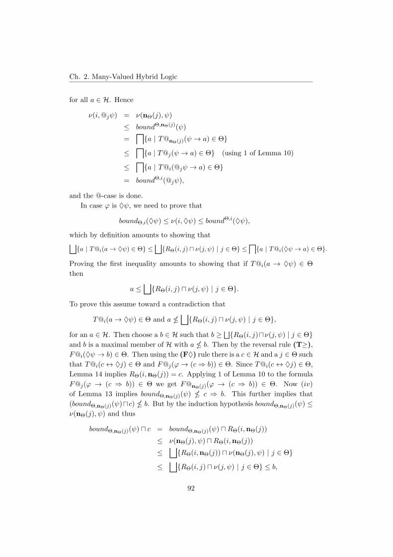
Ch. 2. Many-Valued Hybrid Logic

for all a ∈ H. Hence

ν(i,@jψ) = ν(nΘ(j), ψ)

≤ boundΘ,nΘ(j)(ψ)

=l{a | T@nΘ(j)(ψ → a) ∈ Θ}

≤l{a | T@j(ψ → a) ∈ Θ} (using 1 of Lemma 10)

≤l{a | T@i(@jψ → a) ∈ Θ}

= boundΘ,i(@jψ),

and the @-case is done.

In case ϕ is ♦ψ, we need to prove that

boundΘ,i(♦ψ) ≤ ν(i,♦ψ) ≤ boundΘ,i(♦ψ),

which by definition amounts to showing that⊔{a | T@i(a→ ♦ψ) ∈ Θ} ≤

⊔{RΘ(i, j) u ν(j, ψ) | j ∈ Θ} ≤

l{a | T@i(♦ψ → a) ∈ Θ}.

Proving the first inequality amounts to showing that if T@i(a → ♦ψ) ∈ Θ

then

a ≤⊔{RΘ(i, j) u ν(j, ψ) | j ∈ Θ}.

To prove this assume toward a contradiction that

T@i(a→ ♦ψ) ∈ Θ and a �⊔{RΘ(i, j) u ν(j, ψ) | j ∈ Θ},

for an a ∈ H. Then choose a b ∈ H such that b ≥⊔{RΘ(i, j)uν(j, ψ) | j ∈ Θ}

and b is a maximal member of H with a � b. Then by the reversal rule (T≥),

F@i(♦ψ → b) ∈ Θ. Then using the (F♦) rule there is a c ∈ H and a j ∈ Θ such

that T@i(c↔ ♦j) ∈ Θ and F@j(ϕ→ (c⇒ b)) ∈ Θ. Since T@i(c↔ ♦j) ∈ Θ,

Lemma 14 implies RΘ(i,nΘ(j)) = c. Applying 1 of Lemma 10 to the formula

F@j(ϕ → (c ⇒ b)) ∈ Θ we get F@nΘ(j)(ϕ → (c ⇒ b)) ∈ Θ. Now (iv)

of Lemma 13 implies boundΘ,nΘ(j)(ψ) � c ⇒ b. This further implies that

(boundΘ,nΘ(j)(ψ)uc) � b. But by the induction hypothesis boundΘ,nΘ(j)(ψ) ≤ν(nΘ(j), ψ) and thus

boundΘ,nΘ(j)(ψ) u c = boundΘ,nΘ(j)(ψ) uRΘ(i,nΘ(j))

≤ ν(nΘ(j), ψ) uRΘ(i,nΘ(j))

≤⊔{RΘ(i,nΘ(j)) u ν(nΘ(j), ψ) | j ∈ Θ}

≤⊔{RΘ(i, j) u ν(j, ψ) | j ∈ Θ} ≤ b,

92

2.5 Completeness of the basic calculus

which of course is a contradiction.

In order to prove that⊔{RΘ(i, j) u ν(j, ψ) | j ∈ Θ} ≤

l{a | T@i(♦ψ → a) ∈ Θ},

we must show that if T@i(♦ψ → a) ∈ Θ, then RΘ(i, j) u ν(j, ψ) ≤ a for all

j ∈ Θ. Thus assume that T@i(♦ψ → a) ∈ Θ and that RΘ(i, j) 6= ⊥ (or else

it’s trivial) for an arbitrary j ∈ Θ. Since RΘ(i, j) 6= ⊥, the definition of R

implies that j must be an urfather. Furthermore,

RΘ(i, j) =⊔{b | T@i(b→ ♦k) ∈ Θ,nΘ(k) = j}.

Let b and k be chosen arbitrarily such that T@i(b→ ♦k) ∈ Θ and nΘ(k) = j.

Then by the (T♦) rule, T@k(ψ → (b ⇒ a)) ∈ Θ. Using 1 of Lemma 10 we

get T@nΘ(k)(ψ → (b ⇒ a)) ∈ Θ, that is, T@j(ψ → (b ⇒ a)) ∈ Θ. Now, by

induction hypothesis, since j is an urfather,

ν(j, ψ) ≤ boundΘ,j(ψ) ≤ b⇒ a.

Since k and b were chosen arbitrarily with T@i(b→ ♦k) ∈ Θ and nΘ(k) = j,

we get

ν(j, ψ) ≤l{b⇒ a | T@i(b→ ♦k) ∈ Θ,nΘ(k) = j}.

We now get

RΘ(i, j) u ν(j, ψ) ≤⊔{b | T@i(b→ ♦k) ∈ Θ,nΘ(k) = j}

ul{b⇒ a | T@i(b→ ♦k) ∈ Θ,nΘ(k) = j}

≤⊔{b u (b⇒ a) | T@i(b→ ♦k) ∈ Θ,nΘ(k) = j}

≤⊔{a | T@i(b→ ♦k) ∈ Θ,nΘ(k) = j}

≤ a.

Because j ∈ Θ was arbitrary it follows that it holds for all j ∈ Θ and the proof

of this case is completed.In case ϕ is �ψ, we need to prove that⊔

{a | T@i(a→ �ψ) ∈ Θ} ≤l{RΘ(i, j)⇒ ν(j, ψ) | j ∈ Θ} ≤

l{a | T@i(�ψ → a) ∈ Θ}.

To prove the first inequality we need to prove that if j ∈ Θ, then

a ≤ RΘ(i, j)⇒ ν(j, ψ), (2.2)

93

Ch. 2. Many-Valued Hybrid Logic

for all a ∈ H with T@i(a→ �ψ) ∈ Θ. So let a ∈ H be given arbitrarily such

that T@i(a→ �ψ) ∈ Θ. Note that (2.2) is equivalent to

a uRΘ(i, j) ≤ ν(j, ψ).

By definition of RΘ we have

RΘ(i, j) =⊔{b | T@i(b→ ♦k) ∈ Θ,nΘ(k) = j}.

Let b and k be chosen arbitrarily such that T@i(b→ ♦k) ∈ Θ and nΘ(k) = j.

Then by the (T�)-rule it follows that T@k((a u b) → ψ) ∈ Θ. By 1 of

Lemma 10 this implies T@j((a u b) → ψ) ∈ Θ. Thus we get boundΘ,j(ψ) ≥(a u b). Since b and k were chosen arbitrarily with the properties T@i(b →♦k) ∈ Θ and nΘ(k) = j we then get

boundΘ,j(ψ) ≥⊔{a u b | T@i(b→ ♦k) ∈ Θ,nΘ(k) = j}.

Using this inequality and the induction hypothesis we now get

a uRΘ(i, j) = a u⊔{b | T@i(b→ ♦k) ∈ Θ,nΘ(k) = j}

=⊔{a u b | T@i(b→ ♦k) ∈ Θ,nΘ(k) = j}

≤ boundΘ,j(ψ) ≤ ν(j, ψ).

Since a was arbitrary this holds for all a ∈ H and the inequality have been

proven.

To show the other inequality we need to show that

if T@i(�ψ → a) ∈ Θ thenl{RΘ(i, j)⇒ ν(j, ψ) | j ∈ Θ} ≤ a.

If a = > then this is trivial. Thus assume towards a contradiction that there

is an a 6= > with T@i(�ψ → a) ∈ Θ andd{RΘ(i, j) ⇒ ν(j, ψ) | j ∈ Θ} � a.

Now let b ≤d{RΘ(i, j) ⇒ ν(j, ψ) | j ∈ Θ} be a minimal member of H such

that b � a. Then by the reversal rule (T≤), F@i(b→ �ψ) ∈ Θ. Hence by the

(F�)-rule there is a nominal k ∈ Θ and a c ∈ H such that T@i(c↔ ♦k) ∈ Θ

and F@k((b u c) → ψ) ∈ Θ. From the first it follows that RΘ(i,nΘ(k)) = c,

using Lemma 14. From the second it follows that F@nΘ(k)((b u c)→ ψ) ∈ Θ,

using 1 of Lemma 10, and thus, by (iii) of Lemma 13, buc � boundΘ,nΘ(k)(ψ).

But then from the induction hypothesis it follows that

b u c � ν(nΘ(k), ψ) ≤ boundΘ,nΘ(k)(ψ).

94

2.5 Completeness of the basic calculus

Hence

b � c⇒ ν(nΘ(k), ψ) = RΘ(i,nΘ(k))⇒ ν(nΘ(k), ψ).

But by the assumption on b we also have that

b ≤l{RΘ(i, j)⇒ ν(j, ψ) | j ∈ Θ} ≤ RΘ(i,nΘ(k))⇒ ν(nΘ(k), ψ),

and a contradiction have been reached. This concludes the � case and thus

the entire proof of the theorem.

Now completeness can easily be proven, in the following sense.

Theorem 16. If there is no tableau proof of the formula ϕ, then there is a

model M = 〈W,R,n, ν〉 and a w ∈W such that ν(w,ϕ) 6= >.

Proof. Assume that there is no tableau proof of the formula ϕ. Then there is

an saturated tableau with a open branch Θ starting with the formula F@i(> →ϕ) for a nominal i not in ϕ. By item 1 of Lemma 10 it follows that also

F@nΘ(i)(> → ϕ) ∈ Θ.

The model MΘ = 〈WΘ, RΘ,nΘ, νΘ〉 can now be constructed such that

νΘ satisfies the assumption of Theorem 15. Since F@nΘ(i)(> → ϕ) ∈ Θ it

follows by Lemma 13 that > � boundΘ,nΘ(i)(ϕ). But by Theorem 15, since ϕ

is a subformula of the root formula and nΘ(i) is an urfather, we know that

νΘ(nΘ(i), ϕ) ≤ boundΘ,nΘ(i)(ϕ) and it thus follows that > � νΘ(nΘ(i), ϕ) and

the proof is completed.

Acknowledgment

Thanks to the anonymous reviewers of AiML 2008 for useful comments and

corrections. The second and third authors are partially funded by the Danish

Natural Science Research Council (the HyLoMOL project).

95

Ch. 2. Many-Valued Hybrid Logic

96

Chapter 3

Alternative semantics for a

many-valued hybrid logic

Unpublished manuscript.

Abstract: In the paper [83] (Chapter 2) a many-valued hybrid

logic was introduced as an extension of a many-valued modal logic

of Fitting [59, 60, 61]. It was argued that the choice of semantics

for the hybrid machinery was the most natural generalization of the

standard semantics for hybrid logic. In this paper, alternative ways

of defining the semantics of the hybrid machinery are discussed and

compared to semantics of [83].

Keywords: Hybrid logic, many-valued modal logic, nominals, the

satisfaction operator, many-valued hybrid logic semantics.

This paper is a supplement to the paper [83] on many-valued hybrid logic.

In [83] particular semantics are chosen for the hybrid part of the language.

Nevertheless, other alternative definitions of the semantics are possible and in

the present paper we will consider such alternatives. We will look at five other

possible logics, even though many more are possible. However, the discussion

of these five logics will show that the semantics chosen in [83] is presumably

the most natural hybrid extension of the underlying many-valued modal logic.

We will use the same syntax for the language as in [83], and we will denote

the logic of that paper by MVHL. As in [83] we will only consider sets of

truth-values that are finite Heyting algebras. Compared to MVHL, we will

focus on the possibility of changing only two things; the way nominals are

interpreted in a model, and how the semantics of the satisfaction operator @i

is defined. An exception will be the logic MVHL3 where we will also place an

97

Ch. 3. Alternative semantics for a many-valued hybrid logic

extra requirement on the Heyting algebras. Note, in particular, that we will

change neither the semantics of the modalities � and ♦, nor the semantics of

the global modalities A and E.

The new logics introduced in this paper will be compared to the logic of

[83] on four aspects. One key feature of hybrid logic is that it allows for

equational reasoning about worlds in the language. This is due to the fact

that the formula @ij expresses equality between the two worlds denoted by i

and j. In the many-valued setting of [83], this feature reveals itself as the fact

that

ν(w,@ij) = > iff n(i) = n(j).

Another key feature of hybrid logic is its ability to express accessibility

between worlds, in the sense that @i♦j is true if and only if the world denoted

by j is accessible by the world denoted by i. In the many-valued setting of

[83] this is again the case since the truth value of the accessibility between the

world denoted by i and the world denoted by j, R(n(i),n(j)), is equal to the

truth value of the formula @i♦j.

The third property of standard hybrid logic is the fact that the satisfaction

operator can be defined by nominals and the global modality. This is due to

the fact that the truth values of the formulas @iϕ, E(i ∧ ϕ), and A(i → ϕ)

are equal. This is also the case for the logic of [83]. Note that the question

of whether @iϕ can be defined as E(i ∧ ϕ) and A(i→ ϕ), actually consists of

three questions, namely the question of whether @iϕ is equivalent to E(i∧ϕ),

whether @iϕ is equivalent to A(i → ϕ), and, finally, whether E(i ∧ ϕ) and

A(i → ϕ) are equivalent. A consequence of this paper is the realization that

the answers to these three questions are independent.1

Finally, the fourth property of the logic of [83] that makes it a natural

extension of standard hybrid logic is the fact that if the truth value set is the

simple Heyting algebra {>,⊥}, then the logic collapses to standard hybrid

logic.

In the following five sections we will present five different logics that are all

variations of the original MVHL. We will end each section with a summary

on the differences and similarities between the given logic and MVHL, based

1Note that we will only compare logics on whether the satisfaction operator is definable

by E(i ∧ ϕ) or A(i → ϕ), not whether the satisfaction operator is definable from nominals

and global modalities in general. The same issue arises in the question of defining equality

or accessibility between worlds. See Section 3.7 for further discussions.

98

3.1 MVHL1

on the four mentioned properties. Our findings are simplified in Figure 3.1.

In the end, we will give a short conclusion and direction for further research.

3.1 MVHL1

In the semantics of MVHL every nominal was assigned > in one world and ⊥in the rest. We keep the requirement that nominals are assigned > in exactly

one world, but do not put any requirement on what they are assigned in other

worlds (as long as it is not >). This leads to a new definition of a model;

however, the only thing we change is the nominal assignment n.

Definition 17 (Alternative notion of a model). A model M is a tuple M =

〈W,R, ν,n〉, where 〈W,R, ν〉 is the same as for standard MVHL, but now

n : W × NOM → H and for all i ∈ NOM there is a unique w ∈ W such that

ν(w, i) = >. For all i ∈ NOM, the unique w such that ν(w, i) = > will be

denoted by i and referred to as the denotation of i.

The valuation ν can now be extended to all MVHL-formulas almost as

before. The semantic of the nominal i at the world w is given by

ν(w, i) = n(w, i).

Furthermore, the semantic of @iϕ needs to be changed as well and we choose

to define it in the following way:

ν(w,@iϕ) = ν (i, ϕ), (3.1)

where i is the denotation of i as defined in Definition 17. By this definition

the truth value of the formula @iϕ is precisely the truth value of ϕ at the

world denoted by the nominal i. Call the logic obtained by this semantics for

MVHL1.

How does the new logic MVHL1 looks compared to MVHL? First, note

that ν(w, i) still gets the value > in exactly one world, and therefore nominals

still denote single worlds in a sense. As a consequence, the logic can still

express equality of worlds because:

ν(w,@ij) = > iff i = j,

for all i, j ∈ NOM, all MVHL1-models M = 〈W,R, ν,n〉 and all w ∈ W .

That this is true is not hard to see from the definition of the semantics.

99

Ch. 3. Alternative semantics for a many-valued hybrid logic

However, the two logics do differ considerably. The accessibility between

worlds are no longer expressible in the same way. Consider the following

example:

Example 18. Let H = {⊥, a, b,>} be such that neither a ≤ b nor b ≤ a, and

thus a t b = >.2 Let the model M = 〈W,R, ν,n〉 satisfy the following:

W = {w0, w1};

R(w0, w0) = b, R(w0, w1) = a;

n(w0, i) = >, n(w1, i) = ⊥;

n(w0, j) = b, n(w1, j) = >,

for distinct nominals i and j. Then, we have for all w ∈W that

ν(w,@i♦j) = ν (i,♦j)

=⊔{R(i, v) u ν(v, j) | v ∈W}

=(R(i, w0) u n(w0, j)

)t(R(i, w1) u n(w1, j)

)= b t a= >6= a = R(i, j).

Note, however, that we do have that R(i, j) ≤ ν(w,@i♦j) always holds.3

Furthermore, the semantic of @iϕ can no longer be defined in terms of the

global modalities E or A. This can be seen by the following example:

Example 19. Let H = {⊥, a,>} be a Heyting algebra and define the model

M = 〈W,R, ν,n〉, such that:

W = {w0, w1};

n(w0, i) = >, n(w1, i) = a;

ν(w0, p) = ⊥, ν(w1, p) = a,

2Note that H actually is a Heyting algebra, which is easy to see.3In

⊔{R(i, v) u ν(v, j) | v ∈W}, if v = j then R(i, v) u ν(v, j) = R(i, j) and thus

R(i, j) ≤⊔{R(i, v) u ν(v, j) | v ∈W} = ν(w,@i♦j).

100

3.1 MVHL1

for an i ∈ NOM and p ∈ PROP. In this model ν(w,@ip) = ν (i, p) = ν(w0, p) =

⊥. Nevertheless,

ν(w,E(i ∧ p)) =⊔{ν(v, i) u ν(v, p) | v ∈W}

=(n(w0, i) u ν(w0, p)

)t(n(w1, i) u ν(w1, p)

)= ⊥ t a= a,

and since ⊥ 6= a, @ip and E(i∧ p) are not equivalent. Actually, in this model

ν(w,A(i→ p)) =l{ν(v, i)⇒ ν(v, p) | v ∈W}

= (n(w0, i)⇒ ν(w0, p)) u (n(w1, i)⇒ ν(w1, p))

= ⊥ u>= ⊥.

However, if the values of ν(w0, p) and ν(w1, p) are interchanged then ν(w,A(i→p)) = ⊥ still holds, but now ν(w,@ip) = a will be the case.

The above example also shows that E(i ∧ ϕ) and A(i→ ϕ) are not equiv-

alent in general in MVHL1, as is the case for MVHL (in MVHL they are

both equivalent to @iϕ). But the formulas E(i ∧ ϕ) and A(i → ϕ) are still

related to the formula @iϕ since we have the following inequality in MVHL1:

ν(w,A(i→ ϕ) ≤ ν(w,@iϕ) ≤ ν(w,E(i ∧ ϕ)),

for all w ∈W . This follows from the following calculations:

ν(w,A(i→ ϕ)) =l{ν(v, i)⇒ ν(v, ϕ) | v ∈W}

≤ ν (i, i)⇒ ν (i, ϕ)

= ν (i, ϕ) (= ν(w,@iϕ)) (3.2)

= ν (i, i) u ν (i, ϕ)

≤⊔{ν(v, i) u ν(v, ϕ) | v ∈W}

= ν(w,E(i ∧ ϕ)).

Observe, that ifH = {>,⊥} (i.e. we are in the classical two-valued setting),

then the logic MVHL1 reduces to the logic MVHL. Thus, MVHL1 also

extends classical two-valued hybrid logic.

Summary 20 (MVHL1 vs. MVHL). We summarize the semantic differ-

ences and similarities between MVHL1 and MVHL:

101

Ch. 3. Alternative semantics for a many-valued hybrid logic

• As was the case for MVHL, equality between worlds can be expressed in

MVHL1 since the following holds in MVHL1:

ν(w,@ij) = > iff i = j

• However, accessibility between worlds is not expressible in MVHL1, in

the sense that ν(w,@i♦j) = R(i, j) does not hold in general. We do have

R(i, j) ≤ ν(w,@i♦j) though.

• Furthermore, @iϕ is not definable from the global modalities in the usual

way. Still, we have the following

ν(w,A(i→ ϕ) ≤ ν(w,@iϕ) ≤ ν(w,E(i ∧ ϕ)).

None of the inequalities can be replaced by equality in general. As a

byproduct, A(i→ ϕ) and E(i ∧ ϕ) are not equivalent in MVHL1.

• Finally, as for MVHL, MVHL1 collapses to standard two-valued hybrid

logic in the case T = {>,⊥}.

3.2 MVHL2

In MVHL1 the definability of @iϕ in terms of the global modalities fails.

However, if we want to take this problem seriously, we could just change the

semantic of @iϕ such that it matches that of E(i ∧ ϕ).4 This we will now

do. Call the logic obtained by replacing the semantic definition (3.1) by (3.3)

MVHL2, where

ν(w,@iϕ) =⊔{ν(v, i) u ν(v, ϕ) | v ∈W}. (3.3)

Then, it follows directly from the definition that in MVHL2, ν(w,@iϕ) =

ν(w,E(i ∧ ϕ)).5 Now, what about the other properties of this logic? This

time it is the characterization of equality of worlds by @ij that fails. Note,

that the notion of a model for MVHL2 is the same as for MVHL1, i.e.

Definition 17. Now, consider the following example:

Example 21. Let H be as in Example 18 and let the model M = 〈W,R, ν,n〉satisfy:

4Alternatively, we could have changed the semantic of @iϕ such that it matches that of

A(i→ ϕ). This we will do in Section 3.4.5As before, we still have that ν(w,A(i → ϕ)) ≤ ν(w,@iϕ) and that equality does not

hold in general.

102

3.2 MVHL2

W = {w0, w1, w2, w3};

n(w0, i) = a, n(w1, i) = b, n(w2, i) = ⊥, n(w3, i) = >;

n(w0, j) = a, n(w1, j) = b, n(w2, j) = >, n(w3, j) = ⊥,

for distinct nominals i and j. In this model we have for all w ∈W that

ν(w,@ij) =⊔{ν(v, i) u ν(v, j) | v ∈W}

=(n(w0, i) u n(w0, j)

)t(n(w1, i) u n(w1, j)

)t(n(w2, i) u n(w2, j)

)t(n(w3, i) u n(w3, j)

)= a t b t ⊥ t ⊥ = >,

however, i = w3 6= w2 = j.

ν(w,@ij) = > does not guarantee that i and j denote the same world,

nevertheless, the other implication, “if i = j then ν(w,@ij) = >”, does hold.

Now, take the model of Example 18 again. With the MVHL2 semantics

we have that

ν(w,@i♦j) =⊔{ν(v, i) u ν(v,♦j) | v ∈W}

=(n(w0, i) u ν(w0,♦j)

)t(n(w1, i) u ν(w1,♦j)

)=

(> u

⊔{R(w0, u) u ν(u, j) | u ∈W}

)t(⊥ u

⊔{R(w1, u) u ν(u, j) | u ∈W}

)=

((R(w0, w0) u n(w0, j)

)t(R(w0, w1) u n(w1, j)

))t ⊥

= b t a= >,

however, R(i, j) = a 6= >. This shows that the formula @i♦j does not express

accessibility between the worlds denoted by i and j in MVHL2. Nonetheless,

we still have the inequality R(i, j) ≤ ν(w,@i♦j).6

Finally, note that if H = {>,⊥}, then

ν(w,@iϕ) =⊔{ν(v, i) u ν(v, ϕ) | v ∈W} = ν (i, i) u ν (i, ϕ) = ν (i, ϕ),

Thus, in the case H = {>,⊥}, MVHL2 collapses to MVHL1 and thus also

to standard two-valued hybrid logic.

6This is because: ν(w,@i♦j) =⊔{ν(v, i)u ν(v,♦j) | v ∈W} =

⊔{n(v, i)u

(⊔{R(v, u)u

n(u, j) | u ∈ W})| v ∈ W} =

⊔{⊔{n(v, i) u R(v, u) u n(u, j) | u ∈ W} | v ∈ W} ≥

n(i, i) uR(i, j) u n(j, j) = R(i, j).

103

Ch. 3. Alternative semantics for a many-valued hybrid logic

Summary 22 (MVHL2 vs. MVHL). We summarize the semantic differ-

ences and similarities between MVHL2 and MVHL:

• Contrary to MVHL, equality between worlds cannot be expressed by the

formula @ij in MVHL2.

• Accessibility between worlds is not expressible in MVHL2 either, since

ν(w,@i♦j) = R(i, j) does not hold in general, though R(i, j) ≤ ν(w,@i♦j)still holds.

• We have that @iϕ is equivalent to E(i∧ϕ) by definition, but the inequality

ν(w,A(i→ ϕ)) ≤ ν(w,E(i ∧ ϕ))

cannot be replaced by equality in general for MVHL2 either.

• Finally, as for MVHL, MVHL2 collapses to standard two-valued hybrid

logic in the case T = {>,⊥}.

3.3 MVHL3

It turns out that the lack of power in MVHL2 to express equality of worlds

using nominals can be fixed by placing a requirement on the Heyting algebra

H. First a definition (adopted from [48], page 53):

Definition 23. Let H be a finite Heyting algebra. An element a ∈ H is called

join-irreducible if a 6= ⊥ and for all x, y ∈ H, a = x t y implies that a = x or

a = y.

The requirement that will be placed on the Heyting algebra H is that

> is join-irreducible. Note that, if H = {>,⊥}, then > is join-irreducible.

Moreover, if H is a linear ordered finite Heyting algebra, then > is also join-

irreducible. Thus, in the Heyting algebra of Example 19 > is join-irreducible

whereas > is not join-irreducible in Heyting algebra of Example 18. We now

have the following result:

Theorem 24. For all MVHL2 models M = 〈W,R, ν,n〉 build on a Heyting

algebra where > is join-irreducible, the following holds:

ν(w,@ij) = > iff i = j, (3.4)

for all i, j ∈ NOM and all w ∈W .

104

3.3 MVHL3

Proof. Assume that M = 〈W,R, ν,n〉 is a model built on a Heyting algebra

where > is join-irreducible. As mentioned before the “if” part is easy and

always holds. So assume now that ν(w,@ij) = > for a w ∈ W and two

nominals i and j. Then we need to prove that i = j. However, since

> = ν(w,@ij) =⊔{ν(v, i) u ν(v, j) | v ∈W},

and > is join-irreducible, there must be a v ∈W such that ν(v, i)uν(v, j) = >.

This again is only possible if both ν(v, i) = > and ν(v, j) = >, and thus

i = j.

There is a sense in which the other “implication” of Theorem 24 is also true:

We can characterize the finite Heyting algebras where > is join-irreducible by

the property (3.4). Thus we have a characterization not of a class of frames

but a class of Heyting algebras acting as premissible sets of truth values:

Theorem 25. For a finite Heyting algebra H, > is join-irreducible if and only

if the following property holds:

(∗) For all MVHL2-models M = 〈W,R, ν,n〉, for all w ∈ W ,

and for all nominals i and j

ν(w,@ij) = > iff i = j.

Proof. Then one direction, namely the fact that “if > is join-irreducible in Hthen (∗) holds” is a direct consequence of Theorem 24. For the other direction

assume that H is a finite Heyting algebra satisfying (∗). Assume towards a

contradiction that > is not join-irreducible in H. Then there must be two

distinct elements a and b of H strictly below > such that neither a ≤ b or

b ≤ a, but a t b = >.

Now define a MVHL2 model M = 〈W,R, ν,n〉 such that

W = {w0, w1};

n(w0, i) = >, n(w1, i) = a;

n(w0, j) = b, n(w1, j) = >,

for two distinct nominals i and j. Then

ν(w,@ij) =⊔{ν(v, i) u ν(v, j) | v ∈W}

=(n(w0, i) u n(w0, j)

)t(n(w1, i) u n(w1, j)

)= (> u b) t (a u >)

= b t a = >,

105

Ch. 3. Alternative semantics for a many-valued hybrid logic

and since H satisfies (∗) it follows that i = j. However, this is a contradiction

since in M, i = w0 6= w1 = j. Thus, > must be join-irreducible in H and the

proof is completed.

The logic obtained from MVHL2 by only allowing finite Heyting algebras

where > is join-irreducible will be denoted by MVHL3. Again, the notion of

a MVHL3-model is the same as in Definition 17.

We now look at the formula @i♦j and the possibility of defining accessi-

bility between worlds in MVHL3. Assume that > is join-irreducible in the

Heyting algebra H. Because,

ν(w,@i♦j) =⊔{ν(v, i) u ν(v,♦j) | v ∈W},

ν(w,@i♦j) can only be > if there is a v ∈W such that ν(v, i)u ν(v,♦j) = >.

Thus, we have for MVHL3 that

ν(w,@i♦j) = > iff R(i, j) = >.

This is contrary to MVHL2 where we showed that in Example 18, R(i, j) = a,

but ν(w,@i♦j) = >. Furthermore, as for MVHL1 and MVHL2 we have

that the inequality R(i, j) ≤ ν(w,@i♦j) holds in general. Nevertheless, if

R(i, j) < >, then R(i, j) < ν(w,@i♦j) can occur in MVHL3, as the following

example shows:

Example 26. Let H = {>, a, b,⊥} be a Heyting algebra such that ⊥ < b <

a < >. Note that, since H is a linear order, > is join-irreducible. Let the

model M = 〈W,R, ν,n〉 satisfy:

W = {w0, w1};

R(w0, w0) = a, R(w0, w1) = b;

n(w0, i) = >, n(w1, i) = a;

n(w0, j) = a, n(w1, j) = >,

for distinct nominals i and j. In this model we have

ν(w,@i♦j) =⊔{ν(v, i) u ν(v,♦j) | v ∈W}

=⊔{n(v, i) u

(⊔{R(v, u) u n(u, j) | u ∈W}

)| v ∈W}

=⊔{⊔{n(v, i) uR(v, u) u n(u, j) | u ∈W} | v ∈W}

≥ n(w0, i) uR(w0, w0) u n(w0, j)

= > u a u a = a,

106

3.4 MVHL4

and thus, R(i, j) = b < a ≤ ν(w,@i♦j).

At last, note that since nothing has been changed in the semantics of @i

and E relative to MVHL2, the formulas @iϕ and E(i∧ϕ) are still equivalent.

The equality ν(w,A(i → ϕ)) ≤ ν(w,E(i ∧ ϕ)) also holds for MVHL3 and

Example 19 can be used again to show that this inequality can be strict.

Summary 27 (MVHL3 vs. MVHL). We summarize the semantic differ-

ences and similarities between MVHL3 and MVHL:

• As in MVHL (contrary to MVHL2), equality between worlds can be

expressed by the formula @ij in MVHL3.

• Accessibility between worlds is not generally expressible in MVHL3 ei-

ther, since ν(w,@i♦j) = R(i, j) does not hold in general. However, in

MVHL3 we have that R(i, j) ≤ ν(w,@i♦j) and furthermore that

ν(w,@i♦j) = > iff R(i, j) = >.

• We have that @iϕ is equivalent to E(i∧ϕ) by definition, but the inequality

ν(w,A(i→ ϕ)) ≤ ν(w,E(i ∧ ϕ))

cannot be replaced by equality in general for MVHL3 either.

• Finally, as for MVHL, MVHL3 collapses to standard two-valued hybrid

logic in the case T = {>,⊥}.

3.4 MVHL4

In MVHL2 we chose to make the semantic of @iϕ equal that of E(i∧ϕ). We

now make the semantic of @iϕ equal to that of A(i→ ϕ). Thus, let the logic

MVHL4 be the logic obtained from MVHL2 by replacing the semantic of

@iϕ (given in (3.3)), with the following definition:

ν(w,@iϕ) =l{ν(v, i)⇒ ν(v, ϕ) | v ∈W}. (3.5)

At first glance, one may except that a logic similar to MVHL2 will be

the result. However, there are some interesting differences. In fact, equality

between worlds becomes expressible now. Let a model M = 〈W,R, ν,n〉 be

given. If ν(w,@ij) = > then by the definition (3.5) it follows that:

ν(v, i)⇒ ν(v, j) = > , for all v ∈W.

107

Ch. 3. Alternative semantics for a many-valued hybrid logic

This further implies that:

ν(v, i) ≤ ν(v, j) , for all v ∈W, (3.6)

but if i 6= j, then there is an a ∈ H such that ν (i, j) = a < > = ν (i, i).

Hence, if ν(w,@ij) = > it follows that i = j. Yet, an important thing to

note is that i = j does not imply that ν(w,@ij) = >. What is required for

ν(w,@ij) = > to be true, is the stronger requirement that (3.6) is satisfied.

That @ij expresses an inequality instead of equality is also evident from the

fact that @ij and @ji are not equivalent formulas in MVHL4. All of this is

made clear in the following example:

Example 28. Let H be as in Example 18. And let the modelM = 〈W,R, ν,n〉satisfy:

W = {w0, w1};

n(w0, i) = >, n(w1, i) = a, n(w0, j) = >, n(w1, j) = b,

for distinct nominals i and j. Then i = j, although

ν(w,@ij) = (ν(w0, i)⇒ ν(w0, j)) u (ν(w1, i)⇒ ν(w1, j))

= (> ⇒ >) u (a⇒ b)

= > u b = b

ν(w,@ji) = (ν(w0, j)⇒ ν(w0, i)) u (ν(w1, j)⇒ ν(w1, i))

= (> ⇒ >) u (b⇒ a)

= > u a = a

We now inspect the formula @i♦j. With the Heyting algebra and model

of Example 18 we have that:

ν(w,@i♦j) =l{ν(v, i)⇒ ν(v,♦j) | v ∈W}

= (ν(w0, i)⇒ ν(w0,♦j)) u (ν(w1, i)⇒ ν(w1,♦j))

= (> ⇒⊔{R(w0, u) u ν(u, j) | u ∈W})

u (⊥ ⇒⊔{R(w1, u) u ν(u, j) | u ∈W})

=⊔{R(w0, u) u ν(u, j) | u ∈W} u >

= (R(w0, w0) u ν(w0, j)) t (R(w0, w1) u ν(w1, j))

= (b u b) t (a u >)

= b t a = >.

108

3.5 MVHL5

However, R(i, j) = a. Hence, as for MVHL2, @i♦j does not express accessi-

bility between the worlds denoted by i and j.

Since nothing has been changed for the global modalities, when we moved

from MVHL2 to MVHL4, the inequality

ν(w,A(i→ ϕ)) ≤ ν(w,E(i ∧ ϕ))

still holds and it cannot be replaced by equality in general. Furthermore, it is

obvious that @iϕ is equivalent to A(i→ ϕ) by definition.

At last, it is not hard to see that also MVHL4 collapses to the stan-

dard two-valued hybrid logic in the case when H = {>,⊥}. Once again we

summarize the logic:

Summary 29 (MVHL4 vs. MVHL). We summarize the semantic differ-

ences and similarities between MVHL4 and MVHL:

• In MVHL4, equality between worlds can be expressed in some sense

since ν(w,@ij) = > implies that i = j, but i = j does not implies

that ν(w,@ij) = > in general. In addition, @ij and @ji are not even

equivalent.

• Accessibility between worlds is not generally expressible in MVHL4,

since ν(w,@i♦j) = R(i, j) is not the case in general.

• @iϕ is equivalent to A(i→ ϕ) by definition, but the inequality

ν(w,A(i→ ϕ)) ≤ ν(w,E(i ∧ ϕ))

can still not be replaced by equality in general for MVHL4.

• Finally, as for MVHL, MVHL4 collapses to standard two-valued hybrid

logic in the case T = {>,⊥}.

3.5 MVHL5

The different logics discussed so far have all been based on the same notion of

a model, the one given in Definition 17. We will now change the notion of a

model. Instead of letting nominals point out single worlds, we let them point

out sets of worlds whose truth-values of the nominal “sum up” to >. This is

spelled out in details in the following definition:

109

Ch. 3. Alternative semantics for a many-valued hybrid logic

Definition 30 (Alternative2 definition of models). A modelM = 〈W,R, ν,n〉is as in Definition 17, but the requirement on n has been changed to:

For all nominals i ∈ NOM, there is a unique finite set Wi ⊆ W

such that

i)⊔w∈Wi

n(w, i) = >.

ii) There is no proper subset of Wi for which i) holds.

iii) For all w /∈Wi, n(w, i) = ⊥.

Note, that models for the original logic MVHL can also be viewed as

models according to this definition. Now, we can interpret the language of

MVHL over this new class of models. To see which kind of logic that results

from this, the problem of defining the semantic for @iϕ needs to be attended.

We choose the following semantic for @iϕ:

ν(w,@iϕ) =⊔{ν(v, i) u ν(v, ϕ) | v ∈Wi}, (3.7)

where Wi is the finite set of Definition 30. We will define MVHL5 to be

the logic obtained by interpreting the MVHL language only over alternative2

models where the truth definition of @iϕ is given by (3.7). Note, that due to

the requirement iii) of Definition 30, the definition (3.7) is equivalent to the

one of MVHL2 and MVHL3 given in (3.3). Thus, it further follows that in

MVHL5, @iϕ is equivalent to E(i ∧ ϕ). Now, however, the “trick” with i we

used in (3.2), to prove the inequality ν(w,A(i→ ϕ)) ≤ ν(w,E(i∧ϕ)), cannot

be used in MVHL5. In fact, it turns out that there is no general inequality

or equality between the formulas E(i ∧ ϕ) and A(i → ϕ). This is shown by

the following example:

Example 31. Let H = {⊥, a, b,>} be a Heyting algebra such that neither

a ≤ b nor b ≤ a, and thus a t b = >, a u b = ⊥. Now, let the model

M = 〈W,R, ν,n〉 satisfy the following:

W = {w0, w1, w2};

n(w0, i) = a, n(w1, i) = b, n(w2, i) = ⊥;

n(w0, j) = ⊥, n(w1, j) = a, n(w2, j) = b;,

for distinct nominals i and j. Given a propositional variable p, we have that

ν(w,E(i ∧ p)) =⊔{ν(v, i) u ν(v, p) | v ∈W} = (a u ν(w0, p)) t (b u ν(w1, p));

ν(w,A(i→ p)) =l{ν(v, i)⇒ ν(v, p) | v ∈W} = (a⇒ ν(w1, p)) u (b⇒ ν(w2, p)).

110

3.5 MVHL5

If we let the semantic of p be given by ν(w0, p) = >, ν(w1, p) = ⊥, ν(w2, p) =

⊥, then we have:

ν(w,E(i ∧ p)) = (a u >) t (b u ⊥) = a t ⊥ = a;

ν(w,A(i→ p)) = (a⇒ ⊥) u (b⇒ ⊥) = b u a = ⊥.

On the other hand, if we let the semantic of p be given by ν(w0, p) = >, ν(w1, p) =

a, ν(w2, p) = >, we have:

ν(w,E(i ∧ p)) = (a u >) t (b u a) = a t ⊥ = a;

ν(w,A(i→ p)) = (a⇒ a) u (b⇒ >) = > u> = >.

Since nominals no longer denote single worlds, we cannot talk about equal-

ity of worlds at all. However, we can speak about equality between sets of

worlds. Let i and j be distinct nominals and let Wi and Wj be as in Defini-

tion 30. Then,

ν(w,@ij) =⊔{ν(v, i) u ν(v, j) | v ∈Wi}

=⊔{ν(v, i) u ν(v, j) | v ∈ (Wi ∩Wj)},

because of requirement iii) of Definition 30. But then because of requirement

i) and ii) it follows that

ν(w,@ij) = > iff Wi = Wj .

Hence, in MVHL5 the formula @ij expresses the equality between the sets

Wi and Wj .

Assume now that H = {>,⊥}. Then, for every nominal i ∈ NOM we have

that Wi must be a singleton in every model, otherwise the model would not

satisfy Definition 30. The definition of the semantic of @iϕ also collapses to

the usual one for hybrid logic and thus, once again we are dealing with a logic

that collapses to the standard two-valued hybrid logic when T = {>,⊥}.Finally, we now turn to the formula @i♦j. At first glance it seems like the

formula @i♦j expresses a form of “weighted sum” of accessibility of the Wj

worlds from the Wi worlds since

ν(w,@i♦j) =⊔{ν(v, i) u ν(v,♦j) | v ∈Wi}

=⊔{ν(v, i) u

⊔{R(v, t) u ν(t, j) |t ∈W} | v ∈Wi}

=⊔{⊔{ν(v, i) uR(v, t) u ν(t, j) |t ∈W} | v ∈Wi}

=⊔{ν(v, i) uR(v, t) u ν(t, j) |(v, t) ∈Wi ×Wj}.

111

Ch. 3. Alternative semantics for a many-valued hybrid logic

However, which notion of accessibility between sets of worlds, based on an

underlying accessibility relation between worlds, is the right notion is not

obvious. Thus, at the current state, we do not gain much from evaluating

MVHL5 on the basis of the formulas @i♦j.

Summary 32 (MVHL5 vs. MVHL). We summarize the semantic differ-

ences and similarities between MVHL5 and MVHL:

• In MVHL5 we cannot express equality between worlds (contrary to MVHL),

but we can express equality between sets of worlds, which seems to be the

only reasonable thing given the interpretation of nominals in a model.

• Since we cannot talk about worlds, we cannot express accessibility between

worlds. However, we can express some sort of accessibility between sets

of worlds. What this accessibility amounts to is still unclear.

• In MVHL5 the formula @iϕ is equivalent to E(i ∧ ϕ) as in MVHL.

Nevertheless, there are in general no equality or even inequality between

the formulas ν(w,A(i→ ϕ)) and ν(w,E(i ∧ ϕ)).

• Finally, as for all the other versions of MVHL, MVHL5 collapses to

standard two-valued hybrid logic in the case T = {>,⊥}.

3.6 Still more logics!

In MVHL5 we chose to let the semantic of @iϕ be equal to that of E(i ∧ ϕ).

Yet another logic could be obtained by letting the semantic of @iϕ be equal

to that of A(i→ ϕ). This we will not do in details here though. It would not

change the relationship between the semantics of E(i ∧ ϕ) and A(i→ ϕ) and

it will still be an extension of standard two valued hybrid logic. The formula

@i♦j will receive a new semantic, but we still do not have any concept to

compare it against. Finally, what the formula @ij expresses is still a little

unclear.

There are still more possible variations of MVHL5. One obvious way to

go would be to drop requirement iii) of Definition 30. However, we have seen

enough logics, and we will leave this for further research.

3.7 Concluding remarks and further research

In this paper, we presented five alternative many-valued hybrid logics, which

were all obtained by making small changes to the many-valued hybrid logic of

112

3.7 Concluding remarks and further research

MVHL1 MVHL2 MVHL3 MVHL4 MVHL5

ν(w,@ij) = > iff i = j yes no yes no no /

holds in general (⇒ holds) yes

ν(w,@i♦j) = R(i, j) no no no no no

holds in general (≥ holds) (≥ holds) (≥ holds) (undef.)

ν(w,A(i→ϕ)) = ν(w,@iϕ) no no no yes no

holds in general (≤ holds) (≤ holds) (≤ holds) (by def.)

ν(w,@iϕ) = ν(w,E(i ∧ ϕ)) no yes yes no yes

holds in general (≤ holds) (by def.) (by def.) (≤ holds) (by def.)

Collapses to MVHL yes yes yes yes yes

when H = {>,⊥}

Figure 3.1: Comparison between the logics MVHL1-MVHL5

[83]. We compared all the logics to the one in [83] on four matters; how well

they were capable of expressing equality between worlds, how well they were

capable of expressing the accessibility between worlds, how the semantic of the

formula @iϕ related to the semantics of the formulas E(i ∧ ϕ) and A(i→ ϕ),

and whether they could be viewed as extensions of the standard two-valued

hybrid logic. Our findings are summarized in Figure 3.1.

The five new logics were all extensions of standard two-valued hybrid logic,

but all of them differed from the logic of [83] with respect to at least one of the

other matters. Thus, if one argues for a many-valued extension of standard

two-valued hybrid logic, in which equality between worlds and accessibility

between worlds are expressible and where the formulas @iϕ, E(i ∧ ϕ), and

A(i → ϕ) are all equivalent, the logic of [83] seems to be the only reasonable

choice.

When comparing the logics we showed that in several of them the for-

mulas @iϕ, E(i ∧ ϕ), and A(i → ϕ) were not all equivalent. This, however,

does not excludes that the satisfaction operator @i can be defined from the

global modalities in other ways. The same goes for the problems of defining

accessibility or equality between worlds in the logics – we have only discussed

whether the standard way of doing it is possible. To answer the question of

whether the satisfaction operator @i is at all definable by nominals and global

modalities in a logic, an additional proof is needed. An obvious way of proving

this would be through a notion of bisimulation for the logic. Such definitions

we leave for further research though.

113

Ch. 3. Alternative semantics for a many-valued hybrid logic

Whether the logic of [83] is the only natural many-valued extension of

hybrid logic, is still not entirely clear. Letting nominals denote single worlds,

as done in the logics MVHL and MVHL1-MVHL4, may not be the most

natural thing in a many-valued setting. In some sense all these logics treat the

nominals as two-valued at the meta-level, since every world is denoted by the

nominal i or it is not (for all w ∈ W , either w = i or w 6= i). An attempt to

make the hybrid logic truly many-valued is the logic MVHL5. Then again, in

MVHL5 nominals suddenly denote sets of worlds, which is a completely new

way of looking at hybrid logic. In this direction a lot more research is still to

be done.

Even though, many of the presented logics have some undesirable conse-

quences, the diversity of the possible many-valued hybrid logics shows that

there are still many questions about hybrid logic that are unanswered. This

is even more so, since the underlying modal logic of MHVL and MVHL1-

MVHL5, is just one of several possible ones.

This paper contains a comparison of different many-valued hybrid logics

merely based on a semantic analysis. It would be interesting to see how the

semantic differences between the logics will be reflected in their proof theory.

Can the tableau system of [83] be changed to work for all the logics MVHL1-

MVHL5 without destroying either decidability or completeness? This is still

an open question.

Acknowledgment

Thanks to Torben Brauner and Thomas Bolander for useful comments on

this manuscript. The idea of letting nominals point out sets of worlds whose

truth-values “sums up” to > was suggested to the author by Yde Venema.

Finally, a thanks to Mai Gehrke for pointing the author to the concept of

“joint irreducible”.

114

Chapter 4

A Hybrid Public Announcement

Logic with Distributed Knowledge

An extended version of a paper published in Electronic Notes in

Theoretical Computer Science 273: 33–50, 2011. Post-Proceedings

of the International Workshop on Hybrid Logic and Applications

(HyLo 2010).

Abstract: In this paper the machinery of Hybrid Logic and the

logic of public announcements are merged. In order to bring the

two logics together properly the underlying hybrid logic has been

changed such that nominals only partially denote states. The hy-

brid logic contains nominals, satisfaction operators, the downarrow

binder as well as the global modality. Following this, an axiom sys-

tem for the Hybrid Public Announcement Logic is presented and

using reduction axioms general completeness (in the usual style of

Hybrid Logic) is proved. The general completeness allows for an

easy way of adding distributed knowledge. Furthermore it turns

out that distributed knowledge is definable using satisfaction op-

erators and the downarrow binder. The standard way of adding

distributed knowledge using reduction axioms is also discussed and

generalized to other modalities sharing properties with the dis-

tributed knowledge modality.

Keywords: Hybrid Logic, Public Announcement Logic, Distributed

Knowledge, Completeness, Reduction Axioms, Epistemic Logic.

115

Ch. 4. A Hybrid Public Announcement Logic with Distributed Knowledge

4.1 Introduction

When Arthur Prior introduced Hybrid Logic, it was in the context of temporal

logics (see [26]), and since then several applications in temporal logics have

been found for Hybrid Logic [29]. However, Hybrid Logic can be viewed as an

extension of any kind of modal logic, such as Epistemic Logic. Thus, it is a

natural step to extend Epistemic Logic to a hybrid version, but this step has

rarely been taken. This paper remedies this insufficiency.

A recent trend in Epistemic Logic is to model the dynamics of knowledge.

There are several ways of doing this, and Dynamic Epistemic Logic (DEL) is

one type that has received increased attention (see for instance the textbook

[163]). The simplest fragment of DEL is Public Announcement Logic (PAL),

which adds modalities for the action of public announcement to Epistemic

Logic. The main concern of this paper is to combine PAL with Hybrid Logic.

PAL is obtained by adding modalities of the form [ϕ] (for all formulas ϕ of

the language) to the language of Epistemic Logic. The reading of the formula

[ϕ]ψ is “after public announcement of ϕ, ψ is true” and the semantics specify

that [ϕ]ψ is true in a state in a model if, and only if, ψ is true at that state in

the submodel obtained by restricting the domain to states where ϕ is true. A

central part of Hybrid Logic is the nominals, which are special propositional

variables that are interpreted as only being true in one state. In this way we

can name and refer to specific states of a model. When combining PAL with

Hybrid Logic the immediate problem is that when moving to submodels the

states that some nominals name/denote might be removed, and thus conflict

with the requirement that nominals must be true in exactly one state. This

problem can be overcome by only letting nominals partially denote states.

General completeness results from Hybrid Logic can then be transferred to

Public Announcement Logic, and this is the first contribution of this paper.

A by-product of the general completeness is a straightforward way of adding

modal operators such as distributed knowledge to the logic. Indeed adding

extra modalities to the language can in many cases be done in a uniform way,

this is another contribution of this paper.

Besides this paper, only a handful of other contributions appear to exist

on combining Dynamic Epistemic Logic with Hybrid Logic. In the paper

[145] all epistemic actions (of full DEL) are internalized. This is done by

adding the epistemic actions to the domain of the models, on the same level

as epistemic states, and then by using a hybrid language to refer to them.

However, in the process of modeling epistemic scenarios, this may result in

116

4.1 Introduction

a blow-up of the models, which must now also contain the epistemic actions.

This is not in line with the usual way of using Kripke models, where the states

represent different ways the world might be or different states a system might

be in. In [134] a public announcement logic with nominals, global modality,

modalities for intentions and preferences is introduced. In that paper, to deal

with the interplay between nominals and the public announcement operators,

the truth condition for nominals is only changed in the updated models. Thus

the updated models are not genuine models for the language. We deal with

this deficiency in this paper by letting nominals partially denote states in the

original model as well; an approach also taken in [80].

In addition to the question of how to combine Hybrid Logic and epistemic

modelling, there is the question of the usefulness of Hybrid Logic in epistemic

modelling. The usefulness is illustrated by modal logics for games, for in-

stance. [133] introduces a logic with modalities for preferences, knowledge,

and intentions as well as the global modality and nominals. It is shown that

the notion of Nash equilibrium is definable in this language and that nominals

are necessary in this definition (see [133], Fact 5.5.9). In [158] Nash equilib-

rium is also defined using distributed knowledge, preference modalities and

nominals.

Hybrid Logic can also be used to clarify some of the implicit assumptions

made when modelling knowledge by Kripke semantics. For instance @iϕ →Ka@iϕ is a validity expressing that if ϕ is true at a state (named by i), then

agent a knows this. Furthermore, if the state named by j is accessible from

the state named by i all the agents know this, i.e. @iKaj → Kb@iKaj is

valid. Finally, all agents know which state every nominal denotes in the sense

that if an agent knows he is at the state w and i denotes w then he knows

he is at i (Kai). It also means that if an agent does not consider a state

named by i possible, then he knows this (¬Kai→ Ka¬Kai). Thus the hybrid

machinery clarifies the implicit assumption that all the agents know exactly

what the model looks like. Uncertainty only comes from the fact that they do

not necessarily know in which state of the model they are in.

For a hybrid epistemic logic with the downarrow binder ↓x.1 we can express

that an agent knows all the (relevant) facts at a given state without specifying

what they are. The formula ↓x.Kax thus expresses that agent a is completely

informed in the current state. This cannot be expressed in basic Epistemic

Logic if there are infinitely many propositional symbols, nor if the intended

1The intuition behind the operator ↓x. is that it names the current state x and by doing

so it allows us to return to the state later on.

117

Ch. 4. A Hybrid Public Announcement Logic with Distributed Knowledge

model is infinite. Imagine a scenario where agent a writes down a natural

number (potentially any natural number) and agent b does not see which

number. A Kripke model of this scenario will consist of all the natural numbers

corresponding to all the possible numbers a could write down. Expressing in

classical epistemic logic that agent b knows that a knows what number he

writes down would require an infinite disjunction (Kb(Ka0∨Ka1∨Ka2∨ ...)),where in hybrid logic the formula Kb ↓x.Kax does the trick.

The main focus of this paper is another advantage of introducing Hybrid

Logic machinery into PAL. From a proof theoretical point of view, classical

Hybrid Logic fixes a great deal of the problems of classical modal logic. In

the case of PAL the proof theory also becomes much nicer when we move to

a hybrid version, as already demonstrated by the paper [80].

The structure of this paper is as follows: In Section 4.2 Hybrid Logic with

Partially Denoting Nominals is introduced and axiomatized. Next, a Hybrid

Logic version of PAL is presented, and a sound and complete axiomatization is

given (Section 4.3). In Section 4.4 we discuss how distributed knowledge can be

added in three different ways. In the process it is shown that distributed knowl-

edge can be defined using satisfaction operators and the downarrow binder.

It is also shown how other modalities can be added in a uniform way, gener-

alized from one of the ways distributed knowledge has been added. Finally,

concluding remarks and further directions of research are given in Section 4.5.

4.2 A hybrid logic with partial denoting nominals

The basic idea behind letting nominals partially denote states is that they are

true in at most one state instead of exactly one state. But problems arise

with the formula @iϕ, stating that ϕ is true at the state denoted by i. If the

nominal i does not denote a state, what should the truth value of @iϕ be?

There seems to be only two obvious answers, either @iϕ is true in all states

or it is false in all states.2 We choose the second and thus take the formula

@iϕ to be true if the nominal i denotes a state and ϕ is true there. The

dual operator of @i, denoted by @i (i.e. @iϕ := ¬@i¬ϕ), then corresponds to

the other choice. The two choices for @iϕ make the logic differ from classical

Hybrid Logic, since @ is no longer self-dual. Instead the satisfaction operator

2If i does not denote any states in a model it does not point out anything else than the

empty set, thus it seems only fair to make @iϕ true in the entire model or false in the entire

model independent of ϕ.

118

4.2 A hybrid logic with partial denoting nominals

has been split into an existential modality @i and a universal modality @i.

We will also add the global modality E to the language, where Eϕ is

interpreted as “there is some state in the model where ϕ is true”. Since the

semantics of this operator do not depend on the nominals, no problem arises

by adding this. When adding the modalities E and A (A being the dual of E),

the choice of the semantics for @iϕ can be seen as the choice between making

@iϕ equivalent to E(i∧ϕ) or A(i→ ϕ). When nominals only partially denote

states these two formulas are no longer equivalent. Since we will have that

@iϕ is equivalent to E(i ∧ ϕ) and @iϕ is equivalent to A(i→ ϕ), we see that

the satisfaction operator has been split into an existential modality @i and a

universal modality @i.

Besides the global modality we will also add the downarrow binder. Thus

we add formulas of the form ↓x.ϕ to the language, having the intuitive reading

“naming the current state x makes ϕ true”. In adding ↓x., we also allow x

and @xϕ to occur as formulas and we are thus faced with the same problems

of denotation. However, now the denotation of a state variable as x is taken

care of by assignments and not by the model. Hence we now have to allow

partial functions as assignments.

4.2.1 Syntax and semantics

To define the language, we assume a set of propositional variables PROP, a

countable infinite set of nominals NOM, and a countable infinite set of state

variables SVAR. Since the enterprise is Epistemic Logic, we will denote the

modal box operators by Ka, where a is an agent from a finite set A of agents.

(Thus, we are defining a multi-modal logic.)

Definition 33. The syntax of the full language of Hybrid Logic with Partially

Denoting Nominals, denoted by PH(@, ↓, E), is given by

ϕ ::= p | u | ¬ϕ | (ϕ ∧ ϕ) | Kaϕ | @uϕ | ↓x.ϕ | Eϕ,

where p ∈ PROP, u ∈ NOM ∪ SVAR, x ∈ SVAR and a ∈ A.3

We will also be interested in sub-languages of this full language. The

language without the global modality E will be denoted by PH(@, ↓) and if

we also omit the downarrow binder (and thus also omit the cases for the state

variable x) we will denote the language by PH(@). Finally this language

3In the following we will use i, j, k to range over nominals, x, y to range over state variables,

and u, s, t to range over both nominals and state variables.

119

Ch. 4. A Hybrid Public Announcement Logic with Distributed Knowledge

added the global modality will be denoted by PH(@, E).4 Furthermore we

will use the following abbreviations of @i for ¬@i¬ and Ka for ¬Ka¬.

These languages do not differ from classical Hybrid Logic in the syntax,

but their semantics differ. The notion of a frame is the usual one; a frame is a

pair 〈W, (Ra)a∈A〉 such that Ra is a binary relation on the non-empty set W .5

Given a frame we can build a model upon it and define truth relative to it.

Definition 34. Given a frame 〈W, (Ra)a∈A〉, a model based upon it is a tuple

M = 〈W, (Ra)a∈A, V 〉, such that V : PROP ∪ NOM → P(W ) satisfies that

|V (i)| ≤ 1, for all i ∈ NOM. An assignment in M is a partial function

g : SVAR → W . (By “x ∈ dom(g)” we will denote that x is in the domain of

the partial function g.)

Definition 35. Let M = 〈W, (Ra)a∈A, V 〉 be a model, w ∈ W and g an

assignment in M. The semantics of ϕ is inductively defined by:

M, w, g |= p iff w ∈ V (p);

M, w, g |= i iff w ∈ V (i);

M, w, g |= x iff x ∈ dom(g) and g(x) = w;

M, w, g |= ¬ϕ iff M, w, g 6|= ϕ;

M, w, g |= ϕ ∧ ψ iff M, w, g |= ϕ and M, w, g |= ψ;

M, w, g |= Kaϕ iff for all v ∈W , if wRav then M, v, g |= ϕ;

M, w, g |= @iϕ iff there is a v ∈ V (i) s.t. M, v, g |= ϕ;

M, w, g |= @xϕ iff x ∈ dom(g) and M, g(x), g |= ϕ;

M, w, g |=↓x.ϕ iff M, w, g′ |= ϕ, where g′ is as g besides that g′(x) = w;

M, w, g |= Eϕ iff there is a v ∈W s.t. M, v, g |= ϕ.

The logic of this semantics will be denoted by KPH(@,↓,E) (and similar for

the sublanguages). The notions of satisfiability and validity are defined as

usual. Note, that if we have a language without the downarrow binder, we do

not need assignments, and we will simply omit them.

Some classical validities of Hybrid Logic fail in this new semantics. For

instance the formula @ii is no longer valid. Furthermore @i@jϕ is no longer

4As usual in hybrid logic @iϕ can be defined as E(i ∧ ϕ), thus the @i operators are

superfluous when we have E. Still, we prefer to keep the @i operators in the language to

make the forthcoming axiomatization more uniform and easier to read.5Note that we do not require thatRa is an equivalence relation as usually done in epistemic

logic. However, this requirement can easily be added and will be discussed later on.

120

4.2 A hybrid logic with partial denoting nominals

equivalent to @jϕ, however, @i@jϕ → @jϕ remains valid. As already men-

tioned, self-duality of @ also fails, and this makes the validity ¬@iϕ↔ @i¬ϕfail. @i¬ϕ → ¬@iϕ is valid though and so is @iϕ → ¬@i¬ϕ, which can been

seen as expressing that the satisfaction operator @i is functional.

Even though KPH(@,↓,E) is different from classical Hybrid Logic, we can

recover a version of classical Hybrid Logic within KPH(@,↓,E). Note that, the

formula @ii (or equivalent Ei) is true exactly when the nominal i denotes a

state. Thus putting @ii as an antecedent to classical hybrid validities will yield

validities in KPH(@,↓,E), for instance the formulas @ii → (@jϕ ↔ @i@jϕ),

@ii → (@iϕ ↔ ¬@i¬ϕ), and @ii →(E(i ∧ ϕ) ↔ A(i → ϕ)

)become valid.

Note also that all classical Hybrid Logic models are models for KPH(@,↓,E),

thus all validities of KPH(@,↓,E) are validities of classical Hybrid Logic.

The validities and equivalences just discussed are used in most proof sys-

tems for Hybrid Logic, thus to give a proof system for Hybrid Logic with

Partial Denoting Nominals, different axioms and rules are required.

4.2.2 Complete proof systems

We will now give Hilbert-style proof systems for the hybrid logics with par-

tially denoting nominals. We will start by discussing the logic with nominals,

satisfaction operators, and downarrow binders KPH(@,↓) and completeness for

this. Completeness of the logic KPH(@) can be obtained in a similar manner.

Finally we briefly discuss how the global modality can be added as well as how

completeness with respect to other classes of frames can be obtained.

The proof system for KPH(@,↓) (and KPH(@,↓,E)) is shown in Figure 4.1

and follows that of [28] and [8]6, however, some modifications have to be made.

Note that, since @i is a diamond modality we do not have a necessitation rule

for @i. However, since @i works as a box modality we get a sound necessitation

rule for @i. The normal K axiom for @ also gets replaced by a K axiom for

@. Furthermore we loose self duality but can keep “part” of the axiom as

@iϕ → ¬@i¬ϕ. As mentioned before we do not have the full agree axiom in

form of @iϕ↔ @j@iϕ, but only the one direction @j@iϕ→ @iϕ. Reflexivity

has also been weakened to @ii. Additionally in the Name rule, a @i has been

replaced by a @i to keep the rule useful, since nothing of the form @iϕ can

ever be provable because i does not denote something in every model. Finally,

contrary to [28] we have left out a substitution rule. The reason is that the

6The proof system of [28] is also given Figure 1.6 of Section 1.2.2

121

Ch. 4. A Hybrid Public Announcement Logic with Distributed Knowledge

validities of public announcement logic are not closed under substitution7 and

thus when we want to add the public announcement machinery we cannot have

a substitution rule. Thus, we have to give up axioms, but we also have to add

new ones. The first new axiom Denote simply gives the conditions under which

a nominal i denotes. If @iϕ is true, it must be because i denotes a state and ϕ

is true there, hence i must denote. The other new axiom Collapse says that if

the nominal i does denote (i.e. @ii is true) then the @i operator collapses to

the @i operator. At last note that we are working in a multi-modal language

with a modality Ka for each a ∈ A and thus for axioms and rules involving a

modality we have one axiom/rule for each a ∈ A.

Axioms for KPH(@,↓):

All substitution instances of propositional tautologies

Ka(ϕ→ ψ)→ (Kaϕ→ Kaψ) K�

@u(ϕ→ ψ)→ (@uϕ→ @uψ) K@

@uϕ→ @uϕ @-functional

@uu Weak-reflexivity

@u@sϕ→ @sϕ Weak-agree

u→ (ϕ↔ @uϕ) Introduction

Ka@uϕ→ @uϕ Back

(@uKas ∧@sϕ)→ @uKaϕ Bridge

@uϕ→ @uu Denote

@uu→ (@uϕ→ @uϕ) Collapse

@u(↓x.ϕ↔ ϕ[x := u])1 DA

Rules for KPH(@,↓):

From ϕ and ϕ→ ψ, infer ψ Modus ponens

From ϕ, infer Kaϕ Necessitation of �From ϕ, infer @uϕ Necessitation of @

From @uϕ, where u does not occur in ϕ, infer ϕ Name

From (@uKas ∧@sϕ)→ ψ, where u 6= s and sdoes not occur in ϕ or ψ, infer @uKaϕ→ ψ Paste

Extra axioms for KPH(E,−):

@ii→ Ei, (for all i ∈ NOM) GM

1 ϕ[x := u] denotes the formula obtained from ϕ by substituting all free occurrences

of x by u.

Figure 4.1: The Hilbert-style proof systems for KPH(@) and its extensions.

7[p]p is a validity for all propositional variables p, but [ϕ]ϕ is not a validity for arbitrary

formulas ϕ.

122

4.2 A hybrid logic with partial denoting nominals

We use the standard terminology for Hilbert-style proof systems. A proof

of ϕ in KPH(−) (“−” denotes any combination of @, ↓, and E) is a finite

sequence of formulas ending with ϕ such that every formula in the sequence is

either an axiom of KPH(−) or follows from previous formulas in the sequence

using one of the proof rules. We denote this by `KPH(−)ϕ. For a set of

formulas Γ, Γ `KPH(−)ϕ holds if there are ψ1, ..., ψn ∈ Γ such that `KPH(−)

(ψ1 ∧ ... ∧ ψn) → ϕ. Given a set of formulas Σ, let KPH(−) + Σ denote the

logic obtained from KPH(−) by adding all the formulas in Σ as axioms. That

ϕ is provable in the logic KPH(−) + Σ will be denoted by `KPH(−)+Σ ϕ. A set

of formulas Γ is said to be KPH(−) + Σ-inconsistent if Γ `KPH(−)+Σ ⊥, and

KPH(−) + Σ-consistent otherwise. A formula ϕ is pure if it does not contain

any propositional variables or state variables. A set of formulas Σ is called

substitution-closed, if it is closed under uniform substitution of nominals for

nominals.8

4.2.2.1 The completeness proof for KPH(@,↓)

We start out by stating a Lindenbaum lemma.

Lemma 36 (Lindenbaum lemma). Let Σ be a set of pure PH(@, ↓)-formulas.

Every KPH(@,↓) + Σ-consistent set of formulas Γ can be extended to a max-

imal KPH(@,↓) + Σ-consistent set Γ+ (in a new language obtained by adding

countable many new nominals), such that

(1) Γ+ contains a nominal.

(2) For all @uKaϕ ∈ Γ+ there is a nominal j, such that @uKaj ∈ Γ+ and

@jϕ ∈ Γ+.

Proof. Let Σ and Γ be given as in the lemma. Extend the language with a

countable infinite set of new nominals (thus we have infinitely many nominals

not occurring in Γ). Enumerate the countably many formulas of this extended

language as (ϕn)n∈N.

Let Γ0 = Γ∪{i0} for a nominal i0 not occurring in Γ. Now Γ0 is consistent

(in the rest of this subsection consistent means KPH(@,↓) + Σ-consistent), for

assume otherwise: Then there are ψ1, ..., ψm ∈ Γ such that `KPH(@,↓)+Σ (i0 ∧ψ1 ∧ ... ∧ ψm) → ⊥, hence `KPH(@,↓)+Σ i0 → ((ψ1 ∧ ... ∧ ψm) → ⊥). Using

the K@-axiom and necessitation of @ we get `KPH(@,↓)+Σ @i0i0 → @i0((ψ1 ∧

8For instance, if Σ is substitution-closed and @i(p → (j ∧Kaj)) ∈ Σ then also @k(p →(l ∧Kal)) ∈ Σ for all nominals k and l.

123

Ch. 4. A Hybrid Public Announcement Logic with Distributed Knowledge

...∧ψm)→ ⊥). Then using weak-reflexivity and modus ponens it follows that

`KPH(@,↓)+Σ @i0((ψ1 ∧ ... ∧ ψm) → ⊥). Finally since i0 did not occur in Γ

we get from the Name rule that `KPH(@)+Σ (ψ1 ∧ ... ∧ ψm) → ⊥, which is

a contradiction since Γ is assumed to be consistent. Hence Γ0 must also be

consistent.

Now for n ∈ N we define Γn in the following way:

Γn+1 =

Γn ∪ {ϕn}, if ϕn is not of the form @uKaψ and

the set Γn ∪ {ϕn} is consistent.

Γn ∪ {ϕn,@uKaj,@jψ}, if ϕn is of the form @uKaψ, j is a new

nominal not occurring in Γn or ϕn,

and the set Γn ∪ {ϕn} is consistent.

Γn, otherwise.

Then Γn is consistent for all n ∈ N. The proof of this goes by induction on

n ∈ N and the start has just been shown for Γ0. The only non-trivial case in

the induction step is the case where ϕn is on the form @uKaψ and Γn∪{ϕn} is

consistent. Assume toward a contradiction that Γn+1 = Γn∪{ϕn,@uKaj,@jψ}is inconsistent. Then there are ψ1, ..., ψm ∈ Γn such that `KPH(@,↓)+Σ (ϕn ∧@uKaj∧@jψ ∧ψ1∧ ...∧ψm)→ ⊥, thus `KPH(@,↓)+Σ (@uKaj∧@jψ)→ (ϕn →((ψ1 ∧ ... ∧ ψm)→ ⊥)). But then since j is new to ϕn and Γn it follows from

the paste rule that `KPH(@,↓)+Σ @uKaψ → (ϕn → ((ψ1 ∧ ... ∧ ψm)→ ⊥)), i.e.

`KPH(@,↓)+Σ ϕn → ((ψ1 ∧ ... ∧ ψm)→ ⊥). This is of course a contradiction to

the assumption of Γn∪{ϕn} being consistent. Hence Γn+1 must be consistent

and it follows by induction that Γn is consistent for all n ∈ N.

Now it easily follows that Γ+ :=⋃n∈N Γn is also consistent. That Γ+

contains a nominal follows from the construction of Γ0 = Γ∪{i0}. And finally

the last property follows from the construction of Γn+1 in the case where ϕ is

on the form @iKaψ. This completes the proof.

Before we go on to the completeness proof a small lemma is needed.

Lemma 37. The following are derivable in the logic KPH(@,↓):

i) @us→ (@uϕ↔ @uϕ)

ii) @us→ @su

iii) (@uu ∧@ss)→ (@sϕ↔ @u@sϕ)

iv) @us→ (@uϕ↔ @sϕ)

v) (@us ∧@st)→ @ut

124

4.2 A hybrid logic with partial denoting nominals

Proof. The following are Hilbert style derivations of the formulas:

Proof of i):

(1) @uϕ→ @uϕ @-functional

(2) @us→ (@uϕ→ @uϕ) Prop. logic on (1)

(3) @us→ @uu Denote

(4) @uu→ (@uϕ→ @uϕ) Collapse

(5) @us→ (@uϕ↔ @uϕ) Prop. logic on (2), (3) and (4)

Proof of ii):

(1) s→ (u→ @su) Introduction

(2) @us→ (@uu→ @u@su) Necessitation of @ and K@uon (1)

(3) @us→ @u@su Weak-reflexivity and prop. logic on (2)

(4) @us→ @u@su @-functional and prop. logic on (3)

(5) @us→ @u@su i) and prop. logic on (4)

(6) @us→ @su Weak-agree and prop. logic on (5)

Proof of iii):

(1) @u@s¬ϕ→ @s¬ϕ Weak-agree

(2) ¬@s¬ϕ→ ¬@u@s¬ϕ Prop.logic on (1)

(3) @sϕ→ @u@sϕ Definition of @ on (2)

(4) @ss→ (@sϕ↔ @sϕ) i)

(5) (ϕ↔ ψ)→ (@uϕ↔ @uψ) Prop. logic and nec. of @ and K@

(6) @ss→ (@sϕ→ @u@sϕ) Prop. logic on (3), (4) and (5)

(7) @uu→ (@uϕ↔ @uϕ) i)

(8) (@uu ∧@ss)→ (@sϕ→ @u@sϕ) (6), (7) and prop. logic

(9) (@uu ∧@ss)→ (@u@sϕ→ @sϕ) Weak-agree and prop. logic.

(10) (@uu ∧@ss)→ (@sϕ↔ @u@sϕ) Prop. logic on (8) and (9)

125

Ch. 4. A Hybrid Public Announcement Logic with Distributed Knowledge

Proof of iv):

(1) s→ (ϕ↔ @sϕ) Introduction

(2) @us→ (@uϕ↔ @u@sϕ) Necessitation of @ and K@uon (1)

(3) @us→ (@uϕ↔ @u@sϕ) @-functional and prop. logic on (2)

(4) @us→ (@uϕ↔ @u@sϕ) i) and prop. logic on (3)

(5) @us→ (@uϕ↔ @sϕ) iii), ii), Denote and prop. logic on (4)

Proof of v):

(1) @us→ (@ut↔ @st) iv)

(2) (@us ∧@st)→ @ut Prop. logic on (1)

With this lemma, we can now construct a Henkin style model.

Definition 38. Let Γ be a maximal consistent set of PH(@, ↓)-formulas. De-

fine NΓ = {u ∈ NOM ∪ SVAR | @uu ∈ Γ} and an equivalence relation ∼ on

NΓ by u ∼ s iff @us ∈ Γ (and denote the equivalence class of u by |u|). Then

the canonical model MΓ = 〈W, (Ra)a∈A, V 〉 and the canonical assignment gΓ

are defined by

W = {|u| | u ∈ NΓ};|u|Ra|s| iff @uKas ∈ Γ for all a ∈ A;

V (p) = {|u| ∈W | @up ∈ Γ} for all p ∈ PROP;

V (j) = {|u| ∈W | @uj ∈ Γ} for all j ∈ NOM;

gΓ(x) = |x| for all x ∈ SVAR ∩NΓ.

A few comments about why this is well-defined are in order. First of all

note that by the Denote rule and ii) of Lemma 37, if @us ∈ Γ then u, s ∈ NΓ.

That the relation ∼ is an equivalence relation (and thus W is well-defined)

follows from the construction of NΓ and ii) and v) of Lemma 37. That Rais well-defined follows from iv) of Lemma 37 and the Bridge axiom. Finally

that V is well-defined for p ∈ PROP follows from iv) of Lemma 37, and for

i ∈ NOM by ∼ being an equivalence relation. ∼ being an equivalence relation

also guaranties that gΓ is a well-defined assignment. Note that if @ii /∈ Γ then

V (i) = ∅ and thus i does not denote. Similar for state variables.

An essential part of the completeness proof is the following truth lemma:

126

4.2 A hybrid logic with partial denoting nominals

Lemma 39 (Truth lemma). Let Γ be a maximal consistent set of PH(@, ↓)-formulas that satisfy item (2) of the Lindenbaum lemma. Then for all u ∈ NΓ

and all PH(@, ↓)-formulas ϕ:

MΓ, |u|, gΓ |= ϕ iff @uϕ ∈ Γ. (4.1)

Proof. The proof goes by induction on ϕ. When ϕ is a p or j for a p ∈ PROP

or j ∈ NOM, (4.1) follows directly from the definition of V . When ϕ is on the

form x for a x ∈ SVAR, (4.1) follows from ∼ being an equivalence relation.

This takes care of the induction basis.

The induction step. In the case ϕ is on the form ψ∧χ, note that @uψ,@uχ ∈Γ if and only if @u(ψ ∧ χ) ∈ Γ, which can be proved using propositional logic

and the rules and axioms Denote, Collapse, K@ and necessitation of @. In the

case ϕ is on the form ¬ψ, the thing to note is that ¬@uψ ∈ Γ ⇔ @u¬ψ ∈ Γ.

“⇐” follows from the axiom @-functional. “⇒” follows using Collapse and

the fact that @uu ∈ Γ by the assumption u ∈ NΓ.

Assume now that ϕ has the form @sψ. First note that if @u@sψ ∈ Γ then

@sψ ∈ Γ by weak-agree and thus s ∈ NΓ by the Denote axiom. Then by in-

duction it follows thatMΓ, |s|, gΓ |= ψ, which again implies thatMΓ, |u|, gΓ |=@sψ. If MΓ, |u|, gΓ |= @sψ then there is a s′ ∈ NΓ such that MΓ, |s′|, gΓ |= ψ

and V (s) = |s′| if s is a nominal and gΓ(s) = |s′| if s is a state variable. By the

definition of V and gΓ this implies that @s′s ∈ Γ and by the induction hypoth-

esis that @s′ψ ∈ Γ. But now it follows from iv) of Lemma 37 that @sψ ∈ Γ.

From the assumption about i and @s′s ∈ Γ and Lemma 37 ii) and Denote it

follows that @uu,@ss ∈ Γ. But then by iii) of Lemma 37, @u@sψ ∈ Γ follows.

The case ϕ is of the form Kaψ. IfMΓ, |u|, gΓ |= Kaψ, then there is a s ∈ NΓ

such that |u|Ra|s| and MΓ, |s|, gΓ |= ψ. By definition of Ra, @uKas ∈ Γ and

by the induction hypothesis @sψ ∈ Γ. But then by the bridge axiom it follows

that @uKaψ ∈ Γ. Now assume that @uKaψ ∈ Γ. Then since Γ satisfies item

(2) of the Lindenbaum lemma it follows that there is a nominal j such that

@uKaj ∈ Γ and @jψ ∈ Γ. Note that by Denote j ∈ NΓ. Now by the definition

of Ra and V and the induction hypothesis it follows that MΓ, |u|, gΓ |= Kaψ.

Finally for the case where ϕ is of the form ↓x.ψ. First note thatMΓ, |u|, gΓ |=↓x.ψ if and only if MΓ, |u|, gΓ |= ψ[x := u] due to a substitution lemma that

can easily be proven.9 But then by the induction hypothesis it follows that

MΓ, |u|, gΓ |=↓x.ψ if and only if @uψ[x := u] ∈ Γ. And finally by the DA

9Let Int(u) stand for g(u) if u is a state variable and V (u) if u is a nominal. Then

127

Ch. 4. A Hybrid Public Announcement Logic with Distributed Knowledge

axiom it follows that MΓ, |u|, gΓ |=↓x.ψ if and only if @u ↓x.ψ ∈ Γ. This

concludes the proof.

A frame F validates a set of formulas Σ, ifM |= Σ for all modelsM based

on F . With this notion we state a Frame lemma:

Lemma 40 (Frame lemma). Let Σ be a substitution-closed set of pure PH(@, ↓)-formulas and let Γ be a KPH(@,↓) + Σ maximal consistent set of PH(@, ↓)-formulas satisfying item (1) and (2) of the Lindenbaum lemma. Then the

underlying frame of MΓ validates all the formulas in Σ.

Proof. See Lemma 7.1 of [25].

We are now finally capable of proving the completeness theorem.

Theorem 41 (Completeness of KPH(@,↓)). Let Σ be a substitution-closed set

of pure PH(@, ↓)-formulas. Every set of PH(@, ↓)-formulas that is KPH(@,↓)+

Σ-consistent is satisfiable in a model whose underlying frame validates all the

formulas in Σ.

Proof. Assume that Γ is KPH(@,↓) + Σ-consistent. Then it can be extended to

a maximal KPH(@,↓) + Σ-consistent set Γ+ by the Lindenbaum lemma. Since

there is a nominal i ∈ Γ+ by item (1) of the Lindenbaum lemma it is easy

to see that for all ϕ ∈ Γ, @iϕ ∈ Γ+ by the Introduction axiom. But then

by the truth lemma it follows that MΓ+ , |i|, gΓ+ |= Γ. By the frame lemma

the underlying frame of MΓ+ validates all the formulas in Σ and the proof is

done.

4.2.2.2 Completeness for KPH(@,E,−) and completeness with respect

to other frame classes

In the case of completeness with respect to the global modality E, we once

more follow the lines of [28]. We take one of the modalities in our multi-modal

logic to be E10 and add the axiom GM of Figure 4.1. To see why this suffices

note that E is just a normal modal operator for which the intended accessibility

relation is the universal relation on the domain. The formula @ii → Ei is

the substitution lemma can be stated as: Let M = 〈W,R, V 〉 be a model, ϕ a formula,

and u ∈ SVAR ∪ NOM. Then for all w ∈ W and all assignments g with g(x) = Int(u):

M, w, g |= ϕ iff M, w, g |= ϕ[x := u].10Elaborated, we add an extra agent e to A and write E instead of Ke. Thus, in the proof

system we also include all the axioms and rules from Figure 4.1 involving Ka, for E.

128

4.3 Hybrid Public Announcement Logic

a pure formula, so adding all substitution instances, as in the axiom GM,

automatically gives completeness with respect to the class of frames @ii→ Ei

defines. Hence, all that is left to notice is that @ii→ Ei defines the universal

relation on the domain. However, this can easily be proven and we obtain:

Theorem 42 (Completeness of KPH(@,E,−)). Let Σ be a substitution-closed

set of pure PH(@, E,−)-formulas. Every set of PH(@, E,−)-formulas that

is KPH(@,E,−) + Σ-consistent is satisfiable in a model whose underlying frame

validates all the formulas in Σ.

In Epistemic Logic one usually wants to put extra conditions on the re-

lations Ra, for instance transitivity, reflexivity, and euclideaness. The logic

obtained by requiring all these properties will be denoted S5PH(−) and if only

transitivity and reflexivity are required, the logic will be denoted by S4PH(−).

When modal logic is used to reason about beliefs, one usually replaces the re-

flexivity requirement of S5PH(−) by requiring seriality of Ra instead, and the

logic obtained in this way will be denoted KD45PH(−). Now if one wants to

work with these logics instead of just KPH(−), complete Hilbert-style proof sys-

tems can easily be obtained from theorems 41 and 42, since all the properties

can be defined by pure formulas. i → Kai defines reflexivity, KaKai → Kai

defines transitivity, Kai→ KaKai defines euclideaness, and Ka> defines seri-

ality, which is all well known in the Hybrid Logic literature.

4.3 Hybrid Public Announcement Logic

We now combine Hybrid Logic with Partially Denoting Nominals with PAL.

As before we assume the sets PROP, NOM and SVAR, and A. The full language

HPAL(@, ↓, E) of the Hybrid Public Announcement Logic is given by:

ϕ ::= p | u | ¬ϕ | (ϕ ∧ ϕ) | Kaϕ | @uϕ | ↓x.ϕ | Eϕ | [ϕ]ϕ,

where p ∈ PROP, u ∈ NOM ∪ SVAR, x ∈ SVAR, and a ∈ A. For the sub-

languages we will use the same conventions as before.

The notion of a model M = 〈W, (Ra)a∈A, V 〉 is the same as for PH(@, ↓, E). The definition of the semantic entailment M, w, g |= ϕ is a combination

of Definition 35 for PH(@, ↓, E) and the following clause:

M, w, g |= [ϕ]ψ ⇐⇒ M, w, g |= ϕ implies that M|ϕ, w, gϕ |= ψ,

129

Ch. 4. A Hybrid Public Announcement Logic with Distributed Knowledge

where the definition of the model M|ϕ = 〈W |ϕ, R|ϕ, V |ϕ〉 is:

W |ϕ = {v ∈W | M, v, g |= ϕ}Ra|ϕ = Ra ∩ (W |ϕ ×W |ϕ)

V |ϕ(p) = V (p) ∩W |ϕV |ϕ(i) = V (i) ∩W |ϕ,

and the assignment gϕ is obtained from g by restricting its domain to the set

{x ∈ dom(g) | g(x) ∈W |ϕ}.The logic of this semantics will be called the full Hybrid Public Announce-

ment Logic and will be denoted by KHPAL(@,↓,E). Note that M|ϕ is just the

model M restricted to the states where ϕ is true. The problem of adding

nominals to PAL now becomes immediately clear: If a nominal i denotes a

state where ϕ is not true, i does not denote any state in the model M|ϕ.

The problem arises for state variables as well. This is the main reason for

introducing a Hybrid Logic with partially denoting nominals in this paper.11

We will provide the logic with a Hilbert-style proof system and show com-

pleteness in the usual way for PAL, i.e we will provide a truth-preserving

translation from KHPAL(@,↓,E) into KPH(@,↓,E). This is interesting in its own

right, since it shows that Hybrid Public Announcement Logic is not more ex-

pressive than the underlying hybrid epistemic logic (which is also the case in

standard PAL, see [163]). The proof system is given in Figure 4.2 and is an

extension of the one for KPH(@,↓,E) with additional reduction axioms for the

public announcement operator. These reduction axioms are the usual ones

from PAL plus new ones for the hybrid operators.

Before discussing soundness and completeness of the proof system, we give

a few comments on the choice of reduction axioms for the new components.

For the Announcement and satisfaction axiom, the intuition behind it is: If

ψ is true at the state u after an announcement of ϕ, this amounts first of

all to the state u remaining in the restricted model, i.e. ϕ is true at u, and

11There is another way of defining the semantics for the public announcement operator [ϕ].

Instead of removing states where ϕ is not true, one simply removes access to these states,

i.e. restrict the accessibility relations. In standard PAL these approaches are equivalent, but

in Hybrid Logic using either satisfaction operators or the global modality, we are capable

of reaching states which are not accessible via the accessibility relations and thus the two

approaches differ. In the case of Hybrid Logic the approach of only deleting accessibility

relations may seem more appealing since the problem of losing denotation of the nominals

is not present anymore. However, there are other drawbacks, which to the author’s opinion

makes the approach with partially denoting nominals much more appealing. For more on

these issues see Section 4.6 of the appendix.

130

4.3 Hybrid Public Announcement Logic

Axioms for KHPAL(@,↓,E):

All axioms for KPH(@,↓,E)

[ϕ] p↔ (ϕ→ p) Atomic permanence (propositions)

[ϕ]u↔ (ϕ→ u)1 Atomic permanence (states)

[ϕ]¬ψ ↔ (ϕ→ ¬[ϕ]ψ) Announcement and negation

[ϕ] (ψ ∧ χ)↔ ([ϕ]ψ ∧ [ϕ]χ) Announcement and conjunction

[ϕ]Kaψ ↔ (ϕ→ Ka[ϕ]ψ) Announcement and knowledge

[ϕ] [ψ]χ↔ [ϕ ∧ [ϕ]ψ]χ Announcement composition

[ϕ] @uψ ↔ (ϕ→ @u(ϕ ∧ [ϕ]ψ))1 Announcement and satisfaction

[ϕ]↓x.ψ ↔↓x.[ϕ]ψ2 Announcement and downarrow

[ϕ]Eψ ↔ (ϕ→ E(ϕ ∧ [ϕ]ψ)) Announcement and global modality

Rules for KHPAL(@,↓,E):

All rules for KPH(@,↓,E)

1 Here u ∈ NOM ∪ SVAR.2 Assuming that x does not occur in ϕ.

Figure 4.2: The Hilbert-style proof system for KHPAL(@,↓,E).

secondly to the public announcement of ϕ at u leading to ψ being true. For the

Announcement and global modality axiom, almost the same intuition applies.

For the downarrow binder a little care has to be taken regarding the reduction

axiom. Note that moving a ↓ x.-operator from within the scope of a [ϕ]-

operator outside the scope, can lead to accidental binding of a state variable

x in [ϕ], and this might affect the truth value of the formula. Hence the

requirement in the Announcement and downarrow axiom. However, this is

not really a limitation because we can always rename bound variables without

changing the truth value of a formula. Thus when encountering a formula

[ϕ]↓x.ψ where x appears in ϕ, we can simply replace all occurrences of x in ψ

by a new state variable y to get ψ′ and obtain an equivalent formula [ϕ]↓y.ψ′,where y does not occur in ϕ. With this assumption the reduction axiom for

the downarrow binder is sound. The soundness of the reduction axioms for the

satisfaction operator, the global modality and the downarrow binder is stated

in the following lemma:

Lemma 43. The following holds for all HPAL(@, ↓, E) formulas ϕ and ψ:

1) [ϕ]@uψ is equivalent to ϕ→ @u(ϕ ∧ [ϕ]ψ).

2) [ϕ]Eψ is equivalent to ϕ→ E(ϕ ∧ [ϕ]ψ).

3) If the state variable x does not occur in the formula ϕ, then [ϕ]↓x.ψ is

equivalent to ↓x.[ϕ]ψ.

131

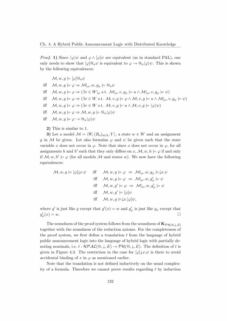
Ch. 4. A Hybrid Public Announcement Logic with Distributed Knowledge

Proof. 1) Since 〈ϕ〉ψ and ϕ ∧ [ϕ]ψ are equivalent (as in standard PAL), one

only needs to show that [ϕ]@uψ is equivalent to ϕ→ @u〈ϕ〉ψ. This is shown

by the following equivalences:

M, w, g |= [ϕ]@uψ

iff M, w, g |= ϕ⇒M|ϕ, w, gϕ |= @uψ

iff M, w, g |= ϕ⇒ (∃v ∈W |ϕ s.t. M|ϕ, v, gϕ |= u ∧M|ϕ, v, gϕ |= ψ)

iff M, w, g |= ϕ⇒ (∃v ∈W s.t. M, v, g |= ϕ ∧M, v, g |= u ∧M|ϕ, v, gϕ |= ψ)

iff M, w, g |= ϕ⇒ (∃v ∈W s.t. M, v, g |= u ∧M, v, g |= 〈ϕ〉ψ)

iff M, w, g |= ϕ⇒M, w, g |= @u〈ϕ〉ψiff M, w, g |= ϕ→ @u〈ϕ〉ψ

2) This is similar to 1.

3) Let a model M = 〈W, (Ra)a∈A, V 〉, a state w ∈ W and an assignment

g in M be given. Let also formulas ϕ and ψ be given such that the state

variable x does not occur in ϕ. Note that since x does not occur in ϕ, for all

assignments h and h′ such that they only differs on x,M, w, h |= ϕ if and only

if M, w, h′ |= ϕ (for all models M and states w). We now have the following

equivalences:

M, w, g |= [ϕ]↓x.ψ iff M, w, g |= ϕ ⇒ M|ϕ, w, gϕ |=↓x.ψiff M, w, g |= ϕ ⇒ M|ϕ, w, g′ϕ |= ψ

iff M, w, g′ |= ϕ ⇒ M|ϕ, w, g′ϕ |= ψ

iff M, w, g′ |= [ϕ]ψ

iff M, w, g |=↓x.[ϕ]ψ,

where g′ is just like g except that g′(x) = w and g′ϕ is just like gϕ except that

g′ϕ(x) = w.

The soundness of the proof system follows from the soundness of KPH(@,↓,E)

together with the soundness of the reduction axioms. For the completeness of

the proof system, we first define a translation t from the language of hybrid

public announcement logic into the language of hybrid logic with partially de-

noting nominals, i.e. t : HPAL(@, ↓, E)→ PH(@, ↓, E). The definition of t is

given in Figure 4.3. The restriction in the case for [ϕ]↓x.ψ is there to avoid

accidental binding of x in ϕ as mentioned earlier.

Note that the translation is not defined inductively on the usual complex-

ity of a formula. Therefore we cannot prove results regarding t by induction

132

4.3 Hybrid Public Announcement Logic

t(p) = p t([ϕ]p) = t(ϕ→ p)

t(u) = u 1 t([ϕ]u) = t(ϕ→ u) 1

t(¬ϕ) = ¬t(ϕ) t([ϕ]¬ψ) = t(ϕ→ ¬[ϕ]ψ)

t(ϕ ∧ ψ) = t(ϕ) ∧ t(ψ) t([ϕ]ψ ∧ χ) = t([ϕ]ψ ∧ [ϕ]χ)

t(Kaϕ) = Kat(ϕ) t([ϕ]Kaψ) = t(ϕ→ Ka[ϕ]ψ)

t(@uϕ) = @ut(ϕ) 1 t([ϕ]@uψ) = t(ϕ→ @u(ϕ ∧ [ϕ]ψ)) 1

t(↓x.ϕ) = ↓x.t(ϕ) t([ϕ]↓x.ψ) = t(↓x′.[ϕ](ψ[x := x′])) 2

t(Eϕ) = Et(ϕ) t([ϕ]Eψ) = t(ϕ→ E(ϕ ∧ [ϕ]ψ))

t([ϕ][ψ]χ) = t([ϕ ∧ [ϕ]ψ]χ)

1Where u ∈ NOM ∪ SVAR. 2x′ is a new state variable not occurring in ϕ or ψ.

Figure 4.3: The translation t : HPAL(@, ↓, E)→ PH(@, ↓, E).

on this complexity. However, the complexity of the formula immediately suc-

ceeding the public announcement operator decreases trough the translation,

and this we can use. A new complexity measure c : HPAL(@, ↓, E)→ N can

be defined such that c decreases for every step of the translation, for instance

c([ϕ]@iψ) > c(ϕ→ @i(ϕ∧ [ϕ]ψ)). The details of this are omitted, see [163] or

[105]. Using this complexity measure we can easily prove that every formula

of hybrid public announcement logic is provably equivalent to its translation:

Lemma 44. For all HPAL(@, ↓, E) formulas ϕ,

`KHPAL(@,↓,E)ϕ↔ t(ϕ).

From this lemma together with soundness of the proof system, it follows

that all formulas is also semantically equivalent to their translation:

Lemma 45. For all HPAL(@, ↓, E) formulas ϕ, all models M = 〈W,R, V 〉,all w ∈W , and all assignments g,

M, w, g |= ϕ ⇐⇒ M, w, g |= t(ϕ).

Note that translating pure formulas from HPAL(@, ↓, E) results in pure

formulas in PH(@, ↓, E). A general completeness result now follows:

Theorem 46 (Completeness for KHPAL(@,↓,E)). Let Σ be a substitution-closed

set of pure HPAL(@, ↓, E)-formulas. Every set of HPAL(@, ↓, E)-formulas

that is KHPAL(@,↓,E) + Σ-consistent is satisfiable in a model whose underlying

frame validates all the formulas in Σ.

133

Ch. 4. A Hybrid Public Announcement Logic with Distributed Knowledge

Proof. Assume that Γ is KHPAL(@ , ↓ , E) + Σ-consistent. For any set of

HPAL(@, ↓, E)-formulas X, let t(X) := {t(ϕ) | ϕ ∈ X}. Then t(Γ) is

KPH(@,↓,E)+t(Σ)-consistent, for assume otherwise: Then there are ϕ1, ..., ϕn ∈Γ such that `KPH(@,↓,E)+t(Σ) t(ϕ1∧...∧ϕn)→ ⊥. But then also `KHPAL(@,↓,E)+Σ

t(ϕ1 ∧ ... ∧ ϕn) → ⊥ (using Lemma 44 on formulas in Σ) and by Lemma 44,

`KHPAL(@,↓,E)+Σ ϕ1 ∧ ... ∧ ϕn → ⊥, which is a contradiction to Γ being

KHPAL(@,↓,E) + Σ-consistent. Now by Theorem 41 t(Γ) is satisfiable in a

model M (which is also a model for HPAL(@, ↓, E)), and by Lemma 45 it

follows that Γ is also satisfiable in M.

Finally, for all pure formulas ϕ ∈ Σ, t(ϕ) is a pure formula. Thus by

Theorem 41 the underlying frame of M validates all of the formulas t(ϕ) ∈t(Σ). But by Lemma 45 the underlying frame then also validates all ϕ ∈ Σ.

Note that we could have left out any of the operators ↓x., E, or both

and thus got completeness for any of the weaker logics. Theorem 46 also

provides completeness with respect to other classes of frames defined by pure

formulas and thus we obtain epistemic public announcement logics such as

S4HPAL(@,↓,E) and S5HPAL(@,↓,E).

4.4 Adding distributed knowledge and other modal-

ities

Often notions of group knowledge are important when modeling knowledge

in multi-agent settings. Distributed knowledge is such a notion and we will

discuss it in detail. Another is common knowledge which we will also shortly

mention. We will add distributed knowledge to KHPAL(−) in three different

ways. The first way is the standard one for public announcement logic; we

add distributed knowledge to the underlying logic KPH(−) and then give a

sound reduction axiom for distributed knowledge. Due to the generality of

Theorem 46 we also have another way of adding distributed knowledge; using

pure formulas we can add distributed knowledge directly to KHPAL(−) getting

the reduction axiom for free. The third way only works for extensions of logics

that contain satisfaction operators and the downarrow binder. In these logics

distributed knowledge becomes directly definable. The first way is a little

more involved compared to the other two, but we included it here because we

want to generalize this method to other modalities, which also give insight

into why common knowledge cannot be added to public announcement logic

using reduction axioms.

134

4.4 Adding distributed knowledge and other modalities

To add distributed knowledge we add to the given language a modal oper-

ator DB for every non-empty subset B ⊆ A. The semantics of the distributed

knowledge operator is:

M, w, g |= DBϕ iff for all v ∈W ; if (w, v) ∈⋂b∈B Rb then M, v, g |= ϕ.

The dual operator of DB will be denoted by DB. Note that the semantics of

DB is given in terms of intersection of relations, which in PDL is not modally

definable though it is axiomatizable.12 However, with nominals intersection

becomes easy to modally define (see [126] for more on these issues).

4.4.1 Adding distributed knowledge the standard way

Axioms for KPH(−,D):

All the axioms for KPH(−)

All the axioms of KPH(−) involving Ka, with Ka replaced by DB

(for every ∅ 6= B ⊆ A)

DBi↔∧b∈B Kbi, (for all i ∈ NOM and all ∅ 6= B ⊆ A) DK

Rules for KPH(−,D):

All the rules for KPH(−)

All the rules for KPH(−) involving Ka, with Ka replaced by DB

(for every ∅ 6= B ⊆ A)

Figure 4.4: The Hilbert-style proof system for KPH(−,D).

In the standard way of adding distributed knowledge we first add dis-

tributed knowledge to the language PH(−). We will use the same approach

as for the global modality: simply take the usual modal axioms and rules for

the modalities DB and add additional pure axioms. The proof system of the

logic KPH(−,D) is given in Figure 4.4. The completeness proof follows from

the general completeness in theorem 41 or 42, since the only new axiom DK

is a pure formula. All that remains to be shown is that DK defines the right

frame property. However, this is easily shown and stated as:

Lemma 47. DBi↔∧b∈B Kbi is valid on a frame 〈W, (Ra)a∈A, (RB)B 6=∅,B⊆A〉

if and only if RB =⋂b∈B Rb.

12There is no axiom that for all frames 〈W,R1, R2, R3〉 can force R1 = R2 ∩ R3, see for

instance [126]. However the logic obtained by adding distributed knowledge, interpreted as

intersection, to epistemic logic can be axiomatized, see for instance [57].

135

Ch. 4. A Hybrid Public Announcement Logic with Distributed Knowledge

Theorem 48 (Completeness of KPH(−,D)). Let Σ be a substitution-closed

set of pure PH(−, D)-formulas. Every set of PH(−, D)-formulas that is

KPH(−,D) + Σ-consistent is satisfiable in a model whose underlying frame val-

idates all the formulas in Σ.

After adding distributed knowledge to KPH(−) we can now add it to

KHPAL(−) using a reduction axiom. A reduction axiom for distributive knowl-

edge similar to the one for Ka can be used, as already noted in [157]. The ax-

iomatization of the Hybrid Public Announcement Logic, including distributed

knowledge KHPAL(−,D) is shown in Figure 4.5. The soundness of the reduction

axiom for DB is guaranteed by the following lemma:

Lemma 49. For all non-empty B ⊆ A and all HPAL(−, D)-formulas ϕ and

ψ, [ϕ]DBψ is equivalent to ϕ→ DB[ϕ]ψ.

Proof. The proof is given by the following equivalences:

M, w |= [ϕ]DBψ

iff M, w |= ϕ⇒M|ϕ, w |= DBψ

iff M, w |= ϕ⇒(∀v ∈W |ϕ

[(w, v) ∈

⋂b∈B(Rb ∩ (W |ϕ)2)⇒M|ϕ, v |= ψ

])iff M, w |= ϕ⇒

(∀v ∈W |ϕ

[(w, v) ∈ (

⋂b∈B Rb) ∩ (W |ϕ)2 ⇒M|ϕ, v |= ψ

])iff M, w |= ϕ⇒

(∀v ∈W

[M, v |= ϕ⇒

((w, v) ∈ (

⋂b∈B Rb) ∩ (W |ϕ)2 ⇒M|ϕ, v |= ψ

)])iff ∀v ∈W

[M, w |= ϕ⇒

(M, v |= ϕ⇒

((w, v) ∈ (

⋂b∈B Rb) ∩ (W |ϕ)2 ⇒M|ϕ, v |= ψ

))]iff∗ ∀v ∈W

[M, w |= ϕ⇒

(M, v |= ϕ⇒

((w, v) ∈ (

⋂b∈B Rb)⇒M|ϕ, v |= ψ

))]iff ∀v ∈W

[M, w |= ϕ⇒

((w, v) ∈ (

⋂b∈B Rb)⇒

(M, v |= ϕ⇒M|ϕ, v |= ψ

))]iff ∀v ∈W

[M, w |= ϕ⇒

((w, v) ∈ (

⋂b∈B Rb)⇒M, v |= [ϕ]ψ

)]iff M, w |= ϕ⇒ ∀v ∈W

[(w, v) ∈ (

⋂b∈B Rb)⇒M, v |= [ϕ]ψ

]iff M, w |= ϕ⇒M, w |= DB [ϕ]ψ

iff M, w |= ϕ→ DB [ϕ]ψ.

In the equivalence “iff∗” we have used the fact that (w, v) ∈ (W |ϕ)2 is equiv-

alent to M, w |= ϕ and M, v |= ϕ.

With this lemma in place we have soundness of the logic KHPAL(−,D) and

a completeness theorem for the logic, in the style of Theorem 46, can be proven

in the same way as done in Section 4.3:

136

4.4 Adding distributed knowledge and other modalities

Axioms for KHPAL(−,D):

All axioms for KPH(−,D)

All the relevant reduction axioms from Figure 4.2.

[ϕ]DBψ ↔ (ϕ→ DB [ϕ]ψ) 1 Announcement and distributed knowledge

Rules for KHPAL(−,D):

All rules for KPH(−,D)

1 Where B is a non-empty subset of A

Figure 4.5: The Hilbert-style proof system for KHPAL(@,↓,E,D).

Theorem 50 (Completeness for KHPAL(−,D)). Let Σ be a set of pure HPAL(−, D)-

formulas. Every set of HPAL(−, D)-formulas that is KHPAL(−,D)+Σ-consistent

is satisfiable in a model whose underlying frame validates all the formulas in

Σ.

4.4.2 Adding distributed knowledge directly

As the reader might have guessed, there is nothing to prevent adding dis-

tributed knowledge directly to KHPAL(@,−) using the pure formulas from the

previous subsection. In other words an alternative proof system (however re-

sulting in the same axioms and rules as the proof system of Figure 4.5) can be

described as in Figure 4.6. Completeness of this proof system follows directly

from Theorem 46. Thus we do not need to prove soundness of the reduction

axiom for DB, as it follows from the soundness of the reduction axiom for Ka.

The only thing that has to be verified in this way of adding distributed

knowledge is that we get completeness with respect to the right class of frames.

There is a little more subtleness to this than in the case of KPH(−). Theo-

rem 46 only ensures that the axiom DK becomes valid in the underlying frame

and not necessarily in all subframes of that frame. However if a frame satisfies

that RB =⋂b∈B Rb, then all subframes also satisfy this property. Thus the

meaning of DB does not change after public announcement.

To see that adding axioms that are not valid in all subframes is a real

problem, look at the modality [a; b] defined by:

M, w, g |= [a; b]ϕ iff for all v ∈W ; if (w, v) ∈ Ra;Rb then M, v, g |= ϕ,

where Ra;Rb denotes the composition of the relations Ra and Rb defined by

Ra;Rb = {(x, y) | ∃z : (x, z) ∈ Ra ∧ (z, y) ∈ Rb}. In classical Hybrid Logic

137

Ch. 4. A Hybrid Public Announcement Logic with Distributed Knowledge

Axioms for KHPAL(−,D):

All the axioms for KHPAL(−)

All the axioms of KHPAL(−) involving Ka, with Ka replaced by DB

(for every ∅ 6= B ⊆ A)

DBi↔∧b∈B Kbi, (for all i ∈ NOM and all ∅ 6= B ⊆ A) DK

Rules for KHPAL(−,D):

All the rules for KHPAL(−)

All the rules of KHPAL(−) involving Ka, with Ka replaced by DB

(for every ∅ 6= B ⊆ A)

Figure 4.6: The alternative Hilbert-style proof system for KPH(−,D).

this is definable by the pure axiom 〈a; b〉i↔ 〈a〉〈b〉i. This axiom is easily seen

to be valid exactly on the class of frames where Ra;b = Ra;Rb. However, just

because Ra;b = Ra;Rb holds on a frame, does not necessarily imply that it also

holds on all subframes.13 Thus in the scope of a public announcement operator

[ϕ] the modality [a; b] will change its meaning in the sense that it does not

quantify over the composition of the relations Ra and Rb in the submodel, but

over the composition of the relations Ra and Rb in the original model. The

problem lies in the fact that composition is not an operation that is preserved

when going to submodels contrary to intersection. We will return to this issue

in Section 4.4.4.

4.4.3 The definability of distributed knowledge using satisfac-

tion operators and the downarrow binder

In the case of the logics KPH(@,↓,−) (or KHPAL(@,↓,−)) it turns out that dis-

tributed knowledge is locally definable. The following proposition states this

formally:

Proposition 51. Let B ⊆ A contain at least 2 elements14, let a ∈ B, let ϕ

be a PH(@, ↓,−)-formula and let x and y be different state variables that do

13Take for instance the frame 〈W,Ra, Rb, Ra;b〉, where W = {x, y, z}, Ra = {(x, y)},Rb = {(y, z)} and Ra;b = {(x, z)}. Clearly this frame satisfy that Ra;b = Ra;Rb, but

in the subframe only containing the states x and z, we still have (x, z) ∈ Ra;b although

(x, z) /∈ Ra;Rb.14If B only contains b then clearly DB is definable as Kb.

138

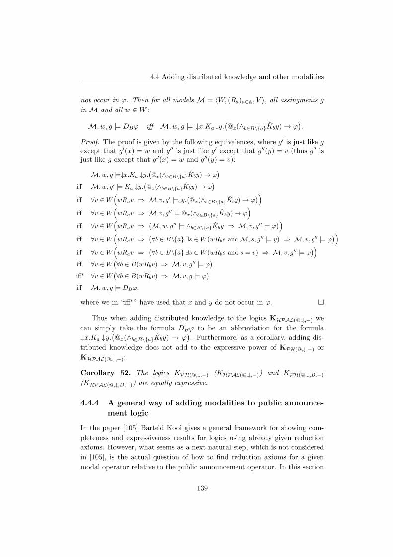
4.4 Adding distributed knowledge and other modalities

not occur in ϕ. Then for all models M = 〈W, (Ra)a∈A, V 〉, all assingments g

in M and all w ∈W :

M, w, g |= DBϕ iff M, w, g |= ↓x.Ka ↓y.(@x(∧b∈B\{a}Kby)→ ϕ

).

Proof. The proof is given by the following equivalences, where g′ is just like gexcept that g′(x) = w and g′′ is just like g′ except that g′′(y) = v (thus g′′ isjust like g except that g′′(x) = w and g′′(y) = v):

M, w, g |=↓x.Ka ↓y.(@x(∧b∈B\{a}Kby)→ ϕ

)iff M, w, g′ |= Ka ↓y.

(@x(∧b∈B\{a}Kby)→ ϕ

)iff ∀v ∈W

(wRav ⇒ M, v, g′ |=↓y.

(@x(∧b∈B\{a}Kby)→ ϕ

))iff ∀v ∈W

(wRav ⇒ M, v, g′′ |= @x(∧b∈B\{a}Kby)→ ϕ

)iff ∀v ∈W

(wRav ⇒

(M, w, g′′ |= ∧b∈B\{a}Kby ⇒ M, v, g′′ |= ϕ

))iff ∀v ∈W

(wRav ⇒

(∀b ∈ B\{a} ∃s ∈W (wRbs and M, s, g′′ |= y) ⇒ M, v, g′′ |= ϕ

))iff ∀v ∈W

(wRav ⇒

(∀b ∈ B\{a} ∃s ∈W (wRbs and s = v) ⇒ M, v, g′′ |= ϕ

))iff ∀v ∈W

(∀b ∈ B(wRbv) ⇒ M, v, g′′ |= ϕ

)iff∗ ∀v ∈W

(∀b ∈ B(wRbv) ⇒ M, v, g |= ϕ

)iff M, w, g |= DBϕ,

where we in “iff∗” have used that x and y do not occur in ϕ.

Thus when adding distributed knowledge to the logics KHPAL(@,↓,−) we

can simply take the formula DBϕ to be an abbreviation for the formula

↓x.Ka ↓y.(@x(∧b∈B\{a}Kby) → ϕ

). Furthermore, as a corollary, adding dis-

tributed knowledge does not add to the expressive power of KPH(@,↓,−) or

KHPAL(@,↓,−):

Corollary 52. The logics KPH(@,↓,−) (KHPAL(@,↓,−)) and KPH(@,↓,D,−)

(KHPAL(@,↓,D,−)) are equally expressive.

4.4.4 A general way of adding modalities to public announce-

ment logic

In the paper [105] Barteld Kooi gives a general framework for showing com-

pleteness and expressiveness results for logics using already given reduction

axioms. However, what seems as a next natural step, which is not considered

in [105], is the actual question of how to find reduction axioms for a given

modal operator relative to the public announcement operator. In this section

139

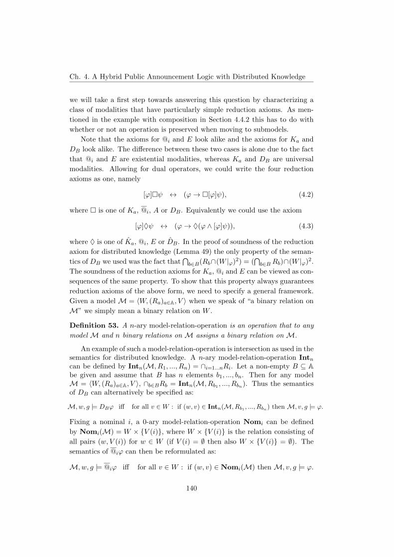
Ch. 4. A Hybrid Public Announcement Logic with Distributed Knowledge

we will take a first step towards answering this question by characterizing a

class of modalities that have particularly simple reduction axioms. As men-

tioned in the example with composition in Section 4.4.2 this has to do with

whether or not an operation is preserved when moving to submodels.

Note that the axioms for @i and E look alike and the axioms for Ka and

DB look alike. The difference between these two cases is alone due to the fact

that @i and E are existential modalities, whereas Ka and DB are universal

modalities. Allowing for dual operators, we could write the four reduction

axioms as one, namely

[ϕ]�ψ ↔ (ϕ→ �[ϕ]ψ), (4.2)

where � is one of Ka, @i, A or DB. Equivalently we could use the axiom

[ϕ]♦ψ ↔ (ϕ→ ♦(ϕ ∧ [ϕ]ψ)), (4.3)

where ♦ is one of Ka, @i, E or DB. In the proof of soundness of the reduction

axiom for distributed knowledge (Lemma 49) the only property of the seman-

tics of DB we used was the fact that⋂b∈B(Rb∩(W |ϕ)2) = (

⋂b∈B Rb)∩(W |ϕ)2.

The soundness of the reduction axioms for Ka, @i and E can be viewed as con-

sequences of the same property. To show that this property always guarantees

reduction axioms of the above form, we need to specify a general framework.

Given a model M = 〈W, (Ra)a∈A, V 〉 when we speak of “a binary relation on

M” we simply mean a binary relation on W .

Definition 53. A n-ary model-relation-operation is an operation that to any

model M and n binary relations on M assigns a binary relation on M.

An example of such a model-relation-operation is intersection as used in thesemantics for distributed knowledge. A n-ary model-relation-operation Intncan be defined by Intn(M, R1, ..., Rn) = ∩i=1...nRi. Let a non-empty B ⊆ Abe given and assume that B has n elements b1, ..., bn. Then for any modelM = 〈W, (Ra)a∈A, V 〉, ∩b∈BRb = Intn(M, Rb1 , ..., Rbn). Thus the semanticsof DB can alternatively be specified as:

M, w, g |= DBϕ iff for all v ∈W : if (w, v) ∈ Intn(M, Rb1 , ..., Rbn) then M, v, g |= ϕ.

Fixing a nominal i, a 0-ary model-relation-operation Nomi can be defined

by Nomi(M) = W × {V (i)}, where W × {V (i)} is the relation consisting of

all pairs (w, V (i)) for w ∈ W (if V (i) = ∅ then also W × {V (i)} = ∅). The

semantics of @iϕ can then be reformulated as:

M, w, g |= @iϕ iff for all v ∈W : if (w, v) ∈ Nomi(M) then M, v, g |= ϕ.

140

4.4 Adding distributed knowledge and other modalities

Similar things can be done for the semantics of E and Ka by defining

a 0-ary model-relation-operation Glo by Glo(M) = W × W and a unary

model-relation-operation Id1 by Id1(M, R) = R. Further examples of model-

relation-operations are the PDL constructors union (∪), composition (;) and

transitive closure (∗).

Definition 54. An n-ary model-relation-operation F respects intersection if

for all models M, all relations R1, ..., Rn on M and any C ⊆W ×W :

F(M, R1 ∩ C, ..., Rn ∩ C) = F(M, R1, ..., Rn) ∩ C.

Note, that all of the model-relation-operations Intn, Nomi, Glo and Id

respect intersection (this is easy to see). This is also the case for the PDL

constructor union, but not for the composition and transitive closure.15

The property of respecting intersection is the right property to ensure

simple reduction axioms. However, before we can state this we need to add

modalities based on model-relation-operations to the syntax of the language.

To do this we assume a set of function symbols FSYM (all F ∈ FSYM is

assumed to have a finite arity) which we use to refer to the model-relation-

operations. Since these operations also take relations as argument, we need

something to fill in as arguments in the function symbols and for this we use

the set of agents A already given. Now to the syntax of our languages PH(−)

and HPAL(−), we add a new modal operator [F (a1, ..., an)] for each n-ary

function symbol F ∈ FSYM and each a1, ..., an ∈ A.

To give semantics for the new modalities we need to interpret the function

symbols. For this we assume a relation-interpretation I that assigns an n-ary

model-relation-operation I(F ) to each F ∈ FSYM of arity n. With this fixed

relation-interpretation I we can define the semantics of the new modalities

by:

M, w, g |= [F (a1, ..., an)]ϕ

iff for all v ∈W : if (w, v) ∈ I(F )(M, Ra1 , ..., Ran

)then M, v, g |= ϕ.

(4.4)

Modalities defined using model-relation-operations that respect intersec-

tion have very simple reduction axioms in the form of (4.2) and (4.3). How-

ever, one cannot just add these reduction axioms to get a sound and complete

15In the case of the composition constructor take for instance W = {x, y, z}, Ra = {(x, y)}and Rb = {(y, z)}. Then Ra;Rb = {(x, z)} and thus (Ra;Rb) ∩ {x, z}2 = {(x, z)}. But

Ra ∩ {x, z}2 = ∅ and Rb ∩ {x, z}2 = ∅, so (Ra ∩ {x, z}2); (Rb ∩ {x, z}2) = ∅.

141

Ch. 4. A Hybrid Public Announcement Logic with Distributed Knowledge

logic, there has to be a sound and complete axiom system for the underly-

ing logic as well (in some cases, such as distributed knowledge, this is easy

since the modality is definable by pure formulas). But with this in mind our

considerations can be summarized in the following proposition:

Proposition 55. Let F ∈ FSYM be of arity n and such that I(F ) respects

intersection and let a1, ..., an ∈ A. Assume furthermore that there is a sound

and complete axiom system for the logic KPH(−,[F (a1,...,an)]), then a sound and

complete axiom system for the logic KHPAL(−,[F (a1,...,an)]) can be obtained by

adding the reduction axiom

[ϕ][F (a1, ..., an)]ψ ↔ (ϕ→ [F (a1, ..., an)][ϕ]ψ)

(together with the other relevant reduction axioms) to the axiom system of

KPH(−,[F (a1,...,an)]). Furthermore the logic KHPAL(−,[F (a1,...,an)]) is no more

expressive than KPH(−,[F (a1,...,an)]).

Proof. The proof is similar to the proof of Theorem 50 based on a rewriting of

the proof of Lemma 49 using the assumption that I(F ) respects intersection.

This proposition gives a uniform way of adding @i, E and DB to the

logic KHPAL(−). Furthermore since the PDL operator “∪” also respects in-

tersection, the epistemic modality EB reading “everybody amongst B knows

that...” can also be added with a reduction axiom of the form [ϕ]EBψ ↔ (ϕ→EB[ϕ]ψ).16 Since the operator of composition does not respect intersection,

we do not obtain a reduction axiom in the style of the ones for DB or EB.

We have presented the proposition as an extension of KHPAL(−), however,

it is clear that it works for any extension of just classical PAL (without com-

mon knowledge). Another important remark is that we have presented the

proposition in the setting of the basic logic K, and it cannot just be extended

to arbitrary extensions of K. If we require that the relations (Ra)a∈A of our

models satisfy a certain property (like reflexivity or transitivity etc.), we can-

not always be sure that the restricted relations Ra ∩ (W |ϕ)2 also satisfy this

property. Thus if the property is not preserved when taking intersection the

proposition does not apply. Nevertheless, if it is preserved we can extend the

result beyond K. One example is assuming that all the relations Ra for a ∈ A16Note, however, that since EBϕ is directly definable as

∧b∈B Kbϕ, it is not necessary to

have the modality explicit in the language as in the case of distributed knowledge in the

logic KPH(@,↓,−).

142

4.5 Conclusion and further work

are equivalence relations, which is normally done in Epistemic Logic. Here

there is no problem since restricting an equivalence relation Ra to Ra∩(W |ϕ)2

gives rise to an equivalence relation. Finally, note that the proposition only

provides sufficient and not necessary conditions for the existence of reduction

axioms. Finding necessary conditions is left for further research.

4.4.5 A note on common knowledge

We now turn to common knowledge. For a non-empty subset B ⊆ A, thecommon knowledge operator CB is added to the language, with the readingof CBϕ as “it is common knowledge among the agents in B that ϕ”. CB hasthe following semantics:

M, w, g |= CBϕ iff for all v ∈W ; if (w, v) ∈(⋃

b∈B Rb

)∗then M, v, g |= ϕ,

where R∗ denotes the reflexive transitive closure of the relation R.

Problems arise when one wants to combine public announcement logic with

common knowledge in the sense that we cannot prove completeness using re-

duction axioms anymore. Reduction axioms for common knowledge simply

do not exist. One solution is to generalize the notion of common knowledge

to what is called relativized common knowledge. Relativized common knowl-

edge is exactly the notion needed to get completeness via reduction axioms

for public announcement, see [157]. We will not take on the enterprise of

adding common knowledge or relativized common knowledge to KPH(−) or

KHPAL(−). We simply mention common knowledge because the concept of

respecting intersection makes it clear why reduction axioms such as the ones

for Ka, E and DB do not work for common knowledge. Common knowledge

corresponds to the PDL operator of transitive closure, which does not respect

intersection and cannot otherwise be defined.

4.5 Conclusion and further work

In this paper it has been shown that nominals, satisfaction operators, the dow-

narrow binder, the global modality, and distributed knowledge can be added

to the Public Announcement Logic. Furthermore general completeness results

for extensions with pure formulas, a well celebrated result in Hybrid Logic,

also transfer to the case of Hybrid Public Announcement Logic. Properties of

both Hybrid Logic and Public Announcement Logic are thus preserved in the

combination. The completeness is shown using reduction axioms as in classical

Public Announcement Logic. Hence the public announcement operator does

143

Ch. 4. A Hybrid Public Announcement Logic with Distributed Knowledge

not increase the expressive power when added to Hybrid Logic. Using the

terminology of [154], classical Hybrid Logic is not closed under relativization

because nominals might lose their references in submodels, but relaxing Hy-

brid Logic to a logic with only partially denoting nominals, Hybrid Logic does

become closed under relativization. Thus, the fact that the [ϕ]-operator does

not add expressivity is preserved in hybrid extensions of the basic multi-modal

logic.

That the nice properties of Hybrid Logic are preserved in the combina-

tion with Public Announcement Logic adds significantly to the proof theory

of Public Announcement Logic. We have demonstrated this by adding dis-

tributed knowledge via pure formulas. It was also shown that distributed

knowledge could actually be defined using satisfaction operators and the dow-

narrow binder. That Hybrid Logic has much to offer the proof theory of Public

Announcement Logic is also demonstrated by the tableau system developed

in [80], but surely there is still much more that Hybrid Logic can offer to

the proof theory of Public Announcement Logic. This is left for future re-

search. Finally a sufficient requirement for the existence of reduction axioms

in a general setting has been discussed. This naturally leads to the question

of whether there is a semantic requirement to put on the operations of section

4.4 that exactly characterizes the operations that allow reduction axioms. We

leave this as further work as well.

Another line of further research is to add common knowledge to the Hybrid

Public Announcement Logic. However, as mentioned, this might not allow

completeness via reduction axioms. Besides adding common knowledge there

is also the question of extending the logic from Public Announcement Logic

to full Dynamic Epistemic Logic. The problem here is that in full Dynamic

Epistemic Logic there are epistemic actions that can expand a state into several

states, and thus it is not clear anymore what nominals should denote.

Acknowledgment

This paper has occurred in many draft versions and several people have com-

mented on various versions among others Olivier Roy, Jiahong Guo, Mai

Ajspur, and Sine Zambach. The participants of the ILLC seminar on Log-

ics for Dynamics of Information and Preferences 2009, the participants of the

HYLOCORE 2009 workshop, and the participants of the HyLo 2010 work-

shop have also provided useful comments on presentations of this work. A

special thanks to Torben Brauner for many useful comments and suggestions

144

4.6 Appendix: Alternative semantics for the public announcement operator

on all the versions of the paper. Finally, I would like to thank a number of

anonymous reviews for very useful comments.

The author is partially funded by the Danish Natural Science Research

Council through the HYLOCORE project.

4.6 Appendix: Alternative semantics for the public

announcement operator

In this section we discuss the relationship between the standard semantics and

an alternative semantics for the public announcement operator.

Let us first fix the terminology. The semantics already introduced will be

referred to as the standard semantics. By the alternative semantics we refer

to the semantics of classical hybrid logic together with the following semantics

for the public announcement operator [ϕ]:

M, w |= [ϕ]ψ ⇐⇒ M, w |= ϕ implies that M|ϕ, w |= ψ,

where M|ϕ is the model M = 〈W, (Ra|ϕ)a∈A, V 〉, where

Ra|ϕ = Ra ∩ ({w ∈W | M, w |= ϕ} × {w ∈W | M, w |= ϕ}).

For the global modality it is easy to see that the logic obtained with the

alternative semantics differs from the standard one. In the standard semantics

the formula [p]Ap is valid, but with the alternative semantics it is no longer

valid. In a similar way we have that [p]E¬p becomes satisfiable. So after

updating with the fact p there is still a state where p is false, which seems

contra intuitive. In general publicly announcing a formula involving higher

order knowledge might lead to it becoming false, but p is a propositional fact

about the worlds which normally are assumed to be unchangeable by just

announcements. This is also so in classical PAL. Thus when including the

global modality it is more reasonable to use the standard semantics for the

public announcement operator.

With the alternative semantics the satisfaction operator also get strange

properties. Before an announcement it might be the case that @ip∧@i¬Kap,

i.e. agent a does not know p at the state i. However, after announcing that the

actual state is not i (i.e. a public announcement of ¬i) it becomes true that

@iKap in the alternative semantics. This is essentially due to the following

validity in the alternative semantics: [¬i](@iϕ → @iKaϕ). Thus information

about which state is not the case gives complete information about the world

145

Ch. 4. A Hybrid Public Announcement Logic with Distributed Knowledge

at that state to every agent. Note that in the standard semantics announcing

¬i simply makes every formula of the form @iϕ false, which may not be a

completely pleasing solution, but still the best one to the authors opinion.

Comparing the two logics related to the two semantics, note that [p]Ap is

valid in the standard semantics but not in the alternative one. On the other

hand Ep→ [ϕ]Ep is valid in the alternative semantics, but not in the standard

one. Thus the two logics are simply different; none of them are contained in

the other. Furthermore, and also important, it does not seem entirely clear

how to derive reduction axioms for the logic of the alternative semantics.

146

Chapter 5

Terminating tableaux for dynamic

epistemic logics

Published in Electronic Notes in Theoretical Computer Science 262:

141–156, 2010. Proceedings of the 6th Workshop on Methods for

Modalities (M4M-6 2009).

Abstract: Throughout the last decade, there has been an in-

creased interest in various forms of dynamic epistemic logics to

model the flow of information and the effect this flow has on knowl-

edge in multi-agent systems. This enterprise, however, has mostly

been applicationally and semantically driven. This results in a

limited amount of proof theory for dynamic epistemic logics.

In this paper, we try to compensate for a part of this by presenting

terminating tableau systems for full dynamic epistemic logic with

action models and for a hybrid public announcement logic (both

without common knowledge). The tableau systems are extensions

of already existing tableau systems, in addition to which we have

used the reduction axioms of dynamic epistemic logic to define

rules for the dynamic part of the logics. Termination is shown

using methods introduced by Brauner, Bolander, and Blackburn.

Keywords: Dynamic epistemic logic, public announcement logic,

terminating tableau systems, decision procedures, hybrid logic, re-

duction axioms.

147

Ch. 5. Terminating tableaux for dynamic epistemic logics

5.1 Introduction

Classic epistemic logic has played an important role in both philosophy and

computer science. However, recent years have witnessed the importance of

also looking at the dynamics of knowledge, i.e. how knowledge of different

agents can change due to the development of a system. There are two ways

of adding dynamics to epistemic logic. One can either combine it with a

temporal logic or combine it with some dynamic logic of actions. The latter

approach has become increasingly common and has resulted in what is now

called Dynamic Epistemic Logic (DEL), which includes operators for so called

epistemic actions (cf. [163]). The interest in DEL has mostly been related to

applications, and has mainly been semantically driven. Thus, only very few

attempts to develop a rich proof theory for DEL beyond standard Hilbert style

systems have been performed. This work attempts to make up for some of

this by discussing terminating tableau systems for different kinds of dynamic

epistemic logics.

The simplest form of dynamics one can add to classical epistemic logic is

a public announcement operator. The language is extended with formulas of

the type [ϕ]ψ, which are read as “after public announcement of ϕ, ψ holds”.

At the semantic level, the operator [ϕ] corresponds to moving to the submodel

consisting only of states where ϕ is true (thus we are exclusively concerned with

truthful public announcements here). This simple extension, called Public

Announcement Logic (PAL), is, nevertheless, quite useful as shown by the

many applications presented in [163]. Having left out common knowledge,

operators1, this logic is fairly simple and a few tableau systems do already

exist, see [14] and [49]. The approach in this paper is different from these in

the sense that we try to avoid constructing new complicated and tailor made

tableau systems by instead using the existing systems. This is possible due to

reduction axioms. Reduction axioms have, from the beginning of DEL’s short

history, played an important role in showing completeness and expressiveness

results. It was proved that Public Announcement Logic is no more expressive

than the underlying epistemic logic. Using reduction axioms, it is possible to

translate a public announcement formula into an equivalent one without any

public announcement operators.

There are a lot of other possible epistemic actions, moving beyond bare

public announcements: announcements to subgroups, private communications,

1In the rest of this paper, at least until the conclusion, we will disregard common knowl-

edge.

148

5.1 Introduction

secret announcements and more. The insight of Baltag, Moss and Solecki (in

[15]) is that all these epistemic actions, considered as action modalities, can

also be represented by a form of Kripke models. Using a general product

operation on Kripke models, they can be given a semantic. More surprisingly,

it was shown that also formulas with these more complicated action modalities

can be reduced to basic epistemic formulas without any action modalities.

This, of course, required more advanced reduction axioms than in the case of

public announcements.

When one wants to prove a validity of DEL, one can simply translate the

validity into an epistemic formula without action modalities and then use the

existing tableau (or other) systems. However, the translation might result in

an exponential increase in the size of the formula. As is shown in [115], this

exponential increase cannot be avoided for public announcements. This fact

provides another motivation for using DEL, since it offers us the opportunity

to express things much more compactly than in classical epistemic logic. It

is also shown in [115] that the complexity of validity checking for PAL is

no higher than for the underlying epistemic logic. Thus, the method of first

translating and then using known proof methods for classical epistemic logic

may be unfeasible. This justifies the direct tableau systems for PAL given in

[14] and [49]. In DELs with arbitrary epistemic actions, the matter becomes

much more complicated. Here, the challenge is how to represent the action

modalities. Since PAL is part of DEL, [115] also shows that the blowup of

the translation may be exponential in the general DEL case. However, it is

currently unknown to the author exactly what the complexity of deciding DEL

validities is.2 When adding the global modality to the underlying epistemic

logic, the complexity of this will already be exponential [144]. In this case, the

exponential increase caused by the translation therefore does not destroy the

worst-case complexity.

The work in this paper is based on the idea of using reduction axioms as

rules to make the translation on the fly in the tableaux. In practice, this is

more efficient than performing the whole translation at the beginning3, but in

2When dealing with arbitrary formulas of DEL, the question is how to measure the size

of the action modalities. On the one hand, an action modality could be counted as one

symbol, but when deciding validity, the finer structure of the action modality is needed.

Thus, this may result in a high complexity for validity checking in this size of the formula.

On the other hand, using another size-measure of action modalities, it may become possible

to decide validity in lower complexity in that size.3In worst case scenario doing the translation on the fly may not be more efficient. But

there seems to be at least two cases where translation on the fly will speed up the process

149

Ch. 5. Terminating tableaux for dynamic epistemic logics

the case of public announcement, it might not be as fast as the methods of [14]

and [49]. However, their tableau systems only work for public announcement

logic, while the method presented here further works for full dynamic epistemic

logic and for a hybrid version of public announcement logic. Our tableaux in

this paper are kept terminating using the methods of Brauner, Bolander, and

Blackburn ([38], [39], and [37]). The presentation here will be based on the

approach in [37]. For basic modal logic, they show termination by noticing that

the maximal formula complexity drops as new prefixes are introduced, which

makes infinite tableaux impossible. In this paper we show that, essentially,

this argument can be adapted in the setting where reduction axioms are used

as extra tableau rules.

The paper is structured as follows: first we introduce public announcement

logic, a hybrid public announcement logic, and full dynamic epistemic logic

(Section 5.2). Then, we present a terminating tableau system for full dynamic

epistemic logic in Section 5.3. Following this, we demonstrate how the ap-

proach can also be used to create a terminating tableau system for the hybrid

public announcement logic. Finally, we present some concluding remarks and

discuss further research.

5.2 Dynamic epistemic logic

We will first present the formal definitions of public announcement logic. Pub-

lic announcements are added to the normal modal logic K, but it can easily

be extended to the case of S5, which is often used for modeling knowledge.

We will leave out common knowledge. First, we assume a finite set of agents

A and a countable infinite set of propositional variables PROP. Using the

terminology of [163] the language of the Public Announcement Logic will be

denoted by LK[], and is given by the following syntax:

ϕ ::= p | ¬ϕ | ϕ ∧ ϕ | Kaϕ | [ϕ]ϕ,

where p ∈ PROP and a ∈ A. The connectives ∨, → and ↔ are defined

from ¬ and ∧ in the usual way, and the dual operators ¬Ka¬ and ¬[ϕ]¬ are

abbreviated by Ka and 〈ϕ〉. The interpretation of Kaϕ is that “agent a knows

of deciding a formula. The first case is where only few steps of translation are needed

to detect an inconsistency, as for instance in the formula [¬[¬(q ∧ r)]Ka(p → q)](p ∨ r) ∧¬ ((¬[¬(q ∧ r)]Ka(p→ q))→ (p ∨ r)). The other case is where the need for a translation

may only occur at the very end of the tableau construction process, as for instance in the

formula Ka[p]p ∧ ¬Ka¬[q]¬q ∧Ka([q]p ∧ [p]q).

150

5.2 Dynamic epistemic logic

that ϕ” and of [ϕ]ψ that “after (truthful) public announcement of ϕ, ψ is the

case”. These interpretations are captured by the following formal semantic:

A Kripke frame (or just a frame) is a pair F = 〈W, (Ra)a∈A〉 consisting of a

non-empty set W of states (or possible worlds) and for each a ∈ A a binary

relation Ra on W (i.e. Ra ⊆ W × W ). A model M is a pair consisting

of a frame F and a valuation V that assigns a set of states in W to every

propositional variable of PROP (i.e. V : PROP→ P(W )). Given a formula ϕ

of LK[], a model M = 〈w, (Ra)a∈A, V 〉, and a state w ∈ W , the truth of ϕ at

w, notation M, w |= ϕ, is defined as standard in modal logic, taking Ka to

be the box modality corresponding to Ra. In addition we add the following

clause for [ϕ]ψ:

M, w |= [ϕ]ψ iff M, w |= ϕ implies that M|ϕ, w |= ψ,

where the model M|ϕ = 〈W |ϕ, R|ϕ, V |ϕ〉 is defined by:

W |ϕ = {v ∈W | M, v |= ϕ}Ra|ϕ = Ra ∩ (W |ϕ ×W |ϕ)

V |ϕ(p) = V (p) ∩W |ϕ.

We write M |= ϕ if M, w |= ϕ for all w ∈ W and we say that ϕ is valid if

M |= ϕ for all models M. The logic of this semantic will be denoted by PA

and be call Public Announcement Logic. It is not hard to prove the following

validities in this logic:

[ϕ] p ↔ (ϕ→ p) (5.1)

[ϕ]¬ψ ↔ (ϕ→ ¬[ϕ]ψ) (5.2)

[ϕ] (ψ ∧ χ) ↔ ([ϕ]ψ ∧ [ϕ]χ) (5.3)

[ϕ]Kaψ ↔ (ϕ→ Ka[ϕ]ψ) (5.4)

[ϕ] [ψ]χ ↔ [ϕ ∧ [ϕ]ψ]χ. (5.5)

These are the reduction axioms for public announcement [163]. Adding these

axioms together with necessitation of [ϕ] to a Hilbert style proof system for

multi modal K will result in a sound and complete proof system for PA (for

details see [163]).

Note that the complexity of the formula occurring within the scope of the

public announcement operator is greater on the left than on the right side

of “↔” in these reduction axioms. This can be used to define a translation

T : LK[] → LK , where LK is the standard multi-modal language. The trans-

lation “commutes” with all logic operators beside the public announcement

151

Ch. 5. Terminating tableaux for dynamic epistemic logics

operator (e.g. T (¬ϕ) = ¬T (ϕ)). In the case when the translation encounter a

[ϕ] operator it uses the reduction axioms to decrease the complexity of the for-

mula within the scope of the operator, e.g. T ([ϕ](¬ψ)) = T (ϕ) → ¬T ([ϕ]ψ).

This translation can be shown to be a truth preserving translation of PA into

multi modal K, which shows that adding the public announcement operator

does not increase the expressiveness of the language.4 This recursive trans-

lation is not recursive in the normal way, since going from left to right (of

↔) in the reduction axioms (5.1)–(5.5) does not reduce the standard formula

complexity. Therefore, to prove the correctness of the translation, a new com-

plexity measure on the formulas is needed. One possible measure is (taken

from [163]):

Definition 56. Define a complexity measure c : LK[] → N by the inductive

clauses:c(p) = 1

c(¬ϕ) = 1 + c(ϕ)

c(ϕ ∧ ψ) = 1 + max{c(ϕ), c(ψ)}c(Kaϕ) = 1 + c(ϕ)

c([ϕ]ψ) = (4 + c(ϕ)) · c(ψ)

What can be shown about this complexity measure is that it decreases

when moving to subformulas and, furthermore, that the c complexities of

the left hand sides of the reduction axioms (5.1)–(5.5) are higher than the c

complexities of the right hand sides. This fact will be important when we

consider the tableau system in the next section.

We will not present a tableau system for PA, but for a hybrid extension

of this, namely the Hybrid Public Announcement Logic of [81] (Chapter 4).

To obtain this new logic we will first extend the language. For this we fix a

countable infinite set of nominals NOM disjoint from the propositional vari-

ables. The language of hybrid public announcement logic LHPA is defined

by:

ϕ ::= p | i | ¬ϕ | ϕ ∧ ϕ | Kaϕ | [ϕ]ϕ | @iϕ | Eϕ,4This also works when the underlying logic is S5, however, if one wants to models beliefs

using the logic KD45 a problem arise. The problem is that the frame properties defined

by the axioms of KD45 are not preserved under the operation of taking submodels. Thus

one cannot get completeness with respect to the class of models where beliefs are always

interpreted as KD45. In other words the given semantic for the public announcement

operator can result in agents having inconsistent beliefs after a public announcement.

152

5.2 Dynamic epistemic logic

where p ∈ PROP, i ∈ NOM and a ∈ A.

The nominals will function as names for states. The formula @iϕ states

that ϕ is true at the state that i denotes and Eϕ express that there is a

state where ϕ is true. The semantics is specified somewhat different from

what is standard in hybrid logic. The reason is that the semantic of the

public announcement operator takes us to submodels where states denoted by

nominals may disappear. To deal with this, we extend the class of models such

that the valuation assigns at most one state instead of exactly one state to each

nominal (for more on these issues, see [81]). The definition of a model M =

〈W, (Ra)a∈A, V 〉 is thus the same as for PA, but with the further requirement

on the valuation V : PROP ∪ NOM→ P(W ) that |V (i)| ≤ 1 for all i ∈ NOM.

For the part of the language that coincide with LK[] the semantic clauses are

the same as for PA. For the new part of the language we define:

M, w |= i iff w ∈ V (i)

M, w |= @iϕ iff there is a v ∈ V (i) such that M, v |= ϕ

M, w |= Eϕ iff there is a v ∈W such that M, v |= ϕ.

The logic, this semantic give rise to, will be called “Hybrid Public Announce-

ment Logic” and will be denoted by HPA. The dual operators of E and

@i will be denoted by A and @i. Note, that since nominals only partially

denote states, @i is no longer its own dual. We still have the equivalences

@iϕ ≡ E(i ∧ ϕ) and @iϕ ≡ A(i → ϕ) though, but now these might not be

equivalent anymore.5 Thus the satisfaction operator has been split into an

existential quantifier @ and an universal one @. The fact, that the nominal i

denotes something in a model (i.e. |V (i)| = 1) can be expressed by the formula

Ei.

Completeness with respect to a Hilbert style proof system can also be

shown using reduction axioms, as the following from [81]:

[ϕ] i ↔ (ϕ→ i) (5.6)

[ϕ] @iψ ↔ (ϕ→ @i(ϕ ∧ [ϕ]ψ)) (5.7)

[ϕ]Eψ ↔ (ϕ→ E(ϕ ∧ [ϕ]ψ)) (5.8)

Since we extended the language of LK[] we also need to extend the definition

5These equivalences also show that we do not need the @i operator in the language, since

it is definable in terms of E and i. However to ease the adaption of the tableau system from

[37] we keep @i in the language.

153

Ch. 5. Terminating tableaux for dynamic epistemic logics

of the measure c. This done by adding the following clauses to Definition 56:

c(i) = 1

c(@iϕ) = 1 + c(ϕ)

c(Eϕ) = 1 + c(ϕ).

With this complexity measure, the left hand sides of the new reduction axioms

(5.6)–(5.8) still have higher c complexity than the right hand sides.

Public announcements are just one kind of epistemic action though. To deal

with a larger amount of epistemic actions in a uniform way, the notion of

action models was introduced by Baltag, Moss and Solecki [15]. The intuition

behind epistemic action models is that the agents may be unsure about ex-

actly which action takes place and that each action has a precondition that

has to be satisfied for that action to take place. Epistemic actions can be rep-

resented by Kripke structures where each state is an event/action and instead

of a complete valuation each event is assigned a formula of the language as a

precondition.

We now turn to the formal details. An action model M = 〈S, (Qa)a∈A, pre〉consists of a finite set of events S, accessibility relations Qa on S for all agents

a ∈ A, and a precondition function pre : S → L assigning a precondition to

every event (for some logical language L). The language of formulas, LK⊗,

and the action model language, LactK⊗, have to be defined at the same time

using mutual recursion. The action model language LactK⊗ is defined by:

α ::= (M, s),

where M = 〈S, (Qa)a∈A, pre〉 is an action model such that s ∈ S and pre : S→LK⊗. At the same time the formula language LK⊗ is defined by:

ϕ ::= p | ¬ϕ | ϕ ∧ ϕ | Kaϕ | [α]ϕ,

where p ∈ PROP, a ∈ A, and α ∈ LactK⊗.6 The reading of the formula [M, s]ϕ is

“after the epistemic action (M, s), ϕ is the case”. M represent the uncertainty

among the agents about what event is taking place, and s is the event that

actually takes place.

6By this definition we load the syntax of the language with heavy semantic machinery,

however, since we only deal with finite action models it is possible to list and name them

all. For more on this discussion see [163].

154

5.2 Dynamic epistemic logic

For general epistemic actions a little contemplation shows that they can

actually result in an enlargement of a Kripke model. The way we reflect this in

the semantic is by defining a product update between a Kripke model and an

action model. For a Kripke modelM = 〈W, (Ra)a∈A, V 〉 and an action model

M = 〈S, (Qa)a∈A, pre〉 define the restricted productM⊗M = 〈W ′, (R′a)a∈A, V ′〉by:

W ′ = {(w, s) ∈M×M | M, w |= pre(s)}R′a((w, s), (v, t)

)iff Ra(w, v) and Qa(s, t)

V ′(p) = {(w, s) ∈W ′ |w ∈ V (p)}.

We can now define the semantic of the action modality [M, s] as:

M, w |= [M, s]ϕ iff M, w |= pre(s) implies that M⊗M, (w, s) |= ϕ.

The other logical operators have the normal semantic and validity is also

defined in the standard way. This logic will be called Dynamic Epistemic Logic

and be denoted by AM. Note that we have now left out the hybrid machinery

since it is not obvious how exactly to combine it with action models.7

As in the case of public announcement, adding action modalities does not

increase the expressive power of the language. Again this is shown by providing

reduction axioms (see for instance [163]). The reduction axioms, which are

now a little more complex, are:

[M, s] p ↔(pre(s)→ p

)(5.9)

[M, s]¬ϕ ↔(pre(s)→ ¬[M, s]ϕ

)(5.10)

[M, s] (ϕ ∧ ψ) ↔([M, s]ϕ ∧ [M, s]ψ

)(5.11)

[M, s]Kaϕ ↔(pre(s)→

∧Ra(s,t)

Ka[M, t]ϕ)

(5.12)

[M, s] [M′, s′]ϕ ↔ [(M; M′), (s, s′)]ϕ, (5.13)

where, in the last formula ,the “;” operation is a semantic operation on ac-

tion models. Given two action models, M = 〈S, (Qa)a∈A, pre〉 and M′ =

7The interpretation of nominals is none obvious when modalities capable of expanding

states are present. Normally, nominals in hybrid logic are a special kind of propositional

variables, which are true in exactly one state. However, when taking a product of an epistemic

model with an action model, single states of the epistemic model can turn into several states

in the resulting product model. Thus, if one keeps the original definition of the valuation

for the product model, one breaks the requirement of nominals only being true in one state.

On the other hand, there seems to be no obvious alternative definition of the valuation.

155

Ch. 5. Terminating tableaux for dynamic epistemic logics

〈S′, (Q′a)a∈A, pre′〉, the composition (M; M′) = 〈S′′, (Q′′a)a∈A, pre′′〉 is defined by:

S′′ = S× S′

Q′′a((s, s′), (t, t′)

)iff Qa(s, t) and Q′a(s′, t′)

pre′′((s, s′)) = 〈M, s〉pre′(s′).

See [163] for the validity of the reduction axioms. As for HPA a new

complexity measure is needed. A such, taken from [163], is:

Definition 57. The complexity measure d : LK⊗ → N is defined inductively

by:

d(p) = 1

d(¬ϕ) = 1 + d(ϕ)

d(ϕ ∧ ψ) = 1 + max{d(ϕ), d(ψ)}d(Kaϕ) = 1 + d(ϕ)

d([M, s]ϕ) =(4 + d(M, s)

)· d(ϕ)

d(M, s) = max{d(pre(t)) | t ∈ M}.

As for public announcement it can be shown that this complexity measure

decreases when moving from the left hand sides to the right hand sides (of↔)

of the reduction axioms (5.9)–(5.13), as well as when moving to subformulas.

5.3 A tableaux system for AM

In this section we introduce a tableau system for AM built on an existing

tableau system for multi modal K, where we add the reduction axioms as

tableau rules. This is done without violating termination or completeness of

the original system. Formally, we will take a tableau to be a finitely branching

tree, where each node is labeled by a formula of our language. As basic tableau

system for the underlying multi modal K logic we will use the one from [37],

which is a standard one.8 The tableau system is a prefixed tableau system,

thus all formulas occurring on the tableaux have the form σϕ, where σ comes

from some fixed countable infinite set of prefixes. The intuition behind the

prefixes is that they represent states in a possible Kripke model. Thus the

intuition behind σϕ is that ϕ holds at σ. Additionally, we also have formulas

of the form σRaτ on the tableaux representing that τ is accessible from σ by

8The tableau system of [37] is also shown in Figure 1.5 of Section 1.2.1. The only change

we have made to that system is the addition of the rules ([AM ]) and (¬[AM ]).

156

5.3 A tableaux system for AM

σ¬¬ϕ(¬¬)

σϕ

σϕ ∧ ψ(∧)

σϕ

σψ

σ¬(ϕ ∧ ψ)(¬∧)

σ¬ϕ σ¬ψ

σ¬Kaϕ(¬Ka)

1

σRaτ

τ¬ϕ

σKaϕ σRaτ(Ka)

τϕ

σ[M, s]ϕ([AM ])

σt([M, s]ϕ)

σ¬[M, s]ϕ(¬[AM ])

σ¬t([M, s]ϕ)

1 The prefix τ is new to the branch.

Figure 5.1: Tableau rules AM.

agent a. These will be called accessibility formulas. The rules of the tableau

system applies to branches of tableaux and are presented in Figure 5.1.

In the rules ([AM ]) and (¬[AM ]), t is the operation that uses the reduc-

tion axioms to translate the formula [M, s]ϕ to a formula of less d-complexity.

For instance t([M, s](ϕ ∧ ψ)) = [M, s]ϕ ∧ [M, s]ψ.9 Ignoring the accessibility

formulas, the formula above the line in a rule will be called the premise and

the formula(s) below the line the conclusion(s). When constructing a tableau,

we never add a formula to a branch if it already occurs on the branch, and we

never apply the (¬Ka) rule twice to the same formula on a branch. If a branch

contains both σϕ and σ¬ϕ for some formula ϕ and some prefix σ, then the

branch is called closed, otherwise open. A closed tableau is one in which all

branches are closed. A tableau proof of a formula ϕ is a closed tableau with

σ¬ϕ as the root formula.

5.3.1 Termination of the tableau system

Two important properties for ensuring termination in the work of [37] are; all

formulas occurring on the tableau are subformulas or negation of subformulas

of the root formula, and every rule only generates something of less formula

complexity. These two properties are essential for ensuring finiteness of the

tableaux. However, these properties fail for our tableau system because the

rules ([AM ]) and (¬[AM ]) can generate formulas that are not subformulas of

9t is not to be confused with a full translation for the language LK⊗ as discussed in

Section 5.2. Here t only translate/reduces one level.

157

Ch. 5. Terminating tableaux for dynamic epistemic logics

the premise and may have higher formula complexity. But using the notion of

d-complexity and stretching the notion of a subformula we can retain finiteness.

Before a new notion of subformula can be defined a lemma is needed. For an

action model M = 〈S, (Qa)a∈A, pre〉, let D(M) denote the domain, i.e. D(M) =

S.

Lemma 58. Let σ0ϕ0 be the root formula of a tableau T and assume that

[M, s]ϕ occurs on T . Then, there are an n ≤ d(ϕ0) and action models M1, ...,Mn

occurring in ϕ0, such that D(M) = D(M1)× ...×D(Mn).

Proof. The proof goes by induction on the construction of T . The claim is

obvious for [M, s]ϕ being ϕ0. It is also obvious that when applying any rule,

besides ([AM ]) and (¬[AM ]) applied to formulas of the form [M, s][M′, s′]ψ and

¬[M, s][M′, s′]ψ, the action modalities in the conclusions and the premises have

the same domains (or the action modality have completely been removed).

Now for the rules ([AM ]) and (¬[AM ]) applied to two consecutive modalities

[M, s] and [M′, s′]. Assume that the claim of the lemma is true for [M, s] and

[M′, s′]. Then

D(

(M; M′), (s, s′))

= D(M1)× ...×D(Mn)×D(M′1)× ...×D(M′m), (5.14)

where Mi and M′j occur in ϕ0 for all 1 ≤ i ≤ n and 1 ≤ j ≤ m. Thus, the

only thing that remains to be shown is that n + m ≤ d(ϕ0). Note, that the

complexity measure d is an upper bound for how deep the action modalities

can be nested. Furthermore, for every number of nested action modalities,

only one more “×D(Mi)” can be added by the rules ([AM ]) and (¬[AM ]) to

(5.14), which also decrease the number of nested modalities by one. Thus

n+m must be less than d(ϕ0).

Definition 59. A formula ψ is said to be a d-subformula of a formula ϕ if

• d(ψ) ≤ d(ϕ),

• Every propositional variable p that occurs in ψ also occurs in ϕ.

• If an action modality [M, s] occurs in ψ, then there are action models

(M1, s1), ..., (Mn, sn) for which Mi occurs in ϕ for 1 ≤ i ≤ n ≤ d(ϕ), and

D(M) = D(M1)× ...×D(Mn),

Note that if the action modality [M, s] occurs in a formula ϕ, then all the

preconditions of M are also counted as occurring in ϕ and by definition of the

158

5.3 A tableaux system for AM

d-complexity we automatically have that d(pre(t)) < d(ϕ) for all t ∈ D(M).

Using the reduction axioms as rules result in a decrease in d-complexity, since

d([M, s]ϕ) > d(t([M, s]ϕ))

Furthermore the d-complexity decreases when moving to a strict subformula.

Thus we get the following lemma and from it a subformula property.

Lemma 60. For every tableau rule the d-complexity of the conclusion is

strictly less than the d-complexity of the premise.

Lemma 61 (d-subformula property). Let T be a tableau with σ0ϕ0 as root

formula. Then for every prefixed formula σϕ on T , ϕ is a d-subformula of ϕ0.

Proof. Let T be a tableau with σ0ϕ0 as root formula. The proof goes by

induction on the tableau construction. By Lemma 60 it follows that the d-

complexity of any formula occurring on T is less than d(ϕ0). Moreover it

is obvious that none of the rules can introduce propositional variables that

do not already occur in the root formula. The only rules that can introduce

new action modalities are the ([AM ]) and (¬[AM ]) rule applied to formulas

[M, s]Kaϕ, ¬[M, s]Kaϕ, [M, s][M′, s′]ϕ, and ¬[M, s][M′, s′]ϕ. For the first two

cases, a new action modality of the form [M, t] may be introduced, but M

must be the same action model as in the premise. Thus, these cases are just

special cases of the third bullet in Definition 59. For the last two cases it

follows from Lemma 58 that also these two preserve d-subformulas.

Definition 62. Given a tableau branch Θ and a prefix σ that occurs on Θ, let

TΘ(σ) := {ϕ | σϕ is on Θ}.

Lemma 63. Let Θ be a branch of a tableau and σ a prefix occurring on it.

Then the set TΘ(σ) is finite.

Proof. By Lemma 61, all formulas on Θ are d-subformulas of the root formula.

Thus, the lemma follows if we can show that for all formulas ϕ, the set of d-

subformulas of ϕ is finite. This can be proved by induction on n = d(ϕ) given

a fixed number of propositional variables N . For n = 1: It is obvious that

there can only be N many different d-subformulas of ϕ, for all formulas ϕ with

complexity d(ϕ) = 1. For the induction step, assume there are only finitely

many d-subformulas of ϕ, for all ϕ with d(ϕ) ≤ n. Given a formula ϕ with

d(ϕ) = n+1, it is easy to see that any d-subformula of ϕ is also a d-subformula

159

Ch. 5. Terminating tableaux for dynamic epistemic logics

of a formula with d-complexity less than or equal to n or constructed from one

of these. By induction there can only be finitely many of the first kind. For

the second kind, we divide into cases depending on the structure of ϕ. It is

easy to see that given finitely many formulas only finitely many new formulas

can be constructed using the logical connectives and the Ka operators (since

there are only finitely many a’s). In the case of the action modalities, note

that point 3 of Definition 59 only allows for finitely many domains of action

models, and the limitation on the d-complexity of the preconditions ensures

that we can only construct finitely many different action modalities. This

completes the proof of the lemma.

Definition 64. Let Θ be a tableau branch and σ a prefix occurring on Θ, then

define mΘ(σ) by

mΘ(σ) = max{d(ϕ) | σϕ ∈ Θ}.

Note that Lemma 63 justifies that this is well-defined. We can now adopt

the method of [37] to show that AM tableaux always terminates.

Definition 65. When a prefix τ has been introduced on a branch Θ by the

rule (¬Ka) to a formula σϕ, we say that τ is generated by σ and denote it by

σ ≺Θ τ .

Following this we can easily prove, as in [37], that:

Lemma 66. If Θ is a tableau branch, then Θ is infinite if and only if there

exist an infinite chain of prefixes on Θ

σ1 ≺Θ σ2 ≺Θ σ3 ≺Θ ...

Proof. See [37].

Lemma 67. Let Θ be a tableau branch and σ and τ two prefixes occurring on

Θ. Then σ ≺Θ τ implies that mΘ(σ) > mΘ(τ).

Proof. The proof carries through just as in [37], once it has been noted that

the rules ([AM ]) and (¬[AM ]) decrease the d-complexity from the premise to

the conclusion, and that none of these rules introduce new prefixes.

As in [37] termination now easily follows from the lemmas 66 and 67:

Theorem 68 (Termination of the tableau system). Any tableau constructed

for a LK⊗-formula is finite.

160

5.4 A tableau for hybrid public announcement logic

5.3.2 Soundness and completeness of the tableau system

Soundness is not hard to prove. The rules for the underlying multi modal logic

are standard and easily seen to be sound. By the validity of the reduction

axioms (5.9)–(5.13), the soundness of the rules ([AM ]) and (¬[AM ]) follows.

The completeness for the underlying multi modal logic using only the rules

involving this part of the language is already well known (see for instance [37]).

Given an open saturated branch Θ, a canonical modelM is constructed from

the prefixes occurring on Θ and the accessibility relations are defined by which

accessibility formulas σRaτ occur on Θ. The valuation of a propositional

variable p is defined relative to which of σp and σ¬p (if any) occurs on Θ. It

is then straightforward to prove a truth lemma stating that; for all prefixed

formulas σϕ on Θ,

M, σ |= ϕ.

For our tableau system this construction and the formulation of the truth

lemma are identical. However, instead of proving the truth lemma by induction

on formula complexity, we prove it by induction on the d-complexity and

add two new cases for [M, s]ϕ and ¬[M, s]ϕ. These cases are, however, quite

straightforward: Assume that σ[M, s]ϕ occurs on Θ. Then by saturation of

Θ, σt([M, s]ϕ) also occurs on Θ and since t([M, s]ϕ) has less d-complexity

than σ[M, s]ϕ, it follows by induction that M, σ |= t([M, s]ϕ). But then, by

the validity of the reduction axioms (5.9)–(5.13), it follows that also M, σ |=[M, s]ϕ. The case for ¬[M, s]ϕ is similar. Thus we get:

Theorem 69. The tableau system of Figure 5.1 is sound and complete with

respect to the logic AM.

5.4 A tableau for hybrid public announcement logic

In this section, we introduce a tableau system for HPA. It is both simpler

and more complicated than the tableau system of the previous section. The

simplification consist in looking purely at public announcement, whereas the

complication consist in extending the underlying epistemic logic to a hybrid

logic. The simplification shortens the proof of the lemmas 61 and 63 con-

siderably, but the hybrid machinery makes us in need of a more advanced

termination proof as in [37]. Our tableau system will be based on a small

modification of the one in [37] (also shown i Figure 1.7 of Section 1.2.2), fur-

ther extended with reduction axiom rules for public announcement. We reuse

all of the terminology of Section 5.3. The tableau rules are given in Figure 5.2.

161

Ch. 5. Terminating tableaux for dynamic epistemic logics

σ¬¬ϕ(¬¬)

σϕ

σϕ ∧ ψ(∧)

σϕ

σψ

σ¬(ϕ ∧ ψ)(¬∧)

σ¬ϕ σ¬ψ

σ¬Kaϕ(¬Ka)

1

σRaτ

τ¬ϕ

σKaϕ σRaτ(Ka)

τϕ

σEϕ(E)1

τϕ

σ¬Eϕ(¬E)2

τ¬ϕ

σ@iϕ(@)1

τi

τϕ

σ¬@iϕ(¬@)1

σ¬Ei τi

τ¬ϕ

σϕ σi τi(Id)

τϕ

σ[ϕ]ψ([])

σt([ϕ]ψ)

σ¬[ϕ]ψ(¬[])

σ¬t([ϕ]ψ)

1 The prefix τ is new to the branch. 2 The prefix τ is already on the branch.

Figure 5.2: Tableau rules for HPA.

In the rules ([]) and (¬[]), the operation t is defined via the reduction

axioms for HPA, in the same way as in the previous section. Compared to

[37] one rule has also been left out10, and the rule (¬@) has been altered.11

Both changes have been made to deal with the fact that nominals in our

logic only partially denote states. The rules (¬Ka), (@), (¬@) and (E) are

called prefix generating rules. The construction of a tableau is done with the

constraints that no prefix generating rule is applied twice to the same premise

on the same branch, and a formula is never added to the branch if it already

occurs on that branch. Furthermore, to make the tableaux terminate, we

introduce (as in [37]) a loop-checking mechanism. Before this we need the

notion of an “urfarther”.

Definition 70. Given a branch Θ, the prefix τ is an urfather12 of the prefix

σ if τ is the earliest introduced prefix on Θ such that TΘ(σ) ⊆ TΘ(τ). We

denote this by uΘ(σ) = τ .

10The rule (¬) of Figure 1.7 of Section 1.2.2 has been left out since it is no longer sound

when nominals only partially denotes states.11If ¬@iϕ is true it either means that i does not denote a state (in which case ¬Ei is true)

or that i denotes a state and ϕ is true there. This justifies the modified (¬@) rule.12This notion of an urfarther used here is called an inclusion urfarther in [37].

162

5.4 A tableau for hybrid public announcement logic

The construction of a HPA tableau is subject to the following constraint:

A prefix generating rule is only allowed to be applied to a formula

σϕ on a branch if σ is an urfather on that branch.

5.4.1 Termination of HPA tableaux

As in the general action model case, we need an extended notion of subformulas

based on the complexity measure c of Definition 56.

Definition 71. A formula ψ is said to be a c-subformula of a formula ϕ if

• c(ψ) ≤ c(ϕ)

• Every propositional variable and all the nominals that occur in ψ also

occur in ϕ.

In the case of HPA tableaux, the following can straightforwardly be

proven:

Lemma 72. For every tableau rule the c-complexity of the conclusion is less

than the c-complexity of the premise.

Lemma 73 (c-subformula property). Let T be a tableau with root formula

σϕ. If the prefixed formula τψ occurs on T , then ψ is a c-subformula of ϕ.

Proof. By Lemma 72 and the fact that no rules can introduce new nominals

or propositional variables, it is easy to check for all the rules that if they have

c-subformulas as premises, the conclusions will also be c-subformulas.

Note that the rule (¬@) can only be applied if a prefixed formula τ¬@iχ

occurs on the tableau, in which case, by induction c(¬@iχ) ≤ c(ϕ). Thus, it

follows that c(¬Ei) ≤ c(ϕ), and hence all formulas of the form τ¬Ei occurring

on T will, also be c-subformulas of the root formula ϕ.

The following lemma is easier to prove in the case of HPA.

Lemma 74. For all tableau branches Θ and prefixes σ occurring on Θ, the

set TΘ(σ) is finite.

Proof. From Lemma 73 it follows that TΘ(σ) is a subset of the set of all c-

subformulas of the root formula of Θ. Thus the lemma follows if we can show

that for all formulas ϕ, the set of c-subformulas of ϕ is finite. The proof of this

is similar to the proof of Lemma 63, but easier, since the public announcement

operator is not as complicated as the action modalities.

163

Ch. 5. Terminating tableaux for dynamic epistemic logics

We now extend the ordering ≺Θ introduced in the previous section. Let Θ

be a tableau branch. If a prefix τ has been introduced to the branch using a

prefix generating rule on a formula of the form σϕ, we say that τ is generated

by σ and write σ ≺Θ τ . It is straightforward to show that Lemma 66 remains

true in this case.

The rest of the proof of termination is identical to the proof of Theorem

5.4 in [37]. The only difference is that their notion of quasi-subformula has to

be replaced by our notion of c-subformula. Thus we get that:

Theorem 75. Any tableau constructed using the given rules for HPA is finite,

and thus the logic HPA is decidable.

5.4.2 Soundness and completeness of the tableau system for

HPA

Again, as for AM, the proof of soundness is simple. The completeness is

also almost as in [37]. The only modification needed is because nominals

only partly denote in HPA. The reduction axiom rules are dealt with as for

the tableau system for AM. Given an open saturated branch Θ, a model

MΘ = 〈WΘ, RΘ, V Θ〉 is constructed as in [37] by:

WΘ = {σ | σ is an urfather on Θ}

RΘa = {(σ, uΘ(τ)) ∈WΘ ×WΘ | σRaτ occurs on Θ}

V Θ(x) = {uΘ(σ) ∈WΘ | σx occurs on Θ}, for all x ∈ PROP ∪ NOM.

For V to be well-defined, we have to make sure that |V Θ(i)| ≤ 1 for all

nominals i. If there were two different urfathers σ and τ and a nominal i, such

that both σi and τi occurred on Θ, then using the saturation of the branch

and the rule (Id), we would get that TΘ(σ) = TΘ(τ). However, since they

were both urfathers, this would imply that σ = τ , which is a contradiction.

Thus V is well-defined. Now completeness follows from the following theorem:

Theorem 76. Let Θ be an open saturated branch for the tableau system. For

any formula σϕ occurring on Θ, with σ an urfather, it holds that MΘ, σ |= ϕ.

Proof. The proof goes by induction on the complexity of ϕ. The basic cases

follow from the definition of V Θ. The cases ϕ = Kaψ, ϕ = ¬Kaψ, ϕ = Eψ,

ϕ = ¬Eψ, and ϕ = @iψ are as in [37].

In the case of ϕ = ¬@iψ a little more work is required. Assume that

σ¬@iϕ occurs on Θ and that σ is an urfather. Then by the closure of the rule

164

5.5 Concluding remarks and further research

(¬@) either σ¬Ei or τi and τ¬ϕ occur on the branch. In the first case, there

can be no prefix σ′ such that σ′i is on Θ. This is because the rule ¬E gives

that σ′¬i is also on Θ, which contradicts the assumption that Θ is an open

branch. But then there can be no state inMΘ, which i denotes. Thus by the

semantic MΘ, σ |= ¬@iϕ. On the other hand if τi and τ¬ϕ are on Θ for a

prefix τ , then by urfather closure, also uΘ(τ)i and uΘ(τ)¬ϕ are on Θ, which

by the induction hypothesis gives thatMΘ, uΘ(τ) |= i andMΘ, uΘ(τ) |= ¬ϕ.

Thus we get that MΘ, σ |= ¬@iϕ.

As a consequence of this we get that:

Theorem 77. The tableau system of Figure 5.2 is sound and complete with

respect to the logic HPA.

5.5 Concluding remarks and further research

In this paper, we have presented two tableau systems; one for dynamic epis-

temic logic with action models and one for a hybrid public announcement

logic (both without common knowledge). These were based on already exist-

ing tableau systems to which we simply added tableau rules corresponding to

the reduction axioms of the two logics. Following this, we showed that the

method used to prove termination in [37], can also be extended to our new

tableau systems.

There are already tableau systems for PA, [49] and [14], of which the one

in [14] is shown to be optimal with respect to complexity. However, these

only work for PA and cannot be generalized to other DELs in an obvious way.

The aim of this paper has not been to construct complexity optimal tableau

systems, but to show how tableau systems can be obtained in a more general

way for various DELs.

Due to the unknown complexity status of AM and the problem of how

exactly to measure the length of formulas, it is unknown whether the tableau

method here presented is optimal with respect to complexity. However, it does

seem to provide some kind of exponential upper bound. In the case of HPA,

the underlying hybrid logic has an EXPTIME complexity as it contains the

global modality [144]. Again, the system here presented seems also to yield an

exponential upper bound in this case. The exact complexity details are left

for further research.

Presently, there exist no tableau systems (known to the author) for DELs

extended with common knowledge, and, due to the lack of reduction axioms,

165

Ch. 5. Terminating tableaux for dynamic epistemic logics

our method cannot be used. However, in [157] it is shown that a general-

ization of common knowledge called “relativized common knowledge” allows

for reduction axioms for the public announcement operator. Thus, if tableau

systems can be constructed for a multi-modal logic extended with relativized

common knowledge, the method here presented may be extendable to give a

terminating tableau system for a public announcement logic with a form of

common knowledge. The relativized common knowledge resembles the un-

til operator from temporal logics interpreted over arbitrary Kripke frames.

Hence, it might be possible to extend tableau systems from temporal logics to

public announcement logics with relativized common knowledge.

An even more general setting for reduction axioms has been given by

Barteld Kooi in [105]. A further direction of research would be to extend

the methods presented here in order to make them work in that setting.

A final matter of concern is the choice to only deal with logics where the

underlying modal logic is multi modal K. In epistemic logics, you usually

add extra requirements to the agents’ accessibility relations, which causes the

underlying modal logic to change into for instance S5 or KD45. It is therefore

important to be able to extend the presented tableau systems to also deal with

these cases. The methods here presented are based on the paper [37], which

fortunately has a follow-up paper ([36]) that deals with the problems of adding

extra conditions to the accessibility relations. It seems possible to use that

work in connection with the tableau systems presented in this paper, but the

exact details are left for further research.

Acknowledgment

Thanks to Torben Brauner and Sine Zambach for comments on a draft of the

paper. Also thanks to anonymous reviewers of the 6th Methods for Modalities

workshop for valuable comments. The author is partially funded by the Danish

Natural Science Research Council through the HYLOCORE project.

166

Chapter 6

A Logic-Based Approach to

Pluralistic Ignorance

To be published in the Post-Proceedings of the workshop PhDs in

Logic III (Brussels, February 17-18th, 2011).

Abstract: “Pluralistic ignorance” is a phenomenon mainly stud-

ied in social psychology. Viewed as an epistemic phenomenon,

one way to define it is as a situation where “no one believes,

but everyone believes that everyone else believes”. In this paper

various versions of pluralistic ignorance are formalized using epis-

temic/doxastic logic (based on plausibility models). The motive is

twofold. Firstly, the formalizations are used to show that the var-

ious versions of pluralistic ignorance are all consistent, thus there

is nothing in the phenomenon that necessarily goes against logic.

Secondly, pluralistic ignorance, is on many occasions, assumed to

be fragile. In this paper, however, it is shown that pluralistic igno-

rance need not be fragile to announcements of the agents’ beliefs.

Hence, to dissolve pluralistic ignorance in general, something more

than announcements of the subjective views of the agents is needed.

Finally, suggestions for further research are outlined.

6.1 Introduction

Pluralistic ignorance is a term from the social and behavioral sciences go-

ing back to the work of Floyd H. Allport and Daniel Katz [104].1 [107] (pp.

1See [122] for more on the coining of the term “pluralistic ignorance”.

167

Ch. 6. A Logic-Based Approach to Pluralistic Ignorance

388-89) define pluralistic ignorance as a situation where “no one believes, but

everyone believes that everyone else believes”. Elaborated, pluralistic igno-

rance is the phenomenon where a group of people shares a false belief about

the beliefs, norms, actions, or thoughts of the other group members. It is a

social phenomenon where people make systematic errors in judging other peo-

ple’s private attitudes. This makes it an important notion in understanding

social life. However, pluralistic ignorance is a term used to describe many

different phenomena that all share some common features. Therefore, there

are many different definitions and examples of pluralistic ignorance and a few

of the most common of these will be presented in Section 6.2.

Pluralistic ignorance has been approached by formal methods before [46,

91], but to the knowledge of the author, [91] is the only paper that takes a

logic-based approach. [91] models pluralistic ignorance using formal learn-

ing theory and logic. In this paper, the tool will be classical modal logic in

the form of doxastic/epistemic logic. In Section 6.3 we introduce a doxas-

tic/epistemic logic based on the plausibility models presented in [17]. The

reason for choosing this framework instead of, for instance, the multi-modal

logic KD45, is that KD45 cannot straightforwardly be combined with public

announcements.2 Since one of the aspects of pluralistic ignorance studied in

this paper is the question of what it takes to dissolve the phenomenon, we

need to be able to talk about the dynamics of knowledge and beliefs. Public

announcements are the simplest form of actions that can affect the beliefs and

knowledge of the agents and they therefore serve the purpose of this paper

perfectly.

After having presented the formal framework in Section 6.3, it is possible

in Section 6.4 to give a formal analysis of the different versions of pluralistic

ignorance. We will give several different formalizations of pluralistic ignorance

and discuss whether they are satisfiable or not. Afterwards, we will look at

what it takes to dissolve pluralistic ignorance and show that, in general, some-

thing more than mere announcements of agents’ true beliefs is needed. Since

the logical approach to pluralistic ignorance is still very limited, there is ample

opportunity for further research and several suggestions will be discussed in

Section 6.5. The paper ends with a concise conclusion.

2Public announcement of a formula ϕ corresponds, in the model theory of modal logic, to

the operation of going to the submodel only containing worlds where ϕ was true. However,

the class of frames underlying the logic KD45 is not closed under taking submodels, since se-

riality is not preserved when going to submodels. When combined with public announcement

the logic KD45 actually turns into the logic S5.

168

6.2 Examples of pluralistic ignorance

6.2 Examples of pluralistic ignorance

Examples of pluralistic ignorance are plentiful in the social and behavioral

sciences literature. One example is the drinking of alcohol on (American)

college campuses. Several studies have shown that many students feel much

less comfortable with drinking than they believe the average college student

does [130]. In other words, the students do not believe that drinking is at all

enjoyable, but they still believe that all of their fellow students believe drinking

to be quite enjoyable. Another classical example is the classroom example in

which, after having presented the students with difficult material, the teacher

asks them whether they have any questions. Even though most students do

not understand the material they may not ask any questions. All the students

interpret the lack of questions from the other students as a sign that they

understood the material, and to avoid being publicly displayed as the stupid

one, they dare not ask questions themselves. In this case the students are

ignorant with respect to some facts, but believe that the rest of the students

are not ignorant about the facts.

A classical made-up example is from Hans Christian Andersen’s fable

“The Emperor’s New Clothes” from 1837. Here, two impostors sell imagi-

nary clothes to an emperor claiming that those who cannot see the clothes are

either not fit for their office or just truly stupid. Not wanting to appear unfit

for his office or truly stupid, the Emperor (as well as everyone else) pretends

to be able to see the garment. No one personally believes the Emperor to

have any clothes on. They do, however, believe that everyone else believes

the Emperor to be clothed. Or alternatively, everyone is ignorant to whether

the Emperor has clothes on or not, but believes that everyone else is not ig-

norant. Finally, a little boy cries out: “but he has nothing on at all!” and the

pluralistic ignorance is dissolved.

What might be clear from these examples is that pluralistic ignorance

comes in many versions. A logical analysis of pluralistic ignorance may help

categorize and distinguish several of these different versions. Note that these

examples were all formulated in terms of beliefs, but pluralistic ignorance is

often defined in the term of norms as well. [46] define pluralistic ignorance as

“a situation where a majority of group members privately reject a norm, but

assume (incorrectly) that most others accept it”.

Misperceiving other people’s norms or beliefs can occur without it being

a case of pluralistic ignorance. Pluralistic ignorance is the case of systematic

errors in norm/belief estimation of others. Thus, pluralistic ignorance is a

169

Ch. 6. A Logic-Based Approach to Pluralistic Ignorance

genuine social phenomenon and not just people holding wrong beliefs about

other people’s norms or beliefs [122]. This might be the reason why plural-

istic ignorance is often portrayed as a fragile phenomenon. Just one public

announcement of a private belief or norm will resolve the case of pluralistic

ignorance. In “The Emperor’s New Clothes” a little boy’s outcry is enough to

dissolve the pluralistic ignorance. If, in the classroom example, one student

dares to ask a question (and thus announces his academic ignorance) the other

students will surely follow with questions of their own. In some versions of

pluralistic ignorance, the mere awareness of the possibility of pluralistic ig-

norance is enough to suspend it. This fragility might not always be the case

and, as we shall see, there is nothing in the standard definitions of pluralistic

ignorance that forces it to be a fragile phenomenon.

6.3 Plausibility models: A logical model of belief,

knowledge, doubt, and ignorance

We will model knowledge and beliefs using modal logic. More specifically, we

will be using the framework of [17]. This section is a review of that framework.

We will work in a multi-agent setting and thus, assume a finite set of agents

A to be given. Furthermore, we also assume a set of propositional variables

PROP to be given. The models of the logic will be special kinds of Kripke

models called plausibility “models”:

Definition 78. A plausibility model is a tupleM = 〈W, (≤a)a∈A, V 〉, where W

is a non-empty set of possible worlds/states, ≤a is a locally connected converse

well-founded preorder on W for each a ∈ A, and V is a valuation that to each

p ∈ PROP assigns a subset of W .

A relation is a locally connected converse well-founded preorder on W if it

is locally connected (wherever x and y are related and y and z are related,

then x and z are also related), converse well-founded (every non-empty subset

of W has a maximal element), and is a preorder (it is reflexive and transitive).

In the following we will sometimes refer to the plausibility models simply as

models.

The intuition behind plausibility models is that the possible worlds repre-

sent different ways the world might be. That w ≤a v for an agent a means

that agent a thinks that the world v is at least as possible as world w, but a

cannot distinguish which of the two is the case. The relation ≤a will be used

170

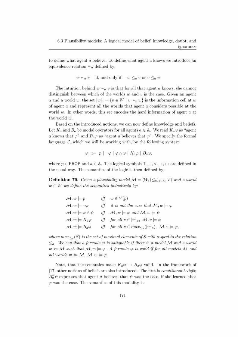
6.3 Plausibility models: A logical model of belief, knowledge, doubt, andignorance

to define what agent a believe. To define what agent a knows we introduce an

equivalence relation ∼a defined by:

w ∼a v if, and only if w ≤a v or v ≤a w

The intuition behind w ∼a v is that for all that agent a knows, she cannot

distinguish between which of the worlds w and v is the case. Given an agent

a and a world w, the set |w|a = {v ∈W | v ∼a w} is the information cell at w

of agent a and represent all the worlds that agent a considers possible at the

world w. In other words, this set encodes the hard information of agent a at

the world w.

Based on the introduced notions, we can now define knowledge and beliefs.

LetKa and Ba be modal operators for all agents a ∈ A. We readKaϕ as “agent

a knows that ϕ” and Baϕ as “agent a believes that ϕ”. We specify the formal

language L, which we will be working with, by the following syntax:

ϕ ::= p | ¬ϕ | ϕ ∧ ϕ | Kaϕ | Baϕ,

where p ∈ PROP and a ∈ A. The logical symbols >,⊥,∨,→,↔ are defined in

the usual way. The semantics of the logic is then defined by:

Definition 79. Given a plausibility model M = 〈W, (≤a)a∈A, V 〉 and a world

w ∈W we define the semantics inductively by:

M, w |= p iff w ∈ V (p)

M, w |= ¬ϕ iff it is not the case that M, w |= ϕ

M, w |= ϕ ∧ ψ iff M, w |= ϕ and M, w |= ψ

M, w |= Kaϕ iff for all v ∈ |w|a, M, v |= ϕ

M, w |= Baϕ iff for all v ∈ max≤a(|w|a), M, v |= ϕ,

where max≤a(S) is the set of maximal elements of S with respect to the relation

≤a. We say that a formula ϕ is satisfiable if there is a model M and a world

w in M such that M, w |= ϕ. A formula ϕ is valid if for all models M and

all worlds w in M, M, w |= ϕ.

Note, that the semantics make Kaϕ → Baϕ valid. In the framework of

[17] other notions of beliefs are also introduced. The first is conditional beliefs;

Bϕaψ expresses that agent a believes that ψ was the case, if she learned that

ϕ was the case. The semantics of this modality is:

171

Ch. 6. A Logic-Based Approach to Pluralistic Ignorance

M, w |= Bϕaψ iff for all v ∈ max≤a(|w|a ∩ [[ϕ]]M), M, v |= ψ,

where [[ϕ]]M is the set of worlds in M where ϕ is true. Another notion of

belief is safe belief for which we use �a. The semantics of this modality is:

M, w |= �aϕ iff for all v ∈W, if w ≤a v, then M, v |= ϕ.

Note, this is the usual modality defined from the relation ≤a. Since ≤a is

reflexive, �aϕ → ϕ is valid. Hence, safe belief is a very strong notion of

belief (or a weak notion of knowledge). Because a central aspect of pluralistic

ignorance is people holding wrong beliefs, safe belief is not a suitable notion.

Yet another notion of belief, that also implies truth, is weakly safe belief �weaka

given by the following semantics:

M, w |= �weaka ϕ iff M, w |= ϕ and for all v ∈W, if w <a v, then M, v |= ϕ,

where <a is defined by; w <a v if and only if w ≤a v and v 6≤a w. Finally, [17]

define strong belief Sba by

Sbaϕ iff Baϕ ∧Ka(ϕ→ �aϕ).

In addition to the several notions of belief, [17] also discuss several ways

of updating knowledge and beliefs when new information comes about. These

are update, radical upgrade, and conservative upgrade and can be distinguished

by the trust that is put in the source of the new information. If the source is

known to be infallible, it should be an update. If the source is highly reliable,

it should be a radical upgrade and if the source is just barely trusted, it should

be a conservative upgrade. In this paper we are interested in what it takes

to dissolve pluralistic ignorance and since update is the “strongest” way of

updating knowledge and beliefs, we will focus on this. We will also refer to

this way of updating as public announcement.

We introduce operators [!ϕ], and add to the syntax the clause that for

all formulas ϕ and ψ, [!ϕ]ψ is also a formula. [!ϕ]ψ is read as “after an

announcement of ϕ, ψ is true”. Semantically, a public announcement of ϕ will

result in a new plausibility model where all the ¬ϕ-worlds have been removed,

and the truth of ψ is then checked in this new model. These intuitions are

made formal in the following definition:

172

6.4 Modeling pluralistic ignorance

Definition 80. Given a plausibility model M = 〈W, (≤a)a∈A, V 〉 and a for-

mula ϕ, we define a new model M!ϕ = 〈W ′, (≤′a)a∈A, V ′〉 by,

W ′ = {w ∈W | M, w |= ϕ}≤′a = ≤a ∩(W ′ ×W ′)

V ′(p) = V (p) ∩W ′

The semantics of the public announcement formulas are then given by:

M, w |= [!ϕ]ψ iff if M, w |= ϕ then M!ϕ, w |= ψ.

Finally, we add to the framework of [17] the two notions of ignorance

and doubt. These are notions rarely discussed in the literature on epis-

temic/doxastic logic. However, ignorance is discussed in [159]. On the syn-

tactic level we add two new operators Ia and Da for each agent a ∈ A. The

formula Iaϕ is read as “agent a is ignorant about ϕ” and Daϕ is read as “agent

a doubts whether ϕ”. The semantics of these operators are defined from the

semantics of the knowledge operator and the belief operator:

Definition 81. The operators Ia and Da are defined by the following equiva-

lences:

Iaϕ := ¬Kaϕ ∧ ¬Ka¬ϕDaϕ := ¬Baϕ ∧ ¬Ba¬ϕ.

Note that, since Kaϕ→ Baϕ is valid, Daϕ→ Iaϕ is also valid.

6.4 Modeling pluralistic ignorance

Based on the logic introduced in the previous section, we will now formalize

different versions of pluralistic ignorance that are all consistent. Then, we will

discuss whether these formalizations make pluralistic ignorance into a fragile

phenomenon.

6.4.1 Formalizations and consistency of pluralistic ignorance

As discussed in Section 6.2, there are many ways of defining pluralistic igno-

rance and in this section we attempt to formalize a few of these. We will also

discuss whether these formalizations lead to consistent concepts in the sense

that the formalizations are satisfiable formulas.

173

Ch. 6. A Logic-Based Approach to Pluralistic Ignorance

Figure 6.1: A plausibility model where (6.1) is satisfiable at the root.

Firstly, we assume that pluralistic ignorance is a situation where no agent

believes ϕ, but every agent believes that everyone else believes ϕ. This can

easily be formalized as: ∧a∈A

(¬Baϕ ∧

∧b∈A\{a}

BaBbϕ)

(6.1)

For boolean formulas ϕ3, (6.1) is satisfiable since a plausibility model can

easily be constructed such that it contains a possible world that satisfies it.

Such a model is given in Figure 6.1, where we assume that the set of agents

is A = {a1, a2, ..., an}. In the following, when drawing models like this one,

an arrow from a state w to a state v labeled by ai will represent that w <ai v

holds in the model. An arrow from w to v labeled by a set B ⊆ A represent

that w <b v for all b ∈ B. The full plausibility relations of the model will be

the reflexive transitive closures of the relations drawn in the pictures. When

a formula ϕ appears next to a state it means that ϕ is true at that state.

There are also formulas ϕ for which (6.1) is unsatisfiable, take for instance

ϕ to be Bbψ or ¬Bbψ for any agent b ∈ A and any formula ψ. It cannot

be the case that agent a does not believe that agent b believes that ψ, but

at the same time a believes that b believes that b believes that ψ, i.e. (6.1)

is unsatisfiable when ϕ is Bbψ or ¬Bbψ because ¬BaBbψ ∧ BaBbBbψ and

¬Ba¬Bbψ ∧ BaBb¬Bbψ are unsatisfiable. In the following, when discussing

pluralistic ignorance as defined by (6.1) we will therefore assume that ϕ is a

boolean formula.

If belief is replaced by strong belief, such that (6.1) becomes∧a∈A

(¬Sbaϕ ∧

∧b∈A\{a}

SbaSbbϕ), (6.2)

3A formula is boolean if it constructed solely from propositional variables and the logical

connectives ¬, ∧, ∨, →, and ↔.

174

6.4 Modeling pluralistic ignorance

Figure 6.2: A plausibility model where (6.3) and (6.4) are satisfiable at the root.

pluralistic ignorance remains satisfiable for boolean formulas, which is testified

by Figure 6.1 again. Furthermore, (6.2) is also not satisfiable if ϕ is of the form

Sbbψ or ¬Sbbψ for a b ∈ A. However, if we use safe belief and weak safe belief

instead of belief in (6.1), pluralistic ignorance becomes unsatisfiable. This is

obvious since both safe belief and weak safe belief implies truth.

In the classroom example of Section 6.2, a better definition of pluralistic

ignorance may be obtained using the ignorance operator. This leads to the

following definition of pluralistic ignorance:∧a∈A

(Iaϕ ∧

∧b∈A\{a}

Ba¬Ibϕ)

(6.3)

This formula expresses a case where all the agents are ignorant about ϕ,

but believe that all the other agents are not ignorant about ϕ. Instead of

ignorance, doubt could be used as well, providing yet another definition of

pluralistic ignorance: ∧a∈A

(Daϕ ∧

∧b∈A\{a}

Ba¬Dbϕ)

(6.4)

Note that, since Daϕ→ Iaϕ, (6.4) implies (6.3).

The two definitions of pluralistic ignorance (6.3) and (6.4) are also eas-

ily seen to be satisfiable for boolean formulas ϕ. This is made apparent by

Figure 6.2. Now, however, formulas of the form Bbϕ, for b ∈ A, can also be

subject to pluralistic ignorance. It is possible that agent a can doubt whether

agent b believes ϕ and at the same time believe that agent b does not doubt

whether he himself /agent b believes ϕ.

In (6.3) and (6.4) we can also replace the belief operator by the strong

belief operator and obtain the following versions of pluralistic ignorance:∧a∈A

(Iaϕ ∧

∧b∈A\{a}

Sba¬Ibϕ)

(6.5)

175

Ch. 6. A Logic-Based Approach to Pluralistic Ignorance

∧a∈A

(Daϕ ∧

∧b∈A\{a}

Sba¬Dbϕ)

(6.6)

These new definitions of pluralistic ignorance are consistent as they are

satisfied at the root of the model in Figure 6.2. We still cannot obtain versions

of (6.3) and (6.4) with safe belief and weak safe belief for the same reason as

before.

It seems obvious that we can formalize even further versions of plural-

istic ignorance within this framework. Thus, using the logic introduced in

Section 6.3, we can characterize and distinguish many different versions of

pluralistic ignorance. Furthermore, all the definitions (6.1)-(6.6) were satis-

fiable, which seems to entail that the concept of pluralistic ignorance is not

inconsistent.

6.4.2 The fragility of pluralistic ignorance

After having formalized different versions of pluralistic ignorance, we can ask

whether any of the definitions entail that pluralistic ignorance is a fragile

phenomenon. However, first of all we need to spell out what we mean by a

fragile phenomenon. The question of whether pluralistic ignorance is fragile

or not reduces to the question of what it takes to dissolve it. We will regard

pluralistic ignorance as dissolved only when none of the agents have wrong

beliefs about the other agents’ beliefs anymore. The way agents can change

their beliefs, will in this section be modeled by the [!ϕ] operators of Section 6.3.

For the time being, we fix pluralistic ignorance to be defined as (6.1).

According to several descriptions of pluralistic ignorance, it should be dis-

solved if just one agent announces his true beliefs. If the formula !¬Bbϕ is

announced, it naturally follows that∧a∈ABa¬Bbϕ. However, this does not

dissolve the pluralistic ignorance since all agents might keep their wrong be-

liefs about any other agent than b. In other words, a model satisfying (6.1)

can be constructed such that after the announcement of !¬Bbϕ it still holds

that∧a∈A

(∧c∈A\{a,b}BaBcϕ

).

It turns out that there is nothing in the definition (6.1) that prevents the

wrong beliefs of the agents from being quite robust. Even if everybody except

an agent c announces that they do not believe ϕ, all the agents might still

believe that c believes ϕ. Using a formula of L we can define a notion of

robustness in the following way: agent a robustly believes that the group of

agents B ⊆ A\{a} believes ϕ if

176

6.4 Modeling pluralistic ignorance

Figure 6.3: A robust model where agent 1 believes ¬ϕ and has a strong robust belief that

the agents 2, 3, 4, and 5 believe ϕ. The worlds marked with “◦” are worlds where ¬ϕ is

true and the “clouds” marked with ϕ are collections of worlds where ϕ is true all over. The

arrows not marked with numbers represnt the plausibility raltion for agent 1 only.

∧C⊆B

([!¬Bcϕ]c∈C

( ∧b∈B\C

BaBbϕ)), (6.7)

where [!¬Bcϕ]c∈C is an abbreviation for [!¬Bc1ϕ][!¬Bc2ϕ]...[!¬Bckϕ], when

C = {c1, c2, ..., ck}.4 An example of a model where agent 1 believes ¬ϕ and

robustly believes that the agents {2, 3, 4, 5} believe ϕ is shown in Figure 6.3.

4An alternative to (6.7) is∧C⊆B

([!∧c∈C

¬Bcϕ]( ∧b∈B\C

BaBbϕ)),

however, the two are not equivalent. We will not go into a discussion of which definition is

preferable.

177

Ch. 6. A Logic-Based Approach to Pluralistic Ignorance

If in the model of Figure 6.3 it is announced that ¬B2ϕ then all the ◦-worlds that have an outgoing arrow marked with 2 will be removed. Thus,

the new “top” ◦-world will be the ◦-world with an outgoing arrow marked

345, which means that agent 1 still believes that the agents 3, 4, and 5 believe

ϕ. Note that if it is announced that ¬B1ϕ, what happens depends on the

plausibility relation for agent 1 within the ϕ-clouds, and this plausibility rela-

tion is unspecified in the model of Figure 6.3. However, one could define the

plausibility relation of agent 1 within the ϕ-clouds such that nothing happens

to the model if ¬B1ϕ is announced.

Another way of looking at the formula (6.7) is that it describes a situ-

ation where agent a believes that all the other agents’ beliefs about ϕ are

independent; maybe they all believe ϕ for different reasons. Thus, learning

about some agents’ beliefs about ϕ tells a nothing about what the other agents

believe about ϕ.

With robustness defined by (6.7), pluralistic ignorance is consistent with all

the agents having wrong robust beliefs about the other agents’ beliefs. Taking

disjoint copies of the model in Figure 6.3 for each agent and joining the roots

shows that:

Proposition 82. Pluralistic ignorance in form of (6.1) is consistent with that

all the agents a ∈ A, robustly believes that the group of agents A\{a} believe

ϕ.

Another way of interpreting this result is that announcements of the true

beliefs of some of the involved agents are not enough to dissolve pluralistic

ignorance. Either all the agents need to announce their true beliefs or new

information has to come from an outside trusted source. Thus, announcements

of the forms !Baϕ or !¬Baϕ are not guaranteed to dissolve pluralistic ignorance.

However, a public announcement of !¬ϕ in the model of Figure 6.3 will remove

the pluralistic ignorance. But an announcement of the form !¬ϕ (or !ϕ) is

precisely an announcement from a trusted outsider. An agent a in A can only

announce formulas of the form !Baψ or !¬Baψ.

What turns pluralistic ignorance into a fragile phenomenon in most cases, is

the fact that the agents consider the other agents’ beliefs not to be independent

as is the case if (6.7) is satisfied. In other words, pluralistic ignorance in

the fragile form occurs mainly when the beliefs of the involved agents are

correlated. This fits well with the view that pluralistic ignorance is a genuine

social phenomenon as claimed by [122].

Proposition 82 only regards pluralistic ignorance as defined by (6.1). How-

178

6.4 Modeling pluralistic ignorance

Figure 6.4: A robust model where agent 1 doubts whether ϕ and has a strong robust

belief in that the agents 2, 3, 4, and 5 do not doubt whether ϕ. The worlds marked with

“◦” are worlds where ¬ϕ is true and the worlds marked with “•” are worlds where ϕ is true.

The arrows with no numbers on are arrows for agent 1. Remeber that the full plausibility

relations of the model are the reflexive transitive closures of the arrows in the pictures.

ever, for the definitions (6.3) and (6.4) similar results hold. Neither of the

definitions (6.3) and (6.4) entail that pluralistic ignorance is fragile to public

announcements of doubts ([!Dbϕ]) or ignorance ([!Ibϕ]). We can construct

a new model, similar to the one in Figure 6.3, in which an agent a doubts

whether ϕ but has a strong robust belief in that all the agents in A\{a} do

not doubt whether ϕ (and the same goes for ignorance). This new model is

shown in Figure 6.4.

When it comes to the definitions of pluralistic ignorance based on strong

beliefs (6.2), (6.5), and (6.6), something interesting happens. In the model of

Figure 6.3 agent 1 does not have a strong belief that the other agents have

strong beliefs in ϕ. For instance, there is a state where B1Sb5ϕ and Sb5ϕ

are true, but �1Sb5ϕ is not true. The same issue occurs in the model of

Figure 6.4. It is still unknown whether robust models can be constructed such

that they satisfy the strong belief versions of pluralistic ignorance as defined

by (6.2), (6.5), and (6.6). Thus, it is left for further research whether there are

strong belief versions of pluralistic ignorance that are not fragile. There are

also several other questions for further research, which we will turn to now.

179

Ch. 6. A Logic-Based Approach to Pluralistic Ignorance

6.5 Further research on logic and pluralistic igno-

rance

We have given several consistent formalizations of pluralistic ignorance, but

there still seems to be more possible variations to explore. Furthermore, we

have been working within one specific framework, and the question remains

whether there are other natural frameworks in which all formalizations of

pluralistic ignorance become inconsistent. This would be highly unexpected

though. Another question regarding formalizations of pluralistic ignorance in

different frameworks is whether it changes the fragility of the phenomenon.

This is still an open question.

Even though pluralistic ignorance need not be fragile, neither as a “real

life” phenomenon nor according to the formalizations given in this paper, it

seems that the really interesting cases occur when pluralistic ignorance is, in

fact, fragile. Whether pluralistic ignorance is fragile appears to be closely re-

lated to it being a genuine social phenomenon; the dependence between agents’

beliefs is what makes pluralistic ignorance fragile. Thus, the real interesting

question for further research is how agents’ beliefs are interdependent in the

case of pluralistic ignorance and how best to model this in logic. In answer-

ing this question, a shift in focus from what it takes to dissolve pluralistic

ignorance, to what it takes for pluralistic ignorance to arise, seems natural.

6.5.1 Informational Cascades: How pluralistic ignorance comes

about and how it vanishes

An agent’s beliefs may depend on other agents’ beliefs in many ways; one

way is through testimony of facts by other agents in which the agent trusts.

Modeling trust and testimony is for instance done in [99]. Another way in

which agents’ beliefs may depend on each other could be through a common

information source [23]. Yet another way is through informational cascades.

Informational cascades are phenomena widely discussed in the social sci-

ences [23, 112] and the therm was introduced by [22]. Assume that some agents

are supposed to act one at a time in a given order and that their actions de-

pend on a private information source as well as the information obtained by

observing the actions of the agents already having acted. When actions are

performed sequentially and agents start to ignore their private information and

instead base their actions merely on information obtained from the actions of

the previous agents, an informational cascade has occurred. If the actions of

180

6.5 Further research on logic and pluralistic ignorance

the first people in the cascade oppose to their private beliefs and the remaining

people join in with the same actions (also oppose to their private beliefs) the

result might be a case of pluralistic ignorance. However, informational cas-

cades are also fragile [22] and opposite cascades may occur, thus eliminating

pluralistic ignorance again.

These kinds of informational cascades, which have been shown to occur in

numerous of places, may very well be the cause of pluralistic ignorance. Hence,

logical frameworks that can model informational cascades might also be suited

to model pluralistic ignorance. To the knowledge of the author, the only paper

on logic-based models of informational cascades is [99] and it may very well be

possible to model pluralistic ignorance in that framework. However, further

work on the logics of informational cascades is still to come.

6.5.2 Private versus public beliefs – the need for new notions

of group beliefs

The concept of pluralistic ignorance, regardless of which version one adopts,

seems to hint at the need for new notions of common knowledge/beliefs. Plu-

ralistic ignorance can be viewed as a social phenomenon where everybody holds

a private belief in ϕ, but publicly display a belief in ¬ϕ and thus contribute

to a “common belief” (“public belief” might be a better world) in ¬ϕ. Due

to the usual definition of common belief (everybody believes ϕ and everybody

believes that everybody believes ϕ and ...), a common belief in ¬ϕ leads to

private belief in ¬ϕ for all agents in the group, but this is exactly the thing

that fails in social epistemic scenarios involving pluralistic ignorance. Hence,

a new notion of common group belief seems to be needed. In general, there

are various ways in which group beliefs can be related to the beliefs of individ-

uals of the group. Thus, a logic that distinguishes between private and public

beliefs or contains new notions of common beliefs may help model pluralistic

ignorance more adequately. Once again, this is left for further research.

6.5.3 How agents act

The way agents act in cases of pluralistic ignorance also seems to play an

important role. The reason why most students believe that other students

are comfortable with drinking might be that they observe the other students

drinking heavily. In the classroom example students are also obtaining their

wrong beliefs based on the observation of others. Furthermore, focusing on

181

Ch. 6. A Logic-Based Approach to Pluralistic Ignorance

actions might also tell us something about how pluralistic ignorance evolves

in the first place.

Therefore, a logic combining beliefs and actions might be the natural tool

for modeling pluralistic ignorance. There exist several logics that combine be-

liefs/knowledge and actions, but which one to chose and the actual modeling,

is left for further research to decide.

6.6 Conclusion

Firstly, we have seen that there are many ways of defining pluralistic igno-

rance, all of which by satisfiable formulas. Therefore, pluralistic ignorance is

(seemingly) not a phenomenon that goes against logic. In other words, wrong

logical reasoning is not necessarily involved in pluralistic ignorance.

Secondly, the standard definitions of pluralistic ignorance, for instance as

a situation where no one believes, but everyone believes that everyone else

believes, do not entail that the phenomenon is fragile. Public announcements

of the true beliefs of some of the involved agents are not enough to dissolve

pluralistic ignorance. Either all the agents need to announce their true beliefs

or new information has to come from an outside, trusted source. However,

pluralistic ignorance often seems to occur in cases where the agents’ beliefs

are correlated and in such cases pluralistic ignorance might be increasingly

more fragile.

The paper has hinted at a first logic approach to pluralistic ignorance.

Some features and problems have been singled out, but the main aim of the

paper was to pave the way for further research into logical modeling of social

phenomena such as pluralistic ignorance.

Acknowledgment

The author would like to thank Vincent Hendricks for suggesting the topic.

Furthermore, the author would like to thank the participants of the workshop

PhDs in Logic III (Brussels, February 17-18th, 2011) and the participants

of the Copenhagen-Lund workshop in Social Epistemology (Lund, February

25th, 2011). Finally, the author would like to thank Jens Christian Bjerring,

Nikolaj Jang Lee Linding Pedersen, Carlo Proietti, Vincent F. Hendricks, Eric

Pacuit, and Olivier Roy for useful discussions and comments.

182

Chapter 7

Logical Knowledge Representation of

Regulatory Relations in Biomedical

Pathways

(co-authored with Sine Zambach)

Published in Lecture Notes in Computer Science volume 6266: 186–

200, 2010. Proceedings of the 1st International Conference on Infor-

mation Technology in Bio- and Medical Informatics (ITBAM 2010).

Abstract: Knowledge on regulatory relations, in for example reg-

ulatory pathways in biology, is used widely in experiment design by

biomedical researchers and in systems biology. The knowledge has

typically either been represented through simple graphs or through

very expressive differential equation simulations of smaller sections

of a pathway.

As an alternative, in this work we suggest a knowledge represen-

tation of the most basic relations in regulatory processes regulates,

positively regulates and negatively regulates in logics based on a

semantic analysis. We discuss the usage of these relations in bi-

ology and in artificial intelligence for hypothesis development in

drug discovery.

Keywords: Formal relations, semantic analysis, biomedical on-

tologies, knowledge representation, knowledge discovery, applied

logic, formal ontologies.

183

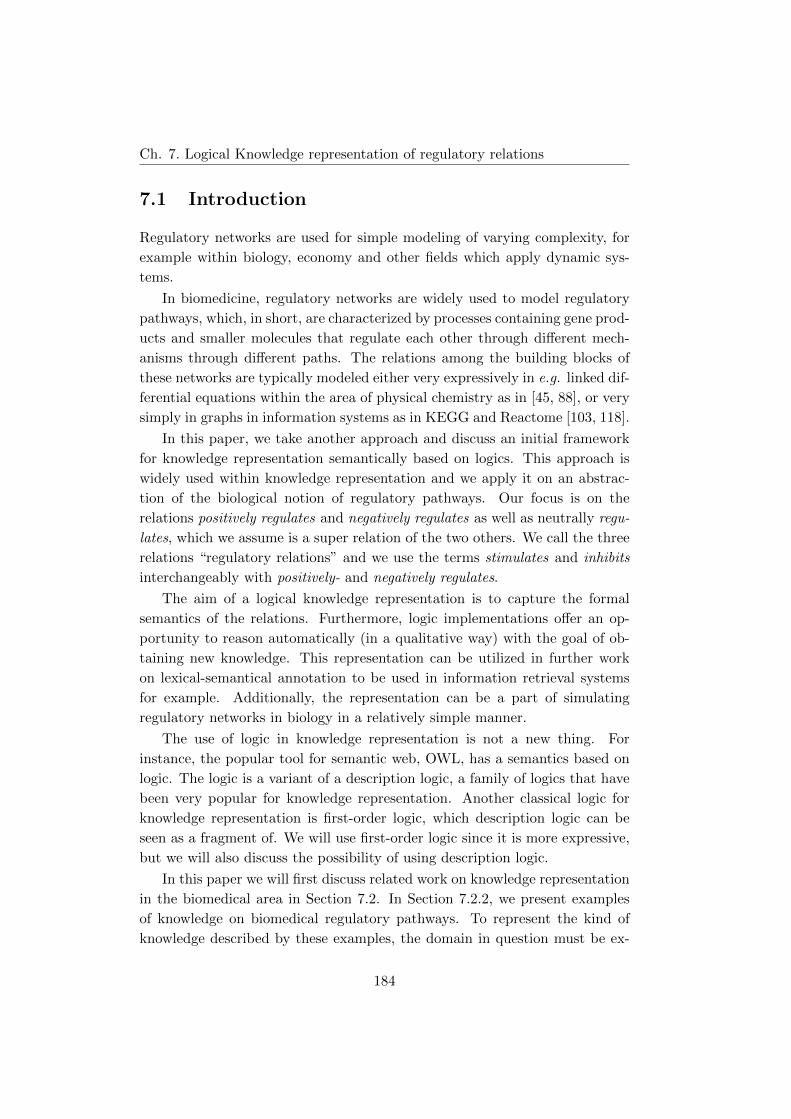
Ch. 7. Logical Knowledge representation of regulatory relations

7.1 Introduction

Regulatory networks are used for simple modeling of varying complexity, for

example within biology, economy and other fields which apply dynamic sys-

tems.

In biomedicine, regulatory networks are widely used to model regulatory

pathways, which, in short, are characterized by processes containing gene prod-

ucts and smaller molecules that regulate each other through different mech-

anisms through different paths. The relations among the building blocks of

these networks are typically modeled either very expressively in e.g. linked dif-

ferential equations within the area of physical chemistry as in [45, 88], or very

simply in graphs in information systems as in KEGG and Reactome [103, 118].

In this paper, we take another approach and discuss an initial framework

for knowledge representation semantically based on logics. This approach is

widely used within knowledge representation and we apply it on an abstrac-

tion of the biological notion of regulatory pathways. Our focus is on the

relations positively regulates and negatively regulates as well as neutrally regu-

lates, which we assume is a super relation of the two others. We call the three

relations “regulatory relations” and we use the terms stimulates and inhibits

interchangeably with positively- and negatively regulates.

The aim of a logical knowledge representation is to capture the formal

semantics of the relations. Furthermore, logic implementations offer an op-

portunity to reason automatically (in a qualitative way) with the goal of ob-

taining new knowledge. This representation can be utilized in further work

on lexical-semantical annotation to be used in information retrieval systems

for example. Additionally, the representation can be a part of simulating

regulatory networks in biology in a relatively simple manner.

The use of logic in knowledge representation is not a new thing. For

instance, the popular tool for semantic web, OWL, has a semantics based on

logic. The logic is a variant of a description logic, a family of logics that have

been very popular for knowledge representation. Another classical logic for

knowledge representation is first-order logic, which description logic can be

seen as a fragment of. We will use first-order logic since it is more expressive,

but we will also discuss the possibility of using description logic.

In this paper we will first discuss related work on knowledge representation

in the biomedical area in Section 7.2. In Section 7.2.2, we present examples

of knowledge on biomedical regulatory pathways. To represent the kind of

knowledge described by these examples, the domain in question must be ex-

184

7.2 Related work and examples

Figure 7.1: A chain of inhibitions and stimulations in the insulin signaling

pathway (simplified). The figure is a modified picture from KEGG [103].

posed to a deeper ontological investigation. Furthermore, the clarification of

the ontology displays which underlying assumptions are involved in the knowl-

edge we aim to represent. These issues will be discussed in Section 7.3. In

Section 7.4, we use First-order Logic to specify a formal semantics of regula-

tory relations. Next, we analyze the entities involved in regulatory relations,

which allows us to clarify regulatory relationships even further. In addition,

we discuss the possibilities of representing the relations in Description Logic.

Finally, we discuss the biological usage of our formalization of the regulatory

networks and further work.

7.2 Related work and examples

7.2.1 Related work

Knowledge representation of biomedical pathways typically spans from simple

graph representations among gene products to the more sophisticated linked

differential equations, as already mentioned.

Graph representations are mostly informal and constructed to illustrate a

regulatory path. In more formal graphs like KEGG [103] (in Figure 7.1), Re-

actome [118], and MetaCyc [45], regulation among entities like small molecules

and gene products are formalized into a database, to which you can have sim-

ple queries. For example, in the network of Figure 7.1, the legend tells us that

“PP1 activates GYS” (because of the arrow) and “PP1” is a gene product (be-

cause of the box around “PP1”), which is information stored in the relatively

simple structure of KEGG.

At the other end of the scale, regulatory pathways can be represented using

linked differential equations expressed in the formula:

185

Ch. 7. Logical Knowledge representation of regulatory relations

dSi/dt = fi(Sj , pk) = f+i + f−i

i,j=(1,...,n)k=(1,...,m) . (7.1)

For our purpose, the two most important parameters are f+i , the sum of

the incoming flux (leading to positive regulation), and f−i , the sum of the

outgoing flux leading to negative regulation [88]. This representation is very

expressive and will be difficult if not impossible to implement on the almost

10,000 reactions that are represented in KEGG [45].

Additionally, the problems of acquiring such detailed information and the

computationally higher complexity in these models, have lead to suggest less

complex models, as for instance in [55]. This simpler model makes it possible

to reason qualitatively about existing pathways leading to a rough flux-balance

analysis similar to MetaCyc [45] and BioSim [87], which uses Prolog and qual-

itative constraints.

During the last decade a movement towards formalizing biomedical on-

tologies and the relations the ontologies contain, has progressed. For example,

the widely used Gene Ontology [123, 9] has been ontologically “cleaned up”

and initiatives like OBO have provided a framework for the work on formal

relations and cooperative ontology modeling [139, 32]. Moreover, concern-

ing properties of relations, the Role Ontology has been developed within the

OBO foundry [140]. In the pathway modeling, especially concerning regula-

tion, ontologies and formalized systems like the Gene Regulation Ontology

[20], EcoCyc/MetaCyc [45] and Pathway Logics [55] have suggested different

approaches to logic representation. Furthermore, in the work on the Gene

Regulation Ontology(GRO), regulation is present as a concept. The purpose

of that work is to formalize the concepts related to gene regulation used in for

example the Gene Ontology [9].

This work introduces First-order Logic in the representation in line with

[140], for example.

7.2.2 Examples of regulation

To be able to argue for the ontological assumptions in Section 7.3 and the logi-

cal semantic presented in Section 7.4, in this section, we will present examples

of the knowledge our simple model is supposed to capture.

The regulates-relations positively regulates and negatively regulates - are

central in for example economics and biochemical pathways. In biomedical

pathways, which we will concentrate on in the rest of this paper, it is typical

186

7.3 Ontological clarifications

gene products and smaller molecules that interact with each other in complex

processes.

A commonly used example of regulation is the insulin response mecha-

nism. Insulin stimulates through a regulatory path, uptake of glucose through

cell walls, protein synthesis and glucogenesis, for example. These stimulations

occur via for example an activation of PIP3 and the glucogenesis is triggered

for example through an activation of the Akt-protein and inhibition of PHK

as shown in Figure 7.1. Note here, that most of the regulatory paths are

between the biological entities, gene products and small molecules. This typ-

ically means that one biological entity regulates the level (by regulating the

production/secretion process) or function of another biological entity.

Another example of how regulation in a biological pathway has been rep-

resented semi-formally for use in hypothesis testing, is the presentation of the

damage response pathway in yeast, which has been investigated and charac-

terized by for example [173]. This work is a usage of a strategy for a longer

pathway-traveling concerning gene products that regulate the production of

other gene products. The work uses the notion of “deletion-buffering”. The

meaning of this is: When you remove a transcription factor, X, of the gene

product, G, the result is that the production of another protein, P, cannot be

regulated anymore by G, if G interacts directly with P. This typically results

in an activation of P if G is an inhibitor and an inhibition of P if G is an

activator.

There will of course be examples that are non-trivial compared to the

above mentioned examples. An example is predicted inhibition in the recently

discovered miRNAs, which are small regulating transcripts. miRNAs typically

regulate gene products by binding to the mRNA of the gene product. However,

often the regulation is just predicted in silico by sequence analysis until the

experimental data has verified (or falsified) the interaction. This information

is difficult to model by a simple regulates-relations since the meaning is rather

“predicted to inhibit”. We will return to this issue in Section 7.4.3.

7.3 Ontological clarifications

Based on the previous presented examples, we investigate in more detail

the ontological aspects of regulatory relations as they present themselves in

biomedical research. We clarify which entities are subject to relationships

and make a distinction between general concepts or classes and individuals

instantiating these classes.

187

Ch. 7. Logical Knowledge representation of regulatory relations

7.3.1 Research practice and granularity

When creating models of knowledge to be used in biomedical hypothesis de-

velopment, inspiration can be obtained by the practice in the biomedical lab-

oratory. Before the validation of a hypothesis is to be carried out in the

laboratory, the precise rates and levels of the involved substances are not nec-

essarily the first thing to consider. Rather we consider a qualitative overview

of the processes to be the primary instrument in this stage of discovery. Thus

we ignore the precise levels of substances and only care whether their levels are

affected positively or negatively, leaving us with a higher level of abstraction

(as in [55]).

Likewise, talking about “insulin positively regulates glucose transport”,

what is really meant is that an amount (or pool) of insulin causes an amount

of glucose molecules to be transported. Or, expressed more precisely: When

the level of insulin rises, this rise causes a higher frequency of glucose molecules

to be transported (through cell walls). This rise is typically directly or indi-

rectly caused by external addition of substance - either by intake of nutrition,

medication or even by lack of intake of the necessary nutrition to make the

system work properly. Hence “amounts” or “pools” of substances are the basic

entities, which are subject to possible relations.

7.3.2 Underlying ontological assumptions - Instances and classes

The former subsection suggests that amounts of molecules rather than single

molecules are the central concern of biomedical researchers. In laboratory con-

text, researchers operate with certain amounts or batches of fluids containing

multiple molecules. Also, the organs of the human body secrete an amount

of molecules for regulating processes. Nothing really happens if the beta cell

secretes one insulin molecule.

The ontological assumptions we make are virtually in line with the one

presented in [140] and [141]. As in [140], we will distinguish between classes

and instances. Classes (or concepts or types) refers here to what generally

exists, such as insulin, glucose, glucose transport, stem cell, etc.. In the fol-

lowing, names of classes will be italicized and begin with a capital letter, for

instance Insulin and Glucose transport. On the other hand, instances (or

individuals, particulars, or tokens) are entities that exist in space and time as

instances of a class, such as a particular quantity of insulin or beta cells. We

will use x, y, z, ... as variables ranging over arbitrary instances.

The distinction between classes and instances allows us to analyze a natural

188

7.4 Analysis of the formal semantic

language expression such as “insulin positively regulates glucose transport” in

more details; the sentence does not claim that the class Insulin positively regu-

lates the classGlucose transport, but that a certain relation between individu-

als of these classes exists as presented in Section 7.3.1. Thus we assume that re-

lations between the instances are given, for example by experimental evidence

in the laboratory, and on the basis of these we define relations among classes or

concepts. For instance, “positive regulation” relations may exists among par-

ticular amounts of insulin and particular glucose transports, and on the basis of

these we define a relation between the classes Insulin and Glucose transport.

This we will do in the next section. Names of relations among individuals will

be in bold face, e.g. “x stimulates y”, whereas names of relations among

classes will be in italic, e.g. “Insulin stimulates Glucose transport”.

7.4 Analysis of the formal semantic

In this section we provide a thorough semantic analysis of the regulatory rela-

tions based on First-order Logic. Finally, we mention the possibilities for an

analysis in Description Logic and OWL.

7.4.1 A Logic formalization of regulatory relations

Given the ontological assumptions, we will now discuss the possible relations

between classes involved in the knowledge we aim to represent. In the defini-

tion of relations among these classes we will use First-order Logic. First-order

Logic is used to reason about individuals and their properties, and allows for

quantification over these individuals. The language of First-order Logic is built

from propositional connectives such as “and” (∧), “or” (∨), “not” (¬), predi-

cate symbols involved in P (x) or Q(x, y), variables x, y, z, . . ., and quantifiers

∀ and ∃ (reading “for all” and “there exists”). We have chosen First-order

Logic because of its simple reading and generality.1

A first example of a formalized relation between classes is the “part of” re-

lation present in many biological ontologies. One can state that Cell membrane

is “part of” Cell, which expresses the fact that every particular cell membrane

is the membrane of a particular cell. In other words, “for every cell membrane

there exists a cell of which it is part of”. Assuming a part of relation between

1A commonly used logic for knowledge representation such as Description Logic can be

viewed as a fragment of First-order Logic. We will return to the possibilities of giving the

semantic in terms of Description Logic later in Section 7.4.4.

189

Ch. 7. Logical Knowledge representation of regulatory relations

individuals, one can define a part of relations among classes C1 and C2 in the

following way [141]:

C1 part of C2 iff ∀x(C1(x)→ ∃y(x part of y ∧ C2(y))). (7.2)

A relation between classes defined this way will for easy reading be called

“∀∃”. Generally we define a ∀∃ relation rel∀∃ between two classes, C1 and C2,

based on a relation rel between individuals, by:

C1 rel∀∃ C2 iff ∀x(C1(x)→ ∃y(x rel y ∧ C2(y))). (7.3)

The two classes C1 and C2 are also called the relata of the relation. Another

example of a concrete relation between classes is the one exemplified by the

term “enzymes stimulate processes”. Even though it may not be visible on

the surface, what we have here is an even stronger tie between the two classes

than expressed by a ∀∃ relation. The relation between enzymes and process

is such that whatever an enzyme stimulates, it is a process. A relation of this

kind will be called “∀only”. Formally we define the ∀only relation by:

C1 rel∀only C2 iff ∀x(C1(x)→ ∀y(x rel y → C2(y))). (7.4)

We now consider the case positively regulates as exemplified by a phrase

such as “insulin positively regulates glucose transport”, which exemplifies

the kind of knowledge we aim to represent. As previously discussed in Sec-

tion 7.3.1, a sentence like this should be read as “for all amounts of insulin and

all glucose transports, the insulin can potentially positively regulate the glu-

cose transport”. To express a relation like this we introduce the “∀∀” relation

between classes in the following way:

C1 rel∀∀ C2 iff ∀x(C1(x)→ ∀y(C2(y)→ x rel y)). (7.5)

The reason for choosing the ∀∀ relation instead of the ∀only to represent

knowledge such as “insulin positively regulates glucose transport”, is that

Insulin also has the possibility to stimulate other processes such as glycogen

production. This possibility is excluded if the knowledge is represented as a

∀only relation.

7.4.2 The relata of regulatory relations

A deeper ontological analysis of the entities involved in regulatory relations

reveals that a distinction between continuants and processes has ontological

190

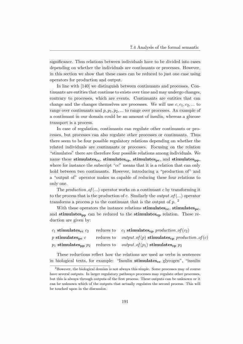
7.4 Analysis of the formal semantic

significance. Thus relations between individuals have to be divided into cases

depending on whether the individuals are continuants or processes. However,

in this section we show that these cases can be reduced to just one case using

operators for production and output.

In line with [140] we distinguish between continuants and processes. Con-

tinuants are entities that continue to exists over time and may undergo changes,

contrary to processes, which are events. Continuants are entities that can

change and the changes themselves are processes. We will use c, c1, c2, ... to

range over continuants and p, p1, p2, ... to range over processes. An example of

a continuant in our domain could be an amount of insulin, whereas a glucose

transport is a process.

In case of regulation, continuants can regulate other continuants or pro-

cesses, but processes can also regulate other processes or continuants. Thus

there seem to be four possible regulatory relations depending on whether the

related individuals are continuants or processes. Focusing on the relation

“stimulates” there are therefore four possible relations among individuals. We

name these stimulatescc, stimulatescp, stimulatespc, and stimulatespp,

where for instance the subscript “cc” means that it is a relation that can only

hold between two continuants. However, introducing a “production of” and

a “output of” operator makes us capable of reducing these four relations to

only one.

The production of (...) operator works on a continuant c by transforming it

to the process that is the production of c. Similarly the output of (...) operator

transforms a process p to the continuant that is the output of p. 2

With these operators the instance relations stimulatescc, stimulatespc,

and stimulatespp can be reduced to the stimulatescp relation. These re-

duction are given by:

c1 stimulatescc c2 reduces to c1 stimulatescp production of (c2)

p stimulatespc c reduces to output of (p) stimulatescp production of (c)

p1 stimulatespp p2 reduces to output of (p1) stimulatescp p2

These reductions reflect how the relations are used as verbs in sentences

in biological texts, for example: “Insulin stimulatescc glycogen”, “insulin

2However, the biological domian is not always this simple. Some processes may of course

have several outputs. In larger regulatory pathways processes may regulate other processes,

but this is always through outputs of the first process. These outputs can be unknown or it

can be unknown which of the outputs that actually regulates the second process. This will

be touched upon in the discussion.

191

Ch. 7. Logical Knowledge representation of regulatory relations

stimulatescp the glycogenesis”, and “insulin stimulatescp the production of

glycogen (through the glygonenesis)” where the process glycogenese is equal to

“the production of glycogen”. Likewise you can formulate the sentences: “beta

cell secretion stimulatespp glycogenese” that can be reduced to “output of

beta cell secretion stimulatescp production of glycogen”, where the output

of beta cell secretion is insulin.

7.4.3 Modal, temporal and spatial aspect of regulatory rela-

tions

In the reading of “Insulin stimulates glucose transport” as “for all amounts

of insulin and all glucose transports, the insulin can potentially positively

regulate the glucose transport” the term “can potentially” plays a considerable

role. It is a vague modal term, and in this section we will attempt to make it

more precise.

When representing “Insulin stimulates glucose transport” as

∀x(Insulin(x)→ ∀y(Glucose transport(y)→ x stimulatescp y)),

the term “can potentially” is implicit in the relation “stimulatescp”. In

other words “x stimulatescp y” is read as “x can potentially stimulate y”.

This seems sensible since “Insulin stimulates glucose transport” does not ex-

press that all amounts of insulin actually stimulates all glucose transports, but

that they potentially can. Using modal logic formalisms [31] we can replace

“x stimulatescp y” by “♦(x stim y)”, where the “♦” is a modal operator

representing “potentiality” and “stim ” is the primitive name of a relation

of actual stimulation. Thus “c stim p” means that the continuant c actively

stimulating the process p. A semantics for this elaborated formula can then

be given in the framework of first-order modal logic [40].

The potentiality represented by the ♦ operator can, however, be ana-

lyzed even further in the case of the stimulation relation. There are two

kinds of vagueness involved in the “can potentially stimulate” expressed in

“♦(...stim...)”. The first one is due the fact that stimulation only takes place

if the substance is actively participating in the process. If the process and

substance are separated in space and time, stimulation can of course not take

place. The relation of a continuant taking actively part in a process at a given

time, is a basic relation and in [140] it is assumed as a primitive relation.

Using their notation “p has agent c at t” expresses that the continuant c is

causally active in the process p at time t. Together with the stim relation,

192

7.4 Analysis of the formal semantic

“c stimulatescp p” can thus be expanded as:

∀t(p has agent c at t→ c stim p),

hence the ♦ operator is unnecessary.

The other vagueness involved in “can potentially stimulate” is due to the

fact that other substances may interfere with the process, in which case a

stimulation may not take place. Thus, in the above formula, x stim y should

be read as “if no other substances interfere an actual stimulation between x

and y takes place”. If we use the formalization with the Diamond operator,

we can include this ceteris paribus clause in the reading of the ♦.

In non-trivial examples as the predicted regulation by miRNAs as described

in Section 7.2.2 there is an additional vagueness. This is due to the stimu-

lation only being predicted. For example, miRNA stimulatescc c (predicted

in silico), and c stimulatescp p should lead to a weaker inference between

miRNA and p than if the miRNA was experimentally shown to stimulate c.

7.4.4 Description Logic representation of class relations

In Section 7.4.1 we used First-order Logic to present a formal semantics for

regulatory relations. This was motivated by the easy reading of First-order

formulas that also made the difference between the class relations rel∀only and

rel∀∀ visible. In this section we discuss the possibility of defining the relations

in Description Logic.

Description Logic is a family of logics widely used for knowledge represen-

tation, and in several of the logics reasoning can be done in low complexity

contrary to First-order Logic which is undecidable (for more on the complexity

of Description Logic see chapter 3 in [12]). Furthermore, Description Logic is

also implemented in several modern tools such as OWL [76]. Proteg-OWL is

a popular language for knowledge representation and it can implement most

flavours of Description Logics although the OWL-full version of OWL.1 is

undecidable.

The two class relations rel∀∃ and rel∀only(defined in (7.3) and (7.4)) can

easily be formalized in Description Logic by:

C1 rel∀∃ C2 iff C1 v ∃rel.C2,

C1 rel∀only C2 iff C1 v ∀rel.C2.

However, the class relation rel∀∀ is not expressible in a majority of De-

scription Logics. Although in very expressible Description Logics including

193

Ch. 7. Logical Knowledge representation of regulatory relations

full concept negation and role negation [116, 114], the rel∀∀ relation can be

formalized by:

C1 rel∀∀ C2 iff C1 v ∀(¬rel).¬C2.

Alternatively a new operator in line with the “∃rel” and “∀rel” operators

could be added to a Description Logic. Such an operator has already been

added to similar modal logics and goes under the name “the window operator”.

However, a minimal Description Logic with this operator appears not to have

been investigated. Thus, there is still work left to be done in the field of

Description Logic before knowledge on regulatory relations can be optimally

represented.

7.5 Discussion

Based on an analysis of the biomedical examples and our declaration of the

ontological assumption, we have suggested that the correct formalizations of

positively and negatively regulates in First-order Logic are represented by the

formula ∀x(C1(x) → ∀y(C2(y) → x rel y)). A description of the relata,

the First-order formulas, and examples of regulates, positively regulates and

negatively regulates are displayed in Table 7.1.

Thus, our contribution to the field of knowledge representation and biomed-

ical informatics is a logical analysis and representation of regulatory relations.

One of the main advantages of modeling knowledge in a formal framework as

logic is that it makes entire knowledge bases available for consistency checks

and allows for the use of reasoning tools to gain new knowledge. This is par-

ticularly useful in for instance artificial intelligence and information retrieval.

In relation to the related work of Section 7.2, this formalization is in the

middle of a complexity scale. It is not as expressive as the linked differential

equations [88], but much better suited for automatic reasoning than simple

graphs [103]. In expressivity and tractability it is close to work like [55, 45].

However, this work provide a semantic and uses First-order Logic formaliza-

tion, which provides more information to the relations than the before men-

tioned due to the quantifications.

7.5.1 Applications in the biomedical domain

From a biological point of view, the main purpose of our formalization of the

regulatory relations is to assist knowledge discovery, hypothesis development,

194

7.5 Discussion

Table 7.1: Definitions of three regulatory relations. They are expressed as

class-level relations in a format similar to that of OBO Relation Ontology

[140]. Relation and relata capture the representation in e.g. KEGG, Defini-

tions displays the First-order Logic formalizations, and Examples contributes

with examples taken from pubmed-abstracts [132].

A. Regulates

Relations and relata C1 regulates∀∀ production of (C2); C1 and C2 are

continuants.

Definitions ∀x(C1(x)→ ∀y(production of (C2(y))→x regulates y)).

Examples

...nitric oxide pathway regulates pulmonary vascular tone...

...non-histone chromosomal proteins may modify gene

expression ...

...creb regulates cyclic amp-dependent gene...

B. Positively Regulates

Relations and relata C1 positively regulates∀∀ production of (C2); C1 and C2

are continuants.

Definitions ∀x(C1(x)→ ∀y(production of (C2(y))→x positively regulates y)).

Examples

...ipa stimulates insulin release...

...Ca(2+) influx stimulates exocytosis of secretory granules...

...mmp-7 activates the epidermal growth factor...

C. Negatively Regulates

Relations and relata C1 negatively regulates∀∀ production of (C2); C1 and

C2 are continuants.

Definitions ∀x(C1(x)→ ∀y(production of (C2(y))→x negatively regulates y)).

Examples

...glp-1inhibits glucagon release...

...lithium inhibits the enzyme glycogen synthase kinase-3...

...rsbx negatively regulates an extension of the rsbv-rsbw

pathway...

...insulin secretion from the β-cell to reduce iri responses...

195

Ch. 7. Logical Knowledge representation of regulatory relations

and, in a broader perspective, lexical resource integration of the semantics of

the words representing the relations.

7.5.1.1 Inferences and reasoning rules.

Proposing rules for reasoning in a logical framework allows us to obtain new

knowledge from an existing knowledge base.

First, we have the inferences that are given from the semantics of the First-

order Logic. For the relation regulates defined as in equation (7.5) we will

have the following inferences:

is a ◦ regulates→ regulates

regulates ◦ is a−1 → regulates

The ◦-operator is a common notation for composition of relation and the

is a relation is interpreted as the subset relation.

Additionally, you can create domain- or application-specific reasoning rules

depending on the amount of knowledge you want from your system. In imple-

menting artificial intelligent systems in biomedical informatics several reason-

ing rules have been suggested [175, 123].

A list of proposed rules can be found in [175]3 and in [123], and an example

of one of these is:

negatively regulates ◦ negatively regulates→ positively regulates

From the reasoning rules we can deduce additional relationships from ex-

isting ones, and we can make inferences such as: “if insulin stimulates glucose

transport and if the glucose transport inhibits glyconeogenesis, then insulin

inhibits glyconeogenesis”. Thus, if you want to find novel gene products and

molecules that regulate a given process or a given molecule in a certain way,

you can use reasoning rules to predict such. Another perspective of this auto-

mated reasoning is the prediction of the side effects of a drug or extra molecule

functions.

Furthermore, you can potentially place a new unfamiliar molecule correctly

in a regulatory pathway due to its regulatory properties. These functions can

be an advantage in drug discovery, identification of adverse effects and in

knowledge expansion for more fundamental research purposes. These are just

3The rules of [175] are meant to hold throughout the biomedical domain, however they

may not always reflect reality. Instead, they shoulde be viewed as rules of thumb, used to

infer possible new knowledge in drug discovery and hypothesis development.

196

7.5 Discussion

some of the many advantages a logic based knowledge representation, as the

one presented here, provides when fully implemented.

7.5.1.2 Towards implementation of a prototype.

The most straightforward evaluation would obviously be an implementation of

a prototype system for information retrieval and/or for hypothesis generation

that would use the suggested formalisation. A comparison with similar systems

not using the same formal representation of regulatory relations, would then

make the contribution of the semantical representation clear.

To illustrate the effects and properties of the relations we have constructed

a small example in the logical programming language Prolog. We have im-

plemented a small part of the KEGG database from Figure 7.1 containing 21

classes and the relations: is a, stimulates and inhibits. Besides the relations

in the figure, a small taxonomy is created such that we are able to separate

continuants such as (small molecule and gene product) and processes in cor-

respondence to the way KEGG names the entities.

The toy-implementation can be used to infer fundamental inheritances

in taxonomies of classes (ontology consisting of pure ISA-relations) as men-

tioned in the former subsection and can be downloaded and tested from:

www.ruc.dk/sz/Regrel. Further work needs to be done to prove that the se-

mantics of the implemented relations are actually equal to the semantics we

have suggested in this paper.

Another possibility is to implement the system in DL using the suggestion

in Section 7.4.4. However, this will require both full role-negation and full

concept negation and the tractability of this is to be investigated further.

7.5.1.3 Ontological aspects of regulation.

In Section 7.4.2 we made a distinction between continuants and processes,

leading us to a characterization of 4 different basic relations among individ-

uals. For stimulation these where the relations stimulatescc, stimulatescp,

stimulatespc, and stimulatespp, which we further reduced to the single rela-

tion stimulatescp. However, one may argue that the relations stimulatespcand stimulatespp are not genuine relations in the first place. From a strict

ontological point of view processes never stimulate other processes or contin-

uants directly, but always through their outputs.

197

Ch. 7. Logical Knowledge representation of regulatory relations

An example of this is glycogenesis4. Glycogen is an output of this pro-

cess, but other outputs occur as well, for example uridine diphosphate (UDP),

whose effects might be different that glycogen. Thus, when we have a state-

ment that the glycogenesis stimulates glucose homeostasis, we cannot be cer-

tain whether glycogen or UDP or both are the actors unless this is stated

explicitly. Nevertheless it is either glycogen or UDP (or both) that stimulate

homeostasis, and not actually glycogenesis.

We recognize that it is a debatable issue whether processes can stimulate

other processes or continuants. There seems to be evidence, however, that

it is important to investigate the ontological aspects of stimulation further.

Whether stimulation is among continuants or processes seems to have conse-

quences for the inference of new knowledge, and thus the distinction should be

recognized. In simple knowledge representations by graphs like in the KEGG

database such observations are not accounted for. Such knowledge bases have

the potential to get this representation integrated automaticaly when a se-

mantics is agreed upon.

7.5.2 Future work

With our discussions and examples we have revealed that several occurrences

of regulatory relationships are characterised by vagueness or fuzziness. How-

ever, one could take it one step further by taking the characteristic fuzziness

seriously and apply fuzzy logics or other logics of uncertainty to model this

aspect of the regulatory relationships.

As mentioned in Section 7.4.4 the logical framework of Description Logic

is still not fully developed for representing the formal semantics of regulatory

relations as we defined them in this paper. This is also a direction of future

work that may tell us something about how efficient we can do automatic

reasoning about regulatory relations in practice. Furthermore it may also

reveal how the relations can be incorporated into for instance OWL.

Staying within the field of logic, we mentioned several possible class rela-

tions in Section 7.4.1 and a deeper analysis of all possible class relations and

there properties would also be interesting future work.

We finally suggest that the formal semantic analysis presented in Sec-

tion 7.4 can be used to define frame semantics for the verbs and verb phrases

that express regulatory relations. The definition of the frame semantics is sim-

4Note that glycogenesis and the above mentioned glyconeogenesis are two different pro-

cesses.

198

7.5 Discussion

ilar to the one we find in the work done in BioFrameNet [53] on other verbs.

The attempt of defining frame semantics may well result in an enrichment of

semantically annotated data and for instance be applied to semantic querying

[6].

Acknowledgment

We would like to thank Mai Ajspur for useful comments on and discussions

of an earlier version of this paper and Jørgen Fischer Nilsson for an insightful

discussion of the class relations.

199

Ch. 7. Logical Knowledge representation of regulatory relations

200

Chapter 8

Conclusion

Abstract: The chapters of this dissertation deals with many dif-

ferent issues and it may be hard to see how they are connected as

well as what the main contributions of this dissertation are. Thus,

the aim of this final chapter is to draw attention to the main themes

of this dissertation and highlight the main contributions it makes.

The introduction presented the logics central to this dissertation, namely

modal logic, hybrid logic, epistemic logic, dynamic epistemic logic, and many-

valued logic. The aim of the introduction was to further promote the view

of logic as a formal toolbox useful for conceptual modeling of important no-

tions such as knowledge, information, and beliefs. However, the main con-

cern of this dissertation has been to further develop these formal tools. More

specifically the majority of attention has been given to the technical issues

involved in expanding existing many-valued, hybrid, and dynamic epistemic

logics and developing new proof theory for these. Still, the last two chapters

have been devoted to logic-based modeling of concepts from social epistemol-

ogy and biomedical informatics. Generally, the dissertation can be seen as

being concerned with the logic toolbox useful for modeling knowledge and

information. Additionally, the dissertation deals with several more specific

themes where several important contributions are made. These themes and

contributions will now be discussed.

Hybrid logic plays an important role throughout the dissertation as it is

involved in the chapters 2, 3, 4, and 5. Especially the proof theory of hybrid

logic is a central theme and the main technical results in this dissertations

involves extensions of the proof theory of hybrid logic to new logics in the

chapters 2, 4, and 5. From a semantic perspective, this dissertation shows that

201

Ch. 8. Conclusion

hybrid logic extensions are possible beyond standard modal logic as hybrid

logic versions of many-valued modal logic are introduced in the chapters 2

and 3 and a hybrid logic version of public announcement logic is introduced

in Chapter 4. One interesting insight regarding the semantics of hybrid logic,

that this dissertation provides, is the fact that the equivalences between the

formulas @iϕ, E(i ∧ ϕ), and A(i → ϕ) are something particular to standard

hybrid logic. In many-valued hybrid logic or hybrid public announcement logic

these equivalences may fail. More generally, chapters 3 and 4 shows that the

semantics of nominals and satisfaction operators are not always a canonical

choice when developing more advanced hybrid logics.

Regarding the proof theory of hybrid logic, a Hilbert style axiom system

is shown to be extendable to hybrid public announcement logic in Chapter 4

and the proof theoretic advantage of general completeness for logics obtained

by adding pure formulas as axioms is preserved (at least in some sense1). The

general completeness result can be seen as a first step in an investigation of

public announcement logics for other kinds of frame classes than the usual K

and S5. Public announcement logics for other kinds of frame classes is an

uninvestigated topic that hopefully will be given more attention in the future.

Furthermore, a technique used to show that tableau systems for hybrid

logics give rise to decision procedures is shown to be very general as it is

extendable to both many-valued hybrid logic (Chapter 2), hybrid public an-

nouncement logic (Chapter 5), and dynamic epistemic logic (Chapter 5). This

insight may lead to a general way of constructing terminating tableau systems

for new logics.

Proof theory of dynamic epistemic logic is another central theme in this

dissertation. As discussed in Section 1.2.3 of the introduction the proof theory

of dynamic epistemic logic is especially underdeveloped. However, the impor-

tance of proof theory for dynamic epistemic logic is not to be underestimated

and hopefully it will lead to more research in the future. The chapters 4 and 5

contribute to the proof theory of dynamic epistemic logic by providing a com-

plete Hilbert style axiomatization of hybrid public announcement logic with

pure axioms and by providing terminating tableau systems for hybrid public

announcement logic and dynamic epistemic logic with action models. Further-

more, the discussion in Chapter 4 about adding distributed knowledge using

pure formulas shows that there might be more to Hilbert style axiomatizations

of dynamic epistemic logics than is generally believed in the community. For

1Recall the discussion from Chapter 4 regarding adding distributed knowledge using pure

formulas.

202

instance, the combination of axiom systems of public announcement logic with

axiom systems for the logic KD45 can be tricky.

In addition to contributions to technical issues in modal logics, this dis-

sertation also makes some contribution to issues concerning knowledge, in-

formation, and beliefs as they are discussed in social epistemology. On topic

that social epistemology deals with is judgment aggregation [75], which in

Section 1.3.3 is discussed in the light of many-valued logics. Another topic

is pluralistic ignorance [91], which is modeled in Chapter 6 using a dynamic

epistemic logic. In Chapter 6 it is shown, by a formalizations in a dynamic

epistemic logic, that the phenomenon of pluralistic ignorance in not logically

inconsistent and can be a robust phenomenon on the standard account. It

is not a final logic-based analysis of pluralistic ignorance by a first step in

modeling social phenomena from an information perspective using logic. Sec-

tion 1.3.3 does not contain any results at all, but it does suggest that studying

judgment aggregation problems together with decision problems may lead to

interesting research in the future and that many-valued logics may be a way

to go.

Finally, Chapter 7 aims to show that when designing knowledge repre-

sentation formalisms, logic is a useful tool, but it requires several ontological

clarifications before it can be used properly. However, such clarifications are

important when using the logic to infer new knowledge.

203

Ch. 8. Conclusion

204

Bibliography

[1] Pieter Adriaans and Johan van Benthem. Introduction: Information is

what information does. In Pieter Adriaans and Johan van Benthem, ed-

itors, Philosophy of Information, Handbook of the Philosophy of Science

Volume 8, pages 3–26. Elsevier, Amsterdam, 2008.

[2] Pieter Adriaans and Johan van Benthem. Philosophy of Information.

Handbook of the Philosophy of Science Volume 8. Elsevier, Amsterdam,

2008.

[3] Thomas Agotnes, Wiebe van der Hoek, and Michael Wooldridge. On

the logic of preference and judgment aggregation. Autonomous Agents

and Multi-Agent Systems, 22(1):4–30, 2011.

[4] Michael Albert, Andres Cordon-Franco, Hans van Ditmarsh, David

Fernandez-Duque, Joost J Joosten, and Fernando Soler-Toscano. Secure

communication of local states in multi-agent systems. In Proceedings of

the Logics in Security workshop (LIS). ESSLLI 2010, 2010.

[5] Carlos E. Alchourrn, Peter Gardenfors, and David Makinson. On the

logic of theory change: Partial meet contraction and revision functions.

Journal of Symbolic Logic, 50(2):510–530, 1985.

[6] Troels Andreasen, Henrik Bulskov, Tine Lassen, Sine Zambach,

Per Anker Jensen, Bodil Nistrup Madsen, Hanne Erdman Thomsen,

Jørgen Fischer Nilsson, and Bartlomiej Antoni Szymczak. SIABO - se-

mantic information access through biomedical ontologies. In Jan L. G.

Dietz, editor, KEOD 2009 - Proceedings of the International Confer-

ence on Knowledge Engineering and Ontology Development, Funchal -

Madeira, Portugal, October 6-8, 2009, pages 171–176. INSTICC Press,

2009.

205

BIBLIOGRAPHY

[7] Carlos Areces, Patrick Blackburn, and Maarten Marx. A road-map on

complexity for hybrid logics. In Proceedings of the 13th International

Workshop and 8th Annual Conference of the EACSL on Computer Sci-

ence Logic, CSL ’99, pages 307–321, London, UK, 1999. Springer-Verlag.

[8] Carlos Areces and Balder ten Cate. Hybrid logics. In Patrick Blackburn,

Johan van Benthem, and Frank Wolter, editors, Handbook of Modal

Logic, pages 821–868. Elsevier, Amsterdam, 2007.

[9] M. Ashburner, C. A. Ball, J. A. Blake, D. Botstein, H. Butler, J. M.

Cherry, A. P. Davis, K. Dolinski, S. S. Dwight, J. T. Eppig, M. A. Harris,

D. P. Hill, L. Issel-Tarver, A. Kasarskis, S. Lewis, J. C. Matese, J. E.

Richardson, M. Ringwald, G. M. Rubin, and G. Sherlock. Gene ontology:

tool for the unification of biology. The Gene Ontology Consortium. Nat.

Genet., 25:25–29, May 2000.

[10] Robert J. Aumann. Agreeing to disagree. The Annals of Statistics,

4(5):1236–1239, 1976.

[11] Robert J. Aumann. Interactive epistemology i: Knowledge. Interna-

tional Journal of Game Theory, 28(3):263–300, 1999.

[12] Franz Baader, Diego Calvanese, Deborah L. McGuinness, Daniele Nardi,

and Peter F. Patel-Schneider. The Description Logic Handbook – The-

ory, Implementation and Applications. Cambridge University Press, UK,

second edition, 2007.

[13] Franz Baader and Carsten Lutz. Description logic. In Patrick Blackburn,

Johan van Benthem, and Frank Wolter, editors, Handbook of Modal

Logic, pages 757–819. Elsevier, Amsterdam, 2007.

[14] Philippe Balbiani, Hans Van Ditmarsch, Andreas Herzig, and Tiago

De Lima. Tableaux for Public Announcement Logic. Journal of Logic

and Computation, 20(1):55–76, 2010.

[15] Alexandru Baltag, Lawrence S. Moss, and Slawomir Solecki. The logic

of public announcements, common knowledge and private suspicious.

Technical Report SEN-R9922, CWI, Amsterdam, 1999.

[16] Alexandru Baltag and Sonja Smets. A dynamic - logical perspective on

quantum behavior. Studia Logica, 89(2):185–209, 2008.

206

BIBLIOGRAPHY

[17] Alexandru Baltag and Sonja Smets. A qualitative theory of dynamic

interactive belief revision. In W. van der Hoek and M. Wooldridge,

editors, Logic and the Foundations of Game and Decision Theory, Texts

in Logic and Games, Vol 3, pages 9–58. Amsterdam University Press,

2008.

[18] Alexandru Baltag and Sonja Smets. Quantum logic as a dynamic logic.

Synthese, 179(2):285–306, 2011.

[19] Pierpaolo Battigalli and Giacomo Bonanno. Recent results on belief,

knowledge and the epistemic foundations of game theory. Research in

Economics, 53(2):149–225, 1999.

[20] Elena Beisswanger, Vivian Lee, Jung-Jae Kim, Dietrich Rebholz-

Schuhmann, Andrea Splendiani, Olivier Dameron, Stefan Schulz, and

Udo Hahn. Gene Regulation Ontology (GRO): design principles and

use cases. Stud Health Technol Inform, 136(NIL):9–14, 2008.

[21] Cristina Bicchieri. The Grammar of Society – The Nature and Dynamics

of Social Norms. Cambridge University Press, 2006.

[22] Sushil Bikhchandani, David Hirshleifer, and Ivo Welch. A theory of fads,

fashion, custom, and cultural change as informational cascades. Journal

of Political Economy, 100(5):992–1026, 1992.

[23] Sushil Bikhchandani, David Hirshleifer, and Ivo Welch. Learning from

the behavior of others: Conformity, fads, and informational cascades.

Journal of Economic Perspectives, 12(3):151–170, 1998.

[24] P. Blackburn and M. Marx. Tableaux for quantified hybrid logic. In

U. Egly and C. Fermuller, editors, Automated Reasoning with Analytic

Tableaux and Related Methods, TABLEAUX 2002, volume 2381 of Lec-

ture Notes in Artificial Intelligence, pages 38–52. Springer-Verlag, 2002.

[25] Patrick Blackburn. Internalizing labelled deduction. Journal of Logic

and Computation, 10(1):137–168, 2000.

[26] Patrick Blackburn. Arthur Prior and hybrid logic. Synthese, 150(3):329–

372, 2006.

[27] Patrick Blackburn, Maarten de Rijke, and Yde Venema. Modal Logic.

Cambridge Tracts in Theoretical Computer Science, 53. Cambridge Uni-

versity Press, United Kingdom, 2001.

207

BIBLIOGRAPHY

[28] Patrick Blackburn and Balder ten Cate. Pure extensions, proof rules,

and hybrid axiomatics. Studia Logica, 84(2):277–322, 2006.

[29] Patrick Blackburn and Mroslava Tzakova. Hybrid languages and tem-

poral logic. Logic Journal of of the IGPL, 7(1):27–54, 1999.

[30] Patrick Blackburn and Johan van Benthem. Modal logic: A seman-

tic perspective. In Patrick Blackburn, Johan van Benthem, and Frank

Wolter, editors, Handbook of Modal Logic, pages 2–84. Elsevier, Amster-

dam, 2007.

[31] Patrick Blackburn, Johan van Benthem, and Frank Wolter. Handbook

of Modal Logic. Elsevier, Amsterdam, 2007.

[32] Ward Blonde, Erick Antezana, Bernard De Baets, Vladimir Mironov,

and Martin Kuiper. Metarel: an ontology to support the inferencing of

semantic web relations within biomedical ontologies. In International

Conference on Biomedical Ontology, Conference proceedings, pages 79–

82. Nature preceedings, July 2009.

[33] Thomas Scott Blyth. Lattices and ordered algebraic structures. Univer-

sitext. Springer, 2005.

[34] Susanne Bobzien. Ancient logic. In Edward N. Zalta, editor, The Stan-

ford Encyclopedia of Philosophy. Winter 2006 edition, 2006.

[35] Thomas Bolander and Mikkel Birkegaard Andersen. Epistemic planning

for single- and multi-agent systems. Journal of Applied Non-Classical

Logics, to appear, 2011.

[36] Thomas Bolander and Patrick Blackburn. Terminating tableau calculi

for hybrid logics extending K. In Carlos Areces and Stephane Demri,

editors, Workshop Proceedings of Methods for Modalities 5, pages 157–

175. Ecole Normale Superieure de Cachan, France, 2007.

[37] Thomas Bolander and Patrick Blackburn. Termination for hybrid

tableaus. Journal of Logic and Computation, 17(3):517–554, 2007.

[38] Thomas Bolander and Torben Brauner. Two tableau-based decision pro-

cedures for hybrid logic. In Proceedings of M4M (Methods For Modali-

ties) 4, pages 79–96. Humboldt University, Germany, 2005.

208

BIBLIOGRAPHY

[39] Thomas Bolander and Torben Brauner. Tableau-based decision proce-

dures for hybrid logic. Journal of Logic and Computation, 16(6):737–763,

2006.

[40] Torben Braner and Silvio Ghilardi. First-order modal logic. In Patrick

Blackburn, Johan F. A. K. van Benthem, and Frank Wolter, editors,

Handbook of Modal Logic, pages 549–620. Elsevier, Amsterdam, The

Netherlands, 2007.

[41] Torben Brauner. Hybrid logic. In Edward N. Zalta, editor, The Stanford

Encyclopedia of Philosophy. Winter 2008 edition, 2008.

[42] Torben Brauner. Hybrid Logic and Its Proof-Theory. Applied Logic

Series, Vol. 37. Springer, 2011.

[43] Torben Brauner and Valeria de Paiva. Towards constructive hybrid logic

(extended abstract). In Carlos Areces and Patrick Blackburn, editors,

Workshop Proceedings of Methods for Modalities 3. 2003.

[44] Torben Brauner and Valeria de Paiva. Intuitionistic hybrid logic. Journal

of Applied Logic, 4:231–255, 2006. Revised and extended version of [43].

[45] R. Caspi, T. Altman, J. M. Dale, K. Dreher, C. A. Fulcher, F. Gilham,

P. Kaipa, A. S. Karthikeyan, A. Kothari, M. Krummenacker, M. La-

tendresse, L. A. Mueller, S. Paley, L. Popescu, A. Pujar, A. G. Shearer,

P. Zhang, and P. D. Karp. The MetaCyc database of metabolic pathways

and enzymes and the BioCyc collection of pathway/genome databases.

Nucleic Acids Res., 38:D473–479, Jan 2010.

[46] Damon Centola, Robb Willer, and Michael Macy. The emperor’s

dilemma. a computational model of self-enforcing norms. American

Journal of Sociology, 110(4):1009–1040, 2005.

[47] Cedric Degremont and Olivier Roy. Agreement theorems in dynamic-

epistemic logic. In Aviad Heifetz, editor, Proceedings of TARK’09 (Theo-

retical Aspects of Rationality and Knowledge), pages 91–98. ACM Digital

Library, 2009.

[48] B. A. Davey and H. A. Priestley. Introduction to Lattices and Order.

Cambridge University Press, UK, second edition, 2002.

209

BIBLIOGRAPHY

[49] Mathijs S. de Boer. KE tableaux for public announcement logic. In

Proceedings of Formal Approaches to Multi-Agent Systems Workshop

(FAMAS 07). Durham, UK, 2007.

[50] Francien Dechesne and Yanjing Wang. Dynamic epistemic verification of

security protocols: Framework and case study. In Johan van Benthem,

Shier Ju, and Frank Veltman, editors, A Meeting of the Minds: Proceed-

ings of the Workshop on Logic, Rationality, and Interaction, Beijing,

2007 (LORI-I), Texts in Computer Science, volume 8. College Publica-

tions, 2007.

[51] Francien Dechesne and Yanjing Wang. To know or not to know: epis-

temic approaches to security protocol verification. Synthese, 177(Sup-

plement 1):51–76, 2010.

[52] Franz Dietrich and Christian List. The aggregation of propositional

attitudes: Towards a general theory. In Tamar Szab Gendler and John

Hawthorne, editors, Oxford Studies in Epistemology Vol. 3, pages 215–

234. Oxford University Press, 2010.

[53] A Dolbey, M Ellsworth, and J Scheffczyk. Bioframenet: A domain-

specific framenet extension with links to biomedical ontologies. Proceed-

ings of KR-MED, pages 87–94, November 2006.

[54] Daniel Eckert and Frederik Herzberg. Systematic judgment aggregators:

An algebraic connection between social and logical structure. In Andreas

Herzig and Emiliano Lorini, editors, Proceeding of the workshop Logical

Methods for Social Concepts (LMSC’09). ESSLLI 09, 2009.

[55] S. Eker, M. Knapp, K. Laderoute, P. Lincoln J. Meseguer, and K. Son-

mez. Pathway logic: Symbolic analysis of biological signaling. Pacific

Symposium on Biocomputing 2002, pages 400–412, 2002.

[56] W. B. Ewald. Intuitionistic tense and modal logic. Journal of Symbolic

Logic, 51:166–179, 1986.

[57] Ronald Fagin, Joseph Y. Halpern, Yoram Moses, and Moshe Y. Vardi.

Reasoning about knowledge. The MIT Press, Cambridge, Mass., paper-

back edition, 1995, 2003.

[58] Melvin Fitting. Proof methods for modal and intuitionistic logics. Syn-

these Library volume 169. D. Reidel Publishing Co., Dordrecht, 1983.

210

BIBLIOGRAPHY

[59] Melvin Fitting. Many-valued modal logics. Fundamenta Informaticae,

15:235–254, 1992.

[60] Melvin Fitting. Many-valued modal logics II. Fundamenta Informaticae,

17:55–73, 1992.

[61] Melvin Fitting. Tableaus for many-valued modal logic. Studia Logica,

55:63–87, 1995.

[62] Melvin Fitting. Modal proof theory. In Patrick Blackburn, Johan van

Benthem, and Frank Wolter, editors, Handbook of Modal Logic, pages

85–138. Elsevier, Amsterdam, 2007.

[63] Melvin Fitting. How true it is = who says it’s true. Studia Logica,

91(3):335–266, 2009.

[64] Melvin Fitting and Richard L. Mendelsohn. First-order modal logic.

Synthese Library Volume 277. Kluwer Academic Publishers, The Nether-

lands, 1998.

[65] Luciano Floridi. The Blackwell Guide to the Philosophy of Computing

and Information. Blackwell Philosophy Guides. Wiley-Blackwell, 2004.

[66] Luciano Floridi. Information: A Very short Introduction. Oxford Uni-

vesity Press, 2010.

[67] Luciano Floridi. Philosophy of Information. Oxford University Press,

2011.

[68] James Garson. Modal logic. In Edward N. Zalta, editor, The Stanford

Encyclopedia of Philosophy. Fall 2009 edition, 2009.

[69] Jelle Gerbrandy. Bisimulations on Planet Kripke. PhD thesis, Institute

for logic, Language and Computation, Universiteit van Amsterdam, Am-

sterdam, The Netherlands, 1999. ILLC Dissertation series DS-1999-01.

[70] Jelle Gerbrandy and Willem Groeneveld. Reasoning about information

change. Journal of Logic, Language, and Information, 6(2):147–169,

1997.

[71] Edmund L. Gettier. Is justified true belief knowledge? Analysis,

23(6):121–123, 1963.

211

BIBLIOGRAPHY

[72] Rod Girle. Modal logics and Philosophy. Acumen Publishing Limited,

UK, second edition, 2009.

[73] Paul Gochet and Pascal Gribomont. Epistemic logic. In Dov M. Gabbay

and John Woods, editors, Logic and the Modalities in the Twentieth

Century, Handbook of the History of Logic Volume 7, pages 99–195.

North-Holland, Elsevier, 2006.

[74] Rob Goldblatt. Mathematical modal logic: A view of its evolution. In

Dov M. Gabbay and John Woods, editors, The Handbook of the History

of Logic, volume 7 – Logic and the Modalities in the Twentieth Century.

Elsevier, North Holland, The Netherlands, fall 2009 edition, 2006.

[75] Alvin I. Goldman. A guide to social epistemology. In Alvin I. Goldman

and Dennis Whitcomb, editors, Social Epistemology – Essential Read-

ings, pages 11–37. Oxford University Press, New York, 2011.

[76] W3C OWL Working Group. OWL 2 web ontology lan-

guage document overview. Technical report, W3C, oct 2009.

http://www.w3.org/TR/2009/REC-owl2-overview-20091027/.

[77] Thomas R Gruber. A translation approach to portable ontology speci-

fications. Knowledge Acquisition, 5(2):199–220, 1993.

[78] Joseph Y. Halpern and Yoram Moses. Knowledge and common knowl-

edge in a distributed environment. Journal of the ACM, 37(3):549–587,

1990.

[79] Jens Ulrik Hansen. A tableau system for a first-order hybrid logic. In

Proceedings of the International Workshop on Hybrid Logic (HyLo 2007),

pages 32–40. ESSLLI 2007, 2007.

[80] Jens Ulrik Hansen. Terminating tableaux for dynamic epistemic logics.

Electronic Notes in Theoretical Computer Science, 262:141–156, 2010.

Proceedings of the 6th workshop on Methods for Modalities (M4M-6

2009).

[81] Jens Ulrik Hansen. A hybrid public announcement logic with distributed

knowledge. Electronic Notes in Theoretical Computer Science, 273:33–

50, 2011. Post-Proceedings of the International Workshop on Hybrid

Logic and Applications (HyLo 2010).

212

BIBLIOGRAPHY

[82] Jens Ulrik Hansen. A logic-based approach to pluralistic ignorance. In

Jonas De Vuyst and Lorenz Demey, editors, Proceedings of PhDs in Logic

III. to appear.

[83] Jens Ulrik Hansen, Thomas Bolander, and Torben Brauner. Many-

valued hybrid logic. In Carlos Areces and Robert Goldblatt, editors,

Advances in Modal Logic, Volume 7, pages 111–132. College Publica-

tions, 2008.

[84] Jens Ulrik Hansen, Thomas Bolander, and Torben Brauner. Many-

valued hybrid logic. In Lena Kurzen and Fernando R. Velazquez-

Quesada, editors, Logics for Dynamics of Information and Preferences,

pages 239–264, Amsterdam, The Netherlands, 2009. Institute for Logic,

Language and Computation, Universiteit van Amsterdam.

[85] Sven Ove Hansson. A Textbook of Belief Dynamics: Theory Change and

Database Updating. Kluwer, The Netherlands, 1999.

[86] David Harel, Dexter Kozen, and Jerzy Tiuryn. Dynamic Logic. MIT

Press, Cambridge, Massachusetts, 2000.

[87] K. R. Heidtke and S. Schulze-Kremer. BioSim–a new qualitative simu-

lation environment for molecular biology. Proc Int Conf Intell Syst Mol

Biol, 6(NIL):85–94, 1998.

[88] R. Heinrich and S.M. Rapoport. Metabolic regulation and mathematical

models. Prog. Biophys. Molec. Biol., 32, 1977.

[89] Jeffrey Helzner and Vincent F. Hendricks. Agency and interaction: What

we are and what we do in formal epistemology. Journal of the Indian

Council of Philosophical Research, XVIII, 2010.

[90] Vincent F. Hendricks. Mainstream and Formal Epistemology. Cambridge

University Press, New York, 2006.

[91] Vincent F. Hendricks. Knowledge transmissibility and pluralistic igno-

rance: A first stab. Metaphilosophy, 41(3):279–291, 2010.

[92] Vincent F. Hendricks, Erik J. Olsson, and Frank Zenker. Copenhagen-

Lund workshop in social epistemology, 2010-2011. http://www.fil.lu.

se/conferences/conference.asp?id=43&lang=se, May 2011.

213

BIBLIOGRAPHY

[93] Vincent F Hendricks and John Symons. Where’s the bridge? epistemol-

ogy and epistemic logic. Philosophical Studies, 128(1):137–167, 2006.

[94] Frederik Herzberg. Judgment aggregators and boolean algebra homo-

morphisms. Journal of Mathematical Economics, 46(1):132–140, 2010.

[95] Andreas Herzig and Nicolas Troquard. Dynamic languages of proposi-

tional control for protocol specification. In Proceedings of the Logics in

Security workshop (LIS). ESSLLI 2010, 2010.

[96] Jaakko Hintikka. Knowledge and Belief –An Introduction to the Logic

of the Two Notions. Cornell University, 1962.

[97] Jaakko Hintikka. Socratic Epistemology – Explorations of Knowledge-

Seeking by Questioning. Cambridge University Press, New York, 2007.

[98] Guillaume Hoffmann and Carlos Areces. Htab: a terminating tableaux

system for hybrid logic. Electronic Notes in Theoretical Computer Sci-

ence, 231:3–19, 2009. Proceedings of the 5th workshop on Methods for

Modalities (M4M-5 2007).

[99] Wesley H. Holliday. Trust and the dynamics of testimony. In D. Grossi,

L. Kurzen, and F Velquez-Quesada, editors, Logic and Interactive Ra-

tionality – Seminar’s Yearbook 2009, pages 147–178. Institute for Logic,

Language and Computation, Universiteit van Amsterdam, 2010.

[100] Ian Horrocks, Peter F. Partel-Schneider, Deborah L. McGuinness, and

Christopher A. Welty. OWL: A description-logic-based ontology lan-

guage for the semantic web. In Franz Baader, Diego Calvanese, Debo-

rah L. McGuinness, Daniele Nardi, and Peter F. Patel-Schneider, editors,

The Description Logic Handbook, pages 458–486. Cambridge University

Press, UK, second edition, 2007.

[101] Franz Huber. Formal representations of belief. In Edward N. Zalta,

editor, The Stanford Encyclopedia of Philosophy. Fall 2008 edition, 2008.

[102] The International Health Terminology Standards Development Orga-

nization (IHTSDO). SNOMED CT (Systematized nomenclature of

medicine-clinical terms). http://www.ihtsdo.org/snomed-ct/, May

2011.

[103] M. Kanehisa and S. Goto. KEGG: Kyoto encyclopedia of genes and

genomes. Nucleic Acids Res., 28:27–30, 2000.

214

BIBLIOGRAPHY

[104] Daniel Katz and Floyd H. Allport. Student Attitudes. Syracuse, N. Y.:

The Craftsman Press, 1931.

[105] Barteld Kooi. Expressivity and completeness for public update logics via

reduction axioms. Journal of Applied Non-Classical Logics, 17(2):231–

153, 2007.

[106] Barteld Kooi. Dynamic epistemic logic. In Johan van Benthem and

Alice ter Meulen, editors, Handbook of Logic and Language, pages 671–

690. Elsevier, second edition, 2011.

[107] David Krech and Richard S. Crutchfield. Theories and Problems of

Social Psychology. New York: McGraw-Hill, 1948.

[108] Benedikt Lowe, Eric Pacuit, and Andreas Witzel. Planning based on

dynamic epistemic logic. Technical Report PP-2010-14, Institute for

logic, Language and Computation, Universiteit van Amsterdam, 2010.

[109] David Lewis, editor. Convention: A Philosophical Study, : . Harvard

University Press, Cambridge, Massachusetts, 1969.

[110] Christian List. The theory of judgment aggregation: An introductory

review. Synthese, forthcoming 2011.

[111] Christian List and Philip Pettit. Aggregating sets of judgments: An

impossibility result. Economics and Philosophy, 18(1):89–110, 2002.

[112] Susanne Lohmann. The dynamics of informational cascades: The mon-

day demonstrations in leipzig, east germany, 1989-91. World Politics,

47(October):42–101, 1994.

[113] Emiliano Lorini and Laure Vieu. Tidiad 2010: Proceedings of the work-

shop on theories of information dynamics and interaction and their ap-

plication to dialogue. Technical report, ESSLLI 2010, Copenhagen, Den-

mark, 2010.

[114] C. Lutz and U. Sattler. The complexity of reasoning with boolean modal

logic. Proceeding of Advances in Modal Logic 2000 (AiML 2000), 2000.

[115] Carsten Lutz. Complexity and succinctness of public announcement

logic. In AAMAS ’06: Proceedings of the fifth international joint con-

ference on Autonomous agents and multiagent systems, pages 137–143,

New York, NY, USA, 2006. ACM.

215

BIBLIOGRAPHY

[116] Carsten Lutz and Ulrike Sattler. Mary likes all cats. In Franz Baader

and Ulrike Sattler, editors, Proceedings of the 2000 International Work-

shop on Description Logics (DL2000), Aachen, Germany, August 17-

19, 2000, volume 33 of CEUR Workshop Proceedings, pages 213–226.

CEUR-WS.org, 2000.

[117] Paolo Maffezioli and Sara Negri. A gentzen-style analysis of public an-

nouncement logic. In X. Arrazola and M. Ponte, editors, Proceedings

of the International Workshop on Logic and Philosophy of Knowledge,

Communication and Action, pages 293–313. University of the Basque

Country Press, 2010.

[118] L. Matthews, G. Gopinath, M. Gillespie, M. Caudy, D. Croft,

B. de Bono, P. Garapati, J. Hemish, H. Hermjakob, B. Jassal,

A. Kanapin, S. Lewis, S. Mahajan, B. May, E. Schmidt, I. Vastrik,

G. Wu, E. Birney, L. Stein, and P. D’Eustachio. Reactome knowledge-

base of human biological pathways and processes. Nucleic Acids Res.,

37:D619–622, Jan 2009.

[119] John-Jules Ch. Meyer and Wiebe van der Hoek. Epistemic Logic for

AI and Computer Science. Cambridge Tracts in Theoretical Computer

Science 41. Cambridge University Press, Cambridge, UK, 1995.

[120] min A-kasse. 2.504 siders nye a-kasseregler p 100 dage. http://www.

min-a-kasse.dk/2504-siders-nye-a-kasseregler-p-100-dage,

March 2011.

[121] Katherine Munn and Barry Smith, editors. Applied Ontology – An In-

troduction. Metaphysical Research. ontos verlag, Germany, 2008.

[122] Hubert J. O’Gorman. The discovery of pluralistic ignorance: An

ironic lesson. Journal of the History of the Behavioral Sciences,

22(October):333–347, 1986.

[123] Gene Ontology-Consortium. GO ontology relations.

geneontology.org/GO.ontology-ext.relations.shtml, August 2009.

[124] Martin J. Osborne and Ariel Rubinstein, editors. A Course in Game

Theory. MIT Press, Cambridge, Massachusetts, 1994.

216

BIBLIOGRAPHY

[125] Rohit Parikh and R. Ramanujam. Distributed processes and the logic of

knowledge. In Rohit Parikh, editor, Proceeding of the Workshop on Log-

ics of Programs, Lecture Notes in Computer Science, Volume 193/1985,

pages 256–268. Springer, 1985.

[126] Solomon Passy and Tinko Tinchev. An essay in combinatory dynamic

logic. Information and Copmutation, 93(2):263–332, 1991.

[127] Marc Pauly and Martin van Hees. Logical constrains on judgment ag-

gregation. Journal of Philosophical Logic, 35(6):569–585, 2006.

[128] Jan A. Plaza. logics of public communications. In M. L. Emrich, M. S.

Pfeifer, M. Hadzikadic, and Z. W. Ras, editors, Proceedings of the 4th In-

ternational Symposium on Methodologies for Intelligent Systems, pages

201–216. Oak Ridge National Laboratory, 1989.

[129] Frederic Portoraro. Automated reasoning. In Edward N. Zalta, editor,

The Stanford Encyclopedia of Philosophy. Fall 2010 edition, 2010.

[130] Deborah A. Prentice and Dale T. Miller. Pluralistic ignorance and alco-

hol use on campus: Some consequences of misperceiving the social norm.

Journal of Personality and Social Psychology, 64(2):243–256, 1993.

[131] Graham Priest. An Introduction to Non-Classical Logic – From If to Is.

Cambridge University Press, UK, second edition, 2008.

[132] Pubmed. Medline entrez, search data base for biomedical litterature.

http://www.ncbi.nlm.nih.gov/sites/entrez?db=PubMed, 2010.

[133] Olivier Roy. Thinking Before Acting. Intentions, Logic, Rational Choice.

PhD thesis, Institute for logic, Language and Computation, Universiteit

van Amsterdam, Amsterdam, The Netherlands, February 2008. ILLC

Dissertation series DS-2008-03.

[134] Olivier Roy. A dynamic-epistemic hybrid logic for intentions and infor-

mation changes in strategic games. Synthese, 171(2):291–320, 2009.

[135] Ulrike Sattler, Diego Calvanese, and Ralf Molitor. Relationships with

other formalisms. In Franz Baader, Diego Calvanese, Deborah L.

McGuinness, Daniele Nardi, and Peter F. Patel-Schneider, editors,

The Description Logic Handbook, pages 149–192. Cambridge University

Press, UK, 2007.

217

BIBLIOGRAPHY

[136] Stefan Schulz, Ronald Cornet, and Kent Spackman. Consolidating

snomed ct’s ontological commitment. Applied Ontology, 6(1):1–11, 2011.

[137] Eric Schwitzgebel. Belief. In Edward N. Zalta, editor, The Stanford

Encyclopedia of Philosophy. Fall 2010 edition, 2010.

[138] Claude Elwood Shannon. A mathematical theory of communication.

The Bell System Technical Journal, 27(3-4):379–423 and 623–656, 1948.

[139] B. Smith, M. Ashburner, C. Rosse, J. Bard, W. Bug, W. Ceusters, L. J.

Goldberg, K. Eilbeck, A. Ireland, C. J. Mungall, N. Leontis, P. Rocca-

Serra, A. Ruttenberg, S. A. Sansone, R. H. Scheuermann, N. Shah, P. L.

Whetzel, and S. Lewis. The OBO Foundry: coordinated evolution of

ontologies to support biomedical data integration. Nature Biotechnology,

25:1251–1255, Nov 2007.

[140] B. Smith, W. Ceusters, B. Klagges, J. Khler, A. Kumar, J. Lomax,

C. Mungall, F. Neuhaus, A. L. Rector, and C. Rosse. Relations in

biomedical ontologies. Genome Biol., 6:R46, 2005.

[141] B. Smith and C. Rosse. The role of foundational relations in the align-

ment of biomedical ontologies. MEDINFO, pages 444–448, 2004.

[142] Barry Smith. Ontology. In Luciano Floridi, editor, The Blackwell Guide

to the Philosophy of Computing and Information, pages 155–166. Wiley-

Blackwell, 2004.

[143] Raymond M. Smullyan. First-Order Logic. Springer-verlag, New York,

1968.

[144] Edith Spaan. Complexity of modal logics. PhD thesis, Institute for logic,

Language and Computation, Universiteit van Amsterdam, Amsterdam,

The Netherlands, 1993.

[145] Balder ten Cate. Internalizing epistemic actions. In M Martinez, editor,

Proceedings of the NASSLLI-2002 student session, pages 109–123. 2002.

[146] Balder ten Cate. Model theory for extended modal languages. PhD

thesis, Institute for logic, Language and Computation, Universiteit van

Amsterdam, Amsterdam, The Netherlands, 2005. ILLC Dissertation

Series DS-2005-01.

218

BIBLIOGRAPHY

[147] Richmond Thomason. Logic and artificial intelligence. In Edward N.

Zalta, editor, The Stanford Encyclopedia of Philosophy. Spring 2008 edi-

tion, 2008.

[148] A. Troelstra and D. van Dalen. Constructivism in Mathematics: An

Introduction. North-Holland, 1988.

[149] Johan van Benthem. Epistemic logic and epistemology: The state of

their affairs. Philosophical Studies, 128(1):49–76, 2006.

[150] Johan van Benthem. Answers to the 5 questions. In Luciano Floridi,

editor, Philosophy of Computing and Information – 5 Questions, pages

159–171. Automatic Press/VIP, 2008.

[151] Johan van Benthem. Logic and reasoning: do the facts matter? Studia

Logica, 88(1):67–84, 2008.

[152] Johan van Benthem. “Tell it like it is”: Information flow in logic. Journal

of Peking University: Philosophy and social sciences, 45(1):80–90, 2008.

[153] Johan van Benthem. Answers to the 5 questions. In Vincent F. Hendricks

and Olivier Roy, editors, Epistemic Logic – 5 Questions, pages 35–46.

Automatic Press/VIP, 2010.

[154] Johan van Benthem and Daisuke Ikegami. Modal fixed-point logic and

changing models. In A. Avron, N. Dershowitz, and A. Rabinovich, ed-

itors, Pillars of Computer Science: Essays Dedicated to Boris (Boaz)

Trakhtenbrot on the Occasion of his 85th Birthday, LNCS 4800, pages

146–165. Springer, Berlin, 2008.

[155] Johan van Benthem and Maricarmen Martinez. The stories of logic and

information. In Pieter Adriaans and Johan van Benthem, editors, Phi-

losophy of Information, Handbook of the Philosophy of Science Volume

8, pages 217–280. Elsevier, Amsterdam, 2008.

[156] Johan van Benthem, Eric Pacuit, and Olivier Roy. Towards a theory of

play: A logical perspective on games and interaction. Games, 2(1):52–

86, 2011.

[157] Johan van Benthem, Jan van Eijck, and Barteld Kooi. Logics of commu-

nication and change. Information and Computation, 204(11):1620–1662,

2006.

219

BIBLIOGRAPHY

[158] Johan van Benthem, Sieuwert van Otterloo, and Olivier Roy. Preference

logic, conditionals, and solution concepts in games. In H. Lagerlund,

S. Lindstrm, and R. Sliwinski, editors, Modality Matters: Twenty-Five

Essays in Honour of Krister Segerberg, Uppsala Philosophical Studies

53, pages 61–76. University of Uppsala, Uppsala, 2006.

[159] Wiebe van der Hoek and Alessio Lomuscio. A logic for ignorance. Elec-

tronic Notes in Theoretical Computer Science, 85(2):117–133, 2004.

[160] Wiebe van der Hoek and Marc Pauly. Modal logic for games and infor-

mation. In Patrick Blackburn, Johan van Benthem, and Frank Wolter,

editors, Handbook of Modal Logic, pages 1077–1148. Elsevier, Amster-

dam, 2007.

[161] Hans van Ditmarsch. The russian cards problem. Studia Logica,

75(1):31–62, 2003.

[162] Hans van Ditmarsch, Wiebe van der Hoek, and Barteld Kooi. Dynamic

epistemic logic with assignment. In Proceedings of the fourth interna-

tional joint conference on Autonomous agents and multiagent systems,

AAMAS ’05, pages 141–148, New York, NY, USA, 2005. ACM.

[163] Hans van Ditmarsch, Wiebe van der Hoek, and Barteld Kooi. Dynamic

Epistemic Logic. Syntese Library volume 337. Springer, The Nether-

lands, 2008.

[164] Jan van Eijck and Simona Orzan. Epistemic verification of anonymity.

Electronic Notes in Theoretical Computer Science, 168(February):159–

174, 2007. Proceedings of the Second International Workshop on Views

on Designing Complex Architectures (VODCA 2006).

[165] Jan van Eijck and Martin Stokhof. The gamut of dynamic logics. In

Dov M. Gabbay and John Woods, editors, Logic and the Modalities in

the Twentieth Century, Handbook of the History of Logic Volume 7,

pages 499–600. North-Holland, Elsevier, 2006.

[166] Rogier M. van Eijk, Frank S. de Boer, Wiebe van der Hoek, and John-

Jules Ch. Meyer. A verification framework for agent communication.

Autonomous Agents and Multi-Agent Systems, 6(2):185–219, 2003.

[167] Peter Vanderschraaf and Giacomo Sillari. Common knowledge. In Ed-

ward N. Zalta, editor, The Stanford Encyclopedia of Philosophy. Fall

2007 edition, 2007.

220

BIBLIOGRAPHY

[168] Rineke Verbrugge. Logic and social cognition – the facts matter, and so

do computational models. Journal of Philosophical Logic, 38(6):649–680,

2009.

[169] Jan von Plato. The development of proof theory. In Edward N. Zalta,

editor, The Stanford Encyclopedia of Philosophy. Spring 2008 edition,

2008.

[170] Brian Weatherson. David lewis. In Edward N. Zalta, editor, The Stan-

ford Encyclopedia of Philosophy. Summer 2009 edition, 2009.

[171] Jakob Willer. Praktiske konsekvenser af anti-terrorreguleringen.

http://teleindustrien.dk/billeder/Masteaftaler/

logning-hring24februar2011.ppt, February 2011.

[172] Michael Wooldridge. An Introduction to MultiAgent Systems. John

Wiley & Sons Ltd, United kingdom, second edition, 2009.

[173] C. T. Workman, H. C. Mak, S. McCuine, J. B. Tagne, M. Agarwal,

O. Ozier, T. J. Begley, L. D. Samson, and T. Ideker. A systems approach

to mapping DNA damage response pathways. Science, 312:1054–1059,

May 2006.

[174] Richard Zach. Hilbert’s program. In Edward N. Zalta, editor, The

Stanford Encyclopedia of Philosophy. Summer 2003 edition, 2003.

[175] Sine Zambach. A formal framework on the semantics of regulatory re-

lations and their presence as verbs in biomedical texts. In Proceedings

of the Eigth International Conference on Flexible Query Answering Sys-

tems, pages 443–452. Springer, October 2009.

[176] Sine Zambach and Jens Hansen. Logical knowledge representation of reg-

ulatory relations in biomedical pathways. In Sami Khuri, Lenka Lhotsk,

and Nadia Pisanti, editors, Information Technology in Bio- and Medical

Informatics, ITBAM 2010, volume 6266 of Lecture Notes in Computer

Science, pages 186–200. Springer Berlin / Heidelberg, 2010.

221