A LINEAR PROGRAMMING MODEL FOR BLENDING

SAIIE25 Proceedings, 9th -11th July 2013, Stellenbosch, South Africa © 2013 SAIIE

575-1

A LINEAR PROGRAMMING MODEL FOR BLENDING

T. Mutangi11 , L Nyanga2, A.F. van der Merwe2, T.C. Chikowore1 and G. Kanyemba1

1Department of Industrial and Manufacturing Engineering National University of Science and Technology, Zimbabwe

[email protected]

2Department of Industrial Engineering University of Stellenbosch, South Africa

[email protected]

ABSTRACT

Quality factors are extremely important in the malting barley industry. The potential value of blending depends largely on the variability of quality attributes and operations. It stands to reason that higher variability in quality attributes would result in greater blending opportunities and, depending on premiums and discounts, higher net revenues for grain handlers. Similarly, end-users of grain can employ blending to reduce acquisition costs. By buying lower quality grain at a discount and blending it with higher quality grain, they may be able to meet quality specifications at a lower cost than by purchasing grain that meets specifications. Blending is widely recognized as a linear programming model and with most models having a maximum of five constraints. The paper shows how linear programming can be used to solve a problem that has fifteen constraints. Each set of constraints is from a single batch of malt grain to give us two proportions, which will be used for the control of blending equipment. Outcome of experiments indicated that blended mixture had an average standard deviation of 0.254 against deviation of 0.919 for the batch with the lower quality.

1 Corresponding Author


575-2

1 INTRODUCTION

The potential value of blending depends largely on the variability of quality attributes. Wheat used for milling has several quality attributes of importance with one of these being protein. Low-protein wheat is normally priced at a discount relative to high-protein wheat hence elevators enhance their margins through careful blending operations. It stands to reason that higher variability in quality attributes would result in greater blending opportunities depending on premiums and discounts, higher net revenues for grain handler. One difficulty in modelling and quantifying the economics of grain blending is representing the distributions of quality attributes. For any given commodity there may be several attributes that are important to potential purchasers and end-users. Because these attributes vary across shipments and growing seasons they are best described by a joint probability or frequency distribution. In this paper, linear programming is used to solve a malt blending problem with fifteen constraints. The paper is organized in the following manner. Section 2 contains a review of the related literature. Section 3 formulates the problem as an optimization model. Section 4 shows computational results using the data from a real-life case study. Finally concluding remarks are given in section 5.

2 RELATED RESEARCH

Blending is concerned with mixing different materials called the constituents of the mixture (these may be chemicals, fuels, solids, colours, foods, etc.) so that the mixture conforms to specifications on several properties or characteristics, Hayta et al [1]. Blending diverse batches of grain allows grain merchandisers to make extra profits, while also delivering grain within contract specifications, Gibson [2]. The goal of the grain handler when blending is to increase the value of poorer quality batches by mixing small quantities into higher quality batches while remaining within the grade specifications set by the purchaser.

The United States system encourages the blending of grain to a minimum standard by blending poor grain into higher quality grain. Gibson [2] points out that restrictions placed on the blending of grain qualities include recombination or addition of dockage or foreign material, blending of different kinds of grain unless such blending results in grain are being designated as mixed grain or addition of water for purposes other than milling, malting, or similar processing operations. Sivaraman [3] affirms also to the above restriction. It is acceptable to blend grain of the same kind together to adjust quality and recombine or add broken corn and broken kernels to whole grain of the same kind provided no dockage or foreign material including dust is added to the broken corn or broken kernels.

2.1 Distribution of protein: blends vs. mixtures (Linear Programming)

Protein distribution in grain is critical because it determines the final quality of the product produced. In malting, the nitrogen compounds that form the protein determine the brand for the beer that will be produced. When two lots of grain are blended together, the mean value of protein (and most other quality attributes) is a weighted average. If the two lots are each normally distributed, the blend as a linear combination of normal variables will also be normal Sivaraman [3]. Unblended mixtures occur when different lots of grain are loaded into the same storage container or vessel in sequence rather than simultaneously. Within an individual elevator bin, for example, there may be multiple truckloads of wheat with different levels of protein—their physical positions reflecting order of arrival with most recent grain at the top of the bin. In this situation, the distribution of protein can be described as a mixture of (normal) distributions, Greene [5].


575-3

According to Johnson [4], the distinction between blends and mixtures is illustrated in Figure 1 with two lots of wheat being represented. Figure 1 shows the Protein distribution function (pdf) against the protein percentage for the mixtures. Protein in the first lot is distributed Z1 ~ N(14.5, 0.3), and protein in the second lot is distributed Z2 ~ N(15.5, 0.3). With (arbitrary) blending proportions of 20/80, the mean protein for the blend is given by equation (1) were p is the blend proportion and µμ is the protein distribution function.

µμ p + µμ p (1)

14.5 0.2 + 15.5 0.8 = 15.3

Standard deviation 𝜎𝜎 = . . . . = 0.247

Figure 1 : Protein distribution in blended and unblended mixture (Source Johnson [2])

In this example, the blend has lower variance than the individual lots. The mixed distribution using the same proportions, has a much larger standard deviation 𝜎𝜎 = 0.5. Although the mean is identical to that of the blend, the variance of protein in the mixture is calculated as the mean of conditional variances plus the variance of conditional means.

2.2 Blending Linear Programming Formulations

To model a blending problem as an LP the linear blending assumption must hold for each property or characteristic. This implies that the value for a characteristic of a blend is the weighted average of the values of the constituents, the weights being the proportions of the constituents.

Eric et al [10] in his analysis suggests a representation method based on Gaussian quadrature. This approach maintains the blending opportunities available by preserving moments of the distribution. His focus is demonstrating the importance of preserving


575-4

variability in attribute quality. His model involves preserving quality attributes of barley, which is the raw material for malt. The focus of this paper is on blending the product.

Bilge et al [8] discusses a mixed-integer linear programming model for bulk grain blending and shipping. Constraints on the system include blending and demand requirements availability of original and blended products. The difference with our approach is utilization of the specific parameters that constitute the chemical and physical properties of the malt. Maitri [9] presents a blending and cost optimization problem which he presented as a multi-objective mixed integer model with two objectives: (1) Minimize the number of storage bins used to blend grain for a given shipment, (2) Minimize the total cost for blending and shipping grain. The total cost includes the discount given to customer when contract specifications are not met, the cost of transporting grain between different locations and the blending cost.

The decision variables in a blending problem are usually either the quantities or the proportions of the constituents in the blend. If a specified quantity of the blend needs to be made then it is convenient to take the decision variables to be the quantities of the various constituents blended. In this case one must include the constraint that the sum of the quantities of the constituents is equal to the quantity of the blend desired, Murty [7].

In the cases where there is no restriction on the amount of blend made but aim to find an optimum composition for the mixture, it is convenient to take the decision variables to be the proportions of the various constituents in the blend. In this case, one must include the constraint that the sum of all these proportions is one, Lee [6].

Johnson [4] demonstrates how sorting and blending activities affect the variability of grain quality attributes. He developed a firm-level optimization model that incorporates quality uncertainty and analysed the effects of this uncertainty on blending decisions. Kosntantinos [11] showed a linear programming model that maximizes blending revenues and used this to examine the impact of adding additional protein standards on blending revenues. The models however dealt with a few quality factors. The model we created examines the impact of 15 quality attribute standards as applied to the malting industry. The next section deals with the mathematical model formulation.

3 LINEAR PROGRAMMING MATHEMATICAL MODEL FORMULATION

In the reviewed literature, it was seen that there is gap in blending of grain using intrinsic grain quality properties. This prompted development of the Linear programming model that focuses on using the intrinsic quality properties in achieving the optimum quality. Table 1 displays the notations used in formulating the mathematical model.

3.1 Model development steps

Malt has to confirm to the specifications listed in Table 2 from which Malt undergoes analysis after the malting process and conformance is tallied against the set limits. Table 1 displays the notation used in formulating the mathematical model.


575-5

Table 1: Notation

Notation Remark

i i= 1 or 2

𝑷𝑷𝒊𝒊 Proportion of grain i in the blend i = 1 to 2

𝑴𝑴𝒔𝒔𝒔𝒔 Malt Score

Constraints

𝑴𝑴𝒎𝒎𝒎𝒎 Malt Moisture

𝑭𝑭𝑮𝑮𝑮𝑮𝑮𝑮 Fine Grind Extract (FGE) %

𝑪𝑪𝑬𝑬𝑬𝑬𝑬𝑬𝑬𝑬 Malt Colour in pale malt (Col. E.B.C).

𝑪𝑪𝑭𝑭𝑭𝑭𝑭𝑭𝑭𝑭 Conv. FGE-Time (min)

𝑻𝑻𝑵𝑵𝑵𝑵𝑵𝑵𝑵𝑵𝑵𝑵 Total Nitrogen Dry %)

𝑭𝑭𝑨𝑨𝑨𝑨𝑨𝑨 Free Amino Nitrogen (FAN) mg/l

𝑫𝑫𝒑𝒑𝒑𝒑 Diastatic Power

𝑭𝑭𝒓𝒓𝒓𝒓 Friability

𝑭𝑭𝒍𝒍𝒍𝒍 Flintiness

𝑷𝑷𝑼𝑼𝑼𝑼𝑼𝑼 Partially under modified grains (PUGs)

𝑷𝑷𝑼𝑼𝑼𝑼𝑼𝑼𝑼𝑼 Wholly under modified grains PUGWUGs

𝑴𝑴𝒃𝒃𝒃𝒃𝒃𝒃𝒃𝒃𝒃𝒃𝒃𝒃𝒃𝒃𝒃𝒃𝒃𝒃 Malt Breakage

𝑲𝑲𝒊𝒊 Kolbach Index (KI)

𝑻𝑻𝑵𝑵𝑵𝑵𝑵𝑵𝑵𝑵𝑵𝑵 Total Nitrogen Dry %


575-6

Table 2 : Malt Specification constraints

Specification Range

Moisture ≤ 5.0

FGE (dry) ≥ 79.0

FGE-CGE diff. ≤ 2

Col. E.B.C. 3.5-4.5

Conv. FGE-Time (min) 5-10

Total Nitrogen Dry % 1.65-1.95

K.I. 40-46

D.P. ≥300

FAN 150-220

Homogeneity >90

Friability >78

Flintiness[WUG] % ≤ 2

PUG ≤ 5

PUG + WUGs <5

Malt Breakage ≤ 1.5

3.1.1 Determine vector of decision variable

A solution to an optimization problem is a set of values for all its decision variables that respects the constraints of the problem.

Taking the two instances for the blending of grain from two silos with:-

𝑃𝑃 = Proportion of grain i in the blend i = 1 to 2

0 ≤ 𝑃𝑃 ≤ 1 (2)

With 𝑃𝑃 = 1 when there is no blending

During blending of the two batches

𝑃𝑃 + 𝑃𝑃 = 1 (3)

Thus P= (𝑃𝑃 ,𝑃𝑃 )Tvector of decision variables.


575-7

3.1.2 Determine objective function

For each parameter for malt specification in Table 2a, weighting is attached to the value to determine extent of deviation from range and these averaged to determine the Malt score (𝑀𝑀 ) for each batch equation (4). Malt score equation shown in equation (4) is a standard found in the company malting manuals with x denoting average number of batches produced per month. For the malting company under case study, 20 batches of malt are produced per month on average; Points denote weighting lost per specification out of range.

𝑀𝑀 =∗

(4)

Since malt score incorporates the 15 parameters with 𝑀𝑀 ≤ 10, 10 being the highest value when points lost amount to zero the blended output should have a value greater than the Malt score for the batch with the lower malt score. Thus the objective function is:-

Maximize: 𝑀𝑀 𝑃𝑃 +𝑀𝑀 𝑃𝑃 (5)

3.1.3 Determine the constraints

Constraints express conditions that must be true in any solution of the problem. A constraint is an expression involving decision variables (𝑃𝑃 ,𝑃𝑃 )

Subject to:

3.5 ≤ 𝑀𝑀 𝑃𝑃 +𝑀𝑀 𝑃𝑃 ≤ 5.0 (6)

𝐹𝐹 𝑃𝑃 + 𝐹𝐹 𝑃𝑃 ≥ 79 (7)

𝐹𝐹 𝑃𝑃 + 𝐹𝐹 𝑃𝑃 ≤ 2 (8)

3.5 ≤ 𝐶𝐶 𝑃𝑃 + 𝐶𝐶 𝑃𝑃 ≤ 4.5 (9)

5 ≤ 𝐶𝐶 𝑃𝑃 + 𝐶𝐶 𝑃𝑃 ≤ 10 (10)

1.65 ≤ 𝑇𝑇 𝑃𝑃 + 𝑇𝑇 𝑃𝑃 ≤ 1.95 (11)

40 ≤ 𝐾𝐾 𝑃𝑃 + 𝐾𝐾 𝑃𝑃 ≤ 46 (12)

150 ≤ 𝐹𝐹 𝑃𝑃 + 𝐹𝐹 𝑃𝑃 ≤ 220 (13)

𝐻𝐻 𝑃𝑃 + 𝐻𝐻 𝑃𝑃 ≥ 90 (14)

𝐷𝐷 𝑃𝑃 + 𝐷𝐷 𝑃𝑃 ≥ 300 (15)

𝐹𝐹 𝑃𝑃 + 𝐹𝐹 𝑃𝑃 ≥ 78 (16)

𝐹𝐹 𝑃𝑃 + 𝐹𝐹 𝑃𝑃 ≤ 2 (17)

𝑃𝑃 𝑃𝑃 + 𝑃𝑃 𝑃𝑃 ≤ 5 (18)


575-8

P P + P P < 5 (19)

𝑀𝑀 𝑃𝑃 +𝑀𝑀 𝑃𝑃 < 1.5 (20)

𝑃𝑃 + 𝑃𝑃 = 1 (21)

0 ≤ 𝑃𝑃 ≤ 1 (22)

0 ≤ 𝑃𝑃 ≤ 1 (23)

Constraints from equation (6) to (20) denote those bounded by quality attributes. Constraint equation (21) gives a boundary so that the two blended proportions will equal unit so that in the control of the actual blending process, the blending equipment will be calibrated in such a scenario that the sum of discharge from each silo will equal unit. Constraints (22) and (23) ensure that when no blending is being done as discussed in the section of discussions and extensions, the proportion of each batch is equal to one.

It should be noted that when solving the above inequalities of the form in equation (24), this equates to two inequalities of the form x ≤𝑠𝑠𝑠𝑠 + 𝑠𝑠𝑠𝑠 , 𝑠𝑠𝑠𝑠 + 𝑠𝑠𝑠𝑠 ≤ y. Thus for solving the linear programming model, the number of constraints increases by one for each constraint of the form discussed. This applies to constraints (6), (9), (10), (11), (12) and (13).

x ≤𝑠𝑠𝑠𝑠 + 𝑠𝑠𝑠𝑠 ≤ y (24)

4 DATA AND EMPIRICAL ANALYSIS

We now report on results of the optimization model as applied to (i) data on malt specifications compiled from a Malt Analysis Sheet from a malting company and (ii) actual malt blend analysis results of actual quality data measured at a Malting Laboratory. These data sets are sufficiently indicative of realistic distribution of quality characteristics in malt, and were used to summarize statistical characteristics amenable to mathematical analysis. Results on proportions to blend were solved using Microsoft Excel Solver.

Validation was carried out by carrying out experiments using the model to determine the proportions and then manually mixing by weighing the proportions relative to a weight then analysed the blend and tallied it against the results from the mathematical model.

4.1 Experimental analysis

To Validate the Mathematical Model with the objective function:

Maximize 𝑀𝑀 𝑃𝑃 +𝑀𝑀 𝑃𝑃

4.1.1 Experiment 1: Batches used Batch 1 and Batch 2

For the first experiment, results are displayed in Table 3. Mathematical model column shows results solved using the software Excel Solver while Experiment 1 column are the actual results from analysis of the physically blended batches. Figures in italics and bold indicate parameters which are out of rated limits.


575-9

Table 3 : Experiment 1(Batch 1 / Batch 2)

Batch 1 Batch2 Mathematical Model

(Excel Solver)

Experiment 1

0.44 0.56 Blend(0.44- Batch 1,0.56- Batch 2)

Blend Model

Malt Moisture 3.5-5.0 5 4.5 4.72 5.232

FG Extract ( dry ) ≥79 80.9 80.9 80.9 83.09568

FGE-CGE diff. ≤2 1.5 1.5 1.5 1.540711

Col. E.B.C. 3.5 - 4.5 3 4 3.56 3.492278

Conv. FGE -Min(Time) 5-10 5-10 5-10 5-10 5-10

K.I. 40 - 46 44.6 44.8 44.712 45.89265

F.A.N. 150 - 220 172 178 175.36 179.1333

D.P. ≥300 316 301 307.6 318.4136

Friability % ≥78 79.5 86.4 83.364 84.69802

Flintiness[WUG] % ≤ 2 0.6 0.2 0.376 1.24

PUG ≤5 3.6 1.2 2.256 2.711651

PUG + WUGs <5 4.2 1.4 2.632 3.163593

Homogeneity % ≥ 90 N/A 91.5 90.91 93.37736

Malt Score 9 10

Blend Malt Score 9.36 9.1

Malt moisture increased because of high affinity of malt for water. Flintiness value increased to 1.24 because of malt moisture.

4.1.2 Experiment 2: Batches used Batch 3 and Batch 1

The second Experiment 2, results are displayed in Table 4. Mathematical model column shows results solved using the software Excel Solver while Experiment 2 column are the actual results from analysis of the physically blended batches. Figures in italics and bold indicate parameters which are out of rated limits.


575-10

Table 4: Experiment 2(Batch 3/ Batch 1)

Batch 3 Batch 1 Mathematical Model

Experiment 2

0.24584 0.709153 Blend(0.25- Batch 3,0.71- Batch 1)

Blend Model

0.27- Batch 3 ,0.73- Batch 1

Malt Moisture 3.5-5.0 4.9 4.6 4.47 5.1

FG Extract ( dry ) ≥ 79 80.8 81.3 77.52 79.6

FGE-CGE diff. ≤2 1.9 1.4 1.46 1.5

Col. E.B.C. 3.5 - 4.5 3.5 3.5 3.34 3.4

Conv. FGE Min.(Time) 5-10 5-10 5-10 5-10 5-10

K.I. 40 - 46 40.4 42.4 40.00 41.1

F.A.N. 150 - 220 189 176 171.27 175.9

D.P. ≥ 300 274 311 287.91 295.7

Friability % ≥78 78.8 79.2 75.54 77.6

Flintiness’[WUG] % ≤ 2 2.4 0.8 1.16 1.2

PUG ≤5 6.4 3.2 3.84 3.9

PUG + WUGs <5 8.8 4 5.00 5.1

Homogeneity % ≥ 90 - - - -

Malt Score 8.7 10

Blend Malt Score 9.23 9.06

For experiment 2, ratios were increased from 0.25-0.27 and 0.71-0.73 so that 𝑃𝑃 + 𝑃𝑃 = 1

Malt moisture increased because malt absorbs moisture over time. Friability affected by malt moisture level

We calculated the standard deviation of the malt scores for the two experiments as illustrated in Table 5 and Table 6. The percentage increase in conformance was calculated using the proportion equation (24) below were σ is the standard deviation.

Percentage increase in conformance


575-11

− ∗ 100 (25)

Table 5: Analysis of Experiment 1

Standard deviation of blend from Batch 1 0.07071

Standard deviation of blend (𝜎𝜎 ) from highest malt score

0.63639

Standard deviation of Batch 1 ( 𝜎𝜎 ) from highest malt score

0.70710

% increase in conformance 5.26

Table 6: Analysis of Experiment 2

Standard deviation of blend from Batch 3 0.25456

Standard deviation of blend (𝜎𝜎 ) from highest malt score

0.66468

Standard deviation of Batch 3 ( 𝜎𝜎 ) from highest malt score

0.91924

% increase in conformance 16.07

In both experiments, we recorded an increase of conformance of the blend

5 DISCUSSIONS AND EXTENSIONS

A linear programming model that maximizes blending advantage has examined the impact of adding specific quality attribute standards on the blending problem. The results indicate that the grain quality value for the batch of lower quality increases when a grade is blended with one with higher quality attributes. In experiments, it was also noted that blending is efficient and effective if done during a period in which the grain has not started undergoing modification from exposure to the environment. This can be seen by the fact that in both experiments the malt score from the experiments was lower than that for the mathematical model. This is attributed to change in chemical properties because of the exposure of malt to the environment.

It has also been seen that in solving LP problems with a number of constraints, optimum solution do not always tally to unit for the proportions because the scale for the individual constraints is distributed over a large interval. Thus in actual setups when a scenario like that is met, adjustments should be made to the solution to account from the difference from unit as illustrated in experiment 2.

Much of this paper has been devoted to the quality attributes of blending. Segregation is another aspect of grain handling that poses difficult analytical problems when uncertainty is


575-12

introduced. When grain is transferred from processing, it must be allocated to one of several storage bins and deliveries are to be homogeneous in quality terms noting also that allocation to bins changes the malting technician blending opportunities.

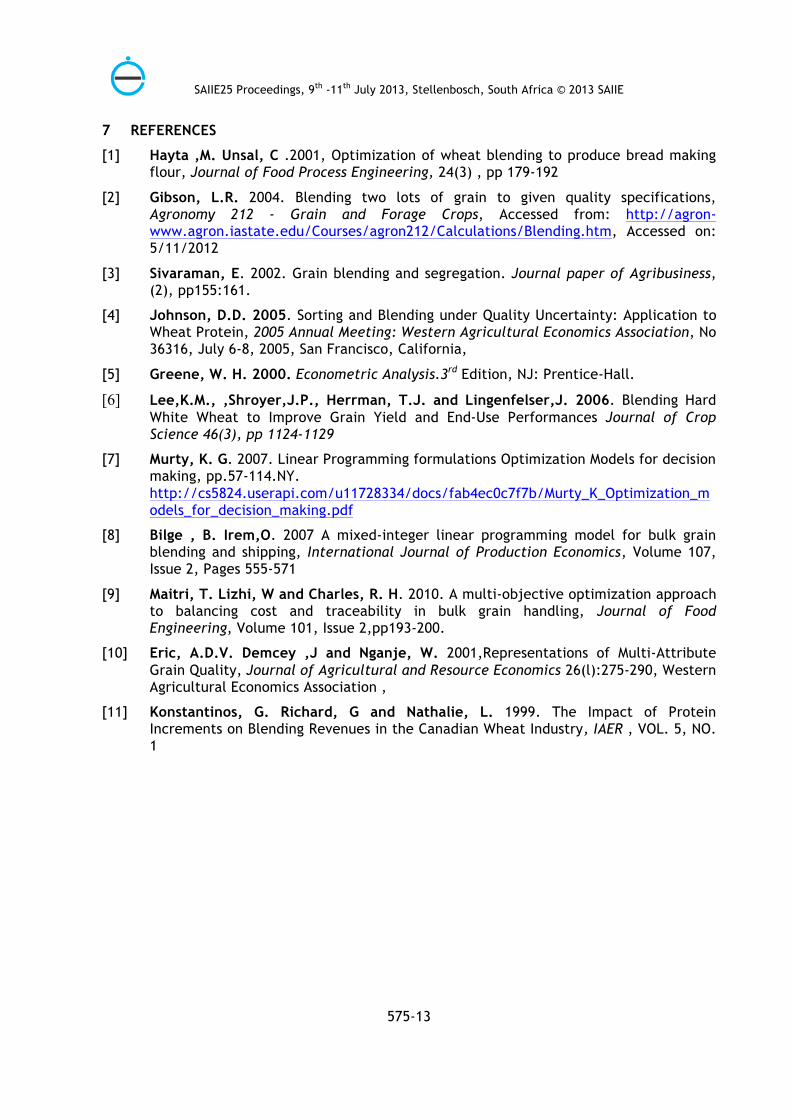
5.1 Application of Malt production in a blending area

We suggest possible application of the LP model in Figure 2. Data is collected from malt analysis. This is loaded in Microsoft Excel, which is linked to a Human machine Interface created using Visual Basics.net. This is then linked to a PLC using Object Process Control (OPC Client/Server).

Visual Basics Human Machine Interface

Microsoft Excel Solver

Silo Status

Silo Discharge

Equipment Status

OPC Client

OPC ITEM

OPC ITEM

OPC ITEM

OPC Server

OPC TAG

OPC TAG

OPC TAG

Programmable Logic

Controller

Equipment

Valves

Sensors

Motors

Relays

Malt Attributes Batch1

Malt Attributes Batch 2

Figure 2 : Application of Linear programming in the control of a blending system

6 CONCLUSION

In this paper, we have offered a general formulation to model grain blending and we emphasized the use of grain quality attributes in determining the optimum quality. Results from the experiments have shown that it is feasible to blend based upon the intrinsic properties of grain as to other constraints from the reviewed authors.

The model based on results presented, shows that it is possible to predict targeted final malt quality properties without the need of analyzing the blended mixture. The model can also be extended (i) to model grain blending decisions based on more than 15 quality attributes because the flexibility of the model allows one to make any alteration quite easily, and (ii) to incorporate uncertainties in measurement of quality attributes. Both of which are avenues inviting further inquiry since the quality attributes used as constraints are determined by both physical and chemical analysis.


575-13

7 REFERENCES

[1] Hayta ,M. Unsal, C .2001, Optimization of wheat blending to produce bread making flour, Journal of Food Process Engineering, 24(3) , pp 179-192

[2] Gibson, L.R. 2004. Blending two lots of grain to given quality specifications, Agronomy 212 - Grain and Forage Crops, Accessed from: http://agron-www.agron.iastate.edu/Courses/agron212/Calculations/Blending.htm, Accessed on: 5/11/2012

[3] Sivaraman, E. 2002. Grain blending and segregation. Journal paper of Agribusiness, (2), pp155:161.

[4] Johnson, D.D. 2005. Sorting and Blending under Quality Uncertainty: Application to Wheat Protein, 2005 Annual Meeting: Western Agricultural Economics Association, No 36316, July 6-8, 2005, San Francisco, California,

[5] Greene, W. H. 2000. Econometric Analysis.3rd Edition, NJ: Prentice-Hall.

[6] Lee,K.M., ,Shroyer,J.P., Herrman, T.J. and Lingenfelser,J. 2006. Blending Hard White Wheat to Improve Grain Yield and End-Use Performances Journal of Crop Science 46(3), pp 1124-1129

[7] Murty, K. G. 2007. Linear Programming formulations Optimization Models for decision making, pp.57-114.NY. http://cs5824.userapi.com/u11728334/docs/fab4ec0c7f7b/Murty_K_Optimization_models_for_decision_making.pdf

[8] Bilge , B. Irem,O. 2007 A mixed-integer linear programming model for bulk grain blending and shipping, International Journal of Production Economics, Volume 107, Issue 2, Pages 555-571

[9] Maitri, T. Lizhi, W and Charles, R. H. 2010. A multi-objective optimization approach to balancing cost and traceability in bulk grain handling, Journal of Food Engineering, Volume 101, Issue 2,pp193-200.

[10] Eric, A.D.V. Demcey ,J and Nganje, W. 2001,Representations of Multi-Attribute Grain Quality, Journal of Agricultural and Resource Economics 26(l):275-290, Western Agricultural Economics Association ,

[11] Konstantinos, G. Richard, G and Nathalie, L. 1999. The Impact of Protein Increments on Blending Revenues in the Canadian Wheat Industry, IAER , VOL. 5, NO. 1


575-14

A LINEAR PROGRAMMING MODEL FOR BLENDING

Documents

Transcript of A LINEAR PROGRAMMING MODEL FOR BLENDING