A limit on eccentricity growth through planet-disc interactions

Alex Dunhill with Richard Alexander & Phil Armitage

1

MotivationExoplanets observed with full range of eccentricities from 0 to ~1.

Formation models agree on a circular disc as the origin of planets.

Parts of distributionwell explained.

Scattering(Jurić & Tremaine, 2008)

Tidal circularisation(Rasio et al. 1996)

???2

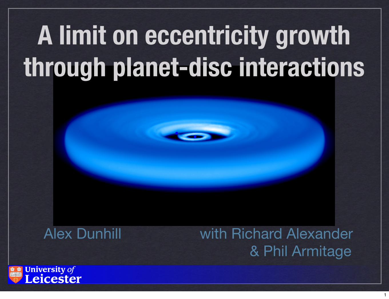
Previous studiesBitsch & Kley (2010) looked at low mass eccentric planets in 3D discs - found e decay.

Papaloizou et al. (2001) and D’Angelo et al. (2006) both explored planet mass.

Both found eccentricity growth.

J. C. B. Papaloizou et al.: Disc and orbital eccentricity growth 265

in the Navier–Stokes equations, even though it probablyarises through complicated processes such as MHD turbu-lence generated by the Balbus–Hawley instability (Balbus& Hawley 1991, 1998).

For computational convenience we adopt dimensionlessunits. The unit of mass is taken to be the sum of the massof the central star (M!) and companion (Mp). The unitof length is taken to be the initial orbital radius of thecompanion, rp. The gravitational constant G = 1, so thatthe natural unit of time becomes

P0/(2!) = ""1 =

!r3p

G(M! + Mp),

with P0 being the initial orbital period of the binary, whichin all cases was initiated on a circular orbit.

2.1. Initial conditions

The disc models used in all simulations had uniform sur-face density, !, with an imposed taper near the discedge, initially. The value of ! was chosen such that whenM! = 1 M#, there exists the equivalent of 2 Jupitermasses (MJ) in the disc interior to the initial orbital radiusof the companion. Then ! = 6 10"4 in our dimensionlessunits.

Di"erent mass ratios between the companion and thecentral star q = Mp/M!, were considered, such that10"3 ! q ! 0.03. For M! = 1 M#, the lower end of thisrange corresponds to a Jupiter mass protoplanet and theupper end to a Brown Dwarf of mass 30 MJ. The innerradius of the disc was located at r = 0.4 and the outerradius at r = 6.

2.2. Boundary conditions

Since material in a viscous accretion disc will naturallyflow onto the central star, an outflow condition was ap-plied at the inner boundary. The outer boundary condi-tion was the same as that described in NPMK.

3. Hydrodynamic codes

The calculations presented here were performed with thethree dimensional MHD code NIRVANA (here adapted to2D) that has been described in depth elsewhere (Ziegler &Yorke 1997). Viscous forces have been added as describedby Kley (1998).

In each case the equations are solved using a finitedi"erence scheme on a discretised computational domaincontaining Nr " N! grid cells, where the grid spacing inthe (r,#) coordinates is uniform.

For the calculations presented here and listed inTable 1, no accretion onto the companion was allowedand three di"erent resolutions have been used. The runwith q = 10"3, listed as N1 in Table 1 used Nr = 130 andN! = 384. The other lower resolution runs used Nr = 200and N! = 200. One higher resolution run used Nr = 400

Table 1. This table lists the label given to each simulation, theresolution used for each calculation (Nr!N!), the companion–star mass ratio, and whether strong eccentricity growth wasobserved

Run Resolution q egrowth?

N1 130 ! 384 10!3 NoN2 200 ! 200 0.01 YesN3 200 ! 200 0.02 YesN4 200 ! 200 0.025 YesN5 200 ! 200 0.03 YesN6 400 ! 400 0.03 Yes

Fig. 1. This figure shows the evolution of the eccentricity ver-sus time (measured in units of P0) for the calculations, N2,N3, N4, N5 listed in Table 1. The lines corresponding to eachcompanion of di!erent mass are indicated on the figure in unitsof MJ

and N! = 400. The numerical method is based on themonotonic transport algorithm of Van Leer (1977), lead-ing to the global conservation of mass and angular momen-tum. The evolution of the companion orbit was computedusing a standard leapfrog integrator.

NIRVANA has been applied to a number of di"erentproblems including that of an accreting protoplanet em-bedded in a protostellar disc (NPMK). It was found togive results that are very similar to those obtained withother finite di"erence codes including FARGO (describedin Masset 2000) and RH2D (described in Kley 1999).

In order to establish the reliability of the numericalresults, simulations were also performed using an alter-native code based on the FARGO fast advection method(see Masset 2000, NPMK). In this scheme, which is able tooperate with longer time steps than NIRVANA, a fourth-order Runge Kutta scheme was used as orbit integrator.Results obtained with the two codes were very similar.

4. Numerical calculations

Recent simulations of protoplanets with 0.001 < q < 0.01,interacting with discs with physical parameters similar to

errors in the planet’s orbital evolution. All calculations presentedin this section employed grid GS2, except for the 3MJ cases oninitially circular orbits (e0 ! 0), which employed grid GS1. Inorder to analyze the orbital evolution of the planet after release,we calculated the osculating elements of the orbit every fewhydrodynamic time steps (approximately every 0.01 orbits). Toremove short-period oscillations, we computed the mean orbitalelements (Beutler 2005) by using an averaging period of oneorbit. Throughout the paper, the planetary orbital eccentricitiesand semimajor axes in the simulations refer to the mean orbitalelements.

5.1. Orbital Eccentricity

Simulations by Papaloizou et al. (2001) showed that the in-teraction between an initially circular disk and a circular-orbitplanet with mass k20MJ can lead to the growth of disk eccen-tricity and planetary orbital eccentricity. They also found thatthis interaction can be more efficient at augmenting orbital ec-centricity than direct wave excitation at the outer 1 : 3 Lindbladresonance in a noneccentric disk (e.g., Artymowicz 1992). Weaim at determiningwhether a similar phenomenon can occur alsoin the Jupiter-mass range.

Figure 8 shows that the interaction between a planet and adisk leads to orbital eccentricity growth for the 2MJ (dashedline) and 3MJ (solid line) cases. During the initial growth of e forthe 3MJ planet, the rate is e " 1:3 ; 10#4 per orbit. This value is$1.6 times that exhibited by the 2MJ planet. The eccentricitygrowth stalls when e ’ 0:08 for both planetary masses. Theplanets may be experiencing some variation in their eccentricityforcing due to the phasing of their eccentricities relative to thoseof the disks. After 1500Y1600 orbits from the release time, theorbital eccentricity starts to increase again with a growth time-scale that is comparable to the initial growth timescale, !E %e/jej " 2:3 ; 103 orbits, for both planetary masses. The averagegrowth timescale is shorter than the standard type II migration (orviscous diffusion) timescale (see x 5.2). Over the last 1000 orbits ofthe simulation, the eccentricity of the 3MJ planet increases veryslowly, at a rate of e " 2 ; 10#6 per orbit.

The model withMp ! 1MJ and initial zero eccentricity (Fig. 9,dashed line) shows a much slower orbital eccentricity growth,reaching e ! 0:02 after 3000 orbits from the release time. Asdescribed in x 4.3, the eccentric perturbation induced by the planeton the disk is also rather weak compared to that excited by the2MJ planet. At the average growth rate of e " 7 ; 10#6 per orbit,it would take on the order of the viscous diffusion timescale toreach e " 0:1.

In order to evaluate the extent of the orbital eccentricity growth,we used configurations with fixed nonzero planetary eccentricitiesprior to release, e0. Figure 9 also shows the orbital eccentricityevolution of aMp ! 1MJ planet with e0 ! 0:01. After release, eoscillates about the initial value. The oscillation grows in ampli-tude and, during one of these cycles, e increases from 0 to 0.09within about 1300 orbits. In this case, !E is of order the viscousdiffusion timescale. We simulated several models with e0 & 0:1(not plotted) and found that there was generally a reduction ofthe orbital eccentricity, albeit with some exceptions. For exam-ple, in amodelwith a 1MJ planet and e0 ! 0:1, e underwent small-amplitude oscillations about the initial value, with periods of a fewhundred orbits. This occurrence may be related to the relativelylarge eccentricity driven in the outer disk. Somemodels with e0 &0:2 showed a rate of change of e that diminishes in time. Inthese cases the evolution was generally monitored for less than1000 orbits. Longer time coverage simulations are required toassess the long-term behavior of these configurations.

5.2. Radial Migration

We describe here some results on the migration of eccentric-orbit planets. We plan to explore this issue further in a futurepaper. Radial migration of planets in the mass range consideredin this study is expected to be in the standard type II regime, whichis characterized by an orbital decay timescale !M % a0 / aj j !2a2

0 /(3") ! ! IIM (Ward 1997). The type II migration rate depends

only on the viscous timescale of the disk near the location of theplanet and is independent of the disk density, provided the diskis locally more massive than the planet. Type II migration is

Fig. 8.—Evolution of the (mean) orbital eccentricity of 2MJ (dashed line)and 3MJ (solid line) planets after the release time, trls ! 1000 orbits.

Fig. 9.—Orbital eccentricity vs. time of Jupiter-mass models with differentinitial orbital eccentricities: e0 ! 0 (dashed line) and e0 ! 0:01 (solid line). Therelease time is 1100 orbits.

EVOLUTION OF GIANT PLANETS IN ECCENTRIC DISKS 1707No. 2, 2006

But in 2D, grid hydro, high surface density discs.3

Method

High resolution (107 particle) 3D SPH simulations using GADGET-2.

Directly calculates gravity for planet and star.

Locally isothermal equation of state.

High mass planet, varied surface density profiles.

Explicit Navier-Stokes viscosity (α = 10-2).

4

MOVIES OF THESE SIMULATIONS CAN BE FOUND AT

HTTP://WWW.ASTRO.LE.AC.UK/~ACD23/ECCENTRICITY.HTML5

Simulation resultsRun 7 models.

Eccentricity only grows for Σ > 103.

6

Planet mass vs. surface densityCombining results with previous studies yields:

7

Planet mass vs. surface densityCombining results with previous studies yields:

? ? ? ? ? ? ? NO

NO?

YES, BUT...

7

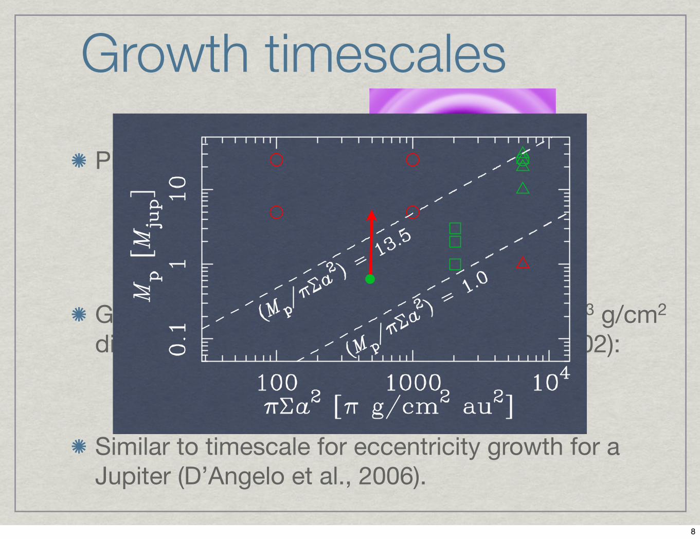
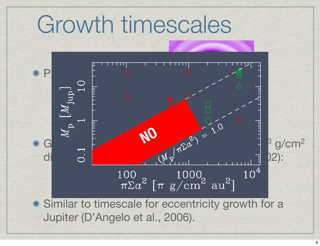
Planets in gaps accrete:

Growth timescale for giant planet in a Σ~102-3 g/cm2 disc (Lubow et al., 1999; D’ Angelo et al., 2002):

Similar to timescale for eccentricity growth for a Jupiter (D’Angelo et al., 2006).

Growth timescales

⌧accrete . 104�5 tdyn

8

Planets in gaps accrete:

Growth timescale for giant planet in a Σ~102-3 g/cm2 disc (Lubow et al., 1999; D’ Angelo et al., 2002):

Similar to timescale for eccentricity growth for a Jupiter (D’Angelo et al., 2006).

Growth timescales

⌧accrete . 104�5 tdyn

8

Planets in gaps accrete:

Growth timescale for giant planet in a Σ~102-3 g/cm2 disc (Lubow et al., 1999; D’ Angelo et al., 2002):

Similar to timescale for eccentricity growth for a Jupiter (D’Angelo et al., 2006).

Growth timescales

⌧accrete . 104�5 tdyn

NO

8

ConclusionsNo e growth for canonical disc parameters.

For high mass planets, need high surface density in disc to grow eccentricity.

For low mass planets, , so quickly move outside region of allowed eccentricity growth.

⌧accrete ⇠ ⌧ecc

We conclude that this is notan efficient process for growing

planetary eccentricities:Some other mechanism!

Dunhill, Alexander & Armitage 2012 (submitted)

9