
A Lecture on Low Consistency Refining of Mechanical Pulp
44
1 A Lecture on Low Consistency Refining of Mechanical Pulp James A. Olson Pulp and Paper Centre, Department of Mechanical Engineering, University of British Columbia Outline: what we will cover today LC refining equipment and overview Fibre morphology changes Characterization of the refining effect Total energy transfer, no load, refiner efficiency Intensity of energy transfer Heterogeneity of treatment Fibre cutting during LC refining
Transcript of A Lecture on Low Consistency Refining of Mechanical Pulp

1
A Lecture on Low Consistency Refining of Mechanical Pulp
James A. Olson
Pulp and Paper Centre,
Department of Mechanical Engineering,
University of British Columbia
Outline: what we will cover today
LC refining equipment and overview
Fibre morphology changes
Characterization of the refining effect
Total energy transfer, no load, refiner efficiency
Intensity of energy transfer
Heterogeneity of treatment
Fibre cutting during LC refining

2
LC Refining
LC refiners operate at 3-5% consistency
Differs from HC refining in that:
Pump through operation
Decouples the flow in the refiner from refiner operation
and design (speed / diameter / plate geometry)
Smaller, more controlled plate gap than HC refiners
No steam production
LC Refining
Conventional LC refining done in stock prep
area of papermachine
Originally chemical pulp
Increase pulp strength,
sheet smoothness
Increasingly important
in the manufacture of
mechanical pulp

3
LC Refining
Flow in a LC refiner
Conical Refiner
Double Disc
LC refining
Bars
Fibre capture and transport
Cyclic compression and shear
Permanently deforms fibre wall
Grooves provide capacity
Angles provide uniform bar
contact area
Page - 1985

4
LC Refining - paper properties
Fibre flexibility and higher
bonded area increases sheet
strength
More flexible fibres increase
sheet smoothness
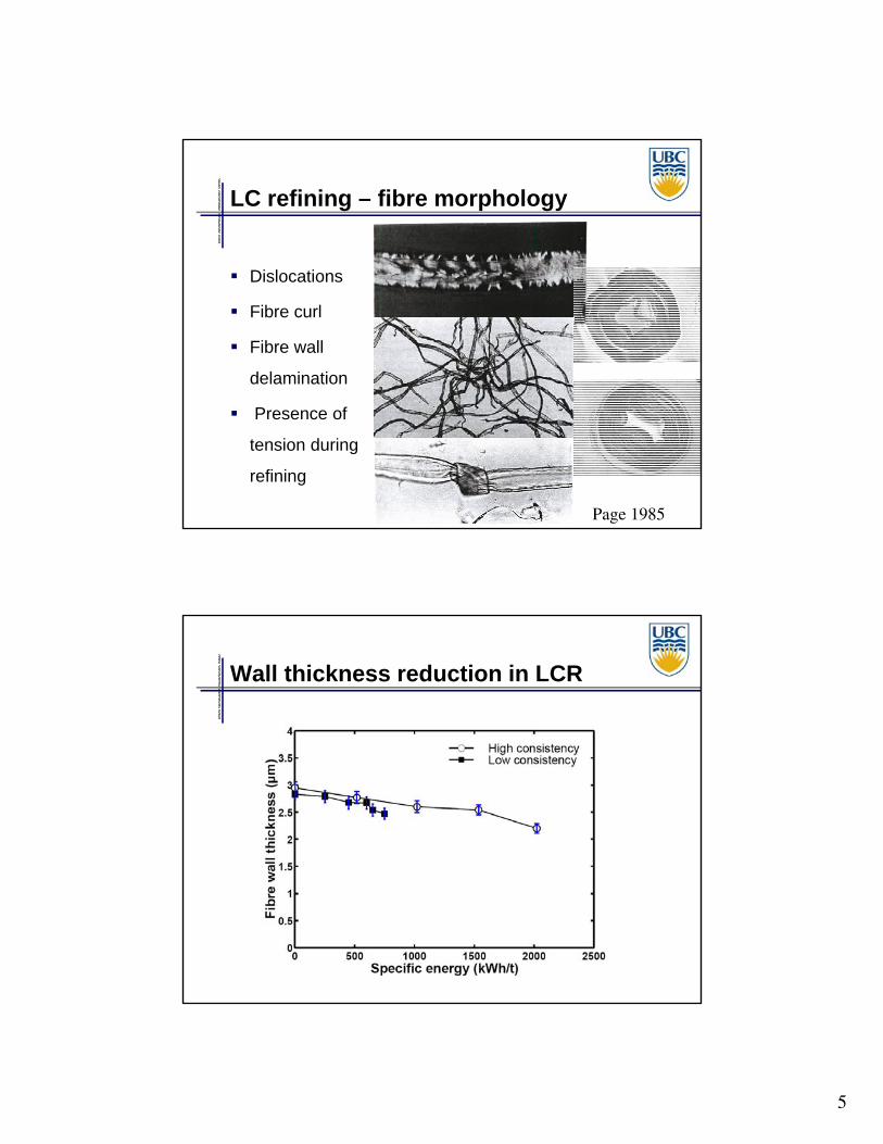
LC refining – fibre morphology
Imposes cyclic compression on fibres
Internal delamination – break down of
cell wall – increases flexibility
External fibrillation – increases
relative bonded area
Reduces wall thickness - increases
fibre flexibility, fines production
Fibre cutting
5
LC refining – fibre morphology
Dislocations
Fibre curl
Fibre wall
delamination
Presence of
tension during
refining
Page 1985
Wall thickness reduction in LCR

6
LC refining in mechanical pulping
Mechanical pulping has traditionally only
used high consistency (HC) refining
Low consistency refiners are used in 3 main
areas
Reject refining
Post refiners
(Low consistency) Third stage refining
LC reject refiners
Effective at removing shives
Significant energy savings
Minimum capital investment
Limit to the amount of energy
that can be transferred to the
pulp before fibre cutting
Good for lower grades of
mechanical pulp …

7
LC reject refiners Port Hawkesbury – Newsprint (blended into SCA)Lowest capital cost per ton of any modern TMP mill (900 admt/d:C$90M)
Mokvist et al, IMPC – Norway, 2005
LC mechanical pulp post-refiners
Located in papermachine stock prep area
Small freeness change, low tear loss, relatively small tensile
improvement
Coupled to papermachine to facilitate immediate response to
changing pulp quality
Enables better pulp quality control
Freeness at TMP disc thickener is higher
Not typically used for energy reduction or capacity increase

8
LC refining – third stage refiners
High Consistency (HC) 20-40%
Primary Refiner(HC)
Chip feeder
Tertiary Refiner(LC)
Secondary Refiner(HC)
Low consistency (LC) 3-4%
Latency removal
LC refining – third stage refiners
LCR add 5% of total energy applied to pulp
typically 100-150 kWh/t.
Increased production for minimum capital investment,
typically, 10% increase in production for northern softwood
Decrease shive content
Allow for low latency residence time
Improve pulp quality, improve tensile at slightly lower
Freeness
Energy reduction, typically 5-7% savings
Note: Energy, capacity and quality are trade-offs

9
LC refiners – energy savings potential
Sabourin et al, 2007 IMPC
HCR HCR+LCR
LC refiners – energy savings potential
Sabourin et al, 2007 IMPC
HCR HCR+LCR
10
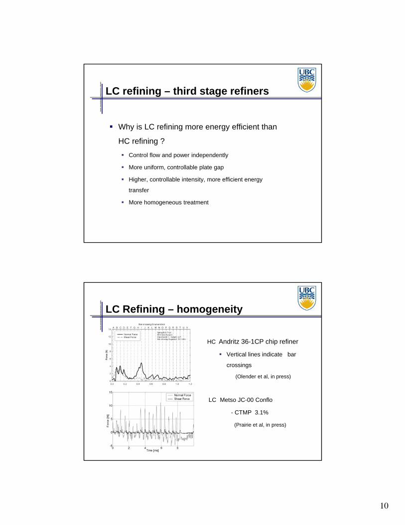
LC refining – third stage refiners
Why is LC refining more energy efficient than
HC refining ?
Control flow and power independently
More uniform, controllable plate gap
Higher, controllable intensity, more efficient energy
transfer
More homogeneous treatment
LC Refining – homogeneity
HC Andritz 36-1CP chip refiner
Vertical lines indicate bar
crossings
(Olender et al, in press)
LC Metso JC-00 Conflo
- CTMP 3.1%
(Prairie et al, in press)

11
LC refiners – energy savings potential
Strategy to increase energy to LC refiners and
reduce energy to HC refiners
What limits the energy saving potential of LC
refiners?
As power increases so does “Intensity” of treatment
As Intensity increases fibres become increasingly broken / cut.
At high power you get an unacceptable loss in pulp tensile
strength.
LC Refiner characterization
E - Specific energy: Total amount of energy transferred to the
pulp per unit mass.
P [kW] power applied to the refiner
Pno-load [kW]
Power applied before fibre quality begins to change.
Many people use a rule of thumb 0.050 inch (1.25mm) gap
Pnet = P – Pno-load Net power is the power that goes to the pulp
Measured with pulp moving through refiner
= [o.d. tonnes / day] Mass flow rate of pulp.
M
PPE loadno
M

12
No-load power
HC refining no load is small / negligible
Steam provides small viscous drag on plate
LC refining no load power can be significant
Can be up to 40% of total power
High viscous friction in 4% pulp suspension
Power – plate gap
0
500
1000
1500
2000
2500
0 1 2 3 4 5 6 7 8 9 10 11
Tota
l pow
er, k
W
Gap, mm
No-load ?(500kw)
Current operation(1200kw)
58 inch LC twin flow refiner, 4% consistency TMP

13
Refiner Efficiency
If the refiner is not fully loaded than the efficiency of
the process can be very low.
Refiner Efficiency
The previous power curve showed that current operating power is
1200kW and the no load power is approximately then the efficiency
would be
Only 37% of the energy is transferred to the pup.
%5.371200
7501200
E
PowerTotal
PowerNet E
No – load power correlation
From fluid dynamics a dimensional analysis
suggests that Pno-load should be
Cp = power coefficient, approximately constant
N = RPM (Angular velocity)
D = Diameter of plate
= fluid density
Approximately independent of flow rate
Other published correlation:No load power = k * D4.3 * N3
53DNCP ploadno 53DN
PC loadno
p
Example, Herbert and Marsh 1968

14
Energy saving opportunity Reduced periphery plate
58 inch no-load is
477kW
55 inch no-load is
307 kW
No-load reduced by
approx 170 kW or
35% reduction in no-
load
No loss is tensile
strength 39
40
41
42
43
44
45
46
47
48
0 20 40 60 80 100 120 140 160
Ten
sile
Ind
ex (N
m/g
)
Specific Energy Consumption (Kwh/ton)
TSR3
TSR4
58 inch plate
55 inch plate
Refiner efficiency
LC refiners should be operated at full power
to increase efficiency
Optimize plate design and geometry to enable fully
loaded operation
Utilize reduced periphery plates
Shutdown refiners in parallel
Need to optimize plate and HC operation to
enable full power to LC refiners

15
Specific energy ranges
E Specific energy: Total amount of energy
transferred to the pulp per unit mass. M
PPE loadno
Grade Pulp kWh/t
Fine Papers Hardwood 80-120
Softwood 80-140
News/directory SW Kraft 40-100
Post-refineTMP 20-60
TSR 60-120
Linerboard OCC 30-60
Refining intensity
Specific Energy is not enough
Need to describe intensity of treatment
Range of 2-parameter characterizations (energy and intensity)
Energy can be expended in different ways
Large number of low energy impacts
Small number of large energy impacts
Break energy down into these components (Number and
intensity).
16
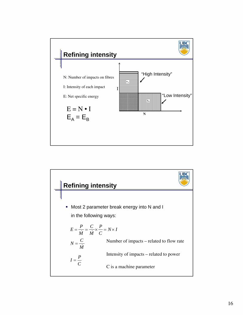
Refining intensity
I
“High Intensity”
BE
AE
“Low Intensity”
N
N: Number of impacts on fibres
I: Intensity of each impact
E: Net specific energy
E = N • IEA = EB
Refining intensity
Most 2 parameter break energy into N and I
in the following ways:
INC
P
M
C
M
PE
M
CN
C
PI
Number of impacts – related to flow rate
Intensity of impacts – related to power
C is a machine parameter

17
Refining intensity
Specific Edge Load theory
C is the “Cutting edge length” CEL
CEL is the total length of bar edges a fibre
will see in a revolution [km/rev]
i
srR
R
sr rnn
drnn
CEL ii
coscos
2
1
TAPPI – technical information sheet
CEL= Number of bars on rotor X no of bars on stator X bar length divided by cosine of bar angle to radius
Refining intensity Cutting edge length
Example of using the
discrete form of the
equation
Divide disc up and count …
i
srR
R
sr rnn
drnn
CEL ii
coscos
2
1

18
Refining intensity
Integral example …
Can re-write integral in terms of bar width
and groove width, i.e,
2
31
32
22
1
22
3cos
2
cos
2
wg
RRdr
wg
rCEL
R
R
gw
rrnr
2)(
gw
rrns
2)(
Refining intensity
Specific Edge Load [J/s]
Although derived empirically, in rigorous terms SEL is
the energy expended per bar crossing per unit bar
length ( Kerekes and Senger, 2006)
CEL x RPM=SEL is the “machine parameter” –
Specific-edge-Load
SEL is not directly the energy expended on pulp
CELRPM
P
SEL
PI

19
Refining intensity
Example plate pattern
ICPM
Refining intensity
Typical specific edge loads for various paper
grades

20
Other “Machine Intensities”
Specific Surface Load LUMIAINEN, 1990
Modified Edge Load MELTZER F.P., RAUTENBACH R., 1994,
( . . )
. 2 tan
Bar width groove widthXSEL
bar widthX
.
SEL
bar width
Specific Surface Load
Accounts for bar
width
Considered to
be energy per
unit area of bar
surface
2
Specific Edge LoadSSL
Bar WidthW s 1 W s
m m m
2/J m

21
“Fibre Intensity”
“Fibre Intensity” is the energy expended on
pulp by bar crossings
It requires assumptions about how fibres are
captured from grooves and impacted during
bar crossings
It is a “Specific Energy per Impact”, S
Probability of Fibre Impact
SEL is the energy expended per bar crossing per unit
bar length … don’t know how much pulp that energy is
expended on …
Not all fibres are impacted in every bar crossing
Can show this readily from mass balance of fibres in
groove vs. fibres in gap
C-Factor used to estimate fibre captured

22
Fibre capture zoneKerekes & Olson (2003)
From mass balance, only about 5-10% of pulp in groove can fit in gap.
C Factor for Disc Refiner
Dw
RRtannCGDC F
3218 3
132
32
C
PI
23
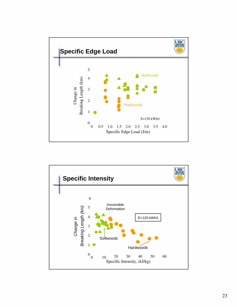
0 0.5 1.0 1.5 2.0 2.5 3.0 3.5 4.00
1
2
3
4
5
Specific Edge Load (J/m)
Cha
nge
in
Bre
akin
g L
engt
h (k
m) Softwoods
E=120 kWh/t
Hardwoods
Specific Edge Load
6
0 10 20 30 40 50 600
1
2
3
4
5
Specific Intensity, (kJ/kg)
Cha
nge
in
Bre
akin
g Le
ngth
(km
)
E=120 kWh/t
IrreversibleDeformation
Softwoods
Hardwoods
Specific Intensity

24
Comparison of Intensities
J.C. Roux (FRS Oxford 2009)
Recently a comparison of intensity estimates
Specific Edge Load (SEL), Specific Surface Load (SSL), Modified
edge load (MEL) and his own Net Normal Force per Bar Crossing
Gives correlations to fibre cutting for each intensity
Comparison of Intensities
J.C. Roux (FRS Oxford 2009)

25
Comparison of Intensities
Demonstrates that:
Roux / Kerekes: SEL is not a great predictor of refining effect
Roux: MEL is a better predictor
Kerekes: C-factor is better than SEL
Roux: Net normal force per bar crossing gives best correlation
Problem is that it is difficult to measure effect of
intensity … need to measure a pulp property
interpolated to a Specific Energy
Our recent work …
We hypothesize that Intensity is directly
proportional to the refiner gap
Gap is easily measured
Power is proportional
to 1/Gap
Not the first to say this
Ulla-britt Mohlin (2005)
Miles, May, et al (1987) on
reject refiner

26
Vary Total Energy Applied
Specific energy
• 60 kWh/t increments from 0 to 420 kWh/t
Vary Intensity
Specific Edge Load (SEL) [J/m]
• 0.14 (low), 0.28 (medium), 0.56 (high)
Vary plate geometry (BEL) [km/rev.], flow rate
[kg/s], power [kW] and RPM [1/s]
Achieve intensities with several combinations
Measure pulp quality response
Pilot Trials
Andritz R&D laboratory Springfield OH
22 inch TwinFlow refiner
Trial plan

27
Results, Freeness-SE
0
20
40
60
80
100
120
140
0 50 100 150 200 250 300 350 400 450
CSF [ml]
Specific Energy [kWh/t]
Results, Tear-Tensile
3
4
5
6
7
8
9
10
11
40 45 50 55 60 65
Tear In
dex [mNm
2/g]
Tensile Index [Nm/g ]
High Intensity
Low Intensity

28
Results, Tensile-Intensity
‐2
0
2
4
6
8
10
12
0 0.1 0.2 0.3 0.4 0.5 0.6
Tensile increase [Nm/g]
@ 200 kWh/t
Intensity [J/m]
Results, Tensile-Gap
‐1
0
1
2
3
4
5
6
7
8
9
0 0.05 0.1 0.15 0.2 0.25 0.3 0.35 0.4 0.45 0.5
Tensile increase [Nm/g]
@ 200 kWh/t
Gap [mm]
Fibre cutting Elastic deformation
Fibrillation
29
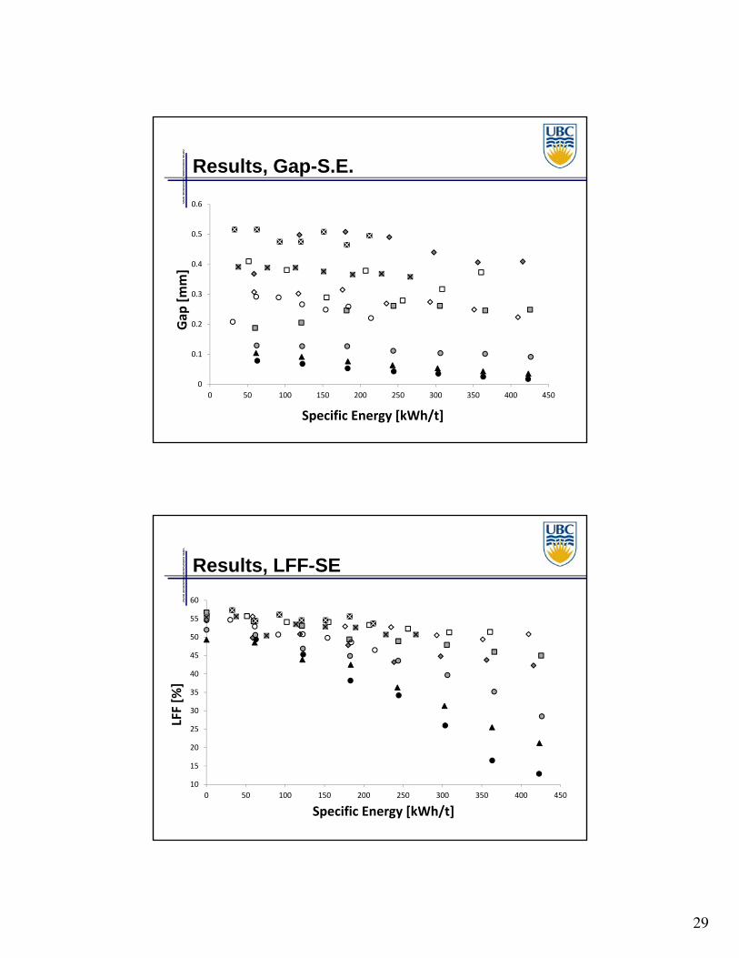
Results, Gap-S.E.
0
0.1
0.2
0.3
0.4
0.5
0.6
0 50 100 150 200 250 300 350 400 450
Gap
[mm]
Specific Energy [kWh/t]
Results, LFF-SE
10
15
20
25
30
35
40
45
50
55
60
0 50 100 150 200 250 300 350 400 450
LFF [%
]
Specific Energy [kWh/t]
30
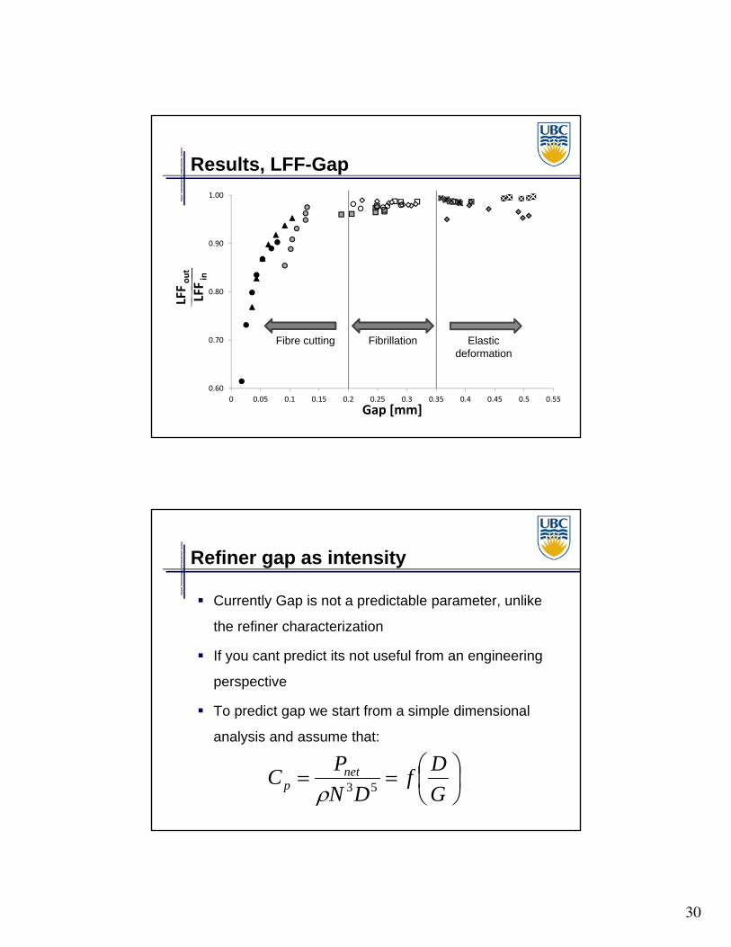
Results, LFF-Gap
0.60
0.70
0.80
0.90
1.00
0 0.05 0.1 0.15 0.2 0.25 0.3 0.35 0.4 0.45 0.5 0.55
LFFout
LFFin
Gap [mm]
Fibre cutting Elastic deformation
Fibrillation
Refiner gap as intensity
Currently Gap is not a predictable parameter, unlike
the refiner characterization
If you cant predict its not useful from an engineering
perspective
To predict gap we start from a simple dimensional
analysis and assume that:
G
Df
DN
PC net
p 53

31
Results, Power Number-Gap
0
0.001
0.002
0.003
0 1000 2000 3000 4000 5000 6000 7000
Pnetρω3D5
DG
Refining intensity - Gap
Predict Refiner gap from power, speed and size
Refiner gap controls:
Fibre cutting – long fibre content – critical gap
Freeness change
Forgacs (1963) pulp properties can be predicted from
a measure of fibre length and surface area
Use Specific energy and Gap to predict CSF and Length changes
Use CSF and fibre length to predict tear and tensile changes

32
Results, Tear-LFF
3
4
5
6
7
8
9
10
11
10 15 20 25 30 35 40 45 50 55 60
Tear In
dex [mNm
2/g]
LFF [%]
Results, Tensile-LFF2/CSF
30
35
40
45
50
55
60
65
70
0 0.003 0.006 0.009
Tensile In
dex [Nm/g]
LFF2[%]CSF [ml]

33
Intensity Summary
Increasing refiner power increases intensity
Several methods to estimate intensity
Plate gap controls intensity of treatment
High normal forces on fibres at smaller gap (Roux)
Force based analysis shows gap controls forces on fibres (kerekes)
Increasingly active area of research
Implies:
Operate LC refiner at highest possible power (smallest gap) before onset of
cutting
Gap measurement and control is increasingly important
HETEROGENEITY OF REFINING
66
34
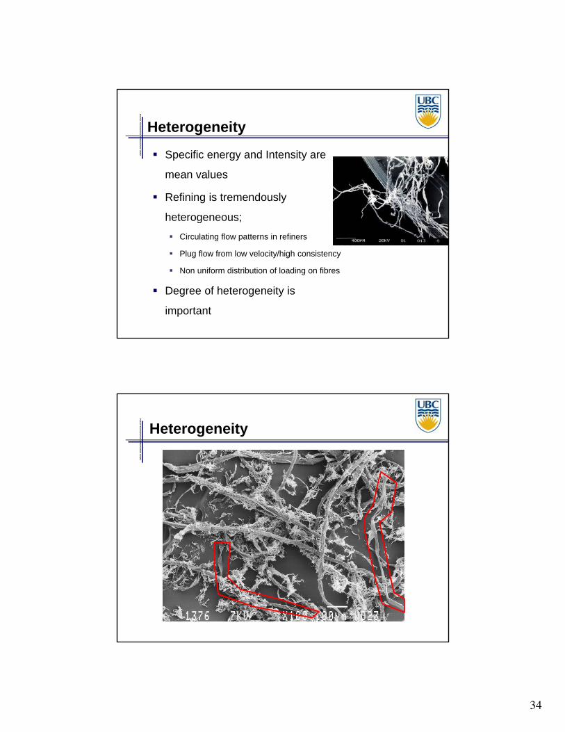
Heterogeneity
Specific energy and Intensity are
mean values
Refining is tremendously
heterogeneous;
Circulating flow patterns in refiners
Plug flow from low velocity/high consistency
Non uniform distribution of loading on fibres
Degree of heterogeneity is
important
Heterogeneity

35
Heterogeneity
Model refining experiment –
compression refiner
Only a fraction of the fibres
are compressed / refined
On repeated compression cycles the same
fibres are refined .. No change in tensile
Fibres redistributed … new fibres are
refined and continuous change in tensile
MTS compression tester and test cell.
Heterogeneity
0.0
1.0
2.0
3.0
4.0
5.0
0 50 100 150 200
No. of Cycles
Bre
ak
ing
Le
ng
th (
km
)
Without Redistribution
Redistribution After Every Cycle

36
Heterogeneity
Results of single fibre compression studies showed that (P.
Wild et al 2001):
Fibre modulus changed during first compression and no subsequent
change after that.
We postulate that small fraction of fibres, P, are refined
during any one cycle in our refiner
Statistical Analysis: fraction of refined fibres after n cycles:
Tensile increase is proportional to fraction of refined fibres
1 1n
R n P
Heterogeneity
1.8
2.3
2.8
3.3
3.8
4.3
4.8
0 10 20 30 40 50
Cycles
Bre
akin
g L
eng
th (
km)
0.0
0.2
0.4
0.6
0.8
1.0
Pro
bab
ilit
y
Compression Refining Trials
Cumulative Probability of a Fibre Being Refined

37
Heterogeneity
From this analysis we can predict the probability of a
fibre being refined during each compression:
P = 0.06
Similar analysis can be performed for a disc refiner
assuming a bar crossing is a compression cycle.
Heterogeneity
Similar analysis for LC
refiner
P=0.0021
Large number of bar
crossings
Small number of fibres
affected during each rbar
crossing
2.7
3.7
4.7
5.7
6.7
7.7
8.7
0 100 200 300 400 500 600 700 800 900
Number of bar crossings, N B [-]
Bre
akin
g L
eng
th [
km]
0.0
0.1
0.2
0.3
0.4
0.5
0.6
0.7
0.8
0.9
1.0
R(N
B)
[-]
C=2%; SEL=2J/m
Commulative probability of fibre being refined
0021.0P
BNB PNR 11

38
Heterogeneity - Summary
Small number of fibres are impacted during each
bar crossing
Large amount of heterogeneity. Some fibres remain unrefined.
Large number of bar crossing are required to
ensure sufficient fraction of pulp is refined.
Opposed to the fatigue hypothesis of fibre deformation used by
many
FIBRE CUTTING

39
Fibre cutting model
Want to understand fibre cutting because it
limits the application of LC refining.
Want to know
What fibres are cut?
How does specific energy determine cutting?
How does intensity affect cutting?
Fibre Comminution
Comminution model adapted from crushing and grinding industries to describe fibre length reduction using the following equation:
Ni = Fibre length distribution E = Specific Energy (kWhr/t) Si = Selection function (Cutting rate)Bij = Breakage function
jjij
ijiii NSBNS
dE
dN
2
0100200300400500600700800900
1000
0.00 1.00 2.00 3.00 4.00 5.00
N
Fibre Length (mm)
Olson, et al 2001Heymer, 2009

40
Initial Validation Experiments
Test the experimental and computational
methodology
Handsheets made from the same
chemical pulp
Handsheets cut into strips of varying
width:
2mm, 5mm, 7mm
Fibre length measured before and after
And S calculated from fibre length
distributions
Exclude fibres less than 0.5mm
Validation Results
Fibre cutting is function
is linear with fibre length
Measured cutting is
smaller than theory

41
Experimental
Pilot Refining trials 5 different plate patterns 2 different refiners (22” Beloit DD, EW) Range of Consistencies, Energy, Flowrates
Fibre length distribution measured using an optical fibre analyzer
Calculate Si numerically knowing the fibre length distribution and the applied energy
Pilot Refining Experiments
Determine selection function for:
Increasing specific energy at a constant intensity
Increasing SEL at a constant specific energy
Varying SEL and refiner plates and refiners
Examine relationship between cutting and
tensile strength

42
Varying Specific Energy
How:
Vary mass flow rate
Constant cconsistency, power
High intensity plate
Probability of cutting per kWh/t is
Pproportional to fibre length
Independent of specific energy
Fibre cutting is not a fatigue
process
Varying SEL
How: Vary applied power Constant Specific energy
(120 kWhr/t)
Cutting is dependent on SEL
Cutting independent of consistency
Cutting proportional to length Propose to characterize
Cutting by constant of proportionality
ii LS

43
All Trials
Vary SEL by
Power
Plate type
Refiner type
Constant specific energy
(120 kWhr/t)
Cutting a function of SEL
Independent of consistency
Tensile Strength
Constant specific energy,
120kWhr/t
Small cutting rate strength
increases
Large cutting rate strength
decreases
Not a great correlation
Same cutting, significant
changes in tensile
44
Conclusions
Developed experimental and computational methods to measure fibre cutting distribution
Fibre cutting is Proportional to fibre length
• Implies random cutting process
Proportional to specific energy• More energy more cutting• Not a fatigue process
Function of refining intensity (SEL) Independent of consistency
Developed a predictive model of fibre length distribution changes during refining
Optimal tensile strength development may be at the onset of fibre cutting