A Latent Measure of Political Protest∗

Erica Chenoweth†, Vito D’Orazio‡, and Joseph Wright§

March 25, 2014

Prepared for the Annual Meeting of the International Studies Association

March 29, 2014 (Toronto, ON)

Abstract

In recent years, scholars have developed a number of new databases with which to measureprotest. Although these databases have distinct coding rules, all attempt to capture incidentsof social conflict. We argue, however, that due to a variety of sources of measurement error,subjective coding decisions, and operational specifications, no single indicator of protest ade-quately measures how much protest exists in a given place at a given time. As a result, empiricalstudies that employ these measures yield inferences with limited generalizability. To increasethe generalizability of the empirical findings, we suggest using an Item Response Theory (IRT)approach to estimate a latent dimension of protest using nine different protest measures thatvary in their operational specifiations as well as their temporal and spatial coverage. The es-timates of the IRT models are used in two ways. First, to demonstrate how existing measuresdiffer, the IRT’s item estimates are used to compare the nine measures of protest based on theirdegree of diffculty (the quantity of latent protest required to observe a ‘1’ in the data) and theirability to discriminate (the speed with which changes in the latent quantity of protest affect theprobability of observing a ‘1’ in the data). Second, the estimated quantity of protest is appliedto both monthly and yearly models of authoritarian breakdown. The results demonstrate thatthe latent protest variable increases the out-of-sample classification of authoritarian breakdownevents; and improves in-sample prediction relative to existing global protest variables. Ourstudy illustrates the potential value of modeling a latent dimension of protest rather than solelyrelying on observed indicators.

∗The author order is alphabetical. This research was conducted for the Political Instability TaskForce (PITF). The PITF is funded by the Central Intelligence Agency (CIA). The views expressedherein are the authors’ alone and do not necessarily represent the views of the Task Force or theU.S. Government.†Email: Erica.Chenoweth@du.edu. Corresponding author.‡Email: dorazio@iq.harvard.edu§Email: josephgwright@gmail.com

When protests began in Ukraine in late 2013, many were wondering what effect they would haveon outcomes such as the durability of the regime, regional power relations, and future internationalinfluences on the country. A common response to these questions is that it depends on how muchprotest we observe. Indeed, in recent years, scholars have developed a number of new databaseswith which to measure protest.1 Although these databases have distinct coding rules, all attemptto capture incidents of social conflict. Yet, reliably observing the quantity of protest in a countrypresents numerous challenges. We argue that due to a variety of sources of measurement error dueto media coverage, subjective coding decisions, and operational specifications, no single indicatorof protest adequately measures how much protest exists in a given place at a given time. Thosethat do measure some quantity of protest, such as the Social Conflict in Africa Database (SCAD),are often quite limited in terms of spatial or temporal coverage (Ukraine, for example, is beyondthe scope of SCAD). Moreover, operational definitions of protest, source materials, and codingdecisions may vary widely across protest measures. As a result, empirical studies that employthese measures yield inferences based on the operationalization of an individual measure ratherthan inferences based on the degree of protest.

In many ways, the issue here is similar to measurement of many different types of political phe-nomena, including democracy (Treier and Jackman 2008; Pemstein, Meserve and Melton 2010) andcorruption (Pieroni, d’Agostino and Bartolucci 2013). In all such cases, the indicators commonlyused to represent different classifications of political phenomena – or different political events – arenot observed directly, and are simply operationalized using theoretical assumptions (implicitly orexplicitly). In making these conceptual distinctions, researchers may introduce measurement errorinto the operationalization of these concepts in ways that influence the research findings scholarsproduce when they use these indicators.

In an effort to improve the measurement of protest, we combine nine different protest data setsin an Item Response Theory (IRT) framework to estimate a latent measure reflecting the quantityof protest at two levels of analysis (country-year and country-month). This is a useful approachbecause each dataset relies on different sources – including, in the case of the Major Episodes ofContention Data Project (MEC), news sources supplemented with historical research – such thatcross-validation and inputs of missing information may improve the data’s coverage. The IRTframework also provides a set of item parameters that describe the relationship of these variablesto one another. For example, the analysis of these parameters shows SCAD to be a liberal measureof protest, while MEC is consistently shown as a conservative measure. Banks’ protest measure,the most common in the literature, is somewhere in the middle, but contributes more informationto the underlying latent measure than others.

The IRT models estimate a latent trait for each observation (a quantity of observed protest)that is explored by applying it to a model of authoritarian breakdown. The results demonstratethat the latent protest variable increases the out-of-sample classification of authoritarian breakdownevents; and improves in-sample prediction relative to existing global protest variables. Our studyillustrates the value of modeling a latent variable rather than solely relying on observed indicatorsof protest.

1See Appendix for a full discussion of the protest variables.

1

Weaknesses of Observed Protest Indicators

Individual attempts to measure a quantity of social protest may be inadequate for three reasons:measurement error due to media coverage, subjective coding decisions, and varying operationalspecifications. Even in cases where efforts are made to avoid measurement error, minimize sub-jectivity, and generalize the concept to a degree where various operational specifications can beobtained using the same data, there are often limits to the scope of coverage. As a result, theinferences we draw from empirical models are tied to the idiosyncrasies of the protest measure,with varying generalizability to the latent concept of interest.

There are three primary sources of measurement error due to media coverage. First, scholarshave long noted a tendency for the news media to under-report nonviolent events, like protests,compared with violent ones, like bombings or attacks (Smith et al. 2001). Because news sources(e.g. newspapers and newswires) are the most common source from which protest researchersdevelop these databases, such datasets may not represent the full universe of events – a problemthat is particularly acute in protest data sets that rely on a single news source, such as the NewYork Times. Such data sets quite literally only capture protests “observed by a New York Timesreporter,” which limits the reliability of such indicators when considered in isolation from othernews reports.

A related problem is that the systematic under-reporting of protest events in single news sourcesis probably even more pronounced than for violent incidents, since information on nonviolent actionis arguably much easier for governments to suppress. It is likely easier to deny a protest by unarmedpersons than an armed attack, particularly when the protest is relatively small or subtle. Forinstance, Herkenrath and Knoll (2011) find that protest databases that rely solely on internationalmedia sources – as do Banks and SCAD – systematically under-report protest activity in somecountries, where such coverage is generally lacking due to disinterest or censorship.

Third, many forms of protest – such as everyday forms of resistance, certain symbolic protests,and stay-at-home demonstrations – are unlikely to obtain meaningful news coverage, at least onan incident-level basis (Scott 1985). This means that news coverage tends to converge on large,spectacular, and visually-stimulating forms of protest while ignoring more mundane, day-to-dayforms. Yet the latter can often be highly influential in developing the capacity and “cognitiveliberation” for a larger social movement to emerge (McAdam 1999). Moreover, this bias rendersinaccurate claims that existing protest databases capture all protest incidents; we know, or at leastwe suspect, that they systematically undercount contentious activity in other forms. Because ofthese problems, some data sets rely on both international and local news reports (e.g. Regan), orthey supplement news reports with additional historical research (e.g. MEC). This provides an op-portunity to leverage information from data sets relying on different source material to compensatefor potential measurement error through under-reporting.

Subjective coding decisions represent another mechanism by which individual measures ofprotest may be inadequate for measuring the degree of protest. For example, existing datasetsmay draw on different primary and secondary sources in an attempt to mitigate the effects ofsystematic media bias. Source selection is subjective, however, and ultimately this decision mayinduce any or all of the three types of measurement error described above.

More generally, subjective coding decisions are made whenever the operational definition lacksthe ability to clearly delineate an observation. Regardless of how precise the operationalizationis, subjectivity creeps into the data in this way. In such instances, the decision to include theobservation, or to assign a score to that observation, is a function of the principal investigator or

2

research assistant more than anything else. Using a variety of measures may help yield consensuson such observations, even if the estimated latent quantity has larger confidence intervals thanobservations for which there is more consistency.

A third issue when measuring protest is that operational specifications differ from measureto measure. While this feature is certainly not unique to protests, it appears to be exceedinglyproblematic in this literature. For example, a SCAD protest can consist of fewer than 10 indi-viduals while an MEC protest requires a minimum of 1,000. While such definitions are typicallyclear, it is difficult to quantitatively assess the effect of a protest when the potential differences inoperationalization are so great.

Returning to Ukraine, consider a scenario wherein a researcher turned to existing models forevidence about whether protests would lead to removal of the incumbent leader. Perhaps one modelthat utilizes a liberal measure of protest, such as the Armed Conflict Location and Event Dataset(ACLED), predicts no removal of the incumbent, while another model that utilizes a conservativemeasure, such as MEC, predicts the incumbent’s removal. In such cases, the different operationalspecifications are a source of confusion. A superior approach may be a model that estimates a latentquantity of protest, and uses that quantity in the forecasting model. In this way, analysts can state,for example, that x-unit increases along this latent dimension correspond to y-unit increases in thelikelihood of an event. To position the Ukraine protest on the latent dimension, the analyst mayassess the degree of protest as compared to other protests whose latent quantity has been estimated,and make well-informed forecasts as to the outcome of the event.

Measurement error, in the form of systematic under-reporting, information suppression, andthe diversity of nonviolent actions may yield disagreement across different protest datasets. Somight subjective coding decisions and various operational specifications. The validation problemscreated by these issues becomes apparent when we compare data sets with seemingly comparableconceptual definitions. If high amounts of measurement error were present, we would see verylittle correspondence across datasets in incidents of reported protest. Consider Figure 1, whichshows annual observations of seven protest databases focused on a single country (Tunisia).2 Thetable illustrates how even within a single country, the correspondence and convergence of protestobservations across datasets is actually quite scarce. Indeed, the only year in which all availabledatasets reported protests in Tunisia was in 2011 – that is a single year in a 32-year time series(just 3% of the observations).

To construct a generalizable measure that reflects the degree of protest a country is experiencing,existing measures are combined to reflect a single, latent dimension of social protest. The latentdimension is a measure of the quantity of social protest that a state is experiencing in a particularyear (or month). The method used for estimating the latent trait is item response theory (IRT).

IRT has its roots in applications to standardized testing, whereat is widely used because it doesnot require strict, a priori rules for combining test questions into a score (Linden and Hambleton1997). Rather, in the IRT framework it is assumed that each individual test-taker possesses somequantity of a latent trait, commonly referred to as ability, and the individual’s responses to testquestions are a function of their latent ability. In other words, each test-taker’s response on anexam is an observable indicator that provides some information that helps to assess the test-taker’sability. The impact of a particular response on an individual’s score is a function of the questionasked and how it compares to other questions asked, who and how many other test-takers answeredthat question correctly, and what other questions those individuals answered correctly.

2LAPP and EPCD are omitted due to lack of geographic coverage.

3

YEAR ACLED BANKS IDEA MEC REGAN SCAD SPEED GDELT

1979

1980

1981

1982

1983

1984

1985

1986

1987

1988

1989

1990

1991

1992

1993

1994

1995

1996

1997

1998

1999

2000

2001

2002

2003

2004

2005

2006

2007

2008

2009

2010

2011

Observation is present and > 0

Observation is present and = 0

No data coverage for that year

Figure 1: Annual Observations of Eight Protest Datasets in Tunisia, 1979-2011. SeeAppendix for information on the protest datasets.

4

In the present application, the items correspond to the nine measures of social protest, and theunit of analysis is the country-year (or country-month), as opposed to the individual test-taker.Each country-year is assumed to have some latent quantity of protest that manifests itself in theobserved response patterns contained in the nine protest measures. Those country-years where aprotest is observed in all relevant measures are assumed to have the largest quantity of protest,while those country-years where no protest is observed in any measure are assumed to have thesmallest quantity of protest.

In Political Science, IRT models have been used, for example, to study regime types (Treier andJackman 2008; Pemstein, Meserve and Melton 2010), military and security relationships (Bensonand Clinton 2012; D’Orazio 2013), and political ideology (Clinton and Jackman 2009). In each ofthese applications, observable indicators of the latent concept are used to estimate a continuous,latent trait. For example, Treier and Jackman (2008) estimate regime types, a latent concept,using the Polity project’s categorical indicators, which are the components of the commonly used21-point Polity Scale (Marshall and Jaggers 2007).

The present application is similar, although not identical. We have multiple measures of thesame concept, rather than the component indicators of a single measure. By using the samecomponent indicators, Treier and Jackman (2008) uphold Polity’s view on which components arenecessary to measure the concept of regime type. Their argument pertains to how the indicatorsare combined to reflect how democratic a state is. Here, we do not maintain that there is a singledefinition of the concept of a social protest, but that numerous operationalizations exist and thevarious measures reflect different coding decisions and stress different attributes of protest. Similarto how higher scores reveal a state’s level of democracy for Treier and Jackman (2008), higherscores reflect the notion that a state is experiencing a larger quantity of protest.

The contribution of each protest measure to the estimated quantity of protest depends, in part,on how these measures relate to one another. Specifically, the IRT models applied here estimateparameters that describe each measure’s degree of difficulty—the quantity of latent protest requiredto observe a ‘1’ in the data—and their ability to discriminate—the speed with which changes in thelatent quantity of protest affect the probability of observing a ‘1’ in the data. These parametersquantify similarities and differences of existing measures and, if differences are observed, help tojustify the application of IRT models to the measurement of social protest.

Indeed, differences among the protest measures are observed. MEC is a consistently conser-vative coding scheme, while ECPD, SCAD, and ACLED are quite liberal. SPEED is surprisinglyconservative, given its event-based nature, and perhaps reflects the extensive information process-ing that the SPEED project undertakes. Banks is somewhere in the middle, but contributes themost information to the estimation of the latent quantity of protest. In the monthly models, Banksis dropped due to the lack of data, and SPEED and ACLED provide the most information. Finally,SCAD contributes very little to the count models, demonstrating its operational definition is notconsistent with other measures.

Protest Data and IRT Models

IRT models have been discussed in a number of existing studies (Baker 2001; Baker and Kim 2004;Samejima 1997; Reise and Waller 2009; Toland 2013). This section briefly introduces two IRTmodels that are appropriate for the protest data: the two parameter logistic (2PL) and the graded

5

response model (GRM).3 While the 2PL and GRM are estimated under a number of differentspecifications, as shown in Table 1, the models explored in this section are the yearly-level binaryand count models for the full temporal coverage.4

Spatial Temporal Aggregation Response

Post CW 1990–2012 Monthly BinaryPost CW 1990–2012 Monthly CountPost CW 1990–2012 Yearly BinaryPost CW 1990–2012 Yearly CountAll 1946–2012 Monthly BinaryAll 1951–2012 Monthly CountAll 1946–2012 Yearly BinaryAll 1951–2012 Yearly Count

Table 1: Model Information

The type of response, or the level at which the protest is measured, dictates the set of IRTmodels that may be applied. A binary response refers to the case where the protest measures aresimply coded for the presence of a protest in a given country-year. A more accurate measure mightbe based on the count of the number of protests in a given country-year. For such models, thecount data are reduced to the ordinal level.5 To construct these ordinal variables, each count isreduced to at most nine categories plus an ‘NA’ category by splitting off the observed zeros, whichbecomes Category 1, and then ordering the data and splitting it into eight bins, some of whichare empty. The empty bins are removed, with the result being an ordered variable that representcategories constructed from the initial protest count.

As an example of what the ordinal data look like, Table 2 shows the cross tabulation for “AllYear Count.” Each row sums to 11,780 – the number of observations in the yearly count data.ECPD, LAPP, and SCAD are represented in all nine categories, and ACLED, MEC, and Regan ineight categories. SPEED and Banks reduce to six, the fewest number of categories for any of theindicators. As can be seen in the NA column, there is missingness in all the indicators, with MEChaving the least and LAPP having the most. However, this is an ignorable missing data problem,as the missingness is not related to θ, but to the scope of the original data collection project (?).

The 2PL Model

The 2PL is an appropriate IRT model for binary response indicators, which is a common variabletype in the social protest literature. For example, Banks is the most commonly used measure of

3The IRT models are estimated using the mirt package in R (Version mirt 1.1 (Chalmers 2012)and R 3.0.2 GUI 1.62 Snow Leopard build (6558)). For additional information about the modeland parameter estimation, see Chalmers (2012).

4For the binary data, the models’ timespan is 1946 through 2012, and for the count data its1951 through 2012. Models have also been estimated at the monthly level and for the post-ColdWar period. As a robustness check, each has also been estimated as a two-dimensional model.

5The GRM assumes ordinal item responses. Although more flexible methods for estimatinglatent traits exist (?), reducing the responses to ordinal categories appears to reasonably reflectdegrees of social protest.

6

Table 2: Reduction for “All Year Count”

1 2 3 4 5 6 7 8 9 NAacled 272 209 46 46 69 65 70 73 10,930banks 4801 1593 419 258 378 308 4,023ecpd 48 52 49 50 50 50 50 50 50 11,332idea 1515 609 147 91 175 146 167 8,930lapp 17 6 3 4 4 4 4 4 4 11,730mec 10577 56 56 56 57 156 54 12 756regan 2036 231 112 85 86 90 99 99 8,942scad 344 116 86 90 100 95 122 72 97 10,658speed 8467 1202 205 138 225 213 1,330

protest, and it is commonly used at the binary level. The “two parameter” portion of 2PL refersto the discrimination and difficulty parameters, the IRT estimates that tell us how these protestmeasures relate to one another, given the estimated latent quantity of protest.

Let θ be the latent trait, i = 1, ..., N be the country-years in the data, and j = 1, ..., n be themeasures of protest (e.g., ACLED or Banks). Let the item discrimination parameter be αj , andthe item difficulty parameter be dj . D is a scalar for consistency of interpretation, and is set toapproximately 1.702.6 The probability of a country-year receiving a score of ‘1’ for a given protestmeasure is shown in Equation 1.

P (xij |θi) =1

1 + exp[−Dα(θi − d)](1)

Equation 1 is the foundation of IRT models and is known as the item response function (IRF).IRFs are estimated for each item, as shown in Figure 2 for the “All Year Binary” model. On thex-axis is θ, or the estimated quantity of protest, and on the y-axis is the probability of a observinga positive response. Each IRF is described by its discrimination and difficulty parameters. Thediscrimination parameter is an estimate of how well an item can distinguish between values ofθ. The IRF of a well-performing indicator has a steep slope, while an item with no ability todiscriminate among individuals at various levels of θ will appear flat. In other words, a flat IRFsuggests that the probability of observing a ‘1’ in the data is always the same, regardless of thelatent quantity of protest. The item difficulty is the point at which the probability of observinga positive response (‘1’ in the data) is equal to the probability of observing a negative response(‘0’ in the data). For items with a high degree of difficulty, the IRFs appear shifted to the right,suggesting a protest is only observed for those country-years with large quantities of protest. At theother end, a low degree of difficulty is represented by IRFs shifted to the left. For such indicators,only a small quantity of protest is necessary to observe a positive response.

What is desirable from the IRFs in this application of a 2PL model are steep curves scatteredacross the range of θ. This would suggest that each measure of protest distinguishes well, and thatenough measures are included to have confidence in the estimates across the range of θ. To somedegree, this is what is observed in Figure 2.

6The notation is consistent with Chalmers (2012).

7

Trace lines for item 1

All Year Binaryθ

P(θ

)

0.0

0.2

0.4

0.6

0.8

1.0

−4 −2 0 2 4

acledbanksecpdidealappmecreganscadspeed

●

●

●

●

●

●

●

●

●

Figure 2: IRF: All Year Binary

In Figure 2, LAPP is the flattest indicator, followed by Regan and ECPD. However, they are notalarmingly flat to warrant dropping them from the model.7 Banks and SPEED are the steepest,suggesting these protest measures distinguish among values of θ more strongly than others. Ingeneral, however, the primary difference in these protest measures is not their discrimination, buttheir difficulty.

The MEC measure has the highest degree of difficulty, as shown by its location, or shift to theright. This suggests that a positive response in the MEC data is increasingly likely in states wherelarge quantities of protest are observed. In comparison, ECPD is shifted to the left, suggestingthat only a small amount of protest is necessary for the ECPD to be likely to record a positiveresponse. SCAD and ACLED have lower degrees of difficulty as well, which is not surprisinggiven their event-based approach. By contrast SPEED, which is also an event-based dataset, has aconsiderably high estimate of difficulty. This may reflect the extensive information processing thatthe SPEED project undertakes, or perhaps it signals a more conservative operational definition ofprotest.

From the IRT estimates, we calculate a set of item information functions (IIF) to examinethe information contributed to θ by each protest measure. Ideally, one would want to see a highdegree of certainty across a wide range of θ, demonstrating confidence in the full spectrum of pointestimates. The more information contributed, the greater the certainty that has been ascertained

7In prior models, measures of protest derived from Global Data on Events, Location, and Tone(GDELT) were included. These IRFs were incredibly flat , and were ultimately rejected as validmeasures of protest.

8

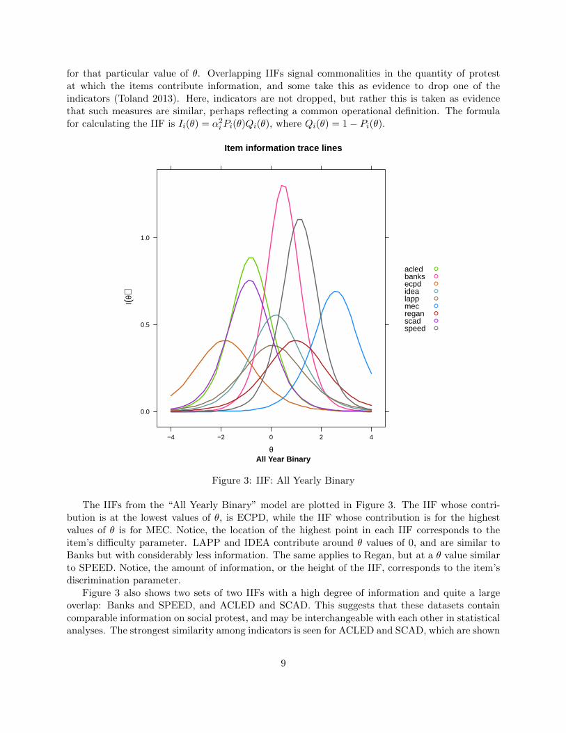
for that particular value of θ. Overlapping IIFs signal commonalities in the quantity of protestat which the items contribute information, and some take this as evidence to drop one of theindicators (Toland 2013). Here, indicators are not dropped, but rather this is taken as evidencethat such measures are similar, perhaps reflecting a common operational definition. The formulafor calculating the IIF is Ii(θ) = α2

iPi(θ)Qi(θ), where Qi(θ) = 1− Pi(θ).

Item information trace lines

All Year Binaryθ

I(θ)

0.0

0.5

1.0

−4 −2 0 2 4

acledbanksecpdidealappmecreganscadspeed

●

●

●

●

●

●

●

●

●

Figure 3: IIF: All Yearly Binary

The IIFs from the “All Yearly Binary” model are plotted in Figure 3. The IIF whose contri-bution is at the lowest values of θ, is ECPD, while the IIF whose contribution is for the highestvalues of θ is for MEC. Notice, the location of the highest point in each IIF corresponds to theitem’s difficulty parameter. LAPP and IDEA contribute around θ values of 0, and are similar toBanks but with considerably less information. The same applies to Regan, but at a θ value similarto SPEED. Notice, the amount of information, or the height of the IIF, corresponds to the item’sdiscrimination parameter.

Figure 3 also shows two sets of two IIFs with a high degree of information and quite a largeoverlap: Banks and SPEED, and ACLED and SCAD. This suggests that these datasets containcomparable information on social protest, and may be interchangeable with each other in statisticalanalyses. The strongest similarity among indicators is seen for ACLED and SCAD, which are shown

9

to contribute for lower values of θ, consistent with their event-based coding schemes. SPEED,however, is also an event-level dataset, and yet its impact on θ is primarily at the higher levels.SPEED and Regan are quite similar as well, albeit with much more information contributed bySPEED.

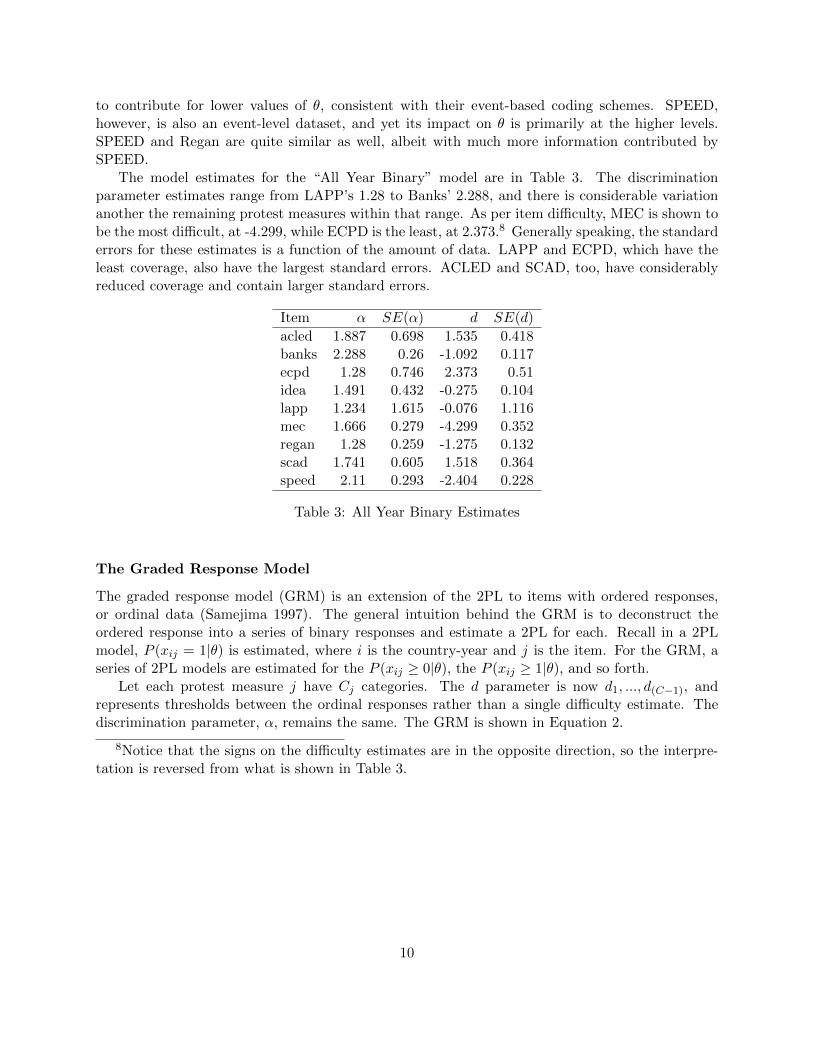
The model estimates for the “All Year Binary” model are in Table 3. The discriminationparameter estimates range from LAPP’s 1.28 to Banks’ 2.288, and there is considerable variationanother the remaining protest measures within that range. As per item difficulty, MEC is shown tobe the most difficult, at -4.299, while ECPD is the least, at 2.373.8 Generally speaking, the standarderrors for these estimates is a function of the amount of data. LAPP and ECPD, which have theleast coverage, also have the largest standard errors. ACLED and SCAD, too, have considerablyreduced coverage and contain larger standard errors.

Item α SE(α) d SE(d)

acled 1.887 0.698 1.535 0.418banks 2.288 0.26 -1.092 0.117ecpd 1.28 0.746 2.373 0.51idea 1.491 0.432 -0.275 0.104lapp 1.234 1.615 -0.076 1.116mec 1.666 0.279 -4.299 0.352regan 1.28 0.259 -1.275 0.132scad 1.741 0.605 1.518 0.364speed 2.11 0.293 -2.404 0.228

Table 3: All Year Binary Estimates

The Graded Response Model

The graded response model (GRM) is an extension of the 2PL to items with ordered responses,or ordinal data (Samejima 1997). The general intuition behind the GRM is to deconstruct theordered response into a series of binary responses and estimate a 2PL for each. Recall in a 2PLmodel, P (xij = 1|θ) is estimated, where i is the country-year and j is the item. For the GRM, aseries of 2PL models are estimated for the P (xij ≥ 0|θ), the P (xij ≥ 1|θ), and so forth.

Let each protest measure j have Cj categories. The d parameter is now d1, ..., d(C−1), andrepresents thresholds between the ordinal responses rather than a single difficulty estimate. Thediscrimination parameter, α, remains the same. The GRM is shown in Equation 2.

8Notice that the signs on the difficulty estimates are in the opposite direction, so the interpre-tation is reversed from what is shown in Table 3.

10

P (xij ≥ 0|θi) = 1

P (xij ≥ 1|θi) =1

1 + exp[−Dα(θi − d1)]

P (xij ≥ 2|θi) =1

1 + exp[−Dα(θi − d2)]

...

P (xij ≥ Cj |θi) = 0 (2)

In the 2PL model, we estimate the probability of a country-year to receive a score of ‘1’ in thedata, given its estimated quantity of protest. In the GRM, we estimate the same probability, butdo so for each level of the ordinal response variable. With respect to the parameters that describethe IRFs, αj , the discrimination parameter, has a similar interpretation to that of the 2PL model.However, instead of a single difficulty parameter, a set of threshold parameters are estimated, equalto the number of categories for a given item minus one. Similar to the difficulty parameter for the2PL model, the threshold estimates are the points at which the slope is the steepest—where thereis a 0.5 probability of observing a category at or below dc.

To estimate the probability of a country-year scoring a certain level of protest (k), we subtractk from k − 1, given θ. For each item, this produces a set of option response functions (ORFs), asshown in Figure 4. Ideally, the ORFs would have steep peaks across values of θ, and their wouldnot be much overlap among them. This would suggest that each protest category is meaningfuland contains information that distinguishes it from other protest categories. In general, this is notobserved.

The ORFs for this model demonstrate that for all indicators, the probability of observing noprotest is high for significant portions of θ. For MEC, the probability of observing no protestis high for nearly the entire range of θ, and never reduces to zero. This is consistent with theinterpretation from the binary model that MEC is a conservative protest measure. The probabilityof observing no protest in the ECPD data, by contrast, reduces to zero at a θ of just above zero,again consistent with the binary model that suggests ECPD is a liberal protest measure. For mostitems, two categories – ‘no protest’ and ‘most protest’ – are the most influential across ORFs, whichis not what would be observed in the ideal case.

There are some examples of steep trace lines with little overlap in Banks, SPEED, and ACELD,but this ideal is neither the case for all levels nor for all indicators. ECPD, for example, showsthat there is considerably high probability of observing categories three through seven for a largerange of θ. This suggests there is not much of a difference in being coded a level ‘3’ or a level‘7.’ However, ECPD also shows that the middle categories are different from the ‘no protest’ and‘most protest’ categories. Examples of less-ideal situations are Regan and SCAD. Here, not only isthere considerable overlap in all categories except for the lowest and highest, but the trace lines areconsiderably flat and represent low densities. This suggests that not only is there little differencein the middle levels of protest, but that changes in the latent quantity of protest have very littleeffect on the probability of observing these levels.

The IIFs of the GRM have a similar interpretation to that of the 2PL, but the appearance isslightly different. Due to the number of threshold estimates, each IIF can potentially contributehigh levels of information across a broad range of θ. An example of this is seen with ECPD, which

11

Item trace lines

All Year Countθ

P(θ

)

0.0

0.2

0.4

0.6

0.8

1.0

−4 −2 0 2 4

acled banks

−4 −2 0 2 4

ecpd

idea lapp

0.0

0.2

0.4

0.6

0.8

1.0

mec

0.0

0.2

0.4

0.6

0.8

1.0

regan

−4 −2 0 2 4

scad speed

cat1cat2cat3cat4cat5cat6cat7cat8cat9

●

●

●

●

●

●

●

●

●

Figure 4: ORF: All Yearly Counts

contributes relatively high degrees of information over the interval of -2 to 2. Overall, however, whilesightly wider than their 2PL counterparts, the IIFs show that the information tends to concentratein small ranges of θ.

As with the 2PL, Banks is the largest contributor of information and is especially influentialat the mid-range values of θ. SPEED overlaps with Banks considerably, and is the second largestcontributor of information. MEC continues to contribute at highest levels of θ, while ACLEDand ECPD are shown to be quite similar, and contain the third and fourth most information,respectively. SCAD, on the other hand, contributes almost no information in this model.

SCAD is perhaps the most detailed and well-documented of all these datasets, so its lack ofinformation is surprising. While this is not a reflection on the validity or reliability of the SCADdata, it is a reflection on its consistency with other protest measures. For example, in both modelsMEC contributes at high values of θ. This means that when protest is observed in the MEC data,it is likely to be observed in the other datasets as well. However, an observed protest in otherdatasets does not necessarily mean it will be observed in MEC. At the count level, SCAD is notconsistent with other protest measures, meaning that increasing (or decreasing) levels in SCAD donot consistently correspond with increasing (or decreasing) levels in other measures.

12

From the data-collection perspective, there are several possibilities as to why this low level ofinformation is observed from SCAD in the count models. One might be that SCAD codes newsreports so closely that it reflects reporting bias more precisely than other indicators. Anotherreason could be that SCAD’s method for distinguishing its start and end dates differ from othermeasures. This may, for example, skew the data towards increased counts for low level proteststhat last for long periods of time. A third reason might be that SCAD is too liberal (in comparisonto others) in its coding of individual protests. That is, where others observe a single protest, SCADpotentially observes many.

Item information trace lines

All Year Countθ

I(θ)

0.0

0.5

1.0

1.5

2.0

−4 −2 0 2 4

acledbanksecpdidealappmecreganscadspeed

●

●

●

●

●

●

●

●

●

Figure 5: IIF: All Yearly Counts

13

Tab

le4:

All

,Y

earl

y,C

ount

Est

imat

es

Item

αSE

(α)

d1

SE

(d1)

d2

SE

(d2)

d3

SE

(d3)

d4

SE

(d4)

d5

SE

(d5)

d6

SE

(d6)

d7

SE

(d7)

d8

SE

(d8)

acl

ed2.2

35

0.4

57

1.7

66

0.3

32

0.0

79

0.2

06

-0.2

95

0.2

07

-0.6

90.2

21

-1.3

58

0.2

72

-2.1

44

0.3

57

-3.3

27

0.4

85

ban

ks

2.5

44

0.4

15

-1.1

71

0.0

31

-3.1

20.2

63

-3.8

70.3

32

-4.4

67

0.3

87

-5.8

13

0.4

91

ecp

d2.1

89

0.3

71

3.0

48

0.3

87

1.6

20.2

78

0.6

30.2

47

-0.1

80.2

6-0

.957

0.2

99

-1.7

85

0.3

59

-2.7

48

0.4

48

-4.0

81

0.5

87

idea

1.9

02

0.1

84

-0.2

88

0.1

11

-1.7

03

0.1

46

-2.1

36

0.1

61

-2.4

44

0.1

71

-3.1

84

0.2

-4.1

17

0.2

46

lap

p1.2

54

1.3

22

-0.0

35

1.0

41

-0.6

37

1.1

42

-0.9

19

1.1

94

-1.2

88

1.2

61

-1.6

86

1.3

43

-2.1

41.4

46

-2.7

04

1.5

78

-3.5

55

1.8

17

mec

1.5

36

0.1

27

-4.1

72

0.1

96

-4.3

34

0.2

02

-4.5

17

0.2

09

-4.7

27

0.2

17

-4.9

81

0.2

28

-6.2

72

0.3

120

-8.0

17

0.6

03

regan

1.4

49

0.1

84

-1.2

97

0.1

28

-1.8

85

0.1

52

-2.2

32

0.1

68

-2.5

37

0.1

83

-2.9

07

0.2

02

-3.3

99

0.2

29

-4.2

22

0.2

83

scad

1.0

70.1

81

1.1

64

0.1

59

0.6

0.1

42

0.2

08

0.1

35

-0.1

95

0.1

33

-0.6

50.1

38

-1.1

14

0.1

48

-1.8

50.1

78

-2.5

07

0.2

23

spee

d2.4

55

0.2

-2.5

98

0.1

71

-4.3

27

0.3

14

-4.8

33

0.3

52

-5.2

68

0.3

82

-6.3

28

0.4

41

14

Table 4 shows the estimates for the “All Year Count” model. For each item, in addition tothe discrimination parameter and its confidence interval, there is also an estimate for thresholdparameters – up to eight are possible – and their associated standard errors. LAPP and SCADhave the lowest ability to discriminate at 1.254 and 1.07, respectively. However, the standard errorfor the LAPP estimate is relatively high (1.322), suggesting more data is necessary to accuratelyestimate the parameters, while SCAD’s standard error is quite low (0.181). This suggests there is ahigh degree of confidence that SCAD is not consistent with other measures. As in the 2PL, Banksdiscriminates best (2.544), although its standard error is slightly larger than most others (0.415).SPEED has the next highest discrimination (2.455), and a lower standard error (0.2).

The threshold estimates take on a slightly different meaning for the GRM, because it is ofinterest to see if and where the categories are valuable. The initial threshold, d1, shows that theseitems have a variety of levels of difficulty – a good sign that the combination of the indicators ismeaningful. The largest changes in the threshold estimates occur at the first and last intervals,suggesting ‘no protest’ and ‘most protest’ are the most distinct levels. Corresponding to decreasingamounts of data, the trend for each item’s standard errors is to increase as the level of protestincreases. This holds for the ‘most protest’ level, and so the analysis of its contribution to themodel should be tempered by the fact that it has the largest standard errors.

Trends in Global Protest: The Value of the Latent Dimension Il-lustrated

Figure 6: Global Reported Events, 1946-2012

Figure 6 illustrates the number of annual reported protests identified by each of the ninedatasets. Because several datasets may report duplicate events, the y-axis should be seen as an

15

Binary Count

Figure 7: Global Protest with Mean IRT, 1946-2012

additive set of protest event counts rather than a raw count of protest events. Nonetheless, as isclear from this figure, with the exception of Banks, MEC, and SPEED most protest datasets do notbegin coverage until 1980. Moreover, some of the datasets with the highest quantity of reportedevents after 1980 have limited geographical and temporal coverage. ECPD, which focuses exclu-sively on Europe, ends coverage in 1995, yielding a sharp decline in the number of reported events.SCADs coverage appears in 1990, yielding a high number of reported events but for Africa only.The difference in spatial and temporal coverage over time illustrates one key challenge in estimatingthe quantity of protest. Another key challenge is the fact that two of the protest databases withthe greatest scope of geographical and temporal coverage (e.g. Banks and SPEED) contribute avery small proportion of the total reported events, suggesting that they significantly underreportevents that other datasets capture.

To illustrate the added value of the IRT exercise, we identify how the binary and count latentmeasures might add information to observed global trends. The left panel of Figure 7 identifies thenumber of datasets with at least one observed protest in a given year – an additive count of binarymeasures of protest. 2005 was the year with the best coverage, since 7 of the 9 datasets identifiedat least one protest in that year. We can see, however, that the mean of our latent binary protestvariable indicates higher levels of potential protest in 1946-1954 than was observed. This is alsotrue in the early-mid 1960s, as well as in 1988-1990 (during the height of the Eastern Europeanrevolutions) and 2011 (the height of the Arab Spring).

These patterns are equally striking when we observe the global reported event counts comparedwith the mean of our latent count variable (right panel of Figure 7 ). Here again, we see a muchhigher latent potential for protest than was observed during the entire 1950-1989 period, and amuch higher latent potential for protest than was reported in 2011.

Returning to the Tunisia case, Figure 8 illustrates the additive event counts from the differentavailable data sets from 1946-2012 (excluding LAPP). Once again, we can see from the left panelFigure 9 that in general, the latent variable for binary protest provides more information than theobserved measures in the 1946-1989 period. Interestingly, the latent measure is quite consistent with

16

Figure 8: Tunisia Reported Events, 1946-2012

the observed binary indicators after 1989. The count variables yield more information, however.From the right panel of Figure 9, we can see that the latent potential for protest is higher thanobserved protest from 1950-2005. Moreover, the latest measure properly categorizes 2010-2012 ashighly contentious years in Tunisian politics.

In summary, both models appear to estimate the latent quantity of protest well, with thecaveat that the GRM is not much more informative than the 2PL, if it is more informative atall. Rather than more accurately reflect a quantity of protest, counts of protest may obscure thatlatent quantity, as is seen in the SCAD example. The test put forth in the following section ismore revealing than a descriptive comparison of the estimates. In the next section, the ability ofthe newly estimated quantity of protest is tested against a well-known forecasting model that hasbeen originally estimated using just the Banks measure.

Authoritarian breakdown

To illustrate one use of the estimated protest data, in this section we present results from author-itarian breakdown models that include this variable as a predictor. The authoritarian breakdowndata are from an updated version of Geddes, Wright and Frantz (2014). The updates include datafrom 1946 to 2012 on 286 autocratic regimes in 119 countries. We examine the post-Cold Warperiod, from 1991-2012, during which 73 autocratic breakdown events occur: 50 democratic tran-sitions and 23 regime breakdown events where the subsequent regime is not a democracy (what wecall autocratic transition). The latter transitions entail one autocratic regime replacing another,

17

Binary Count

Figure 9: Tunisia Protest with Binary IRT Measure, 1946-2012

for example Laurent Kabila’s rebel army ousting the Mobutu regime from Kinshasa in 1997.9

We begin with yearly protest data so that we can examine how well the latent measure per-forms relative to the most widely used extant measure from the Banks data set. First, we testand validate a model using data from 1991-2012 for three dependent variables: all breakdowns,democratic transitions, and autocratic transitions. Below we describe the model specification foreach dependent variable. We estimate a Weibull survival model.10

To validate the model, we conduct out-of-sample tests, following Ward, Greenhill and Bakke(2010). We randomly divide the sample into 10 bins and run the model with data from 9 ofthe 10 bins, using data from the tenth for out-of-sample prediction. We do this ten times, eachtime saving data from a different bin to conduct out-of-sample predictions. We obtain predictionsfrom the survivor function by substracting the bounded predicted survival rate from 1: 1− S. Thisprovides us with one out-of-sample prediction for all data in the sample. We conduct this procedureten times (randomizing differently each time) and average the ten out-of-sample predictions. Wethen calculate the AUC for the averaged out-of-sample predictions, both in a model with the protestinformation and one without them. For each dependent variable, we choose a model specificationwith the highest AUC for these averaged out-of-sample predictions.

Table 5 reports the out-of-sample AUCs for each model (we discuss covariate data and report theestimates for covariates in the Appendix). In each case, we choose a different model specification,including a different protest variable. For example, the All breakdowns model uses a one-year lag

9This latter category also includes regime failures where the subsequent regime is either anoccupying foreign power (e.g. Iraq 2003) or a power vacuum exists such that no internationallyrecognized government controls the majority of territory (e.g. Somalia after the fall of Siad Barrein 1991).

10The hazard rate at time t in this model is h(t,X) = λp(λt)p−1, where λi = eXiβ. X is thevector of explanatory variables and p is a shape parameter that estimates how the hazard changesover time.

18

on the protest measure derived from binary protest data (any vs. none), whereas the Democratictransition model employs the 2-year lagged moving average of the latent protest measure derivedfrom the binary protest data. The set of variables from which we choose are theoretically informed,but the variables specificied in each model, including the protest variable(s), are based on thespecification that yields the highest average AUC score from the out-of-sample validation. For Allbreakdowns and Democratic transitions, adding the protest information from the latent measureincreases the validation AUCs by over 0.02. This means that protest information increases thepredictive accuracy of these models. For the Autocratic transition model, however, adding protestinformation does not change the predictive accuracy of the model.

Table 5: Out-of-sample tests, yearly data

Number AUC w/out AUC withModel of Events Protest Protest Difference

All breakdowns73 0.728 0.765 0.037Latent protest (binary, one-year lag)

Democratic transition50 0.802 0.827 0.025Latent protest (binary, lagged 2-year MA)

Autocratic transition23 0.742 0.743 0.001Latent protest (binary, one-year lag)

1991-2012; 129 regimes in 92 countries.

Figure 10 shows the separation plots for the out-of-sample predictions for the three models inTable 5. While there are some clear misses in the democratic transition separation plot (Azerbaijan1992, Liberia 2003), it performs betterthan the autocratic transitions model, particularly at thehigh end of the instability rank axis.

Table 6: Comparing the Latent and Banks measures, yearly data

Number Banks LatentModel of Events Protest Protest Difference

In-sample AUCs

All breakdowns 73 0.789 0.797 0.008Democratic transition 50 0.849 0.862 0.013Autocratic transition 23 0.788 0.791 0.003

2011-2012 forecast AUCs

All breakdowns 7 0.597 0.605 0.008Democratic transition 6 0.567 0.652 0.085Autocratic transition 1

1991-2012; 129 regimes in 92 countries.

Next we compare each model that uses the latent measure with a similar model that employsthe Banks data. Again, we used out-of-sample validation to choose the Banks protest variable

19

All breakdowns

0

.2

.4

.6

.8

1

Probab

ility of tr

ansition

0 200 400 600 800 1000 1200 1400

Instability rank

Observed transition Predicted probability of transition

Democratic transitions

0

.2

.4

.6

.8

1

Probab

ility of tr

ansition

0 200 400 600 800 1000 1200 1400

Instability rank

Observed transition Predicted probability of transition

Autocratic transitions

0

.2

.4

.6

Probab

ility of tr

ansition

0 200 400 600 800 1000 1200 1400

Instability rank

Observed transition Predicted probability of transition

Figure 10: Separation plots for out-of-sample validation (yearly). Years: 1991-2012. SeeTable 5 details on protest variables.

wth the highest average out-of-sample AUC scores. We also restrict the sample to all observationswith non-missing data on both measures of protest. First, we compare the in-sample AUC scoresfrom models with each of the protest measures. The top panel of Table 6 shows that for eachdependent variable, the latent measure increases the predictive accuracy of the model in-sample,relative to the Banks measure. The relative increase in predictive accuracy, however, is largestfor the Democratic transition model and neglible for the Autocratic transition model. Second, weestimate the model with data from 1991-2010 and gauge the predictive accuracy of the modelagainst observed autocratic breakdowns in the years 2011-12. We only do this for All breakdownsand for Democratic transition because there is only one observation of Autocratic breakdown in thosetwo years. Recall that an AUC score of 0.50 is no better than chance, so overall these forecastsperform poorly relative to the validation and in-sample AUC tests. That said, the forecast using thelatent measure does appreciably better than the forecast using the Banks measure, suggesting somevalue-added to using the latent measure of protest in a predictive model of democratic transition.

Monthly data

A second potential advantage of the latent measure is to utilize the monthly data. Again weexamine a post-Cold War sample (1990-20102) and three dependent variables: All breakdowns,Democratic transitions, and Autocratic transitions.11 During these 23 years here are 80 breakdownevents (56 democratic transitions and 24 autocratic transtions) and over 17,000 non-events months.

11With the yearly data and the one-year lag on the protest variables, the year 1990 was droppedfrom the analysis.

20

We test and validate a model for each dependent variable to maximize the out-of-sample AUCscores, as described above. In addition to the monthly data on protest and regime breakdwon, weutlize monthly data on coups, civil and international conflict, (and elections... not yet!). Data forautocratic regime type and prior democracy vary by regime; and data on infant mortality ratesvary by year. The covariates are: successsful Coup in the past 24 months; Prior democracy; IMRrelative to the world mean; Military regime; Monarchy; Protest; Military × Protest.

For each model (dependent variable, sample) we conducted out-of-sample tests, similar to thoseconducted using the yearly data. The first column of Table 7 reports the average AUC from thesetests without the protest variables, for each of the models (dependent variables). The second columnreports the average out-of-sample AUCs from validation tests with the protest variables, while thethird column shows the difference between the average AUCs in the first and second columns. Whilethe democratic transition models has the best predictive accuracy, including protest informationincreases the out-of-sample AUCs for all the models.

Next we examine the forecast for the months during the calendar years 2011-12. To do this, wetest the model for each dependent variable with data from 1990-2010 and then calculate predictionsfor the months in years 2011-12. We then assess these forecasts with observed monthly data onregime breakdown in 2011-12. The AUCs from these tests are reported in the last column ofTable 7. Again the forecast for democratic transition has a higher AUC than the forecast forall breakdowns, but overall the 2011-12 forecasts are substantially better with the monthly datathan with the yearly data. For example the democratic transition forecast AUC is 0.742 with themonthly data but only 0.652 with the yearly data. Further, the monthly model does not yet havethe monthly election data).

Table 7: Out-of-sample tests, monthly data

Number AUC w/out AUC with ForecastModel of Events Protest Protest Difference AUC

All breakdowns80 0.676 0.744 0.068 0.692Count protest (lagged 4-month MA)

Democratic transition56 0.712 0.788 0.076 0.742Count protest (lagged 6-month MA)

Autocratic transition24 0.542 0.617 0.075Count protest (lagged 2-month MA)

137 regimes in 96 countries from 1990-2012.

It is important to note that the lagged moving averages for protest that yield the best predic-tions are 2-, 4-, and 6-month MAs. This means that moving to monthly data on protests yieldsbetter model predictions than simply using lagged yearly averages for protest, even with data thatmodels these monthly outcome variables. Further, when we test the forecast model for democratictransitions and use the 2-month lagged MA instead of the 6-month lagged MA, the AUC for the2011-12 forecast period is 0.804, which suggests that an even smaller time frame for protest mea-sures may have helped predict autocratic regime breakdown at the monthly level during the 2011-12

21

period.12

Finally, the next iteration of the monthly models will include monthly election data as well astest split population survival models to examine whether structural features (e.g. slowly movinginfant mortality rates) are best modeled that way.

Conclusion

The latent protest variable produced in this analysis performs better in-sample and with models ofdemocratic transition. At this stage, therefore, the added value of this variable is certainly present,although other datasets also perform fairly well overall.

This exercise tells us a few things about current protest databases. First, including protestvariables in models of authoritarian breakdown improves both in-sample and out-of-sample fore-casts of this phenomenon – both in terms of all autocratic breakdown events grouped together anddemocratic transitions. This finding highlights the importance of protest as a covariate and furtherunderscores the necessity of reliable measurement of this indicator. Second, measurement differ-ences across datasets – as modeled by our latent protest indicator – produce nontrivial differencesin the forecasts of different transition types, both in- and out-of-sample. Although the results weresomewhat mixed, where our latent variable performed the best (in terms of democratic transitions),its impact was substantially different from that of different protest databases. As a consequence,our study illustrates the potential value of modeling the latent dimensions of protest rather thansolely relying on observed indicators.

12For all breakdowns, the forecast AUC with a 2-month lag MA is 0.719.

22

References

Baker, Frank B. 2001. The Basics of Item Response Theory. Second ed. New York: ERIC Clear-inghouse.

Baker, Frank B. and Seoch-Ho Kim. 2004. Item Response Theory: Parameter Estimation Tech-niques. Second ed. New York: Marcel Dekker.

Benson, Brett V. and Joshua D. Clinton. 2012. “Measured Strength: Estimating the Strength ofAlliances in the International System, 1881-2000.” Unpublished manuscript.

Chalmers, R. Philip. 2012. “mirt: A Multidimensional Item Response Theory Package for the REnvironment.” Journal of Statistical Software 48(6).

Clinton, Joshua D. and Simon Jackman. 2009. “To Simulate or NOMINATE?” Legislative StudiesQuarterly 24(4):593–621.

D’Orazio, Vito. 2013. International Military Cooperation: From Concepts to Constructs PhD thesisPennsylvania State University.

Geddes, Barbara, Joseph Wright and Erica Frantz. 2014. “Autocratic Regimes: A New Data Set.”Perspectives on Politics 17(1):forthcoming.

Herkenrath, Mark and Alex Knoll. 2011. “Protest events in international press coverage: Anempirical critique of cross-national conflict databases.” International Journal of ComparativeSociology 52(3):163–180.

Hyde, Susan and Nikolay Marinov. 2012. “Which Elections Can Be Lost?” Political Analysis20(2):191–210.

Linden, Wim J. van der and Ronald K. Hambleton. 1997. Item Response Theory: Brief History,Common Models, and Extensions. In Handbook of Modern Item Response Theory, ed. Wim J.van der Linden and Ronald K. Hambleton. Springer New York pp. 1–28.

Marshall, Monty G. and Keith Jaggers. 2007. “Polity IV Project: Political Regime Characteristicsand Transitions 1800–2007.”. Center for Systemic Peace, George Mason University.

McAdam, Doug. 1999. Political process and the development of black insurgency, 1930-1970. Uni-versity of Chicago Press.

Pemstein, Daniel, Stephen A Meserve and James Melton. 2010. “Democratic compromise: A latentvariable analysis of ten measures of regime type.” Political Analysis 18(4):426–449.

Pieroni, Luca, Giorgio d’Agostino and Francesco Bartolucci. 2013. “Identifying corruption throughlatent class models: evidence from transition economies.”.

Powell, Jonathan M and Clayton L Thyne. 2011. “Global instances of coups from 1950 to 2010 Anew dataset.” Journal of Peace Research 48(2):249–259.

Reise, Steven P. and Niels G. Waller. 2009. “Item Response Theory and Clinical Measurement.”Annual Review of Clinical Psychology 5:27–48.

23

Samejima, Fumiko. 1997. Graded Response Model. In Handbook of Modern Item Resonse Theory,ed. Wim J. van der Linden and Ronald K. Lambleton. Springer.

Scott, James C. 1985. Weapons of the weak: Everyday forms of peasant resistance. Yale UniversityPress.

Smith, Jackie, John D McCarthy, Clark McPhail and Boguslaw Augustyn. 2001. “From protestto agenda building: Description bias in media coverage of protest events in Washington, DC.”Social Forces 79(4):1397–1423.

Toland, Michael D. 2013. “Practical Guide to Conducting an Item Response Theory Analysis.”The Journal of Early Adolescence pp. 1–32.

Treier, Shawn and Simon Jackman. 2008. “Democracy as a latent variable.” American Journal ofPolitical Science 52(1):201–217.

Ward, Michael D, Brian D Greenhill and Kristin M Bakke. 2010. “The perils of policy by p-value:Predicting civil conflicts.” Journal of Peace Research 47(4):363–375.

24

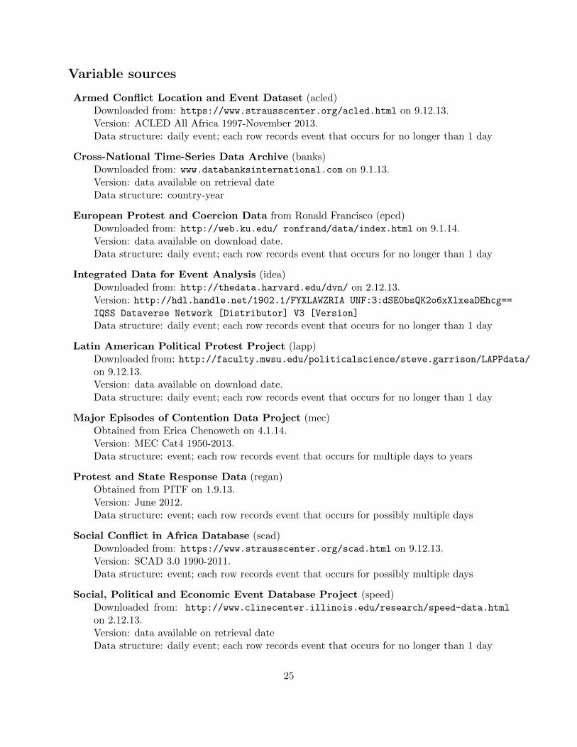
Variable sources

Armed Conflict Location and Event Dataset (acled)Downloaded from: https://www.strausscenter.org/acled.html on 9.12.13.Version: ACLED All Africa 1997-November 2013.Data structure: daily event; each row records event that occurs for no longer than 1 day

Cross-National Time-Series Data Archive (banks)Downloaded from: www.databanksinternational.com on 9.1.13.Version: data available on retrieval dateData structure: country-year

European Protest and Coercion Data from Ronald Francisco (epcd)Downloaded from: http://web.ku.edu/ ronfrand/data/index.html on 9.1.14.Version: data available on download date.Data structure: daily event; each row records event that occurs for no longer than 1 day

Integrated Data for Event Analysis (idea)Downloaded from: http://thedata.harvard.edu/dvn/ on 2.12.13.Version: http://hdl.handle.net/1902.1/FYXLAWZRIA UNF:3:dSE0bsQK2o6xXlxeaDEhcg==

IQSS Dataverse Network [Distributor] V3 [Version]

Data structure: daily event; each row records event that occurs for no longer than 1 day

Latin American Political Protest Project (lapp)Downloaded from: http://faculty.mwsu.edu/politicalscience/steve.garrison/LAPPdata/on 9.12.13.Version: data available on download date.Data structure: daily event; each row records event that occurs for no longer than 1 day

Major Episodes of Contention Data Project (mec)Obtained from Erica Chenoweth on 4.1.14.Version: MEC Cat4 1950-2013.Data structure: event; each row records event that occurs for multiple days to years

Protest and State Response Data (regan)Obtained from PITF on 1.9.13.Version: June 2012.Data structure: event; each row records event that occurs for possibly multiple days

Social Conflict in Africa Database (scad)Downloaded from: https://www.strausscenter.org/scad.html on 9.12.13.Version: SCAD 3.0 1990-2011.Data structure: event; each row records event that occurs for possibly multiple days

Social, Political and Economic Event Database Project (speed)Downloaded from: http://www.clinecenter.illinois.edu/research/speed-data.html

on 2.12.13.Version: data available on retrieval dateData structure: daily event; each row records event that occurs for no longer than 1 day

25

Variable definitions

• acled protest any (binary)Events include: “Riots/Protests” OR [“Non-violent activity by a conflict actor” AND [ “Civil-ians” OR “Protestes” OR “Rioters” as actors]]

Variable values:

0. no protest

1. protest

• acled protest count (count)Events include: “Riots/Protests” OR [“Non-violent activity by a conflict actor” AND [ “Civil-ians” OR “Protestes” OR “Rioters” as actors]]

Variable values:

– number of protests, including zero

• banks protest any (binary)Events include: “Riots” OR “Strikes” OR “Anti-government demonstrations” OR “Non-violent action”

Variable values:

0. no protest

1. protest

• banks protest count (count)Events include: “Riots” OR “Strikes” OR “Anti-government demonstrations” OR “Non-violent action”

Variable values:

– number of protests, including zero

• ecpd protest any (binary)Events include: “accede” OR “adaptation” OR “agreement” OR “ambush” OR “appeal” OR“backlash” OR “battle” OR “blockade” OR “boycott” OR “breakout” OR “break-in” OR“cancel” OR “” OR “censor” OR “ceremony” OR “civil disobedience” OR “closure” OR“commemorate” OR “commitment” OR “compromise” OR “confiscate” OR “confront” OR“conscription” OR “convict” OR “convoy” OR “counter-demonstration/rally” OR “curfew”OR “declare” vOR “defection” OR “defuse” OR “delay” OR “demolish” OR “demonstrate”OR “deploy” OR “deport” OR “destroy” OR “disband” OR “dismiss” OR “disrupt” OR“disolve” OR “disturb” OR “elect” OR “escape” OR “exclude” OR “exit” OR “expel” OR“expulsion” OR “fine” OR “fire” OR “force” OR “funeral” OR “general strike” OR “ha-rass” OR “hide” OR “hunger strike” OR “immolation” OR “impeach” OR “intervention”

26

OR “lockout” OR “mobilize” OR “motorcade” OR “negotiation” OR “obstruct” OR “offer”OR “opposition” OR “oust” OR “petition” OR “preclude” OR “pre-empt” OR “propoganda”OR “proscribe” OR “protest” OR “raid” OR “rally” OR “refuse” OR “reject” OR “release”OR “religion mass” OR “removal” OR “repression” OR “resign” OR “riot” OR “rob” OR“sabotage” OR “satire” OR “search” OR “seize” OR “self-mutilation” OR “shut down” OR“silent protest” OR “sit-in” OR “slowdown” OR “strike” OR “suicide” OR “support” OR“surrender” OR “suspend” OR “symbolic” OR “transfer” OR “trespass” OR “trial” OR “ul-timatim” OR “vigil” OR “vote” OR “walkout” OR “warn” OR “withdraw” OR “with hold”OR “work stoppage”

Variable values:

0. no protest

1. protest

• ecpd protest count (count)Events include: “accede” OR “adaptation” OR “agreement” OR “ambush” OR “appeal” OR“backlash” OR “battle” OR “blockade” OR “boycott” OR “breakout” OR “break-in” OR“cancel” OR “” OR “censor” OR “ceremony” OR “civil disobedience” OR “closure” OR“commemorate” OR “commitment” OR “compromise” OR “confiscate” OR “confront” OR“conscription” OR “convict” OR “convoy” OR “counter-demonstration/rally” OR “curfew”OR “declare” vOR “defection” OR “defuse” OR “delay” OR “demolish” OR “demonstrate”OR “deploy” OR “deport” OR “destroy” OR “disband” OR “dismiss” OR “disrupt” OR“disolve” OR “disturb” OR “elect” OR “escape” OR “exclude” OR “exit” OR “expel” OR“expulsion” OR “fine” OR “fire” OR “force” OR “funeral” OR “general strike” OR “ha-rass” OR “hide” OR “hunger strike” OR “immolation” OR “impeach” OR “intervention”OR “lockout” OR “mobilize” OR “motorcade” OR “negotiation” OR “obstruct” OR “offer”OR “opposition” OR “oust” OR “petition” OR “preclude” OR “pre-empt” OR “propoganda”OR “proscribe” OR “protest” OR “raid” OR “rally” OR “refuse” OR “reject” OR “release”OR “religion mass” OR “removal” OR “repression” OR “resign” OR “riot” OR “rob” OR“sabotage” OR “satire” OR “search” OR “seize” OR “self-mutilation” OR “shut down” OR“silent protest” OR “sit-in” OR “slowdown” OR “strike” OR “suicide” OR “support” OR“surrender” OR “suspend” OR “symbolic” OR “transfer” OR “trespass” OR “trial” OR “ul-timatim” OR “vigil” OR “vote” OR “walkout” OR “warn” OR “withdraw” OR “with hold”OR “work stoppage”

Variable values:

– number of protests, including zero

• idea protest any (binary)Events include: “Non-military demonstrate” (WEISS code 181, civil actor)

Variable values:

0. no protest

27

1. protest

• idea protest count (count)Events include: “Non-military demonstrate” (WEISS code 181, civil actor)Variable values:

– number of protests, including zero

• lapp protest any (binary)Events include:

– Bolivia: “Demonstrations” OR “Protests” OR “Riots” OR “Roadblocks” OR “Sit-ins”OR “Strikes”

– Colombia: “Demonstrations” OR “Protests” OR “Riots” OR “Roadblocks” OR “Sit-ins” OR “Strikes”

– El Salvador: “Demonstrations” OR “March” OR “Occupation” OR “Protests” OR “Ri-ots” OR “Roadblocks” OR “Sit-ins” OR “Strikes”

– Peru: “Demonstrations”

Variable values:

0. no protest

1. protest

• lapp protest count (count)Events include:

– Bolivia: “Demonstrations” OR “Protests” OR “Riots” OR “Roadblocks” OR “Sit-ins”OR “Strikes”

– Colombia: “Demonstrations” OR “Protests” OR “Riots” OR “Roadblocks” OR “Sit-ins” OR “Strikes”

– El Salvador: “Demonstrations” OR “March” OR “Occupation” OR “Protests” OR “Ri-ots” OR “Roadblocks” OR “Sit-ins” OR “Strikes”

– Peru: “Demonstrations”

Variable values:

– number of protests, including zero

• mec protest any (binary)Events include: each calendar day/month/year during which a non-violent protest campaignexisted

Variable values:

0. no protest

1. protest

28

• mec protest count (count)Events include: each calendar day/month/year during which a non-violent protest campaignexisted

Variable values:

– number of protests, including zero

• regan protest any (binary)Events include: each calendar day of protest event. “Protest is a gathering of 50 or morepeople to express a demand for social or political access, tolerance, or resources. A protestaction must be targeted at the state or state policy.” Coded from search terms for “protests”,“riots,” and “demonstrations”

Variable values:

0. no protest

1. protest

• regan protest count (count)Events include: each calendar day of protest event. “Protest is a gathering of 50 or morepeople to express a demand for social or political access, tolerance, or resources. A protestaction must be targeted at the state or state policy.” Coded from search terms for “protests”OR “riots” OR “demonstrations’

Variable values:

– number of protests, including zero

• scad protest any (binary)Events include: “Organized Demonstration” OR “Spontaneous Demonstration” OR “Or-ganized Violent Riot” OR “Spontaneous Violent Riot” OR “General Strike” OR “LimitedStrike”. Coded from search terms for “protest” OR “strike” OR “riot” OR “violence” OR“attack”

Variable values:

0. no protest

1. protest

• scad protest count (count)Events include: “Organized Demonstration” OR “Spontaneous Demonstration” OR “Or-ganized Violent Riot” OR “Spontaneous Violent Riot” OR “General Strike” OR “LimitedStrike”. Coded from search terms for “protest” OR “strike” OR “riot” OR “violence” OR“attack”

Variable values:

29

– number of protests, including zero

• speed protest any (binary)Events include: “Mass demonstrations or strikes” OR “riots or brawls”

Variable values:

0. no protest

1. protest

• speed protest count (count)Events include: “Mass demonstrations or strikes” OR “riots or brawls”

Variable values:

– number of protests, including zero

30

Yearly data

In the Democratic transition model, we employ information from the following variables: a binaryvariable indicating Prior democracy; a binary indicator of a successful Coup in the past four yearsfrom Powell and Thyne (2011); a binary indicator of Military regime from Geddes, Wright andFrantz (2014); a binary indicator of an Incumbent standing in an election either the observation yearor the prior year and an indicator of an international election Monitor present during the electionfrom Hyde and Marinov (2012); and a lagged moving average of the latent Protest constructedfrom count information. The model specification with the highest out-of-sample AUCs from thevalidation also include interaction terms: Mililtary × Protest, Mililtary × Coup, Mililtary ×Incumbent.

In the Autocratic transition model, we employ information from the following variables: a binaryindicator of an attempted Coup in the past year from Powell and Thyne (2011); a binary indicator ofan Irregular election in either the observation year or the prior year from Hyde and Marinov (2012);a continous measure of the infant mortality rate relative to the word mean (IMR); and the 1-yearlag of the latent Protest variable constructed from binary information. The model specificationwith the highest out-of-sample AUCs from the validation test also includes an interaction term:Irregular × Log(duration), where the latter term is the natural log of regime duration in years.

In the All breakdowns model, we employ information from the following variables: a binaryindicator of a successful Coup in the past four years; the 1-year lag of the latent Protest variableconstructed from binary information; Irregular; IMR; Prior; Military; Military × Incumbent; andMilitary × Coup.

31

Table A-1: Authoritarian breakdown, yearly

All Dem Dict

Protest 1.267** 1.182 0.644(0.46) (0.62) (0.67)

Military × Protest -0.860 -1.196(0.88) (1.13)

Military 1.755 2.781*(0.96) (1.24)

Military × Incumbent 1.671** 1.386*(0.59) (0.70)

Military × Coup -3.807 -5.738*(2.41) (2.51)

Coup 5.274** 8.578** -14.493(1.49) (1.61) (16.99)

Prior 0.820** 1.350**(0.30) (0.37)

Incumbent 0.868** 0.781(0.34) (0.45)

Irregular 0.295 7.901**(0.32) (1.79)

IMR 0.550** 0.693**(0.12) (0.19)

Monitor 0.855*(0.43)

Irregular × Log(duration) -2.554**(0.64)

(Intercept) -7.976** -8.027** -11.128**(0.77) (0.90) (1.67)

ln(ρ) 0.268** 0.295** 0.740**(0.10) (0.11) (0.18)

Log likelihood -116.1 -87.9 -55.4Observations 1423 1424 1423

32