A Large Dataset to Train Convolutional Networksfor Disparity, Optical Flow, and Scene Flow Estimation

Nikolaus Mayer∗1, Eddy Ilg∗1, Philip Hausser∗2, Philipp Fischer∗1†1University of Freiburg 2Technical University of Munich

1{mayern,ilg,fischer}@cs.uni-freiburg.de 2haeusser@cs.tum.edu

Daniel CremersTechnical University of Munich

cremers@tum.de

Alexey Dosovitskiy, Thomas BroxUniversity of Freiburg

{dosovits,brox}@cs.uni-freiburg.de

Abstract

Recent work has shown that optical flow estimation canbe formulated as a supervised learning task and can be suc-cessfully solved with convolutional networks. Training ofthe so-called FlowNet was enabled by a large syntheticallygenerated dataset. The present paper extends the conceptof optical flow estimation via convolutional networks to dis-parity and scene flow estimation. To this end, we proposethree synthetic stereo video datasets with sufficient realism,variation, and size to successfully train large networks. Ourdatasets are the first large-scale datasets to enable trainingand evaluating scene flow methods. Besides the datasets,we present a convolutional network for real-time disparityestimation that provides state-of-the-art results. By combin-ing a flow and disparity estimation network and training itjointly, we demonstrate the first scene flow estimation witha convolutional network.

1. IntroductionEstimating scene flow means providing the depth and 3D

motion vectors of all visible points in a stereo video. It isthe “royal league” task when it comes to reconstruction andmotion estimation and provides an important basis for nu-merous higher-level challenges such as advanced driver as-sistance and autonomous systems. Research over the lastdecades has focused on its subtasks, namely disparity esti-mation and optical flow estimation, with considerable suc-cess. The full scene flow problem has not been exploredto the same extent. While partial scene flow can be simplyassembled from the subtask results, it is expected that thejoint estimation of all components would be advantageous,

∗These authors contributed equally†Supported by the Deutsche Telekom Stiftung

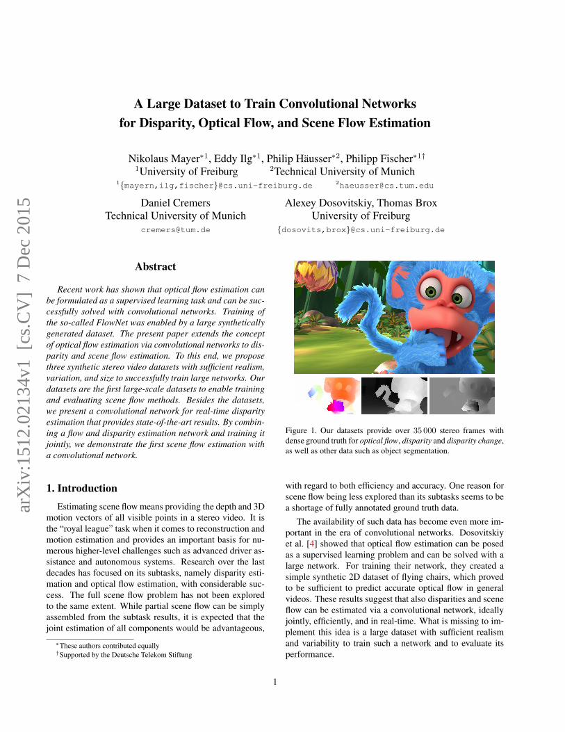
Figure 1. Our datasets provide over 35 000 stereo frames withdense ground truth for optical flow, disparity and disparity change,as well as other data such as object segmentation.

with regard to both efficiency and accuracy. One reason forscene flow being less explored than its subtasks seems to bea shortage of fully annotated ground truth data.

The availability of such data has become even more im-portant in the era of convolutional networks. Dosovitskiyet al. [4] showed that optical flow estimation can be posedas a supervised learning problem and can be solved with alarge network. For training their network, they created asimple synthetic 2D dataset of flying chairs, which provedto be sufficient to predict accurate optical flow in generalvideos. These results suggest that also disparities and sceneflow can be estimated via a convolutional network, ideallyjointly, efficiently, and in real-time. What is missing to im-plement this idea is a large dataset with sufficient realismand variability to train such a network and to evaluate itsperformance.

1

arX

iv:1

512.

0213

4v1

[cs

.CV

] 7

Dec

201

5

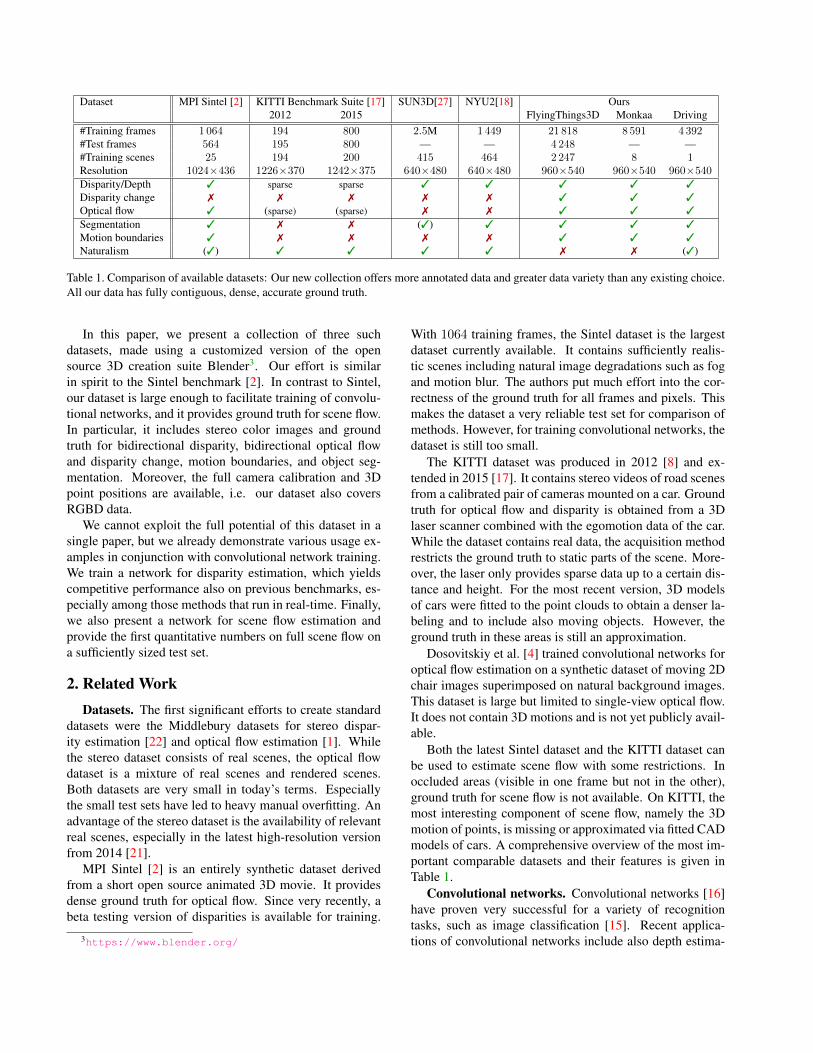
Dataset MPI Sintel [2] KITTI Benchmark Suite [17] SUN3D[27] NYU2[18] Ours2012 2015 FlyingThings3D Monkaa Driving

#Training frames 1 064 194 800 2.5M 1 449 21 818 8 591 4 392#Test frames 564 195 800 — — 4 248 — —#Training scenes 25 194 200 415 464 2 247 8 1Resolution 1024×436 1226×370 1242×375 640×480 640×480 960×540 960×540 960×540Disparity/Depth 3 sparse sparse 3 3 3 3 3Disparity change 7 7 7 7 7 3 3 3Optical flow 3 (sparse) (sparse) 7 7 3 3 3

Segmentation 3 7 7 (3) 3 3 3 3Motion boundaries 3 7 7 7 7 3 3 3Naturalism (3) 3 3 3 3 7 7 (3)

Table 1. Comparison of available datasets: Our new collection offers more annotated data and greater data variety than any existing choice.All our data has fully contiguous, dense, accurate ground truth.

In this paper, we present a collection of three suchdatasets, made using a customized version of the opensource 3D creation suite Blender3. Our effort is similarin spirit to the Sintel benchmark [2]. In contrast to Sintel,our dataset is large enough to facilitate training of convolu-tional networks, and it provides ground truth for scene flow.In particular, it includes stereo color images and groundtruth for bidirectional disparity, bidirectional optical flowand disparity change, motion boundaries, and object seg-mentation. Moreover, the full camera calibration and 3Dpoint positions are available, i.e. our dataset also coversRGBD data.

We cannot exploit the full potential of this dataset in asingle paper, but we already demonstrate various usage ex-amples in conjunction with convolutional network training.We train a network for disparity estimation, which yieldscompetitive performance also on previous benchmarks, es-pecially among those methods that run in real-time. Finally,we also present a network for scene flow estimation andprovide the first quantitative numbers on full scene flow ona sufficiently sized test set.

2. Related WorkDatasets. The first significant efforts to create standard

datasets were the Middlebury datasets for stereo dispar-ity estimation [22] and optical flow estimation [1]. Whilethe stereo dataset consists of real scenes, the optical flowdataset is a mixture of real scenes and rendered scenes.Both datasets are very small in today’s terms. Especiallythe small test sets have led to heavy manual overfitting. Anadvantage of the stereo dataset is the availability of relevantreal scenes, especially in the latest high-resolution versionfrom 2014 [21].

MPI Sintel [2] is an entirely synthetic dataset derivedfrom a short open source animated 3D movie. It providesdense ground truth for optical flow. Since very recently, abeta testing version of disparities is available for training.

3https://www.blender.org/

With 1064 training frames, the Sintel dataset is the largestdataset currently available. It contains sufficiently realis-tic scenes including natural image degradations such as fogand motion blur. The authors put much effort into the cor-rectness of the ground truth for all frames and pixels. Thismakes the dataset a very reliable test set for comparison ofmethods. However, for training convolutional networks, thedataset is still too small.

The KITTI dataset was produced in 2012 [8] and ex-tended in 2015 [17]. It contains stereo videos of road scenesfrom a calibrated pair of cameras mounted on a car. Groundtruth for optical flow and disparity is obtained from a 3Dlaser scanner combined with the egomotion data of the car.While the dataset contains real data, the acquisition methodrestricts the ground truth to static parts of the scene. More-over, the laser only provides sparse data up to a certain dis-tance and height. For the most recent version, 3D modelsof cars were fitted to the point clouds to obtain a denser la-beling and to include also moving objects. However, theground truth in these areas is still an approximation.

Dosovitskiy et al. [4] trained convolutional networks foroptical flow estimation on a synthetic dataset of moving 2Dchair images superimposed on natural background images.This dataset is large but limited to single-view optical flow.It does not contain 3D motions and is not yet publicly avail-able.

Both the latest Sintel dataset and the KITTI dataset canbe used to estimate scene flow with some restrictions. Inoccluded areas (visible in one frame but not in the other),ground truth for scene flow is not available. On KITTI, themost interesting component of scene flow, namely the 3Dmotion of points, is missing or approximated via fitted CADmodels of cars. A comprehensive overview of the most im-portant comparable datasets and their features is given inTable 1.

Convolutional networks. Convolutional networks [16]have proven very successful for a variety of recognitiontasks, such as image classification [15]. Recent applica-tions of convolutional networks include also depth estima-

tion from single images [6], stereo matching [28], and opti-cal flow estimation [4].

The FlowNet of Dosovitskiy et al. [4] is most related toour work. It uses an encoder-decoder architecture with ad-ditional crosslinks between contracting and expanding net-work parts, where the encoder computes abstract featuresfrom receptive fields of increasing size, and the decoderreestablishes the original resolution via an expanding up-convolutional architecture [5]. We adapt this approach fordisparity estimation.

The disparity estimation method in Zbontar et al. [28]uses a Siamese network for computing matching distancesbetween image patches. To actually estimate the disparity,the authors then perform cross-based cost aggregation [29]and semi-global matching (SGM) [11]. In contrast to ourwork, Zbontar et al. have no end-to-end training of a convo-lutional network on the disparity estimation task, with cor-responding consequences for computational efficiency andelegance.

Scene flow. While there are hundreds of papers on dis-parity estimation and optical flow estimation, there are onlya few on scene flow. None of them uses a learning approach.

Scene flow estimation was popularized for the first timeby the work of Vedula et al. [23] who analyzed differentpossible problem settings. Later works were dominated byvariational methods. Huguet and Devernay [12] formulatedscene flow estimation in a joint variational approach. Wedelet al. [26] followed the variational framework but decoupledthe disparity estimation for larger efficiency and accuracy.Vogel et al. [25] combined the task of scene flow estimationwith superpixel segmentation using a piecewise rigid modelfor regularization. Quiroga et al. [19] extended the regular-izer further to a smooth field of rigid motion. Like Wedelet al. [26] they decoupled the disparity estimation and re-placed it by the depth values of RGBD videos.

The fastest method in KITTI’s scene flow top 7 is fromCech et al. [3] with a runtime of 2.4 seconds. The methodemploys a seed growing algorithm for simultaneous dispar-ity and optical flow estimation.

3. Definition of Scene FlowOptical flow is a projection of the world’s 3D motion

onto the image plane. Commonly, scene flow is consid-ered as the underlying 3D motion field that can be computedfrom stereo videos or RGBD videos. Assume two succes-sive time frames t and t+1 of a stereo pair, yielding fourimages (ItL, ItR, It+1

L , It+1R ). Scene flow provides for each

visible point in one of these four images the point’s 3D po-sition and its 3D motion vector [24].

These 3D quantities can be computed only in the caseof known camera intrinsics and extrinsics. A camera-independent definition of scene flow is obtained by the sep-arate components optical flow, the disparity, and the dispar-

Left:

Right:

t-1 t t+1Forward

Flow

Backward

Flow

Disp

.

Disp

.Disp. Ch.Disp. Ch.

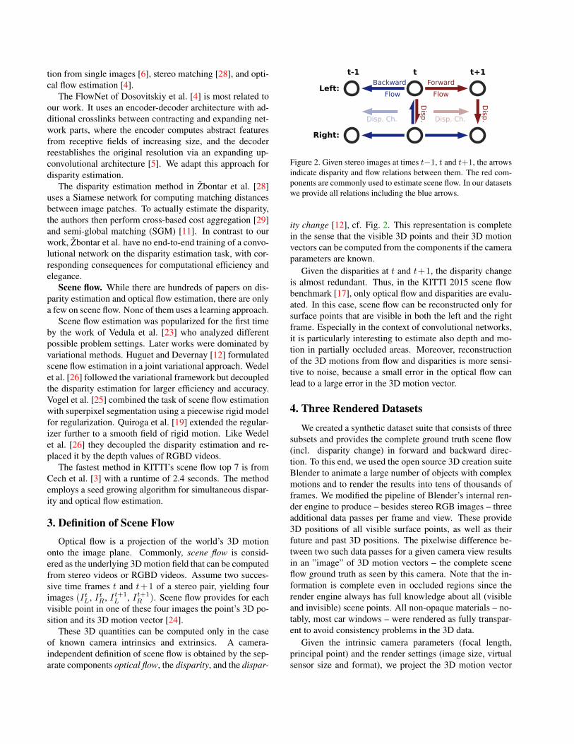
Figure 2. Given stereo images at times t−1, t and t+1, the arrowsindicate disparity and flow relations between them. The red com-ponents are commonly used to estimate scene flow. In our datasetswe provide all relations including the blue arrows.

ity change [12], cf. Fig. 2. This representation is completein the sense that the visible 3D points and their 3D motionvectors can be computed from the components if the cameraparameters are known.

Given the disparities at t and t+1, the disparity changeis almost redundant. Thus, in the KITTI 2015 scene flowbenchmark [17], only optical flow and disparities are evalu-ated. In this case, scene flow can be reconstructed only forsurface points that are visible in both the left and the rightframe. Especially in the context of convolutional networks,it is particularly interesting to estimate also depth and mo-tion in partially occluded areas. Moreover, reconstructionof the 3D motions from flow and disparities is more sensi-tive to noise, because a small error in the optical flow canlead to a large error in the 3D motion vector.

4. Three Rendered Datasets

We created a synthetic dataset suite that consists of threesubsets and provides the complete ground truth scene flow(incl. disparity change) in forward and backward direc-tion. To this end, we used the open source 3D creation suiteBlender to animate a large number of objects with complexmotions and to render the results into tens of thousands offrames. We modified the pipeline of Blender’s internal ren-der engine to produce – besides stereo RGB images – threeadditional data passes per frame and view. These provide3D positions of all visible surface points, as well as theirfuture and past 3D positions. The pixelwise difference be-tween two such data passes for a given camera view resultsin an ”image” of 3D motion vectors – the complete sceneflow ground truth as seen by this camera. Note that the in-formation is complete even in occluded regions since therender engine always has full knowledge about all (visibleand invisible) scene points. All non-opaque materials – no-tably, most car windows – were rendered as fully transpar-ent to avoid consistency problems in the 3D data.

Given the intrinsic camera parameters (focal length,principal point) and the render settings (image size, virtualsensor size and format), we project the 3D motion vector

of each pixel into a 2D pixel motion vector coplanar to theimaging plane: the optical flow. Depth is directly retrievedfrom a pixel’s 3D position and converted to disparity usingthe known configuration of the virtual stereo rig. We com-pute the disparity change from the depth component of the3D motion vector. An example of the results is shown inFig. 1.

In addition, we rendered object segmentation masks inwhich each pixel’s value corresponds to the unique indexof its object. Objects can consist of multiple subparts, ofwhich each can have a separate material (with own appear-ance properties such as textures). We make use of this andrender additional segmentation masks, where each pixel en-codes its material’s index. The recently available beta ver-sion of Sintel also includes this data.

Similar to the Sintel dataset, we also provide motionboundaries which highlight pixels between at least twomoving objects, if the following holds: The difference inmotion between the two frames is at least 1.5 pixels, andthe boundary segment covers an area of at least 10 pixels.The thresholds were chosen to match the results of Sintel’ssegmentation.

For all frames and views, we provide the full cameraintrinsics and extrinsics matrices. Those can be used forstructure from motion or other tasks that require cameratracking. We rendered all image data using a virtual focallength of 35mm on a 32mm wide simulated sensor. For theDriving dataset we added a wide-angle version using a fo-cal length of 15mm which is visually closer to the existingKITTI datasets.

Like the Sintel dataset, our datasets also include two dis-tinct versions of every image: the clean pass shows col-ors, textures and scene lighting but no image degradations,while the final pass additionally includes postprocessing ef-fects such as simulated depth-of-field blur, motion blur, sun-light glare, and gamma curve manipulation.

To handle the massive amount of data (2.5 TB), we com-pressed all RGB image data to the lossy but high-qualityWebP4 format. Non-RGB data was compressed losslesslyusing LZO5.

4.1. FlyingThings3D

The main part of the new data collection consists ofeveryday objects flying along randomized 3D trajectories.We generated about 25 000 stereo frames with ground truthdata. Instead of focusing on a particular task (like KITTI) orenforcing strict naturalism (like Sintel), we rely on random-ness and a large pool of rendering assets to generate ordersof magnitude more data than any existing option, withoutrunning a risk of repetition or saturation. Data generation isfast, fully automatic, and yields dense accurate ground truth

4https://developers.google.com/speed/webp/5http://www.oberhumer.com/opensource/lzo/

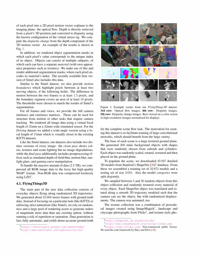
Figure 3. Example scenes from our FlyingThings3D dataset.3rd row: Optical flow images, 4th row: Disparity images,5th row: Disparity change images. Best viewed on a color screenin high resolution (images normalized for display).

for the complete scene flow task. The motivation for creat-ing this dataset is to facilitate training of large convolutionalnetworks, which should benefit from the large variety.

The base of each scene is a large textured ground plane.We generated 200 static background objects with shapesthat were randomly chosen from cuboids and cylinders.Each object was randomly scaled, rotated, textured and thenplaced on the ground plane.

To populate the scene, we downloaded 35 927 detailed3D models from Stanford’s ShapeNet [20]6 database. Fromthese we assembled a training set of 32 872 models and atesting set of size 3 055. Also the model categories weresplit disjointly.

We sampled between 5 and 20 random objects from thisobject collection and randomly textured every material ofevery object. Each ShapeNet object was translated and ro-tated along a smooth 3D trajectory modeled such that thecamera can see the object, but with randomized displace-ments. The camera was animated, too.

The texture collection was a combination of procedu-ral images created using ImageMagick7, landscape andcityscape photographs from Flickr8, and texture-style pho-

6http://shapenet.cs.stanford.edu/7http://www.imagemagick.org/script/index.php8https://www.flickr.com/ Non-commercial public license.

We used the code framework by Hays and Efros [10]

KITTI 2015 Driving (ours)

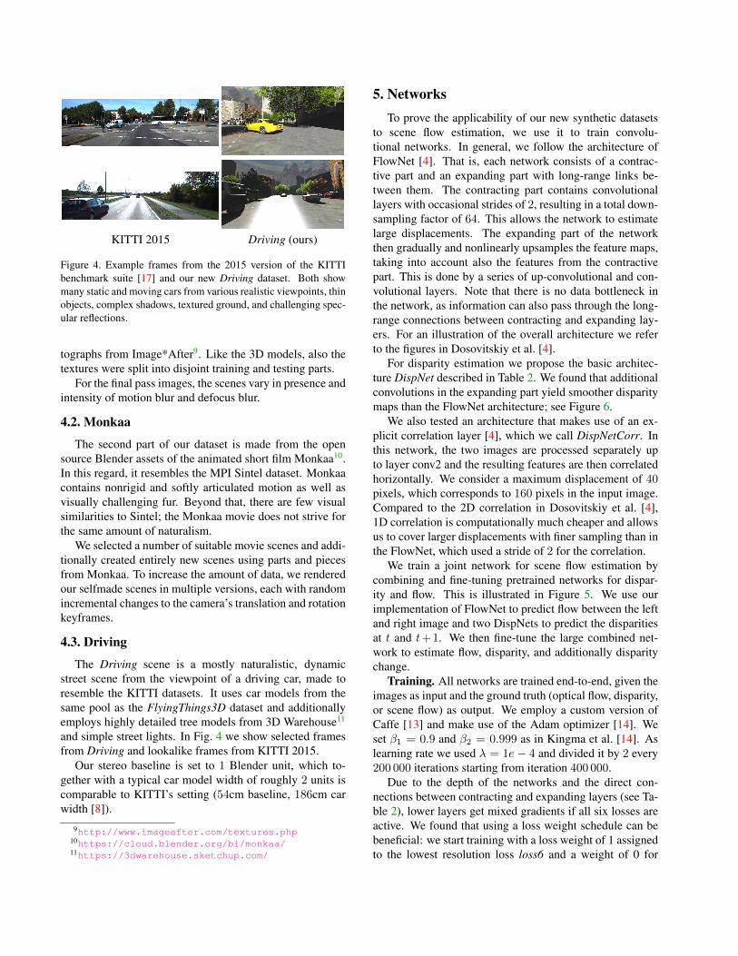
Figure 4. Example frames from the 2015 version of the KITTIbenchmark suite [17] and our new Driving dataset. Both showmany static and moving cars from various realistic viewpoints, thinobjects, complex shadows, textured ground, and challenging spec-ular reflections.

tographs from Image*After9. Like the 3D models, also thetextures were split into disjoint training and testing parts.

For the final pass images, the scenes vary in presence andintensity of motion blur and defocus blur.

4.2. Monkaa

The second part of our dataset is made from the opensource Blender assets of the animated short film Monkaa10.In this regard, it resembles the MPI Sintel dataset. Monkaacontains nonrigid and softly articulated motion as well asvisually challenging fur. Beyond that, there are few visualsimilarities to Sintel; the Monkaa movie does not strive forthe same amount of naturalism.

We selected a number of suitable movie scenes and addi-tionally created entirely new scenes using parts and piecesfrom Monkaa. To increase the amount of data, we renderedour selfmade scenes in multiple versions, each with randomincremental changes to the camera’s translation and rotationkeyframes.

4.3. Driving

The Driving scene is a mostly naturalistic, dynamicstreet scene from the viewpoint of a driving car, made toresemble the KITTI datasets. It uses car models from thesame pool as the FlyingThings3D dataset and additionallyemploys highly detailed tree models from 3D Warehouse11

and simple street lights. In Fig. 4 we show selected framesfrom Driving and lookalike frames from KITTI 2015.

Our stereo baseline is set to 1 Blender unit, which to-gether with a typical car model width of roughly 2 units iscomparable to KITTI’s setting (54cm baseline, 186cm carwidth [8]).

9http://www.imageafter.com/textures.php10https://cloud.blender.org/bi/monkaa/11https://3dwarehouse.sketchup.com/

5. NetworksTo prove the applicability of our new synthetic datasets

to scene flow estimation, we use it to train convolu-tional networks. In general, we follow the architecture ofFlowNet [4]. That is, each network consists of a contrac-tive part and an expanding part with long-range links be-tween them. The contracting part contains convolutionallayers with occasional strides of 2, resulting in a total down-sampling factor of 64. This allows the network to estimatelarge displacements. The expanding part of the networkthen gradually and nonlinearly upsamples the feature maps,taking into account also the features from the contractivepart. This is done by a series of up-convolutional and con-volutional layers. Note that there is no data bottleneck inthe network, as information can also pass through the long-range connections between contracting and expanding lay-ers. For an illustration of the overall architecture we referto the figures in Dosovitskiy et al. [4].

For disparity estimation we propose the basic architec-ture DispNet described in Table 2. We found that additionalconvolutions in the expanding part yield smoother disparitymaps than the FlowNet architecture; see Figure 6.

We also tested an architecture that makes use of an ex-plicit correlation layer [4], which we call DispNetCorr. Inthis network, the two images are processed separately upto layer conv2 and the resulting features are then correlatedhorizontally. We consider a maximum displacement of 40pixels, which corresponds to 160 pixels in the input image.Compared to the 2D correlation in Dosovitskiy et al. [4],1D correlation is computationally much cheaper and allowsus to cover larger displacements with finer sampling than inthe FlowNet, which used a stride of 2 for the correlation.

We train a joint network for scene flow estimation bycombining and fine-tuning pretrained networks for dispar-ity and flow. This is illustrated in Figure 5. We use ourimplementation of FlowNet to predict flow between the leftand right image and two DispNets to predict the disparitiesat t and t+1. We then fine-tune the large combined net-work to estimate flow, disparity, and additionally disparitychange.

Training. All networks are trained end-to-end, given theimages as input and the ground truth (optical flow, disparity,or scene flow) as output. We employ a custom version ofCaffe [13] and make use of the Adam optimizer [14]. Weset β1 = 0.9 and β2 = 0.999 as in Kingma et al. [14]. Aslearning rate we used λ = 1e− 4 and divided it by 2 every200 000 iterations starting from iteration 400 000.

Due to the depth of the networks and the direct con-nections between contracting and expanding layers (see Ta-ble 2), lower layers get mixed gradients if all six losses areactive. We found that using a loss weight schedule can bebeneficial: we start training with a loss weight of 1 assignedto the lowest resolution loss loss6 and a weight of 0 for

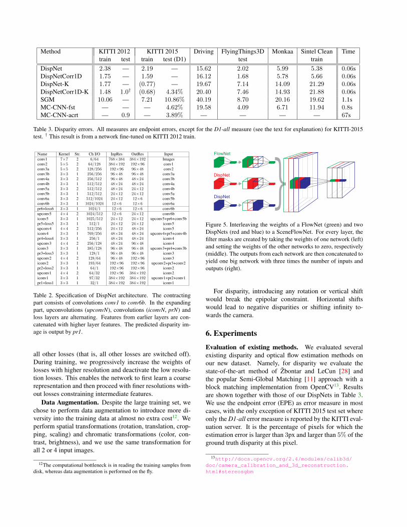
Method KITTI 2012 KITTI 2015 Driving FlyingThings3D Monkaa Sintel Clean Timetrain test train test (D1) test train

DispNet 2.38 — 2.19 — 15.62 2.02 5.99 5.38 0.06sDispNetCorr1D 1.75 — 1.59 — 16.12 1.68 5.78 5.66 0.06sDispNet-K 1.77 — (0.77) — 19.67 7.14 14.09 21.29 0.06sDispNetCorr1D-K 1.48 1.0† (0.68) 4.34% 20.40 7.46 14.93 21.88 0.06sSGM 10.06 — 7.21 10.86% 40.19 8.70 20.16 19.62 1.1sMC-CNN-fst — — — 4.62% 19.58 4.09 6.71 11.94 0.8sMC-CNN-acrt — 0.9 — 3.89% — — — — 67s

Table 3. Disparity errors. All measures are endpoint errors, except for the D1-all measure (see the text for explanation) for KITTI-2015test. † This result is from a network fine-tuned on KITTI 2012 train.

Name Kernel Str. Ch I/O InpRes OutRes Inputconv1 7×7 2 6/64 768×384 384×192 Imagesconv2 5×5 2 64/128 384×192 192×96 conv1conv3a 5×5 2 128/256 192×96 96×48 conv2conv3b 3×3 1 256/256 96×48 96×48 conv3aconv4a 3×3 2 256/512 96×48 48×24 conv3bconv4b 3×3 1 512/512 48×24 48×24 conv4aconv5a 3×3 2 512/512 48×24 24×12 conv4bconv5b 3×3 1 512/512 24×12 24×12 conv5aconv6a 3×3 2 512/1024 24×12 12×6 conv5bconv6b 3×3 1 1024/1024 12×6 12×6 conv6apr6+loss6 3×3 1 1024/1 12×6 12×6 conv6bupconv5 4×4 2 1024/512 12×6 24×12 conv6biconv5 3×3 1 1025/512 24×12 24×12 upconv5+pr6+conv5bpr5+loss5 3×3 1 512/1 24×12 24×12 iconv5upconv4 4×4 2 512/256 24×12 48×24 iconv5iconv4 3×3 1 769/256 48×24 48×24 upconv4+pr5+conv4bpr4+loss4 3×3 1 256/1 48×24 48×24 iconv4upconv3 4×4 2 256/128 48×24 96×48 iconv4iconv3 3×3 1 385/128 96×48 96×48 upconv3+pr4+conv3bpr3+loss3 3×3 1 128/1 96×48 96×48 iconv3upconv2 4×4 2 128/64 96×48 192×96 iconv3iconv2 3×3 1 193/64 192×96 192×96 upconv2+pr3+conv2pr2+loss2 3×3 1 64/1 192×96 192×96 iconv2upconv1 4×4 2 64/32 192×96 384×192 iconv2iconv1 3×3 1 97/32 384×192 384×192 upconv1+pr2+conv1pr1+loss1 3×3 1 32/1 384×192 384×192 iconv1

Table 2. Specification of DispNet architecture. The contractingpart consists of convolutions conv1 to conv6b. In the expandingpart, upconvolutions (upconvN), convolutions (iconvN, prN) andloss layers are alternating. Features from earlier layers are con-catenated with higher layer features. The predicted disparity im-age is output by pr1.

all other losses (that is, all other losses are switched off).During training, we progressively increase the weights oflosses with higher resolution and deactivate the low resolu-tion losses. This enables the network to first learn a coarserepresentation and then proceed with finer resolutions with-out losses constraining intermediate features.

Data Augmentation. Despite the large training set, wechose to perform data augmentation to introduce more di-versity into the training data at almost no extra cost12. Weperform spatial transformations (rotation, translation, crop-ping, scaling) and chromatic transformations (color, con-trast, brightness), and we use the same transformation forall 2 or 4 input images.

12The computational bottleneck is in reading the training samples fromdisk, whereas data augmentation is performed on the fly.

}FlowNet

DispNet

DispNet

Figure 5. Interleaving the weights of a FlowNet (green) and twoDispNets (red and blue) to a SceneFlowNet. For every layer, thefilter masks are created by taking the weights of one network (left)and setting the weights of the other networks to zero, respectively(middle). The outputs from each network are then concatenated toyield one big network with three times the number of inputs andoutputs (right).

For disparity, introducing any rotation or vertical shiftwould break the epipolar constraint. Horizontal shiftswould lead to negative disparities or shifting infinity to-wards the camera.

6. Experiments

Evaluation of existing methods. We evaluated severalexisting disparity and optical flow estimation methods onour new dataset. Namely, for disparity we evaluate thestate-of-the-art method of Zbontar and LeCun [28] andthe popular Semi-Global Matching [11] approach with ablock matching implementation from OpenCV13. Resultsare shown together with those of our DispNets in Table 3.We use the endpoint error (EPE) as error measure in mostcases, with the only exception of KITTI 2015 test set whereonly the D1-all error measure is reported by the KITTI eval-uation server. It is the percentage of pixels for which theestimation error is larger than 3px and larger than 5% of theground truth disparity at this pixel.

13http://docs.opencv.org/2.4/modules/calib3d/doc/camera_calibration_and_3d_reconstruction.html#stereosgbm

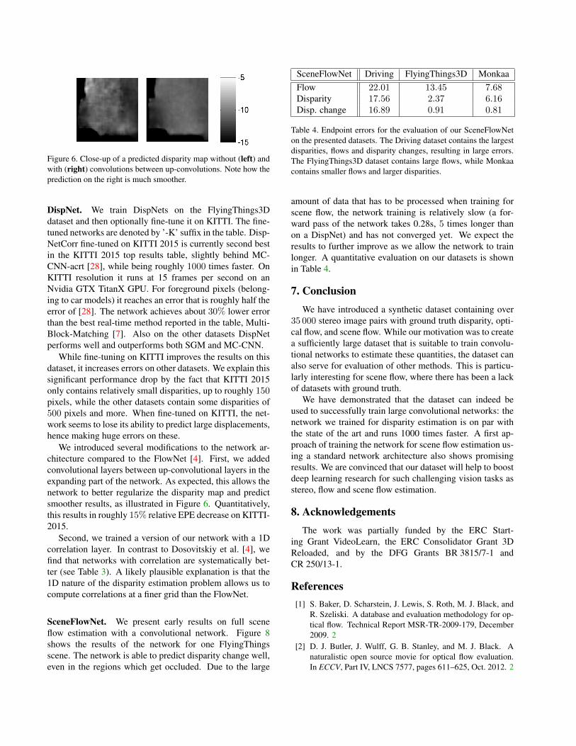
Figure 6. Close-up of a predicted disparity map without (left) andwith (right) convolutions between up-convolutions. Note how theprediction on the right is much smoother.

DispNet. We train DispNets on the FlyingThings3Ddataset and then optionally fine-tune it on KITTI. The fine-tuned networks are denoted by ’-K’ suffix in the table. Disp-NetCorr fine-tuned on KITTI 2015 is currently second bestin the KITTI 2015 top results table, slightly behind MC-CNN-acrt [28], while being roughly 1000 times faster. OnKITTI resolution it runs at 15 frames per second on anNvidia GTX TitanX GPU. For foreground pixels (belong-ing to car models) it reaches an error that is roughly half theerror of [28]. The network achieves about 30% lower errorthan the best real-time method reported in the table, Multi-Block-Matching [7]. Also on the other datasets DispNetperforms well and outperforms both SGM and MC-CNN.

While fine-tuning on KITTI improves the results on thisdataset, it increases errors on other datasets. We explain thissignificant performance drop by the fact that KITTI 2015only contains relatively small disparities, up to roughly 150pixels, while the other datasets contain some disparities of500 pixels and more. When fine-tuned on KITTI, the net-work seems to lose its ability to predict large displacements,hence making huge errors on these.

We introduced several modifications to the network ar-chitecture compared to the FlowNet [4]. First, we addedconvolutional layers between up-convolutional layers in theexpanding part of the network. As expected, this allows thenetwork to better regularize the disparity map and predictsmoother results, as illustrated in Figure 6. Quantitatively,this results in roughly 15% relative EPE decrease on KITTI-2015.

Second, we trained a version of our network with a 1Dcorrelation layer. In contrast to Dosovitskiy et al. [4], wefind that networks with correlation are systematically bet-ter (see Table 3). A likely plausible explanation is that the1D nature of the disparity estimation problem allows us tocompute correlations at a finer grid than the FlowNet.

SceneFlowNet. We present early results on full sceneflow estimation with a convolutional network. Figure 8shows the results of the network for one FlyingThingsscene. The network is able to predict disparity change well,even in the regions which get occluded. Due to the large

SceneFlowNet Driving FlyingThings3D MonkaaFlow 22.01 13.45 7.68Disparity 17.56 2.37 6.16Disp. change 16.89 0.91 0.81

Table 4. Endpoint errors for the evaluation of our SceneFlowNeton the presented datasets. The Driving dataset contains the largestdisparities, flows and disparity changes, resulting in large errors.The FlyingThings3D dataset contains large flows, while Monkaacontains smaller flows and larger disparities.

amount of data that has to be processed when training forscene flow, the network training is relatively slow (a for-ward pass of the network takes 0.28s, 5 times longer thanon a DispNet) and has not converged yet. We expect theresults to further improve as we allow the network to trainlonger. A quantitative evaluation on our datasets is shownin Table 4.

7. ConclusionWe have introduced a synthetic dataset containing over

35 000 stereo image pairs with ground truth disparity, opti-cal flow, and scene flow. While our motivation was to createa sufficiently large dataset that is suitable to train convolu-tional networks to estimate these quantities, the dataset canalso serve for evaluation of other methods. This is particu-larly interesting for scene flow, where there has been a lackof datasets with ground truth.

We have demonstrated that the dataset can indeed beused to successfully train large convolutional networks: thenetwork we trained for disparity estimation is on par withthe state of the art and runs 1000 times faster. A first ap-proach of training the network for scene flow estimation us-ing a standard network architecture also shows promisingresults. We are convinced that our dataset will help to boostdeep learning research for such challenging vision tasks asstereo, flow and scene flow estimation.

8. AcknowledgementsThe work was partially funded by the ERC Start-

ing Grant VideoLearn, the ERC Consolidator Grant 3DReloaded, and by the DFG Grants BR 3815/7-1 andCR 250/13-1.

References[1] S. Baker, D. Scharstein, J. Lewis, S. Roth, M. J. Black, and

R. Szeliski. A database and evaluation methodology for op-tical flow. Technical Report MSR-TR-2009-179, December2009. 2

[2] D. J. Butler, J. Wulff, G. B. Stanley, and M. J. Black. Anaturalistic open source movie for optical flow evaluation.In ECCV, Part IV, LNCS 7577, pages 611–625, Oct. 2012. 2

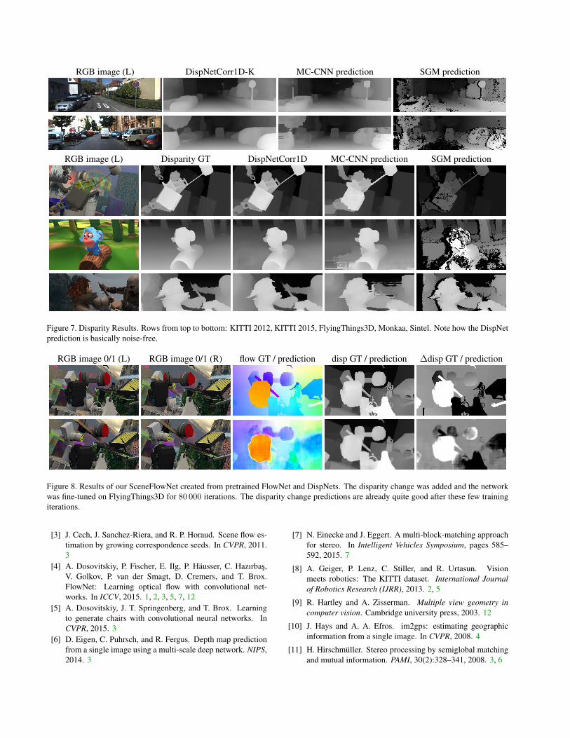
RGB image (L) DispNetCorr1D-K MC-CNN prediction SGM prediction

RGB image (L) Disparity GT DispNetCorr1D MC-CNN prediction SGM prediction

Figure 7. Disparity Results. Rows from top to bottom: KITTI 2012, KITTI 2015, FlyingThings3D, Monkaa, Sintel. Note how the DispNetprediction is basically noise-free.

RGB image 0/1 (L) RGB image 0/1 (R) flow GT / prediction disp GT / prediction ∆disp GT / prediction

Figure 8. Results of our SceneFlowNet created from pretrained FlowNet and DispNets. The disparity change was added and the networkwas fine-tuned on FlyingThings3D for 80 000 iterations. The disparity change predictions are already quite good after these few trainingiterations.

[3] J. Cech, J. Sanchez-Riera, and R. P. Horaud. Scene flow es-timation by growing correspondence seeds. In CVPR, 2011.3

[4] A. Dosovitskiy, P. Fischer, E. Ilg, P. Hausser, C. Hazırbas,V. Golkov, P. van der Smagt, D. Cremers, and T. Brox.FlowNet: Learning optical flow with convolutional net-works. In ICCV, 2015. 1, 2, 3, 5, 7, 12

[5] A. Dosovitskiy, J. T. Springenberg, and T. Brox. Learningto generate chairs with convolutional neural networks. InCVPR, 2015. 3

[6] D. Eigen, C. Puhrsch, and R. Fergus. Depth map predictionfrom a single image using a multi-scale deep network. NIPS,2014. 3

[7] N. Einecke and J. Eggert. A multi-block-matching approachfor stereo. In Intelligent Vehicles Symposium, pages 585–592, 2015. 7

[8] A. Geiger, P. Lenz, C. Stiller, and R. Urtasun. Visionmeets robotics: The KITTI dataset. International Journalof Robotics Research (IJRR), 2013. 2, 5

[9] R. Hartley and A. Zisserman. Multiple view geometry incomputer vision. Cambridge university press, 2003. 12

[10] J. Hays and A. A. Efros. im2gps: estimating geographicinformation from a single image. In CVPR, 2008. 4

[11] H. Hirschmuller. Stereo processing by semiglobal matchingand mutual information. PAMI, 30(2):328–341, 2008. 3, 6

[12] F. Huguet and F. Deverney. A variational method for sceneflow estimation from stereo sequences. In ICCV, 2007. 3

[13] Y. Jia, E. Shelhamer, J. Donahue, S. Karayev, J. Long, R. Gir-shick, S. Guadarrama, and T. Darrell. Caffe: Convolu-tional architecture for fast feature embedding. arXiv preprintarXiv:1408.5093, 2014. 5

[14] D. P. Kingma and J. Ba. Adam: A method for stochasticoptimization. In ICLR, 2015. 5

[15] A. Krizhevsky, I. Sutskever, and G. E. Hinton. Imagenetclassification with deep convolutional neural networks. InNIPS, pages 1106–1114, 2012. 2

[16] Y. LeCun, B. Boser, J. S. Denker, D. Henderson, R. E.Howard, W. Hubbard, and L. D. Jackel. Backpropagationapplied to handwritten zip code recognition. Neural compu-tation, 1(4):541–551, 1989. 2

[17] M. Menze and A. Geiger. Object scene flow for autonomousvehicles. In Conference on Computer Vision and PatternRecognition (CVPR), 2015. 2, 3, 5

[18] P. K. Nathan Silberman, Derek Hoiem and R. Fergus. Indoorsegmentation and support inference from rgbd images. InECCV, 2012. 2

[19] J. Quiroga, F. Devernay, and J. Crowley. Scene flow bytracking in intensity and depth data. In Computer Vision andPattern Recognition Workshops (CVPRW), 2012 IEEE Com-puter Society Conference on, pages 50–57. IEEE, 2012. 3

[20] M. Savva, A. X. Chang, and P. Hanrahan. Semantically-Enriched 3D Models for Common-sense Knowledge. CVPR2015 Workshop on Functionality, Physics, Intentionality andCausality, 2015. 4

[21] D. Scharstein, H. Hirschmuller, Y. Kitajima, G. Krathwohl,N. Nesic, X. Wang, and P. Westling. High-resolution stereodatasets with subpixel-accurate ground truth. In PatternRecognition, pages 31–42. Springer, 2014. 2

[22] D. Scharstein and R. Szeliski. A taxonomy and evaluationof dense two-frame stereo correspondence algorithms. In-ternational journal of computer vision, 47(1-3):7–42, 2002.2

[23] S. Vedula, S. Baker, P. Rander, R. Collins, and T. Kanade.Three-dimensional scene flow. IEEE Transactions on Pat-tern Analysis and Machine Intelligence, 27(3):475–480,2005. 3

[24] S. Vedula, S. Baker, P. Rander, R. T. Collins, and T. Kanade.Three-dimensional scene flow. In ICCV, pages 722–729,1999. 3

[25] C. Vogel, K. Schindler, and S. Roth. Piecewise rigid sceneflow. In ICCV, 2013. 3

[26] A. Wedel, C. Rabe, T. Vaudrey, T. Brox, U. Franke, andD. Cremers. Efficient dense scene flow from sparse or densestereo data. Springer, 2008. 3

[27] J. Xiao, A. Owens, and A. Torralba. Sun3d: A databaseof big spaces reconstructed using sfm and object labels. InComputer Vision (ICCV), 2013 IEEE International Confer-ence on, pages 1625–1632, Dec 2013. 2

[28] J. Zbontar and Y. LeCun. Stereo matching by training a con-volutional neural network to compare image patches. arXivpreprint arXiv:1510.05970, 2015. 3, 6, 7

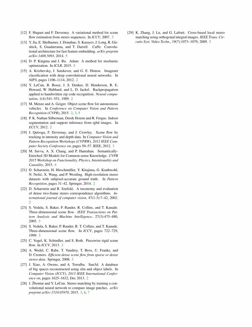
[29] K. Zhang, J. Lu, and G. Lafruit. Cross-based local stereomatching using orthogonal integral images. IEEE Trans. Cir-cuits Syst. Video Techn., 19(7):1073–1079, 2009. 3

A Large Dataset to Train Convolutional Networks for Disparity, Optical Flow,and Scene Flow Estimation: Supplementary Material

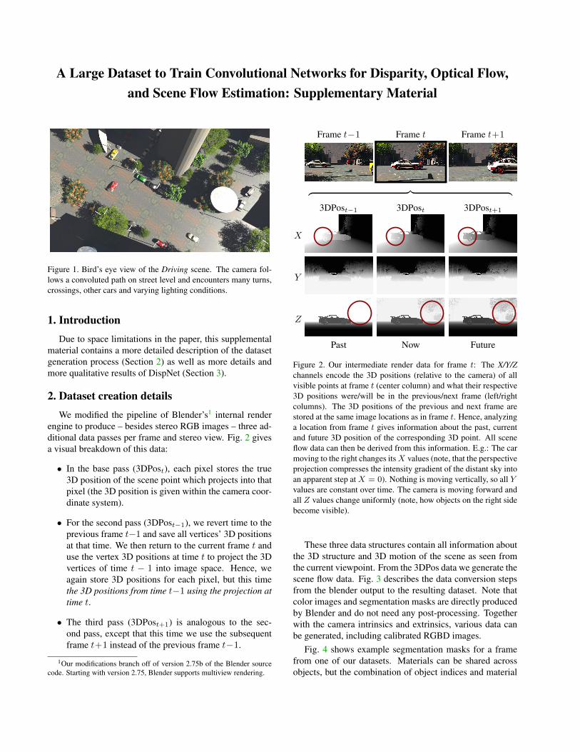
Figure 1. Bird’s eye view of the Driving scene. The camera fol-lows a convoluted path on street level and encounters many turns,crossings, other cars and varying lighting conditions.

1. IntroductionDue to space limitations in the paper, this supplemental

material contains a more detailed description of the datasetgeneration process (Section 2) as well as more details andmore qualitative results of DispNet (Section 3).

2. Dataset creation detailsWe modified the pipeline of Blender’s1 internal render

engine to produce – besides stereo RGB images – three ad-ditional data passes per frame and stereo view. Fig. 2 givesa visual breakdown of this data:

• In the base pass (3DPost), each pixel stores the true3D position of the scene point which projects into thatpixel (the 3D position is given within the camera coor-dinate system).

• For the second pass (3DPost−1), we revert time to theprevious frame t−1 and save all vertices’ 3D positionsat that time. We then return to the current frame t anduse the vertex 3D positions at time t to project the 3Dvertices of time t − 1 into image space. Hence, weagain store 3D positions for each pixel, but this timethe 3D positions from time t−1 using the projection attime t.

• The third pass (3DPost+1) is analogous to the sec-ond pass, except that this time we use the subsequentframe t+1 instead of the previous frame t−1.

1Our modifications branch off of version 2.75b of the Blender sourcecode. Starting with version 2.75, Blender supports multiview rendering.

Frame t−1 Frame t Frame t+1

︷ ︸︸ ︷3DPost−1 3DPost 3DPost+1

X

Y

Z

Past Now Future

Figure 2. Our intermediate render data for frame t: The X/Y/Zchannels encode the 3D positions (relative to the camera) of allvisible points at frame t (center column) and what their respective3D positions were/will be in the previous/next frame (left/rightcolumns). The 3D positions of the previous and next frame arestored at the same image locations as in frame t. Hence, analyzinga location from frame t gives information about the past, currentand future 3D position of the corresponding 3D point. All sceneflow data can then be derived from this information. E.g.: The carmoving to the right changes its X values (note, that the perspectiveprojection compresses the intensity gradient of the distant sky intoan apparent step at X = 0). Nothing is moving vertically, so all Yvalues are constant over time. The camera is moving forward andall Z values change uniformly (note, how objects on the right sidebecome visible).

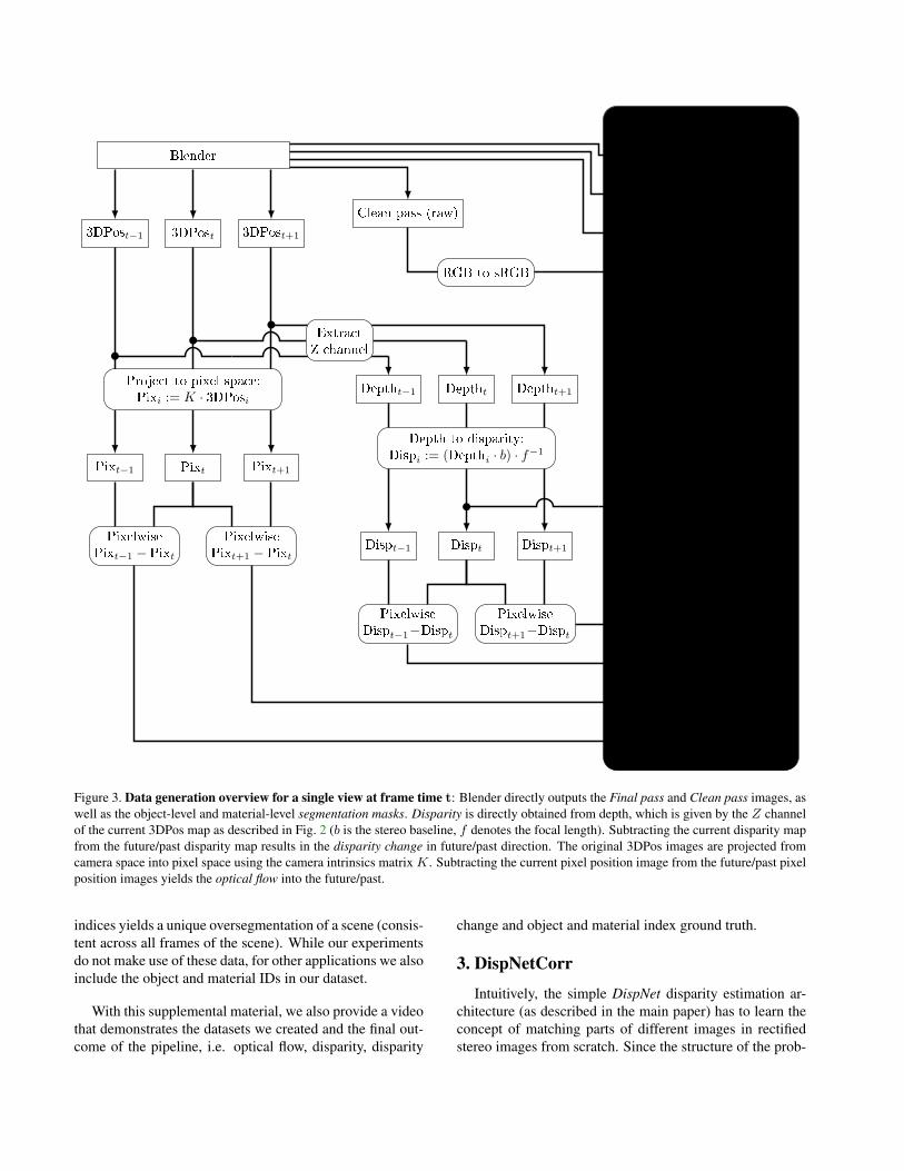
These three data structures contain all information aboutthe 3D structure and 3D motion of the scene as seen fromthe current viewpoint. From the 3DPos data we generate thescene flow data. Fig. 3 describes the data conversion stepsfrom the blender output to the resulting dataset. Note thatcolor images and segmentation masks are directly producedby Blender and do not need any post-processing. Togetherwith the camera intrinsics and extrinsics, various data canbe generated, including calibrated RGBD images.

Fig. 4 shows example segmentation masks for a framefrom one of our datasets. Materials can be shared acrossobjects, but the combination of object indices and material

Blender Final pass

Object segmentation

Material segmentation

Clean pass (raw)

Clean passRGB to sRGB

3DPost−1 3DPost 3DPost+1

Pixt−1 Pixt Pixt+1

Project to pixel space:Pixi := K · 3DPosi

PixelwisePixt−1 − Pixt

PixelwisePixt+1 − Pixt

Optical �ow into future

Optical �ow into past

Deptht−1 Deptht Deptht+1

ExtractZ channel

Dispt−1 Dispt Dispt+1

Depth to disparity:Dispi := (Depthi · b) · f−1

Disparity

PixelwiseDispt−1−Dispt

PixelwiseDispt+1−Dispt

Disp. change into future

Disp. change into past

OUTPUTS

Figure 3. Data generation overview for a single view at frame time t: Blender directly outputs the Final pass and Clean pass images, aswell as the object-level and material-level segmentation masks. Disparity is directly obtained from depth, which is given by the Z channelof the current 3DPos map as described in Fig. 2 (b is the stereo baseline, f denotes the focal length). Subtracting the current disparity mapfrom the future/past disparity map results in the disparity change in future/past direction. The original 3DPos images are projected fromcamera space into pixel space using the camera intrinsics matrix K. Subtracting the current pixel position image from the future/past pixelposition images yields the optical flow into the future/past.

indices yields a unique oversegmentation of a scene (consis-tent across all frames of the scene). While our experimentsdo not make use of these data, for other applications we alsoinclude the object and material IDs in our dataset.

With this supplemental material, we also provide a videothat demonstrates the datasets we created and the final out-come of the pipeline, i.e. optical flow, disparity, disparity

change and object and material index ground truth.

3. DispNetCorr

Intuitively, the simple DispNet disparity estimation ar-chitecture (as described in the main paper) has to learn theconcept of matching parts of different images in rectifiedstereo images from scratch. Since the structure of the prob-

Color image Object indices Material indices

Figure 4. Segmentation data: object indices are unique per scene.Material indices can be shared across objects, but can be combinedwith the object indices to yield an oversegmentation into parts.

lem is well known (correspondences can only be found inaccordance with the epipolar geometry [9]), we introducedan alternative architecture – the DispNetCorr – in which weexplicitly correlate features along horizontal scanlines.

While the DispNet uses two stacked RGB images as asingle input (i.e. one six-channel input blob), the Disp-NetCorr architecture first processes the input images sepa-rately, then correlates features between the two images andfurther processes the result. This behavior is similar to thecorrelation architecture used in [4] where Dosovitskiy et al.constructed a 2D correlation layer with limited neighbor-hood size and different striding in each of the images. Fordisparity estimation, we can use a simpler approach with-out striding and with larger neighborhood size, because thecorrelation along one dimension is computationally less de-manding. One can additionally reduce the amount of com-parisons by limiting the search to only one direction. Forexample, if we are given a left camera image and look forcorrespondences within the right camera image, then all dis-parity displacements are to the left.

Given two feature blobs a and b with multiple channelsand identical sizes, we compute a correlation map of thesame width and height, but with D channels, where D isthe number of possible disparity values. For one pixel atlocation (x, y) in the first feature blob a, the resulting cor-relation entry at channel d∈ [0, D − 1] is the scalar productof the two feature vectors a(x,y) and b(x−d,y).

4. Qualitative ExamplesWe show a qualitative evaluation of our networks for dis-

parity estimation and compare them to other approaches inFigures 5 to 10.

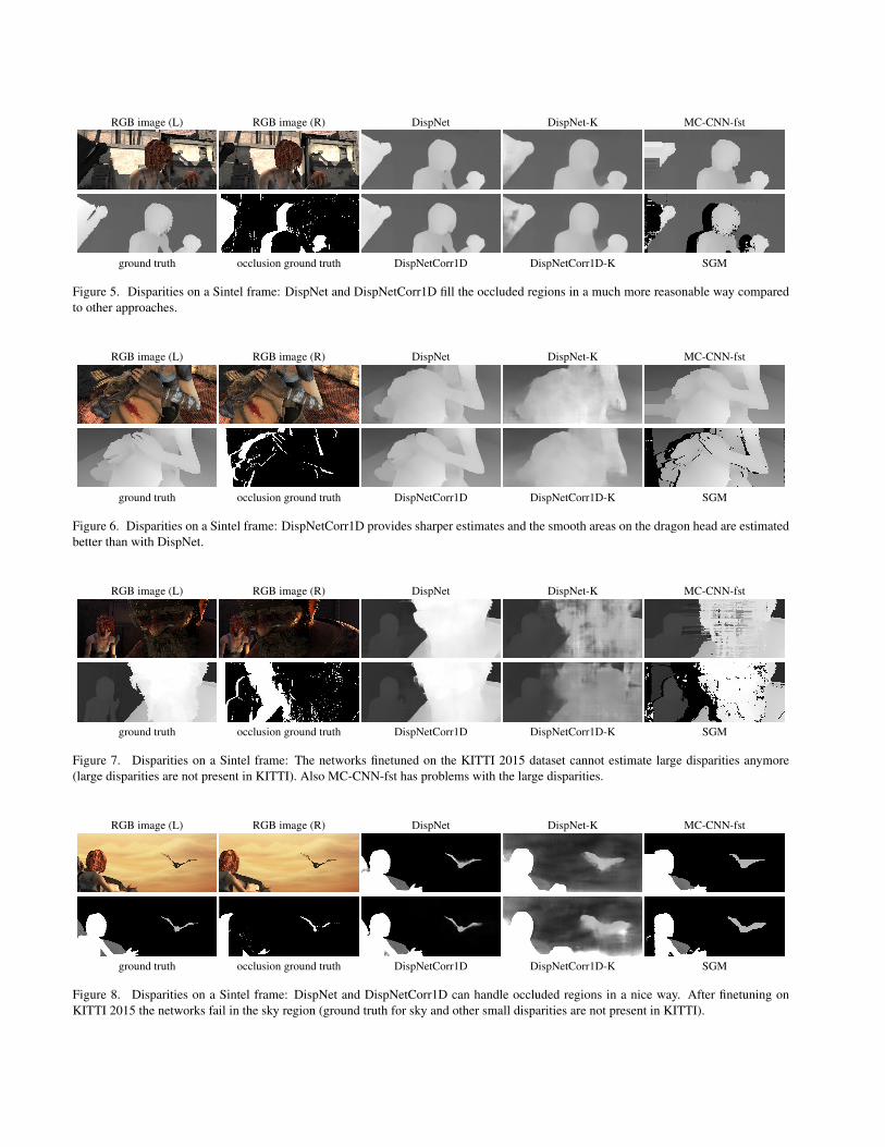
RGB image (L) RGB image (R) DispNet DispNet-K MC-CNN-fst

ground truth occlusion ground truth DispNetCorr1D DispNetCorr1D-K SGM

Figure 5. Disparities on a Sintel frame: DispNet and DispNetCorr1D fill the occluded regions in a much more reasonable way comparedto other approaches.

RGB image (L) RGB image (R) DispNet DispNet-K MC-CNN-fst

ground truth occlusion ground truth DispNetCorr1D DispNetCorr1D-K SGM

Figure 6. Disparities on a Sintel frame: DispNetCorr1D provides sharper estimates and the smooth areas on the dragon head are estimatedbetter than with DispNet.

RGB image (L) RGB image (R) DispNet DispNet-K MC-CNN-fst

ground truth occlusion ground truth DispNetCorr1D DispNetCorr1D-K SGM

Figure 7. Disparities on a Sintel frame: The networks finetuned on the KITTI 2015 dataset cannot estimate large disparities anymore(large disparities are not present in KITTI). Also MC-CNN-fst has problems with the large disparities.

RGB image (L) RGB image (R) DispNet DispNet-K MC-CNN-fst

ground truth occlusion ground truth DispNetCorr1D DispNetCorr1D-K SGM

Figure 8. Disparities on a Sintel frame: DispNet and DispNetCorr1D can handle occluded regions in a nice way. After finetuning onKITTI 2015 the networks fail in the sky region (ground truth for sky and other small disparities are not present in KITTI).

RGB image (L) DispNet DispNetCorr1D

RGB image (R) DispNet-K DispNetCorr1D-K

ground truth MC-CNN-fst SGM

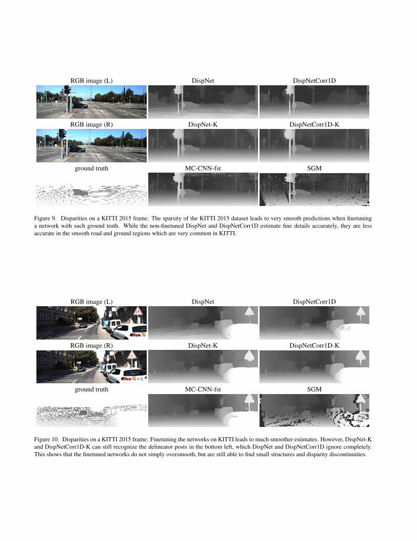
Figure 9. Disparities on a KITTI 2015 frame: The sparsity of the KITTI 2015 dataset leads to very smooth predictions when finetuninga network with such ground truth. While the non-finetuned DispNet and DispNetCorr1D estimate fine details accurately, they are lessaccurate in the smooth road and ground regions which are very common in KITTI.

RGB image (L) DispNet DispNetCorr1D

RGB image (R) DispNet-K DispNetCorr1D-K

ground truth MC-CNN-fst SGM

Figure 10. Disparities on a KITTI 2015 frame: Finetuning the networks on KITTI leads to much smoother estimates. However, DispNet-Kand DispNetCorr1D-K can still recognize the delineator posts in the bottom left, which DispNet and DispNetCorr1D ignore completely.This shows that the finetuned networks do not simply oversmooth, but are still able to find small structures and disparity discontinuities.