a knowledge-based method for temporal abstraction of clinical data
328
A KNOWLEDGE-BASED METHOD FOR TEMPORAL ABSTRACTION OF CLINICAL DATA A DISSERTATION SUBMITTED TO THE PROGRAM IN MEDICAL INFORMATION SCIENCES AND THE COMMITTEE ON GRADUATE STUDIES OF STANFORD UNIVERSITY IN PARTIAL FULFILLMENT OF THE REQUIREMENTS FOR THE DEGREE OF DOCTOR OF PHILOSOPHY By Yuval Shahar October 1994
Transcript of a knowledge-based method for temporal abstraction of clinical data

A KNOWLEDGE-BASED METHOD FOR TEMPORAL ABSTRACTION OF
CLINICAL DATA
A DISSERTATION
SUBMITTED TO THE PROGRAM IN MEDICAL INFORMATION SCIENCES
AND THE COMMITTEE ON GRADUATE STUDIES
OF STANFORD UNIVERSITY
IN PARTIAL FULFILLMENT OF THE REQUIREMENTS
FOR THE DEGREE OF
DOCTOR OF PHILOSOPHY
By
Yuval Shahar
October 1994

ii
© Copyright by Yuval Shahar 1994
All Rights Reserved

iii
I certify that I have read this dissertation and that in my opinion it is fullyadequate, in scope and quality, as a dissertation for the degree of Doctor ofPhilosophy.
___________________________________Mark A. Musen (Principal Adviser)(Departments of Medicine and Computer Science)
I certify that I have read this dissertation and that in my opinion it is fullyadequate, in scope and quality, as a dissertation for the degree of Doctor ofPhilosophy.
___________________________________Richard E. Fikes(Department of Computer Science)
I certify that I have read this dissertation and that in my opinion it is fullyadequate, in scope and quality, as a dissertation for the degree of Doctor ofPhilosophy.
___________________________________Barbara Hayes-Roth(Department of Computer Science)
Approved for the University Committee on Graduate Studies:
___________________________________

iv
Abstract
This dissertation describes a reasoning framework for knowledge-based systems,
that is specific to the task of abstracting higher-level concepts from time-stamped
data, but that is independent of any particular domain. I specify the theory
underlying the framework by a logical model of time, parameters, events, and
contexts: a knowledge-based temporal-abstraction theory. The domain-specific
knowledge requirements and the semantics of the inference structure that I
propose are well defined and can be instantiated for particular domains. I have
applied my framework to the domain of clinical medicine.
My goal is to create, from primary time-stamped patient data, interval-based
temporal abstractions, such as "severe anemia for 3 weeks in the context of
administering the drug AZT," and more complex patterns, involving several such
intervals. These intervals can be used for planning interventions for diagnostic
or therapeutic reasons, for monitoring plans during execution, and for creating
high-level summaries of electronic medical records. Temporal abstractions are
also helpful for explanation purposes. Finally, temporal abstractions can be a
useful representation for comparing a therapy planner’s recommendation with
that of the human user, when the goals in both plans can be described in terms of
creation, maintenance, or avoidance of certain temporal patterns.
I define a knowledge-based temporal-abstraction method that decomposes the
task of abstracting higher-level, interval-based abstractions from input data into
five subtasks . These subtasks are then solved by five separate, domain-
independent, temporal-abstraction mechanisms. The temporal-abstraction
mechanisms depend on four domain-specific knowledge types . The semantics
of the four knowledge types and the role they play in each mechanism are
defined formally. The knowledge needed to instantiate the temporal-abstraction
mechanisms in any particular domain can be parameterized and can be acquired
from domain experts manually or with automated tools.

v
I present a computer program implementing the knowledge-based temporal-
abstraction method: RÉSUMÉ . The architecture of the RÉSUMÉ system
demonstrates several computational and organizational claims with respect to
the desired use and representation of temporal-reasoning knowledge. The
RÉSUMÉ system accepts input and returns output at all levels of abstraction;
generates context-sensitive and controlled output; accepts and uses data out of
temporal order, modifying a view of the past or of the present, as necessary;
maintains several possible concurrent interpretations of the data; represents
uncertainty in time and value; and facilitates its application to additional
domains by editing only the domain-specific temporal-abstraction knowledge.
The temporal-abstraction knowledge is organized in the RÉSUMÉ system as
three ontologies (domain-specific theories of relations and properties) of
parameters, events, and interpretation contexts, respectively, in each domain.
I have evaluated the RÉSUMÉ system in the domains of protocol-based care,
monitoring of children’s growth, and therapy of insulin-dependent diabetic
patients. I have demonstrated that the knowledge required for instantiating the
temporal-abstraction mechanisms can be acquired in a reasonable amount of
time from domain experts, can be easily maintained, and can be used for creating
application systems that solve the temporal-abstraction task in these domains.
Understanding the knowledge required for abstracting clinical data over time is a
useful undertaking. A clear specification of that knowledge, and its
representation in an ontology specific to the task of abstracting concepts over
time, as was done in the architecture of the RÉSUMÉ system, supports designing
new medical and other knowledge-based systems that perform temporal-
reasoning tasks. The formal specification of the temporal-abstraction knowledge
also supports acquisition of that knowledge from domain experts, maintenance
of that knowledge once acquired, reusing the problem-solving knowledge for
temporal abstraction in other domains, and sharing the domain-specific
knowledge with other problem solvers that might need access to the domain’s
temporal-reasoning knowledge.

vi
Acknowledgments
My wife, Smadar, has been with me during the last three of my four graduate
degrees, over two continents and three academic centers. That alone would be
beyond most peoples’ endurance; yet, Smadar has always supported me in my
quest for combining the disciplines of computer science and medicine, was
amazingly patient, and has been a constant source of calmness. Our daughter,
Lilach proved to be equally patient, and even our son, Tomer, who has joined our
family only recently, has never been known to file a formal complaint.
No acknowledgments would be complete without mentioning the help in
continuing my graduate studies that I got, and the foundations in AI and general
mathematics and computer science that I learned, from my former mentors:
Larry Manevitz, Martin Golumbic, Larry Birnbaum and, especially, Jonathan
Stavi.
My main advisor, Mark Musen, has been supporting my ideas from the
beginning. Mark helped me find my way around the rather new academic
discipline of medical informatics, which turned out to be neither a subset of
medicine nor an extension of computer science, two areas I was familiar with.
Mark also was often my scientific editor, not an easy task. Barbara Hayes-Roth
was highly encouraging from the beginning of this work, was always an
excellent sounding board, and provided short but penetrating comments that
influenced greatly the organization of my work. Richard Fikes’ meticulous
examination of the details of my logical framework was immensely useful; it
forced me to clarify my ideas so that the casual, though technical, reader can
understand them unambiguously. Finally, a fourth, though unofficial, important
reader and advisor of this thesis was Michael Kahn. Michael encouraged my
interest in temporal reasoning in medicine, an area to which he himself
contributed greatly, and agreed from the beginning of this research to support it
with his advice; his comments were always sound and practical. I have also

vii
found in Michael’s Ph.D. thesis a model of clarity in writing and organization
that I have tried, at least, to emulate.
I have enjoyed greatly my stay at Stanford and its great environment—both its
weather and its people. I feel indebted to Ted Shortliffe for arriving at that
environment. I have been corresponding with Ted several years before I had
arrived at Stanford, and it was due to his vision in creating the program in
medical informatics and being the driving force behind it that I realized that my
interests lay in this new interdisciplinary area. Ted also facilitated greatly my
arrival at Stanford. Finally, when I was forming my thesis proposal, I found my
discussions with Ted about his concepts as to how a proposal should look and
the way it should be developed into a thesis as highly practical and useful.
Working with everybody in the PROTÉGÉ-II/T-Helper gang was (and still is) a
great experience. In particular, I would like to thank Samson Tu for all the
detailed conversations we had on planning and temporal reasoning in medicine,
which helped me greatly in focusing and implementing my ideas. Henrik
(“super hacker”) Eriksson was always a great help too. I had also spent many
pleasant hours discussing decision-analysis and other issues with John Egar.
Finally, I had many highly relevant technical discussions with Amar Das, who is
another brotherly spirit in the area of temporal reasoning in medicine, and who
helped me find many of the reference sources.
My written work would surely be unreadable if not for Lyn Dupré’s industrious
editing of my papers over the years and of my drafts of this thesis. My friend
Lynne Hollander often helped in this task, and supplied general encouragement
and many interesting discussions. With respect to support and encouragement, I
feel indebted also to Betty Riccio, Darlene Vian, Pat Swift and the excellent
technical support of the SSRG group.
Most of my work had been supported by the T-Helper project, funded under
Grant No. HS06330 from the Agency for Health Care Policy and Research. The
computing resources were provided by the Stanford CAMIS project, funded
under Grant No. LM05305 from the National Library of Medicine.

viii
Contents
Abstract.......................................................................................................................... iv
Acknowledgments........................................................................................................ vi
Contents......................................................................................................................... viii
List of Tables................................................................................................................. xii
List of Figures............................................................................................................... xiii
List of Symbols............................................................................................................. xv
1 Introduction: The Temporal-Abstraction Task.................................................. 1
1.1 The Temporal Abstraction Task in Clinical Domains............................... 5
1.2 The Temporal-Abstraction Method and Its Mechanisms......................... 9
1.2.1 Temporal Reasoning in Philosophy and Computer Science........... 10
1.2.2 The Knowledge-Based Temporal-Abstraction Method................... 12
1.2.2.1 The Context-Forming Mechanism.............................................. 16
1.2.2.2 The Contemporaneous-Abstraction Mechanism...................... 17
1.2.2.3 The Temporal-inference Mechanism......................................... 18
1.2.2.4 The Temporal-Interpolation Mechanism................................... 19
1.2.2.5 The Temporal-Pattern—Matching Mechanism....................... 20
1.3 The RÉSUMÉ System...................................................................................... 21
1.4 Problem-Solving Methods and Knowledge Acquisition........................... 24
1.5 Summary........................................................................................................... 26
1.6 A Map of the Dissertation............................................................................... 27
2 Problem-Solving Methods and Knowledge Acquisition in ClinicalDecision-Support Systems.............................................................................. ....... 30
2.1 The Knowledge Level and Problem-Solving Methods.............................. 32
2.2 Automated Knowledge-Acquisition Tools and the PROTÉGÉ-II Project 37
2.3 Discussion and Summary............................................................................... 43
3 Temporal Reasoning in Clinical Domains............................................................. 45
3.1 Temporal Ontologies and Temporal Models............................................... 47
3.1.1 Tense Logics............................................................................................. 47
3.1.2 Kahn and Gorry’s Time Specialist........................................................ 51
3.1.3 Approaches Based on States, Events, or Changes.............................. 52
3.1.3.1 The Situation Calculus and Hayes’ Histories............................. 52

ix
3.1.3.2 Dynamic Logic................................................................................ 53
3.1.3.3 Qualitative Physics......................................................................... 54
3.1.3.4 Kowalski and Sergot’s Event Calculus....................................... 54
3.1.4 Allen’s Interval-based Temporal Logic and Related Extensions..... 55
3.1.5 McDermott’s Point-Based Temporal Logic......................................... 59
3.1.6 Shoham’s Temporal Logic..................................................................... 60
3.1.7 The Perspective of the Database Community.................................... 62
3.1.8 Representing Uncertainty in Time and Value.................................... 65
3.1.8.1 Modeling of Temporal Uncertainty............................................ 66
3.1.8.2 Projection, Forecasting, and Modeling the PersistenceUncertainty................................................................................... 69
3.2 Temporal Reasoning Approaches in Clinical Domains............................. 72
3.2.1 Encapsulation of Temporal Patterns as Tokens................................. 73
3.2.1.1 Encapsulation of Time as Syntactic Constructs........................ 74
3.2.2 Encapsulation of Time as Causal Links.............................................. 74
3.2.3 Fagan’s VM Program: A State-Transition Temporal-Interpretation System.......................................................................... 75
3.2.4 Temporal Bookkeeping: Russ’s Temporal Control Structure.......... 78
3.2.5 Discovery in Time-Oriented Clinical Databases: Blum’s Rx Project 83
3.2.6 Down’s Program for Summarization of On-Line Medical Records 86
3.2.7 De Zegher-Geets’ IDEFIX Program for Medical-RecordSummarization............................................................................... ....... 88
3.2.8 Rucker’s HyperLipid System............................................................... 93
3.2.9 Qualitative and Quantitative Simulation........................................... 94
3.2.9.1 The Digitalis-Therapy Advisor................................................... 94
3.2.9.2 The Heart-Failure Program.......................................................... 94
3.2.10 Kahn’s TOPAZ System: An Integrated Interpretation Model....... 96
3.2.11 Kohane’s Temporal-Utilities Package (TUP)................................... 102
3.2.12 Haimovitz’s and Kohane’s TrenDx System..................................... 105
3.2.13 Larizza’s Temporal-Abstraction Module in the M-HTPSystem.............................................................................................. ..... 109
3.3 Discussion........................................................................................................ 113
4 Knowledge-based Temporal Abstraction............................................................ 117
4.1 The Temporal-Abstraction Ontology.......................................................... 118
4.2 The Temporal-Abstraction Mechanisms..................................................... 133

x
4.2.1 The Context-Forming Mechanism...................................................... 137
4.2.2 Contemporaneous Abstraction........................................................... 146
4.2.3 Temporal Inference............................................................................... 148
4.2.4 Temporal Interpolation......................................................................... 156
4.2.4.1 Local and Global Persistence Functions and Their Meaning. 166
4.2.4.1.1 Local Persistence Functions............................................... 167
4.2.4.1.2 Global Persistence Functions.............................................. 169
4.2.4.1.3 A Typology of ∆ Functions................................................. 172
4.2.5 Temporal-Pattern Matching................................................................. 176
4.2.6 The Nonmonotonicity of Temporal Abstractions............................. 179
4.3 Discussion and Summary.............................................................................. 182
5. The RÉSUMÉ System............................................................................................. 187
5.1 The Parameter-Properties Ontology........................................................... 188
5.1.1 Dimensions of Classification Tables................................................... 195
5.1.1.1 Table Axes..................................................................................... 198
5.1.2 Sharing of Parameter Propositions Among Different Contexts.... 201
5.2 The Context-Forming Mechanism and the Event and ContextOntologies....................................................................................... ..... 203
5.3 The Temporal-Abstraction mechanisms in the RÉSUMÉ System.......... 211
5.3.1 Control and Computational Complexity of the RÉSUMÉ System 211
5.4 The Temporal Fact Base and Temporal-Pattern Matching....................... 214
5.5 The Truth-Maintenance System.................................................................. 218
5.6 Discussion and Summary............................................................................ 220
6. Application of Knowledge-Based Temporal Abstraction.............................. 222
6.1 Protocol-Based Care...................................................................................... 224
6.2 Monitoring of Children’s Growth............................................................... 227
6.3 The Diabetes-Monitoring Domain.............................................................. 235
6.4 Discussion and Summary............................................................................ 249
7. Acquisition of Temporal-Abstraction Knowledge........................................... 257
7.1 Manual Acquisition of Temporal-Abstraction Knowledge.................... 258
7.2 Automated Acquisition of Temporal-Abstraction Knowledge.............. 261
7.3 Knowledge Acquisition Using Machine Learning................................... 266
7.4 Discussion and Summary............................................................................. 268
8. Summary and Discussion.................................................................................... 270

xi
8.1 Summary of This Dissertation.................................................................... 271
8.2 The RÉSUMÉ System and the Temporal-Abstraction Desiderata......... 275
8.2.1 Accepting as Input Data of Multiple Types and AbstractionLevels.................................................................................................... 275
8.2.2 Availability of Output Abstractions at All Levels of Abstraction. 276
8.2.3 Context-Sensitive Interpretation........................................................ 277
8.2.4 Acceptance of Data Out of Temporal Order..................................... 278
8.2.5 Maintenance of Several Concurrent Interpretations....................... 278
8.2.6 Enablement of Temporal and Value Uncertainty............................ 279
8.2.7 Facilitation of Development, Acquisition, Maintenance,Sharing and Reuse of the Knowledge Base................................ ..... 279
8.2.8 Separation of Interpretation from Planning..................................... 280
8.2.9 Summarization of Medical Records................................................... 280
8.2.10 Provision of Explanations................................................................. 281
8.2.11 Support of Plan Recognition and Human-ComputerCollaboration.................................................................................. ..... 281
8.3 RÉSUMÉ and Other Clinical Temporal-Reasoning Systems.................. 282
8.3.1 Conclusions from Comparison to Other Approaches.................... 286
8.4 Implications and Extensions of the Work................................................. 288
8.4.1 Implications for Knowledge Acquisition......................................... 288
8.4.2 Implications for a Broader Temporal-Reasoning Architecture.... 289
8.4.3 Implications of the Nonmonotonicity of Temporal Abstractions. 290
8.4.4 The Threshold Problem....................................................................... 292
8.4.5 Implications for Semantics of Temporal Databases........................ 293
8.4.6 Relationship to Other Knowledge-Based Problem-SolvingFrameworks.................................................................................... ..... 294
8.4.7 Implications for Plan Recognition and Critiquing........................... 296
8.5 Summary......................................................................................................... 296
Bibliography................................................................................................................ 299

xii
List of Tables
4.1 The default horizontal-inference join (⊕ ) operation for the gradientabstraction type.................................................................................................... 155
4.2 An interpolation-inference table representing the secondary temporal-interpolation operation for extending a DECREASING value of thegradient abstraction............................................................................................. 161
5.1 Some of the slots in the frame of the Hb_Gradient_CCTG parameter........ 194
5.2 A 4:1 (numeric and symbolic to symbolic) maximal-OR range table forthe SYSTEMIC TOXICITY parameter in the context of the CCTG-522experimental AIDS-treatment protocol....................................................... ..... 200
6.1 Abstractions formed by the pediatric endocrinologist and by theRÉSUMÉ system in the domain of monitoring children’s growth.......... ..... 234
6.2 Abstractions formed by the two experts in the diabetes domain.................. 245
6.3 Therapy recommendations made by the diabetes experts............................. 248

xiii
List of Figures
1.1 Inputs to and outputs of the temporal-abstraction task................................ 6
1.2 The knowledge-based temporal-abstraction method.................................... 14
1.3 Inducing an interpretation context by an event............................................. 16
1.4 Contemporaneous abstraction.......................................................................... 17
1.5 The temporal-inference mechanism................................................................. 18
1.6 The temporal-interpolation mechanism.......................................................... 19
1.7 A temporal-pattern parameter.......................................................................... 20
1.8 A schematic view of the RÉSUMÉ system architecture................................ 22
2.1 The heuristic-classification inference structure.............................................. 35
2.2 Decomposition of the task of managing patients on clinical protocolsby the ESPR method....................................................................................... .... 39
3.1 The 13 possible relations defined by Allen between temporal intervals... 56
3.2 A nonconvex interval........................................................................................ 58
3.3 A variable interval............................................................................................. 67
3.4 The TCS system’s rule environment............................................................... 79
3.5 Partitioning the database by creation of stable intervals in the TCS system 80
3.6 A chain of processes in the TCS system......................................................... 81
3.7 The knowledge base of Downs’ summarization program.......................... 87
3.8 A time-oriented probabilistic function (TOPF)............................................. 90
3.9 Summarization of time-ordered data in the TOPAZ system...................... 97
3.10 A range relation (RREL)................................................................................. 103
3.11 A portion of a trend template (TT) in TrenDx............................................. 106
3.12 A portion of the M-HTP visits taxonomy..................................................... 110
3.13 A portion of the M-HTP significant-episodes taxonomy.............................. 111
4.1 Processing of parameter points and intervals by the temporal-abstraction mechanisms................................................................................. ... 136
4.2 Dynamic induction relations of context intervals (DIRCs).......................... 140
4.3 Local and global persistence functions........................................................... 168
5.1 The RÉSUMÉ system’s general architecture.................................................. 189
5.2 A portion of the RÉSUMÉ parameter-properties ontology for thedomain of protocol-based care......................................................................... 191

xiv
5.3 A portion of the event ontology in the protocol-management domain..... 207
5.4 A portion of the context ontology in the protocol-management domain.. 209
6.1 Abstraction of platelet and granulocyte counts during administrationof a prednisone/azathioprine (PAZ) protocol........................................... ..... 226
6.2 Part of the parameter-properties ontology for the domain ofmonitoring children’s growth........................................................................... 229
6.3 Part of the result of running RÉSUMÉ in the domain of monitoringchildren’s growth, using the acquired parameter-properties ontology,on case 1........................................................................................................... .... 232
6.4 Part of the diabetes parameter-properties ontology...................................... 236
6.5 Part of the diabetes event ontology.................................................................. 237
6.6 Part of the diabetes context ontology............................................................... 238
6.7 Formation of contexts in the diabetes-treatment domain............................. 239
6.8 One of the charts representing data from Case 30.......................................... 241
6.9 A portion of a spreadsheet representing data from Case 30......................... 242
6.10 Abstraction of data by RÉSUMÉ in Case 3.................................................... 244

xv
List of Symbols
PART-OF (small caps) a relation name
∈ The ELEMENT-OF relation
≥ The GREATER-OR-EQUAL-TO relation
≤ The LESS-THEN-OR-EQUAL-TO relation
≡ Equivalence relation
∀ Universal quantifier (i.e., FOR ALL)
∃ Existential quantifier (i.e., THERE EXISTS)
∧ Logical conjunction (i.e., AND)
∨ Logical disjunction (i.e., OR)
¬ Logical-negation (i.e., NOT)
=> Logical-implication (i.e., IMPLIES)
<....> A structure
ƒ() A function
τ ∈ Τ A time stamp and its symbol set
-∞, +∞ The past and future time stamps
* The “wild-card” time stamp
Gi ∈ Γ A temporal-granularity unit and its symbol set
I A time interval
Ti A time point
π ∈Π A parameter and its symbol set
e ∈ Ε An event and its symbol set
ai An event argument
e The natural-logarithm base
ξ ∈ Ξ An interpretation context and its symbol set
ψ ∈ Ψ An abstraction-goal proposition and its symbol set
ϕ ∈ Ρ Any temporal-abstraction proposition and its symbol set
θ ∈ Θ An abstraction function and its symbol set
ν A (symbolic) parameter or event-argument value
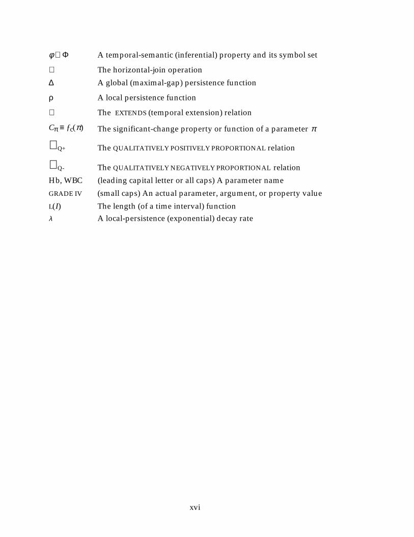
xvi
φ ∈ Φ A temporal-semantic (inferential) property and its symbol set
⊕ The horizontal-join operation
∆ A global (maximal-gap) persistence function
ρ A local persistence function
⇔ The EXTENDS (temporal extension) relation
Cπ ≡ ƒc(π) The significant-change property or function of a parameter π
∝ Q+ The QUALITATIVELY POSITIVELY PROPORTIONAL relation
∝ Q- The QUALITATIVELY NEGATIVELY PROPORTIONAL relation
Hb, WBC (leading capital letter or all caps) A parameter name
GRADE IV (small caps) An actual parameter, argument, or property value
L(I) The length (of a time interval) functionλ A local-persistence (exponential) decay rate

Chapter 1: The Temporal Abstraction Task
1
1 Introduction:
The Temporal-Abstraction Task
There are many domains of human endeavor that require the collection of
substantial amounts of data over time and the abstraction of those data into
higher-level concepts, meaningful in that domain. In my dissertation, I have
investigated the nature of this task, the type of knowledge required for solving it
in uniform fashion in different domains, and how that knowledge should be
represented and used. I have focused in my examples on several subdomains of
clinical medicine, in which the task of abstraction of data over time occurs
frequently. Most of the ideas I shall discuss, however, are quite general, and are
applicable to other domains in which data need to be interpreted over time.
Most clinical tasks require measurement and capture of numerous patient data.
Methods for storing these data in specialized medical-record databases are
evolving. However, physicians who have to make diagnostic or therapeutic
decisions based on these data may be overwhelmed by the number of data if the
physicians’ ability to reason with the data does not scale up to the data-storage
capabilities. Furthermore, most of these data include a time stamp in which the
particular datum was valid; and an emerging pattern over a stretch of time has
much more significance than an isolated finding or even a set of findings. The
ability to combine several significant contemporaneous findings and to abstract
them into clinically meaningful higher-level concepts in a context-sensitive
manner, ignoring less significant data, and the ability to detect significant trends
in both low-level data and abstract concepts, are hallmarks of the experienced
physician.
Thus, it is highly desirable for an automated, knowledge-based medical decision-
support tool that assists physicians who monitor patients over significant
periods, to provide short, informative summaries of clinical data stored on

Chapter 1: The Temporal Abstraction Task
2
electronic media, and to be able to answer queries about abstract concepts that
summarize the data. Providing these abilities would benefit both a human
physician and an automated decision-support tool that recommends therapeutic
and diagnostic measures based on the patient's clinical history up to the present.
Such concise, meaningful summaries, apart from their immediate intrinsic value,
support the automated system’s further recommendations for diagnostic or
therapeutic interventions, provide a justification for the system’s or for the
human user’s actions, and monitor plans suggested by the physician or by the
decision-support system. Such a meaningful summary cannot use only time
points, such as dates when data were collected; it must be able to characterize
significant features over periods of time, such as "5 months of decreasing liver
enzyme levels in the context of recovering from hepatitis." I refer to such periods
as intervals of time, and to the high-level characterizations attached to these
intervals as abstractions .
However, most medical decision-support systems, including most knowledge-
based ones, either do not represent detailed temporal information about the data
at all, or do not have sufficient general temporal-reasoning knowledge to enable
reasoning about temporal relations explicitly. The few systems that include
temporal-reasoning capability encode both the general temporal-reasoning
knowledge and the temporal-reasoning knowledge specific to the particular
clinical domain in application-specific rules and functions using procedural
representations, such as arbitrary code. Other approaches in clinical information
systems supply a general procedural syntax for clinical algorithms, and even
provide data types for time points or intervals, but do not allow for any
predefined semantic aspects (e.g., the concept of a SIGNIFICANT CHANGE OVER
TIME) that are specific to the task of abstracting higher-level concepts from time-
stamped data, but that are independent of the particular application domain.
Such representations often rely on the particular terms of the domain they
represent, as well as on the particular terms of the task in which they are being
used; sometimes, they even rely on the particular institution at which they are
used (e.g., the clinical parameter SERUM POTASSIUM might have a different label
in different hospitals).

Chapter 1: The Temporal Abstraction Task
3
The use of such domain-specific approaches enables little reuse of the underlying
domain-independent temporal-reasoning knowledge for other domains; neither
does it enable sharing the domain-specific temporal-reasoning knowledge
accumulated for the particular encoded task with other tasks and problem-
solving methods involving some kind of reasoning about time in the same
domain. For instance, it is correct to infer from two consecutive episodes of
fever, each lasting 1 week, that the patient had an episode of fever lasting 2
weeks. In addition, a conclusion of having a 3-week fever might be valid in
certain contexts when there was a nonmonitored gap of a week between the two
1-week fever episodes, but probably not if the gap was more than a month.
However, it is definitely not the case that two episodes of pregnancy, each lasting
9 months, can be abstracted into a longer pregnancy episode of 18 or more
months, even if the two episodes could happen consecutively. Such reasoning
uses knowledge about the temporal-semantic properties of the clinical parameters
involved, knowledge that is specific for a particular domain (e.g., a clinical area)
of application, and that is crucial for the domain-independent task of temporal
abstraction. Most knowledge-based systems do not represent this knowledge
explicitly, although it is used implicitly. In addition, due to the idiosyncratic
nature of the knowledge-representation scheme of temporally oriented
knowledge used in most systems, it is difficult to acquire the required knowledge
from expert physicians in a uniform, well-defined way, or to maintain that
knowledge, once acquired. Finally, if an explicit representation of that
knowledge is lacking, it is even more difficult to construct an automated
knowledge-acquisition tool that might be used directly by an expert physician to
build the required medical knowledge base. Constructing such tools, when
possible, has been shown to have major benefits, mainly in facilitating the
acquisition of knowledge without the intervention of a knowledge engineer.
This dissertation concerns a reasoning method and its required knowledge, that
are specific to the task of abstracting higher-level concepts from time-stamped
data in knowledge-based systems, but independent of any particular domain. I
specify the theory underlying the method in a general, domain-independent way
by a logical model of time, events (e.g., administration of a drug ) parameters

Chapter 1: The Temporal Abstraction Task
4
(e.g., platelet count), and the contexts these entities create for interpretation of
data (e.g., a period of chemotherapy effects): a knowledge-based temporal-
abstraction theory. Thus, the domain-specific requirements and semantics of the
method I propose are well defined and can be easily customized for particular
domains. My goal is to create, from input time-stamped data, interval-based
temporal abstractions, such as "severe anemia for 3 weeks in the context of
administering the drug AZT," as well as abstractions defined by more complex
patterns, involving several such intervals. These intervals can be used for
planning interventions for diagnostic or therapeutic reasons, for monitoring
therapy plans during execution, and for creating high-level summaries of
medical records that reside on a clinical database. Temporal abstractions are also
helpful for explanation purposes. Finally, temporal abstractions can be a useful
representation for comparing the system’s recommended plan with that of the
human user, when the overall and intermediate goals in both plans can be
described in terms of creating and maintaining certain temporal patterns.
My methodology involves defining a knowledge-based temporal-abstraction
method that decomposes the task of abstracting higher-level, interval-based
abstractions from input data into several subtasks . These subtasks are then
performed by several separate, domain-independent, temporal-abstraction
mechanisms . The temporal-abstraction mechanisms depend on four domain-
specific knowledge types. I define the independent mechanisms composing the
temporal-abstraction method in a formal, uniform, explicit way, such that the
knowledge needed to instantiate them in any particular domain and task can be
parameterized and acquired from domain experts manually, with automated
tools, or by other methods (e.g., machine learning). I organize the domain-
specific knowledge required for instantiating the temporal-abstraction
mechanisms as four separate types (or categories) to emphasize the nature of the
knowledge contained in each category and the role that knowledge plays in the
reasoning performed by each mechanism.
The temporal-abstraction mechanisms that I suggest can be packaged together
(as when used by the knowledge-based temporal-abstraction method) or used

Chapter 1: The Temporal Abstraction Task
5
separately; thus some, or all, of them can be configured within a more general
problem solver, such as a therapy planner. The domain-specific knowledge they
use has clear semantics and can be shared with other applications in the same
domain that require similar types of temporal reasoning.
1.1 The Temporal-Abstraction Task in Clinical Domains
Consider the following task: Given time-stamped patient data and several
clinical events (e.g., therapy administration), possibly accumulated over a long
time, produce an analysis of the data that interprets past and present states and
trends and that is relevant for clinical decision-making purposes in the given or
implied clinical contexts. The clinical decision-making purposes usually include
determining an intermediate-level, temporal-interval-based diagnosis (e.g., "a
period of 5 weeks of grade III toxicity of the bone marrow due to the effects of
the therapy," or "an abnormal growth pattern between the ages of 2 and 15 years,
compatible with a constitutional growth delay"). The overall diagnosis, such as
“AIDS” or “diabetes” is often part of the input, providing a context within which
meaningful abstractions are formed. Figure 1.1 shows an example of a possible
input for the temporal-abstraction task, and the resulting output, in the case of a
patient who is receiving a clinical regimen for treatment of chronic graft-versus-
host disease (GVHD), a complication of bone-marrow transplantation.
The goals of the temporal-abstraction task may be to evaluate and summarize the
state of the patient over a time interval (possibly, the full span of the patient’s
known record), to identify various possible problems, to assist in a revision of an
existing therapy plan, or to support a generation of a new plan. In addition,
generation of meaningful intervals supports the task of explaining the system’s
plans and actions to several different classes of users (e.g., a resident physician, a
nurse, an experienced clinical expert). Finally, representation of overall goals
(policies), as well as intermediate ones, as temporal patterns to be achieved or
avoided, enables comparison between the plans generated by a knowledge-based
system and plans suggested by a user, and supports monitoring the progress of
either type of plan. Many of these goals are typical to guideline-based therapy .

Chapter 1: The Temporal Abstraction Task
6
.
•
0 40020010050
•
∆∆
1000
2000
∆( )∆ ∆ ∆
100K
150K
( )
•••
• • • •∆∆∆•
••
∆∆∆∆∆∆•••
Granu-locytecounts
• • •∆ ∆∆ ∆
•
Time (days)
Plateletcounts
PAZ protocol|
BMT
(a)
•
0 40020010050
•
∆∆
1000
2000∆( )∆ ∆ ∆
100K
150K
( )
•••
• • • •∆∆∆•
• •
∆∆∆∆∆∆•••
Granu-locytecounts
• • •∆ ∆∆ ∆
•
Time (days)
Plateletcounts
PAZ protocol
ExpectedCGVHD
M[0] M[1] M[2] M[3] M[0] M[0]
(b)
Figure 1.1: Inputs to and outputs of the temporal-abstraction task.
(a) Platelet and granulocyte counts during administration of a prednisone/azathioprine (PAZ)
protocol for treating patients who have chronic graft-versus-host disease (CGVHD). =
event; • = platelet counts; ∆ = granulocyte counts. The time line starts with the bone-marrow
transplantation (BMT) event. This input is typical for temporal-abstraction tasks.
(b) Abstraction of the platelet and granulocyte counts shown in Figure 1.1a. = closed
context interval; = open context interval; = closed abstraction interval; M[n ] =
myelotoxicity grade n . Both types of intervals are typically part of the output of a method solving
the temporal-abstraction task.

Chapter 1: The Temporal Abstraction Task
7
There are several points to note with respect to the desired computational
behavior of a method that creates meaningful abstractions from time-stamped
data:
1. The method should be able to accept as input both numeric and qualitative data.
Some of these data might be at different levels of abstraction (i.e., we might be given
either raw data or higher-level concepts as primary input, perhaps abstracted by
the physician from the same or additional data). The data might also involve
different forms of temporal representation (e.g., time points or time intervals).
2. The output abstractions should also be available for query purposes at all levels
of abstraction, and should be created as time points or as time intervals, as
necessary, aggregating relevant conclusions together as much as possible (e.g.,
"extremely high blood pressures for the past 8 months in the context of treatment
of hypertension"). The outputs generated by the method should be controlled,
sensitive to the goals of the abstraction process for the task at hand (e.g., only
particular types of output might be required). The output abstractions should
also be sensitive to the context in which they were created.
3. Input data should be used and incorporated in the interpretation even if they
arrive out of temporal order (e.g., a laboratory result from last Tuesday arrives
today). Thus, the past can change our view of the present. I call this
phenomenon a view update. Furthermore, new data should enable us to reflect
on the past; thus, the present (or future) can change our interpretation of the past,
a property referred to as hindsight [Russ, 1989].
4. Several possible interpretations of the data might be reasonable, each
depending on additional factors that are perhaps unknown at the time (such as
whether the patient has AIDS); interpretation should be specific to the context in
which it is applied. All reasonable interpretations of the same data relevant to
the task at hand should be available automatically or upon query.

Chapter 1: The Temporal Abstraction Task
8
5. The method should leave room for some uncertainty in the input and the
expected data values, and some uncertainty in the time of the input or the
expected temporal pattern.
6. The method should be generalizable to other clinical domains and tasks. The
domain-specific assumptions underlying it should be explicit and as declarative
as possible (as opposed to procedural code), so as to enable reuse of the method
without rebuilding the system, acquisition of the necessary knowledge for
applying it to other domains, maintenance of that knowledge, and sharing that
knowledge with other applications in the same domain.
An example of a common clinical problem in which the temporal-abstraction task
plays a central role is the management of patients who are being treated
according to clinical protocols. Clinical protocols are therapy guidelines for
particular diseases and clinical conditions, that usually prescribe a detailed and
complex set of rules that the physician should follow. Apart from the benefit of
using expert knowledge accumulated over years, using such standard protocols
allows potential therapeutic regimens to be compared and evaluated. An
inherent requirement of protocol-based care is to accumulate and analyze large
amounts of patient data, sometimes including many dozens of clinical
parameters (laboratory test results, physical findings, assessments by physicians)
over time, in the context of one or more treatment protocols (see Figure 1.2). The
goal is to revise continuously an assessment of the patient’s condition by
abstracting higher-level features and states (e.g., a drug-toxicity state) from raw
numerical and qualitative data at various levels of abstraction (e.g., hemoglobin
[Hb] values). These higher-level features can be used in monitoring the effects of
the interventions indicated by the protocol, in recognizing problems, and in
suggesting possible modifications to the original treatment plan. Examples of
knowledge-based systems designed solely for the task of assisting physicians
treating patients by clinical protocols include ONCOCIN in the oncology domain
[Tu et al., 1989], and T-HELPER in the AIDS domain [Musen et al., 1992a].

Chapter 1: The Temporal Abstraction Task
9
Answering the typical protocol-related question “Did the patient have a period
of 3 or more weeks of bone-marrow toxicity, Grade II, within the past 6 months,
during the administration of the PAZ protocol?” requires the abilities (1) to
abstract levels of bone-marrow toxicity from several parameters and events; (2)
to bridge the temporal gaps among several data points and intervals, in order to
create longer meaningful intervals; and (3) to reason about relationships among
various temporal intervals, including physical events (e.g., drug administration)
as well as abstracted data (e.g., “moderate granulocyte toxicity”). Note that only
some of this knowledge is represented explicitly in any particular clinical
protocol. A major part of this knowledge is implicit in the underlying
assumptions of the protocol designer, including the protocol-interpreting
capabilities of the patient's own physician.
In Chapter 3, I discuss previous approaches to temporal reasoning in medicine in
general and to the temporal-abstraction task in particular. I point out features of
these approaches that allow comparison to my methodology. Further
comparisons with previous approaches are made in the context of discussions of
my work appearing at the end of Chapters 4 through 7. A summary of all
comparisons to other approaches appears in Section 8.3. Each of the previous
approaches has various advantages and disadvantages. None of them, however,
focuses on the knowledge-acquisition, knowledge-maintenance, knowledge-
reuse, or knowledge-sharing aspects of designing and building large knowledge-
based medical systems that are designed to deal with temporal aspects of clinical
data.
1.2 The Temporal-Abstraction Method and Its Mechanisms
Since a major emphasis of this work is reasoning about time, it is useful to
discuss briefly how time might be represented at all in computer applications,
and what are some of the difficulties inherent in temporal reasoning. In
Chapter 3, I delve more deeply into the details of various temporal-reasoning
approaches and computer systems in general, and of approaches applied to
clinical domains in particular. Here I present only a brief overview.

Chapter 1: The Temporal Abstraction Task
10
1.2.1 Temporal Reasoning in Philosophy and Computer Science
Philosophers, linguists, and logicians have been debating the best representation
of the concept of time, and the best means of reasoning about time, for at least
2500 years. For instance, Aristotle was occupied by the meaning of the truth
value of future propositions; the stoic logician Diodorus Cronus, following
Aristotle's methods, constructed the master argument that tried to conclude that
every possibility is realized in the past or the future [Rescher and Urquhart,
1971]. A landmark work by Prior [1955] attempted to reconstruct the Diodorian
master argument in modern terms, using constructs such as "it will be true in the
future that p," thus defining what is now known as tense logic [Prior, 1957; Prior,
1967].
Linguists and logicians have worked on various aspects of the use of tenses in
natural language [Reichenbach, 1947; Anscombe, 1964]. Some of these
approaches inspired early attempts in constructing computer programs that
could reason about natural-language tenses [Bruce, 1972].
The work in temporal logic, however, was sparked by research in computer
science in general, and by that in artificial intelligence (AI) in particular. Any
attempt to simulate an intelligent agent must incorporate some notion of time,
and systems that implement a model of plans and actions must deal with several
nontrivial issues relevant to the concepts of time and action.
Typical issues faced by systems that try to reason about time include the basic
units of time (e.g., points, intervals, or just events that create time references,
such as BIRTH); the granularity of time (e.g., discrete or continuous
representations); the meaning of special time references, such as PAST, PRESENT
and FUTURE (e.g., a uniform representation of all time references on a single time
line, or granting the time NOW a special status); the branching of time (e.g., the
timeline might be linear, parallel, branching), and the semantics of temporal
connectors (e.g., whether BEFORE is indeed the antonym of AFTER). Various
approaches were used that have both advantages and disadvantages, depending
on the type of task to which the particular model is applied.

Chapter 1: The Temporal Abstraction Task
11
One approach that has been very influential in the AI community is Allen's
temporal logic, which uses time intervals as the primitive time units [Allen,
1984]. Allen defined a small number of basic binary relations that could hold
among two intervals, such as BEFORE, DURING, and OVERLAPS (see Figure 3.1 in
Section 3.1). One advantage of Allen's logic is the ability to express temporal
ambiguity in a natural way. For instance, a patient might mention that he
suffered from headache during, or perhaps following, a treatment, without any
precise time stamps being mentioned. Unfortunately, some of the results in
computer science in the past decade indicate that including such expressiveness
in the temporal language used makes the complexity of computation of certain
relations expressed in that language intractable. In particular, the problem of
computing all the temporal relationships (such as BEFORE or AFTER) implicit in a
set of given temporal relations among time intervals, using Allen's set of interval-
based relations, has been shown to be NP-hard [Villain and Kautz, 1986; Villain
et al., 1989]. This result is highly discouraging with respect to finding tractable
algorithms for the problem of computing all the potentially interesting temporal
relations among a given set of temporal intervals, as well as for many related
problems. The implication of this complexity result is that finding a possible
time-ordered scenario of all the events conforming to the constraints implicit in a
set of statements such as "John had a headache after the treatment," "while
receiving the treatment, John read a paper," and "before the headache, John
experienced a visual aura," or deciding that a given set of temporal relations
contains an inconsistency, probably cannot be done in any reasonable
(polynomial) time. (One such scenario might be "John read the paper during the
treatment; and after reading the paper experienced a visual aura that started
during the treatment, but ended after the treatment; then he had a headache."
Many other scenarios are possible; sometimes, no scenarios are possible.)
Another approach to modeling time is to use not time intervals as the basic time
primitives, but time points [Mcdermott, 1982; Shoham, 1987]. This model is
natural in many clinical domains, especially where monitoring tasks are
common, since data are typically time-stamped unambiguously. In addition,
computations based on time points are typically more manageable.

Chapter 1: The Temporal Abstraction Task
12
1.2.2 The Knowledge-Based Temporal-Abstraction Method
Choosing an appropriate representation for time is only one facet of the
temporal-abstraction task. In Chapter 4, I describe my methodology for
representing and for using knowledge about abstraction of higher-level concepts
from time-stamped input data. In Chapter 5, I describe a particular architecture
implementing that methodology, an architecture that demonstrates several
additional claims regarding the nature of the temporal-abstraction task and the
requirements for a general solution for that task that also addresses the need to
facilitate the acquisition, representation, maintenance, reuse, and sharing of the
knowledge required for solving that task.
I have chosen to use as a basis for my methodology a temporal model that
includes both time intervals and time-stamped points. Time points are the
temporal primitives, but logical propositions (such as primary values and
abstractions of data) are interpreted over time intervals . A time interval I is
represented as an ordered pair of time points representing the interval’s end
points, [I.start, I.end]. A time point T is a 0-length interval [T, T]. The temporal
model follows the temporal logic suggested by Shoham [1987]. I have restricted
Shoham’s logic to the terms of the temporal-abstraction task; I have also
expanded some aspects of that logic. Data values or their abstractions, called
parameters , are interpreted over time intervals in which they hold. An external
event (an action or process) also is interpreted over a time interval. As I show in
Chapter 4, the interpretation contexts implied by the various parameters, events,
goals of the abstraction process, and their combinations, and the temporal spans
of the interpretation contexts, are important components in my model.
The knowledge-based temporal-abstraction method decomposes the temporal-
abstraction task discussed in Section 1.1 into five subtasks (Figure 1.2). These
subtasks are explained in detail in Chapter 4.1 The subtasks include:
1 This introduction uses intuitive terms, trusting that the underlying concepts are clear enoughfor an informal exposition. Terms such as task, method, and mechanism are defined in Section 2.2;terms such as parameter , event , and interpretation context are defined formally in Section 4.1. It issufficient to note at this point that tasks include a set of goals, such as clinical management or

Chapter 1: The Temporal Abstraction Task
13
1. Temporal-context restriction (creation of relevant interpretation contexts
crucial for focusing and limiting the scope of the inference)
2. Vertical temporal inference (inference from contemporaneous
propositions into higher-level concepts)
3. Horizontal temporal inference (inference from similar-type propositions
attached to intervals that cover different time periods)
4. Temporal interpolation (join of disjoint points or intervals, associated
with propositions of similar type, sometimes called “aggregation”)
5. Temporal-pattern matching (creation of intervals by matching of patterns
over disjoint intervals, associated with propositions of various types)
In Chapter 3 I discuss several alternative approaches, described by other
researchers, to the task of interpreting clinical data over time. Most or all of the
approaches and systems discussed turn out on close examination to be solving to
some degree the same five tasks that are created by the knowledge-based
temporal-abstraction method. These approaches, however, usually do not
differentiate among these tasks clearly, and do not state explicitly the knowledge
involved in solving them.
The five subtasks of the knowledge-based temporal-abstraction method are solved
by five lower-level temporal-abstraction mechanisms (computational modules
that cannot be decomposed further). I have defined five general, reusable
temporal-abstraction mechanisms that can solve these subtasks [Shahar et al.,
1992; Shahar and Musen, 1993]. The relationships between these mechanisms
and the five tasks posed by the knowledge-based temporal-abstraction method
are shown in Figure 1.2.
The temporal-abstraction mechanisms must be instantiated with domain-specific
knowledge in order to be useful for any particular task.
diagnosis, and they are typically performed within specific domains , such as management ofpatients who have AIDS.

Chapter 1: The Temporal Abstraction Task
14
Structuralknowledge
Classificationknowledge
Temporalsemanticknowledge
Temporaldynamicknowledge
The temporal-abstraction task
The knowledge-basedtemporal-abstractionmethod
Temporalcontextrestriction
Verticaltemporalinference
Horizontaltemporalinference
Temporalinter-polation
Temporal-patternmatching
Contextformation
Contempo-poraneousabstraction
Temporalinference
Temporalinter-polation
Temporal-patternmatching
Figure 1.2: The knowledge-based temporal-abstraction method.
The temporal-abstraction task is decomposed by the knowledge-based temporal-abstraction
method into five subtasks. Each subtask can be solved by one of five temporal-abstraction
mechanisms. The temporal-abstraction mechanisms depend on four domain- and task-specific
knowledge types . = task; = method or mechanism; = knowledge type; —> =
DECOMPOSED-INTO relation; = SOLVED-BY relation; --> = USED-BY relation.

Chapter 1: The Temporal Abstraction Task
15
This domain-specific knowledge is the only interface between the knowledge-based
temporal-abstraction method and the knowledge engineer or the domain expert. Thus,
the development of a temporal-abstraction system particular to a new domain
relies only on creating or editing a predefined set of four knowledge categories,
most of which are purely declarative.
I distinguish among four domain knowledge types used by the temporal-
abstraction mechanisms:
1. Structural knowledge (e.g., IS-A and PART-OF relations in the domain)
2. Classification knowledge (e.g., classification of Hb count ranges into LOW,
HIGH, VERY HIGH)
3. Temporal semantic knowledge (e.g., the relations among propositions
attached to intervals and their subintervals)
4. Temporal dynamic knowledge (e.g., persistence of the value of a parameter
over time)
The four domain-specific knowledge types required for instantiating these
mechanisms in any particular domain and their relationship to the mechanisms
are also shown in Figure 1.2. These mechanisms can be instantiated for most
application domains for many tasks that involve context-sensitive reasoning
about time-oriented data. The output of the mechanisms consists of values of
new parameters, that represent different types of abstraction of the input
parameters (e.g., Hb values). Examples include state (a classification of the value
of the parameter), gradient (the direction of the parameters’ change), and rate (a
classification of the rate of change of a parameter) abstractions. Note that an
abstraction of a parameter is a new parameter with its own set of values and
properties. MODERATE_ANEMIA is thus one value of the state abstraction of the
Hb parameter (i.e., the Hb_State parameter). Parameters include raw data or
abstractions of those data (including whole patterns) at any level. A detailed and
formal description and analysis of the mechanisms, the tasks they solve within
the temporal-abstraction method, and their knowledge requirements is provided

Chapter 1: The Temporal Abstraction Task
16
+2W+4W
AZT-toxicity interpretation context
AZT administration
Figure 1.3. Inducing an interpretation context by an event. The event of administering AZT
induces, in this context, a (potential) AZT-toxicity interpretation context that starts 2 weeks after
the start of the AZT administration event and ends 4 weeks after the end of that event. Within
that context would be activated only the temporal-abstraction functions relevant to that
interpretation context. = event; = closed context interval.
in Chapter 4. A discussion of the knowledge structures used by the mechanisms
is presented in Chapter 5. I shall therefore outline here only the role of the five
basic mechanisms.
1.2.2.1 The context-forming mechanism creates dynamically domain-specific
interpretation contexts induced by combinations of domain-specific events,
abstractions, goals of the abstraction process, and by combinations of existing
interpretation contexts. This mechanism also shields the other temporal-
abstraction mechanisms from dependence on the domain’s particular events and
abstractions, since the temporal-abstraction mechanisms assume only the
existence of well-defined contexts. The context-forming mechanism solves the
task of context restriction . It uses mainly structural and classification knowledge
(e.g., PART-OF and SUBCONTEXT relations of events and contexts, respectively).
Figure 1.3 presents a typical example of inducing an interpretation context for
expected toxicity abstractions after administration of a bone-marrow suppressive
drug.

Chapter 1: The Temporal Abstraction Task
17
Hb = 8.1
•
|
Hb = 7.9 ∆WBC = 2200
Bone-marrow toxicity = GRADE II
|
(b)
•
Hb_STATE = LOW
(a)
Figure 1.4: Contemporaneous abstraction. (a) Abstraction of the value of a single parameter
(hemoglobin [Hb] value) by classification, transforming it into the LOW value of the Hb state-
abstraction parameter. (b) Abstraction of multiple, contemporaneous, data points into a value of
an abstract concept. | = zero-length time interval.
1.2.2.2 The contemporaneous-abstraction mechanism abstracts one or more
parameters and their values, attached to contemporaneous points or intervals,
into a value of a new, abstract parameter. An example is when a clinical protocol
combines the values of several hematological parameters measured on the same
day into the classification “grade II bone-marrow toxicity” (see Figure 1.4).
Contemporaneous abstraction solves the task of vertical temporal inference . Note
that this mechanism uses mainly structural and classification knowledge about
parameters and their functional dependencies, but might also need temporal
dynamic knowledge (e.g., persistence of value) in order to align correctly in time
measurements of several parameters that are not stamped with precisely the
same time stamp—a common case in clinical domains.

Chapter 1: The Temporal Abstraction Task
18
1.2.2.3 The temporal-inference mechanism infers very specific types of interval-
based logical conclusions, given interval-based propositions, that are valid for
the particular domain at hand. An example is when the domain and task allow
us to join two meeting intervals with a LOW value of the Hb parameter into one
longer abstracted interval that has the LOW value of Hb (See Figure 1.5a). Thus,
the LOW value of Hb has the concatenable property [Shoham, 1987]. In addition,
if abstractions are concatenable, temporal inference also determines the value of
the joined abstraction (e.g., DECREASING and INCREASING might be concatenated
into NONMONOTONIC). Note that two pregnancy episodes would not be
concatenable. Temporal inference also is used to determine that certain
abstractions, when known for interval I1, can be inferred for every subinterval I2
that is contained in I1. Such abstractions have a downward-hereditary
inferential property [Shoham, 1987]. Thus, if the characterization “patient has
AIDS” was true throughout 1993, it also was true throughout March 1993 (see
Figure 1.5b). Note that this conclusion does not necessarily hold for the
(b)(a)
Hb_State = LOWHb_State = LOW
Hb_State = LOWHb_State = LOW Hb_State = LOW
Figure 1.5: The temporal-inference mechanism. (a) Use of the concatenable property to join
intervals associated with concatenable propositions and to infer the LOW value of the Hb state-
abstraction parameter over the joined interval. (b) Use of the downward hereditary property to
infer the value of the Hb state-abstraction parameter during a subinterval. = closed
abstraction interval.

Chapter 1: The Temporal Abstraction Task
19
characterization "the patient had a NONMONOTONIC blood pressure during last
week," since on any particular day the blood pressure could be stable, or at least
have a consistent direction of change. Temporal inference solves the subtask of
horizontal temporal inference. It uses temporal semantic knowledge and
classification knowledge (i.e., the join tables).
1.2.2.4 The temporal-interpolation mechanism bridges nonmeeting temporal
points (primary interpolation) or intervals (secondary interpolation). Examples
of its use include creating an abstraction such as "3 weeks of LOW Hb" from two
intervals, each 1 week long, of LOW Hb, separated by a gap of a week (see Figure
1.6). The temporal-interpolation mechanism uses a domain-specific function, the
maximal-gap function, that returns the maximal allowed time gap between the
two intervals that still enables interpolation over the gap. If the gap is within the
function's value, the two intervals and the gap between them are joined into one
abstracted interval. For instance, bridging the gap between two intervals where
the Hb value was classified as LOW depends on the time gap separating the two
••
Hb = 8.9
Hb = 7.8
(b)(a)
Hb_GRADIENT = INC Hb_GRADIENT = INC
Hb_GRADIENT = INCHb_GRADIENT = INC
Figure 1.6: The temporal-interpolation mechanism. (a) Primary interpolation joins two points
into an interval, and calculates the value of the parameter (in this case, the INCREASING value of
the Hb gradient-abstraction parameter) over that interval. (b) Secondary interpolation joins two
intervals into a longer one. = closed abstraction interval.

Chapter 1: The Temporal Abstraction Task
20
intervals, on the properties of the Hb-value state abstraction for the value LOW in
that particular context, and on the lengths of time during which the LOW Hb
property was known both before and after the time gap. The temporal
interpolation mechanism solves the temporal-interpolation subtask. It uses mainly
(1) temporal dynamic knowledge (e.g., maximal-gap functions), but needs also
(2) temporal semantic knowledge to decide if the propositions are concatenable,
(3) classification knowledge to decide on the value of the proposition attached to
the joined intervals, and (4) structural knowledge to decide, for instance, if the
parameter can be measured on an ordinal scale.
1.2.2.5 The temporal-pattern–matching mechanism detects complex temporal
patterns in the interval-based abstractions (including other patterns) created by
the temporal-abstraction mechanisms. The output is a higher-level parameter,
such as “a quiescent-onset pattern of GVHD” (Figure 1.7). Examples include
detecting a pattern such as “4-6 weeks of a decreasing Hb value, followed within
a month by at least 2 months of decreasing white-blood–cell (WBC) counts.”
Acute GVHD Chronic GVHDBMT
0Time (days)
Quiescent-onset chronic GVHD
100
Figure 1.7 : A temporal-pattern parameter. QUIESCENT-ONSET CHRONIC GVHD is defined as
“CHRONIC GVHD starting at least 100 days after a bone-marrow transplantation event
(considered here as time 0), but within 1 month of the end of a preceding ACUTE GVHD.” =
closed abstraction interval; = open abstraction interval; GVHD = graft-versus-host
disease. BMT = bone-marrow transplantation.

Chapter 1: The Temporal Abstraction Task
21
Temporal-pattern matching solves the temporal-pattern–matching subtask. It uses
mainly pattern-classification knowledge, and some temporal semantic and
dynamic knowledge.
The abstractions created by the model I described are flexible, one of the desired
properties of a temporal-abstraction method as defined in Section 1.1. As new
data values arrive, or as an old laboratory value arrives out of time, some of the
propositions attached to time points or intervals might no longer hold, and the
changes associated with the update must be propagated to other conclusions
depending on these abstractions. How the temporal-abstraction mechanisms
handle this essentially defeasible (i.e., potentially retractable) nature of temporal
abstractions will be discussed when presenting the mechanisms formally in
Chapter 4 and when presenting their implementation in Chapter 5.
1.3 The RÉSUMÉ System
I have developed a computer program, RÉSUMÉ , that implements the
knowledge-based temporal-abstraction method to create temporal abstractions
when given time-stamped patient data, clinical events, and a knowledge base of
domain-related events, interpretation contexts and parameters, described in a
particular, well-defined formalism [Shahar and Musen, 1993]. Such a theory of
the domain’s entities, relations, and properties is called the domain’s ontology.
The RÉSUMÉ system emphasizes a particular methodology for modeling time-
oriented domains and the knowledge required for abstracting time-stamped data
in these domains. The separate mechanisms implemented in the RÉSUMÉ
system and the knowledge structures used to represent the relevant aspects of
the domain's ontology are described in detail in Chapter 5.
A high-level view of the RÉSUMÉ system architecture is shown in Figure 1.8.
RÉSUMÉ is composed of a temporal-reasoning module, a static domain
knowledge base—namely the domain's ontology (containing knowledge about
parameters, events, and contexts in the domain)—and a dynamic temporal fact

Chapter 1: The Temporal Abstraction Task
22
base, including temporally-oriented input and output data. The temporal fact
base is coupled loosely to an external database, where primitive patient data and
clinical events are stored and updated. The inferred abstractions are stored with
the input data in the temporal fact base. The concluded abstractions also can be
Context-forming mechanism
Temporal-abstraction mechanisms
∆∆∆
Temporal fact base
Events
Contexts
Abstractions
Primitive data ∆
Temporal-reasoning mechanisms
Domain knowledge base
Event ontology
Parameter ontology
External patient database
Context ontology
Figure 1.8: A schematic view of the RÉSUMÉ system's architecture. The temporal fact base stores
intervals representing external events, abstractions, and raw data, as well as system-created,
interval-based interpretation contexts and abstractions. Initial data in the temporal fact base are
derived from the external database. The context-forming mechanism is triggered by events,
abstractions, and existing contexts to create or remove contexts. The temporal-abstraction
mechanisms are triggered by intervals and contexts in the temporal fact base to create or retract
abstracted intervals. Both mechanism types use domain-specific knowledge represented in the
domain's ontology of events, contexts and parameters. = event; = closed context
interval; = abstraction interval; = data or knowledge flow.

Chapter 1: The Temporal Abstraction Task
23
saved in the external database, permitting additional complex temporal queries
to the external database for detecting arbitrary temporal patterns. The RÉSUMÉ
system uses, as part of the temporal-pattern–matching mechanism, an internal
language that is used for defining temporal patterns (i.e., pattern-type abstract
parameters), and an external language for querying the dynamic temporal fact
base for the existence of certain types of patterns, that is used for interacting with
the user while running the system.
In Chapter 6, I present the results of representing knowledge in several clinical
domains as an ontology of events, contexts, and parameter properties. In
particular, I discuss the representation and the use of knowledge relevant for
several protocol-based–care domains, such as treatment of AIDS patients and of
chronic GVHD patients using experimental clinical protocols (Section 6.1). I also
describe the results of applying the RÉSUMÉ system in two domains
substantially different from experimental clinical protocols: monitoring of
children’s growth using data that are taken mainly from pediatric growth charts
(Section 6.2), and therapy of insulin-dependent diabetes (Section 6.3).
The experience of acquiring and structuring the temporal-abstraction knowledge
in the domain of monitoring children’s growth was highly valuable for
consolidating the methodology of acquiring temporal-abstraction knowledge
from a domain expert. It also proved the feasibility of acquiring that knowledge
through several interviews of the domain expert by another knowledge engineer
who collaborated with me. The results of the application of the temporal-
abstraction mechanisms, using this knowledge, to several clinical test cases in the
domain of analysis of pediatric growth charts have been quite encouraging. The
RÉSUMÉ system generated in these particular cases most of the intermediate-
level abstractions and patterns that are useful for detecting abnormalities in that
domain.
In the domain of insulin-dependent–diabetes therapy, I have collaborated with
two domain experts. I have conducted an experiment in which I acquired within
a few meetings most of the temporal-abstraction knowledge from one of the

Chapter 1: The Temporal Abstraction Task
24
experts; the RÉSUMÉ system used that knowledge to analyze a substantial
number of data taken from an electronic patient database. I also have asked the
experts to specify all of the intermediate- and high-level abstractions (including
temporal and statistical patterns) that they detected in the data. The experts
agreed on 96% of the different abstractions they found in the data; of these, 80%
were generated by RÉSUMÉ. However, the experts did not agree on the
appropriate therapy recommendations in even a single case, demonstrating the
importance of specifying and generating explicit, intermediate-level abstractions
from the data. These abstractions were more stable than particular treatment
preferences by each expert, and seemed to represent deeper, better-shared, types
of knowledge.
1.4 Problem-Solving Methods and Knowledge Acquisition
The knowledge-based temporal-abstraction method has been developed within
the framework of the PROTÉGÉ–II project [Musen et al., 1995]. PROTÉGÉ–II is a
tool for building knowledge-based systems using a library of modular blocks of
software, representing particular domain-independent problem-solving methods
[Puerta et al., 1992]. In Chapter 2, I present the general paradigm of configuring
knowledge-based systems from problem-solving methods. One advantage of
that paradigm is the ability to generate automated knowledge-acquisition (KA)
tools for particular problem-solving methods that are chosen, by a designer of a
new knowledge-based system, from a library of predefined modules. These
methods can be applied to specific tasks in the domain of interest, usually by
using the domain-specific knowledge they require, acquired through the use of
the automated KA tool.
The PROTÉGÉ–II project is an example of the approach of applying a set of
predefined domain-independent problem-solving methods to the design of
knowledge-based systems in general, and to the design of automated KA tools
for these systems in particular. In Section 2.2, I review briefly the history of this
project. For the purpose of understanding the relationship between the RÉSUMÉ
system and the PROTÉGÉ–II project, it is sufficient to note that the PROTÉGÉ–II

Chapter 1: The Temporal Abstraction Task
25
system generates automated tools that can acquire from experts knowledge
useful for multiple tasks (e.g., both for clinical management and for diagnosis)
and for multiple domains (e.g., both for treatment of patients who have cancer
and for management of patients who have AIDS). The KA tools rely on different
underlying problem-solving methods (such as the temporal-abstraction method).
Each tool is specific to the domain, task, and problem-solving method defined by
the PROTÉGÉ–II system user. Thus, the method of temporal abstraction,
configured from several basic mechanisms and defined in a domain-independent
way, fits well into the PROTÉGÉ–II paradigm.
The knowledge required to specialize the temporal-abstraction method for any
particular domain has to be acquired, wholly or partially, from domain experts
(such as physicians who design clinical protocols or who are experts at applying
protocols in particular areas). KA can be done manually, but can be greatly
facilitated by a computer-driven KA tool that interacts with an expert without an
intermediary. A KA tool that interacts with a domain expert needs to know the
internal terminology of the underlying problem-solving method (e.g.,
parameters, events, and contexts), the method’s knowledge requirements (e.g.,
temporal-semantic knowledge), and the basic terms of the domain. The
knowledge engineer selecting the temporal-abstraction method would first
define the domain’s basic ontology (e.g., concepts such as DRUGS and
PROTOCOLS) and the relationship between the domain’s ontology and the
method’s internal terminology (e.g., EVENTS), thus enabling the automatically
generated KA tool to interact with the expert using the domain's terms. The rest
of the domain's ontology can be refined and modified, assisted by automated KA
tools, through the dynamic KA process. Thus, an automated KA tool might be
used in the future for acquiring from domain experts some or all of the
knowledge required for instantiating the RÉSUMÉ mechanisms in any particular
domain, without interacting with the knowledge engineer.
In Chapter 7, I examine the implications of the knowledge-based temporal-
abstraction method on the knowledge-acquisition process, either manually, or by

Chapter 1: The Temporal Abstraction Task
26
using an automated KA tool. I examine also the possibility of using machine-
learning techniques to acquire some of the knowledge from clinical databases.
1.5 Summary
This dissertation concerns the task of creating interval-based temporal
abstractions, such as "bone-marrow toxicity, grade II, for 3 weeks"—as well as
more complex patterns, based on such intervals—from raw, time-stamped
patient data (including clinical parameters in various levels of abstraction and
relevant contexts). These intervals can be used for the tasks of planning further
interventions for diagnostic or therapeutic reasons, for monitoring plans during
execution, and for the intermediate-level task of creating high-level summaries of
medical records residing on a clinical database. Temporal abstractions are also
useful for explanation purposes and for comparing the system’s recommended
plan with that of the human user.
I present a theory of context-specific, knowledge-based temporal abstraction,
implying a problem-solving method that is specific to the task of abstracting
higher-level concepts from time-stamped data in knowledge-based systems, but
independent of any particular domain. This problem-solving method solves the
temporal-abstraction task by decomposing it into five subtasks.
I define five domain-independent temporal-abstraction mechanisms that solve
the subtasks defined by the temporal-abstraction method, and that can generate
meaningful temporal abstractions. The independent mechanisms employed by
the temporal-abstraction method are defined formally, uniformly, and explicitly,
such that the knowledge needed to instantiate them in any particular domain and
task can be parameterized, acquired from domain experts, and maintained.
I present the architecture of a computer system implementing the temporal-
abstraction mechanisms and their respective knowledge requirements, the
RÉSUMÉ system. The RÉSUMÉ system’s architecture has several unique
features with respect to the task of temporal abstraction that fit well most of the
desired properties mentioned in Section 1.1. By developing, formalizing, and

Chapter 1: The Temporal Abstraction Task
27
testing the RÉSUMÉ system, I have been able to explore the advantages of an
explicit, uniform representation of context-dependent temporal-abstraction
knowledge in several domains, and its implications for the process of acquiring,
maintaining, reusing, and sharing that knowledge.
I present the knowledge-based temporal-abstraction model and its
implementation as an example of a task-specific—but domain-independent—
architecture for medical knowledge-based systems. This architecture represents
clinical knowledge in a well-defined manner, such that the latter is reusable for
additional tasks in the same domain, sharable with other problem-solving
methods, and accessible for either acquisition or maintenance. Thus, the
RÉSUMÉ system can contribute to the goal of generalizing the design process of
knowledge-based medical decision systems and their associated knowledge-
acquisition tools, for a broad range of different tasks and clinical domains.
1.6 A Map of the Dissertation
In the rest of this dissertation, I elaborate on the nature of the knowledge-based
temporal-abstraction method and of the mechanisms it comprises, and on the
RÉSUMÉ system implementing this method.
I start by describing briefly, in Chapter 2, the fundamentals of the problem-
solving and modeling approach to knowledge acquisition, with some emphasis
on clinical domains. In that context I also describe the evolution of the
PROTÉGÉ-II project and its relationship to the RÉSUMÉ system. This account
will provide the reader with some insights as to the motivation behind putting an
emphasis on the aspects of uniform representation, knowledge reuse, knowledge
sharing, and automated knowledge acquisition.
In Chapter 3, I provide a broad overview of temporal-reasoning approaches in
philosophy and computer science in general, and in clinical domains in
particular. I compare these approaches briefly with the RÉSUMÉ system’s
approach, placing my work in context.

Chapter 1: The Temporal Abstraction Task
28
In Chapter 4, I describe in detail the knowledge-based temporal-abstraction
method and its underlying framework, the specifications of the five mechanisms
that can solve the subtasks that method posts, and the domain knowledge that
these mechanisms require. Chapter 4 presents the theoretical, formal
foundations of the knowledge-based temporal-abstraction model.
I present the architecture of the RÉSUMÉ system implementing the five
temporal-abstraction mechanisms in Chapter 5. The description of the RÉSUMÉ
system includes a discussion of the knowledge structures representing the
domain’s temporal-abstraction ontology of events, interpretation contexts, and
parameters; acquiring this ontology is crucial for instantiating the RÉSUMÉ
system’s mechanisms in any particular domain and task. Many of the design
decisions made in the RÉSUMÉ system’s architecture are not arbitrary and
conform to the overall desire to facilitate the representation and maintenance of
temporal-abstraction knowledge. Chapter 5 also discusses the RÉSUMÉ system’s
approach to the issues inherent in the logically defeasible nature of the temporal
abstractions.
In Chapter 6, I demonstrate several applications of the knowledge-based
temporal abstraction methodology and of the RÉSUMÉ system to several
different clinical domains—protocol-based care, monitoring of children’s growth,
and therapy of patients who have insulin-dependent diabetes.
Chapter 7 examines three options, not necessarily mutually exclusive, for
acquiring the knowledge needed to instantiate the temporal-abstraction
mechanisms in a particular domain: (1) acquisition of the knowledge manually
in a structured manner, (2) use of an automated KA tool based on the knowledge
structures inherent to the temporal-abstraction method, and (3) application of
machine-learning techniques.
Chapter 8 presents an overall summary of the thesis, a discussion of its
significance and of its results, and future implications of these results.

Chapter 1: The Temporal Abstraction Task
29
The reader who wishes mainly to understand the details of the knowledge-based
temporal-abstraction method, its implementation and its uses might want to first
read Chapters 4, 5, and 6 to understand my particular approach, before returning
to Chapters 2 and 3 in order to obtain a broader view of the issues involved in
constructing large-scale knowledge-based systems and in performing temporal
reasoning in medicine. The motivation underlying my approach might then be
clearer. Reading Chapters 2 and 3 will also enhance the value of reading
Chapters 7 and 8.

Chapter 2: Problem-Solving Methods and KA
30
2 Problem-Solving Methods andKnowledge Acquisition in ClinicalDecision-Support Systems
The design of a new knowledge-based system—in particular a decision-support
system—is a complex process. One of the issues that early developers of such
systems recognized was that the domain-specific knowledge base must be both
sound (i.e., internally consistent) and complete (i.e., sufficiently correct and up-
to-date to solve the task)2 . As builders of expert systems realized during the
1970s and 1980s, maintaining a correct and complete knowledge base for such
systems is at least as difficult as is designing the knowledge base in the first
place.
The difficulties involved in the design and maintenance of knowledge-based
systems are especially relevant in the broad, knowledge-intensive area of
medicine, with its multiple associated clinical domains. Whether designing a
system for solving a new task (e.g., primary diagnosis) in the same domain (e.g.,
infectious diseases), for solving the same task in a new domain (e.g., diagnosis in
oncology), or for solving a completely new task (e.g., therapy planning) in a new
domain (e.g., therapy planning for AIDS patients), the designer is faced with
similar issues. Typical issues include selecting the most appropriate approach to
solve the given task in the particular clinical domain, representing the domain's
physiological or clinical knowledge inside the system, acquiring the necessary
diagnostic or therapeutic knowledge from domain experts (e.g., expert
physicians who are used to solving such tasks) or other sources, and maintaining
the soundness and completeness of the resultant medical knowledge base.
Clinical knowledge is notoriously idiosyncratic. Some well-circumscribed
clinical domains lend themselves reasonably well to a physiologic-modeling
2I am using terms such as task and domain informally, trusting that the examples accompanyingthem suffice for the current discussion. I define these terms more formally when I outline thenature of the PROTÉGÉ–II project in section 2.2.

Chapter 2: Problem-Solving Methods and KA
31
approach, where most of the domain's properties, causes and effects, and the
expected behavior of most parameters can be described cleanly and concisely by
a unified set of mathematical equations. Thus, the relationships among the
various parameters can be captured implicitly by a small set of governing rules,
not unlike the rules of physics. Unfortunately, most clinical domains and tasks
involve reasoning about clinical parameters at various levels of
conceptualization, whose precise relationships can be described explicitly only
by a set of associative rules. (Davis and King [1984] made a similar observation
that, due to the lack of a unifying model, clinical domains often lend themselves
more naturally to representation by rule-based systems). The knowledge
represented by causal, as opposed to associative, representations is sometimes
referred to as deep or model-based , versus shallow or surface , respectively
[Steels, 1990]. The distinction is not necessarily a clear-cut one. As Steels points
out, inspection of such shallow knowledge encoded in rules often reveals deeper
principles that have been intentionally summarized to increase efficiency; a more
accurate term might be compiled knowledge [Steels, 1990]. Furthermore, the
classification itself is vague, and depends on the level of granularity of the
knowledge represented; depth is in the eye of the beholder.
In either case, however, representing the clinical domain's knowledge for the
purpose of solving the task, and maintaining that knowledge in the face of a
rapidly changing medical field, are prominent concerns. Sometimes, just having
to adjust to a different patient population in the same domain is sufficiently
disturbing to disrupt the workings of an existent clinical knowledge-based
system and to necessitate profound changes in the system's knowledge base (e.g.,
when prior and conditional probabilities of a set of diagnoses are crucial, as in
deDombal’s Bayesian-based system for diagnosis of abdominal pain [Leaper et
al., 1972]). Furthermore, part of the task definition might include incorporating
continuously new pieces of complex information, such as learning new
experimental clinical protocols for treating the same class of patients.
The major reason that great effort is required to develop a new knowledge-based
system is that developers use application- and domain-specific, nonreusable,

Chapter 2: Problem-Solving Methods and KA
32
knowledge representations for essentially similar domains and problem-solving
approaches. Thus, designers cannot take advantage of systems solving a similar
problem (e.g., scheduling) in another domain, or of those solving another
problem in exactly the same domain (e.g., experimental cancer-treatment
protocols). Even the terminology used in the domain (the domain's lexicon)
might not be standard for developers solving similar tasks in the same domain:
Different terms might refer to the same entity, whereas similar terms might have
different semantics for another knowledge-based system operating in the same
domain. Finally, technical problems such as different programming languages
and operating systems prevent reusing existing software modules even if all
other barriers have been removed. Thus, as has been pointed out by Musen,
there are several potential dimensions for reusing or sharing knowledge about a
particular domain or about a particular solution approach [Musen 1992a]. The
RÉSUMÉ system focuses on the issue of sharing problem-solving methods and
mechanisms for temporal abstraction, in a domain-independent manner.
2.1 The Knowledge Level and Problem-Solving Methods
Given the difficulties of building new knowledge-based systems from scratch, it
would be highly desirable if designers of new knowledge-based decision-support
systems in general, and of systems in the highly complex various medical fields
in particular, could rely on general, domain-independent problem-solving
principles and tools. Such principles and tools can assist designers of
knowledge-based systems in the formidable task of developing and maintaining
a new system that needs to solve a nontrivial task and that relies for its solution
on a sizable domain-specific knowledge base. Such principles and tools might
capture the experience of solving the same task in another domain, or solving
another task in the same domain. In the first case, the designers might be able to
reuse problem-solving knowledge that is specific to the task but independent of
the domain, thus leading to a task-specific architecture of knowledge-based
systems. In the second case, the designers might be able to reuse existing
Chapter 2: Problem-Solving Methods and KA
33
knowledge about the structure and properties of the same domain, (its ontology,
as defined in Chapter 1) to solve a new task, and even to share this knowledge
with other designers.
Even though the problems involved in designing and maintaining knowledge-
based systems were recognized early, the general problem-solving principles
were not apparent. In a landmark paper, presented originally as a presidential
address to the American Artificial Intelligence Association in 1980, Newell
proposed a new and influential term: the knowledge level [Newell, 1982]. In
that paper, Newell defined a hierarchy of representation levels inherent in every
computer system—from the device level, through the circuit, logic-circuit and
register levels, to the program (symbol) level, which uses symbols and
expressions. Newell suggested that, rather than focus on the symbol level of
symbols, functions, and rules (which were formerly considered to constitute
"knowledge"), developers should instead concentrate on the elusive higher
knowledge level implied by all the symbols and functions, the level that uses the
symbol level to express its problem-solving knowledge. The medium of this
level is not symbols and expressions, but rather is knowledge, and the level’s
behavior is governed by the principle of rationality: If an agent has knowledge
that one of its actions will lead to attainment of one of its goals, then the agent
will select this action. This knowledge, Newell suggested, is independent of any
particular symbolic representation, just as the symbol level is independent of any
particular hardware implementation. Thus, “knowledge is whatever can be ascribed
to an agent, such that his behavior can be computed according to the principle of
rationality“ [Newell, 1982] (italics added).
A case in point is the development of the early rule-based expert system,
MYCIN, that was designed to diagnose infectious diseases and to recommend
therapy [Buchanan and Shortliffe, 1984]. The participants in the MYCIN project
realized from an early stage that the system's performance was highly dependent
on individual domain-specific rules and their interrelationships. This realization
was the motivation for an interactive KA tool, TEIRESIAS [Davis,1979].
TEIRESIAS was a complex tool intended for debugging, modifying, and
Chapter 2: Problem-Solving Methods and KA
34
updating MYCIN's complex knowledge base, by using knowledge about the
internal, implementation-specific knowledge represented in the rules' structure,
or rule schemata. The goal of the TEIRESIAS program was to interact with a
domain expert (an infectious-diseases specialist), to try to point a particular
incorrect or missing rule, and to modify MYCIN's knowledge base accordingly.
Using Newell's terminology, we can classify TEIRESIAS as a symbol-level
knowledge-acquisition (KA) tool, relying heavily on the particular assumed rule
schema, and requiring the expert physician using the tool to be highly aware of
(and knowledgeable about) the particular way the MYCIN program
implemented diagnostic and therapeutic knowledge, and how MYCIN’s
reasoning module used the rules [Musen, 1989b]. Neither TEIRESIAS nor the
MYCIN program itself included any higher-level representation of the problem-
solving knowledge implicit in MYCIN's rules. Indeed, some of these rules did
not express knowledge about infectious diseases at all, but rather expressed
control knowledge required by the particular implementation of the diagnostic
and therapeutic knowledge in the form of rules with a particular associated
reasoner [Clancey, 1983].
The knowledge-level description of the problem-solving approach employed by
MYCIN—as well as by many other, superficially different, knowledge-based
systems—was finally clarified in a classic paper by Clancey [1985]. Clancey
defined the heuristic-classification (H C) problem-solving model, a repeating
pattern of inferences in expert systems. The HC method (see Figure 2.1) includes
(1) an abstraction step that converts the input facts (e.g., a white-blood–cell
[WBC] count) into an abstract concept (e.g., LEUKOPENIA) and even into a
generalized state (e.g., COMPROMISED HOST), (2) a heuristic-match step that
matches such a concept with an abstract solution (e.g., a certain diagnostic
category, such as GRAM-NEGATIVE INFECTION), and (3) a solution-refinement
step that refines the abstract solution to the level of a detailed solution that fits
the case in hand (e.g., a particular type of bacterial infection, such as E. COLI
INFECTION). The HC inference model enabled a meaningful description of the

Chapter 2: Problem-Solving Methods and KA
35
knowledge represented in systems such as MYCIN by noting the roles played by
each particular knowledge item (e.g., a rule classifying a range of the WBC count)
Heuristic match
Data abstractions Solution abstractions
Dataabstraction
Solutionrefinement
Data Solutions
Figure 2.1. The heuristic-classification inference structure. Data are abstracted into higher-level
concepts. These concepts are matched with an abstract solution, that is then refined in the
solution refinement step. (Adapted from [Clancey, 1985]).
in the HC model (e.g., a qualitative-abstraction rule). The symbol-level details of
rules and procedures implementing these knowledge roles are hidden in such a
description. Furthermore, a knowledge-level description lends itself naturally to
further uses, such as reasoning introspectively about the strategy employed by
the system [Clancey and Letsinger, 1981], or building manual or even automated
KA tools that support the acquisition of knowledge from domain experts by
matching such knowledge to a set of knowledge roles predefined by the
problem-solving method [Bennet, J. 1985; Marcus, 1988]. I discuss automated KA
tools in section 2.2.
Further understanding of the knowledge level emerged when Chandrasekaran
defined the concept of generic tasks [Chandrasekaran, 1983; Chandrasekaran,
1986]. Diagnosis is a generic task, that implies no particular control structure,

Chapter 2: Problem-Solving Methods and KA
36
and it can be solved by various problem-solving methods, such as HC or
another classification method. (Due to its lack of predefined control knowledge,
the HC model might more accurately be described as an inference structure
[Clancey, 1985; Steels, 1990].) Other knowledge-level methods, more specific
with respect to the knowledge roles they assume, have been defined for the
diagnosis task, such as the cover and differentiate method used by MOLE
[Eshelman, 1988]. Methods were also defined for design, or constructive,
generic tasks, such as propose and revise [Marcus, 1988] . A taxonomy of all
such potential methods was suggested [McDermott, 1988; Chandrasekaran,
1990]. Common to all task-specific problem-solving methods is the limitation of
the potential role that a domain-knowledge item (e.g., a rule) can play, thus
facilitating the use of this knowledge and its maintenance [McDermott, 1988].
On the other hand, role-limiting methods also have limited flexibility and scope
for using other types of domain knowledge or for solving different tasks [Musen,
1992b].
It also became clear why the MYCIN system had grave difficulties applying its
diagnostic approach to the phase of selecting optimal antibiotic treatment, once a
list of potential pathogenic organisms was concluded in the diagnostic phase:
The task of optimal-therapy selection is a configuration task, rather than a
diagnostic task, and more appropriate methods than HC exist for solving
configuration tasks. As these developments occurred, it became increasingly
clear that designing a new knowledge-based system, and acquiring the appropriate
domain-specific knowledge needed to solve the tasks defined in that domain, are primarily
modeling tasks. The modeling maps the domain's ontology—terms and
knowledge—into knowledge roles that exist in the problem-solving methods
chosen for solving the particular tasks that the system is required to solve (the
modeling aspect is especially emphasized in Musen's work [Musen, 1989a]).
The temporal-abstraction task that I presented briefly in Chapter 1 can be viewed as
a type of a generic interpretation task: Given time-stamped (patient) data and
several (clinical) events, produce an analysis of the data that interprets past and
present states and trends and that is relevant for (clinical) decision-making

Chapter 2: Problem-Solving Methods and KA
37
purposes in the given contexts. A full diagnosis is not necessarily required;
rather, all that is needed is a coherent intermediate-level interpretation of the
relationships between data and events and among data. The goal is to abstract
the data into higher-level concepts useful for one or more tasks (e.g., therapy
planning or summarization of a patient’s record). The knowledge-based temporal-
abstraction method that was shown in Chapter 1 (see Figure 1.1) is a problem-
solving method that can solve the temporal-abstraction task for any domain,
given an appropriate mapping of the domain-specific knowledge to the
knowledge roles defined by this method.
2.2 Automated Knowledge-Acquisition Tools and The PROTÉGÉ–II Project
The knowledge-based temporal-abstraction method has been developed within
the framework of the PROTÉGÉ–II project [Puerta et al., 1992; Musen, 1992b]. It
is instructive to review briefly the history of this project, so that we understand
the project’s basis and design, and its relationship to the RÉSUMÉ system.
PROTÉGÉ–II applies the paradigm of generic problem-solving methods to the
design of clinical knowledge-based systems and to the automatic generation of
computer-supported KA tools for these systems.
During the 1980s, the Stanford medical computer-science group developed a
series of knowledge-based systems and KA tools for managing patients who are
enrolled in clinical trials [Shortliffe, 1986; Tu et al., 1989; Musen et al., 1987;
Musen, 1989a]. A clinical trial typically involve the use of a clinical protocol, a
detailed guideline for the treatment of one or more groups of patients. The
ONCOCIN system assisted physicians caring for patients who have cancer and
are being treated under clinical protocols (Tu et al., 1989). OPAL (Musen et al.,
1987) was an automated, graphic KA tool for ONCOCIN that acquired
knowledge about specific experimental protocols for the treatment of cancer
patients from oncology experts. OPAL interacted with expert physicians by
using a terminology specific to the task of treating cancer patients using such
clinical protocols.

Chapter 2: Problem-Solving Methods and KA
38
The problem-solving method embodied in ONCOCIN was abstracted into a
domain-independent shell, the e-ONCOCIN system. The method used in
e-ONCOCIN, and assumed implicitly by OPAL, was episodic skeletal-plan
refinement (ESPR) [Tu et al., 1989; Musen, 1989a]. PROTÉGÉ [Musen, 1989a]
was a domain-independent shell for defining new domain ontologies to generate
OPAL-like KA tools, custom-tailored to a particular domain, as long as the task
was treatment using clinical protocols (e.g., treating cancer patients using
experimental protocols, or treating patients who have hypertension using
specific guidelines). The custom-tailored KA tools created a knowledge base for
the e-ONCOCIN problem solver, thus depending heavily on the implied use of
the ESPR problem-solving approach. Indeed, the PROTÉGÉ system recreated
OPAL, as well as a similar KA tool for acquiring hypertension protocols.
However, the PROTÉGÉ system assumed only one task (managing patients on
clinical protocols) and one problem-solving method (ESPR). It also generated
only one type of KA tool with respect to the user interface.
PROTÉGÉ–II is a framework designed to overcome certain of the limitations of
the original PROTÉGÉ system, such as adherence to a specific problem-solving
method [Musen, 1992b]. PROTÉGÉ–II generates KA tools for multiple tasks (e.g.,
clinical management or diagnosis) and for multiple domains (e.g., oncology or
management of AIDS patients), using different problem-solving methods. Each
tool is specific to the domain, task, and problem-solving method defined by the
PROTÉGÉ–II user. A corresponding custom-tailored problem solver is generated
in parallel. In the case of the ESPR method, the oncology domain, and the
protocol-management task, this paradigm would in principle generate both
OPAL and e-ONCOCIN.
The basic PROTÉGÉ–II approach relies on the assumption that the design of a
knowledge-based system requires relatively few high-level problem-solving
methods. For example, the ESPR method inherent in e-ONCOCIN, can be recast
in a more general knowledge-level description—a description that is
implemented in the EON problem-solver [Musen et al., 1992b]. Using such a
description, we can decompose the ESPR method into the three subtasks: propose

Chapter 2: Problem-Solving Methods and KA
39
a particular plan from a plan library, identify problems (over time), and revise the
current plan [Tu et al., 1992]. In that view, ESPR can be regarded as one of the
family of the propose (a plan), critique (the proposed solution), and modify (and
revise the plan accordingly) (PCM) methods [Chandrasekaran, 1990]. The
generate, test, and debug paradigm [Simmons, 1988] is another example of a
PCM method—in this case, for an interpretation task. Figure 2.2 shows how the
ESPR method decomposes the task of managing patients on clinical protocols.
Knowledge-basedtemporalabstraction
Instantiate anddecompose
ESPR Method
Protocol
Current time
Currentactions
Reviseplan
Revisionprocedures
Identifyproblems
Case
Proposeplan
Subtasks
Methods
The task:Managing patients on clinical protocols
Inputs outputs
Figure 2.2 : Decomposition of the task of managing patients on clinical protocols by the ESPR
method, as an example of using the temporal-abstraction method. The task is defined by the
input and output data structures and by semantic constraints imposed on them. The task of
managing patients on clinical protocols is decomposed by the ESPR method, if that method is
selected by the knowledge engineer, into several subtasks. One of the subtasks is problem
identification, for which the knowledge-based temporal-abstraction method can be selected. Like
the ESPR method, the knowledge-based temporal-abstraction method decomposes the problem-
identification task into several subtasks. These subtasks can be performed by several temporal-
abstraction mechanisms. See the text for further details regarding a method’s structure.

Chapter 2: Problem-Solving Methods and KA
40
In the PROTÉGÉ–II project, researchers are developing a library of such reusable,
domain-independent, problem-solving methods. These methods will be indexed
by the tasks that use them. A task includes a set of inputs and outputs of certain
characteristics, and a set of semantic constraints on the relationships between the
inputs and the outputs with a specific underlying structure. An example of a
task is “recommend episodically a set of appropriate actions, given a patient’s
time-oriented record and a set of protocols and protocol-management
knowledge” (Figure 2.2). A task is thus similar to a planning goal [Charniak and
McDermott, 1985] without a specification how that goal is to be achieved. A task
usually can be accomplished by several possible methods. Methods typically
decompose tasks into several subtasks, with no commitment regarding the
subsequent methods to be used in achieving the subtasks. A method, like a task,
also assumes a certain model of input and output data structures and semantic
constraints on them. The semantic constraints of the method are usually
therefore a superset of the constraints of several tasks, and can be indexed by all
the latter. A method also specifies explicitly or implicitly a control structure that
defines at least a partial order in which the subtasks will be accomplished, a
dataflow structure that specifies data connections among subtasks, and the domain-
specific knowledge (a special input structure) required for the successful
application of this method (e.g., certain domain-specific tables and an
appropriate look-up procedure). Methods that are not decomposable into
subtasks are called mechanisms .
The knowledge engineer building a knowledge-based system selects from the
method library the closest-fitting method for her task, or configures a new
method using existing methods and mechanisms. In either case, she instantiates
the methods to be used for the subtasks, by (1) selecting methods or mechanisms
for their respective subtasks, and thus recursively specializing the original
method, and (2) by mapping the input and output data structures used by the
selected methods and mechanisms to the domain structures, creating domain-
specific labels for every concept. The output of the PROTÉGÉ–II system contains
both a specific problem solver configured by the knowledge engineer and a
custom-tailored KA tool that can acquire task-specific knowledge needed to solve

Chapter 2: Problem-Solving Methods and KA
41
the task (Puerta et al., 1992). The custom-tailored KA tool uses the domain
concepts (e.g., CHEMOTHERAPY) and structure as defined by the PROTÉGÉ–II
user, and relies on the methods that the user selected to solve the particular task
at hand. If the temporal-abstraction method is selected by the knowledge
engineer to solve the task of problem identification (e.g., as posted by the ESPR
method), it decomposes that task into several subtasks. Each of these subtasks
can be solved by a particular temporal-abstraction mechanism. The subtasks and
their respective mechanisms were presented briefly in Chapter 1, and are
discussed in depth in Chapter 4. The knowledge-based temporal-abstraction
method is an example of a general problem-solving method that resides in the
PROTÉGÉ–II method library. The ESPR method is an example of a method that
can use the temporal-abstraction method to solve one of its subtasks, the
problem-identification subtask. However, the knowledge-based temporal-
abstraction method can be used by methods other than ESPR, and can solve
several tasks involving interpretation of time-stamped data. I present examples
of such tasks in Chapter 6.
The RÉSUMÉ system implements the knowledge-based temporal-abstraction
method by using the five temporal-abstraction mechanisms I have defined, to
solve the five subtasks posed by that method when it decomposes the temporal-
abstraction task, as explained in Chapter 1. The temporal-abstraction
mechanisms also reside in the library of methods and mechanisms, and can be
selected individually by the PROTÉGÉ–II user.
The PROTÉGÉ–II user can specialize the temporal-abstraction mechanisms for a
particular clinical domain during the phase of defining the task model, and can
fill in some of the missing knowledge needed to instantiate the mechanisms in
that domain and task. Additional domain- and task-specific knowledge, needed
to instantiate the temporal-abstraction mechanisms fully, can be added by the
expert physician working with the automated KA tool generated by PROTÉGÉ–
II. In either case, the four types of knowledge necessary for instantiating the
knowledge-based temporal-abstraction method, are mapped into domain
constructs or augmented by new constructs (e.g., maximal-gap functions) as

Chapter 2: Problem-Solving Methods and KA
42
necessary. As in the original PROTÉGÉ system, the end result is a custom-
tailored expert system, designed both to solve the task defined by the PROTÉGÉ–
II user and to reason about temporal abstractions in that domain and task.
Note that the PROTÉGÉ–II project emphasizes the reuse of task-specific problem-
solving knowledge in multiple domains, and the sharing of such knowledge
among different tasks [Musen, 1992a]. Due to the explicit modeling of the
domain's ontology, it is potentially feasible that, eventually, the ontology of the
domain itself might be sharable among different tasks and systems. One
possible, although still exploratory, approach is to use the Ontolingua translation
tool [Gruber, 1993] (which is based on the knowledge interchange format [KIF]
language [Gennesereth and Fikes, 1992]) to create sharable, portable ontologies.
Facilitating the reuse and sharing of problem-solving and domain knowledge
was a major goal in the development of the knowledge-based temporal-
abstraction method and of its formal semantics, and also is central to the
architecture of the RÉSUMÉ system.
Several other groups are developing methodologies that involve creating a
library of problem-solving methods or lower-level components, using the
paradigm of modeling different tasks, and mapping these domain-specific tasks
to the knowledge roles of the particular method or inference structure. A notable
example is the European KADS project [Weilinga et al., 1992], that provides a
full conceptual modeling theory for new domains and tasks. In fact, Linster and
Musen [1992] created a conceptual model for the ONCOCIN task using KADS.
Other examples include Steel’s group in Brussels [Steels, 1990], the Swiss-Bank
EMA project [Spirgi et al., 1991], and the Digital Equipment Corporation’s Spark,
Burn and FireFighter methodology [Klinker et al., 1991; Klinker et al., 1993].
Most groups emphasize the reuse of problem-solving knowledge and the
necessity for modeling the domain in an appropriate way. The PROTÉGÉ–II
project is unique in the emphasis it places on the generation of automated KA
tools.

Chapter 2: Problem-Solving Methods and KA
43
2.3 Discussion and Summary
I have presented a brief overview of the emerging field of designing and
maintaining knowledge-based systems. It is clear that the design and
maintenance tasks are closely related, and that neither of them is trivial for any
system solving a meaningful task using a significant body of continuously
changing knowledge. I have pointed out that the problems are especially
formidable in the case of clinical knowledge, which often involves a mixture of
deep and shallow models.
I have emphasized the importance of the knowledge level. The knowledge level is
a level whose representation medium is not program-level symbols and
expressions, but knowledge. Knowledge was defined by Newell functionally—
the entity that, when ascribing it to an agent, allows us to compute the agent’s
behavior by the universal principle of rationality. I have demonstrated the
relevance of the knowledge level to the case of the MYCIN program and its
associated TEIRESIAS interactive KA tool, both of which relied heavily on
symbol-level constructs, such as rules, but were expressing implicitly knowledge
about diagnosis and therapy. Some of this knowledge was eventually defined
explicitly by the HC inference structure. The HC inference structure and the
problem-solving methods, such as cover-and-differentiate, are examples of task-
specific architectures, which supply clearly defined knowledge roles, where each
piece of domain-specific knowledge has a well-defined function. These
architectures support designing new knowledge-based systems, acquiring
knowledge for such systems, and maintaining their knowledge base. The
potential for reusing problem-solving knowledge was pointed out by the concept
of generic tasks that occur in multiple domains, such as diagnosis. The generic
tasks can use similar inference structures and task-specific problem-solving
methods and share them across different domains.
I presented the PROTÉGÉ–II project as an example of a multiple-method,
multiple-domain task-specific architecture for generating problem solvers and
their associated KA tools, custom-tailored for a domain. PROTÉGÉ–II

Chapter 2: Problem-Solving Methods and KA
44
distinguishes among tasks , methods that decompose tasks into subtasks, and
nondecomposable mechanisms . The ESPR method is an example of a general
problem-solving method that can solve the task of managing patients who are
enrolled in clinical protocols. The ESPR method decomposes its task into several
subtasks, including the problem-identification subtask. The problem-
identification task is an instance of the temporal-abstraction task, and thus is an
example of a task that can be solved by the knowledge-based temporal-
abstraction method.
The knowledge-based temporal-abstraction method is a general method that can
be used to solve the temporal-abstraction task, a task that involves the abstraction
of time-stamped data. The temporal-abstraction method, its subtasks, and its
mechanisms are defined at the knowledge level, without any dependence on a
particular symbol-level implementation. The temporal-abstraction mechanisms
define knowledge roles for domain-specific knowledge, such as temporal-
inference properties of clinical parameters. The RÉSUMÉ system is a symbol-
level implementation of a particular configuration of the temporal-abstraction
method. The temporal-abstraction method, its subtasks, and the mechanisms
that can solve them will be discussed in Chapter 4.

Chapter 3: Temporal Reasoning in Clinical Domains
45
3 Temporal Reasoning in ClinicalDomains
The ability to reason about time and temporal relations is fundamental to almost
any intelligent entity that needs to make decisions. The real world includes not
only static descriptions, but also dynamic processes. It is difficult to represent
the concept of taking an action, let alone a series of actions, and the concept of the
consequences of taking a series of actions, without explicitly or implicitly
introducing the notion of time . This inherent requirement also applies to
computer programs that attempt to reason about the world. In the area of
natural-language processing, it is impossible to understand stories without the
concept of time and its various nuances (e.g., "by the time you get home, I will
have been gone for 3 hours"). Planning actions for robots requires reasoning
about the temporal order of the actions and about the length of time it will take to
perform the actions. Determining the cause of a certain state of affairs implies
considering temporal precedence, or, at least, temporal equivalence. Scheduling
tasks in a production line, such as to minimize total production time, requires
reasoning about serial and concurrent actions and about time intervals . Describing
typical patterns in a baby's psychomotor development requires using notions of
absolute and relative time, such as "walking typically starts when the baby is
about 12 months old , and is preceded by standing."
Clinical domains pose no exception to the fundamental necessity of reasoning
about time. In Chapter 2, I introduced the notion of generic tasks. Such tasks in
medical domains include diagnosis of a current disease, interpretation of a series of
laboratory results, planning of treatment, and scheduling of check-up visits at a
clinic. All these tasks require temporal reasoning, implicitly or explicitly. The
natural course of a disease, the cause of a clinical finding, the duration of a
symptom, and the pattern of toxicity episodes following several administrations of
the same type of drug are all expressions that imply a certain underlying model
of time. In particular, the temporal-abstraction task, which typically requires

Chapter 3: Temporal Reasoning in Clinical Domains
46
interpretation of large numbers of time-stamped data and events, relies on a
robust model of time. Several evaluations of medical expert systems pointed out
as a major problem the lack of sufficient temporal reasoning (e.g., for the
INTERNIST-I system [Miller et al., 1982]).
In Chapter 1, I mentioned several intriguing concepts involved in reasoning
about time (such as its primitive units) that have fascinated philosophers,
linguists, and logicians for at least 2500 years. More recently, computer scientists
have been involved in defining various models of time necessary for modeling in
a computer naturally occurring processes, including the actions of intelligent
agents and the effects of these actions. In Section 3.1, I review major views of
such temporal concepts, as represented in the different approaches in these
disciplines to modeling and reasoning about time. Surveying these approaches
will be useful when I discuss, in Section 3.2., several major computer-system
architectures that have involved reasoning about time in clinical domains. I shall
compare, when relevant, the main features of these approaches and architectures
with the RÉSUMÉ system's architecture and with its underlying knowledge-
based problem-solving methodology (i.e., the knowledge-based temporal-
abstraction method). The reader should find the brief introduction in Chapter 1
to the knowledge-based temporal-abstraction method and its mechanisms, as
well as to the RÉSUMÉ system architecture, sufficient for understanding the
comparison made with these systems. This comparison usually points out the
differences in the underlying rationale, the emphasis on particular temporal
issues, and the general type of solution proposed to common temporal-reasoning
problems. Additional, more detailed points of comparison will be discussed
when relevant in Chapters 4, 5, and 6. In Section 8.3 I summarize the comparison
between the temporal-abstraction model and the RÉSUMÉ system and other
approaches and systems.
Note that I shall limit myself to issues of temporal reasoning (i.e., reasoning
about time and time’s basic nature and properties, and the various propositions
that can be attached to time units and reasoned about), although I shall mention
a few approaches and systems that address the issue of temporal maintenance

Chapter 3: Temporal Reasoning in Clinical Domains
47
(i.e., maintaining information about time-oriented data to reason or answer
queries about them efficiently). These topics are highly related, but the research
communities involved are unfortunately quite separate. I shall discuss certain of
the interrelationships when I present the RÉSUMÉ system in Chapter 5 and when
I discuss the implications of my model in Section 8.4.
3.1 Temporal Ontologies and Temporal Models
In this section, I present briefly major approaches to temporal reasoning in
philosophy and in computer science (in particular, in the AI area). I have
organized these approaches roughly chronologically. I have classified the
modern approaches by certain key features; I considered features that are useful
for modeling certain aspects of the real world—in particular for the type of tasks
modeled by computer programs. This list therefore contains topics that are
neither mutually exclusive nor exhaustive.
Apart from the specific references that are mentioned in this section, additional
discussion of temporal logic is given in Rescher and Urquhart’s excellent early
work in temporal logic [Rescher and Urquhart, 1971]. The AI perspective has
been summarized well by Shoham [Shoham, 1986; Shoham, 1987; Shoham and
Goyal, 1988]. An overview of temporal logics in the various areas of computer
science, and of their applications, was compiled by Galton [1987]. Van
Benthem’s comprehensive book [van Benthem, 1991] presents an excellent view
of different ontologies of time and their logical implications.
3.1.1 Tense Logics
It is useful to look at the basis for some of the early work in temporal reasoning.
We know that Aristotle was interested in the meaning of the truth value of future
propositions [Rescher and Urquhart, 1971]. The stoic logician Diodorus Chronus,
who lived circa 300 B.C., extended Aristotle's inquiries by constructing what is
known as the master argument. It can be reconstructed in modern terms as
follows [Rescher and Urquhart, 1971]:
Chapter 3: Temporal Reasoning in Clinical Domains
48
1. Everything that is past and true is necessary (i.e., what is past and true is
necessarily true thereafter).
2. The impossible does not follow the possible (i.e., what was once possible
does not become impossible).
From these two assumptions, Diodorus concluded that nothing is possible that
neither is true nor will be true, and that therefore every (present) possibility must
be realized at a present or future time. The master argument leads to logical
determinism , the central tenet of which is that what is necessary at any time
must be necessary at all earlier times. This conclusion fits well indeed within the
stoic paradigm.
The representation of the master argument in temporal terms inspired modern
work in temporal reasoning. In particular, in a landmark paper [Prior, 1955] and
in subsequent work [Prior, 1957; Prior, 1967], Prior attempted to reconstruct the
master argument using a modern approach. This attempt led to what is known
as tense logic—a logic of past and future. In Prior’s terms,
Fp ≡ it will be the case that p.
Pp ≡ it was the case that p.
Gp ≡ it will always be the case that p (≡ ¬ F¬p ).
Hp ≡ it was always the case that p (≡ ¬ P¬ p).
Prior’s tense logic is thus in essence a modal-logic approach (an extension of the
first-order logic [FOL] with special operators on logical formulae [Hughes and
Cresswell, 1968]) to reasoning about time. This modal-logic approach has been
called a tenser approach [Galton, 1987], as opposed to a detenser, or an FOL,
approach. As an example, in the tenser view, the sentence F( ∃ x)f(x ) is not
equivalent to the sentence ( ∃ x)Ff(x); in other words, if in the future there will be
some x that will have a property f, it does not follow that there is such an x now
that will have that property in the future. In the detenser view, this distinction

Chapter 3: Temporal Reasoning in Clinical Domains
49
does not make sense, since both expressions are equivalent when translated into
FOL formulae. This difference occurs because, in FOL, objects exist timelessly,
time being just another dimension; in tenser approaches, NOW is a point of time
in a separate class. However, FOL can serve as a model theory for the modal
approach [Galton, 1987]. Thus, we can assign precise meanings to sentences such
as Fp by an FOL formalism.
A classic temporal-reasoning distinction relevant to the tenser and detenser
approaches is McTaggart’s attempt to prove the unreality of time [McTaggart,
1908]. The point to note from that argument is the distinction McTaggart made
between the A series and the B series . In McTaggart’s terms, the A series is the
series of positions running from the past to the future; the B series is the series of
positions that run from earlier to later. In other words, each temporal position
has two representations: It is one of past, present, or future, and is earlier than
some and later than some other positions. McTaggart tried to show that the B
series implies the A series, but that the A series is inconsistent. This argument
has been refuted by several philosophers and logicians (a useful exposition is
given in the second chapter of Polakow’s work on the meaning of the present
[Polakow, 1981]). However, the issue of whether temporal positions are relative
or absolute is still a relevant one in logic and philosophy, and will reappear in the
discussions of the systems that I shall present.3
An interesting point in the use of time and tenses in natural language—a point
that will be relevant to our discussion of time and action—was brought out by
Anscombe’s investigation into the meanings of before and after [Anscombe,
1964]. An example adapted from Galton [1987] is the following: From the
sentence “Hayden was alive before Mozart was alive,” it does not follow that
Mozart was alive after Hayden was alive. From “Hayden was alive after Mozart
died,” it does not follow that Mozart died before Hayden was alive. Thus, before
3McTaggart’s original paper also defined the C series : the B series devoid of a forced temporalorder, and thus with an order but with no direction defined on them. He saw the C series ascontaining the only real ontological entities.

Chapter 3: Temporal Reasoning in Clinical Domains
50
and after are not strict converses. (A point not emphasized by Galton is that, in
the original paper, Anscombe had shown that, in fact, after can be a converse of
before, with proper definitions.) Note that, however, from “Hayden was born
before Mozart was born,” we can indeed conclude that Mozart was born after
Hayden was born. Thus, before and after are converses when they link
instantaneous events .
Work on tenses was also done by the logician Reichenbach [1947]. Reichenbach
distinguished among three times occurring in every tense : the utterance time U
(i.e., the time in which the sentence is spoken), the reference time R (i.e., the time
to which the speaker refers), and the event time, E (i.e., the time in which the
action took place). Thus, in the sentence “I shall have gone” U is before R, and R
is after E. Assuming that temporal adverbs attach to the reference time, the
distinction between three times explains why “I did it yesterday” and “I did it
today” are legitimate linguistic expressions, but “I have done it yesterday,” is
not, since R = U = now.
An AI equivalent to Reichenbach’s work is Bruce’s Chronos question-and-
answer system [Bruce, 1972]. In the Chronos system, Bruce implemented his
formal model of temporal reference in natural language, generalizing
Reichenbach’s three time tenses to n-relations tenses. Bruce defined seven basic
binary time-segment relations: before , during, same-time, overlaps , after , contains ,
overlapped . A tense is an n -ary relation on time intervals; that is, it is the
conjunction
∧ Ri (Si, Si+1), i = 1..n-1,
where S1...Sn-2 are time points. In Reichenbach’s terms, S1 = U , Sn = E , and
S2...Sn-1 = R. Ri is a binary ordering relation on time segments Si , S i+1, one of the
seven defined by Bruce. For instance, the sentence "He will have sung" would be
represented as before(S1, S2) ∧ after(S2, S3), or even as
before (S1, S2) ∧ same-time(S2, S3) ∧ after(S3, S4).

Chapter 3: Temporal Reasoning in Clinical Domains
51
The Chronos system was only a prototype. There was no particular temporal
structure linking the various propositions that the system maintained.
Furthermore, there was no attempt to understand the propositions attached to the
various time points. In particular, a symbol such as WAS might or might not
serve as a tense marker, dependent on context (e.g., “He was to go” might be
interpreted in Prior’s tense logic as a formula of the form PFp, namely a past-
future form interpretation, versus the obligatory form interpretation).
Furthermore, even when a tense marker is identified as such, it can indicate
different tenses; that again is dependent on context.
3.1.2 Kahn and Gorry's Time Specialist
Kahn and Gorry [1977] built a general temporal-utilities system, the time
specialist, that was intended not for temporal reasoning, but rather for temporal
maintenance of relations between time-stamped propositions. However, the
various methods they used to represent relations between temporal entities are
instructive, and the approach is useful for understanding some of the work in
medical domains that I discuss in Section 3.2., such as Russ’s temporal control
structure (TCS) system [Russ, 1986].
The time specialist is a domain-independent module that is knowledgeable
specifically about maintaining temporal relations. This module isolates the
temporal-reasoning element of a computer system in any domain, but is not a
temporal logic . Its specialty lies in organizing time-stamped bits of knowledge.
A novel aspect of Kahn and Gorry’s approach was the use of three different
organization schemes; the decision of which one to use was controlled by the
user:
1. Organizing by dates on a date line (e.g., “January 17 1972”)
2. Organizing by special reference events, such as birth and now (e.g., “2 years
after birth”)

Chapter 3: Temporal Reasoning in Clinical Domains
52
3. Organizing by before and after chains, for an event sequence (e.g., “the fever
appeared after the rash”)
By using a fetcher module, the time specialist was able to answer questions about
the data that it maintained. The time specialist also maintained the consistency of
the database as data were entered, asking the user for additional input if it
detected an inconsistency.
Kahn and Gorry made no claims about understanding temporally oriented
sentences; the input was translated by the user to a Lisp expression. Neither did
they claim any particular semantic classification of the type of propositions
maintained by the time specialist. Rather, the time specialist presents an example
of an early attempt to extract the time element from natural-language
propositions, and to deal with that time element using a special, task-specific
module.
3.1.3 Approaches Based on States, Events, or Changes
Some of the approaches taken in AI and general computer science involve a
roundabout way of representing time: Time is represented implicitly by the fact
that there was some change in the world (i.e., a transition from one state to
another), or that there was some mediator of that change.
3.1.3.1 The Situation Calculus and Hayes’ Histories
The situation calculus was invented by McCarthy [McCarthy 1957; McCarthy
and Hayes, 1969] to describe actions and their effects on the world. The idea is
that the world is a set of states , or situations . Actions and events are functions
that map states to states. Thus, that the result of performing the OPEN action in a
situation with a closed door is a situation where the door is open is represented
as
∀ s True(s, CLOSED_DOOR) =>True (Result (OPEN, s), OPEN_DOOR).

Chapter 3: Temporal Reasoning in Clinical Domains
53
Notice that a predicatelike expression such as ON(Block1, Block2) is really a
function into a set of states: the set of states where Block1 is ON Block2.
Although the situation calculus has been used explicitly or implicitly for many
tasks, especially in planning, it is not adequate for many reasons. For instance,
concurrent actions are impossible to describe, as are actions with duration (note
that OPEN brings about an immediate result) or continuous processes. There are
also other problems that are more general, and are not specific to the situation
calculus [Shoham and Goyal, 1988].
Hayes, aware of these limitations, introduced the notion of histories in his
“Second Naive Physics Manifesto” [Hayes, 1985]. A history is an ontological
entity that incorporates both space and time. An object in a situation, or O@S, is
that situation’s intersection with that object’s history [Hayes, 1985]. Permanent
places are unbounded temporally but restricted spatially. Situations are
unbounded spatially and are bounded in time by the events surrounding them.
Most objects are in between these two extremes. Events are instantaneous;
episodes usually have a duration. Thus, we can describe the history of an object
over time. Forbus [1984] has extended the notion of histories within his
qualitative process theory.
3.1.3.2 Dynamic Logic
An equivalent of the situation calculus in the domain of computer-program
description and verification is the Dynamic logic formalism [Pratt, 1976]. The
intent of dynamic logic is to capture a transition between program states, which
reflect the state of the closed world, the mediator of the change being the
program. Thus, we can talk of the assertions that hold before and after a
sequence of programs has been executed. Time is not an explicit entity. As
Shoham and Goyal [1988] point out, the restrictions on expressiveness for
dynamic logic are the same as those for the situation calculus.

Chapter 3: Temporal Reasoning in Clinical Domains
54
3.1.3.3 Qualitative Physics
In his influential “Naive Physics Manifesto” and its updated version [Hayes,
1978; Hayes, 1985], Hayes argued persuasively for formalizing and axiomatizing
a sizable part of the real physical world, an approach sometimes referred to as
commonsense reasoning. This approach has been taken, in a sense, in the
qualitative-physics (QP ) branch of AI [Bobrow, 1985]. Researchers have
attempted to model, to reason about, and to simulate various physical domains,
such as digital circuits or liquid containers, with different approaches. De Kleer
and Brown [1984] described a circuit in terms of components and connections.
Forbus [1984] defined his qualitative process theory for reasoning about active
processes, such as a boiling liquid. Kuipers [1986] described a general qualitative
simulation framework. Weld [1986] described a methodology to describe and
detect cycles in repeating processes.
Common to the QP approaches is that they have no explicit representation of
time, referring instead to a set of system states, or landmarks, and to a transition
function that changes one state to another [Kuipers, 1986]. The passage of time is
evident only by the various transitions to possible states. Even when time is
modeled, it is used only implicitly as an independent variable used in the
qualitative equations defined for the particular domain, rather than as a first-
class object with properties of its own [Forbus, 1984; Weld, 1986].
My work does not include building any complete theory of clinical domains
using a QP theory; it focuses on explicit properties of clinical parameters over
time. However, I adopt Forbus’ terminology for modeling proportionality
relationships between clinical parameters when I discuss the detection of
temporal trends encompassing several conceptual abstraction levels.
3.1.3.4 Kowalski and Sergot’s Event Calculus
Kowalski and Sergot developed a particular type of logic, the event calculus,
mainly for updating databases and for narrative understanding [Kowalski and
Sergot, 1986]. The event calculus is based on the notion of an event and of an

Chapter 3: Temporal Reasoning in Clinical Domains
55
event’s descriptions (relationships). Relationships are ultimately over time
points ; thus, after(e) is the period of time started by event e. Updates to the state
of the world can only add information. Deletions add information about the end
of the period of time over which the old relationship holds. The event calculus
uses nonmonotonic, default reasoning, since the relations can change as new
information arrives; for instance, a new event can signal the end of an old one
(not unlike clipping an interval in Dean’s Time Map Manager [Dean and
McDermott, 1987]). The event calculus also allows partial description of events,
using semantic cases. Thus, events can be defined and used as temporal
references regardless of whether their temporal extent is actually known. They
can also be only partially ordered. Events can be concurrent, unlike actions in
the situation calculus.
The event calculus was defined and interpreted as Horn clauses, augmented by
negation as failure, and can in principle be interpreted as a Prolog program.
3.1.4 Allen’s Interval-Based Temporal Logic and Related Extensions
As mentioned in Section 1.2.1, Allen [1984] has proposed a framework for
temporal reasoning, the interval-based temporal logic. The only ontological
temporal primitives in Allen’s logic are intervals. Intervals are also the temporal
unit over which we can interpret propositions. There are no instantaneous
events—events are degenerate intervals. Allen’s motivation was to express
natural-language sentences and to represent plans. Allen has defined 13 basic
binary relations between time intervals, six of which are inverses of the other six:
BEFORE, AFTER, OVERLAPS, OVERLAPPED, STARTS, STARTED BY, FINISHES, FINISHED
BY, DURING, CONTAINS, MEETS, MET BY, EQUAL TO (see Figure 3.1). Incomplete
temporal information common in natural-language is captured intuitively
enough by a disjunction of several of these relations (e.g., T 1 <starts, finishes,
during> T2 denotes the fact that interval T1 is contained somewhere in interval
T2, but is not equal to it). In this respect, Allen’s logic resembles the event
calculus.

Chapter 3: Temporal Reasoning in Clinical Domains
56
A
B
A
B
A
B
A
B
A
B
A
B
A
B
A is EQUAL TO B
A is BEFORE B
B is EQUAL TO A
B is AFTER A
A MEETS B
B is MET BY A
A OVERLAPS B
B is OVERLAPPED BY A
A STARTS B
B is STARTED BY A
A FINISHES B
B is FINISHED BY A
A is DURING B
B CONTAINS A
Figure 3.1 : The 13 possible relations, defined by Allen [1984], between temporal intervals. Note
that six of the relations have inverses, and that the EQUAL relation is its own inverse.

Chapter 3: Temporal Reasoning in Clinical Domains
57
Allen defined three types of propositions that might hold over an interval:
1. Properties hold over every subinterval of an interval. Thus, the meaning
of Holds(p, T) is that property p holds over interval T. For instance, “John
was sleeping during last night.”
2. Events hold only over a whole interval and not over any subinterval of it.
Thus, Occurs(e, T) denotes that event e occurred at time T. For instance,
“John broke his leg on Saturday at 6 P.M.”
3. Processes hold over some subintervals of the interval in which they occur.
Thus, Occurring(p, T) denotes the process p occurring during time T. For
instance, “John is walking around the block.”
Allen’s logic does not allow branching time into the past or the future (unlike, for
instance, McDermott’s logic, which I discuss in Section 3.1.5).
Allen also constructed a transitivity table that defines the conjunction of any two
relations, and proposed a sound (i.e., produces only correct conclusions) but
incomplete (i.e., does not produce all correct conclusions) algorithm that
propagates efficiently (O(n3)) and correctly the results of applying the transitivity
relations [Allen, 1982].
Unfortunately, as I have hinted in Section 1.2.1, the complexity of answering
either the question of completeness for a set of Allen’s relations (finding all feasible
relations between all given pairs of events), or the question of consistency
(determining whether a given set of relations is consistent) is NP-complete
[Villain and Kautz, 1986; Villain, Kautz and van Beek, 1989]. Thus, in our current
state of knowledge, for practical purposes, settling such issues is intractable.
However, more recent work [van Beek, 1991] has suggested that limited versions
of Allen’s relations— in particular, simple interval algebra (SIA) networks—can
capture most of the required representations in medical and other areas, while
maintaining computational tractability. SIA networks are based on a subset of
Allen’s relations that can be defined by conjunctions of equalities and inequalities

Chapter 3: Temporal Reasoning in Clinical Domains
58
between endpoints of the two intervals participating in the relation, but
disallowing the ≠ (NOT EQUAL TO) relation [van Beek, 1991].
Additional extensions to Allen’s interval-based logic include Ladkin’s inclusion
of nonconvex intervals [Ladkin, 1986a; Ladkin, 1986b]. Convex intervals are
intervals as defined by Allen; they are continuous. Nonconvex intervals are
intervals formed from a union of convex intervals, and might contain gaps (see
Figure 3.2). Such intervals are first-class objects that seem natural for
representing processes or tasks that occur repeatedly over time. Ladkin defined
a taxonomy of relations between nonconvex intervals [Ladkin 1986a] and a set of
operators over such intervals [Ladkin, 1986b], as well as a set of standard and
extended time units that can exploit the nonconvex representation in an elegant
manner to denote intervals such as “Mondays.” [Ladkin, 1986b]. Additional
work on models and languages for nonconvex intervals has been done by Morris
and Al Khatib [1992], who call such intervals N-intervals.
My temporal primitives are points , not intervals, differing from Allen’s temporal
ontological primitives. However, propositions , such as the Hb level, or its state
abstraction in a particular context, are interpreted only over intervals.
Time
Convex interval
Nonconvex interval
Figure 3.2: A nonconvex interval. The nonconvex interval comprises several convex intervals.

Chapter 3: Temporal Reasoning in Clinical Domains
59
In addition, temporal pattern abstractions are potentially nonconvex intervals,
being formed of several disjoint intervals; in my model, these parameters are
first-class citizens, just like any abstraction based on a convex interval.
3.1.5 McDermott’s Point-Based Temporal Logic
As I have mentioned in Section 1.2.1, McDermott [1982] suggested a point-based
temporal logic. The main goal of McDermott’s logic was to model causality and
continuous change, and to support planning.
McDermott’s temporal primitives are points , unlike Allen’s intervals. Time is
continuous: The time line is the set of real numbers. Instantaneous snapshots of
the universe are called states . States have an order-preserving date function to
time instants. Propositions can be interpreted either over states or over intervals
(ordered pairs of states), depending on their type. There are two types of
propositions. Facts are interpreted over points, and their semantics borrow from
the situation calculus. The proposition (On Block1 Block2) is the set of states
where Block1 is on Block2. Facts are of the form (T s p), in McDermott’s Lisp-like
notation, meaning that p is true in s , where s is a state and p is a proposition, and
s ∈ p. An event e is the set of intervals over which the event exactly happens:
(Occ s1 s 2 e) means that event e occurred between the states s1 and s2—that is,
over the interval [s1 s2]—where [s1 s2] ∈ e. McDermott’s external characterization
of events by actually identifying events as sets of intervals has been criticized (e.g.,
[Galton, 1987]). Such a characterization seems to define events in a rather
superficial way (i.e., temporal span) that might even be computationally
intractable for certain types of events, instead of relying on their internal
characterization.
McDermott’s states are partially ordered and branching into the future, but are
totally ordered for the past (unlike Allen’s intervals, which are not allowed to
branch into either the past or the future). This branching intends to capture the
notion of a known past, but an indeterminate future. Each maximal linear path
in such a branching tree of states is a chronicle. A chronicle is thus a complete

Chapter 3: Temporal Reasoning in Clinical Domains
60
possible history of the universe, extending to the indefinite past and future; it is a
totally ordered set of states that extend infinitely in time [McDermott, 1982].
As will be apparent throughout this chapter, there is a tradeoff between using
point-based and interval-based temporal logics. For instance, Allen’s interval-
based ontology of temporal primitives allows for a natural representation of
temporal uncertainty, such as occurs in natural language and in clinical histories
(“the patient felt the pain in his abdomen sometime before he started vomiting”).
Point-based temporal primitives seem more natural in domains in which time-
stamped data occur naturally, such as when patients are monitored in the
intensive-care unit, or when most types of objective clinical data are collected
(“the Hb value was 9.8 gr./dl at 8:30 A.M. on January 5, 1983”). Drawing
conclusions from point-based primitives is usually more tractable
computationally. However, we need to distinguish between the temporal
primitives and the propositions interpreted over these primitives. As I pointed out
in Section 3.1.4, the temporal primitives in my model are points , rather than
intervals (similar to McDermott’s and different from Allen’s temporal ontological
primitives). However, propositions, such as the value of Hb in a particular
context, are interpreted only over intervals. We also need to define clearly the
semantics of such propositions, since the meaning of these propositions
obviously affects the conclusions we can draw from them. These issues have
been analyzed by Shoham (see Section 3.1.6), whose work influenced some
aspects of the knowledge-based temporal-abstraction model implemented in the
RÉSUMÉ system, and in particular, of the temporal-inference mechanism.
3.1.6 Shoham’s Temporal Logic
As mentioned in Section 1.2.2, there is another approach to temporal logic, which
influenced a part of my model. Shoham [1987], in an influential paper,
attempted to clean up the semantics of both Allen’s and McDermott’s temporal
logics by presenting a third temporal logic. Shoham pointed out that the
predicate-calculus semantics of McDermott’s logic, like those of Allen’s, are not
clear. Furthermore, both Allen’s “properties, events, and processes” and

Chapter 3: Temporal Reasoning in Clinical Domains
61
McDermott’s “facts and events” seem at times either too restrictive or too
general. Finally, Allen’s avoidance of time points as primitives leads to
unnecessary complications [Shoham, 1987].
Shoham therefore presented a temporal logic in which the time primitives are
points , and propositions are interpreted over time intervals . Time points are
represented as zero-length intervals, <t, t>. Shoham used reified first-order–
logic propositions—namely, propositions that are represented as individual
concepts that can have, for instance, a temporal duration. Thus, TRUE(t1, t2, p)
denotes that proposition p was true during the interval <t1, t2>. Therefore, the
temporal and propositional elements are explicit. Shoham notes that the simple
first-order–logic approach of using time as just another argument (e.g.,
ON(Block1, Block2, t1, t2)), does not grant time any special status. He notes also
that the modal-logic approach of not mentioning time at all, but of, rather,
changing the interpretation of the world’s model at different times (rather like
the tense logics discussed in Section 3.1.1), is subsumed by reified first-order
logic [Shoham 1987; Shoham and Goyal, 1988; Halpern and Shoham, 1986].
Shoham provided clear semantics for both the propositional and the first-order–
logic cases, using his reified first-order temporal logic. Furthermore, he pointed
out that there is no need to distinguish among particular types of propositions,
such as by distinguishing facts from events : Instead, he defined several relations
that can exist between the truth value of a proposition over an interval and the
truth value of the proposition over other intervals. For instance, a proposition
type is downward hereditary if, whenever it holds over an interval, it holds over
all that interval’s subintervals, possibly excluding its end points [Shoham 1987]
(e.g., “Sam stayed in the hospital for less than 1 week”). A proposition is upward
hereditary if, whenever it holds for all proper subintervals of some nonpoint
interval, except possibly at that interval’s end points, it holds over the nonpoint
interval itself (e.g., “John received an infusion of insulin at the rate of 2 units per
hour”). A proposition type is gestalt if it never holds over two intervals, one of
which properly contains the other (e.g., the interval over which the proposition
“the patient was in a coma for exactly 2 weeks” is true cannot contain any

Chapter 3: Temporal Reasoning in Clinical Domains
62
subinterval over which that proposition is also true). A proposition type is
concatenable if, whenever it holds over two consecutive intervals, it holds also
over their union (e.g., when the proposition “the patient had high blood
pressure” is true over some interval as well as over another interval that that
interval meets, then that proposition is true over the interval representing the
union of the two intervals). A proposition is solid if it never holds over two
properly overlapping intervals (e.g., “the patient received a full course of the
current chemotherapy protocol, from start to end,” cannot hold over two different,
but overlapping intervals). Other proposition types exist, and can be refined to
the level of interval–point relations.
Shoham observed that Allen’s and McDermott’s events correspond to gestalt
propositions, to solid ones, or to both, whereas Allen’s properties are both upward
hereditary and downward hereditary [Shoham, 1987]. This observation immediately
explains various theories that can be proved about Allen’s properties, and
suggests a more expressive, flexible categorization of proposition types for
particular needs.
As I point out in Section 4.1, my temporal model is influenced by Shoham’s
temporal logic. The temporal primitives are points, whereas propositions are
interpreted over (possibly zero-length) intervals. Clinical parameters and their
respective values at various abstraction levels and within various contexts are
modeled as propositions. As I shall explain in Section 4.2.3, these propositions
can have several inference properties, corresponding to an extension of Shoham’s
propositional types. The temporal-inference mechanism assumes that the
domain ontology of the particular clinical area includes knowledge of such
properties (i.e., the temporal semantic knowledge) and exploits that knowledge for
inferential purposes.
3.1.7 The Perspective of the Database Community
The focus of this work, as explained in the introductory part of this chapter, is
temporal reasoning, as opposed to temporal maintenance. However, it is useful to

Chapter 3: Temporal Reasoning in Clinical Domains
63
look briefly at the work done by the database community, for whom (at least)
calendaric time is a prerequisite for any time-oriented storage of real-world facts.
Snodgrass and Ahn [1986] introduced a taxonomy of database models with
respect to their treatment of time. For this classification, they use three potential
times: valid time, transaction time, and user-defined time. Valid time denotes
the time when the recorded information was correct. Transaction time records
the time at which the information was recorded in the database. User-defined
time is simply a time attribute that the user defines in her database schema. For
instance, when a patient enters a hospital for surgery, the date on which she was
admitted is the valid time, and the time that the admission was recorded is the
transaction time. Particular annotations of the patient’s record that signify the
time at which the operation for which she was admitted started and the time the
operation ended might be internal, application-specific, user-defined times.
Based on the transaction time and the valid time, Snodgrass and Ahn define four
types of databases: snapshot databases have neither type of time. They represent
a snapshot view of the universe at a particular time instant—that is, a particular
state of the database. Former values are discarded. Rollback databases save
only the transaction time, and thus store a history of all the database’s states—that
is, a list of snapshots. A rollback operation can reconstruct the database’s state at
any point in time. Changes to the database can be made to only the most recent
snapshot. Historical databases save only the valid time. As modifications (e.g.,
error corrections) are made, they replace former data; previous states of the
database are not saved. Modification is allowed at any point of time. Thus, the
database models the most current knowledge about both the past and present.
Temporal databases (sometimes called bitemporal databases) support both valid
time and transaction time. Thus, the database can be rolled back to a former
(perhaps invalid) view of the world, and present a view of what was recorded in
the database at that time. Snodgrass implemented a temporal-query language,
TQuel [Snodgrass, 1987], on top of the relational database INGRESS
[Stonebraker, 1986], that supported a new type of query, the retrieve query,
which added the ability to query the database’s state of knowledge at different

Chapter 3: Temporal Reasoning in Clinical Domains
64
times about other times (e.g., “what was known in January 1984 about the
patient’s operation in 1978?”).
From the ontological point of view, a particularly clean view of a structure for
temporal domains was given by Clifford [1988]. Using a set-theoretic
construction, Clifford defines a simple but powerful structure of time units.
Clifford assumes a certain smallest, nondivisible time particle for every domain,
called a chronon [e.g., seconds]. A chronon’s size is determined by the user. By
the repeated operation of constructed intervallic partitioning—intuitively
equivalent to segmentation of the time line into mutually exclusive and
exhaustive intervals (say, constructing 12 months from 365 days)—Clifford
defines a temporal universe , which is a hierarchy of time levels and units.
Clifford also defines clearly the semantics of the operations possible on time
domains in the temporal universe. It is interesting to note that, unlike Ladkin’s
construction of discrete time units [Ladkin, 1986b], Clifford’s construction does
not leave room for the concept of weeks as a time unit, since weeks can overlap
months and years, violating the constructed intervallic partition properties.
As I shall show in Chapter 5, the RÉSUMÉ system creates and maintains
essentially a historical database, where all the patient’s past and present clinical
parameters and their abstractions are valid. This maintenance is done
automatically (unlike the user-driven updates in standard databases) through a
truth-maintenance system. All concluded abstractions are defeasible—they are
valid only as long as no datum with a present or past valid time stamp arrives
and invalidates the conclusion, either directly or through a complex chain of
reasoning. However, an external database interacting with the RÉSUMÉ system
(which is not a part of that system) can be temporal—saving both the transaction
time and the valid time of every update to a parameter value. Thus, the external
database can save a full history of the RÉSUMÉ system’s conclusions.
Similar to Clifford chronons, the RÉSUMÉ system assumes a domain-dependent
smallest-granularity time unit to which other time units can be converted and
from which these units can be constructed..

Chapter 3: Temporal Reasoning in Clinical Domains
65
3.1.8 Representing Uncertainty in Time and Value
The models that I have presented thus far that represent time and events mostly
ignore several inherent uncertainty issues. For one, the value v of a clinical
parameter π measured at point t might be actually v±ε, ε being some measure of
error. I refer to such uncertainty as vertical, or value, uncertainty . In addition, it
might not be clear when π was measured: was it at 8:27:05 A.M. last Tuesday, or
just sometime on Tuesday? And if the patient had fever, did it last from the
previous Monday until this Sunday, or did it occur sometime in the previous
week and persisted for at least 2 days? I refer to such uncertainty as horizontal,
or temporal, uncertainty. Even if there is absolutely no uncertainty with respect
to either the value or the time of measurement, there might still be questions of
the type “If the patient has high fever on Tuesday at 9:00 P.M., which is known to
have been present continuously since Monday at 8:00 A.M., in the context of
bacterial pneumonia, how long can the fever be expected to last?” or “If we did
not measure the temperature on Thursday, is it likely that the patient was in fact
feverish?” I refer to such uncertainty as persistence uncertainty. It involves
both horizontal and vertical components. Such uncertainty is crucial for the
projection and forecasting tasks. The projection task in AI is the task of
computing the likely consequences of a set of conditions or actions, usually given
as a set of cause–effect relations. Projection is particularly relevant to the
planning task (e.g., when we are deciding how the world will look after the robot
executes a few actions with known side effects). The forecasting task involves
predicting particular future values for various parameters, given a vector of time-
stamped past and present measured values, such as anticipating changes in
future stock-exchange share values, given the values up to and including the
present. The planning task in AI consists of producing a sequence of actions for
an agent (e.g., a robot), given an initial state of the world and a goal state, or set
of states, such that that sequence achieves one of the goal states. Possible actions
are usually operators with predefined certain or probabilistic effects on the
environment. The actions might require a set of enabling preconditions to be
possible or effective [Charniak and McDermott, 1985]. Achieving the goal state,
as well as achieving some of the preconditions, might depend on correct

Chapter 3: Temporal Reasoning in Clinical Domains
66
projection of the actions up to a point for determining whether preconditions hold
when required.
Although my methodology, as represented in the knowledge-based temporal-
abstraction method and in the RÉSUMÉ problem-solving system, does not solve
all the uncertainty issues, it does not ignore them either. My interest lies mainly
in the interpretation of the past and present, rather than in the forecasting or projection
of the future (although the tasks are related). Most of the types of uncertainty
mentioned in this section are relevant for the interpretation task. In particular,
for the interpretation task (as it manifests itself in the temporal-abstraction task),
it is important to specify explicitly assumptions made about any of the
uncertainty types, such as filling in missing data where a persistence uncertainty
is involved. I provide mostly declarative, rather than procedural, means to
specify in a uniform manner some of these assumptions, such as representing
random measurement errors and parameter fluctuations, as well as different
types of persistence. The temporal-abstraction mechanisms that I have
developed exploit this knowledge in the process of interpreting past and present
data. Furthermore, the architecture of the RÉSUMÉ system is based on a truth-
maintenance system that captures the nonmonotonic nature of that system’s
conclusions.
In Sections 3.1.8.1 and 3.1.8.2, I present briefly several relevant approaches and
systems that employ reasoning explicitly about various time and value
uncertainties.
3.1.8.1 Modeling of Temporal Uncertainty
A frequent need, especially in clinical domains, is the explicit expression of
uncertainty regarding how long a proposition was true. In particular, we might
not know precisely when the proposition became true and when it ceased to be
true, although we might know that it was true during a particular time interval.
Sometimes, the problem arises because the time units involved have different
granularities : the Hb level may sometimes be dated with an accuracy level of
hours (e.g., “Tuesday at 5 P.M.”), but may sometimes be given for only a certain

Chapter 3: Temporal Reasoning in Clinical Domains
67
Begin( I ) Body( I ) End(I )
Figure 3.3: A variable interval I. Variable intervals are composed of a certain body, and of
uncertain start and end points, represented as intervals. (Adapted from [Console et al., 1988].)
day (“Wednesday”). Sometimes, the problem arises due to the naturally
occurring incomplete information in clinical settings: The patient complains of a
backache starting “sometime during the past year.” There is often a need to
represent that vagueness.
Console and Torasso [Console, Furno, and Torasso, 1988; Console and Torasso,
1991a; Console and Torasso, 1991b] present a model of time intervals that
represents such partial knowledge explicitly. It was designed to represent causal
models used for diagnostic reasoning. The authors define a variable interval: a
time interval I composed of three consecutive convex intervals (i.e., each is a
convex set of points on the time line). The first interval is begin(I), the second is
called body(I), and the third is called end(I) (Figure 3.3).
Operations on convex intervals can be extended to variable intervals. We can
now model uncertainty about the time of the start or end of the actual interval,
when these times are defined vaguely, since the begin and end intervals of a
variable interval represent uncertainty about the start and stop times of the real
interval; the body is the only certain interval where the proposition represented
by the interval was true. Console and Torasso discuss the relevance of their
temporal model to the task of diagnosis based on causal (pathophysiological)
models [Console, Furno, and Torasso, 1988], demonstrate the use of their model
for medical diagnosis using abductive reasoning [Console and Torasso, 1991a],
and discuss the computational complexity of propagating dependencies in the
constraint-satisfaction network created between variable intervals [Console and
Torasso, 1991b].

Chapter 3: Temporal Reasoning in Clinical Domains
68
An approach closely related to Console and Torasso’s variable intervals is Das’
temporal query language, defined and implemented in terms of relational
databases [Das and Musen, in press]. Das also assumes vagueness in temporal
end points. The Das model, which he implemented as the Chronus system,
attributes the same granularity—the finest possible in the database (e.g.,
seconds)—to all time points. This approach is unlike other database approaches
that assume predefined granularities, such as hours and days, to capture
temporal uncertainty. Instead, Das represents instantaneous events as two points:
a lower time bound and an upper time bound, thus creating an interval of
uncertainty (IOU). If the time of the event is known, the upper and lower
bounds of the IOU coincide. Interval-based propositions are represented by a
body bounded by two events: the start and the stop events of the interval, both
represented as IOUs. The body is simply the interval between the upper bound
of the start event and the lower bound of the end event, and is called the interval
of certainty (IOC). The IOUs and IOCs can be stored as relations in a relational
database. Note that this approach disposes of the need to predefine particular
time units representing levels of granularity, and allows expression of arbitrary
amounts of temporal uncertainty that are not possible given a rigid set of time
units.
Das’ approach bestows a special status to the temporal attributes of tuples in a
relational database; thus, Das defines semantics for the temporal versions of
relational operators (such as projection, selection, and join) that use the time-
stamp parts of the relational tuples and extend the SQL syntax. Das’s approach
creates a historical database from a standard, snapshot database (in the sense
defined in Section 3.1.7). The valid data in this historic database can be modified
for arbitrary given times (past or present); thus, the database maintains a valid
view of the database’s relations. Das’ temporal-maintenance system and the
RÉSUMÉ temporal-reasoning system are being used in the development of the T-
HELPER project [Musen et al., 1992], that was mentioned in Section 1.1, in which
researchers are building systems for managing AIDS patients who are enrolled in
clinical protocols.

Chapter 3: Temporal Reasoning in Clinical Domains
69
A different approach from Console and Torasso’s or Das’ approach, used by
Haimovitz and Kohane [Haimovitz and Kohane, 1993a, 1993b], models temporal
uncertainty by representing an uncertain temporal pattern for which their TrenDx
system searches. I will discuss that approach in detail in Section 3.2.12, when I
describe the TrenDx system for detecting temporal trends in clinical data.
3.1.8.2 Projection, Forecasting, and Modeling the Persistence Uncertainty
Several temporal logics include a persistence axiom for facts (as opposed to
events) that states that a proposition stays true until known to be otherwise.
Examples include McCarthy’s law of inertia [McCarthy, 1986] and McDermott’s
persistence principle [McDermott, 1982; Dean and McDermott, 1987]. In fact,
using a form of nonmonotonic logic, McDermott [1982] asserts that a fact does
not cease to be true unless we explicitly hear that it no longer is true. That, of
course, is not a valid assertion for many real-world propositions. In fact,
McDermott explicitly tried to respond to that potential problem in his temporal
logic, introducing the idea of limited persistence, or a typical lifetime of a fact.
Thus, an event causes persistence of a fact. The idea of lifetimes for facts was not
favored by several researchers, as McDermott himself notes [1982, pp. 124].
Further objections have been raised since McDermott’s paper. For instance,
Forbus [1984], in discussing his qualitative process theory (see Sections 3.1.3.3
and 3.2.2), claims that, if all physical quantities and qualitative relationships are
modeled correctly, there is no need to state that a boulder typically will still be in
its place for 50 years, since we will know exactly when it is removed (say, by an
avalanche), or why it should still be there, given its relevant physical properties.
However, in most cases, there is hardly enough detailed knowledge to justify a
complete model of the world, and a default lifetime for facts is reasonable,
especially to model the fact that, if we do not measure a quantity (such as a
patient’s Hb level) with sufficient frequency, we eventually lose information
about that quantity. Nevertheless, it is not clear that, if a persistence of a fact is
clipped (in Dean and McDermott’s terms) by an event that falsifies that
persistence, the persistence should still be asserted up to the clipping point; it
would seem that the semantics of the actual propositions involved should

Chapter 3: Temporal Reasoning in Clinical Domains
70
determine up to what point in time the fact holds, since certain events or facts
can clip another fact’s persistence and imply that the fact was probably false long
before we noticed that it ceased to be true.
Dean and Kanazawa [1988] proposed a model of probabilistic temporal
reasoning about propositions that decay over time. The main idea in their theory
is to model explicitly the probability of a proposition P being true at time t,
P(<P, t>), given the probability of <P, t-∆>. The assumption is that there are
events of type Ep that can cause proposition p to be true, and events of type E¬p
that can cause it to be false. Thus, we can define a survivor function for P(<P, t>)
given <P, t-∆>, such as an exponential decay function.
Dean and Kanazawa’s main intention was to solve the projection problem, in
particular in the context of the planning task. They therefore provide a method
for computing a belief function—denoting a belief in the consequences—for the
projection problem, given a set of causal rules, a set of survivor functions,
enabling events, and disabling events [Dean and Kanazawa, 1988]. In a later
work, Kanazawa [1991] presented a logic of time and probability, Lcp. The logic
allows three types of entities—domain objects, time, and probability. Kanazawa
stored the propositions asserted in this logic over intervals in what he called a
time network , which maintained probabilistic dependencies among various
facts, such as the time of arrival of a person at a place, or the range of time over
which it is true that the person stayed in one place [Kanazawa, 1991]. The time
network was used to answer queries about probabilities of facts and events over
time.
Two other approaches to the persistence problem are similar to the one taken by
Dean and Kanazawa (as well as to the one taken by the RÉSUMÉ system),
although their rationale is different. One is de Zegher-Geets’ time-oriented
probabilistic functions (TOPFs) in the IDEFIX system [de Zegher-Geets, 1987].
The other is Blum’s use of time-dependent database access functions and proxy
variables to handle missing data in the context of the Rx project [Blum, 1982]. I
discuss both methods in Sections 3.2.5 and 3.2.7, in the context of other temporal-

Chapter 3: Temporal Reasoning in Clinical Domains
71
reasoning approaches in medical domains, to emphasize the goals for developing
both of these systems: automated discovery in clinical databases (in the case of
the Rx project) and automated summarization of those databases (in the case of
the IDEFIX system). Both goals are also closer in nature to the goal of the
temporal-abstraction task solved by the knowledge-based temporal-abstraction
method and its implementation as the RÉSUMÉ system—that is, interpretation of
time-stamped data—than they are to the goal of the projection task underlying the
Dean and Kanazawa approach.
Dagum, Galper, and Horvitz [1992, 1993b] present a method intended
specifically for the forecasting task. They combine the methodology of static
belief networks [Pearl, 1986] with that of classical probabilistic time-series
analysis [West and Harrison, 1989]. Thus, they create a dynamic network model
(DNM) that represents not only probabilistic dependencies between parameter x
and parameter y at the same time t, but also P(xt|yt-k)—namely, the probability
distribution for the values of x given the value of y at an earlier time. Given a
series of time-stamped values, the conditional probabilities in the DNM are
modified continuously to fit the data. The DNM model was tried successfully on
a test database of sleep-apnea cases to predict several patient parameters, such as
heart rate and blood pressure [Dagum and Galper, 1993a].
An approach related to the use of DNMs by Dagum and his colleagues is the one
taken by Berzuini and his colleagues in the European General Architecture for
Medical Expert Systems (GAMES) project [Berzuini et al., 1992; Quaglini et al.,
1992; Bellazzi, 1992] and in the GAMEES project, a probabilistic architecture for
expert systems [Bellazzi et al., 1991]. Two of the major goals of the work of this
group are monitoring drug administration, and optimizing the process of drug
delivery. The tasks involve forecasting correctly the drug levels, and adjusting a
patient model to account for individual deviations from the generic population
model. An example is delivery of a costly hormone, recombinant human
erythropoietin, to patients who suffer from severe anemia due to renal failure.
The underlying representation for Berzuini and his colleagues is a series of
Bayesian networks, such as a network denoting the probabilistic relations

Chapter 3: Temporal Reasoning in Clinical Domains
72
between the measured level of Hb and other parameters. In addition, these
researchers used a compartment model to determine the effect of the hormone on
the bone marrow [Bellazi, 1992]. Thus, expected-versus-observed deviations can
be recorded, and conclusions can be drawn about the necessary adjustment in the
hormone level.
The representation of vertical uncertainty in the GAMEES project is related to the
DNM model in at least one important sense: Both approaches modify the
constructed model as more data become available over time. Although the
inference procedure starts with generic population-based information, with a
particular distribution for the patient parameters in the compartment model, the
patient-specific responses to the drug over time are used to modify the prior
distributions of these individual parameters and to fit the model to the particular
patient [Berzuini et al., 1992]. Thus, a learning element is inherent in the method.
3.2 Temporal-Reasoning Approaches in Clinical Domains
In this section, I shall describe briefly various systems and models that have been
implemented in clinical domains and that have used some type of temporal
reasoning. Note that several clinical systems and models were already described
as general approaches in Section 3.1. However, this section describes systems
whose implicit or explicit underlying tasks and application domains are closer to
the RÉSUMÉ system’s temporal-abstraction interpretation task and to the clinical
domains to which it has been applied. Nevertheless, note that no two systems
(including RÉSUMÉ) have precisely the same underlying goals; usually the
systems were created for different domains and reflect these domains’ respective
constraints.
My presentation of the various systems points out, when relevant, aspects of
temporal-reasoning and temporal-maintenance that were introduced in Section
3.1. I highlight features that enable a comparison with the RÉSUMÉ system’s
architecture and underlying methodology, and discuss such features briefly.
Chapter 3: Temporal Reasoning in Clinical Domains
73
3.2.1 Encapsulation of Temporal Patterns as Tokens
Most of the early medical expert systems used for diagnosis or treatment
planning did not have an explicit representation for time, and might be said to
have ignored time’s existence. Nevertheless, these systems did not so much
ignore time as encapsulate a temporal notion—sometimes, a whole temporal
pattern—in what I call a symbolic token that was an input for the reasoning
module, just like any other datum. This encapsulation also has been called state-
based temporal ignorance [Kahn, 1991d]. A typical example is the token CHEST
PAIN SUBSTERNAL LASTING LESS THAN 20 MINUTES in the INTERNIST–I system
[Miller et al., 1982]. The value of this token can be only YES or NO, or perhaps
UNKNOWN; apart from that, the time interval mentioned in the token has no
existence and no reasoning method can use it to infer further conclusions about
what might have happened during that interval. Therefore, the INTERNIST-I
program cannot decide automatically that the example token might be
inconsistent with CHEST PAIN SUBSTERNAL LASTING MORE THAN 20 MINUTES.
Note also that, for the latter contradiction to be detected, an internal
representation of temporal duration of a proposition is not enough; a
representation of the valid time of the proposition, as defined in Section 3.1.7, is
necessary too, since two mutually exclusive facts may be consistent if their valid
times are different. In an evaluation of the INTERNIST–I system, the lack of
temporal reasoning was judged to be one of the major problems leading to
inaccurate diagnoses [Miller et al., 1982].
A corresponding example in the MYCIN infectious-diseases diagnosis and
therapy system was a prompt question for creating correct nodes in the MYCIN
context tree (the data structure that MYCIN created while running, that stored
patient-specific data), such as “were any organisms that were significant (but no
longer require therapeutic attention) isolated within the last approximately 30
days?” or “were there any other significant earlier cultures from which pathogens
were isolated?” [Buchanan and Shortliffe, 1984, pp. 120]. Again, the expected
answer is YES or NO, and the information cannot be used further, except possibly

Chapter 3: Temporal Reasoning in Clinical Domains
74
for addition of a new node to the program’s context tree [Buchanan and
Shortliffe, 1984, pp. 118].
3.2.1.1 Encapsulation of Time as Syntactic Constructs
An approach related to the encapsulation of time as a symbolic token is the
syntactic approach of encapsulating time inside syntactic constructs. Such
constructs denote data structures for time, but they lack any particular semantics.
An example is the Arden syntax [Hripcsak et al., 1990]. The Arden syntax is a
general procedural syntax for clinical algorithms. The Arden syntax provides
data types for time points, and might in the future include data types for time
intervals, or durations . However, it does not allow for any predefined semantic
aspects that are crucial knowledge roles for methods that perform task-specific
temporal reasoning, such as for the interpretation task. Parameter temporal
attributes such as ALLOWED SIGNIFICANT CHANGE, temporal properties such as
DOWNWARD-HEREDITARY (see Section 3.1.6), and the semantics of temporal
relations have no place in purely syntactic approaches.
3.2.2 Encapsulation of Time as Causal Links
Many knowledge-based decision-support systems in clinical domains model the
underlying fundamental relations in the domain as causal rules. These rules do
not need to mention time at all, although temporal precedence is usually a
necessary prerequisite for causality (but note Simon’s objection [Simon, 1991]:
Sometimes more than one variable in a closed system can be considered as a
cause, depending on which variable can be manipulated exogenously; in
addition, causes should at least be allowed to be simultaneous with their effects).
This particular encapsulation of time has been termed causal-based temporal
ignorance [Kahn, 1991d].
Causal representations might use explicit causal links; for instance, the CASNET
system [Weiss et al., 1978] had causal rules of the type STEROID MEDICATIONS =>
INCREASED INTRAOCULAR PRESSURE. Causality also can be expressed as
conditional-probability links; for instance, Pathfinder [Heckerman et al., 1992]

Chapter 3: Temporal Reasoning in Clinical Domains
75
includes expressions of the type P(X) = P(X|Y) * P(Y). Other options include
Markov transition probabilities between state nodes (e.g., S1 —>p S2) and explicit
functional relations (e.g., Y = f( X)). Qualitative-physics systems (see Section
3.1.3.3) often denote an increasing monotonic relationship between X and Y as
Y = M+(X) [Kuipers, 1986], or Y ∝ Q+ X [Forbus, 1984]. The former notation
means that there is some unspecified function f such that Y = f(X). The latter
notation means that Y = f(...,X,...), where Y’s dependence on X is monotonically
increasing, if all other variables are held equal. As Forbus notes [Forbus, 1984],
there is in fact little information in this dependence: The dependence says
absolutely nothing about how X affects Y. Furthermore, except possibly for
explicit causal models, it is not clear that causality in such systems is anything
but some functional—possibly even bidirectional—relationship between two
parameters. In any case, time is not used at all, and reasoning can progress from
state to state or from variable to variable, without consideration for any
particular, real-world time delays.
3.2.3 Fagan’s VM Program: A State-Transition Temporal-Interpretation Model
Fagan’s VM system was one of the first knowledge-based systems that included
an explicit representation for time. It was designed to assist physicians who are
managing patients who were on ventilators in intensive-care units [Fagan, 1980;
Fagan et al., 1984]. VM was designed as a rule-based system inspired by MYCIN,
but it was different in several respects: VM could reason explicitly about time
units, accept time-stamped measurements of patient parameters, and calculate
time-dependent concepts such as rates of change. In addition, VM relied on a
state-transition model of different intensive-care therapeutic situations, or
contexts (in the VM case, different ventilation modes). In each context, different
expectation rules would apply to determine what, for instance, is an ACCEPTABLE
mean arterial pressure in a particular context. Except for such state-specific rules,
the rest of the rules could ignore the context in which they were applied, since
the context-specific classification rules created a context-free, “common

Chapter 3: Temporal Reasoning in Clinical Domains
76
denominator,” symbolic-value environment. Thus, similar values of the same
parameter that appeared in meeting intervals (e.g., IDEAL mean arterial pressure)
could be joined and aggregated into longer intervals, even though the meaning
of the value could be different, depending on the context in which the symbolic
value was determined. The fact that the system changed state was inferred by
special rules, since VM was not connected directly to the ventilator output.
Another point to note is that the VM program used a classification of expiration
dates of parameters, signifying for how long VM could assume the correctness of
the parameter’s value if that value was not sampled again. The expiration date
value was used to fill a GOOD-FOR slot in the parameter’s description. Constants
(e.g., gender) are good (valid) forever, until replaced. Continuous parameters
(e.g., heart rate) are good when given at their regular, expected sampling
frequency unless input data are missing or have unlikely values. Volunteered
parameters (e.g., temperature) are given at irregular intervals and are good for a
parameter- and context-specific amount of time. Deduced parameters (e.g.,
hyperventilation) are calculated from other parameters, and their reliability
depends on the reliability of these parameters.
VM did not use the MYCIN certainty factors, although they were built into the
rules. The reason was that most of the uncertainty was modeled within the
domain-specific: Data were not believed after a long time had passed since they
were last measured; aberrant values were excluded automatically; and wide (e.g.,
ACCEPTABLE) ranges were used for conclusions, thus already accounting for a
large measurement variability. Fagan notes that the lack of uncertainty in the
rules might occur because, in clinical contexts, physicians do not make inferences
unless the latter are strongly supported, or because the intensive-care domain
tends to have measurements that have a high correlation with patient states
[Fagan et al., 1984].
VM could not accept data arriving out of order, such as blood-gas results that
arrive after the current context has changed, and thus could not revise past
conclusions. In that sense, VM could not create a valid historic database, as the

Chapter 3: Temporal Reasoning in Clinical Domains
77
RÉSUMÉ system does (by maintaining logical dependencies among data and
conclusions, and by using some of the temporal inference mechanism’s
conclusions to detect inconsistencies), although it did store the last hour of
parameter measurements and all former conclusions; in that respect, VM
maintained a rollback database of measurements and conclusions (see Section
3.1.7).
The RÉSUMÉ methodology is similar in some respects to the VM model. As I
show in Chapter 5, in RÉSUMÉ, most of the domain-specific knowledge that is
represented in the domain’s ontology of parameters and their temporal
properties is specialized by contexts. This knowledge is used by the temporal-
abstraction mechanisms. Thus, although, strictly speaking, the same domain-
independent rules apply to every context, their parameters (e.g., classification
tables, maximal-gap–bridging functions) are specific to the context. However,
the various classifications possible for the same parameter or a combination of
parameters in each context can be quite different (e.g., the GRADE_II value of the
SYSTEMIC_TOXICITY parameter makes no sense when a patient received no
cytotoxic therapy, even though the same hematological parameters might still be
monitored), and additional conditions must be specified before meeting interval-
based propositions with the same value can be aggregated. The role of the
context-forming mechanism in RÉSUMÉ (namely, to create correct interpretation
contexts for temporal abstraction) is not unlike that of the state-detection rules in
VM, although the mechanism’s operation is different and its output is more
flexible (e.g., the temporal extension of an interpretation context can have any of
Allen’s 13 temporal relations to the event or abstraction which induced it).
In addition, as I explain in Sections 4.2.1 and 5.1.2, RÉSUMÉ makes several finer
distinctions with respect to joining parameter values over different contexts:
Typically, an interpretation of the same parameter in different contexts cannot be
joined to an interpretation of that parameter in different contexts. However,
RÉSUMÉ allows the developer to define unifying, or generalizing , interpretation
contexts for joining interpretations of the same parameter in different contexts
over meeting time intervals (e.g., the state of the Hb parameter over two meeting

Chapter 3: Temporal Reasoning in Clinical Domains
78
but different treatments regimens within the same clinical protocol), and
nonconvex interpretation contexts for joining interpretations of the same parameter
in the same context, but over nonconsecutive time intervals (e.g., prebreakfast
blood-glucose values over several days).
The RÉSUMÉ local and global maximal-gap functions extend the idea of GOOD-
FOR parameter- and context-specific persistence properties. RÉSUMÉ also does
not use uncertainty in a direct fashion. Rather, the uncertainty is represented by
domain-specific values with predefined semantics, such as the context-specific
SIGNIFICANT CHANGE value for each parameter, the local and global truth-
persistence (maximal-gap) functions, and the temporal patterns that are matched
against the interval-based abstractions, and that usually include flexible value
and time ranges. In terms of updating outdated conclusions, the RÉSUMÉ
system is well suited for historic, valid-time updates by old data arriving out of
temporal order, a phenomenon I term updated view . This flexibility is provided
by the nature of the temporal model underlying the knowledge-based temporal-
abstraction method, and because a truth-maintenance system is included in the
RÉSUMÉ architecture. Thus, at any time, the RÉSUMÉ conclusions for past and
present data reflect the most up-to-date state of knowledge about those data.
Furthermore, RÉSUMÉ can bring knowledge from the future back in time to bear
on the interpretation of the past, a phenomenon termed hindsight by Russ
[1989], by using retrospective contexts, as I shall explain in Chapters 4 and 5.
3.2.4 Temporal Bookkeeping: Russ’ Temporal Control Structure
Russ designed a system called the temporal control structure (TCS), which
supports reasoning in time-oriented domains, by allowing the domain-specific
inference procedures to ignore temporal issues, such as the particular time
stamps attached to values of measured variables [Long and Russ, 1983; Russ,
1986; Russ, 1989; Russ, 1991].
The main emphasis in the TCS methodology is creating what Russ terms as a
state abstraction [Russ, 1986]: an abstraction of continuous processes into steady-
state time intervals, when all the database variables relevant for the knowledge-

Chapter 3: Temporal Reasoning in Clinical Domains
79
Control
system
Database
Rule environment
Rule set
Figure 3.4 : The TCS system’s rule environment. A control system is introduced between the
system database and the environment in which the user’s rules are being interpreted.
based system’s reasoning modules are known to be fixed at some particular
value. The state-abstraction intervals are similar to VM’s states, which were used
as triggers for VM’s context-based rules. TCS is introduced as a control-system
buffer between the database and the rule environment (Figure 3.4). The actual
reasoning processes (e.g., domain-specific rules) are activated by TCS over all the
intervals representing such steady states, and thus can reason even though the
rules do not represent time explicitly. That ignorance of time by the rules is
allowed because, by definition, after the various intervals representing different
propositions have been broken down by the control system into steady-state,
homogenous subintervals, there can be no change in any of the parameters
relevant to the rule inside these subintervals, and time is no longer a factor.
Figure 3.5 shows an example of a set of interval-based propositions being
partitioned into steady-state intervals.
The TCS system allows user-defined code modules that reason over the
homogenous intervals, as well as user-defined data variables that hold the data
in the database. Modules define inputs and outputs for their code; Russ also
allows for a memory variable that can transfer data from one module to a
succeeding or a preceding interval module (otherwise, there can be no reasoning

Chapter 3: Temporal Reasoning in Clinical Domains
80
I 1 I 2 I 3 I4 I5
A
B
C
Z
Input 1:
Input 2:
Input 3:
Output:
Figure 3.5 : Partitioning the database by creation of stable intervals in the TCS system. A rule
such as IF A and B and C, THEN Z would be attached to all the stable components I1–I5, in which
there is no change in premises. (Source: Adapted from [Russ, 1991, p. 34].)
about change). Information variables from future processes are termed oracles;
variables from the past are termed history .
The TCS system creates a process for each time interval in which a module is
executed; the process has access to only those input data that occur within that
time interval. The TCS system can chain processes using the memory variables.
All process computations are considered by the TCS system as black boxes; the
TCS system is responsible for applying these computations to the appropriate
variables at the appropriate time intervals, and for updating these computations,

Chapter 3: Temporal Reasoning in Clinical Domains
81
Processinstance 1
Processinstance 2
Processinstance 3
Inputs
Outputs
Oracle
History
Oracle
History
Inputs Inputs
Outputs Outputs
Figure 3.6: A chain of processes in the TCS system. Each process has in it user-defined code, a
set of predefined inputs and outputs, and memory variables connecting it to future processes
(oracle variables) and to past processes (history variables). (Source: Adapted from [Russ, 1991,
pp. 31–32].)
should the value of any input variable change. Figure 3.6 shows a chain of
processes in the TCS system.
The underlying temporal primitive in the TCS architecture is a time point
denoting an exact date. Propositions are represented by point variables or by
interval variables . Intervals are created by an abstraction process [Long and
Russ, 1983] that employs user-defined procedural Lisp code inside the TCS
modules to create steady-state periods, such as a period of stable blood pressure.
The abstraction process and the subsequent updates are data driven. Variables
can take only a single value, which can be a complex structure; the only
restriction on the value is the need to provide an equality predicate.
A particularly interesting feature of TCS that is relevant to the RÉSUMÉ
methodology is the truth-maintenance capability of the system—that is, the
abilities to maintain dependencies among data and conclusions in every steady-
state interval, and to propagate the effects of a change in past or present value of
parameters to all concerned reasoning modules. Thus, the TCS system creates a
historic database that can be updated at arbitrary time points, in which all the

Chapter 3: Temporal Reasoning in Clinical Domains
82
time-stamped conclusions are valid. Another interesting property of Russ’s
system is the ability to reason by hindsight—that is, to reassess past conclusions
based on new, present data [Russ, 1989]. This process is performed essentially by
information flowing through the memory variables backward in time.
The RÉSUMÉ system contains several concepts that parallel key ideas in the TCS
system, such as maintaining dependencies between data and conclusions,
allowing arbitrary historic updates, reasoning about the past and the future, and
providing a hindsight mechanism (albeit by a different methodology). In fact, the
RÉSUMÉ system also allows foresight reasoning (setting expectations for future
interpretations based on current events and abstractions). The RÉSUMÉ system,
like the TCS system, also assumes time-stamped input, although propositions are
interpreted only over intervals.
The RÉSUMÉ system also uses the idea of context-specific interpretation, but the
partitioning of the intervals is not strictly mechanical (depending on only
intersections of different intervals): Rather, it is driven by knowledge derived
from the domain’s ontology (e.g., PART-OF relations among events) as used by the
context-forming mechanism, and contexts are thus created only when
meaningful. In addition, on one hand, contexts can be prevented from being
joined, even when in steady state, depending on the underlying proposition’s
properties; on the other hand, abstractions might be joined over time gaps due to
the temporal-interpolation mechanism. Furthermore, contexts can be created not
only by direct intersections of interval-based abstractions, such as the TCS
partitions, but also dynamically, induced by a task, an event, an abstraction, or a
combination of any of these entities, anywhere in time in the database, with
temporal references to intervals that occur before, after, or during the inducing
proposition. Thus, the RÉSUMÉ system’s dynamic induced reference contexts
(discussed in Chapters 4 and 5) implement a limited form of causality and
abductive reasoning (i.e., reasoning from effects to causes), and constitute a
major part of the hindsight and foresight reasoning in the RÉSUMÉ system.

Chapter 3: Temporal Reasoning in Clinical Domains
83
A major tenet of the TCS philosophy is that the system treats the user-defined
reasoning modules as black boxes with which the system does not reason; the
TCS system supplies only (sophisticated) temporal bookkeeping utilities. In that
respect, it is highly reminiscent of the time specialist of Kahn and Gorry [1977] that
was discussed in Section 3.1.2. Therefore, the TCS system is more of a temporal-
maintenance system than it is a temporal-reasoning system. It has no knowledge of
temporal properties of the domain parameters; has no semantics for different
types of propositions, such as events or facts; and does not reason with any such
propositions directly.
The philosophy of the TCS architecture, which leaves the temporal-reasoning
task to the user’s code, contrasts with the idea underlying the RÉSUMÉ system,
whose mechanisms provide temporal-reasoning procedures specific to the
temporal-abstraction interpretation task. Furthermore, unlike the TCS system’s
domain-specific modules, implemented as arbitrary Lisp code, the RÉSUMÉ
system uses its own temporal-abstraction mechanisms that are domain
independent, but that rely on well-defined, uniformly represented domain-
specific temporal-abstraction knowledge, which fits into the respective slots in the
mechanisms.
3.2.5 Discovery in Time-Oriented Clinical Databases: Blum’s Rx Project
Rx [Blum, 1982] was a program that examined a time-oriented clinical database,
and produced a set of possible causal relationships among various clinical
parameters. Rx used a discovery module for automated discovery of statistical
correlations in clinical databases. Then, a study module used a medical
knowledge base to rule out spurious correlations by creating and testing a
statistical model of an hypothesis. Data for Rx were provided from the American
Rheumatism Association Medical Information System (ARAMIS), a chronic-
disease time-oriented database that accumulates time-stamped data about
thousands of patients who have rheumatic diseases and who are usually
followed for many years [Fries and McShane, 1986]. The ARAMIS database
evolved from the mainframe-based Time Oriented Database (TOD) [Fries, 1972].

Chapter 3: Temporal Reasoning in Clinical Domains
84
Both databases incorporate a simple three-dimensional structure that records, in
an entry indexed by the patient, the patient’s visit and the clinical parameter, the
value of that parameter, if entered on that visit. The TOD was thus a historical
database (see Section 3.1.7). (In practice, all measurements were entered on the
same visit; therefore, the transaction time was always equal to the valid time.)
The representation of data in the Rx program included point events, such as a
laboratory test, and interval events , which required an extension to TOD to
support diseases, the duration of which was typically more than one visit. The
medical knowledge base was organized into two hierarchies: states (e.g., disease
categories, symptoms, and findings) and actions (drugs).
The Rx program determined whether interval-based complex states, such as
diseases, existed by using a hierarchical derivation tree: Event A can be defined
in terms of events B1 and B2, which in turn can be derived from events C11, C12,
C13 and C21, C22, and so on. When necessary, to assess the value of A , Rx
traversed the derivation tree and collected values for all A’s descendants [Blum,
1982].
Due to the requirements of the Rx modules—in particular, those of the study
module—Rx sometimes had to assess the value of a clinical parameter when it
was not actually measured—a so-called latent variable. One way to estimate
latent variables was by using proxy variables that are known to be highly
correlated with the required parameter. An example is estimating what was
termed in the Rx project the intensity of a disease during a visit when only some
of the disease’s clinical manifestations have been measured. Blum [1982]
mentions that he and his colleague Krains suggested a statistical method for
using proxy variables that was not implemented in the original project.
The main method used to access data at time points when a value for them did
not necessarily exist used time-dependent database access functions. One such
function was delayed-action(variable , day , onset-delay, interpolation-days), which
returned the assumed value of variable at onset-delay days before day , but not if
the last visit preceded day by more than interpolation-days days. Thus, the dose of

Chapter 3: Temporal Reasoning in Clinical Domains
85
prednisone therapy 1 week before a certain visit was concluded on the basis of
the dose known at the previous visit, if that previous visit was not too far in the
past. A similar delayed-effect function for states used interpolation if the gap
between visits was not excessive. The delayed-interval function, whose variable
was an interval event, checked that no residual effects of the interval event
remained within a given carryover time interval. Other time-dependent
database-access functions included functions such as previous-value(variable,
day), which returned the last value before day ; during(variable, day), which
returned a value of variable if day fell within an episode of variable ; and
rapidly_tapered(variable , slope), which returned the interval events in which the
point event variable was decreasing at a rate greater than slope . All these
functions and their intelligent use were assumed to be supplied by the user.
Thus, Rx could have a modicum of control over value uncertainty and persistence
uncertainty (see Section 3.1.8).
In addition, to create interval events, Rx used a parameter-specific intraepisode
gap to determine whether visits could be joined, and an interepisode definition
using the medical knowledge base to define clinical circumstances under which
two separate intervals of the parameter could not be merged. The intraepisode
gap was not dependent on clinical contexts or on other parameters.
The RÉSUMÉ system, although its goal is far from that of discovering causal
relations, develops several concepts whose early form can be found in the Rx
project. The domain ontology contains parameters and events , and can be seen as
an extension of the states and actions in the Rx medical knowledge base. The
RÉSUMÉ parameters’ abstraction hierarchy used for the various classification and
computational-transformation subtasks (in particular, the IS-A and ABSTRACTED-
INTO links), and its qualitative relations (such as “positively proportional”)
constitute an extension of the Rx derivation trees. The context ontology and the
indexing of abstractions by contexts enables retrieval of abstractions that
occurred within certain contexts, not unlike the Rx during function. As I show in
Section 4.2.1, the dynamic induction relations of interpretation contexts, that are
induced by various propositions involving parameters and events, create a

Chapter 3: Temporal Reasoning in Clinical Domains
86
context envelope (backwards and forwards in time) around an event or a
parameter abstraction. Interpretation contexts might be induced whose temporal
span is disjoint from the inducing proposition. Thus, one of the several uses of
interpretation contexts and relations is for purposes similar to those for which the
Rx delayed-effect function is used.
As I show in Section 4.2.4.1, the global maximal-gap persistence functions are used
by the temporal-interpolation mechanism in RÉSUMÉ to join disjoint interval-
based abstractions of any type, not unlike the Rx intraepisode gaps, but in a
context-specific manner and using additional arguments. The abstraction
proposition types (see Section 3.1.6), such as whether a proposition type is
CONCATENABLE, are used by RÉSUMÉ in a more generalized manner. They play,
among others, the role of the interepisode definition in Rx that prevents interval
events from being merged.
3.2.6 Downs’ Program for Summarization of On-Line Medical Records
Downs designed a program whose purpose (unlike those of the VM and Rx
systems) was specifically to automate the summarization of on-line medical
records [Downs et al., 1986a; Downs, 1986b]. The database that Downs used, like
Rx, was drawn from the Stanford portion of the time-oriented ARAMIS database.
The knowledge base of Downs’ program contained two classes:
ABNORMAL.ATTRIBUTES, which included abnormal findings such as PROTEINURIA
(i.e., any positive value for the URINE-PROTEIN database attribute), and
DERIVED.ATTRIBUTES, which included diseases that the system might potentially
infer from the database, such as NEPHROTIC.SYNDROM (Figure 3.7).
Each ABNORMAL.ATTRIBUTE parameter pointed to a list of DERIVED.ATTRIBUTES
that should be considered if the value of the parameter were true. When an
ABNORMAL.ATTRIBUTE parameter was detected, and the system looked for
evidence in the database for and against each hypothesis derived from that
parameter, this list was used as the differential diagnosis. This combination of

Chapter 3: Temporal Reasoning in Clinical Domains
87
ATTRIBUTES
DERIVED.ATTRIBUTES
ABNORMAL.ATTRIBUTES
GLOMERULONEPHRITI S
NEPHROTIC.SYNDROME
UTI
ACUTE.RENAL.FAILURE
CHRONIC.RENAL.FAILURE
AZOTEMIA
HEMAT URIA
HIGH.CHOLESTEROL
HIGH.CREATININE
PROTEINURIA
PYURIA
Figure 3.7 : The knowledge base of Downs’ summarization program. Attributes are classified as
either abnormal findings (A B N O R M A L . A T T R I B U T E S ) or as disease hypotheses
(DERIVED.ATTRIBUTES). (Source: adapted from [Downs, 1986, p. 7].)
data-driven hypothesis generation followed by discrimination among competing
hypotheses is known as the hypothetico-deductive method, and is akin to the
cover-and-differentiate diagnostic problem-solving method [Eshelman, 1988]
mentioned in Chapter 2. Down’s system combined the evidence for the
hypothesis using Bayesian techniques, starting with an initial prior likelihood
ratio and updating the likelihood ratio with every relevant datum. Part of the
evidence was the result returned by temporal predicates that looked at low-level
data (e.g., “the last five creatinine values were all above 2.0”).
Downs’ program represented its conclusions using a graphic, interactive
interface for presenting levels of likelihood of DERIVED.ATTRIBUTES and for
generating appropriate explanations for these likelihood values, when the user
selected an attribute box, using a mouse, from an active screen area [Downs,
1986b].

Chapter 3: Temporal Reasoning in Clinical Domains
88
Downs’ system was novel in its application of probabilistic methods to the task
of summarizing patient records. It was also innovative in its graphic user
interface.
Downs’ program, however, assumed that DERIVED.ATTRIBUTES did not change
from visit to visit, which was unrealistic, as Downs himself pointed out [Downs,
1986b]. Furthermore, there was no clear distinction between general, static
medical knowledge and dynamic , patient-specific medical data. Several of these
issues—in particular, the persistence assumption, were the focus of de Zegher-
Geets’ program, IDEFIX, discussed in Section 3.2.7.
The issues of both knowledge representation and the persistence of data raised
by Downs’ program are treated in great detail by the RÉSUMÉ system’s
temporal-abstraction mechanisms. These mechanisms rely on knowledge that is
represented as an ontology ; this ontology represents explicitly, amongst other
knowledge types, local and global persistence knowledge.
3.2.7 De Zegher-Geets’ IDEFIX Program for Medical-Record Summarization
De Zegher Geets’ IDEFIX progam [de Zegher-Geets, 1987; de Zegher-Geets et al.,
1987; de Zegher-Geets et al., 1988], had goals similar to those of Downs’
program—namely, to create an intelligent summary of the patient’s current
status, using an electronic medical record—and its design was influenced greatly
by Downs’ program. IDEFIX also used the ARAMIS project’s database (in
particular, for patients who had systemic lupus erythematosus [SLE]). Like
Downs’ program, IDEFIX updated the disease likelihood by using essentially a
Bayesian odds-update function. IDEFIX used probabilities that were taken from
a probabilistic interpretation of the INTERNIST-I [Miller et al., 1982] knowledge
base, based on Heckerman’s work [Heckerman and Miller, 1986]. However,
IDEFIX dealt with some of the limitations of Downs’ program mentioned in
Section 3.2.6., such as the assumption of infinite persistence of the same abnormal
attributes, and the merging of static, general, and dynamic, patient-specific,
medical knowledge. IDEFIX also presented an approach for solving a problem
closely related to the persistence problem—namely, that older data should be
Chapter 3: Temporal Reasoning in Clinical Domains
89
used, but should not have the same weight for concluding higher-level concepts
as do new data. In addition, Downs’ program assumed that abnormal attributes
either contributed their full weight to diagnosing a derived attribute, or were not
used; IDEFIX used weighted severity functions , which computed the severity of
the manifestations (given clinical cut-off ranges) and then the severity of the state
or disease by a linear-combination weighting scheme. (Temporal evidence,
however, had no influence on the total severity of the abnormal state [de Zegher-
Geets, 1987, p. 56]). Use of clinical, rather than purely statistical, severity
measures improved the performance of the system—the derived conclusions
were closer to those of human expert physicians looking at the same data [de
Zegher-Geets, 1987].
The IDEFIX medical knowledge ontology included abnormal primary attributes
(APAs), such as the presence of protein in the urine; abnormal states , such as
nephrotic syndrome; and diseases, such as SLE-related nephritis. APAs were
derived directly from ARAMIS attribute values. IDEFIX inferred abnormal states
from APAs; these states were essentially an intermediate-level diagnosis. From
abnormal states and APAs, IDEFIX derived and weighted evidence to deduce the
likelihood and severity of diseases, which were higher-level abnormal states with
a common etiology [de Zegher-Geets, 1987]. IDEFIX used two strategies. First, it
used a goal-directed strategy, in which the program sought to explain the given
APAs and states and their severity using the list of known complications of the
current disease (e.g., SLE). Then, it used a data-driven strategy, in which the
system tried to explain the remaining, unexplained APAs using a cover-and-
differentiate approach using odds-likelihood ratios, similar to Downs’ program.
De Zegher-Geets added a novel improvement to Downs’ program by using time-
oriented probabilistic functions (TOPFs). A TOPF was a function that returned
the conditional probability of a disease D given a manifestation M , P(D|M), as a
function of a time interval, if such a time interval was found. The time interval
could be the time since M was last known to be true, or the time since M started
to be true, or any other expression returning a time interval. Figure 3.8 shows a
TOPF for the conditional probability that a patient with SLE has a renal

Chapter 3: Temporal Reasoning in Clinical Domains
90
Time since apparition of SLE
Probabilityof LupusNephritis
.06
365
.5
x
y
1
Figure 3.8: A time-oriented probabilistic function (TOPF) associated with the predicate “previous
episode of lupus nephritis.” The function returns, within a particular predefined time range, the
conditional probability y of lupus nephritis, given that the patient has systemic lupus
erythematosus (SLE), as a function of the temporal interval x (measured in days, in this case)
since the last lupus nephritis episode. In this case the TOPF is a logarithmic one. (Source:
adapted from [de Zegher-Geets, 1987, p. 42].)
complication (lupus nephritis) as time passes from the last known episode of
lupus nephritis. A temporal predicate that used the same syntax as did Downs’
temporal predicates, but which could represent higher-level concepts, was used
to express the temporal interval for which IDEFIX looked. For instance,
PREVIOUS.ADJACENT.EPISODE (LUPUS.NEPHRITIS) looked for the time since the last
episode of lupus nephritis. Thus, as time progressed, the strength of the
(probabilistic) connection between the disease and the manifestation could be changed in
a predefined way. For instance, as SLE progressed in time, the probability of a
complication such as lupus nephritis increased as a logarithmic function (see
Figure 3.8). TOPFs were one of four functions: linear increasing, exponential

Chapter 3: Temporal Reasoning in Clinical Domains
91
decreasing, exponential increasing and logarithmic. Thus, only the type and
coefficients of the function had to be given, simplifying the knowledge
representation.
Note that TOPFs were used to compute only positive evidence; negative evidence
likelihood ratios were constant, which might be unrealistic in many domains.
The derivation of diseases was theoretically based on derived states, but in
practice depended on APAs and states. In addition, TOPFs did not depend on
the context in which they were used (e.g., the patient is also receiving a certain
therapy) or on the value of the manifestation (e.g., the severity of the last lupus-
nephritis episode). TOPFs were not dependent on the length of time for which
the manifestation was true (i.e., for how long did the manifestation, such as the
presence of lupus nephritis, exist).
TOPFs included an implicit strong assumption of conditional independence among
related diseases and findings (some of which was alleviated by grouping
together of related findings as disjunctions). Knowledge about APAs included
an expected time of validity attribute, but it was also, like TOPFs, independent of
the clinical context.
Also note that the goal of the IDEFIX reasoning module was to explain, for a
particular patient visit, the various manifestations for that visit, taking as certain
all previous data. Unlike the goal of the RÉSUMÉ system, there was no explicit
intention of creating interval-based abstractions, such as “a 6-month episode of
lupus nephritis” for the purposes of enabling queries by a physician or by
another program; such conclusions were apparently left to the physician who,
using the graphic display module, looked at all the visits.4 Therefore, such
intervals were not used explicitly by the reasoning module.
4In fact, the graphic module originally assumed infinite persistence of states, and concatenatedautomatically adjacent state or disease intervals, regardless of the expected duration of each state;it was modified by the introducion of an expected-length attribute that was used only for displaypurposes [de Zegher-Geets, 1987, page 77].

Chapter 3: Temporal Reasoning in Clinical Domains
92
The RÉSUMÉ system uses several key ideas that are comparable to those
introduced in IDEFIX. The domain’s clinical ontology of parameters and events,
as it is mapped into the RÉSUMÉ system’s internal ontology (i.e., the knowledge
structures assumed by the knowledge-based temporal-abstraction method),
resembles the IDEFIX medical knowledge base of APAs, states, diseases, and
drugs.
The IDEFIX severity scores and the cut-off ranges used to compute them from
APAs are a private case of a range-classification function in RÉSUMÉ, which is
used to abstract parameters (at any level of abstraction) into the corresponding
value of their state abstractions. The contemporaneous abstraction knowledge,
which is used by RÉSUMÉ to combine values of several parameters that occur at
the same time into the value of a higher-level concept, includes the particular
case of a linear weighting scheme as used by IDEFIX to combine severity scores.
As does IDEFIX, RÉSUMÉ uses only clinically meaningful ranges and
combinations, taken from the domain’s ontology.
The local persistence functions used by RÉSUMÉ are an extension of validity times
and TOPFs, but RÉSUMÉ’s persistence functions use the value of the clinical
parameter, the clinical context, and the length of time the value was already
known; their conclusions pertain not only to the present or future, but also to the
past (before the conclusion or measurement was known). Unlike TOPFs, global
maximal-gap functions and the dynamically induced interpretation contexts in
RÉSUMÉ denote not the strength of a probabilistic connection, such as between a
disease and its complications, but rather the notion of persistence of certain
predicates forward and backward in time. In one sense, however, these
persistence functions extend the TOPF notion, by looking at relevant states both
before and after the potentially missing one, and by using interval-based
abstractions of states, rather than just single visits.
Unlike the probabilistic conclusions of IDEFIX, the final conclusions of RÉSUMÉ
do not express levels of uncertainty in the state concluded—partially due to one
of the main reasons for solving the temporal-abstraction task in clinical domains

Chapter 3: Temporal Reasoning in Clinical Domains
93
(that of supporting a guideline-based therapy planner in the given domain, a
planner that requires identification of discrete states), and partially due to the
implicit uncertainty expressed by the temporal patterns themselves.
3.2.8 Rucker’s HyperLipid System
Rucker [Rucker et al., 1990] implemented an advisory system, HyperLipid, that
supports management of patients who have elevated cholesterol levels, by
implementing the clinical algorithm implicit in the recommendations of the
expert panel for the 1988 national institutes of health (NIH) cholesterol
education program [1988]. HyperLipid was implemented with an expert system
shell that has object-oriented programming capabilities (Nexpert Object) and a
simple flat-text database format. Patient visits were modeled as point-based
objects called events; administration of drugs was modeled as therapy objects
whose attributes included a time interval. Various events and therapies were
grouped into phases. Phases were a high-level abstraction inspired by the NIH
clinical algorithm, which uses different rules for different phases of the overall
therapy plan. The events, therapies, and phases were connected through the
objects by a temporal network. HyperLipid sent input to the temporal network
by using the rule syntax of Nexpert, and extracted output from the network by
operators of a C-based query language, such as computing an average cholesterol
level.
The HyperLipid system was a domain-specific implementation of a particular
clinical protocol that represented only lipid-measurement values, and did not
have any general, albeit task-specific, temporal semantics. However, it did
demonstrate the advantages of an object-oriented temporal network coupled
with an external database. The RÉSUMÉ system’s architecture (Chapter 5) has
several similar conceptual similarities, although it is a domain-independent
problem solver, specific only for the task of temporal abstraction.

Chapter 3: Temporal Reasoning in Clinical Domains
94
3.2.9 Qualitative and Quantitative Simulation
An approach different from purely symbolic AI systems has been taken by
several programs whose goal is to simulate parts of the human body’s
physiology for clinical purposes. In these approaches, time is usually an
independent, continuous variable in equations describing the behavior of other
variables.
3.2.9.1 The Digitalis-Therapy Advisor
The digitalis-therapy advisor was developed at MIT [Silverman, 1975; Swartout,
1977]. The goal of the program was to assist physicians in administering
effectively the drug digitalis, which is often used in cardiology, but has
considerable potential side effects. The program combined an underlying
numeric model, which simulates the effects of an initial loading dose of digitalis
and of the drug’s metabolism in the body, with a symbolic model that assesses
therapeutic and drug-toxicity conditions. The symbolic model can deduce
patient states, change certain parameters, and call on the numeric model when
the context is appropriate. I shall discuss at length the issues inherent in the use
of combined models when I analyze the hybrid architecture underlying Kahn’s
TOPAZ system in Section 3.2.10; in that section I compare some of TOPAZ’s
features to the RÉSUMÉ system’s implementation. The digitalis-therapy advisor
was an early example of a hybrid system.
3.2.9.2 The Heart-Failure Program
The heart-failure (HF) system [Long, 1983; Long et al., 1986] is a program
intended to simulate global changes in the cardiovascular system brought about
by external agents, such as drugs with several well-defined local effects (e.g., on
heart rate). The HF program includes a model of the cardiovascular system
[Long et al., 1986]. The model represents both qualitative and quantitative causal
and physiologic relations among cardiovascular parameters, such as between
heart rate and heart-muscle oxygen consumption. The causal qualitative
representation includes explicit temporal constraints between causes and effects,

Chapter 3: Temporal Reasoning in Clinical Domains
95
such as the time over which a cause must persist to bring about its effect, and the
time range for an effect to end after its cause ends [Long, 1983]. The developers
assume that causes and effects must overlap (i.e., the cause cannot end before its
effect starts), and that, once it has started, causation continues until there is a
change in the cause or in the corrective influences, such as external fluid intake
[Long, 1983]. The key assumptions underlying the HF model are that (1) the
cardiovascular system is inherently stable, and tends to go from steady state to
steady state; and (2) the relationships among system parameters can be modeled
as piece-wise linear [Long et al. 1986]. The developers assume also that the
cardiovascular system starts in a steady state and is perturbed by the simulated
influence until it settles back into a steady state. The model was geared toward
clinical interpretations, unlike purely physiological models, so as to approximate
more closely the thinking of cardiologists.
The model representing causal relations as temporal constraints allows
interesting temporal abductive reasoning (i.e., from effects to possible causes), in
addition to deductive reasoning (i.e., from causes to their known effects). For
instance, given that high blood volume is a cause of edema, and that no other
cause is known, the presence of edema would induce the conclusion of a high
blood volume starting at (at least) a predefined amount of time before the edema
started [Long, 1983]. The HF quantitative simulation system uses techniques
from signal-flow analysis for propagating changes [Long et al., 1986]; these
techniques can handle well the negative-feedback loops common in the
cardiovascular domain. The HF program predicted consistently the overall
effects of several drugs with well-known local effects [Long et al., 1986].
The temporal model used in the HF program has a limited amount of
uncertainty: The causal links can be either definite or possible , for either causing
states or stopping them [Long, 1983]. The HF program is, due to its goals, highly
specific to the cardiology domain (and to only one area in that domain). I shall
elaborate more on the issues that face model-based simulation, diagnosis, and
therapy in the context of describing Kahn’s TOPAZ system, in Section 3.2.10.

Chapter 3: Temporal Reasoning in Clinical Domains
96
Although the RÉSUMÉ system does not use any simulation model or a
constraint-propagation network model for maintaining temporal relations
between causes and effects, it has several features comparable to those in the HF
program. The knowledge-based temporal-abstraction method contains a context-
forming mechanism, whose retrospective and prospective dynamic
interpretation contexts, induced by events or by abstractions, resemble in part the
abductive and deductive reasoning modes, respectively, in the HF program. In
addition, the RÉSUMÉ truth-maintenance system propagates any changes,
caused by external data updates to past or present information, to all the
interpretation contexts and the concluded abstractions. Finally, the RÉSUMÉ
model includes simple, declarative, qualitative (although not quantitative, unlike
the HF program) dependencies between every concept and the concepts from
which it is abstracted. These qualitative dependencies assist the RÉSUMÉ system
in detecting complex trends, such as trends abstracted from multiple parameters
(see Section 4.2.4).
3.2.10 Kahn’s TOPAZ System: An Integrated Interpretation Model
Kahn [1988] has suggested using more than one temporal model to exploit the
full power of different formalisms of representing medical knowledge. Kahn
[1991a, 1991c] has implemented a temporal-data summarization program,
TOPAZ , based on three temporal models (see Figure 3.9):
1. A numeric model represented quantitatively the underlying processes,
such as bone-marrow responses to certain drugs, and their expected
influence on the patient’s granulocyte counts. The numeric model was
based on differential equations expressing relations among hidden
patient-specific parameters assumed by the model, and measured
findings. When the system processed the initial data, the model
represented a prototypical-patient model and contained general, population-
based parameters. That model was specialized for a particular patient—
thus turning it into an atemporal patient-specific model—by addition of
details such as the patient’s weight. Finally, the parameters in the
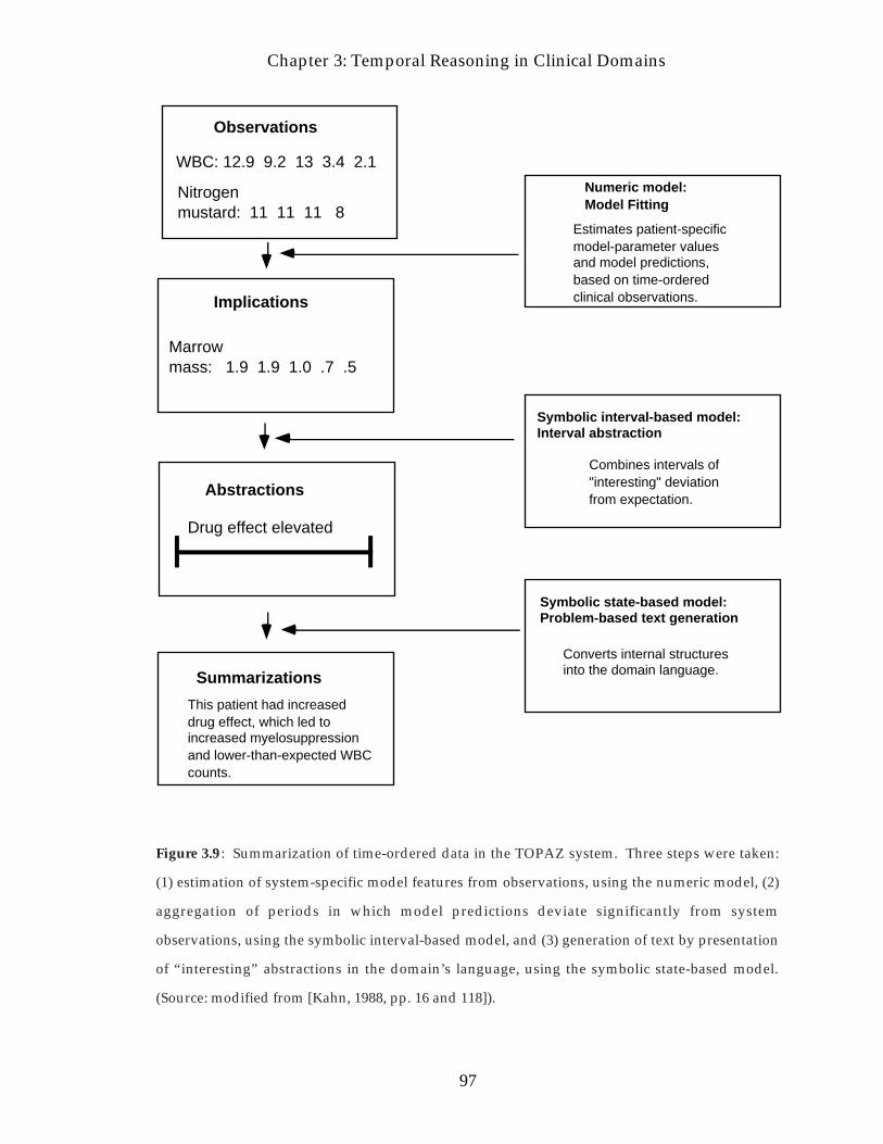
Chapter 3: Temporal Reasoning in Clinical Domains
97
Numeric model:Model Fitting
Estimates patient-specificmodel-parameter valuesand model predictions,based on time-orderedclinical observations.
Symbolic interval-based model:Interval abstraction
Combines intervals of"interesting" deviationfrom expectation.
Symbolic state-based model:Problem-based text generation
Converts internal structuresinto the domain language.
Observations
WBC: 12.9 9.2 13 3.4 2.1
Nitrogenmustard: 11 11 11 8
Implications
Abstractions
Marrowmass: 1.9 1.9 1.0 .7 .5
Drug effect elevated
Summarizations
This patient had increaseddrug effect, which led toincreased myelosuppressionand lower-than-expected WBCcounts.
Figure 3.9 : Summarization of time-ordered data in the TOPAZ system. Three steps were taken:
(1) estimation of system-specific model features from observations, using the numeric model, (2)
aggregation of periods in which model predictions deviate significantly from system
observations, using the symbolic interval-based model, and (3) generation of text by presentation
of “interesting” abstractions in the domain’s language, using the symbolic state-based model.
(Source: modified from [Kahn, 1988, pp. 16 and 118]).

Chapter 3: Temporal Reasoning in Clinical Domains
98
atemporal patient-specific model were adjusted to fit actual patient-specific
data that accumulate over time (such as response to previous therapy),
turning the model into a patient-specific temporal model [Kahn, 1988].
2. A symbolic interval-based model aggregated intervals that were clinically
interesting in the sense that they violated expectations. The model
encoded abstractions as a hierarchy of symbolic intervals. The symbolic
model created these intervals by comparing population-based model
predictions to patient-specific predictions (to detect surprising
observations), by comparing population-based model parameters to
patient-specific parameter estimates (for explanation purposes), or by
comparing actual patient observations to the expected patient-specific
predictions (for purposes of critiquing the numeric model). The
abstraction step was implemented by context-specific rules.
3. A symbolic state-based model generated text paragraphs that used the
domain’s language, from the interval-based abstractions, using a
representation based on augmented transition networks (ATNs). An
ATN is an enhanced, hierarchical version of a finite-state automaton,
which moves from state to state based on the input to the current state.
An arc leading from state to state can contain actions to be executed when
the arc is traversed. The ATNs encoded the possible summary statements
as a network of potential interesting states. The state model transformed
interval-based abstractions into text paragraphs.
In addition, Kahn [1991b] designed a temporal-maintenance system, TNET, to
maintain relationships among intervals in related contexts and an associated
temporal query language, TQuery [1991d]. TNET and TQuery were used in the
context of the ONCOCIN project [Tu et al., 1989] to assist physicians who were
treating cancer patients enrolled in experimental clinical protocols. The TNET
system was extended to the ETNET system , which was used in the TOPAZ
system. ETNET [Kahn, 1991b] extended the temporal-representation capabilities
of TNET while simplifying the latter’s structure. In addition, ETNET had the

Chapter 3: Temporal Reasoning in Clinical Domains
99
ability to associate interpretation methods with ETNET intervals; such intervals
represented contexts of interest, such as a period of lower-than-expected
granulocyte counts. ETNET was not only a temporal-reasoning system, but also a
flexible temporal-maintenance system. Kahn noted, however, that ETNET could
not replace a database-management system, and suggested implementing it on
top of one [Kahn, 1988].
TOPAZ used different formalisms to represent different aspects of the complex
interpretation task. In that respect, it was similar to the HF program and to the
digitalis therapy advisor. TOPAZ represents a landmark attempt to create a
hybrid interpretation system for time-oriented data, comprising three different,
integrated, temporal models.
The numeric model used for representation of the prototypical (population-
based) patient model, for generation of the atemporal patient-specific model, and
for fitting the calculated parameters with the observed time-stamped
observations (thus adjusting the model to a temporal patient-specific model), was
a complex one. It was also was highly dependent on the domain and on the task
at hand. In particular, the developer created a complex model just for predicting
one parameter (granulocytes) by modeling one anatomical site (the bone marrow)
for patients who had one disease (Hodgkin’s lymphoma) and who were receiving
treatment by one particular form of chemotherapy (MOPP , a clinical protocol that
administers nitrogen mustard, vincristine, procarbazine, and prednisone). Even
given these considerable restrictions, the model encoded multiple simplifications.
For instance, all the drugs were combined into a pseudodrug to represent more
simply a combined myelosupressive (bone-marrow–toxicity) effect. The model
represents the decay of the drug’s effect , rather than the decay of the actual drug
metabolites [Kahn, 1988]. This modeling simplification was introduced because
the two main drugs specifically toxic to the bone-marrow target organ had
similar myelosuppressive effects. As Kahn notes, this assumption might not be
appropriate even for other MOPP toxicity types for the same patients and the
same protocols; it certainly might not hold for other cancer-therapy protocols, or
in other protocol-therapy domains [Kahn, 1988, p. 143]. In fact, it is not clear how

Chapter 3: Temporal Reasoning in Clinical Domains
100
we would adjust the model to fit even the rather related domain of treatment of
chronic GVHD patients (see Section 1.1). Chronic GVHD patients suffer from
similar—but not quite the same—effects due to myelosuppressive drug therapy,
as well as from multiple-organ (e.g., skin and liver) involvement due to the
chronic GVHD disease itself; such effects might complicate the interpretation of
other drug toxicities.
In addition, many clinical domains seem to defy complete numeric modeling.
For instance, the domain of monitoring children’s growth. Similarly, in many
other clinical domains, the parameter associations are well known, but the
underlying physiology and pathology are little or incompletely understood, and
cannot be modeled with any reasonable accuracy.
Even if a designer does embark on modeling, it not obvious when she should stop
modeling. Kahn [1988] cites examples in which adding another component to his
bone-marrow compartment model, thereby apparently improving it, generated
intolerable instability. Similar effects were introduced when the model was
adjusted to rely on more recent laboratory results, thus downplaying the weight
of old data. Another disturbing issue was that spurious results can have a
significant affect in the wrong direction on such a model, but if the model-fitting
procedure is built so as to ignore aberrant data until a clear pattern is established,
the fitting procedure might not be able to detect changes in the patient-specific
parameters themselves—that is, changes in the underlying model. Failing to
detect a changing patient model might be problematic if we were to rely
completely on the model in data-poor domains, such as for the task of managing
patients enrolled in clinical protocols, in which measurements are taken
approximately each week or each month. The problem would be even more
serious in the domain of monitoring children’s growth, where measurements
often include just three or four data points, taken at 1- to 3-year intervals.
Yet another issue in fitting data to a model is the credit-assignment problem:
Just which parameter should be corrected when the model does not fit the
observations? If, in fact, the responsible parameter is not included in the model,

Chapter 3: Temporal Reasoning in Clinical Domains
101
the model’s parameters might be adjusted erroneously to fit the particular data
up to the present time, actually reducing the model’s predictive abilities.
TOPAZ used the patient-specific predictions, not the actual observed data, for
comparisons to the expected population data. The reason for this choice was that
data produced for patient-specific predictions (assuming a correct, complete,
patient-specific model) should be smoother than actual data and should contain
fewer spurious values. However, using predictions rather than observed data
might make it more difficult to detect changes in patient parameters.
Furthermore, the calculated, patient-specific expected values do not appear in the
generated summary and therefore would not be saved in the patient’s medical
record. It is therefore difficult to produce an explanation to a physician who
might want a justification for the system’s conclusions, at least without a highly
sophisticated text-generating module.
The ETNET system was highly expressive and flexible. It depended, however,
on a model of unambiguous time-stamped observations. This assumption also
was made in Russ’ TCS system and in the RÉSUMÉ system (at least as far as the
input, as opposed to the interpretation, is concerned). In addition, TOPAZ did
not handle well vertical (value) or horizontal (temporal) uncertainty, and, as
Kahn remarks, it is in general difficult to apply statistical techniques to data-poor
domains.
The ETNET algorithm, which depended on the given search dates being within
the context-interval containing the context-specific rule, could not detect events
that were contextually dependent on a parent event, but were either disjoint from
that event (beginning after the causing event) or even partially overlapping with
it [Kahn, 1988]. As I show in Chapters 4 and 5, this problem is solved
automatically in the RÉSUMÉ architecture by the inclusion in the domain model
of dynamic induction relations of context intervals . Using dynamic induction
relations, context intervals are created anywhere in the past or future in response
to the appearance of an inducing event, an abstraction, an abstraction goal, or a
combination of several contemporaneous context intervals that are part of a

Chapter 3: Temporal Reasoning in Clinical Domains
102
SUBCONTEXT semantic relation in the domain’s theory. Context intervals
represent a particular context for interpretation during a certain time interval,
and trigger within their temporal span the necessary abstraction rules. These
rules are independent of the domain, and are parameterized by domain-specific
temporal-abstraction knowledge. Thus, the abstraction rules in RÉSUMÉ (within
the temporal-abstraction mechanisms) are not attached to any particular
interpretation context. Temporal properties of domain-specific parameters are
specialized by different interpretation contexts (in the domain’s ontology). These
properties are accessed using the relevant interpretation context(s); more than
one such context might be in effect during the temporal span of interest.
Nevertheless, the idea of having context-specific rules, even if in only an abstract
sense, as it is used in RÉSUMÉ, certainly bears resemblance to that concept as
expressed in VM and TOPAZ. Interpretation contexts, like the TOPAZ ETNET
context nodes, limit the scope of inference, making it easier to match patterns
within their scope, to store conclusions, and to block the application of
inappropriate inference procedures (e.g., rules appropriate for other
interpretation contexts).
3.2.11 Kohane’s Temporal-Utilities Package (TUP)
Kohane [1986; 1987] has written the general-purpose temporal-utilities package
(TUP) for representing qualitative and quantitative relations among temporal
intervals, and for maintaining and propagating the constraints posed by these
relations through a constraint network of temporal (or any other) intervals. The
use of constraint networks is a general technique for representing and
maintaining a set of objects (called the nodes of the network) such that, between
at least some pairs of nodes, there are links (known as arcs) which represent a
relation that must hold between the two nodes. Updating a constraint network
by setting the values of certain nodes or arcs to be fixed propagates the changes
to all the other nodes and arcs.

Chapter 3: Temporal Reasoning in Clinical Domains
103
Kohane's goal was mainly to represent and reason about the complex, sometimes
vague, relations found in clinical medicine, such as "the onset of jaundice follows
the symptom of nausea within 3 to 5 weeks but before the enzyme-level
elevation." When such relations exist, it might be best not to force the patient or
the physician to provide the decision-support system with accurate,
unambiguous time-stamped data. Instead, it may be useful to store the relation,
and to update it when more information becomes available. Thus, a relation
such as "2 to 4 weeks after the onset of jaundice" might be updated to "3 to 4
weeks after the onset of jaundice" when other constraints are considered or when
additional data, such as enzyme levels, became available. Such a strategy is at
least a partial solution to the issue of horizontal (temporal) uncertainty in clinical
domains, in which vague patient histories and unclear disease evolution patterns
are common.
The TUP system used a point-based temporal ontology. Intervals were
represented implicitly by the relations between their start points and end points,
or by the relations between these points and points belonging to other intervals.
These relations were called range relations (RRELs). A simplified structure of an
RREL is shown in Figure 3.10.
Essentially, Kohane had implemented a point-based strategy for representing
some of Allen's interval-based relations that were discussed in Section 3.1.4—
namely, those that can be expressed solely by constraints between two points.
(RREL <first-point specification> <second-point specification>
<lower-bound distance> <upper-bound distance>
<context>)
Figure 3.10: A range relation (RREL). The RREL constrains the temporal distance between two
points to be between the given lower bound and the upper bound in a certain context. (Source:
modified from [Kohane, 1987, p. 17].)

Chapter 3: Temporal Reasoning in Clinical Domains
104
For instance, to specify that interval A precedes interval B, it is sufficient to
maintain the constraint that "the end of A is between +INFINITY and +ε before the
start of B." This more restricted set of relations is the one discussed by Villain
and Kautz [Villain and Kautz, 1986; Villain et al., 1989], who were mentioned in
Section 3.1.4 as showing that the full Allen interval algebra is computationally
incomplete (in tractable time). The point-based, restricted temporal logic
suggested by Villain and Kautz is computationally sound and complete in
polynomial time, since point-based constraints can be propagated efficiently
through the arcs of the constraint network. However, such a restricted logic
cannot capture disjunctions of the type "interval A is either before or after interval
B,” since no equivalent set of constraints expressed as conjunctions using the end
points of A and B can express such a relation. Whether such relations are needed
often, if at all, in clinical medicine is debatable. I mentioned in Section 3.1.5 that
van Beek formulated a similar restricted algebra (SIA) and implemented several
polynomial algorithms for it [van Beek, 1991]. SIA is based on equality and
inequality relations between points representing interval end points, and
disallows only the strict inequality relation. Using van Beek's SIA algebra and
associated algorithms, we can refer queries to a system of intervals such as is
managed by Kahn's TNET temporal-management system, and get answers in
polynomial time to questions such as, "Is it necessarily true that the patient had a
cycle of chemotherapy that overlapped a cycle of radiotherapy?" Van Beek
claimed that his limited interaction with physician experts suggested that many
domains do not, in fact, need more than the SIA algebra to express temporal
relations [van Beek, 1991]. This simplification, of course, results in considerable
time and space savings, and ensures the user of soundness and completeness in
conclusions involving temporal relations.
Kohane tested the TUP system by designing a simple medical expert system,
temporal-hypothesis reasoning in patient history (THRIPHT). The THRIPHT
system accepted data in the form of RRELs and propagated newly computed
upper and lower bounds on temporal distances throughout the TUP-based
network. The diagnostic, rule-based algorithm (in the domain of hepatitis)

Chapter 3: Temporal Reasoning in Clinical Domains
105
waited until all constraints were propagated, and then queried the TUP system
using temporal predicates such as, "Did the patient use drugs within the past 7
months, starting as least 2 months before the onset of jaundice?" [Kohane, 1987].
The THRIPHT system used the hierarchical diagnostic structure of the MDX
diagnostic system [Chandrasekaran and Mittal, 1983] to limit the contexts in
which it looked for evidence for specific hypotheses. (MDX was an ontology of
diseases designed for the use of a generic classification problem-solving method
[see Section 2.1].)
3.2.12 Haimowitz’s and Kohane’s TrenDx System
A recent system, demonstrating initial encouraging results, is Haimovitz's and
Kohane’s TrenDx temporal pattern-matching system [Haimowitz and Kohane,
1992; Haimowitz and Kohane, 1993a, 1993b; Kohane and Haimowitz, 1993;
Haimowitz, 1994]. The goals of TrenDx do not emphasize the acquisition,
maintenance, reuse, or sharing of knowledge. Moreover, TrenDx does not aim to
answer temporal queries about clinical databases. Instead, it focuses on using
efficient general methods for representing and detecting predefined temporal
patterns in raw time-stamped data.
The TrenDx system uses Kohane’s TUP constraint-network utilities (see Section
3.2.11) to maintain constraints that are defined by temporal trend templates
(TTs). TTs describe typical clinical temporal patterns, such as normal growth
development, or specific types of patterns known to be associated with
functional states or disease states, by representing these patterns as horizontal
(temporal) and vertical (measurement) constraints. The TrenDx system has been
developed mainly within the domain of pediatric growth monitoring, although
hypothetical examples from other domains have been presented to demonstrate
its more general potential [Haimowitz and Kohane, 1993a, 1993b].
A typical TT representing the expected growth of a normal male child is shown
in Figure 3.11. The growth TT declares several predefined events, such as
PUBERTY ONSET; these events are constrained to occur within a predefined

Chapter 3: Temporal Reasoning in Clinical Domains
106
0 2 3 10 13Age (years)
Wt Z-scoreHt Z-score
Ht Z score - Wt Z score
Establish centiles
Birth
Puberty onset
Prepuberty
Figure 3.11: A portion of a trend template (TT) in TrenDx that describes the male average normal
growth as a set of functional and interval-based constraints. All Z scores are for the average
population. The Birth landmark, assumed to denote time 0, is followed by an uncertain period of
2 to 3 years in which the child’s growth percentiles are established, and in which the difference
between the Ht Z score and the Wt Z score are constrained to be constant. During an uncertain
period of prepuberty ending in the puberty onset landmark sometime between the age of 10 and
13, the Ht Z score and the Wt Z score are both constrained to be constant. = landmark or
transition point; = constant value indicator; Ht = height; Wt = weight; Z score indicates
number of standard deviations from the mean. (Source: adapted from [Haimowitz, 1994, p. 45]).
temporal range: For instance, PUBERTY ONSET must occur within 10 to 15 years
after birth. Within that temporal range, height should vary only by ±δ.
In general, a TT has a set of value constraints of the form m ≤ f(D) ≤ M, where m
and M are the minimum and maximum values of the function f defined over the
measurable parameters D in the temporal range of the interval.
TrenDx has the ability to match partial patterns by maintaining an agenda of
candidate patterns that possibly match an evolving pattern. Thus, even if TrenDx
gets only one point as input, it might (at least in theory) still be able to return a
few possible patterns as output. As more data points are known, the list of
potential matching patterns and their particular instantiation in the data is

Chapter 3: Temporal Reasoning in Clinical Domains
107
modified. This continuous pattern-matching process might be considered a goal-
directed approach to pattern matching, contrasting with the RÉSUMÉ approach
of first generating meaningful basic abstractions (that were considered important
by the expert for the particular context in question), then using a simpler pattern-
matching mechanism to retrieve arbitrary patterns.
TrenDx has been tested in a clinical trial on a small number of patients; its
conclusions agreed partially with a three-expert panel on the appropriate
diagnosis [Haimovitz and Kohane, 1993a].
The design of the TrenDx system is quite different from that of other systems
described in this chapter, reflecting different goals. TrenDx does not have a
knowledge base in the sense of the IDEFIX medical knowledge base or the
RÉSUMÉ parameter, event, and context ontologies; thus, many TTs, or parts of
TTs, will have to be reconstructed for new tasks in the same domain that rely on
the same implicit knowledge. In the case of TrenDx, this knowledge is encoded
functionally in the set of value constraints that serve as lower and upper bounds
for, essentially, black-box functions. The lack of a distinct knowledge base means
that TrenDx does not represent explicitly that a construct that appears in several
TTs, such as “the allowed function f(D) values are within ±δ” might play the
same knowledge role (see Chapter 2) in many TTs—namely, the allowed
significant deviation of that parameter in that context, such as might be useful for
recognizing a DECREASING trend. Furthermore, even if the same parameter
appeared in a somewhat different TT using the same implicit significant-
deviation concept (with the same function f and even with the same δ), the
designer of the new TT would have to specify both f and δ repeatedly.
Since TrenDx does not have a hierarchical parameter knowledge base, it cannot
inherit knowledge about, for instance, the Hb parameter, the parameter’s
ALLOWED RANGE value, or its DECREASING properties, from any other context
involving Hb. In particular, TrenDx cannot inherit a top-level context that
defines the basic properties of Hb in any context, such as in the IDEFIX medical
knowledge base or in the RÉSUMÉ ontology. An additional implication of the

Chapter 3: Temporal Reasoning in Clinical Domains
108
lack of an explicit knowledge base would be a difficulty in representing basic
qualitative relationships for all contexts, whereas the HF program, TOPAZ, and
RÉSUMÉ (to some extent) can. Therefore, acquiring a set of new TTs, even for the
same clinical domain, might involve redefining implicitly many functions, value
constraints, units of measurement, partial trends, and so on, that in fact play the same
knowledge roles in previously acquired TTs. It might therefore be quite difficult to
support the design of a new TT by a domain expert, since that design might
involve the equivalent of a significant amount of low-level programming.
As I have mentioned, TrenDx has different goals compared to systems such as
Downs’ medical-record summarization program, IDEFIX, TOPAZ, and
RÉSUMÉ. TrenDx does not form intermediate-level abstractions (such as
DECREASING(HB)), save them, or maintain logical dependencies among them
(e.g., by a truth-maintenance system) as RÉSUMÉ or TCS do. Instead, TrenDx
tries to match in the input data a predefined set of templates. TrenDx does not
answer arbitrary temporal queries at various intermediate abstraction levels (e.g.,
“was there any period of a DECREASING standard-deviation score of the height
parameter for more than 2 years?”). TrenDx assumes that all the interesting
queries in the domain had been defined as TTs, and that no new queries will be
asked by the user during runtime.
Due to the different design, TrenDx cannot answer queries regarding an
intermediate-level concept (such as bone-marrow toxicity levels), even if the
answer has been part of its input (e.g., the physician might have recorded in the
chart that the patient has bone-marrow toxicity grade III). The reason is that TTs
are defined in terms of only the lowest-level input concepts (e.g., height, weight,
Hb-level values). This limitation does not exist in systems such as IDEFIX,
TOPAZ, and RÉSUMÉ.
Note also that the lack of intermediate abstractions might pose grave difficulties
in acquiring complex new patterns, since the TrenDx patterns seem much more
complex than are the typical high-level queries presented to Kahn’s TQuery
interpreter or to RÉSUMÉ’s query mechanism: The TTs essentially encapsulate
Chapter 3: Temporal Reasoning in Clinical Domains
109
all levels of abstraction at once, and all would have to be captured (and
redefined) in the pattern.
RÉSUMÉ, consequently, has different, more general, goals: Representation of
temporal-abstraction knowledge in a domain-independent, uniform manner,
such that the problem-solving knowledge might be reusable in other domains
and that the domain knowledge be sharable among different tasks. In addition,
one of the goals in RÉSUMÉ is to formalize and parameterize temporal-
abstraction knowledge so that it can be acquired directly from a domain expert
using automated KA tools (see Chapter 6). This desire for uniformity and
declarative form in the representation scheme, and the fact that either the
available input or the requested output might be at various intermediate (but
meaningful) levels of abstraction, influenced my decision to avoid domain-
specific patterns using low-level input data as the sole knowledge
representation5.
Although their goals are different, RÉSUMÉ and TrenDx are similar in at least
one sense: They assume incomplete information about the domain, which
prevents the designer from building a complete model and simulating that
model to get more accurate approximations. Thus, both systems use
associational patterns, albeit in a different manner, that fit well domains in which
the underlying pathophysiological model cannot be captured completely by a
mathematical model, and, in particular, domains in which data are sparse.
3.2.13 Larizza's Temporal-Abstraction Module in the M-HTP System
M-HTP [Larizza, 1990; Larizza et al., 1992] is a system devoted to the abstraction
of time-stamped clinical data. In the M-HTP project, Larizza constructed a
system to abstract parameters over time for a program monitoring heart-
5The initial goal and the tools used to construct these two systems also might explain some of thedesign differences. For instance, TrenDx is built on top of a constraint-propagation network, theTUP system, and naturally defines patterns as constraints. TrenDx also assumes that the top-level, final diagnosis is the main goal, implying a goal-driven control strategy, while one of thereasons for the mainly (but not only) data-driven control in RÉSUMÉ is the desire to generate allrelevant intermediate-level abstractions.

Chapter 3: Temporal Reasoning in Clinical Domains
110
transplant patients. The M-HTP system generates abstractions such as HB-
DECREASING, and maintains a temporal network (TN) of temporal intervals,
using a design inspired by Kahn’s TNET temporal-maintenance system (see
Section 3.2.10) [Larizza et al., 1992]. Like TNET, M-HTP uses an object-oriented
visit taxonomy (Figure 3.12) and indexes parameters by visits.
M-HTP also has an object-oriented knowledge base that defines a taxonomy of
significant-episodes—clinically interesting concepts such as DIARRHEA or
WBC_DECREASE. Parameter instances can have properties, such as MINIMUM (see
Figure 3.13). The M-HTP output includes intervals from the patient TN that can
be represented and examined graphically, such as “CMV_viremia_increase”
during particular dates [Larizza et al., 1992].
Visits
Date_dd_mm_yy = unknown
Day_since_transplantation = unknown
Visit_date = unknown
Visit_hour = unknown
Visit_number = unknown
Date_dd_mm_yy = 12 Dec 1990
Day_since_transplantation = 37
Visit_date = 90/12/12
Visit_hour = 11:00
Visit_number = 14
(+)Visit 14
(+)WBC14
(+)EA14
(+)Antiviral14
(+)IEA14
(+)cya_dose14
Date_dd_mm_yy = 12 Dec 1990
Day_since_transplantation = 37
Visit_date = 90/12/12
Symbolic_value = mild_leukopenia
Visit_number = 14
(+)Visit2
(+)Visit10
Numeric_value = 14
(+)Visit13
(+)Visit15
(+)Visit7
(+)Visit1
Figure 3.12 : A portion of the M-HTP visits taxonomy. Clinical-parameter values are indexed by
visits. Visits are aggregates of all data collected in the same day. = class; ∆ = object; = slot.
(Source: modified from [Larizza et al., 1992, p. 119].)

Chapter 3: Temporal Reasoning in Clinical Domains
111
Clinical_contexts Significant_episodes
WBC_decrease
Fever_episodes
Diarrhea
CMV_viremia_increase
CMV_antigenemia_increase
Gastric_pain
cya_level_decrease
cya_level_increase
immunosuppresion
Average
Duration
End_date
First_visit
Granularity
Last_visit
Left_bound
Maximum
Minimum
Pattern
Right_bound
St_deviation
Start_date
Figure 3.13 : A portion of the M-HTP significant episodes taxonomy. Each significant episode has
multiple attributes. = class; = slot. (Source: modified from [Larizza et al., 1992, Page
120].)
The temporal model of the M-HTP system includes both time points and
intervals. The M-HTP system uses a temporal query language to define the
antecedent part of its rules, such as “an episode of decrease in platelet count that
overlaps an episode of decrease of WBC count at least for 3 days during the past
week implies suspicion of CMV infection” [Larizza et al., 1992].
The M-HTP system can be viewed as a particular, domain-specific instance of the
RÉSUMÉ system. There is no indication that the M-HTP system is easily
generalizable for different domains and tasks. For instance, concepts such as
WBC_DECREASE are hard-coded into the system (see Figure 3.13). As I show in
Chapter 5, this hardcoding is conceptually different from the RÉSUMÉ system’s

Chapter 3: Temporal Reasoning in Clinical Domains
112
representation of knowledge about several domain-independent abstraction
classes (states, gradients, rates and patterns). For instance, in RÉSUMÉ, the
gradient-abstractions class contains knowledge about abstracting gradients.
Particular domains can have domain-specific subclasses, such as
WBC_GRADIENT. In a gradient subclass, a particular value (e.g., one of the
default values DECREASING, INCREASING, SAME and so on), and its inference
properties can be inherited from the gradient abstractions class, and can be used
by all instances of the gradient subclass.
In the M-HTP system, there is no obvious separation between domain-
independent abstraction knowledge and domain-specific temporal-reasoning
properties. In an example of the patient TN [Larizza], we can find the class
SIGNIFICANT EPISODES, which presumably includes knowledge about clinical
episodes, subclasses of that class (e.g., WBC_DECREASE), and instances of the
latter subclass (e.g., WBC_DECREASE_1), that presumably denote particular
instances of patient data. This situation is not unlike that in Downs’ program
(see Section 6.2.6), which influenced de Zegher-Geets’ definition of a separate
medical knowledge base. Note also that a slot such as the MINIMUM VALUE of a
parameter does not define a new abstraction class, such as are state abstractions
in RÉSUMÉ: It is a function from the values of a particular instance into the values
of the same instance (e.g., into the potential Hb levels—say, 7.4 gr./dl Hb), rather
than into the range of values of a new class—namely the state abstractions of Hb
(e.g., possible state values—say, LOW). Abstraction classes, including patterns,
are thus not first-class parameters in the M-HTP system (unlike their status in the
RÉSUMÉ model), and cannot be described using the full expressive capacity of a
language that might describe properties of parameters (e.g., the scale—say,
ORDINAL).
RÉSUMÉ can therefore be viewed as a metatool for a representation of the
temporal-abstraction knowledge of M-HTP. The representation would use
RÉSUMÉ’s domain-independent (but task-specific) language. As I show in
Chapter 6, most of that knowledge can be acquired in a disciplined manner,

Chapter 3: Temporal Reasoning in Clinical Domains
113
driven by the knowledge roles defined by the temporal-abstraction mechanisms
that solve the tasks posed by the knowledge-based temporal-abstraction method.
3.3 Discussion
Each of the approaches used to solve the temporal-abstraction task in clinical
domains has various features, advantages, and disadvantages. In presenting
these approaches, I have pointed out some of these features, and have discussed
these features with respect to comparable aspects in the RÉSUMÉ system's
methodology. It is clear that most of the systems presented had different
philosophical and practical goals, and it is therefore difficult to evaluate them in
any real sense, except for pointing out the outstanding features relevant to the
task of temporal reasoning.
Many systems used for monitoring, diagnosis, or planning, employ temporal
reasoning, although that subject is not the main focus of the research. A major
example of such a framework in the clinical domain is the Guardian architecture
for monitoring intensive-care unit patients and for suggesting therapeutic actions
for these patients [Hayes-Roth et al., 1992]. In Guardian, a distinction is made
among intended, expected and observed parameter values. Values have temporal
scopes. Thus, arterial oxygen pressure might have a desirable intended range of
values; a suggested correction in an external variable might be expected to
produce within 1 minute a certain value in the patient’s measured parameter;
and a particular observation, 2 minutes later, might return a value quite different
from either of these, thus suggesting some type of a problem. The time-stamped
input data is preprocessed using a set of parameter-specific filters that initiate, in
effect, the abstraction process [Washington and Hayes-Roth, 1989]. A Fuzzy-
logic system based on trasholding sigmoidal functions is used in order to detect
temporal patterns ([Drakopoulus and Hayes-Roth, 1994]; see also Section 8.4.4).
Although most of the systems I have discussed in Section 3.2 seem, on the
surface, to be solving an interpretation task in a temporal domain, we have to
distinguish systems that summarize patient data over time (e.g., Downs’
program, IDEFIX, TOPAZ, M-HTP, and RÉSUMÉ), and answer random or

Chapter 3: Temporal Reasoning in Clinical Domains
114
structured queries about their interpretations (e.g., TOPAZ and RÉSUMÉ) from
systems that try to generate final diagnoses from low-level data (e.g., TrenDx). A
closely related issue is whether the system attempts to perform a temporal
management function, in addition to the temporal reasoning one (e.g., TOPAZ and
M-HTP). An extreme case is Russ’s TCS system, which did not perform any
domain-dependent temporal reasoning, although it performed a considerable
amount of domain-independent temporal-management work behind the scenes
to ensure that the user could effectively not worry about time. Thus, TCS could
be considered a temporal-reasoning–support system. We also should make a
distinction between systems whose implicit or explicit summarization goal is just
a subgoal of another task, such as treating patients (e.g., VM) or predicting the
next state of the monitored system (e.g., the HF program), and systems whose
major purpose is to summarize the patient’s record (e.g., IDEFIX and RÉSUMÉ)
or at least to detect significant temporal or causal trends in that record (e.g., Rx).
Other distinctions can be made, since no two systems are alike.
Nevertheless, most of the systems I have discussed—at least those that needed to
perform a significant amount of the temporal-abstraction task—in fact solved
tasks closely related to the five tasks that I presented in Section 1.1 as the
fundamental subtasks of the temporal-abstraction task. Recall that the temporal-
abstraction task is explicitly decomposed into these five subtasks by the
knowledge-based temporal-abstraction method (see Figure 1.2). Furthermore,
the systems that I have described often relied implicitly on the four types of
temporal-abstraction knowledge I defined: structural knowledge, classification
knowledge, temporal-semantic knowledge, and temporal-dynamic knowledge.
This knowledge, however, often was not represented declaratively, if at all. For
instance, all systems described had to solve the context-restriction task before
interpretation could proceed and therefore created various versions of
interpretation contexts (e.g., the intervals created by TOPAZ and the TN module
of M-HTP, the external states determined by the state-detection rules of VM, and
the steady states partitioned by TCS). There was always a classification task (e.g.,
determining severity levels by IDEFIX, or creating interval-based abstraction

Chapter 3: Temporal Reasoning in Clinical Domains
115
from numeric patient-specific and population-dependent data). There was
always the need to create intervals explicitly or implicitly, and thus to reason
about local and global change (e.g., Downs’ program used temporal predicates,
IDEFIX defined TOPFs, and Rx required a library of time-dependent database
access functions). All systems assumed implicitly some model of proposition
semantics over time—for instance, allowing or disallowing automatic
concatenation of contexts and interpretations (VM, IDEFIX). Finally, all systems
eventually performed temporal pattern matching, explicitly (e.g., TOPAZ, using
ETNET) or implicitly (e.g. Downs’ temporal predicates, which were also used in
IDEFIX as input to the odds-likelihood update function, and the TrenDx pattern-
matching algorithm, using the low-level constraints). In addition to the task
solved, there were common issues to be resolved inherent in maintaining the
validity of a historic database (e.g., Russ’s TCS system and RÉSUMÉ use a truth-
maintenance system).
The knowledge-based temporal-abstraction method makes explicit the subtasks
that need to be solved for most of the variations of the temporal-abstraction
interpretation task. These subtasks have to be addressed, explicitly or implicitly,
by any system whose goal is to generate interval-based abstractions. The
temporal-abstraction mechanisms that I have chosen to solve these subtasks
make explicit both the tasks they solve and the knowledge that they require to
solve these tasks.
None of the approaches that I have described focuses on the knowledge-
acquisition, knowledge-maintenance, knowledge-reuse, or knowledge-sharing
aspects of designing and building large knowledge-based medical systems. In
other words, the approaches described, as applied to the temporal-abstraction
task, were not represented at the knowledge level. We might therefore expect these
approaches to be plagued by most of the design and maintenance problems of
knowledge-based systems that were discussed in Chapter 2. In particular, we
would expect difficulties when we attempt (1) to apply these approaches to
similar tasks in new domains, (2) to reuse them for new tasks in the same
domain, (3) to maintain the soundness and completeness of their associated

Chapter 3: Temporal Reasoning in Clinical Domains
116
knowledge base and its interrelated components, and (4) to acquire the
knowledge required to instantiate them in a particular domain and task in a
disciplined and perhaps even automated manner.
In Chapter 4, I present a knowledge-level view of the knowledge-based
temporal-abstraction method and its mechanisms, designed precisely so that
such limitations might be removed or their burden be lessened. I present a
unified, explicit framework for solving the temporal-abstraction task by (1)
defining formally the ontology of the temporal-abstraction task assumed by the
knowledge-based temporal-abstraction method, namely, the domain entities
involved and their relationships, (2) defining the subtasks into which the
temporal-abstraction task is decomposed by the knowledge-based temporal-
abstraction method; (3) defining formal mechanisms that can be used to solve
these subtasks; and (4) pointing out the domain-specific knowledge roles used in
these mechanisms, their explicit nature, semantics, and interrelationships, and
the way they can be organized and used to solve the temporal-abstraction task.

Chapter 4: Knowledge-Based Temporal Abstraction
117
4 Knowledge-Based TemporalAbstraction
In Chapter 1, I gave several examples of the temporal-abstraction task (see Figure
1.1.), and I presented an overview of the knowledge-based temporal-abstraction
method (see Figure 1.2). This method decomposes the temporal-abstraction task
into five subtasks , and solves these five subtasks using five knowledge-based
temporal-abstraction mechanisms . As I have shown in Section 3.2, some or all of
the five subtasks had been in fact implicit goals for every system that has
attempted to solve the temporal-abstraction task in clinical domains, and are thus
very general. (In theory, the knowledge engineer that designs a temporal-
abstraction system for a new domain might select mechanisms other than the
ones that I am suggesting to solve one or more of the five subtasks posed by the
knowledge-based temporal-abstraction method, such as the task of forming
contexts, as long as the input and output semantic constraints of these subtasks
are satisfied). The knowledge-based temporal-abstraction mechanisms I suggest
rely in turn on four domain-specific knowledge types. These four types of
knowledge constitute the only interface between the knowledge-based temporal-
abstraction method and the knowledge engineer who is using that method.
Thus, the development of a temporal-abstraction system particular to a new
domain relies on only the creation or editing of a predefined set of four
knowledge categories, most of which are purely declarative. These knowledge
categories need to be acquired, manually or in an automated fashion, from a
domain expert (e.g., an expert physician).
In this chapter, I present a detailed knowledge-level view (see Section 2.1) of the
knowledge-based temporal-abstraction method and of the five temporal-
abstraction mechanisms that I suggest for solving the five subtasks that method
poses. I define precisely the nature of the four types of domain-specific
temporal-abstraction knowledge, and the roles (see Section 2.1) that these four
types play in the five mechanisms. In Chapter 5, I describe a particular

Chapter 4: Knowledge-Based Temporal Abstraction
118
implementation of the five temporal-abstraction mechanisms and the knowledge
they rely on (i.e., the RÉSUMÉ system). The RÉSUMÉ system demonstrates
additional design concepts important for a discussion of the knowledge-based
temporal-abstraction method as an appropriate solution for the temporal-
abstraction task. In particular, I discuss several issues pertaining to the
appropriate organization and representation of the temporal-abstraction
knowledge. I also discuss several computational issues, such as control methods
and the handling of nonmonotonicity.
To describe the working of the knowledge-based temporal-abstraction method
and mechanisms, I start by defining a formal model of the temporal abstraction
task as that task is solved by the knowledge-based temporal-abstraction method.
The formal model will enable us to define clearly the inputs and outputs to the
five subtasks defined by that method and to the five mechanisms solving,
respectively, these subtasks. I then describe each of the five temporal-abstraction
mechanisms, the task that each mechanism solves, and the formal specifications
of its knowledge requirements. Since the mechanisms create abstractions that
might change as more data arrive, I discuss (in Section 4.2.6) the nonmonotonic
nature of the conclusions output by the five mechanisms. Finally, I summarize
the model and evaluate its main features. The model of temporal abstraction, the
knowledge types of which this model is constructed, and the inferences that this
model permits, together define a knowledge-based temporal-abstraction theory.
The reader might find that the description in Chapter 3 of general temporal
models and of particular clinical temporal-reasoning systems is helpful (although
not absolutely necessary) when reading this chapter, since at times I compare the
temporal-abstraction model and its implied inference framework to other
approaches.
4.1 The Temporal-Abstraction Ontology
The knowledge-based temporal-abstraction method, and the five temporal-
abstraction mechanisms solving the five subtasks posed by that method when it
solves the temporal-abstraction task, make several assumptions with respect to

Chapter 4: Knowledge-Based Temporal Abstraction
119
the underlying temporal model of the domain. In particular, they assume a
certain structure of time and of propositions that can be interpreted over time.
Thus, the temporal-abstraction mechanisms assume a task-specific ontology (i.e.,
a theory of what entities, relations, and properties exist, at least in a particular
domain) for temporal abstraction. My intention in this section is to define an
ontology of events (e.g., drug administrations), an ontology of parameters (e.g.,
blood-glucose value), an ontology of interpretation contexts within which
parameters will be interpreted and abstracted into higher-level concepts, and the
relations among these ontologies. I will then use these ontologies to formally
define the temporal-abstraction task that the knowldge-based temporal-
abstraction method is solving.
Informally, the temporal model that I use includes both time intervals and time
points . The points are the basic temporal primitives, but propositions, such as
occurence of events and existence of parameter values, can be interpreted only
over time intervals. All propositions are therefore fluents [McCarthy and Hayes,
1969]; that is, they must be interpreted over a particular time period (e.g., the
value of the Temperature parameter at time [t, t]).
The various types of entities and propositions that I define can be seen as logical
sorts. I will usually clarify immediately which set of symbols denotes each sort;
thus, the notation “a parameter π ∈ Π ” means that each individual parameter,
denoted by π, will be a member of a new set of symbols Π (denoting only
parameters). Other conventions are used; for instance, relation names are
denoted by small capital letters. The List of Symbols in the preamble to this
dissertation lists all the symbols and conventions I use; the reader might use it as
a glossary.
The temporal-abstraction model comprises the following set of entities:
1. The basic time primitives are time stamps, T i ∈ T. Time stamps are
structures (e.g., dates) that can be mapped, by a time-standardization
function fs(Ti), into an integer amount of any element of a set of
predefined temporal granularity units Gi ∈ Γ (e.g., DAY). A zero-point

Chapter 4: Knowledge-Based Temporal Abstraction
120
time stamp must exist, with relationship to which the time stamps are
measured in the G i units. (Intuitively, the 0 point might be grounded in
each domain to different absolute, “real-world,” time points: the patient’s
age, the start of the therapy, the first day of the 20th century.) The domain
must have a time unit G0 of the lowest granularity (e.g., SECOND), similar
to the chronons defined by Clifford [1988] (see Section 3.1.7); there must
exist a mapping from any integer amount of granularity units G i into an
integer amount of G0. A finite negative or positive integer amount of Gi
units is a time measure .
(Intuitively, time stamps might be represented using units such as days,
hours, or seconds, or at any finite granularity level. However, such time
units must be convertible to the lowest granularity level of the domain.
The lowest granularity level actually used is a task-specific choice; for
instance, in the domain of monitoring children’s growth, a reasonable
granularity unit might be MONTH).
The special symbols +∞ and -∞ are both time stamps and time measures,
denoting the furthest future and the most remote past, respectively. Any
two time stamps must belong to either a precedence relation or an
equivalence relation defined on the set of pairs of time stamps. The
precedence relation is areflexive, antisymmetric, and transitive, intuitively
corresponding to a temporal order, while the equivalence relation denotes
temporal equivalence, at least for the domain at hand. The -∞ time stamp
precedes any other time stamp; the +∞ time stamp follows (is preceded
by) all other time stamps. In addition, the operation of subtracting any
two time stamps from each other must be defined and should return as a
result a time measure, including +∞ or -∞. Finally, the operation of
adding or subtracting a time measure to or from a time stamp must return
a time stamp.
Time stamps resemble the result of applying a date function to
McDermott’s states [McDermott, 1982], which I described in Section 3.1.5.

Chapter 4: Knowledge-Based Temporal Abstraction
121
However, McDermott maps states (snapshots of the world) to the real-
numbers line. The discreteness of time stamps is necessitated by the
nature of the temporal-abstraction task (i.e., interpretation), and of that
task’s input (i.e., time-stamped data). The temporal-abstraction
mechanisms are quite general, however, and do not rely on that
discreteness. The temporal-abstraction mechanisms do depend on the
unambiguousness inherent in time stamps, on the existence of the
temporal precedence and equivalence relations, and on the computational
properties defined above. Temporal uncertainty is therefore modeled by
the nature of the processing of time-stamped data, but is not modeled by
the time stamps themselves.
2. A time interval I is an ordered pair of time stamps representing the
interval’s end points: [I.start, I.end]. Time points Ti are therefore
represented as zero-length intervals where I .start = I.end. Propositions
can only be interpreted over time intervals.
As will be clear from the rest of the definitions of the temporal-abstraction
ontology, the set of points included in a time interval depends on the
proposition interpreted over that interval. A time interval can be closed
on both sides (in the case of state-type and pattern-type parameter
propositions and interpretation contexts), open on both sides (in the case
of gradient- and rate-type abstractions), or closed on the left and open on
the right (in the case of event propositions).
3. An interpretation context ξ ∈ Ξ is a proposition that, intuitively,
represents a state of affairs (e.g., “the drug insulin has an effect on blood
glucose during this interval”). When interpreted over a time interval it
can change the interpretation of one or more parameters within the scope
of that time interval (e.g., of the state of the blood-glucose level, by
suggesting a different definition of the LOW value).
A SUBCONTEXT relation is defined over the set of interpretation contexts.
An interpretation context in conjunction with one of its subcontexts can

Chapter 4: Knowledge-Based Temporal Abstraction
122
create a composite interpretation context. Composite interpretation
contexts are interpretation contexts. Formally, the structure <ξ i, ξj> is an
interpretation context, if the ordered pair (ξj , ξi) belongs to the
SUBCONTEXT relation. In general, if the structure <ξ1, ξ2,...ξ i> is a
(composite) interpretation context, and the ordered pair (ξ j, ξi) belongs to
the SUBCONTEXT relation, then the structure <ξ 1, ξ 2,...ξ i, ξ j> is a
(composite) interpretation context.
Intuitively, composite interpretation contexts allow us to define
increasingly specific contexts (e.g., a specific drug regimen that is a part of
a more general clinical protocol), or combinations of different contexts, for
interpretation of various parameters. Composite interpretation contexts
represent a combination of contemporaneous interpretation contexts whose
conjunction denotes a new context that has some significance in the
domain for the interpretation of one or more parameters.
4. A context interval is a structure <ξ , I>, consisting of an interpretation
context ξ and a temporal interval I.
Intuitively, context intervals represent an interpretation context
interpreted over a time interval; within the scope of that interval, it can
change the interpretation of one or more parameters . Thus, the effects of
chemotherapy form an interpretation context that can hold over several
weeks, within which the ranges of hematological parameters should be
defined differently.
5. An event proposition e ∈ Ε (or an event , for short, when no ambiguity
exists) represents the occurrence of an external volitional action or process
(as opposed to a measurable datum, such as temperature), such as
administering a drug . Events have a series ai of event attributes (e.g.,
dose). Each attribute ai must be mapped to an attribute value νi.
Formally, there exists an IS-A hierarchy (in the usual sense) of event
schemas (or event types). Event schemas have a list of attributes ai, where

Chapter 4: Knowledge-Based Temporal Abstraction
123
each attribute has a domain of possible values Vi, but do not necessarily
contain any corresponding attribute values. Thus, An event proposition is
an event schema in which each attribute ai is mapped to some value νi ∈
Vi. A PART-OF relation is defined over the set of event schemas. If the pair
of event schemas (e i, ej) belongs to the PART-OF relation, then event
schemaei can be a subevent of an event schema e j. (e.g., a CLINICAL
PROTOCOL event can have several parts, all of them MEDICATION events).
6. An event interval is a structure <e , I>, consisting of an event proposition e
and a time interval I .
Intuitively, e is an event proposition (with a list of attribute–value pairs),
and I is a time interval over which the event proposition e is interpreted.
The time interval represents the duration of the event.
7. A parameter schema (or a parameter, for short)π ∈ Π is, intuitively, a
measureable aspect or a describable state of the world (in particular, the
patient’s world), such as the patient’s temperature. Parameter schemas
have various properties , such as a domain Vπ of possible symbolic or
numeric values, measurement units, and a measurement scale (which can
be one of NOMINAL, ORDINAL, INTERVAL, or RATIO, corresponding to the
standard distinction in statistics among types of measurement6). Not all
properties need have values in a parameter schema. There is an IS-A
hierarchy (in the usual sense) of parameter schemas. The combination <π,
ξ> of a parameter π and an interpretation context ξ is an extended
parameter schema (or an extended parameter for short). Extended
parameters are parameters. (For instance, blood glucose in the context of
insulin action, or the platelet count in the context of chemotherapy effects.)
6Nominal-scale parameters have values that cannot be ordered (e.g., color). Ordinal-scaleparameters have values that can be ordered, but the intervals among these values are notmeaningful by themselves and are not necessarily equal (e.g., army ranks). Interval-scaleparameters have meaningful, comparable intervals, although a ratio comparison is notnecessarily meaningful (e.g., temperature measured on different temperature scales). Ratio-scaleparameters have, in addition to all of the above, a fixed zero point and therefore a ratiocomparison, such as “twice as tall” is meaningful regardless of the height measurement unit.

Chapter 4: Knowledge-Based Temporal Abstraction
124
Note that an extended parameter can have properties, such as possible
domains of value, that are different from that of the original
(nonextended) parameter (e.g., in a specific context, a parameter might
have a more refined set of possible values). Extended parameters also
have a special property, a value ν ∈ Vπ. Values typically are known only
at runtime.
(I usually denote parameter names by using leading capital letters, and a
particular value of a parameter property by using small capital letters).
Intuitively, parameters denote either input (usually raw) data, or any level
of abstraction of the raw data (up to a whole pattern). For instance, the
Hemoglobin (Hb) level is a parameter, the White-blood–cell (WBC)
count is a parameter, the Temperature level is a parameter, and so is the
Bone-marrow–toxicity level (that is abstracted from, among other
parameters, the Hb parameter).
The combination of a parameter, a parameter value and an interpretation
context, that is, the tuple <π, ν , ξ> (i.e., an extended parameter and a
value) is called a parameter proposition (e.g., the state of Hb has the value
LOW in the context of therapy by the PAZ protocol). A mapping exists
from all parameter propositions and the parameter properties of their
corresponding parameter (or extended parameter) schema into specific
property values.
Parameter properties can be viewed as multiple-argument relations in
which some of the arguments (i.e., a parameter, a context and a value)
denote a parameter proposition. This will be clear when I enumerate the
knowledge requirements of each of the temporal-abstraction mechanisms
that solve, respectively, each of the temporal-abstraction subtasks. Much
of the knowledge about abstraction of higher-level concepts over time
depends on knowledge of particular parameter and parameter proposition
properties, such as persistence over time of a certain parameter with a
certain value within a particular context. As will be seen in Section 4.2,

Chapter 4: Knowledge-Based Temporal Abstraction
125
different temporal-abstraction mechanisms typically require knowledge
about different parameter properties of the same parameter propositions.
These properties will be enumerated, defined, and discussed at length in
Section 4.2.
Primitive parameters are parameters that play the role of raw data in the
particular domain in which the temporal-abstraction task is being solved
and that cannot be inferred by the temporal-abstraction process from any
other parameters (e.g., laboratory measurements). Primitive parameters
can appear in only the input of the temporal-abstraction task.
Abstract parameters are parameters that play the role of intermediate
concepts at various levels of abstraction; these parameters can be part of
the output of the temporal-abstraction task, having been abstracted from
other parameters and events, or they may be given as part of the input
(e.g., the state of Hb is MODERATE_ANEMIA). In the former case, there is an
ABSTRACTED-INTO relationship between the input parameters and some of
the output parameters. Each pair of parameters that belongs to an
ABSTRACTED-INTO relation represents only one abstraction step; that is, the
ABSTRACTED-INTO relation is not transitive. It is also areflexive and
antisymmetric. If the parameter-pair (πi, πj) belongs to the ABSTRACTED-
INTO relation, either both parameter types are abstract or πi is primitive
and πj is abstract. Abstract-parameter propositions are created during the
temporal-abstraction process by all the temporal-abstraction mechanisms
except the context-forming one.
Constant parameters are parameters that are considered atemporal in the
context of the particular interpretation task that is being solved, so that
their values are not expected to be time dependent (e.g., the patient’s
gender, the patient’s address, the patient’s father’s height). There are in
fact only a few, if any, truly constant parameters (including gender).
When I discuss the temporal-inference mechanism and the inferential
properties knowledge it uses in Section 4.2.3, I mention a way to represent

Chapter 4: Knowledge-Based Temporal Abstraction
126
constants as fluents with a particular set of temporal-semantic inferential
properties, thus removing, in effect, the traditional distinction between
temporal and atemporal variables. It is often useful to distinguish
between (1) internal (or runtime) constants , which are specific to the
particular case being interpreted (e.g., to the current patient) and appear in
the runtime input (e.g., the patient’s name, gender, or age), and (2)
external (or static) constants, which are inherent to the overall task, and
are typically prespecified or appear in the domain ontology (e.g.,
population distributions of heights, or the value of the mathematical
constant π).
8. A parameter interval is a tuple <π, ν , ξ, I>, where <π, ν, ξ> is a parameter
proposition and I is a time interval. If I is in fact a time point (i.e., I .start =
I.end) we can also refer to the tuple as a parameter point .
Intuitively, a parameter interval denotes the value ν of parameter π in the
context ξ during time interval I.
Usually, when meaningful, I denote the value of parameter π in the
beginning of interval I1 as I1.start.π, and the value of parameter π in the
end of interval I as I1.end.π, (see Figure 1.1b for an example of intervals
and parameters).
9. Abstraction functions θ ∈ Θ are unary or multiple-argument functions
from one or more parameters to an abstract parameter. The “output”
abstract parameters can have one of several abstraction types (which are
equivalent to the abstracion function used). I distinguish among at least
three basic abstraction types: state, gradient , and rate . (Other abstraction
functions and therefore types, such as acceleration and frequency, can be
added). These abstraction types correspond, respectively, to a
classification (or computational transformation) of the parameter’s value,
the sign of the derivative of the parameter’s value, and the magnitude of
the derivative of the parameter’s value during the interval (e.g., LOW,
DECREASING, and FAST abstractions for the WBC-count parameter). The

Chapter 4: Knowledge-Based Temporal Abstraction
127
state abstraction is always possible, even with qualitative parameters
having only a nominal scale (e.g., different values of the Color parameter
can be mapped into the abstraction D A R K); the gradient and rate
abstractions are meaningful for only those parameters that have at least an
ordinal scale (e.g., ordinal numbers) or an interval scale (e.g.,
temperature), respectively. In practice, the state-, gradient-, and rate-
abstraction types and their compositions (e.g., the gradient of the state of
the parameter’s value) cover most of the numerical and qualitative data in
clinical domains.
In addition, a special type of abstraction function (and type) is pattern:
The abstract parameter is defined as a temporal pattern of several other
parameters (e.g., a QUIESCENT-ONSET pattern of chronic graft-versus-host
disease; see Figure 1.7).
The θ abstraction of a parameter schemaπ is a new parameter schemaθ(π),
that is, a parameter different from any of the arguments of the θ function
(e.g., STATE(Hb), which I usually write as Hb_State). This new parameter
has its own domain of values, measurement scale, and any other possible
properties. It can also be abstracted further (e.g., GRADIENT(STATE(Hb)),
or Hb_State_Gradient). Note that the new parameter typically has
properties (e.g., scale) that are different from those of the one or more
parameters from which it was abstracted.
Statistics such as minimum, maximum, and average value are not abstraction
types in this ontology. Rather, these are functions on parameter values , that
return simply a value of a parameter, possibly during a time interval, often
from the domain of the original parameter (e.g., the minimum Hb value
within a time interval I can be 8.9 gr/dl, a value from the domain of Hb
values), rather than a parameter schema, which can have a new domain of
values (e.g., the Hb_STATE can have the value INCREASING).
10. An abstraction is a parameter interval <π, ν, ξ, I> where π is an abstract
parameter. If I is in fact a time point (i.e., I .start = I .end), we can also refer

Chapter 4: Knowledge-Based Temporal Abstraction
128
to the abstraction as an abstraction point ; otherwise, we can refer to it as
an abstraction interval.
11. An abstraction goal ψ ∈ Ψ is a proposition that denotes a particular goal
or intention that is relevant to the temporal-abstraction task during some
interval (e.g., the goal of monitoring AIDS patients; the goal of analyzing
growth charts; the intention to control a diabetes patient’s blood-glucose
values). Intuitively, an abstraction goal represents the fact that an
intention holds or that a goal should be achieved during the time interval
over which it is interpreted.
12. An abstraction-goal interval is a structure <ψ, I>, where ψ is a task and I
is a temporal interval.
Intuitively, an abstraction-goal interval denotes a temporal-abstraction
goal (e.g., one of certain specific types of diagnosis or therapy) that is
posed (e.g., by the user or by an automated planner) during an interval. A
an abstraction-goal interval is used for creating correct contexts for
interpretation of data.
13. Intuitively, context intervals are inferred dynamically (at runtime) by
certain event, parameter, or abstraction-goal propositions being true over
specific (i.e., known) time intervals. The interpretation contexts
interpreted over these context intervals are said to be induced by these
propositions (e.g., by the event “administration of four units of regular
insulin”). Certain predefined temporal constraints must hold between the
inferred context interval and the time interval over which the inducing
proposition is interpreted. For instance, the effect of regular insulin with
respect to changing the interpretation of blood-glucose values might start
at least 30 minutes after the start of the administering and might end up to
8 hours after the end of that administraction.
Two or more context-forming propositions might induce indirectly a
composite interpretation context, when their corresponding induced context
Chapter 4: Knowledge-Based Temporal Abstraction
129
intervals are contemporaneous, if the interpretation contexts that hold
during these intervals belong to the SUBCONTEXT relation. I discuss
interpretation contexts and further distinctions among them, as part of the
description of the context-forming mechanism, in Section 4.2.1 and in
Section 5.2.
Formally, a dynamic induction relation of a context interval (DIRC) is a
relation over propositions and time measures, in which each member is a
structure of the form <ξ , ϕ, ss , se, es, ee>. The symbol ξ is the interpretation
context that is induced. The symbol ϕ ∈ Ρ is the inducing proposition , an
event, an abstraction-goal, or a parameter proposition. (An event schema
is also allowed, as shorthand for the statement that the relation holds for
any event proposition representing an assignment of values to the event-
schema’s arguments.) Each of the other four symbols is either the
“wildcard” symbol *, or a (positive, negative or infinite) time measure.
A proposition ϕ that is an inducing proposition in at least one DIRC, is
termed a context-forming proposition.
The inference knowledge represented by DIRCs is used by the context-
forming mechanism to infer new context intervals at runtime. Intuitively,
the inducing proposition is assumed, at runtime, to be interpreted over
some time interval I with known end points. The four time measures
denote, respectively, the temporal distance between the start point of I and
the start point of the induced context interval, the distance between the
start point of I and the end point of the induced context interval, the
distance between the end of I and the start point of the context interval,
and the distance between the end point of I and the end point of the
induced context interval (see Figure 4.2). Note that, typically, only two
values are necessary to define the scope of the inferred context interval
(more values might create an inconsistency), so that the rest can be
undefined (i.e., they can be wildcards, that match any time measure), and
that sometimes only one of the values is a finite time measure (e.g., the ee

Chapter 4: Knowledge-Based Temporal Abstraction
130
distance might be +∞). Note also that the resultant context intervals do
not have to span the same temporal scope over which the inducing
proposition is interpreted.
Due to the existence of DIRCs, a proposition such as an event (or an event
schema), for instance, when interpreted over a particular time interval, can
induce at runtime a multiple series of interpretation contexts. Thus, a
therapy event can induce an context interval whose intuitive meaning is
“a toxicity period for hematological paramters is expected from 2 weeks
after the start of therapy until 4 weeks after the end of the therapy,” as
well as a context interval whose intuitive meaning is “kidney
complications of a very particular sort might occur from 6 months after
the end of the therapy until the unspecified (remotest) future.”
I discuss induced interpretation contexts and context intervals further in
Section 4.2.1, and I examine their details when I describe the architecture
of the context-forming mechanism in Section 5.2.
The use of time stamps as primitives, and interpretation of propositions over
intervals, corresponds to the point-based temporal model as developed by
Shoham [Shoham, 1987; Shoham & Goyal, 1988]. In general, I use a reified
representation [Shoham 1987], in which the proposition “the WBC count is
decreasing during interval I1 in the context ξ” is stated formally as True(I1,
DECREASING(WBC_GRADIENT, ξ)), thus separating the temporal component of the
sentence from the atemporal (parameter-proposition) component. For simplicity,
however, I often refer to this proposition as DECREASING(I1, WBC_GRADIENT, ξ)).
I also use simply DECREASING(WBC) as a syntactic abbreviation when no
confusion is likely; it should be read as “the value of the gradient abstraction of
the WBC-count parameter (i.e., the WBC_GRADIENT parameter) is DECREASING
(during the relevant context and over the relevant time interval).”
Chapter 4: Knowledge-Based Temporal Abstraction
131
Given these definitions, I now can clarify exactly which basic propositions exist
in the ontology of the temporal-abstraction problem-solving method I suggest:
abstraction goals, event propositions, parameter propositions, and interpretation
contexts. These fluents are interpreted over time intervals.
The set of all the relevant event schemas and propositions in the domain, their
attributes and subevents, form the domain’s event ontology . The set of all the
potentially relevant contexts and subcontexts of the domain, whatever their
inducing proposition, defines a context ontology for the domain. The set of all
the relevant parameters and parameter propositions in the domain and their
properties form the domain’s parameter ontology . These three ontologies,
together with the set of abstraction-goal propositions and the set of all DIRCs,
define the domain’s temporal-abstraction ontology. In Chapter 5, I discuss
examples of ontologies of events, contexts and parameters in a domain and their
conceptual repreentation.
Finally, I am assuming the existence of a set of temporal queries, expressed in a
predefined temporal-abstraction language that includes constraints on parameter
values and on relations among start- and end-point values among various time-
intervals and context intervals. That is, a temporal query is a set of constraints
over the components of a set of parameter and context intervals. Intuitively, the
temporal-abstraction language is used (1) to define the relationship between a
pattern-type abstract parameter and its defining parameter intervals, and (2) to
ask arbitrary queries about the result of the temporal-abstraction inference
process. The result of such an “external” query regarding the state of the
knowledge base (including the input and the inferred propositions) depends on
the type of the query. The query type can be either (1) a value query, returning a
value for a parameter-proposition fulfilling the rest of the constraints (e.g., Hb =
9.4 mg/dl during some context), (2) a boolean query asking for the existence of a
proposition given the constraints and returning a boolen value (e.g., TRUE), or (3)
a set query returning a set of parameter propositions (e.g., all parameter
propositions that satisfy a given set of constraints).

Chapter 4: Knowledge-Based Temporal Abstraction
132
The temporal-abstraction task solved by the knowledge-based temporal-
asbtraction method is thus the following task: Given at least one abstraction-goal
interval <ψ, I>, a set of event intervals <e j, Ij>, and a set of parameter intervals
<πk, νk, ξk, Ik> (where ξ k might be an empty interpretation context), and the
domain’s temporal-abstraction ontology, produce an interpretation—that is, a
set of context intervals <ξ n, In> and a set of (new) abstractions <πm,νm, ξm, Im>
(see Figure 1.1), such that the interpretation can answer any temporal query
about all the abstractions derivable from the transitive closure of the input data
and the domain knowledge.
Note that in order that output abstractions be meaningful, the domain
knowledge representing the relationship between primitive and abstract
parameters, such as ABSTRACTED-INTO relations, must be given as part of the
input. (In the case of the knowledge-based temporal-abstraction method, as will
be obvious in Section 4.2, the domain’s temporal-abstraction ontology must also
include certain specific parameter properties, all of the relevant DIRCs, etc.)
Note also that other measures of usefulness to the user, such as sensitivity,
specificity, predictive value, and relevance of the output abstractions to the task
at hand, are difficult to define precisely; such issues are discussed in Chapter 6,
when I describe applications of the knowledge-based temporal-abstraction
method in several domains.
Finally, important computational considerations, such as the inherent
nonmonotonicity of the temporal-abstraction process and the other desiderata
mentioned in Section 1.1 for any method solving the temporal-abstraction task,
have not been mentioned in the formal definition of that task. Strictly speaking,
these considerations are not essential for defining the output of that task (for
instance, the reasoning mechanisms could, in theory, recompute all inferences
when each new datum arrives). These considerations are extremely important,
though, for efficient acquisition, representation, and utilization of temporal-
abstraction knowledge; they are discussed at length in Chapter 5 and Section 8.2.

Chapter 4: Knowledge-Based Temporal Abstraction
133
4.2 The Temporal-Abstraction Mechanisms
In Chapter 1, I listed the five subtasks into which the knowledge-based temporal-
abstraction method decomposes the temporal-abstraction task (see Figure 1.2.).
These subtasks can be restated informally, using the temporal-abstraction
ontology:
1. Temporal-context restriction involves creation of interpretation contexts
from a set of input abstraction-goal, parameter and event intervals, relevant
to focusing and limiting the scope of the inference
2. Vertical temporal inference involves creation of parameter points or
parameter intervals, by inference from contemporaneous parameter
propositions into parameter propositions to which they have an
ABSTRACTED-INTO relation
3. Horizontal temporal inference involves creation of parameter intervals, by
performing inference on parameter propositions of the same parameter
(e.g., Hb), abstraction type (e.g., STATE), and interpretation context (e.g.,
AIDS therapy), attached to intervals that are not disjoint, but that differ in
temporal span
4. Temporal interpolation involves creation of parameter intervals by joining
of disjoint parameter points or parameter intervals associated with
propositions of the same parameter, abstraction type and interpretation
context
5. Temporal-pattern matching involves creation of parameter intervals by
matching of patterns—constraining parameter values and time-interval
values and relations—over possibly disjoint parameter intervals, associated
with parameter propositions of various parameters and abstraction types).
The five temporal-abstraction mechanisms solve these five temporal-abstraction
subtasks . The inputs and the outputs of these mechanisms can now be defined at
a greater level of detail (see figure 1.2):

Chapter 4: Knowledge-Based Temporal Abstraction
134
1. The context-forming mechanism creates context intervals, given
abstraction-goal intervals, event intervals, abstractions, DIRCs, or several
existing (meeting or contemporaneous) context intervals.
2. The contemporaneous-abstraction mechanism creates abstraction points
and intervals, given contemporaneous parameter points and intervals and
context intervals and the parameter ontology.
3. The temporal-inference mechanism performs, as I will show, two subtasks.
Temporal horizontal inference involves inferring a parameter proposition (e.g.,
NONDEC) from two given parameter propositions (e.g., SAME and INC) when
the temporal elements to which the parameter propositions are attached are
disjoint. Temporal-semantic inference involves inferring a parameter
proposition given a parameter interval and a time interval (e.g., a
subinterval of the parameter interval), attaching a parameter proposition to
the time interval, thus creating another parameter interval. The parameter,
abstraction type, and interpretation context of the input propositions must
be the same. The input also includes the parameter ontology.
4. The temporal-interpolation mechanism joins disjoint parameter points or
parameter intervals, both with the same parameter name , abstraction type,
and interpretation context. The input also includes the parameter ontology.
The output is a parameter interval.
5. The temporal-pattern–matching mechanism creates new abstraction points
and intervals by matching patterns over disjoint parameter intervals or
parameter points. The patterns include restrictions on parameter values
and time-interval values and relations; the parameters, abstraction types,
and interpretation contexts might differ among the involved parameter
propositions. Pattern classifications and other types of knowledge are
represented in the parameter ontology, which is included in the input. The
input might also include a set of runtime temporal queries.

Chapter 4: Knowledge-Based Temporal Abstraction
135
As will be seen in the rest of this section, the temporal-abstraction mechanisms
require knowledge (usually expressed as particular parameter properties) that is
more specific than the rather general knowledge categories used for defining the
temporal-abstraction task. I distinguish among four domain knowledge types
used by the temporal-abstraction mechanisms (Figure 1.2):
1. Structural knowledge (e.g., IS-A, ABSTRACTED-INTO and P A R T-OF
relations in the domain)
2. Classification knowledge (e.g., classification of Hb count ranges into
LOW, HIGH, VERY HIGH)
3. Temporal-semantic knowledge (e.g., the DOWNWARD-HEREDITARY
relation [see Section 3.1.6] between a LOW(Hb) proposition attached to
an interval and a LOW(Hb) proposition attached to a subinterval of that
interval )
4. Temporal-dynamic knowledge (e.g., persistence of the truth value of
LOW(Hb) when the Hb parameter is not measured)
An example of the interaction among several temporal-abstraction mechanisms is
presented in Figure 4.1, and will be helpful for reference when presenting the
temporal-abstraction mechanisms in the rest of this chapter.
In the subsections that follow, I shall describe the five temporal-abstraction
mechanisms, and point out the precise knowledge that each mechanism needs to
be instantiated in (applied to) a new domain. This knowledge is usually a
combination of the four knowledge types shown in Figure 1.2 and listed above.

Chapter 4: Knowledge-Based Temporal Abstraction
136
••• • • •
Protocol CCTG-522
T TTTT1 T 2 3 4 5 6
9.0
7.0
Time
I 6I5
I1
I7
I2 I 3 I4
Hblevel
Contexts
Abstracted intervals
Protocol CCTG-522 administration
Events
Figure 4.1: Processing of parameter points and intervals by the temporal-abstraction
mechanisms. For example, parameter points T1 and T2 are abstracted into two abstraction points,
over which a LOW(Hb) state abstraction in interpreted, by contemporaneous abstraction; these point
abstractions are joined into a L O W(Hb) interval abstraction I1 by temporal interpolation.
Abstractions I1 and I2 are joined by temporal inference into the longer LOW(Hb) interval
abstraction I5, as are I3 and I4 into I6. Interval abstractions I5 and I6 are joined into a LOW(Hb)
interval abstraction I7 by temporal interpolation . A DECREASING(Hb) gradient abstraction during
interval I7 is computed similarly, if all steps in the computation are permitted by the domain’s
temporal-abstraction properties. • = Hb levels; = event interval; = closed context
interval; = closed abstraction interval. The interpretation context “protocol CCTG-522” was
induced by the event of protocol CCTG-522 administration and, for that particular event, is
contemporaneous with it.

Chapter 4: Knowledge-Based Temporal Abstraction
137
4.2.1 The Context-Forming Mechanism
Abstractions are meaningful only within the span of a relevant context interval,
such as “treatment according to AIDS protocol CCTG-522,” or “administration of
AZT, as part of protocol CCTG-522,” or “known diagnosis of AIDS.” Context
intervals create a relevant frame of reference for interpretation, and thus enable a
temporal-abstraction mechanism to conclude relevant abstractions for that
context. Context intervals are created by the context-forming mechanism.
As was mentioned in Section 4.1 when defining DIRCs, context intervals can be
induced by several types of propositions. Context intervals might be inferred by
the existence of an abstraction-goal interval , such as “diagnosis of chronic graft-
versus-host disease states” or “therapy of insulin-dependent diabetes,” or by the
existence of an event interval , that is, an external process or action, such as
treatment in accordance with a protocol. (Typically, events are controlled by the
human or by an automated planner, and thus are neither measured data, nor can
they be abstracted from the other input data, such as from input parameter
propositions.) A context interval can also be induced by the existence of a
parameter interval which includes a context-forming parameter proposition <π, ν,
ξ>—namely, the value ν of the parameter π, in the context ξ, is sufficiently
important to change the frame of reference for one or more other parameters
(e.g., the LOW value of the Hb_STATE abstract parameter in the context of
protocol CCTG-522 might affect the interpretation of WBC values).
As defined in Section 4.1, a composite interpretation context can be composed from
a conjunction of single, or basic , interpretation contexts that have a SUBCONTEXT
relation. A composite interpretation context is often induced by an event
chain—a connected series of events <e1, e2,...,en>, where ei+1 is a subevent of ei.
In that case, the composite interpretation context would denote an interpretation
context induced by a more specific component of a event, such as administration
of a particular drug as part of a certain protocol. Note that subevents of an event
typically induce interpretation contexts that have a SUBCONTEXT relation to the
interpretation context induced by the event. This knowledge can be used as a

Chapter 4: Knowledge-Based Temporal Abstraction
138
default in the context ontology, and can also be exploited during a manual or
automated knowledge-acquisition process, either for knowledge elicitation or for
knowledge verification and cross-validation.
The context-forming mechanism also operates on the induced context intervals.
One operation is temporal intersection of context intervals. Composite
interpretation contexts are interpreted over a context interval formed from a
temporal intersection of two or more context intervals whose respective
interpretation contexts form a composite interpretation context by belonging to
the SUBCONTEXT relation, as defined in Section 4.1. The temporal intersection
operation is relevant for context intervals that have one of the following Allen
relations: EQUAL, OVERLAPPS, STARTS, FINISHES, DURING (see Figure 3.1). A new
context interval is created, whose temporal scope is the intersection of the two or
more corresponding temporal intervals (that is, the set of time stamps included
in the temporal scope of all the participating context intervals). Another
operation is temporal concatenation of context intervals. Interpretation contexts
are assumed as default to be concatenable propositions (see Sections 3.1.6 and
4.2.3); thus, meeting context intervals whose interpretation contexts are equal can
be joined into longer context intervals over which the same interpretation-context
proposition can be interpreted. (The temporal concatenation operation is thus
relevant when the two context intervals have a MEETS relation (see Figure 3.1).)
An interpretation context might be relevant for only certain abstractions, such as
for detecting anticipated (but only potential) complications after a procedure. It
might also be a context inferred for the past. Thus, a context-forming proposition
interval can create a context envelope that might include, in addition to a direct
context (concurrent with the temporal scope of the proposition’s interval)
retrospective context intervals (e.g., the preceding prodrome of a disease),
prospective (or expectation) context intervals (e.g., potential complications), or
both. Note that, intuitively, retrospective interpretation contexts represent a
form of abductive reasoning (e.g., from effects to causes, such as preceding
events and abstractions), while prospective interpretation contexts represent a

Chapter 4: Knowledge-Based Temporal Abstraction
139
form of deductive reasoning (e.g., causal reasoning, such as from an event to
potential future complications).
Since the four temporal measures of a DIRC, representing temporal constraints
over an induced context interval with respect to the start time and the end time
of to the inducing proposition, can be positive, negative, or infinite time
measures, the context interval induced by a context-forming proposition can
have any one of the 13 binary temporal relations—as defined by Allen [1984] and
discussed in Section 3.1.4 (e.g., BEFORE, AFTER, or OVERLAPS)—to the time interval
over which the inducing proposition is interpreted (Figure 4.2). Since a context-
forming proposition can be an inducing proposition in more than one DIRC, it
can induce dynamically one or more contexts, either in the past, the present, or
the future, relative to the temporal scope of the interval over which it is
interpreted (see Figure 4.2). That is, a context-forming task, event, or parameter
proposition, might appear in a set of DIRCs (see Figure 4.2). I discuss the
implementation implications of DIRCs in Section 5.2.
The context-forming mechanism creates retrospective and prospective contexts
mainly to enable the use of context-specific temporal-abstraction functions, such
as the correct mapping functions related to ABSTRACTED-INTO relations and the
relevant maximal-gap (∆) functions (that will be discussed at length in Section
4.2.4), that should not be considered in other contexts. Creation of explicit
contexts enables the temporal-abstraction mechanisms both to focus on the
abstractions appropriate for particular contexts, such as expected consequences
of a certain event, and to avoid unnecessary computations in other contexts. In
addition, the ability to create dynamically retrospective contexts enables a form
of hindsight ([Russ, 1989] (see Section 3.2.4), since the interpretation of the
present and future (and thus the inferrence of new parameter propositions) can
induce new interpretation contexts for the past and thus shed new light on old
data.

Chapter 4: Knowledge-Based Temporal Abstraction
140
+2W+4W
CCTG-522_AZT-toxicity interpretation context
AZT-administration event
(a)
+4W+∞-6W
-2W
Hepatitis B
HB prodrome Chronic active hepatitis
(b)
CCTG-522 protocol
Figure 4.2: Dynamic induction relations of context intervals (DIRCs).
(a) A direct/prospective overlapping AZT-toxicity interpretation context induced by the
existence of an AZT-administration event in the context of the CCTG-522 AIDS-treatment
experimental protocol. The interpretation context starts at least 2 weeks after the start of the
inducing event, and ends at most 4 weeks after the end of the inducing event. Note that
structural knowledge about the PART-OF relation of the CCTG-522 protocol event and the AZT-
administration subevent and the context-subcontext relation between the two interpretation
contexts induced by these events are also required to create the interpretation context of “AZT-
therapy–toxicity within the CCTG-522 protocol.”
(b) Prospective (chronic active hepatitis complication) and retrospective (hepatitis B prodrome)
interpretation contexts, induced by the external assertion or internal conclusion of a hepatitis B
abstraction interval, which is flagged as a context-forming abstraction in the parameter ontology.
Note the temporal constraints.
= event interval; = closed context interval; = open context interval; =
abstraction interval.

Chapter 4: Knowledge-Based Temporal Abstraction
141
There is another advantage to the fact that parameter propositions include an
explicit interpretation context. Since several different context intervals (during
which different interpretation contexts hold) can coexist temporally (that is,
concurrently), it is possible to represent several abstraction intervals where the
same abstract paarameter (e.g., the state abstraction of the Hb-level parameter) has
different values at the same time—one for each valid and relevant context (e.g., two
contemporaneous parameter intervals, LOW(Hb) in the context of having AIDS
without complications, and NORMAL(Hb) in the context of being treated by the
CCTG522 protocol when AZT is administered and has expected side effects).
Thus, the context-forming mechanism supports maintenance of several
concurrent views of the abstractions in the resultant abstraction database,
denoting several possible interpretations of the same data. This is one of the
reasons that parameter propositions (including, as I show in Section 5.4,
temporal-pattern queries to the abstraction database) must include an
interpretation context.
Dynamic induction of context intervals by parameter propositions might lead to
new interpretations of the some parameters, thus potentially inducing new
context intervals within which the original parameter value (e.g., the input
datum) might have new interpretations. However, it can be shown that there are
no contradictions or infinite loops in the reasoning process of the context-forming
mechanism.
Claim 1: The context-forming process has no “oscillation cycles” among
different interperations of the same parameter.
Proof: Parameter propositions are not retracted by the addition of a new
interpretation context. Rather, a new interpretation is added to the set of true
parameter propositions. (As I show in Section 4.2.6, retractions can occur due to
the nonmonotonic nature of temporal abstraction, but in different circumstances.)
Therefore, if a parameter proposition <π, ν1, ξ1> induces a new interpretation
context ξ2 over some interval, and within the scope of that interval the parameter
π is interpreted to have another value, a new parameter proposition

Chapter 4: Knowledge-Based Temporal Abstraction
142
<π, ν2, ξ1>would simply be inferred and added to the set of true propositions.
This, of course, creates no contradictions since the parameter π—or some
abstraction of π, say, state(π)—is interpreted within two different contexts and
can thus have two different values at the same time. ❏
Claim 2: The context-forming process is finite.
Proof: The total number of different interpretation contexts that, potentially, can
be inferred (including composite ones) is limited by an existing upper bound: the
size of the context ontology and the number of potential subcontext chains
(analogous to event chains) of interpretation contexts that have SUBCONTEXT
relations. Furthermore, for each parameter π, the number of possible induced
context intervals is bound by the number of DIRCs in which a parameter
proposition including π is an inducing proposition. Since claim 1 ascertained
that there are no contradictory loops either, the process must end for any finite
number of input (interval-based) propositions. ❏
The separation between propositions and the contexts they induce (as explicitly
modelled by DIRCs) enables us to be flexible with respect to the temporal scope
of the induced context interval (relative to that of the inducing event, parameter
or task interval). The separation enables us to model the induction of multiple
different (in type and temporal scope) context intervals by the same proposition.
In addition, the same interpretation context (e.g., a certain type of bone marrow
toxicity) might be induced by different propositions, possibly even of different
types (i.e., different event schemas) and at different times (e.g., several types of
chemotherapy and radiotherapy events). The domain’s temporal-abstraction
ontology would then be representing the fact that, within the particular
interpretation context induced by any of these propositions (perhaps with
different temporal constraints for each proposition), certain parameters would be
interpreted in the same way (e.g., the state of Hb, allowing us to represent the
properties of the state(Hb) parameter within a bone-marow–toxicity context
interval without the need to list all the events that can lead to the creation of such
a context interval)).

Chapter 4: Knowledge-Based Temporal Abstraction
143
Additional important distinctions are enabled by the explicit use of interpretation
contexts and DIRCs. Usually, abstractions are specific to a particular
interpretation context, and cannot be joined (by the temporal inference or
temporal interpolation mechanisms) to abstractions in other interpretation
contexts (e.g., two LOW(Hb_STATE) abstractions might denote different ranges in
two different subcontexts of the same interpretation context induced by a
chemotherapy-protocol event). This restriction is reasonable, since the primary
reason for having contexts is to limit the scope of reasoning and of the
applicability of certain types of knowledge. Parameter propositions including a
basic (single) interpretation context, or a composite one (as defined in Section 4.1),
are said to be interpreted within a simple interpretation context. However, as I
show in more detail when presenting the RÉSUMÉ temporal-abstraction
ontology in Chapter 5, it is both desirable and possible to denote that, for certain
classes of parameters, contexts, and subcontexts, the abstractions are sharable
among two meeting context intervals (with different interpretation contexts).
Such abstractions denote the same state, with respect to the task-related
implications of the state, in all sharing contexts. For instance, two meeting
LOW(Hb) abstractions might indeed denote different ranges in two different
contexts, and the Hb_State parameter might even have only two possible values
in one context, and three in the other, but the domain expert might want to
express the fact that the LOW value of the Hb_State abstraction might still be
joined meaningfully to summarize a particular hematological state of the patient.
The sharable abstraction values would be defined within a new, unified (or
generalized), interpretation context, that is equivalent neither to either of the
two shared subcontexts (e.g., those induced by two regimens within the CCTG-
522 protocol), nor to their parent context (e.g., the one induced by the CCTG-522
protocol itself, within which the Hb_STATE parameter might have yet another,
default, LOW(Hb) range, for instance). This unified context can be viewed as a
generalization of two or more subcontexts of the parent interpretation context.
Note that Fagan’s VM system [Fagan, 1980] (see Section 3.2.3) assumed by default
that all contexts for all parameters are sharable. Thus, if VM were invoked in the
hematology domain, it would enable a rule such as “LOW Hb values and LOW

Chapter 4: Knowledge-Based Temporal Abstraction
144
WBC counts imply a suppression of the bone marrow” to be lifted [Guha, 1991]
out of one context and used in another context, where the antecedents of the rule
denote, in fact, different propositions, since LOW(Hb) might mean different
ranges in different contexts. The context and parameter ontologies permit a
definition of such a lift operation in a more controlled, context- and value-
sensitive, fashion.
Finally, note that we might want to abstract the state of a parameter such as
preprandial glucose, over the context of two or more temporally disjoint, but
semantically equivalent, interpretation contexts (e.g., the PRELUNCH and
PRESUPPER interpretation contexts are both PREPRANDIAL interpretation contexts).
We might even want to create such an abstraction within only a particular
preprandial context (e.g., a PRESUPPER preprandial interpretation context)
skipping intermediate preprandial contexts (e.g., PREBREAKFAST and PRESUPPER
interpretation contexts). This interpolation is different from sharing abstractions
in a unified interpretation context, since the abstractions in this case are created
within the same interpretation contexts, but the interpolation operation joining
them needs to skip temporal gaps, including possibly context intervals of ver
which different interpretation contexts hold. The output would thus be a new
type of a parameter interval—a nonconvex interval, as defined by Ladkin (see
Section 3.1.4). A LOW(glucose) abstraction would be defined, therefore, within
the nonconvex context of “prebreakfast episodes.” Note that parameter
propositions within such a nonconvex context will have different temporal-
semantic inference properties (see Section 4.2.3) than when the same parameter
propositions are created within a simple, convex, context. For instance,
propositions will usually not be downward hereditary (see Sections 3.1.6 and 4.2.3)
in the usual sense of that property, unless subintervals are confined to only the
convex or nonconvex intervals that the nonconvex superinterval comprises (e.g.,
only morning times).
We can now represent the interpretation context of a parameter proposition as a
combination of simple (basic or composite), unified, and nonconvex
interpretation contexts. Assume that a Unif (unify) operator returns the

Chapter 4: Knowledge-Based Temporal Abstraction
145
unifying-context parent (if it exists) of a parameter proposition in the parameter-
properties ontology. Assume that a Gen* (generalize) operator, that generalizes
the Unif operator, returns the least common unifying-context ancestor (if it
exists) <π, ν , ξu>of two parameter propositions <π, ν, ξ1>, <π, ν, ξ2>, in which the
parameter π and the value ν are the same, but the interpretation context is
different. Assume that an NC (nonconvex) operator returns (if it exists) the
nonconvex-context version of a parameter proposition. Then, the parameter
proposition that represents the nonconvex join (over disjoint temporal spans) of
two parameter propositions in which only the interpretation context is different
can be represented as
NC (Gen* (<π, ν, ξ1>, <π, ν, ξ2>).
For instance, we would first look for a generalizing interpretation context for the
Glucose_State abstractions in the PRELUNCH and PRESUPPER interpretation
contexts, in this case the PREPRANDIAL one; then we would represent the
parameter proposition “low preprandial glucose-state values” as
LOW(Glucose_State) in the nonconvex extension of the PREPRANDIAL
interpretation context. This proposition would be interpreted over some time
interval to form a parameter interval. Both the unified and the nonconvex
interpretation contexts would appear in the context ontology.
In summary, the knowledge required for forming context intervals includes:
• an ontology of event schemas and propositions, including the PART-OF
relation
• an ontology of parameter schemas and propositions
• an ontology of interpretation contexts, including the SUBCONTEXT relation
• the set of abstraction-goal propositions
• The set of all DIRCs.

Chapter 4: Knowledge-Based Temporal Abstraction
146
4.2.2 Contemporaneous Abstraction
The contemporaneous-abstraction mechanism accepts as input one or more
parameter points or intervals and returns as output an abstraction point or
interval (see Figure 1.4). One type of knowledge required by the
contemporaneous-abstraction mechanism is structural knowledge , such as the
ABSTRACTED-INTO relation mentioned in Section 4.1 (the relation that defines the
fact that the values of one or more parameters are abstracted into the value of
another, abstract parameter).
The time stamps of all the time intervals of the input parameter points or
intervals must be equivalent (a domain- and task-specific definition). For
instance, if the task has DAY as the lowest granularity level, parameters measured
at different hours of the same day might be considered to have the same time
stamp. In addition, temporal dynamic knowledge about the dynamic behavior of
the parameters involved might be required, such as expected persistence (validity)
of a measurement both before and after that measurement was actually taken.
Such temporal-dynamic knowledge enables abstraction of primitive or abstract
parameter values that have been recorded as valid at different times (e.g., the Hb
level was measured on Tuesday, but the WBC count is not known until
Thursday, and a bone-marrow–state abstraction requires both parameters). I will
say more about persistence of truth-values of propositions in Section 4.2.4.1.
Contemporaneous temporal abstraction is used for two related subtasks. The
first is classification of the value of the parameter of an input parameter point or
parameter interval. Examples include HIGH, MEDIUM, or LOW WBC count values,
or any finite set of domain-specific categories (see Figure 4.1). The knowledge-
acquisition requirements include a list of states, as well as range tables that map
primitive- or abstract-parameter values into discrete-state values. The
classification might be sensitive to other parameters (e.g., the patient’s age) and
to the relevant interpretation context (e.g., a chemotherapy-protocol event). The
second purpose, computational transformation, is really an extension of
classification. It uses a function that maps the values of one or more parameters

Chapter 4: Knowledge-Based Temporal Abstraction
147
into the value of another, abstract, parameter. For example, a transformation
function might compute the percentage of white blood cells that are lymphocytes
at a specific time point and map that value into a predefined category. This
category might depend on the context. Thus, computational transformation
might use additional parameters, might involve additional computation, and
might require special function tables (which I discuss in Section 5.1) that are
specific for the domain, the task, and the context.
Note that the computational-transformation subtask is a very general one, and
might involve computing a given “black-box” function. In Section 5.1, I discuss
several measures used in the RÉSUMÉ system to reduce the ambiguity of such
functions and to increase the amount of potential automated reasoning possible
regarding such functions. Such measures include, for instance, the disciplined
use of classification tables with predefined semantics, when possible, and the
explicit representation of ABSTRACTED-INTO relations and qualitative-
dependencies relations in the parameter ontology. Nevertheless, the
computational-transformation functions might be arbitrarily complex, even
though their management and use is disciplined.
Both subtasks need vertical classification knowledge, a subtype of the
classification knowledge type, that is relevant for mapping contemporaneous
parameter values into another, contemporaneous value of a new parameter. For
either purpose, I distinguish between single-parameter contemporaneous
abstraction, which maps a single parameter directly into its state-abstraction
values, and multiple-parameter contemporaneous abstraction, which maps several
parameters into one abstract value. As I explain in Section 4.2.4, the distinction
between single- and multiple-parameter contemporaneous abstractions might
affect the definition of θ -abstraction types denoting changes in an abstract
parameter across time intervals. For instance, with respect to the values of the
gradient abstraction type, an abstract parameter might be defined as INCREASING
if all the parameters from which it is abstracted that are qualitatively proportional
to it [Forbus, 1984] are INCREASING themselves, although the value of the state
abstraction of the parameter has not changed.

Chapter 4: Knowledge-Based Temporal Abstraction
148
Other possible approaches to the problem of vertical classification—that is,
mapping of several parameter values into discrete categories at the same time—
and the implications that these approaches would have for the knowledge-
acquisition requirements, are discussed in Section 8.4.4. Whatever the approach,
however, an abstraction is attached to the time interval that is the intersection of
the temporal attributes of all the parameter intervals from which the abstraction
is created. Efficient approaches for representation of classification knowledge are
discussed in Section 5.1.1.
In summary, the knowledge required for forming contemporaneous abstractions
is an ontology of parameter schemas and propositions that includes:
• the ABSTRACTED-INTO relation
• vertical-classification knowledge, as range-classification tables
• vertical-classification knowledge, as computational-transformation
functions
• the appropriate interpretation contexts for applying each type of vertical-
classification knowledge
• local-persistence temporal dynamic knowledge.
4.2.3. Temporal Inference
The temporal-inference mechanism involves logically sound inference regarding
interpretation of a proposition or a combination of propositions over one or more
temporal intervals. The temporal-inference mechanism performs two related
subtasks: temporal-semantic inference and temporal horizontal inference. Both
subtasks involve very restricted forms of temporal inference.
Temporal-semantic inference employs a set Φ of domain-specific temporal-
semantic properties of parameter propositions, an extension of Shoham’s
propositional properties [Shoham, 1987] (see Section 3.1.6) to a set of temporal-
inference actions. Temporal-semantic inference can be performed in several

Chapter 4: Knowledge-Based Temporal Abstraction
149
ways, depending on the input types and the temporal-semantic properties that
apply. It accepts as input either one abstraction and a time (or context) interval,
or two abstraction intervals. It returns as output an abstraction interpreted over
either the time (or context) interval, or a newly defined superinterval of the two
abstraction intervals (see Figures 1.5 and 4.1). The time intervals of the two input
abstractions can have, in general, any of Allen’s 13 binary temporal relations
[Allen, 1984] (see Section 3.1.4) except BEFORE and AFTER (i.e., there must be no
gap between the intervals; the case where a temporal gap exists is discussed in
Section 4.2.3; it is handled by the interpolation mechanism). The resulting
conclusion holds for the intersection or the union of the intervals. In the case of
one abstraction and a time interval, the relations include STARTS, FINISHES,
DURING, and the inverses of these relations (see Section 3.1.4); the inferred
conclusion would hold for the duration of the input time interval.
For instance, certain propositions, when known at interval I1, can be inferred for
every subinterval I2 that is contained in I1 (e.g., the characterization “patient is in
coma”). These propositions have the inferential property that I referred to in
Section 3.1.6 as downward hereditary [Shoham 1987] (see Figure 1.5b). That is,
the downward-hereditary property of these proposiitons has the value TRUE. This
property, however, is not true, for instance, in the case of the NONMONOTONIC
gradient abstraction, for any parameter. Using the temporal-abstraction
ontology, the downward-hereditary temporal-semantic inference can be
expressed as follows (universal quantifiers have been dropped):
Input : abstraction <π1, ν1, ξ, I1>, time interval I2
Conditions: I2 DURING I1 and <π1, ν, ξ> is DOWNWARD HEREDITARY
and ¬ [<π2, ν2, ξ , I1>, ν1 ≠ ν2]
Conclude : abstraction <π1, ν1, ξ, I2>
The interval I2 is the temporal element of some other entity (e.g., an existing
abstraction). The negative condition is checked to ensure consistency; if all other

Chapter 4: Knowledge-Based Temporal Abstraction
150
conditions succeed but this condition fails, the inference returns FALSE: an
indication for a contradiction (this situation will be discussed later in this section).
To join two meeting abstraction intervals (e.g., two intervals previously classified
as DECREASING for the gradient abstraction of some parameter) into one
(super)interval (e.g., a longer DECREASING abstraction of that parameter), we
need another inferential property—namely, the claylike property [Shoham and
Goyal, 1988] also called the concatenable property [Shoham, 1987] (see Figure
1.5a). That is, we need a TRUE value for the concatenable property of the
DECREASING value of the gradient abstraction of that parameter in that context.
A parameter proposition is concatenable if, whenever it holds over two
consecutive time intervals, it holds also over their union. The input for the
inference action in this case includes two abstraction intervals over which the
same parameter proposition holds; the output, if the inference is relevant, is the
abstraction (super)interval. (When the values of the same parameter are different
for the two parameter propositions, we need horizontal classification knowledge ; see
later in this section). For instance, when the proposition “the patient had HIGH
blood pressure” is true over some interval as well as over another interval that
that interval meets, then that proposition is true over the interval representing
the union of the two intervals. Note that two meeting, but different, 9-month
pregnancy episodes are not concatenable, since it is not true that the patient had
an 18-month pregnancy episode.
Additional useful inferential properties for parameter propositions, originally
defined by Shoham for general propositions, are gestalt and solid [Shoham, 1987]
(see Section 3.1.6). A parameter proposition is gestalt if it never holds over two
intervals, one of which properly contains the other (e.g., the interval over which
the proposition “the patient was in a coma for exactly 2 weeks” is true cannot
contain any subinterval over which that proposition is also true). A parameter
proposition is solid if it never holds over two properly overlapping intervals
(e.g., “the patient received a full course of the current chemotherapy protocol,
from start to end ,” cannot hold over two different, but overlapping intervals). In

Chapter 4: Knowledge-Based Temporal Abstraction
151
both case, the input to the inference action includes two abstraction intervals, and
the conclusion is simply FALSE if a contradiction is detected.
I have defined additional inferential properties (and implied temporal-inference
actions), such as universally diffusive : The parameter proposition can be
inferred for any superinterval of the proposition interval, in a particular context.
This property is assumed to have the value FALSE,, as a default. (However, the
NONMONOTONIC value of the gradient abstraction proposition for all parameters
and contexts has the universally-diffusive inferential property as default, since
typically any interval including a NONMONOTONIC interval is NONMONOTONIC
for that parameter.) Constant parameters, however (e.g., gender), can be
assumed, as a default, to be universally diffusive for all contexts, once their value
is set for some interval. Constant parameters, although usually considered
atemporal, can therefore be modeled as temporal parameters that have the
universally-diffusive inferential property, as well as the downward-hereditary
property. Thus, they can induce corresponding interpretation-context intervals.
In fact, the universally diffusive property can be refined further. Some
propositions are naturally only backward diffusive—that is, they are true as a
default only from -∞ up to the time in which they are known to be valid (e.g.,
“the patient was living in England until now,” and other propositions of the type
“P is true until now,” are backward diffusive, and, when asserted at any time [ t,
t], hold over the interval [-∞, t ]). Other propositions are naturally forward
diffusive ; that is, they are true as default only from the present until +∞ (e.g.,
“the patient had a liver transplant,” and other propositions of the type “P was
true in the past”). Note that the input in the case of the three diffusive properties
includes an abstraction interval and a context interval; the output, if the inference
holds, is an abstraction interval where the scope of the temporal element varies,
dependent on the scope of the input abstraction and context intervals.
Defaults for the temporal inferential properties of propositions exist and can be
overridden for any specific parameter, value and context by the knowledge
engineer defining the basic concepts and entities of the task, or by the domain
expert elaborating the temporal-abstraction knowledge. The temporal-semantic

Chapter 4: Knowledge-Based Temporal Abstraction
152
knowledge for a domain can be summarized as a relation which I call an
inference-properties table, where every tuple in the relation (π, ν , φ, τ , ξ)
represents that the inferential property φ ∈ Φ, for value ν, of parameter π, in the
context ξ, has the truth value τ (τ ∈ {TRUE, FALSE}). The parameter π is assumed
here to include its abstraction type.
Most temporal-semantic properties have, as a default, values that are stable over
many domains; thus, the inference-properties table can be defined at a high,
domain-independent level, and modified for particular parameters only when
necessary. Both the downward-hereditary property and the concatenable
property can be assumed to have the value T R U E as a default for most
abstractions, as well as for interpretation contexts, unless specified otherwise.
The solid and gestalt properties can be assumed to be TRUE by default, although
the values of these properties can vary. The three diffusive properties are
assumed to have the value FALSE by default. External events are considered as
nonconcatenable and solid as a default, but interpretation contexts are assumed, as a
default, to be downward hereditary and concatenable .
The temporal-semantic inference subtask uses the temporal-semantic properties
for two types of conclusions:
1. Positive inference : Creation of new abstractions, as when the downward-
hereditary property is used to interprete a parameter proposition over a
subinterval of the input abstraction interval
2. Negative inference : Detection of contradictions, such as when a parameter
proposition for which the gestalt temporal-semantic property has the value
TRUE is detected within the temporal scope of an identical parameter
proposition. (In that case, following the contradictory inference, we need to
decide which parameter proposition, if any, should be retracted, and how to
propagate the results of such a retraction to the rest of the abstraction
database. I discuss this case in Section 4.2.6.)

Chapter 4: Knowledge-Based Temporal Abstraction
153
If two abstractions containing the propositions ϕ1, ϕ2 overlap and there is a
vertical classification rule such that ϕ1 and ϕ2 =>ϕ3, we cannot immediately infer
φ3 over the intersection interval I . Both ϕ1 and ϕ2 must be downward hereditary.
In that case, ϕ3 is necessarily true over I at our current state of information
(unless new data invalidate that conclusion). If ϕ1 is gestalt , we cannot infer ϕ3;
we can infer, however, that ϕ1 is necessarily false over I. Finally, if ϕ1 is not
downward-hereditary but is not gestalt , (e.g., the NONMONOTONIC(blood pressure)
parameter proposition) we can conclude only that ϕ1 is possibly true over I , or,
equivalently, is possibly false. New data can change the truth value of the
proposition ϕ1 over I to either necessarily true or necessarily false. Similar
analysis holds for other temporal relations between interval-based propositions,
leading to a modal logic [Hughes and Cresswell, 1968] of combining
propositions over time. (Modal logics usually define operators over
propositions, such as Lp ≡ necessarily p, and Mp ≡ possibly p. In fact, one operator
is sufficient: Lp ≡ ¬M¬p.) Thus, answering a temporal query involving one or
more inferred parameter propositions might generate, in principle, answers such
as “the value ν for parameter π is possibly true during the period denoted by
interval I.”
The second temporal-inference subtask is temporal horizontal inference. This
subtask determines the value of the join operation (⊕ ) of two meeting abstraction
intervals in the same context, where the same parameter has equal or different
values (e.g., one over which the parameter is abstracted as INCREASING, and one
over which the parameter is abstracted as DECREASING) into an abstraction
superinterval (e.g., with a parameter value NONMONOTONIC). It uses, apart from
temporal semantic knowledge (i.e., whether the concatenable property of the
parameter has the value TRUE), horizontal classification knowledge. Note that
such knowledge is a classification-type knowledge. In general, a horizontal-
inference table should be constructed for all the task-relevant abstraction
combinations, possibly specialized also for the context. A horizontal-inference
table is a relation that includes tuples of the form (π, ν1, ν2, ν3, ξ), meaning that,
for parameter π (assuming that π includes its abstraction type), when an

Chapter 4: Knowledge-Based Temporal Abstraction
154
abstraction interval with parameter value ν1 meets an abstraction interval with
parameter value ν2, in the context ξ, the value of the parameter of the joined
abstraction interval should be ν3. That is, ν1 ⊕ ν2 =ν3. In a horizontal-inference
table, it is assumed that concatenated abstractions are of the same type—for
instance, a state abstraction type (e.g., HIGH or LOW) or a gradient abstraction
type (e.g., INCREASING or SAME). The ⊕ operator is the horizontal-join operator.
In the case of the gradient abstraction type, I have defined a default, domain-
independent horizontal-inference table, denoting a qualitative ⊕ operation for
joining gradient-abstracted intervals. The default ⊕ operation assumes that the
set of allowed gradient-abstraction values is {DECREASING, INCREASING, SAME,
NONINCREASING, NONDECREASING, NONMONOTONIC}. The abstractions SAME,
DECREASING, and INCREASING can be the results of primary interpolation from
two parameter points (see Section 4.2.4) using standard algebra; the rest are
concluded only as the result of secondary abstractions of abstraction intervals
(e.g., DECREASING ⊕ SAME = NONINCREASING). The default ⊕ operation can be
viewed as a modification of the ⊕ operation in the Q1 algebra (Williams, 1988), if
the sign of the derivative of the parameter, whose gradient is abstracted in the Qi
algebra, is mapped in the following fashion: {0} → SAME, {+} → INCREASING,
{-} → DECREASING, {?} → NONMONOTONIC . I have added the NONINCREASING
symbol for the set {0, -}, and the NONDECREASING symbol for the set {0, +}. It can
be easily proven that my extension still preserves associativity, that is,
(X ⊕ Y) ⊕ Z = X ⊕ (Y ⊕ Z) and commutativity, that is, X ⊕ Y = Y ⊕ X. As usual,
the problem of qualitative algebras remains: There is no additive inverse. Thus,
we cannot reconstruct the values of the abstractions that were joined.7 Table 4.1
presents a summary of the default ⊕ operation for the secondary gradient-
abstraction operation.
Most of the entries in the horizontal-inference table, for a particular application
task, can exist as domain-independent (or at least as context-independent)
defaults. Otherwise, these entries can be filled in by the knowledge engineer; the
7The values still exist, of course, as part of the original input parameter propositions, since nodeletion occurs during horizontal inference, but they cannot be deduced from the conclusion.

Chapter 4: Knowledge-Based Temporal Abstraction
155
Table 4.1: The default horizontal-inference join (⊕ ) operation for the gradient abstraction type.
⊕ DECb NONINC SAME NONDEC INC NONMON
DECa DECc NONINC NONINC NONMON NONMON NONMON
NONINC NONINC NONINC NONINC NONMON NONMON NONMON
SAME NONINC NONINC SAME NONDEC NONDEC NONMON
NONDEC NONMON NONMON NONDEC NONDEC NONDEC NONMON
INC NONMON NONMON NONDEC NONDEC INC NONMON
NONMON NONMON NONMON NONMON NONMON NONMON NONMON
aRows denote the parameter value of the first abstraction.
bColumns denote the parameter value of the second abstraction.
cEntries represent the parameter values of the joined interval.
DEC = DECREASING; INC = INCREASING; NONMON = NONMONOTONIC; NONINC =NONINCREASING; NONDEC = NONDECREASING.
domain expert can add more abstraction values and then can define the result of
concatenating meeting intervals already abstracted by temporal abstractions.
As I show in Section 4.2.4, the horizontal-inference table is also used by the
temporal-interpolation mechanism.
In summary, the temporal-inference mechanism requires an ontology of
parameter propositions that includes the following knowledge:
• Temporal-semantic properties (an inference-properties table)
• Horizontal classification knowledge (a horizontal-inference table).

Chapter 4: Knowledge-Based Temporal Abstraction
156
4.2.4 Temporal Interpolation
The temporal-interpolation mechanism accepts as input two parameter points,
two parameter intervals, or a parameter interval and a parameter point, and
returns as output an abstraction, interpreted over a superinterval of the input’s
time points or intervals, interpolating over the gap between these time intervals
(see Figures 1.6 and 4.1). For instance, we need temporal interpolation to create a
DECREASING gradient abstraction for a certain parameter over an interval, when
the start-point parameter value in that interval is greater than the end-point
parameter value (and no parameter values of intermediate time points are
known), or when we are abstracting two sufficiently close interval abstractions of
LOW(WBC) counts, into a longer one (see Figure 4.1).
We can distinguish between two types of temporal interpolation, depending on
the temporal component of the input. Primary interpolation accepts two
parameter points and returns an abstraction interval. Secondary interpolation
accepts two parameter intervals (or a parameter interval and a parameter point),
and returns an abstraction (super)interval.
The following presentation of the temporal-interpolation subtasks uses the
default gradient-abstraction values (see Table 4.1). Note that even these high-
level, essentially domain-independent values, in principle, can be modified, since
the operations described are quite general.
Primary state interpolation accepts two disjoint state-abstraction points T1, T2
for the same parameter π (e.g., a state abstraction of π with the value LOW), and
bridges the gap between them to infer a state-abstraction of π interpreted over
the interval [T1, T2]. Primary gradient interpolation accepts two parameter
points T1, T2 of the same parameter π and, if certain conditions hold, infers a
gradient abstraction of π interpreted over the interval [T1, T2] whose value is
DECREASING, INCREASING, or SAME with respect to the change in π. Primary rate
interpolation infers rate abstractions; it classifies change rates in π (e.g., STABLE,
SLOW, or other domain-specific values) between two parameter points of the
same parameter. Secondary state interpolation occurs when, from two state-

Chapter 4: Knowledge-Based Temporal Abstraction
157
abstraction intervals I1 and I2 of parameter π, a state abstraction of π is inferred,
interpreted over a new interval I j = [I1.start, I2.end]. An example is joining two
sufficiently close (temporally) intervals over which the state abstraction of the
WBC count has the value LOW. Secondary gradient interpolation infers, from
two gradient-abstraction intervals of parameter π, a gradient-abstraction
(super)interval of π whose value is I N C R E A S I N G, DECREASING, SAME,
NONDECREASING, N O N I N C R E A S I N G , or NONMONOTONIC (see Table 4.1).
Secondary rate interpolation infers, from two rate-abstraction intervals of
parameter π, a rate-abstraction (super)interval of π. Note that a parameter, such
as the WBC count, might be abstracted as INCREASING in a certain interval with
respect to the gradient abstraction, might be abstracted as SLOW with respect to
the rate abstraction in that interval, and might be abstracted as NORMAL with
respect to the state-abstraction type. The three abstraction types are thus mostly
independent, except for a possible correlation between the gradient and the rate
(e.g., a value of the rate abstraction other than STABLE, or its domain-specific
equivalent, might imply that the value of the gradient abstraction was other than
SAME).
Temporal interpolation requires that the temporal distance between the two time
points or intervals be less than a certain time gap. Within that time gap, the
characterization of the parameter, as defined by the specific value of the given
abstraction (e.g., LOW or INCREASING), can then be assumed to hold. The
maximal allowed gap must be a domain-, task-, and context-dependent function
(e.g., the maximal allowed gap for LOW(WBC) in the domain of oncology, the
task of caring for patients using protocols, and the interpretation context of
patients receiving X-ray therapy). The interpretation context is usually induced
(see Section 4.2.1) by events or other context-forming propositions that create a
context common to both joined intervals (e.g., an interpretation context induced
by a specific protocol, or by an abstraction that is supplied as part of the data,
such as an AIDS diagnosis interval). The arguments of the maximal-gap function
for each specified context include the parameter that we are abstracting and the
specific abstraction that we have in mind. They also include a measure of the
rate of change of the parameter before and after the time gap. As an

Chapter 4: Knowledge-Based Temporal Abstraction
158
approximation of the arguments affecting the rate of change, I use the length of
the intervals before and after the gap. Thus, for every context ξ, I denote the
maximal-gap function ∆ a s ∆(π, ν , L(I1), L(I2), ξ) of the specific abstracted
parameter π (assuming that π includes its abstraction type) and the lengths L(I1),
L(I2) of the intervals I1 and I2, to be joined in the context ξ into an interval with
an abstraction value ν . The ∆ function returns the length of the maximal
temporal gap that still allows interpolation between I1 and I2. For instance, in
any context, joining two intervals where the WBC-count state abstraction was
classified as LOW into a longer interval whose WBC-count state abstraction is
classified as LOW depends on the time gap separating the two intervals, on the
properties of the WBC-count state abstraction for the value LOW in that context,
and on the length of time in which the LOW property was known both before and
after the time gap (see Figure 4.1).
A prerequisite to an interpolation operation is that the value ν of the parameter π
is has the value TRUE for the concatenable inferential property in the context ξ.
This prerequisite involves temporal semantic knowledge represented in the inference-
properties table , as discussed in Section 4.2.3.
Similarly, deciding what is the value of the resulting abstraction when joining two
abstraction intervals with different values, ν1 and ν2, of the same parameter π
requires using horizontal classification knowledge as it is represented in the
horizontal-inference table (see Section 4.2.3). In the latter case, both the temporal-
semantic knowledge (inferential property) and the temporal-dynamic knowledge
(∆ function) that are used for interpolation are those specific to the value ν3 that
is the result of joining ν1 and ν2, ν1 ⊕ ν2.
In the following discussion, I shall usually omit the context argument of the ∆
function. In addition, the value of an abstraction (e.g., INCREASING) usually
implies the abstraction type (e.g., gradient), so the type of the abstraction usually
will be omitted as well.
If the temporal attributes I1 and I2 of two parameter intervals are sufficiently
close, as judged by the relevant ∆ maximal-gap function, for their parameter

Chapter 4: Knowledge-Based Temporal Abstraction
159
attribute π and the resultant (possibly joined) abstraction value ν , I say that
I1 ⇔ I2, or that I2 extends I1, with respect to π, ν. Note that primary interpolation
is the initial constructor of abstraction intervals, since it joins two separate time
points T1 and T2, where T1 ⇔ T2 with respect to joining over some π, ν , into a
new interval [T1, T2], over which ν is true for π. Thus, a necessary requirement
for primary interpolation is that L([T1, T2]) ≤ ∆(π, ν, 0, 0), where L(I) is the length
of I.
Secondary state, gradient, and rate interpolation require additional conditions,
apart from an upper bound on the gap between the intervals, to preserve
consistency. These conditions, as well as the maximal gap specified by the
maximal-gap function, can be summarized by an extension of the horizontal-
inference table, an interpolation-inference table, which defines the interpolation
operation for every abstract parameter (e.g., WBC_COUNT_STATE) and
combination of abstraction values (e.g., INCREASING and S A M E). An
interpolation-inference table represents both the horizontal classification
knowledge and the special temporal conditions that should hold between the
temporal elements of the involved abstractions, so that indeed I1 ⇔ I2.
For example, we need to check that, when we use secondary temporal
interpolation to join two DECREASING abstractions for π that are true over two
intervals I1, I2, into a DECREASING abstraction for π over a superinterval I j , the
value of π has indeed decreased, or at least has not increased above a certain
predefined threshold during the time gap [I1.end, I2.start] (see Figure 4.1). In
other words, we have to check that I1.end.π ≥ I2.start .π–Cπ, where Cπ represents a
measurement variation for π—the maximal increment in parameter π, below
which a change in π will not be considered as an increase. Cπ can be interpreted
as a measurement error of π, or as a natural random variation of π over time, or
as a clinically significant change of π, for a particular task, depending on the
context. Cπ is a function of π, ƒc(π), that is defined either by the domain expert or
through analysis of the distribution of π. In general, ƒc(π) might also use a
context argument ξ and the initial value of π, I1.end.π (e.g., what is considered as
a significant variation in the value οf the granulocyte-count parameter might

Chapter 4: Knowledge-Based Temporal Abstraction
160
have a different value within the interpretation context BONE-MARROW
DEPRESSION, and furthermore, when the last granulocyte-count value known is
abstracted as VERY LOW).
Using the Cπ property, we can ignore minor absolute changes in the value of π
that are less than a certain threshold when we wish to identify general qualitative
trends. Furthermore, in the case of primary temporal interpolation for the
INCREASING gradient abstraction, we require that T2.π – T1.π ≥ Cπ. Similarly, in
the case of primary temporal interpolation for the DECREASING gradient
abstraction, we require that T1.π – T2.π ≥ Cπ. In the case of primary temporal
interpolation for the S A M E gradient abstraction, we require that |T2.π -
T1.π| ≤ Cπ.
Table 4.2 provides an example of the secondary temporal-interpolation operation
for extending a DECREASING abstraction in a given context.
In certain cases, the secondary interpolation operation also can be interpreted as
follows: If parameter π can be interpolated by primary interpolation as, for
example, DECREASING over the gap interval Ig between the two abstractions I1
and I2 (Ig = [I1.end, I2.start]), then we infer a DECREASING abstraction of π over Ig.
That is, we infer by interpolation that DECREASING([I1.end, I2.start], π). At this
point, the temporal-inference mechanism suffices to infer DECREASING(Ij, π) by
iterative joining of I1, Ig, and I2. However, in general, an overall INCREASING or
DECREASING abstraction might be created even when the gap interval could only
be abstracted as SAME, since the secondary interpolation operation considers the
abstractions both before and after the gap.
The temporal-interpolation mechanism can be seen as a heuristic extension of the
logically-sound temporal-inference mechanism, for the particular case when the
temporal-semantic–inference subtask joins meeting, concatenable, abstractions.
Alternatively, the specific use of the temporal-inference mechanism for
concatenating two meeting parameter intervals (possibly after computing the
value of the resultant joined abstraction to check if it is concatenable) can be

Chapter 4: Knowledge-Based Temporal Abstraction
161
Table 4.2 : An interpolation-inference table representing the secondary temporal-interpolation
operation for extending a DECREASING value of the gradient abstraction.
Interval I1
abstraction for
parameter π
Interval I2
abstraction for
parameter π
Additional required
conditions for the
interpolation operationa
Temporal-
interpolation
resultb
DEC(I1, π) DEC(I2, π) 1) I1.end.π ≥I2.start.π–Cπ
2) I2.start–I1.end ≤
∆(π, DEC, L(I1), L(I2))
DEC(Ij, π)
DEC(I1, π) INC(I2, π) ––––––––––––– NONMON(Ij, π)
DEC(I1, π) NONDEC(I2, π) ––––––––––––– NONMON(Ij, π)
DEC(I1, π) NONINC(I2, π) 1) I1.end.π ≥I2.start.π–Cπ
2) I2.start–I1.end ≤
∆(π, NONINC, L(I1), L(I2))
NONINC(Ij, π)
DEC(I1, π) SAME(I2, π) 1) I1.end.π ≥I2.start.π–Cπ
2) I2.start–I1.end ≤
∆(π, NONINC, L(I1), L(I2))
NONINC(Ij, π)
DEC(I1, π) NONMON(I2, π) ––––––––––––– NONMON(Ij, π)
a∆ is the maximal-gap function for the parameter π in the context containing both intervals; Cπ isthe threshold increment defined for π. in that context.
bIj = [I1.start, I2.end], or the joined temporal interval
DEC = DECREASING; INC = INCREASING; NONMON = NONMONOTONIC; NONINC =NONINCREASING; NONDEC = NONDECREASING.
modeled as a private case of temporal interpolation. As noted above, however,
the conclusions of the temporal-interpolation mechanism often override the
somewhat weaker conclusions of the temporal-inference mechanism (e.g., a
stronger conclusion of a DECREASING abstraction might be formed for a joined
interval, ignoring a potentially SAME intermediate gap interval, instead of the
weaker NONINCREASING abstraction that would be formed if the gap interval

Chapter 4: Knowledge-Based Temporal Abstraction
162
were abstracted only as SAME; see Figure 4.1 in the case of the creation of interval
I7 from intervals I5 and I6).
multiple-parameter interpolation: The case of creating gradient and rate
abstractions by primary interpolation from point abstractions of abstract
parameters whose values are concluded by a multiple-parameter
contemporaneous (state) abstraction is somewhat special. The primary
interpolation mechanism should first check whether there exists at least an
ordinal scale for the possible output states; otherwise, there is no meaning to the
gradient and rate abstractions. Even if the resulting states can be ranked at least
on an ordinal scale (for gradient abstractions) or on an interval scale (for rate
abstractions), there are, in general, two options regarding the meaning of the
gradient- or rate-interpolation operation for multiple-parameter point
abstractions. The direct option is to consider the state values of the abstract
parameter as the latter’s only values, assuming (for a gradient abstraction) that
they are ranked on the ordinal scale from lowest to highest (e.g., LOW,
MODERATE, HIGH, EXTREME). Then, we specify that an interval spanning the
distance between two multiple-parameter state abstractions also can have
attached to it, for instance, an INCREASING gradient abstraction, if and only if a
positive change in the rank of the states of the two end points of the abstracted
interval has taken place. An equivalent definition can apply to rate abstractions.
The indirect option, which I call a trend abstraction, is to define the meaning of
an INCREASING primary interpolation either for a single- or multiple-parameter
abstraction such that, if all the qualitatively proportional parameters determining
π are INCREASING, then π can be abstracted as INCREASING, even if the value of its
state over the interval I has not changed. To denote the direction of the
qualitative relationship, I use the notation πi ∝ Q+ πj or πi ∝ Q- πj . This notation
is taken from Forbus [1984] and means, in the case of πi ∝ Q+ πj, that πi is
qualitatively proportional to πj (i.e., there is a function that determines πi, which
is monotonically increasing in its dependence on πj). In the case of πi ∝ Q- πj, the
dependence is monotonically decreasing. Thus, the INCREASING value of the

Chapter 4: Knowledge-Based Temporal Abstraction
163
gradient abstraction would be defined indirectly in the following recursive
fashion:
1. A primitive parameter π is INCREASING over interval I if all conditions hold
for the primary INCREASING interpolation of π over I (i.e., the time gap is
less than or equal to ∆(π, INC, 0, 0) function, and the parameter-value
change direction and change magnitude of π are consistent with the
interpolation-inference table constraints over Cπ).
2. An abstract parameter π is INCREASING over interval I if the value (rank) of
the (state) abstraction of π has increased between I.start and I .end (i.e.,
I.start.π < I.end.π), and the other conditions for primary interpolation of π
hold.
3. An abstract parameter π is INCREASING over interval I if
a. The value of π in the beginning of I is the same as the value of π in the
end of I (i.e., I.start.π = I.end.π).
b. All the abstract or primitive parameters πi from which the state
abstraction of π is mapped, such that π ∝ Q+ πi, can be abstracted as
INCREASING.
c. All the abstract or primitive parameters πj from which the state
abstraction of π is mapped, such that π ∝ Q- πj, can be abstracted as
DECREASING.
d. All other conditions for primary INCREASING interpolation of π hold.
Note that I have used a strong definition for INCREASING. A weaker definition is
possible: I could require that at least one positively proportional parameter that is
mapped into π should be INCREASING, or that at least one negatively proportional
mapping parameter be DECREASING, and that the other parameters need only to
be abstracted as SAME (or else to be abstracted as INCREASING or DECREASING,
depending on their qualitative proportional relation to π).

Chapter 4: Knowledge-Based Temporal Abstraction
164
The conditions for the DECREASING indirect abstraction are symmetrical, as is the
extension for other secondary gradient and rate interpolations between
abstracted intervals. If the gradient abstraction is not DECREASING or INCREASING
and the other conditions hold (e.g., the constraints over the ∆-function and Cπ
value), then the gradient abstraction’s value is SAME.
The qualitative dependencies (i.e., positively proportional, negatively
proportional, and no monotonic dependence) between an abstract parameter and
the primitive or abstract parameters that that parameter is abstracted from are
part of the domain’s structural knowledge . They are modeled as an additional
aspect of the ABSTRACTED-INTO relation, the relation that defines the fact that the
values of several parameters are abstracted (by contemporaneous abstraction)
into the value of another, abstract, parameter.
In many domains and tasks (e.g., monitoring patients in an intensive-care unit), it
is plausible for either the knowledge engineer working at the level of the
PROTÉGÉ–II system, or the domain expert working at the level of the
knowledge-acquisition tool, to define gradient and rate abstractions for
abstractions determined by multiple parameters using the indirect (trend) option.
In addition, forming a trend abstraction for abstract parameters whose value
depends on several parameters is useful even if the semantics of the gradient and
rate abstractions are direct. Note that, even in the simple case of a single-
parameter abstraction from the WBC count (see Figure 4.1), a domain expert
(e.g., a hematologist) would be interested not only in that the state of the WBC
count is LOW throughout interval I7, but also in that the WBC count’s gradient is
DECREASING (as abstracted from the primitive parameter, WBC count). A similar
abstraction, however, might be useful even if the WBC-count abstraction was a
function of several parameters, such as the various types of the WBCs. A case in
point is the BONE-MARROW–TOXICITY abstract parameter, which is abstracted
from several hematological parameter—Hb values, WBC counts and platelet
counts. An INCREASING trend for the BONE-MARROW–TOXICITY parameter
(whose values are GRADE I through GRADE IV) might be noted, based on
DECREASING trends in certain of its (negatively proportional) defining

Chapter 4: Knowledge-Based Temporal Abstraction
165
parameters, even when the value of the overall BONE-MARROW–TOXICITY value
has not changed. The indirect semantics, therefore, can be the default for a
particular task, if chosen by the knowledge engineer for the gradient and rate
abstractions in the case of abstract parameters mapped by multiple-parameter
point abstractions. The default semantics, however, might be overridden by the
domain expert at knowledge-acquisition time.
The knowledge-acquisition requirements for the temporal-interpolation
operation include definition of the time units used in the domain. We also need
to acquire ƒc(π) (i.e., a definition of what is a significant change—increment or
decrement—for the parameter π), as well as a classification of the various change
rates of π (e.g., SLOW, FAST) in terms of change per unit time. The main
knowledge-acquisition requirement for the temporal-interpolation mechanism is
defining the maximal-gap function ∆, including additional domain- and task-
specific arguments. Finally, it is also necessary to define which parameters
should be tracked by the system (e.g., age always increases and should not be
abstracted). A problem solver based on the knowledge-based temporal-
abstraction method can meet the last requirement easily by not including in the
ontology of the domain, for certain contexts, gradient or other irrelevant
abstractions of certain parameters. In practice, however, it is best to include all
information about the domain in its ontology, but to include, for each application
system, only instances of relevant parameters. These instances might be
considered to form an application ontology [Gennari et al., in press]. Such a
control mechanism is one of several goal-directed control options used by the
RÉSUMÉ system, as I show in Chapter 5.
In summary, the temporal-interpolation mechanism requires an ontology of
parameter propositions that includes the following knowledge:
• Classification knowedge: classification of domain-specific gradient and, in
particular, rate abstraction values
• Horizontal-classification knowledge: the horizontal-inference table

Chapter 4: Knowledge-Based Temporal Abstraction
166
• Temporal-dynamic knowledge: the maximal-gap ∆ functions
• Temporal-dynamic knowledge: significant change values or functions for
the relevant parameters in various contexts
• Temporal-dynamic knowledge: additional temporal constraints for
completing the interpolation-inference table.
• Structural knowledge: the qualitative-dependencies aspect of the
ABSTRACTED-INTO relation
• Temporal-semantic knowledge: the truth values of the concatenable
property for the relevant input and inferred parameters.
4.2.4.1 Local and Global Persistence Functions and Their Meaning
The maximal-gap ∆ functions, which allow interpolation between point and
interval primitive and abstract parameters, can be interpreted as creating a
default abstraction during the maximal-gap interval. Like all conclusions
inferred by the temporal-abstraction mechanisms, the inference that creates such
default abstractions is nonmonotonic : It can be overridden by additional data or
by other inferences. This inherent nonmonotonicity is especially relevant to the
semantics of the temporal-interpolation operation. For instance, conflicting data
might become available at a later transaction time, whose valid-time stamp (see
Section 3.1.7) occurs within the gap interval, invalidating a conclusion of a
continuous truth value for a parameter proposition created by temporal
interpolation (such as INCREASING(WBC) in a certain context). Alternatively,
new data valid at the present time, such as new parameter points extending an
existing parameter interval, might suggest a longer permissible time gap in the
past that can be bridged between that parameter interval and another one.
The maximal-gap functions represent domain- and task-dependent knowledge
regarding the rate of change of a parameter proposition <π, ν, ξ> over time, or

Chapter 4: Knowledge-Based Temporal Abstraction
167
the persistence of the truth of that proposition over a temporal gap (recall the
discussion of temporal uncertainty and persistence in Section 3.1.8.2).
I distinguish between two types of persistence functions: Local (ρ) persistence
functions and global (∆) maximal-gap functions . For the purpose of the
following discussion, we assume that the context ξ and the value of π, unless
mentioned explicitly, are known and fixed (these arguments can serve as indices
to a function with fewer arguments).
4.2.4.1.1 Local Persistence Functions
Local (ρ) persistence functions represent the local persistence of the truth of a
parameter proposition, given a single parameter point or interval: ρ(π, L(I), t),
where is L(I) is the length of the interval I over which the parameter proposition
is known to be true, and t is the time since that proposition was true. The ρ
function returns a degree of belief—a probability distribution—in the proposition
<π, ν> being true at time t0 + t, given that <π, ν> was true at time t0. The ρ
persistence function is an extension of McDermott’s persistence assumption
[McDermott, 1982], and of McCarthy’s inertia principle [McCarthy, 1986], both of
which include infinite persistence as a default. The ρ function model is similar to
Dean and Kanazawa’s model of propositions that decay over time [Dean and
Kanazawa, 1988] (see Section 3.1.8.2), and to de Zegher-Geets’ time oriented
probabilistic functions (TOPFs) [de Zegher-Geets, 1987] when a TOPF represents
the probability of a state or disease given a previous identical state (see Section
3.2.7). However, ρ functions are more general in the sense that they extend
temporally in both directions: to the future and also to the past . Assuming that
time t0 is a random time in which the proposition was measured, there is no
particular reason to assume that a parameter proposition was not true before that
time. Thus, t might actually have a negative value. We need this extension if we
are to include an approximation of the past value of a parameter, for purposes of
interpretation, as opposed to forecasting a future value of the parameter. Thus,
we can include a model of forward decay and backward decay in belief. The
function describing this decay is equivalent to a statistical survival function .

Chapter 4: Knowledge-Based Temporal Abstraction
168
In practice, the important question for performing an interpolation using a local
persistence function is how long t can be before the belief in the parameter
proposition ϕ ∈ Ρ drops below a certain threshold ϕth (Figure 4.3).
Using a threshold creates a value- and context-specific validity time for a
parameter proposition, similar to McDermott’s lifetime of a fact (see
Section3.1.8.2) and to the expected length attribute of states in IDEFIX. (As
mentioned in Section 3.2.7, that attribute was used by IDEFIX mainly for time-
oriented display purposes, and was not part of the interpretation framework [de
Zegher-Geets, 1987].)
The threshold belief ϕ th can be interpreted as the point when the probability of
the truth value of the proposition ϕ in which we are interested falls below a
certain threshold (say, 0.9). The threshold has a task-and context-specific value.
1
0
I1 I2
∆tϕ1 ϕ2
ϕth
Time
Bel (ϕ)
Figure 4.3 : Local and global persistence functions. The maximal time gap ∆t returned by a global
∆ function is used to decide whether the parameter propositions ϕ1 and ϕ2, attached to intervals
I1 and I2, can be joined (possibly, if they do not denote the same value of the relevant parameter,
into a new proposition ϕ3 = ϕ1 ⊕ ϕ 2) . The time gap ∆t can be interpreted—in the case that
ϕ1 ≡ ϕ2, and that the truth values of the propositions are relatively independent—as the maximal
time gap in which the belief produced by either the local forward or backward decay
(represented by a local persistence ρ function) stays above the predefined confidence threshold
ϕth. Bel(ϕ) = degree of belief in ϕ; ϕth = the task- and context-specific belief threshold value.

Chapter 4: Knowledge-Based Temporal Abstraction
169
4.2.4.1.2 Global Persistence Functions
Global (∆) maximal-gap functions bridge the gap between two propositions. ∆
functions are an extension of ρ functions, and, in special cases, as I shall show in
this section, they can be constructed from the latter functions. The ∆ function
returns the maximal time gap that still allows us to join the propositions into an
abstraction that is believed to be true, with a sufficient, task-specific, predefined
degree of belief in the proposition, during the gap (and thus over a superinterval
of the input propositions, given that both were true for some time before and
after the gap). Thus, the ∆ functions are a global extension of the local (ρ)
persistence functions, since they implicitly assume both forward and backward
decay of the propositions involved.
Figure 4.3 presents a graphic view of the ∆ function as an interpretation of a
decay in the belief in the truth of a proposition. For instance, in the case that the
abstractions’ parameter values are identical—that is, the propositions are the
same before and after the gap interval—and the forward and decay times are
relatively independent, we are interested in whether, at all points inside the gap
interval, either of the values, approximated by the forward belief decay in
proposition ϕ, BELforward(ϕ), or by the backward belief decay, BELbackward(ϕ), is
true with a probability p ≥ ϕth. As the time gap ∆t between the two abstractions
increases, the belief that either the backward- or forward- decay value is true will
eventually fall below the predefined threshold value ϕth (see Figure 4.3).
If the local persistence ρ function is an exponential-decay survivor function, such
as used in several of de Zegher-Geets’ TOPFs, and the backward- and forward-
decay rates are independent, we can compute the ∆ function. Assume that the
probability p(t) of the parameter proposition ϕ being true is e-λ t, a function of the
time t since the reference time in which P was true, regardless of the length of the
time interval I during which ϕ was true. Let the forward decay rate be λ1 and the
backward decay rate be λ 2. Then, we need to know the maximal gap ∆t such
that, in the point of minimal belief, p(t) is at or above the threshold ϕ th. But note

Chapter 4: Knowledge-Based Temporal Abstraction
170
that the minimum point of BELforward(ϕ) or BELbackward(ϕ) is precisely when the
values of the forward- and backward-decay functions are equal (see Figure 4.3).
That is, at the minimal p(t),
BELforward(ϕ) = BELbackward(ϕ),
that is,
e-λ1t = e-λ2(∆t-t ) ,
so, when p(t) is minimal,
t = [λ2/(λ1 +λ2)] ∆t;
but p(t) ≥ ϕ th implies, after substituting for t in BELforward(ϕ), that
e-[(λ1*λ2)/(λ1+λ2)]∆t ≥ ϕth = e-K ,
and thus
∆t ≤ [(λ1 +λ2)/(λ1 *λ2)] K, K = -lnϕth.
In other words, the ∆ function for two parameter points, ∆(π, 0, 0), or for two
parameter intervals when the duration of the intervals has no effect on the
persistence of the propositions, is a constant determined by the forward- and
backward-decay rates and the desired level of confidence.
We can generalize this analysis. Assume that the longer ϕ is known to be true in
the past or in future, the longer we are likely to keep believing it or to believe
that it already existed in the past, before we measured it (this assumption will be
discussed in Section 4.2.4.1.3). One (not necessarily the only) way to represent
that assumption would be to modify the decay rate λ by assuming that it is
inversely proportional to the length of the relevant intervals, L(I i), which I denote
simply as Li. Let
BEL (P) = e[-λ i/L i]t, i = 1,2.

Chapter 4: Knowledge-Based Temporal Abstraction
171
So, if p(t) is minimal, and as before, BELforward(ϕ) = BELbackward(ϕ),
e[-λ1 /L1]t = e[-λ2/L2](∆t-t );
that is, when p(t) is minimal,
t = [(L1λ2)/(λ1L2+λ2L1)]∆t.
Substitute for t in BELforward(ϕ), and assume p(t) ≥ ϕth:
∆t ≤ [(λ2L12+λ 1L1L2)/λ1λ2L1]K, K = -lnϕth.
For instance, if λ1 =λ2 =λ and L(I1) = L(I2) = L, then
∆t ≤ [(λL2+λL2)/λ 2L]K;
that is,
∆t ≤ [2L/λ]K, K = -lnϕth.
In other words, if exponential decay rates decrease (equally) linearly forward and
backward as a function of the duration of the proposition, then the maximal time
gap allowing us to join equal-length abstractions would be proportional to a
linear function of the length of either interval, with the rest of the factors kept
constant. The duration of the gap would be inversely proportional to the
uniform decay rate.
These simplified examples serve to show that even though the decay rates λ i are
in general unknown, and the decay function is perhaps difficult to compute, the
resulting global ∆ function (using a belief threshold) might be a simple constant
or polynomial, and thus can be more easily described, computed, or acquired,
than the underlying local-persistence function.
Furthermore, if there is evidence for a particular type of decay function (e.g.,
logarithmic), we can compute the latter’s coefficients by acquiring from the
domain expert a few maximal-gap values—that is, several examples of ∆t . We
might even check the expert’s consistency (or the adequacy of the decay function)

Chapter 4: Knowledge-Based Temporal Abstraction
172
by repeating the calculation for several other examples. Alternatively, we can
simply acquire a table of typical ∆t values for various common L(I1) and L(I2)
values, and can interpolate between these values, or extrapolate from them,
when necessary. (In Section 7.3, I discuss the option of using a machine-learning
algorithm to derive local and global persistence functions from large clinical
temporally oriented databases without resorting to domain experts, and I
examine the problems associated with that option).
Note that, due to the lack of independence between the forward decay of a
parameter proposition attached to one time point and the backward decay of that
proposition at a later time point, and, therefore, an implied joint distribution of the
forward and backward belief values, we usually need the actual global (∆)
function, in addition to (or instead of) the local (ρ) persistence function. In
practice, the domain expert often knows several ∆ function values (such as what
is the maximal time gap allowed in order to join two parameter points for several
parameter values in each context), even if she cannot define any particular,
precise, local-decay function ρ (except, possibly, for specifying the forward and
backward local decay times ∆t corresponding to reaching the local threshold
value ϕ th). Knowing only the global ∆ function still enables interpolation
between two point-based or interval-based parameter propositions. In view of
the preceding discussion, in many clinical domains, knowing only the values
needed to maintain Bel(ϕ) above the threshold value ϕth—that is, the (simpler) ∆
function—would be a common state of affairs.
4.2.4.1.3 A Typology of ∆ Functions
In general, there can be four qualitative types of ∆ functions, depending on
whether the ∆ function is either
• Positive monotonic, or
• Negative monotonic

Chapter 4: Knowledge-Based Temporal Abstraction
173
with respect to
• The length of the first parameter interval L(I1), or
• The length of the second parameter interval L(I2)
(see Figure 4.3).
Theoretically, there are positive-positive (PP), positive-negative (PN), negative-
positive (NP), and negative-negative (NN) monotonic ∆ functions. I refer to
these categories as qualitative persistence types .
Formally, PP ∆ functions are functions such that
L(I’) > L(I) => ∀ i [∆(I’, i) ≥ ∆(I, i) ∧ ∆(i, I’) ≥ ∆(i, I)].
NN ∆ functions are functions such that
L(I’)> L(I) => ∀ i [∆(I’,i) ≤ ∆(I, i) ∧ ∆(i, I’) ≤ ∆(i, I)],
where L(I) is the length of interval I, and ∆(I, i) stands for ∆(L(I), L( i)).
Most ∆ functions, in practice, seem to be positive monotonic with respect to the
length of both the time interval before the gap and the time interval after the gap.
In other words, the longer we know that a parameter proposition was true either
before or after a time gap, the longer we would allow that gap to be while
maintaining our belief that the parameter proposition stayed true throughout
that gap (i.e., its probability was always above a certain threshold). (For instance,
the proposition denoting the MODERATE ANEMIA value of the Hb-State (abstract)
parameter usually would be associated with a PP ∆ function, as would be the
proposition denoting the DEEP COMA value of the Consciousness parameter).
Negative-monotonic ∆ functions occur, when a longer duration of either I1 or of
I2 lowers the probability that the abstraction was true during the gap, and the
longer the lengths, the shorter the allowed ∆t. For instance, a long I1 interval of
an almost-fatal cardiac arrhythmia (say, ventricular fibrillation) actually lowers
the probability that the (following) gap interval had the same property, assuming

Chapter 4: Knowledge-Based Temporal Abstraction
174
that the patient is alive. Most of the negative-monotonic functions emerge from a
total-length constraint on the time allowed for the abstraction (or an analogous
probabilistic distribution on the expected total time), or from a total cardinality
constraint on the number of events allowed.
We can limit ourselves, as a first approximation, to PP ∆ functions. This function
type is the most common one in clinical medicine. However, there is also an
important computational advantage in adhering to PP functions.
Claim 1 : PP ∆ functions are associative. (The order of joining intervals and
points cannot change the resulting set of abstractions.)
Proof: Assume a situation where parameter points T1, T2, and T3 exist in that
temporal order. If we can form both the parameter interval [T1, T2] and the
parameter interval [T2,T3 ], then, if we can eventually form the interval [T1, T3 ],
we can do so by forming initially either subinterval, since the ∆ function is PP.
That is, if we can join one point to another, we can certainly join that point—
forwards or backwards, as necessary—to an interval starting or ending,
respectively, with the other point. For instance,
L([T1, T2]) ≤ ∆(0,0) => L([T1, T2]) ≤ ∆(0, L([T2, T3])),
since the ∆ function is PP, and therefore ∆(0,0) ≤ ∆(0, L([T2, T3])).
A similar argument holds for any four consecutive points.
Thus, the claim is true for any combination of point–point, interval–point, point–
interval, and interval–interval primary or secondary interpolation, since ∆
functions are applied only when there are no intervening points between the two
intervals or points to be joined. ❏
Note that the exponential-decay local (ρ) function that was given as an example
in Section 4.2.4.1.2 for a decay function dependent on the length of the interval,
L(I), implied, with the independence assumption, PP-type ∆ functions.

Chapter 4: Knowledge-Based Temporal Abstraction
175
The associativity property is important for data-driven systems (e.g., RÉSUMÉ).
This property is necessary also to ensure that the final abstractions do not
depend on the order of arrival of the input data.
Claim 2: NN ∆ functions are not associative.
Proof: It is easy to construct a case for consecutive parameter points T1, T2, and
T3, where, if we create the interval [T1, T2], we no longer can join it to T3, and if
we create the interval [T2, T3], the ∆ function value will prevent our joining it to
T1 (e.g., a total-sum distribution does not allow creating the interval [T1, T3 ] with
high enough probability). ❏
Note: NP and PN functions cannot be associative for similar reasons. Whether
such functions can even exist, especially in clinical domains, is doubtful. It
would seem that appropriate semantic restrictions on the nature of ∆ functions
would preclude their existence.
In the case of ρ (local) persistence functions, we can categorize functions into P
and N categories with similar meaning (i.e., whether the longer I, the longer or
shorter the validity interval before or after I).
The dynamic knowledge about the domain does not necessarily need to include
complete, closed, definitions of ∆ functions—partial tables may suffice, or the
actual functions might be approximated. But knowing whether a maximal-gap
function is positive (PP) or negative (NN) is important for estimating the value of
that function from a few examples or for interpolating that value from several
discrete entries in a table. This qualitative-persistence type is easy to acquire,
since domain experts usually have an excellent intuition about whether,
qualitatively, a longer duration of a parameter proposition before or after a gap
increases or decreases the probability of the proposition being true during a
longer gap, even if the probabilities involved are in fact unknown.

Chapter 4: Knowledge-Based Temporal Abstraction
176
4.2.5 Temporal-Pattern Matching
In addition to the context-forming mechanism and the three basic temporal-
abstraction mechanisms described in Sections 4.2.1–4.2.4, a temporal-pattern–
matching mechanism is required, for abstracting more complex data patterns
over time. For instance, such a mechanism is required for abstraction of an
episode of drug toxicity from a state of a LOW(WBC) count lasting more than 2
weeks and starting within 0 to 4 weeks of a state of LOW(Hb) lasting more than 3
weeks, in a patient who is receiving certain drugs. Another example is
recognizing a quiescent-onset pattern of chronic GVHD (see Figure 1.7). Such a
pattern occurs when acute GVHD is resolved, followed by the appearance of
chronic GVHD, and certain temporal constraints hold. The temporal-pattern–
matching mechanism extends the temporal-inference and temporal-interpolation
mechanisms by abstracting over multiple intervals and parameters, and typically
reflects heuristic domain- and task-specific knowledge. This mechanism solves
the temporal pattern-matching task. The resulting patterns are also parameters
and are attached to their respective time intervals.
Note that, when the temporal-pattern–matching mechanism is used, a
considerable part of the temporal-abstraction task, depending on domain-specific
knowledge, has been already solved by the three basic temporal-abstraction
mechanisms and by the context-forming mechanism. These preliminary patterns
include contemporaneous abstractions of different parameters as well as
horizontal inferences and interpolations, at various abstraction levels. Thus, the
pattern-matching mechanism does not have to create abstractions such as a
significantly DECREASING blood pressure, or to decide in what contexts the Hb
level should be considered as LOW. Essentially, the pattern-matching process can
use interval-based abstractions, possibly with their end-point values.
Furthermore, the pattern-matching mechanism can rely on the semantics of the
abstractions (e.g., it can take advantage of the small, finite number of abstraction
types, such as STATE, and the way these abstractions are derived, including
relations such as ABSTRACTED-INTO). Thus, the pattern-matching mechanism
employs in fact (1) a temporal-abstraction query language that assumes the

Chapter 4: Knowledge-Based Temporal Abstraction
177
existence of context intervals and abstractions, at various levels of abstraction
and that allows the expression of value and time constraints involving these
interval-based propositions, and (2) a temporal-abstraction–pattern matcher that
returns abstractions queried in that language.
The knowledge used by the temporal-abstraction mechanism is mainly a
classification-type knowledge. The input is one or more parameter points and
intervals, possibly including different parameters, different abstraction types,
and different interpretation contexts. The output is an abstraction of type
PATTERN. The constraints on the abstractions include value constraints on the
parameter values of the parameter propositions involved, and temporal
constraints on the temporal attributes of the abstractions involved. Typically, the
temporal span of the output abstraction is the union of the temporal span of the
input abstractions. Value constraints defined in the temporal-query language
must include at least allowed ranges and simple comparison functions.
Temporal constraints must include at least the 13 Allen relations (see Figure 3.1)
and absolute-temporal–difference functions (thus allowing for different internal
structures of time stamps).
Conceptually, the pattern-matching mechanism can be realized in several ways.
As I show in Section 5.4, the RÉSUMÉ system uses an internal temporal-pattern–
matching language for defining the underlying patterns that define parameters
of type PATTERN, using both temporal and value constraints. In addition, an
external temporal-query language is used for querying the database of context
intervals, parameter points, and parameter intervals at various abstraction levels,
resulting from the application of the other four temporal-abstraction
mechanisms. The external query language enables the user to query the
temporal fact base by using a set of standard queries whose semantics are
predefined. These queries include arguments such as a parameter’s name,
abstraction type, parameter value, and temporal bounds.
Furthermore, our research group is developing an SQL-based temporal-query
language to access an external relational database in which time-stamped data,

Chapter 4: Knowledge-Based Temporal Abstraction
178
including abstractions created by RÉSUMÉ, are stored [Das et al., 1992; Das and
Musen, in press]. This temporal-query language is able to query the external
database for the existence of complex patterns, provided that the application
saves the abstracted intervals with the raw time-stamped data. The resulting
patterns can be reported back to the temporal fact base.
As we shall see when I discuss the nonmonotonicity issues in Section 4.2.6 and
when I present the temporal-abstraction ontology in Chapter 5, it is
advantageous to consider pattern parameters as first-class entities in the
temporal-abstraction ontology, and to consider patterns identified by the
temporal-pattern–matching mechanism as parameter intervals whose abstraction
type is PATTERN. (Pattern intervals, however, are often nonconvex intervals; see
Section 3.1.4.) This uniform representation both allows further temporal
reasoning in a general manner, using the derived pattern intervals, and preserves
the logical dependencies of these pattern intervals on the other parameters (and
contexts) from which they were derived. Maintaining these dependencies allows
updates to the past or present data to be propagated to all abstractions, including
the temporal patterns. Furthermore, representing patterns as first-class entities
in the ontology of the domain permits the use of uniform methods for knowledge
acquisition, maintenance, sharing and reuse. For instance, structural knowledge
such as allowed parameter values and ABSTRACTED-INTO relations, and temporal-
semantic knowledge such as DOWNWARD- HEREDITARY and other inferential
properties, are useful for reasoning also about pattern abstractions. Such
knowledge categories are represented in a uniform manner in the domain’s
temporal-abstraction ontology when that ontology includes pattern parameters.
In summary, the temporal-pattern–matching mechanism requires an ontology of
parameters that includes
• Structural knowledge (e.g., ABSTRACTED-INTO relations from parameters to
patterns)

Chapter 4: Knowledge-Based Temporal Abstraction
179
• Classification knowledge about PATTERN-type abstract parameters
(classifying sets of abstraction points and intervals using value and time
constraints).
4.2.6 The Nonmonotonicity of Temporal Abstractions
The five temporal-abstraction mechanisms discussed in Sections 4.2.1–4.2.5 create
state, gradient, rate, and pattern abstractions. Unlike actual data attached to
time-stamped data points, however, these new abstract data are potentially
refutable by any modification or addition to the known data points or events.
Since intervals are created by the temporal-abstraction method only on the basis
of repeated classification, inference, and interpolation, every interval depends on
defeasible assumptions and is potentially retractable.
Thus, one of the inherent requirements of temporal abstraction is that we allow
for a defeasible logic—that is, a logic of conclusions that can be retracted when
more data are known. Since data might arrive in the present, but pertain to an
earlier time point, we must allow for at least a partial revision of the current
abstracted evaluation of the history of the time-oriented database. In particular,
in domains such as monitoring therapy of patients who have chronic diseases
(i.e., when progress is being monitored episodically over a long time), we should
be able to revise efficiently our former assessments of the situation. For instance,
Fagan’s VM system [1980], discussed in Section 3.2.3, whose domain was the fast-
changing one of intensive-care–unit monitoring, dealt with incoming data
incrementally, but could not accept data out of temporal order, and thus did not
update old assessments when newly available data about the past arrived. The
need to update past or present abstractions when older (but formerly
unavailable) data arrive was noted by Long and Russ [Long & Russ, 1983; Russ,
1986]. I refer to this phenomenon as an updated view. Another phenomenon,
consisting of updating former conclusions and revising assessments of former
decisions given new data (in particular, the present result of past decisions) is
referred to as hindsight by Russ [1989] in the context of the TCS system, which I
described in Section 3.2.4. In the first case, we need to evaluate precisely that

Chapter 4: Knowledge-Based Temporal Abstraction
180
part of our interpretation and abstraction of the former data that is affected by
the newly added old data, such as laboratory reports that are returned a few days
after the initial assessment was done. Thus, the past influences the interpretation
of the present. In the second case, we need to bring to bear our current
understanding of the situation on the interpretation of the former events, even if
no direct additional information about the past has been uncovered; usually,
that understanding is a function of current developments, such as the effect of
the therapy. Thus, the present influences the interpretation of the past.
Past decisions themselves (i.e., events, in my notation) cannot be changed. Only
our interpretation of the data (i.e., the abstractions) can change, as well as the
assessment of the best decision that could have been made in the past, or that can
be made in the present. The possible changes include modifying the value of an
existing data point; adding a newly known data point to the past history; adding
a new, present-time data point; adding (initiating) a new event; and modifying
knowledge about past events, which induce most of the interpretation contexts in
which abstractions are created. It is also possible, in theory, to add abstraction
intervals that are not inferred by any abstraction mechanism and thus do not
depend logically on any other input data (e.g., “the patient is known to have had
AIDS during the interval spanning the past 20 months”). Such independent
abstracted intervals often serve as contexts for other abstractions. In each case,
the newly added information should reflect on the past and on the present by
retracting previous abstractions, or by adding new abstracted points and
intervals.
Note also that, although most conclusions depend on the existence of certain
facts (e.g., the interpolation operation between two time points, which creates an
abstraction, depends on the data attached to the original end points), some
conclusions also depend on the nonexistence of certain facts (e.g., no point of a
different abstracted state of the same parameter existing between the two
interpolated points). Some of the underlying conditions—in particular, the
negative ones—are not trivial to track, and depend implicitly on specific domain
knowledge to decide whether to establish new conclusions, or to retract

Chapter 4: Knowledge-Based Temporal Abstraction
181
previously correct old ones that are no longer valid, when new or modified data
become available. As I have mentioned in Section 4.2.3 when discussing the
downward-hereditary , solid , and gestalt inferential properties, the temporal-
semantic properties of parameter propositions are used not only for the task of
deriving further conclusions, but also for the task of detecting contradictions in
existing ones. When a contradiction is detected (i.e., the result of the inference is
FALSE), several heuristics can be used to decide which of the parameter intervals,
if any, should be retracted (e.g., primitive input data might be never retracted,
only abstract conclusions that might be no longer true). Finally, the results of
retracting one or more parameter intervals should be propagated to previous
conclusions that are logically dependent on the retracted conclusions. Similarly,
when an event interval is modified, or a context interval that depended on a no-
longer-valid event or abstraction is retracted, the modification should be
propagated to the rest of the abstraction database, regardless of the way that
database is implemented.
In my point-based model, changes in abstraction points and intervals occur
incrementally, following updates in either present or past time-stamped data,
starting always with a specific point (or points), and propagating the change to
other abstractions, using the abstraction knowledge acquired for the relevant
parameters. (As I show in Section 5.5, the RÉSUMÉ system uses an augmented
truth-maintenance system for that process.) In particular, the knowledge-based
updating process uses the temporal-semantic knowledge and various ∆ functions
to retract conclusions that are no longer valid, or to add new conclusions. For
instance, modifying the Hb value of time point T2 in Figure 4.1 to a value that
can be abstracted as HIGH not only changes the abstraction attached to the time
point T2, but also causes retraction of the LOW(Hb) abstracted intervals I1, I2
(which were created through interpolation depending on T2), retraction of
interval I5 (which was created by inference depending on I1, I2), and, therefore
(due to the maximal-gap function of the L O W(Hb) state abstraction), also
retraction of interval I7 , which was created by interpolation depending on
interval I5. Similarly, the DECREASING(Hb) abstractions attached to intervals
spanning the same time lengths are retracted. If there were, within one of the

Chapter 4: Knowledge-Based Temporal Abstraction
182
retracted intervals, parameter points that inherited the parameter-value of their
parameter propositions from one of the retracted intervals through the temporal-
inference mechanism, they might have lost that particular proposition, unless
another logical justification for the parameter value exists. In addition, new
abstractions would be created, such as an INCREASING(Hb) abstracted-interval I1.
Other updates would cause changes in a similar fashion.
4.3 Discussion and Summary
My goal in defining the knowledge-based temporal-abstraction method, and the
five temporal-abstraction mechanisms that solve the five subtasks that that
method creates when solving the temporal-abstraction task, is to define formally
reusable and sharable components for a knowledge-based temporal-abstraction
system. These components are both the temporal-abstraction mechanisms and
the domain-specific, well-defined knowledge that these mechanisms need to
solve the temporal-abstraction task in a particular domain.
I have presented a temporal-abstraction theory at the knowledge-level. The
theory refers to structural, functional, logical, and probabilistic knowledge about
the domain. These knowledge types are used by all mechanisms (see Figure 1.2),
although different subtypes of each knowledge type are usually used to fill the
knowledge roles (see Section 2.1) of different mechanisms.
The temporal model that I use employs time points (i.e., the time stamps) as
primitives, but interprets propositions only over time intervals . This model, as
well as some of the temporal semantic knowledge used by the temporal-
inference mechanism (namely, the idea of propositional types for the parameter
propositions) is influenced by Shoham’s temporal logic [Shoham, 1987], which I
discussed in Section 3.1.6.
The local and global ∆ and ρ functions used by the temporal-interpolation
mechanism extend McDermott’s [1987] lifetime property for facts, Dean and
Kanazawa’s [1988] persistence functions, and de Zegher-Geets’ [1987] TOPFs,
which I discussed in Chapter 3. However, my goal is somewhat different: I wish

Chapter 4: Knowledge-Based Temporal Abstraction
183
to interpret the past and present, rather than to plan for the future. An additional
major goal of my methodology is to define the required knowledge in a way that
might assist in acquiring that knowledge from a domain expert, in representing
it, and in maintaining and reusing it. Thus, I formulated these functions as
maximal time gaps or as persistence intervals, based on thresholding a
probabilistic belief function in the truth of a parameter proposition. In addition,
the representation of local forward and backward persistence allows for abstraction
of several parameter points that are superficially not contemporaneous, but in
fact have an overlapping interval of validity, by the contemporaneous-
abstraction mechanism.
The role of knowledge in the interpolation of missing data when monitoring
patients over time has been examined, to some extent, by other investigators. In
particular, Albridge and his colleagues in the ARAMIS rheumatoid-arthritis
clinical-database project, one of the first longitudinal studies based on a clinical,
time-oriented database (see Section 3.2.5), attempted to compare several methods
for guessing data values that were “hidden” from the program, but in fact
existed in the database [Albridge et al., 1988]. The results suggested that even for
raw data, it is insufficient to use methods such as naive persistence or simple
statistical regression, to predict hidden values. This result was especially
apparent in the case of a small number of sparse data points. Knowledge about
the behavior of specific parameters, such as persistence of hematological-
parameters values, improved the predictions considerably. The results for more
abstract parameters (such as bone-marrow toxicity), derived from a
computational-transformation of several parameters, and possibly expressed in
symbolic terms (e.g., GRADE_ II or LOW) should be even more dramatic.
Interpreting and interpolating abstract parameters usually requires even more
parameter- and context-specific knowledge. Similar reasoning would certainly
hold for interpolating other abstract types, such as gradients, rates and patterns.
The bidirectional propositional-decay functions that I propose also allow for a
certain limited amount of hindsight and foresight by interpreting the uncertain
near past and future in the light of the certain present. I permit, however,

Chapter 4: Knowledge-Based Temporal Abstraction
184
additional, further outreaching hindsight (and foresight) by using interpretation-
context intervals that are induced dynamically by context-forming tasks, events,
and abstractions, and that reach (with unlimited access) into the past and the
future to enable additional interpretation. Note also that such context-specific
interpretation takes place only during the relevant contexts, thus focusing and
limiting the computation. For instance, ∆ functions and classification functions
are retrieved, and their value is computed, only in the narrow range of the
temporal context relevant for the application of these functions. Finally,
temporal-pattern matching permits a special kind of hindsight, by including both
past and present data in overall patterns.
The output of the temporal-abstraction mechanisms must depend on the
intended use of the abstractions. Different users need different parameters and
different levels of abstraction. The reasoning module of a planning system needs
detailed abstraction output, including lengths of intervals, to reason about plan-
execution problems and about possible modifications to planned or executed
events and their respective parameters, which can affect the states on which the
system is focusing. In the medical domain, a user might be a dermatologist
called for a consultation regarding a patient’s skin rash; this expert might need
only a brief summary of the parameters relevant to her, over a certain limited
period, and would not want more details than are necessary for her purpose (say,
assessment of the patient’s current state). High-level abstractions (e.g., “a
toxicity episode, typical of the drug vincristine, during the past 3 weeks”) might
be sufficient. In addition, each user has different levels of knowledge about the
domain and task. For instance, in the clinical domain, the expert dermatologist
might herself fill in missing details regarding a drug-allergy event, but the
internist would need further elaboration. I suggest, as an extension implied by
the knowledge-based temporal-abstraction theory, that this user model (of the
different parameters and abstraction levels required) should be part of the
system’s knowledge. The knowledge needed to instantiate the user model might
have to be acquired at three different levels. The three levels correspond to three
user types described in Chapter 2: the knowledge engineer, working with the
metalevel PROTÉGÉ–II tool; the domain expert, working with the output of

Chapter 4: Knowledge-Based Temporal Abstraction
185
PROTÉGÉ–II, an OPAL-like knowledge-acquisition tool; and the end user,
working with the final knowledge-based application system produced by a
combination of the problem-solving method chosen by the knowledge engineer,
and the knowledge base instantiated by the domain expert using the knowledge-
acquisition tool. User models might consist of further-specialized interpretation
contexts.
There are several advantages associated with the explicit representation of the
knowledge needed for the basic temporal-abstraction mechanisms. Such a
representation is important for the acquisition, maintenance, sharing, and reuse
of temporal-abstraction knowledge.
The formal definition of the temporal-abstraction mechanisms combined with the
explicit representation of their knowledge requirements enables separation of
these mechanisms from the planning and execution components of a medical
decision-support system.8 This separation (apart from modularity advantages)
enables these mechanisms to reason about the data regardless of interactive
sessions with a user, using data directly from a temporally oriented database.
In addition, the direct access to the temporal-abstraction ontology enables the
knowledge-based mechanisms to accept input data or return output abstractions
at any desired abstraction level, a flexibility important for clinical applications.
Finally, the temporal abstraction process (at various explicit levels of abstraction)
transforms large volumes of data into a concise, more meaningful representation.
The process can be controlled, exploiting the structure of the parameter ontology,
to support different types of users (e.g., attending physicians, nurses, and
specialists) interested in different parameters and abstraction types.
The knowledge required to apply the domain-independent temporal-abstraction
mechanisms to any particular clinical domain and task should be formulated
precisely and should be acquired from an expert. Since the knowledge
8In Section 6.3, I present an experimental proof that, at least in certain clinical domains,separation of the temporal-abstraction process from the planning process is essential forintelligent evaluation of either human or automated reasoning.

Chapter 4: Knowledge-Based Temporal Abstraction
186
requirements of the temporal-abstraction mechanisms are well defined, the
knowledge-acquisition process can use automatically generated knowledge-
acquisition tools tailored to the domain and to the task, such as the knowledge-
acquisition tools generated by the PROTÉGÉ–II system. I discuss what might be
the requirements for such a tool in Section 7.2.

Chapter 5: The RÉSUMÉ System
187
5 The RÉSUME System
In Chapter 4, I presented a detailed, knowledge-level view of the knowledge-
based temoral-abstraction method. In this chapter, I describe on a conceptual
level an implementation of the temporal-abstraction mechanisms and a
representation scheme for the knowledge these mechanisms require (the
temporal-abstraction ontology).
I have implemented the knowledge-based temporal-abstraction method and its
implied methodology for development of temporal-abstraction knowledge bases
as a computer program: The RÉSUMÉ system. The RÉSUMÉ system generates
temporal abstractions, given time-stamped data, events, and the domain's
temporal-abstraction ontology of parameters, events, and contexts.
I omit the symbol-level details of the RÉSUMÉ program. I will, however, address
important issues such as organization of temporal-abstraction knowledge and
the computational aspects of the knowledge-based temporal-abstraction method.
Therefore, I will describe the RÉSUMÉ architecture at the knowledge-use level. The
knowledge-use level [Steels, 1990] is an intermediate level between Newell’s
[1982] knowledge level and symbol level (see Section 2.1) and is an important step
towards implementing methods presented at the knowledge level.
The RÉSUMÉ system demonstrates several concepts important for a discussion
of the knowledge-based temporal-abstraction method as an appropriate solution
for the temporal-abstraction task. In the following sections, I address several
issues pertaining to the appropriate organization, representation, reuse, and
maintenance of temporal-abstraction knowledge. I also discuss several
computational issues, such as control methods for temporal abstraction and the
handling of nonmonotonicity.
The architecture of the RÉSUMÉ system is intended to provide most of the
desired properties for a temporal-abstraction system that I discussed in Section

Chapter 5: The RÉSUMÉ System
188
1.1, thus complementing the theoretical advantages of the knowledge-based
temporal-abstraction method underlying it.
I wrote the RÉSUMÉ system in CLIPS, a software shell for knowledge-based
systems, developed by the NASA Software Technology Branch [Giarratano and
Riley, 1994]. CLIPS is written in the C language and therefore runs on a variety
of hardware platforms, such as various Unix machines, Apple Macintosh
machines, and IBM Personal Computers. The CLIPS shell includes (1) an
independent production-rule language that matches patterns in a fact base, (2) a
general functional LISP-like interactive programming language, and (3) an object
system known as the CLIPS object-oriented language (COOL).
The general architecture of the RÉSUMÉ system is shown in Figure 5.1. The
RÉSUMÉ system is composed of a temporal-reasoning module (the five
temporal-abstraction mechanisms), a static domain knowledge base (the
domain’s ontology of parameters and events), and a dynamic temporal fact base
(containing the input and output parameter points and intervals, event intervals
and context intervals). The temporal fact base is loosely coupled to an external
database, where primitive time-stamped patient data and clinical events are
stored and updated, and where abstractions can be stored by the RÉSUMÉ
system for additional analysis or for use by other users.
5.1 The Parameter-Properties Ontology
In Chapter 4, I described the nature of the five temporal-abstraction mechanisms,
the tasks that they perform, and the precise types of domain-specific knowledge
that each of these mechanisms uses. In this section, I describe how temporal-
abstraction knowledge involving the domain’s parameters is organized and
represented in the RÉSUMÉ system. This knowledge is used by all five
temporal-abstraction mechanisms. (The context-forming mechanism also needs
ontologies of domain-specific events and contexts, which I decribe in Section 5.2.)
The temporal-abstraction mechanisms require four types of knowledge (see
Figure 1.2). The subtypes of these knowledge types should now be clearer,

Chapter 5: The RÉSUMÉ System
189
Context-forming mechanism
Temporal-abstraction mechanisms
∆∆∆
Temporal fact base
Events
Contexts
Abstractions
Primitive data ∆
Temporal-reasoning mechanisms
Domain knowledge base
Event ontology
Parameter ontology
External patient database
Context ontology
Figure 5.1: The RÉSUMÉ system’s general architecture. The temporal fact base stores intervals
representing input event intervals, abstractions, and primitive parameter points and intervals, as
well as system-created context intervals and abstractions. The context-forming mechanism is
triggered by events, abstractions, and existing contexts to create or remove contexts, relying on
the knowledge represented in the ontologies of the domain’s events and contexts for
disambiguation of relations among contexts. The other temporal-abstraction mechanisms are
triggered by primitive- and abstract-parameter points and intervals in the temporal fact base, as
well as by contexts created by the context-forming mechanism, and rely on the knowledge
represented in the domain’s ontology of parameter properties to create or retract abstracted
intervals. Data in the temporal fact base are derived from an external, loosely coupled database.
= event; = closed context interval; = abstraction interval; = data or
knowledge flow.

Chapter 5: The RÉSUMÉ System
190
since they are exactly the knowledge roles used by the five temporal-abstraction
mechanisms.
1. Structural knowledge: Relations such as IS-A (e.g., Hb I S-A
hematological parameter), PART-OF (e.g., for event–subevent relations),
ABSTRACTED-FROM (used by all abstraction types) and SUBCONTEXT
(between interpretation contexts); qualitative interparameter
dependencies (e.g., POSITIVELY PROPORTIONAL); basic parameter
properties (e.g., type of values, scale, units of measurement, range)
2. Classification knowledge: Vertical classification (e.g., mapping Hb
count ranges into LOW, HIGH, VERY HIGH); horizontal classification (e.g.,
INC ⊕ DEC = NONMON); classification of temporal patterns (e.g., acute
graft-versus-host disease (GVHD) for up to 100 days followed by chronic
GVHD implies a Quiescent-Onset-Chronic-GVHD pattern)
3. Temporal semantic knowledge: Inferential properties (e.g., downward-
hereditary, concatenable, gestalt , universally diffusive) and their truth values
(e.g., TRUE)
4. Temporal dynamic knowledge: Persistence functions (e.g., ρ local-
persistence functions; ∆ global maximal-gap functions); qualitative
persistence types (e.g., P or N (local) and PP or NN (global) persistence
functions); Cπ values or fc(π) significant-change functions.
The four types of domain-specific knowledge are represented, apart from event-
specific knowledge, in a special knowledge structure called the domain’s
parameter-properties ontology , a detailed representation of the parameter
ontology defined in Section 4.1. The parameter-properties ontology represents the
parameter entities in the domain (e.g., Hb, WBC_STATE), their properties (e.g.,
inferential properties, such as CONCATENABLE), and the relations between them
(e.g., ABSTRACTED-INTO). Figure 5.2 shows part of the parameter-properties
ontology—in this case, a part of the section used for the task of managing
patients who are being treated according to clinical protocols, such as for GVHD.

Chapter 5: The RÉSUMÉ System
191
Abstract LaboratoryPhysical
Hematology
Platelets
Temperature
PAZ Protocol
Study drug
WBC count
Scale
PSA in CCTG-522
PSA in PAZ and sudy drug
Significant change
Stateabstractions
Gradientabstractions
Rateabstractions
PSA in PAZ and prednisone
Abstractions Parameters
Platelet_state_abstractions [PSA]
PSA in PAZ
Mapping tables
Inference tables
Inferentialproperties
Maximal-gap functions
Platelet_gradient_abstractions
prednisone
Figure 5.2: A portion of the RÉSUMÉ parameter-properties ontology for the domain of protocol-
based care, showing a specialization of the temporal-abstraction properties for the
platelet_state_abstraction (PSA) abstract parameter in the context of the prednisone/azathioprine
(PAZ) experimental protocol for treating chronic graft-versus-host disease, and in the context of
each part of that protocol. = class; = property; = I S-A relation; =
PROPERTY-OF relation. ABSTRACTED-INTO relations are not shown in this figure.
The parameter-properties ontology is an IS-A frame hierarchy that specializes
parameters and their properties by their type (e.g., abstract parameters versus
primitive laboratory or physical-examination data), by their domain role (e.g.,
hematology versus chemistry parameters), and by their relevant interpretation
contexts (e.g., classification tables for the Hb parameter might be different during
administration of a certain protocol or medication). Other relations, such as the
ABSTRACTED-INTO relation and qualitative dependencies, are represented as slots,
or properties. Properties common to all parameters include, for instance, the
allowed values (or range of values), the amount of change considered to be
clinically significant in each context (Cπ), and the type of scale with which the

Chapter 5: The RÉSUMÉ System
192
parameter can be measured and reasoned (e.g., a nominal, ordinal, or interval
measuring scale). Properties can be inherited from one or more classes. For
instance, all laboratory parameters inherit the interval scale as a default, whereas
the default for abstract parameters is an ordinal scale. Properties common to all
abstract parameters include ABSTRACTED-INTO relations to defining parameters
and the corresponding qualitative dependencies on these parameters (i.e.,
positive monotonic, negative monotonic, and neither of these).
An important feature of the representation scheme is organization of abstract
parameters by the four basic output-abstraction types (STATE, GRADIENT, RATE
and PATTERN). Thus, PLATELET_GRADIENT_ABSTRACTIONS is a subclass of the
gradient-abstractions class (see Figure 5.2), and inherits slots such as the default
values and secondary-interpolation–inference table (see Table 4.2) for gradient
abstractions. State abstractions include properties such as mapping tables (see
Section 5.1.1) from which the contemporaneous-abstraction mechanism creates
them. Rate abstractions include properties such as rate-classification tables.
Pattern abstractions include a defining input pattern (a set of parameter
intervals), conditions (a set of value and time constraints), and concluded pattern
(an abstraction interval). Each abstraction type is specialized further by
particular abstract parameters (e.g., PLATELETS) and by specific interpretation
contexts in which these abstractions are relevant (e.g., the PAZ protocol). As I
show in Chapter 6, this structure proved very flexible for representing and
modifying quickly temporal-abstraction knowledge in several domains.
The parameter-properties ontology is implemented in CLIPS as a COOL class
hierarchy. The temporal-abstraction functions are stored as high as possible in
the frame hierarchy of the parameter ontology, often as defaults for the
corresponding abstraction type (e.g., GRADIENT) and parameter class (e.g.,
hematological parameters) and are specialized only if necessary during the
knowledge-acquisition process. Temporal-abstraction functions and tables are
therefore indexed by the parameter (e.g., platelet), by the abstraction type (e.g.,
state), by the abstraction value (e.g., PLATELET_TOXICITY_GRADE_I), and by the
relevant context (see Figure 5.2).

Chapter 5: The RÉSUMÉ System
193
Most of the knowledge needed for the three basic temporal-abstraction
mechanisms (contemporaneous abstraction, temporal inference, and temporal
interpolation) and for the temporal-pattern–matching mechanism is contained in
the abstract-parameters class. In fact, the RÉSUMÉ system identifies the abstract-
parameter class with the abstractions class; thus, every abstraction is a parameter.
For easier conceptualization of the organization scheme, these classes are
represented separately in Figure 5.2, to emphasize the double view of each
abstract parameter: a parameter and an abstraction.
For example, the class PLATELET_STATE_ABSTRACTION in Figure 5.2 is both an
abstract parameter (which has a set of values, such as TOXICITY_GRADE_1) and a
state abstraction, and represents knowledge needed to abstract states of the
platelet-count parameter. This knowledge is specialized in the context of a
particular protocol (PAZ) for the treatment of chronic GVHD following a
transplantation event, and is further specialized in different phases of that
protocol. The temporal-abstraction knowledge requirements are inherited from
the state-abstractions class, and include mapping functions, inferential
properties, inference tables, and local ρ and global (maximal-gap) ∆-functions.
So that it can facilitate knowledge acquisition, knowledge representation,
knowledge maintenance, and knowledge sharability, the parameter ontology
represents the four types of knowledge about the domain as declaratively and as
explicitly as possible. Structural relations such as IS-A, PART-OF and ABSTRACTED-
INTO are represented by different types of inter-class links, as are qualitative
relations. Static parameter properties (e.g., scale) are represented as slots in the
CLIPS shell COOL frame that corresponds to the parameter. Classification
tables, inference property tables and horizontal abstraction-inference tables are
represented declaratively as tables with predefined semantics (see Section 5.1.1).
Maximal-gap ∆ functions are represented mainly as tables or as predefined types
of functions (e.g., INFINITY or LINEAR with coefficients for the weight of the
lengths of the abstractions before and after the gap). Local ρ functions are
represented by the valid time of belief persistence above treshold.

Chapter 5: The RÉSUMÉ System
194
Table 5.1 lists some of the slots and their values in the frame of the Hb_Gradient
parameter specialized to the interpretation context of the CCTG protocol for
treatment of AIDS patients. Additional slots, such as various range-classification
tables, exist in frames of other abstraction types (e.g., state-abstraction frames).
Table 5.1: Some of the slots in the frame of the Hb_Gradient_CCTG parameter
Slot name Slot value Comments
IS-A link Hb_Gradient Class link
Parameter type ABSTRACT Inherited from class
Abstraction type GRADIENT Inherited from class
Allowed values {SAME INC DEC...} Default for gradients
Scale ORDINAL Default for gradients
Abstracted_from Hb Inherited from class
Dependence type SINGLE Default for gradients
Inference properties {<INC, conc , TRUE>...} Default for gradients
Horizontal inference {<SAME, INC, NONDEC>...} Default for gradients
∆ function type RANGE, AND, MAX Table axes (Section 5.1.1)
∆ function time unit HOUR Inherited from class
∆ function table {<INC, 4, 5, 4>...} ƒ:value, time, time ->time
Interpolation-inference
constraints
{<INC, [-Cπ, +∞]>,
<DEC, [-∞, +Cπ]>...}
ƒ:value -> constraint on
range of I2.s.π - I1.e.π

Chapter 5: The RÉSUMÉ System
195
For the purposes of representing knowledge required by mechanisms that
perform various classification and indexing functions, and of assisting in the
acquisition and maintenance of that knowledge, the RÉSUMÉ system employs
several types of mapping tables whose semantics are well defined.
5.1.1 Dimensions of Classification Tables
Classification tables, representing certain types of functions, are useful in the
parameter-properties, event, and context ontologies for representing all four
types of knowledge needed for temporal abstraction. The following are
examples of such functional temporal-abstraction knowledge:
1. Determining the bone-marrow toxicity grade (in a certain context), given
the values of several contemporaneous hematologic parameters that
define that grade (classification knolwedge)
2. Finding out whether a semantic temporal property, such as
CONCATENABLE, is true, given the parameter’s value and the property
(for a certain parameter in a certain context) (temporal semantic
knowledge)
3. Returning the maximal interpolation gap, given a ∆ function that accepts
the lengths of two intervals and the value of the (potentially) joined
interval, for a certain parameter and context (temporal dynamic
knowledge)
It is useful to have tables (functions) whose semantics are well defined. This
property allows us, for instance,
1. To design knowledge-acquisition interfaces that can actually assist the
user when that knowledge is acquired (e.g., by a PROTÉGÉ-II interface)
2. To perform simple validity checking of the input (a “compilation of
knowledge” phase) both during and after knowledge-acquisition time
3. To perform more knowledgeable reasoning during run time.

Chapter 5: The RÉSUMÉ System
196
The third item refers to the fact that an “introspective” type of reasoning can be
performed on the knowledge base itself, if the properties of the knowledge are
better known to the reasoning mechanisms. Thus, we can guess, for instance, a
missing value of a PP ∆ (maximal-gap) function (see Section 4.2.4.1.3) by
interpolating in the correct direction (realizing that the function is increasing
monotonicaly as the length of either interval involved increases) or by setting
lower and upper bounds for a possible value. We can reason about properties of
the output parameter of a table, given properties of its input, and so on, since we
understand the semantics of the function represented by that table (e.g., a
particular type of an OR function).
The RÉSUMÉ system uses several types of tables for representing knowledge.
The internal representation of these tables is, in fact, uniform: Table objects that
contain one or more lists of indices (arguments) and a list of output values
(function values), and some predefined general message handlers. However, the
RÉSUMÉ system defines different access methods through which it can
interprete the same table in different ways, depending on the table’s declarative
semantic type (i.e., the classification-function type that the table represents).
There are several advantages to using table objects for representing temporal-
abstraction knowledge in the RÉSUMÉ system:
1. Tables (such as abstraction-inference tables) are, in fact, a very concise,
declarative, representation for rules. A single table can represent, in a
parameterized, economic format, dozens or even hundreds of rules.
This property relies on the standarized, domain-independent nature of
the temporal-abstraction mechanism’s inference rules.
2. Table objects can be inherited by more specialized parameter classes. For
instance, classification ranges and ∆-function values for the same
parameter in a more restricted context are typically inherited as defaults,
and require that a developer perform only minor editing of the table
during the knowledge-acquisition process or during maintenance time.
Implicitly, hundreds of rules are inherited and manipulated.

Chapter 5: The RÉSUMÉ System
197
3. Table objects have simple, well-defined semantics for interpreting the
function that the table represents, depending on the table’s type(s).
Thus, knowledge acquisition, development of a new knowledge base,
maintenance of that knowledge base, and even sharing of the knowledge
base’s contents are facilitated. In fact, as I show in Section 5.1.1.1,
employing predefined semantics can lead in certain cases to significant
computational gains.
The table-function types are categorized along several different orthogonal
dimensions, or axes. These axes have been sufficient for most examples
encountered in several therapy-planning domains (e.g., AIDS, GVHD) and
monitoring domains (e.g., pediatric growth , insulin-dependent diabetes).
Apart from the declarative axes described below, the RÉSUMÉ system also
employs a last-resource, catch-all function type, called simply FUNCTION, which
simply points to the name of a predefined general computational-transformation
function that operates on the values of the parameters that define the output’s
value. The FUNCTION type allows the user (e.g., a knowledge engineer working
with a domain expert) to add any user-defined function or to reuse a previously
defined function. Note that the function still would be invoked in a principled
manner, with certain restrictions on its use, since all of its inputs and outputs
(i.e., values of parameters) and their relations (e.g., ABSTRACTED-INTO and
qualitative relationships), as well as the proper contexts for applying the
function, are defined in the parameter ontology. Thus, acquisition and
maintenance of the knowledge would be still be facilitated, although not as much
as in the case of the more formally defined table functions.
In the case of an abstraction function, the input and output types (e.g., FLOAT and
SYMBOL into SYMBOL) and the relationship of output values to each other (e.g.,
nominal or ordinal scale) are often already known, if the involved arguments are
defined in the parameter ontology. For instance, ABSTRACTED-INTO relations of
the input parameters and qualitative dependencies of the output parameter on
the values of these parameters, are part of the structural knowledge included in

Chapter 5: The RÉSUMÉ System
198
the parameter ontology. However, it is useful to specify clearly for each
classification table, for instance, whether the values of the arguments are
intepreted as (alpha)numeric classification ranges, or as symbolic values that are
matched to an enumerated list of indices (these being used as the real index list).
5.1.1.1 Table Axes
Classification functions (tables) in RÉSUMÉ are categorized along six axes. A
combination of table axes defines precisely the semantics of the classification
function that the table represents, though all table structures are uniform n-
dimensional arrays.
1. Index input type: Types can be symbolic, numeric, and so on. For
instance, the default horizontal-inference (⊕ ) table for gradient
abstractions that I described in Section 4.2.3, which joins values such as
INCREASING and SAME into NONDECREASING, uses these symbolic values
as indices into the (symbolic) output (see Table 4.1). Maximal-gap (∆)
functions use actual numeric time units as indices.
2. Value output type: Output types can be symbols (INCREASING), numbers,
or even time units.
3. Dimension : Dimensions can be classified as 1:1, 2:1, or 3:1 mappings, and
so on. Maximal-gap (∆) functions, for instance, need 3:1 mapping tables
(the parameter value and the length of the two time intervals involved,
for a given parameter and context). Horizontal-inference tables (whose
indices include two parameter-proposition values) and inference-
properties tables (whose indices include a parameter value and a
temporal-semantic property; see Section 4.2.3) have a 2:1 dimension.
Some parameters can be mapped to another parameter (typically, a state-
abstraction of the first parameter) using a 1:1 table.
4. Index mapping type : Index types include a range index and a direct
index . For instance, classification of (numeric) ranges of Hb values and
of WBC counts into hematologic status (which requires finding first the
Chapter 5: The RÉSUMÉ System
199
respective range for any given parameter value) uses range indices.
Inference-properties tables employ a direct mapping of a parameter value
and a semantic property type (for a particular parameter and context)
into a boolean value.
5. Boolean type: The boolean table-types include AND and OR . An AND
table is a standard function: it is a conjunction of n parameter values that
are mapped into a certain parameter-value output. An AND mapping
explicitly lists all valid or nonvalid value combinations and their output
value, but is very time consuming to create at knowledge-acquisition time
and very space consuming at run time. For instance, 4 parameters with 5
values each would require a 4-dimensional table with 54 = 625 values. An
example of a 2:1 symbolic-symbolic direct AND table was shown in Table
4.1, the default join (⊕ ) operation inference table.
An OR table merges several values and combinations in a succinct
manner, by decomposing the arguments into their respective parameter
sets, first mapping every one of the arguments individually to the output
value, then selecting among the output values, using a maximum-value or
a minimum-value function (Table 5.2). OR tables are, in fact, quite
common in clinical medicine. Given n parameters, each with k possible
values or ranges that are being abstracted into an abstract parameter with j
possible values, an OR table reduces the space complexity from O(kn) to
O(n*j). Adding additional attributes to an OR table increases the size of
the table linearly and not exponentially (as in the case of AND tables)—a
considerable gain, if an OR representation is possible. It is sometimes
adventageous to represent complex functions as combinations of AND
and OR tables. Thus, multi-dimensional functions are represented in a
“flat,” easily modifyable format.

Chapter 5: The RÉSUMÉ System
200
Table 5.2 : A 4:1 (numeric and symbolic to symbolic) maximal-OR range table for the SYSTEMIC
TOXICITY parameter in the context of the CCTG-522 experimental AIDS-treatment protocol. The
toxicity-grade value is determined for every one of the index parameters, or rows, in the table
(e.g., Fever = 39 C, Chills = RIGOR), and the maximal value (in this case, GRADE III) is selected.
Value/
parameter
GRADE I GRADE II GRADE III GRADE IV
Fever ≤ 38.5 C ≤ 40.0 C > 40 C > 40 C
Chills NONE SHAKING RIGOR RIGOR
Skin ERYTHEMA VESICULATION DESQUAMATION EXFOLIATION
Allergy EDEMA BRONCHOSPASM BRONCHOSPASM
REQUIRING
MEDICATION
ANAPHYLAXIS
6. Selection type: This type can be either MIN or MAX, denoting whether the
minimal or maximal output value is chosen among several candidate
values. Specifying the selection type explicitly is necessary for the
common OR tables, in which, in the first stage, an output value is
determined for each of the participating arguments of the function (see
Table 5.2). The selection type can also represent the direction in which to
use range mapping-type indices (e.g., the range list <4 6 8 10> represents,
in fact, the ranges [-∞ 4], [4 6], [6 8], [8 10], [10 +∞]; which range includes
8?). The selection type could, in principle, be different for every argument
(i.e., each “row” in the table).
In summary, table axes are a convenient method for representing concisely the
semantics of many classification functions in various domains, in particular in
clinical medicine. The tables have a uniform representation and are easily
acquired and modified. Their semantics rely on a small set of interpretation axes.

Chapter 5: The RÉSUMÉ System
201
5.1.2 Sharing of Parameter Propositions Among Different Contexts
Usually, abstractions are specific to a particular context (e.g., a particular protocol
or a part of that protocol), and cannot be joined (by the temporal-inference or
temporal-interpolation mechanisms) to similar abstractions in other contexts.
That is desirable, since the primary reason for having contexts is to limit the
scope of reasoning and of applicabiliy of certain types of knowledge. The LOW
value of Hb_State in one context might be mapped from Hb-values in the range 7
to 9, whereas, in another context, it might be mapped from the range 8 to 10.
Furthermore, the LOW value of Hb_State in the first context might be one of three
values, but in the second, it might be one of four values of that state abstraction,
making comparison between the two syntactically similar values meaningless.
Finally, some parameter values might be meaningless in certain contexts (e.g., the
value GRADE_II_TOXICITY of the Platelet_State parameter is irrelevant when a
patient is not within the temporal scope of the interpretation context of having
received cytotoxic therapy, even when the platelet state is monitored for some
other reason). It is therefore a highly dubious undertaking to attempt joining the
parameter propositions such as the LOW value of Hb_STATE indiscriminately
across various contexts. In fact, that danger is one of the reasons for explicitly
having the context as part of the parameter proposition.
However, it should possible to denote the fact that, for certain classes of
parameters, contexts, and subcontexts, the abstractions denote the same state,
with respect to certain task-related implications, in both contexts. For instance,
two LOW(Hb_STATE) abstractions might denote different ranges in two different
contexts, but the abstractions might still be joined to create a longer
LOW(Hb_STATE) abstraction meaningful for a higher-level context (e.g., the
overall task). In other words, we might want to unify two parameter intervals
where the parameter name is identical, which were created during two but
different interpretation contexts, possibly using different classification tables. We
can assume that the intervals are meeting or that the temporal gap between them
can be bridged using the proper ∆ function (and that during the gap no other
interpretation context exists).

Chapter 5: The RÉSUMÉ System
202
The solution, as hinted in Section 4.2.1, is simple and exploits the hierarchical
nature of the parameter-properties ontology and the latter’s specialization by
contexts. When a parameter node is created in the parameter-properties
ontology at any level (e.g., Hb in the context of protocol CCTG522), it is possible
to note what values of the parameter are sharable among abstractions of that
parameter in all the nodes that are descendants of the new node—that is, in
subcontexts of the current context (see Figure 5.2). For instance, if the platelet
state abstraction (PSA) parameter in the context of the PAZ protocol is sharable
for the GRADE II TOXICITY value, abstractions of this value formed in contexts that
are subcontexts of that node (i.e., below it in the parameter-properties ontology
hierarchy, such as PSA in the context of PAZ and prednisone, or PSA in the
context of PAZ and the study drug being given; see Figure 5.2) can be
concatenated and, in general, reasoned with, as though they belonged to the
same context. This concatenation can take place even though mapping tables for
the PSA abstraction might be quite different in contexts where the drug is being
given and in contexts where it is witheld. Note however, that the sharable
abstraction values, as well as the appropriate ∆ functions to use and other
temporal-abstraction knowledge types, would be defined within a new, unified
(or generalizing) context (see Section 4.2.1). The unified context is equivalent to
neither of the two shared subcontexts or their parent context; it is a new
subcontext of the parent context, the unified extension of that context. Within that
unified context the temporal-abstraction mechanisms can, in effect, continue to
perform their reasoning functions within the same context. The human or
automated user of the temporal-abstraction system can now ask queries such as
“what was the generalized state of the Hb-level parameter over the past 3
months, in the context of the CCTG-522 protocol (possibly adjusting
automatically for the various parts of the CCTG-522 protocol and their context-
specific tables)?”9 Note that Fagan’s VM system [Fagan, 1980] (see Section 3.2.3)
9 In the RÉSUMÉ system, the sharable declaration accurs, in fact, in a bottom-up fashion: Thedeveloper denotes which values of the parameter for each of the subcontext nodes are sharablewith other subcontexts in the unified context of the parent node, thus achieving a finer level ofresolution, essentially by signifying the parameter proposition into which these parameterpropositions can be generalized.

Chapter 5: The RÉSUMÉ System
203
assumed by default that all contexts for all parameters and parameter valuess were
sharable .
The RÉSUMÉ system employs a solution with a similar flavor to the inverse
problem, that of joining parameter intervals created within the same
interpretation context, but that are separated temporally by one or more different
interpretation contexts. For instance, we might want to abstract the state of a
parameter such as PREPRANDIAL_GLUCOSE, in the context of two or more,
possibly consecutive, mornings (i.e., in the context of several prebreakfast-
context measurements), skipping intermediate contexts such as pre-lunch and
pre-supper interpretation contexts. Queries about such a “fragmented” interval
are in fact referring by definition to a nonconvex interval as defined by Ladkin
(see Section 3.1.4) which is generated (and therefore also queried) within the
scope of a nonconvex context (see Section 4.2.1) that is the nonconvex subcontext
of the parent context.
Note that the maximal-gap ∆ function interpolating between two propositions
within a nonconvex interpretation context might be quite different from the
function used for interpolation within each convex segement of the nonconvex
context. The ∆ function would be an interphase ∆ function (e.g., between
different mornings) as opposed to an intraphase ∆ function (e.g., within the same
morning). The corresponding parameter propositions and interpretation
contexts would appear, respectively, in the parameter-properties ontology and in
the context ontology.
5.2 The Context-Forming Mechanism and The Event and Context Ontologies
In Chapter 4, I explained that abstractions are meaningful only within the span of
a relevant context interval , such as “treatment by clinical protocol CCTG522” (see
Figure 4.1). Context intervals create a frame of reference for interpretation, and
thus enable a temporal-abstraction mechanism to conclude relevant abstractions
for that and for only that interpretation context.
Interpretation contexts are important for two major reasons:

Chapter 5: The RÉSUMÉ System
204
1. Creation of meaningful, context-sensitive abstractions
2. Optimization of computational resources (since rules and functions are
only enabled within the temporal scope of the appropriate interpretation
context).
Context intervals are created by the context-forming mechanism . As I explained in
Section 4.2.1, a valid interpretation context can be induced by an event proposition.
or by an abstraction-goal proposition. An interpretation context can also be
induced by specific context-forming parameter propositions that are flagged in the
parameter-properties ontology as sufficiently important to change the frame of
reference for one or more other parameters (i.e., the relevant value of that
parameter in the parameter ontology, for the relevant context, is flagged as
CONTEXT FORMING). In addition, contemporaneous context intervals whose
interpretation contexts have a SUBCONTEXT relationship in the context ontology
can form composite contexts (see Sections 4.1 and 4.2.1).
Context intervals induced by a context-forming proposition do not have to be
concurrent with it. Thus, an event, an abstraction goal, or a context-forming
parameter proposition can induce a context envelope that might include, in
addition to a direct context interval concurrent with the interval over which the
inducing proposition is interpreted, retrospective context intervals prior to it (e.g.,
the prodrome of a disease), prospective (or expectation) context intervals following
it (e.g., potential complications), or any other of the 13 Allen temporal relations
discussed in Section 3.1.4. Retrospective and prospective interpretation contexts
enable the use of context-specific temporal-abstraction functions, such as
mapping tables and maximal-gap (∆) functions, that should not be considered in
other interpretation contexts. Forming interpretation contexts correctly enables
the temporal-abstraction mechanisms both to focus on the abstractions
appropriate for these particular contexts and to avoid unnecessary computations
in other contexts.
The above explanation of the origin of interpretation contexts implies that either
parameter points, parameter intervals, abstraction-goal intervals, or event

Chapter 5: The RÉSUMÉ System
205
intervals (and, indirectly, some combinations of these entities, by inducing
contemporaneous context intervals) can induce dynamically new context
intervals. As mentioned in Section 4.2.1, an abstraction goal, an event schema or
an event proposition (that is, possibly only for certain context-forming attribute–
value instantiations of the event schema) and a parameter proposition (at least
certain context-forming propositions) can be part of a dynamic induction
relation of a context interval (DIRC). As explained in Section 4.1, a DIRC is a
structure of the form <ξ , ϕ , ss , se, es, ee>. The symbol ξ is an interpretation
context. The symbol ϕ ∈ Ρ is an abstraction-goal, event or parameter proposition,
that is assumed, at runtime, to be interpreted over some time interval I with
known end points. Each of the other four symbols is either the “wildcard”
symbol *, matching any value, or a time measure. The four time measures
denote, respectively, the temporal distance between the start point of the context-
forming interval-based proposition and the start point of the induced context, the
distance between the start point of the context-forming proposition and the end
point of the induced context, the distance between the end point of the inducing
proposition and the start point of the context, and the distance between the end
point of the proposition and the end point of the induced context (see Figure 4.2).
Note that only two values are necessary (more values might create an
inconsistency), and that sometimes only one of the values is a finite time measure
(e.g., the es distance might be +∞).
For example, in the case of AZT therapy (as part of the CCTG-522 protocol), a
typical DIRC might be <AZT-TOXICITY, AZT, +2w, *, *, +4w>, meaning that,
whenever an AZT event interval is asserted, a corresponding AZT-TOXICITY
context interval is induced, whose start point is 2 weeks after the beginning of
the AZT treatment event, and whose end point is 4 weeks after the end of the
AZT treatment. Dependencies are maintained between the proposition and its
induced contexts, and thus updates to event or to parameter propositions cause
updates to or retractions of context intervals. Note that each of the four distance
values, in particular ss, might be negative, thus allowing the developer to
represent any of Allen’s [1982] 13 temporal relations between the induced context
interval and the inducing propostition. In particular, induced interpretation-

Chapter 5: The RÉSUMÉ System
206
context intervals can be formed in the future, after the inducing proposition, or in
the past , before the inducing event or abstraction. Including prospective and
retrospective DIRCs in the domains’ ontology is one of the techniques for
representation of foresight and hindsight that the RÉSUMÉ user can employ. It
allows the resultant application system to anticipate certain interpretation
contexts where certain context-specific types of knowledge-based inference
should be enabled, or to add new interpretations in retrospect to the past when
given new data.
For every domain, the context-forming mechanism assumes that the domain
theory includes an event ontology—that is, a theory that represents the external
events in that domain (e.g., protocols, medications, specific drugs), the
relationships among them (e.g., a medication might have a PART-OF relationship
with a protocol), and any DIRCs in which event schemas and propositions are
the inducing proposition (see Section 4.1). In practice, it is conceptually useful to
regard the relevant DIRCs as indexed from each event type. Figure 5.3 shows a
simplified section of an event ontology for the task of managing patients on
protocols.
The event ontology, like the parameter-properties ontology, is a frame hierarchy,
but with IS-A and PART-OF relations among frames. Typically, a pair of
interpretation contexts that are induced by event types that belong to a PART-OF
relation in the event ontology belongs to a SUBCONTEXT relation in the context
ontology, and in general, the list of interpretation contexts that are induced by
event types that belong to an event chain forms an interpretation context. The
definition of an event chain in the event ontology conforms to the definition of
Section 4.2.1: It is a directed path in the graph created by the event ontology,
starting from the topmost (EVENT) node, ending in any nonterminal or terminal
node, and including PART-OF relations. Typically, contemporary events whose
event types can be found in the event ontology along the same event chain form
at runtime a composite context by inducing a chain of interpretation contexts
where each pair belongs to a SUBCONTEXT relation in the context ontology. (This,
however, is just a default assumption regarding a new domain, useful for

Chapter 5: The RÉSUMÉ System
207
azathioprine
Events
Protocols Medications
PAZ CCTG-522
T/S AZTprednisone
Figure 5.3 : A portion of the event ontology in the protocol-management domain, showing the
AIDS-treatment CCTG-522 protocol and the chronic graft-versus-host-disease (GVHD) PAZ
protocol, and the representation of these external therapy events by their constituent parts.
= class; Classes are shown as ovals; = I S-A relation; = PART-OF relation.
Dynamic induction relations of context intervals (DIRCs) are not shown in this figure.
acquisition of knowledge and for disambiguation of the structure of new
interpretation contexts, and is not a necessary property of events and contexts.)
An example of a composite context is the combination of the CCTG-522 protocol
and the administration of AZT; however, the combination of the CCTG-522
protocol, the drug trimetoprim/sulfamethoxazole (T/S), and the drug AZT (see
Figure 5.3) is not an example of a composite context, since no directed path
connects the AZT node with the T/S node .
The event ontology includes all relevant events and subevents and their
corresponding DIRCs, which the context-forming mechanism can use at runtime.
The default DIRC list for an event comprises a single DIRC representing a direct

Chapter 5: The RÉSUMÉ System
208
(i.e., contemporaneous) interpretation context, whose name is the event’s name,
and without any reference to values of the event’s attributes—that is, the DIRC
<event name, event name , 0, *, 0, *>. In addition, the event ontology is also used by
the context-forming mechanism to disambiguate the relationship (e.g., PART-OF)
of several coexisting events, and thus to decide when is it reasonable to form a
new, more specialized, context when two or more events coexist (e.g., when both
a CCTG-522 protocol event and an AZT event are detected), and which event is
the subevent (i.e., the subcontext) of the other. Similar reasoning is useful also
for knowlede-acquisition and maintenance purposes.
The parameter-properties ontology (see Figure 5.2) does not necessarily contain a
node corresponding to every possible event chain (that is, not every potential
composite context is represented). The nonexistence of a specialization signifies
that, for that particular context, the abstraction is not relevant, thereby cutting
down on unnecessary inferences.
Contemporaneous context intervals whose respective interpretation contexts
belong to the subcontext relation can form a composite interpretation context. As
mentioned in Section 4.2.1, the set of all the potentially relevant interpretation
contexts and subcontexts of the domain and their properties defines a context
ontology for the domain. Figure 5.4 presents a small part of the context ontology
for the protocol-management domains.
The context ontology, like the parameter and event ontologies, is represented as a
frame hierarchy. The types of semantic links among context nodes in the context
ontology include IS-A and SUBCONTEXT relations. The knowledge represented in
the context ontology complements the knowledge represented in the parameter
ontology and the event ontology and assists the context-forming mechanism in
forming correctly context intervals from several contemporaneous context
intervals. For instance, the interpretation context induced by an event, or one of
that events’ subevents (subparts), does not necessarily bear the name of its
inducing event, nor does it necessarily have the same temporal scope; the only
indication for a SUBCONTEXT relationship exists in that case in the context
ontology. Thus, an AZT subevent within the CCTG-522 protocol event (see

Chapter 5: The RÉSUMÉ System
209
Contexts
PAZ protocol CCTG-522 protocol
T/S_therapy AZT_toxicity
High-dose_AZT_toxicity
Figure 5.4: A portion of the context ontology in the protocol-management domain, showing the
interpretation contexts induced by the CCTG-522 AIDS-treatment protocol and by its subevents.
= class; = IS-A relation; = SUBCONTEXT relation. See also Figure 4.2
(dynamic induced reference contexts) and Figure 5.3 (part of the corresponding event ontology).
Figure 5.3) induces a potential AZT-TOXICITY interpretation context that has a
different name, that whose context interval has a somewhat different temporal
scope (see Figure 4.2) from its inducing event, and that has a SUBCONTEXT
relation to the CCTG-522 (direct) interpretation context (see Figure 5.4).
In addition, knowledge such as that the PREBREAKFAST interpretation context
(induced by a morning meal), important for interpreting correctly glucose values
(in the diabetes-monitoring domain), has an IS-A relationship to the more general
PREPRANDIAL context (induced by any meal), is represented explicitly only in the
context ontology of the diabetes-monitoring domain. (More information about

Chapter 5: The RÉSUMÉ System
210
the diabetes domain will be presented in Section 6.3.) Finally, special
interpretation contexts such as uniform contexts and nonconvex contexts (see
Section 5.1.2), if required for the particular domain and task, appear explicitly in
the context ontology.
The context-forming mechanism is implemented as a set of domain-independent
rules and functions in CLIPS that are triggered by the assertion of new tasks,
events, or abstractions in the temporal fact base, by the existence of certain
combinations of context intervals in the temporal fact base, or by updates to
existing events or abstractions. The rules have access to the event, context and
parameter ontologies. Thus, the context-forming mechanism depends implicitly
on the structure of the event ontology, although it does not depend on that
ontology’s specific content. A knowledge engineer using the context-forming
mechanism in domains that are already modeled by an ontology, possibly with a
different structure, must either model the domain’s events as a RÉSUMÉ event
ontology, or create an appropriate mapping between the existing domain’s
ontology and the event ontology needed by RÉSUMÉ. Such a mapping might
allow for adding some knowledge at knowledge acquisition time (such as
DIRCs) and redefine missing relations (e.g., the PART-OF relation assumed by the
context-forming mechanism might simply have no equivalent in the new
domain, or, more commonly, might map to a different existing relation, such as
COMPONENT). The context ontology is an internal structure to a temporal-
abstraction ontology, since it lists the relations among interpretation contexts, a
concept, unique to the knowledge-based temporal-abstraction method, that is not
expected to exist in the domain or to be mapped to an entity within that domain.
A similar argument applies to the parameter ontology, though some of that
ontology’s relations (in particular, IS-A) might be mapped from an existing
ontology of the domain.
It is important to note that the rest of the temporal-abstraction mechanisms,
which operate strictly within the temporal span of context intervals, do not
depend on the way that interpretation contexts are created. These mechanisms
assume the existence of context intervals and of the interpretation contexts as

Chapter 5: The RÉSUMÉ System
211
part of the parameter propositions. The context-forming mechanism is thus the
only interface with the domain’s events (or rather, with the task-specific
representation of these events in the event ontology), and shields the rest of the
temporal-abstraction mechanisms from any need to know about these events or
their structure.
5.3 The Temporal-Abstraction Mechanisms in the RÉSUMÉ System
The temporal-abstraction mechanisms that I discussed in Section 4.2 create in the
temporal fact base (see Figure 5.1) state-, gradient-, rate- or pattern-abstraction
intervals. The mechanisms are implemented as sets of domain-independent
rules and functions in CLIPS that can access the frame-based parameter-
properties, context, or event ontologies. The rules are triggered in a data-driven
fashion, creating (or deleting) abstraction intervals continuously in response to
the assertion of new data or events in the temporal fact base. The temporal-
abstraction mechanisms do not operate in a fixed order, but instead iterate
alternately, activated by the currently available data and by the previously
derived abstractions. (See also Section 5.3.1 and 5.4 for more details regarding
temporal-pattern matching.)
5.3.1 Control and Computational Complexitiy of The RÉSUMÉ System
In general, the temporal-abstraction mechanisms operate in a data-driven
manner. However, an organization of the temporal-abstraction mechanisms by
input and output types permits a goal-oriented approach to the use of these
mechanisms by an automatic planner or by a human user of the RÉSUMÉ
system. A goal-oriented approach controls the type of output abstractions
desired, thus providing a view of the temporal-abstraction task oriented toward
the specifications of the task to be solved, rather than toward the mechanisms to
be used. The rules are organized by the kind of mechanism, by the type of input
(point, interval) and by the type of output (abstraction type). Input types include
primary (point-based) or secondary (interval-based) data (see Section 4.2.4).
Output types include state , gradient , rate, and pattern abstractions. The three basic
temporal-abstraction mechanisms (i.e., the contemporaneous-abstraction,

Chapter 5: The RÉSUMÉ System
212
temporal-inference, and temporal-interpolation mechanisms) usually form
abstracted intervals only from abstractions that have the same abstraction type—
for instance, state (e.g., HIGH or LOW) or gradient (e.g., INCREASING or SAME). In
addition, these abstractions are usually formed only within the same context and
for the same parameter. Both access to and computation of potentially applicable
temporal-abstraction functions are thereby reduced to a minimum.
Ordinarily, the temporal-abstraction task, as solved by the knowledge-based
temporal-abstraction method, involves all temporal-abstraction mechanisms, and
creates all relevant abstractions. However, we may wish, for instance, to invoke
only those parts of the mechanisms that involve primary or secondary state
abstractions. Moreover, we may be interested in only specific classes of
abstracted parameters and contexts. Such an extension is built into the current
system and allows the knowledge engineer configuring the knowledge-based
temporal-abstraction method for a particular task to decode which mechanisms
should be employed and what types of output abstractions are required, by
modifying a special RÉSUMÉ domain-specific control file . In addition, the
structure of the parameter-properties ontology created (or mapped from an
existing one) for a task can be used as part of the control: If the gradient
abstraction class of Hb is not included in a certain context, the creation of
Hb_GRADIENT values in that context and all of its subcontexts is prevented.
Finally, the parameter-properties, context, and event ontologies includes only
classes and subclasses, but not instances , thus always allowing the option of
subspecializing any existing class. When creating a particular application for a
specific domain, using the temporal-abstraction ontology created for that
domain, the designer has to specify an ontology instances file. The instances file
includes the only instances of parameter, event, and context classes (from the
parameter-properties, event and context ontologies) that will actually be used in
that particular application, thus allowing even tighter control. (In principle, since
the knowledge-acquisition process is driven by the ontology of the knowlege-
based temporal-abstraction method, there should be in the resultant domain
ontology no completely redundant parameters or contexts; that is, they should
have a role in some temporal-abstraction task relevant to the domain. The reason

Chapter 5: The RÉSUMÉ System
213
is that the domain expert has indicated, in the case of parameters, that they
should be included in the structure of the ontology; or has chosen, in the case of
subcontexts, to distinguish, for some domain-related reason, between several
variations of the same context.)
By limiting the type of output abstractions, the class of required parameters, the
contexts in which outputs are being generated, the parameter instances with
which reasoning can be done, and the type of inferences occuring, the RÉSUMÉ
system mimimizes the number of intervals that actually are generated and the
complexity of the inference involved in generating these intervals.
Furtheremore, no more than O(n ) basic-abstraction intervals (namely those
generated by the contemporaneous-abstraction, temporal-inference or temporal-
interpolation mechanisms) can be generated for any given parameter, context,
and abstraction type, given n data points, since basic-abstraction intervals are
convex. Even if we also count all possible intermediate abstractions of the same
value that can be joined up recursively to one interval, there cannot be more than
O(n) intervals, since once a parameter point is made part of a parameter interval,
it cannot be used as part of another parameter interval for the same parameter
and abstraction type. Thus, new parameter intervals for the same parameter are
longer then those from which they are derived. The temporal-pattern–matching
mechanism (which can use any number of different parameters and contexts) can
have, in theory, exponential complexity. However, that mechanism mostly
serves as a filter for the user, detecting highly specific internal patterns, or
presenting only patterns specifically queried at runtime. In addition, the
RÉSUMÉ system exploits, in the case of internally matched patterns, the efficient
RETE pattern-matching algorithm [Forgy, 1982]. This algorithm is employed by
the CLIPS shell to match left-hand sides of rules, and fits especially well with the
task of matching temporal patterns from data arriving in some temporal order.
The RETE algorithm incorporates each new datum (in this case, usually a
parameter interval) into a network of tokens in a continuous manner. Although
complexity is still exponential in the worst case, typical cases have linear time
complexity, since patterns are being matched partially in a continuous manner.

Chapter 5: The RÉSUMÉ System
214
5.4 The Temporal Fact Base and Temporal-Pattern Matching
The input data for the RÉSUMÉ system and the system’s intermediate and final
output conclusions are stored in the system's temporal fact base. The temporal
fact base is a database of intervals of various types (events, contexts, primitive
parameters, abstract parameters) that are implemented as different types of
CLIPS templates (dynamically typed records). An interval has a start point and
an end point. Both points have a varying temporal granularity. For instance, the
start point might be known up to only 1-day’s accuracy (e.g., “January 29, 1992”).
The temporal granularities used for specifying the knowledge in the domain’s
ontologies can also vary (e.g., YEAR, DAY, or HOUR might be preferred by the
domain expert when creating a maximal-gap (∆-function) table). However, the
designer can always specify what is the standard time unit into which all units of
static data (i.e., existing knowledge) and dynamic data (i.e., the input and
concluded output) should be translated during runtime. (Thus, the internal
values of ∆-function or rate-classification tables are preprocessed for efficiency
purposes before reasoning is initialized, by converting them into the standard
time unit. Such a conversion exploits the declarative nature of these functions;
see Section 5.1.1.)
The temporal fact base is loosely coupled to an external database (e.g., a
relational database from which tuples are read and converted into the RÉSUMÉ
format), and derives events and primitive data from the latter. Insertion into the
temporal fact base of an event (possibly inducing a new interpretaion context), of
a new data point (creating a 0-length, usually primitive, parameter interval), or
even of a physician-asserted time-stamped abstract parameter (creating an
abstraction) can trigger one or more of the data-driven temporal-abstraction
mechanisms, thus either adding or deleting other abstracted intervals or contexts
to or from the temporal fact base. The abstractions also can be stored in the
external database, permitting complex temporal queries to the external database,
by other temporal-query mechanisms, for other purposes [Das et al., 1992; Das
and Musen, in press].

Chapter 5: The RÉSUMÉ System
215
The RÉSUMÉ system implements the temporal-pattern–matching mechanism as
two temporal-pattern–matching languages:
1. An internal language for representing in the parameter ontology, and for
detecting in the temporal fact base, domain-specific abstractions of type
PATTERN
2. An external language for the user, for updating and querying the internal
temporal fact base during runtime.
The internal temporal-pattern–matching language is used mainly to represent in
the parameter ontology classification knowledge involving abstract parameters
of type PATTERN (see Section 4.2.5). Recall that pattern abstractions are first-class
parameters in the domain’s parameter-properties ontology. Their main
distinguishing properties are a set of defining temporal templates, similar in
structure to intervals in the temporal fact base (abstraction, context, and event
intervals), a set of parameter-value and temporal constraints, and a concluded
abstraction interval of type PATTERN. At runtime, the temporal-pattern–
matching mechanism can create pattern-type abstractions from these templates,
in an analogous manner to the creation of state abstractions by the
contemporaneous-abstraction mechanism from mapping tables of state
abstractions.
The external temporal-query language is another part of the temporal-pattern–
matching mechanism. That language enables the user to assert data and events
into the fact base and to query the data using a set of predefined queries, each of
which includes the parameter’s name, the abstraction type, parameter value,
lower and upper temporal bounds, minimal and maximal abstraction length
looked for, minimal and maximal parameter-value deviation between start and
end points, relevant contexts, and several simple relations between the given
time bounds and the abstractions looked for. Several common types of queries
can be asked. Query types include predicate queries, set queries, and value
queries. Predicate queries (“is some pattern true?”) return TRUE or FALSE. Set
queries (“in what intervals does some pattern exist?”) return a set of intervals for

Chapter 5: The RÉSUMÉ System
216
which the pattern is true. Value queries (“what is the value of some parameter
during some interval?”) return a numeric or a symbolic parameter value, if that
parameter exists during the interval queried, or else return the value UNDEFINED.
Here are some of the external query types predefined for the RÉSUMÉ user, and
can be used for interaction with RÉSUMÉ. (Additional query arguments—such
as minimal and maximal time spans or minimal and maximal value deviations at
the interval edges—exist, but are not presented in the examples).
• OVERALL (parameter name, abstraction type, start time, end time, context)—a
set query: Return all values of the parameter and abstraction
type relevant to the given time span and context
• EXISTS_WITHIN (parameter name, abstraction type, parameter value, start
time, end time, context)—A set query: Return intervals with
specified value whose temporal span is completely included
within the time interval [start time, end time] and is within the
temporal span of the interpretation context context . The
intervals might exist only during some of the time span
specified.
• EXISTS_THROUGHOUT (parameter name, abstraction type, parameter value,
start time, end time, context)—a set query: Return intervals with
the specified values whose temporal span includes the given
time span (i.e., is it true that this abstraction holds throughout
the given time span and context, and if so, what are the longest-
possible intervals including that abstraction?)
• VALUE (parameter name, abstraction type , start time, end time , context)—a
value query: Return—if possible—the value of the respective
parameter and abstraction type that holds throughout the given
time span; otherwise return UNDEFINED.
In general, contained (intermediate-conclusion) intervals with the same
properties are not returned, as we are interested in only the longest interval, as a

Chapter 5: The RÉSUMÉ System
217
default, even though intermediate conclusions might have created intervals
contained within the longest interval.
The query language’s notation includes the temporal terms INIT (0 time),
PRESENT, +INFINITY (both greater than the time of any measured value), -INFINITY
(smaller than the time of any measured value), NIL (unbound value), and *? (the
wild card, that stands for any value). (A similar notation is used by the domain
expert or the designer when defining or acquiring tables of ∆-function,
inferential-properties, or inference.) The RÉSUMÉ system’s internal temporal-
comparison functions (e.g., BEFORE and DURING, as well as absolute time
differences) are in fact a set of methods that can deal with various argument types,
including symbolic measures of time (and allowing for domain-specific time
units that might have complex structures).
Because several context intervals over which different interpretation contexts are
interpreted can exist contemporaneously, and because the parameter-properties
ontology is specialized by the different contexts, it is possible to have several
abstraction intervals with different values for the same parameter (e.g., the
Hb-level state abstraction) at the same time—one for each valid and relevant
context (e.g., two contemporaneous parameter intervals, LOW(Hb) in the context
of having AIDS without complications, and NORMAL(Hb) in the context of being
treated by a medication that has an expected side effect of bone-marrow toxicity).
Thus, the RÉSUMÉ system maintains several concurrent views of the
abstractions in the temporal fact base, denoting several possible interpretations of
the same data; a meaningful query thus must specify one or more contexts.
Effects of updates to input parameter points and intervals or to input event
intervals, that might cause deletion of existing, previously concluded contexts
and abstractions are mediated in the RÉSUMÉ system through a truth-
maintenance system. Thus, the propagation of changes throughout the temporal
fact base is limited to only those intervals that might be affected by the change,
while maintaining the validity of the temporal fact base. (The temporal fact base
is thus essentially a historic database; see Section 3.1.7).

Chapter 5: The RÉSUMÉ System
218
5.5 The Truth-Maintenance System
In Section 4.2.6 I explained that all system-created intervals (abstracted and
context intervals) are potentially refutable by any modification of the known data
points, abstractions, or events. Thus, one of the inherent requirements of the
temporal-abstraction task is that we allow for a defeasible logic. Data might arrive
in the present (with respect to the transaction time; see Section 3.1.7), but pertain
(with respect to the valid time; see Section 3.1.7) to an earlier time point. We must
then be able to revise efficiently our former assessment of the situation. I call this
phenomenon (see Section 4.2.6) an updated view . Alternatively, we might have
to update former conclusions and to revise assessments of former decisions when
given new data (this has been called by researchers the hindsight phenomenon).
Changes in parameter points and intervals occur incrementally, following
updates to either present or past time-stamped data or events. The changes
always start with a specific parameter point or interval, and propagate
throughout the dependency graph of events, contexts, primitive data, and
abstracted intervals. The updating process uses the CLIPS internal justification-
based truth-maintenance system (TMS ) to retract all conclusions that are
potentially not valid. For instance, parameter points that inherited their
parameter value through the use of the temporal-inference mechanisms from an
abstraction (super)interval that was retracted would be retracted, unless at least
one other valid justification remains for that value. (The reasoning process is
activated after a retraction process; some abstractions might then be recreated
due to a new valid inference.) The temporal-abstraction mechanisms use the
CLIPS TMS to create dependencies among data points and intervals, among
abstracted points and intervals, and among abstracted intervals and other
abstracted intervals. For instance, when two meeting intervals are concatenated,
the truth value of the characterization attached to the resulting superinterval
depends on the truth value of the characterizations attached to both of the
subintervals that formed the longer superinterval, and should be modified
correctly, if either of the determining characterizations changes. In addition, the
temporal-inference mechanism extends the CLIPS TMS. The extensions use the

Chapter 5: The RÉSUMÉ System
219
temporal-abstraction semantics and the temporal-abstraction knowledge
represented within the parameter-properties ontology to detect previously false
conditions that became true , necessitating retraction of prior conclusions. For
instance, using the DOWNWARD-HEREDITARY semantic property (see Section
4.2.3), the temporal-inference mechanism can not only create new conclusions for
subintervals of parameter intervals, but also can notice that parameter values for
similar-type parameter propositions within those subintervals (e.g., LOW(Hb))
actually differ from the parameter value of the parameter superinterval (e.g.,
HIGH(Hb), a longer interval that was created when the included interval was
unknown). Such a difference is a contradiction and requires retraction of at least
one of the intervals. Thus, the temporal-semantic properties of parameter
propositions are used not only for the task of deriving further conclusions, but
also for the task of detecting contradictions in existing ones. Following that task,
several heuristics are used in order to decide which of the parameter intervals
should be retracted (e.g., primitive input data is never retracted, only abstract
conclusions that might be no longer true). Finally, the results of retracting one or
more parameter intervals are propagated through the underlying TMS. A new
abstraction (reasoning) cycle is always performed following such a retraction, so
that new conclusions that became true might be generated and asserted in the
temporal fact base, and so that conclusions that were retracted but that might still
be true would be reasserted.
Note that certain of the advantages inherent in the TMS are usually lost for the
purpose of conducting, say, another consultation on the following week, when
the resultant conclusions are saved in an external database. Typically,
commercial databases do not have TMSs and therefore the dependency
information is lost, making it dangerous to rely on conclusions whose justifying
data might have been modified. The complex issues raised by an integration of
temporal-reasoning and temporal-maintenance systems are myriad. I discuss
some of these in Section 8.4 when I describe several implications of this research.

Chapter 5: The RÉSUMÉ System
220
5.6 Discussion and Summary
I have presented the structure of the RÉSUMÉ system, which implements the
knowledge-based temporal-abstraction method and the five temporal-abstraction
mechanisms I defined in Chapter 4 for solving the five subtasks that that method
poses. The RÉSUMÉ system includes a temporal-reasoning module that interacts
with an internal temporal fact base, and that draws its knowledge from the
domain-specific event, context, and parameter ontologies.
Note that most of the desired computational properties for temporal-abstraction
systems that were emphasized by previous researchers in clinical summarization
systems (see Section 3.2), and in particular, those that I summarized in Section
1.1, are an automatic byproduct of the RÉSUMÉ system’s architecture. For
instance, the ability to accept data out of temporal order is inherent in the
temporal fact base that preserves valid time stamps and in the temporal-
abstraction mechanisms that, at all times, have access to all of input parameters
and output abstractions. Similarly, the ability to handle input at any level of
abstraction derives from the knowledge of and the access to the domain’s clinical
abstraction hierarchy (i.e., the structural and classification knowledge). Updates
to present and past data are propagated by the enhanced TMS. Several features
of the RÉSUMÉ system contribute to its flexibilty. Both the foresight and the
hindsight aspects are derived from the forward- and backward-decay local and
global persistence functions, from the prospective and retrospective dynamic
contexts that are created when certain events or abstractions are asserted, and
from the temporal pattern-matching queries that include past and present data.
Another desired feature is that RÉSUMÉ can handle several interpretations of the
same data concurrently by maintaining several predefined or dynamically
generated interpretation-context intervals, each of which has its own set of
classifications and other temporal properties. Thus, there can be several
interpretations of the same data pattern, depending on the interpretation context;
the end user (e.g., the attending physician) is presented with the interpretation
corresponding to the interpretation context specified in the query, and can make
the final judgement as to which interpretation context is more relevant.

Chapter 5: The RÉSUMÉ System
221
Sometimes, more than one of the interpretation contexts is relevant, since they
are not necessarily mutually exclusive. On the other hand, contexts can share
results by using the context-sharing feature, which can be specialized to particular
interpretation contexts and parameter values.
The acquisition and maintenance of temporal-abstraction knowledge is facilitated
by the uniform table objects, which have several well-defined semantic types.
The tables are inhereted to more specialized contexts and represent hundreds of
parameterized abstraction rules. In general, the acquisition of temporal-
abstraction and its maintenance is facilitated by the structure of the parameter,
event, and context ontologies. For instance, the organization of the parameter
ontology by abstraction types with specialization by interpretation contexts
maximizes the inheritance of abstraction knowledge through higher-level
abstraction types (e.g., GRADIENT) and parameter schemas (e.g., the Hb
parameter).
I have also discussed the data-driven and goal-directed modes of controlling the
output of the RÉSUMÉ system. Even when many abstractions are created, the
user does not need to see all of the intermediate abstractions, since she
communicates with the resulting abstraction database by using a temporal query
language (either by accessing the temporal fact base directly or by storing the
resultant abstractions in a relational, temporally oriented database and by
referring the question to that database).
One promising line of future research is developing the full specification of the
internal and external temporal-abstraction pattern-matching languages that are
based on the semantics of the abstraction and context intervals created by the
other temporal-abstraction mechanisms, possiby within a generalized
architecture for both temporal reasoning and temporal maintenance (see Section
8.4.2). Implementing such an architecture was not a major effort of the current
research, whose major thrust was to understand the abstraction process and the
knowledge needed for that process and to represent that knowledge as clearly as
possible.

Chapter 6: Applying Knowledge-Based Temporal Abstraction
222
6 Application of Knowledge-BasedTemporal Abstraction
In Chapter 4, I presented a knowledge-level view of the knowledge-based
temporal-abstraction method. In Chapter 5, I presented a knowledge-use view of a
particular implementation of that method: The RÉSUMÉ system. In this chapter,
therefore, I address several natural questions regarding the methodology that I
described: What are the knowledge-acquisition implications of that
methodology, what are the applications of the knowledge-based temporal-
abstraction method to specific domains, and how can we evaluate its multiple
aspects?
There are several possible evaluation criteria for the knowledge-based temporal-
abstraction method and its implementation as the RÉSUMÉ system. Rather than
being one method or a single problem solve, the problem-solving method I
described and its implementaion constitute a framework for reasoning about
abstractions in time and for building problem solvers for that task. I have
mentioned several of the possible evaluation criteria in Chapter 3, when I
compared the completeness of the representation and the expressiveness of the
knowledge-based temporal-abstraction method with previous temporal-
reasoning approaches and systems. A comprehensive discussion of the
knowledge-based temporal-abstraction method and the RÉSUMÉ problem solver
based on it, compared to the desiderata of Section 1.1, and to previous systems, is
presented in Sections 8.2 and 8.3.
Additional criteria useful for evaluating knowledge-based systems were
discussed in Chapter 4, such as knowledge representation, knowledge
acquisition, and knowledge maintenance advantages of the explicit interface
presented by the four knowledge types required for instantiating the five
temporal-abstraction mechanisms, and the clear computational semantics of
these mechanisms. These criteria are also discussed in Section 8.2.

Chapter 6: Applying Knowledge-Based Temporal Abstraction
223
I discussed yet other representational and computational aspects in Chapter 5, in
which I described the implementation of the knowledge-based temporal-
abstraction method as the RÉSUMÉ system. For instance, I described the
organization of temporal-abstraction knowledge by abstraction types specialized
by contexts; the declarative representation of classification functions as tables
with several semantic axes; the use of multiple concurrent interpretation
contexts; the flexibility of sharing selectively abstractions over different contexts;
the use of the underlying nonmonotonic framework (the TMS), and the
integration of the TMS with the temporal-semantic–inference subtask executed
by the temporal-inference mechanism.
Therefore, in this chapter, I demonstrate (1) the work involved in acquiring and
representing the four types of knowledge that the knowledge-based temporal-
abstraction method requires, for the purpose of building a temporal-abstraction
system in a new clinical area; (2) the results of that knowledge-acquisition effort,
and (3) the results of using the RÉSUMÉ system in several specific clinical
domains, assuming that the knowledge acquired for these examples was
sufficiently complete to demonstrate meaningful conclusions. (Note that the
assumption of a complete (and sound) knowledge base is a strong one; therefore,
the results of using any particular knowledge base neither validate nor invalidate
the other aspects of the framework presented in this dissertation.)
In the following sections I shall present examples of the use of the RÉSUMÉ
system in several different clinical domains: protocol-based care (and three of its
subdomains), monitoring of children’s growth, and therapy of insulin-dependent
diabetes patients. I have applied the RÉSUMÉ methodology to each domain in
varying degrees. Sometimes, my focus was evaluating the feasibility of
knowledge acquisition (including the time required for that process), knowledge
representation and knowledge maintenance (i.e., modifications to the resultant
knowledge base). In other cases, I emphasize application of the resultant
instantiated temporal-abstraction mechanisms to several clinical test cases. In
one domain, I applied the RÉSUMÉ system, instantiated by the proper domain
ontology, to a larger set of clinical data. I shall therefore demonstrate most of the

Chapter 6: Applying Knowledge-Based Temporal Abstraction
224
expected life cycle in the development and maintenance of a temporal-
abstraction system.
6.1 Protocol-Based Care
The knowledge-based temporal-abstraction method seems especially suitable for
representing and applying the knowledge required for application of clinical
guidelines. In particular, it is suitable for representing knowledge specified in
clinical protocols for treatment of chronic diseases. I have therefore tested the
knowledge representation capabilities of the initial RÉSUMÉ prototype using
knowledge acquired from two protocols: (1) The California Collaborative
Treatment Group (CCTG) CCTG-522 experimental protocol for AIDS therapy
(CCTG, personal communication) and (2) The prednisone/azathioprine (PAZ)
protocol for treating patients who have chronic graft-versus-host disease
(GVHD) (a complication of bone-marrow transplantation), that was used by
investigators at the Fred Hutchinson Cancer Center in the University of
Washington, Seattle (Sullivan, K.M., personal communication).
Apart from these two main experiments, I have also collaborated with an AIDS
expert (J. Sison, M.D.) to determine the work required for acquisition of the
knowledge needed for instantiating the RÉSUMÉ problem solver in the domain
of protocol-based prophylaxis of toxoplasmosis infections in patients who have
AIDS.
In the first two cases, the knowledge-acquisition effort involved reading all the
protocol-related documents carefully (approximately 2 hours each) and acquiring
certain specific knowledge item, such as maximal-gap functions, from Dr. Sison
and other collaborating physicians, who had more experience in these domains
(approximately 2 more hours).
In the toxoplasmosis-prophylaxis domain, the process involved three 1-hour
interviews, using the protocol text as a starting point.

Chapter 6: Applying Knowledge-Based Temporal Abstraction
225
In all cases, I determined the classification tables for the contemporaneous-
abstraction mechanism directly from the protocols, and represented them using
the formal classification-table types supplied by RÉSUMÉ (see Section 5.1.1). An
example of a maximal-OR range table defining the SYSTEMIC TOXICITY parameter
in the CCTG-522 context appears in Table 5.2. For inferential properties and
inference tables, I used the default values inherited from the appropriate
abstraction class. I set the maximal-gap ∆-function tables manually, based on the
estimates provided by the collaborating physicians. In Figure 5.2, I present a part
of the resultant parameter-properties ontology for the protocol-based therapy
domains; in Figure 5.3, I show a part of the corresponding event ontology; in
Figure 5.4, I show part of the resulting context ontology.
In the case of the CCTG-522 and the toxoplasmosis protocols, my goal was
mainly to prove the feasibility of representing in a disciplined fashion the
temporal-abstraction knowledge implicit in a large protocol, using the language
supplied by the RÉSUMÉ parameter and event ontologies. I have applied the
knowledge represented in this way to several demonstration cases, to test the
RÉSUMÉ prototype. In the case of the GVHD domain, I was also given several
realistic GVHD scenarios by organizers of the American Association of Artificial
Intelligence (AAAI) 1992 Spring Symposium on Artificial Intelligence in
Medicine. I applied to these scenarios (augmented by additional simulated data
of the type expected in such cases) the knowledge represented in the parameter
and event ontologies that was relevant to the domain of chronic-GVHD therapy
(see Figures 5.2 and 5.3). The knowledge regarding abstraction of chronic-GVHD
states was represented in the parameter ontology mainly as parameters
specialized by the PAZ context and its subcontexts (see Figure 5.2) and was
available to the RÉSUMÉ system when the input parameters were asserted in the
temporal fact base [Shahar et al., 1992a].
In Figure 6.1, I show several of the hematological state abstractions that RÉSUMÉ
created during a PAZ protocol event from a set of platelet- and granulocyte-
count (primitive) parameters. The time line in Figure 6.1 corresponds to days
after a bone-marrow–transplantation event that occurred on day 0. The figure

Chapter 6: Applying Knowledge-Based Temporal Abstraction
226
.
•
Plateletcounts
0 40020010050
•
∆∆
1000
2000
∆( )∆ ∆ ∆
100K
150K
( )
•••
• • • •∆∆∆•
••
∆∆∆∆∆∆•••
Granu-locytecounts
• • •∆ ∆∆ ∆
•
Time (days)
M[0] M[1]M[2]M[3] M[2] M[0]
P[0] P[1] P[2]P[3]P[2] P[1] P[0]
G[0] G[2] G[0]
ExpectedAGVHD
ExpectedCGVHD
PAZ protocol
AGVHD CGVHD
BMT
Figure 6.1: Abstraction of platelet and granulocyte counts during administration of a
prednisone/azathioprine (PAZ) protocol. The AGVHD and CGVHD abstractions were asserted,
in this case, by the attending physician. The PAZ interpretation context was induced by the
presence of a PAZ protocol-administration event, which is not shown. The time line starts with
the BMT event.
= open context interval; = closed context interval; = open abstraction interval;
= closed abstraction interval. • = platelet counts; ∆ = granulocyte counts; BMT = bone-
marrow transplantation event; AGVHD = acute graft-versus-host-disease; CVGHD = chronic
graft-versus-host disease; M[n] = myelotoxicity grade n ; P[n ] = platelet toxicity grade n ; G[n] =
granulocyte toxicity grade n.

Chapter 6: Applying Knowledge-Based Temporal Abstraction
227
also demonstrates prospective interpretation contexts for acute and chronic
GVHD states that are induced by the bone-marrow–transplantation event.
Prospective interpretation contexts enable, for instance, the efficient use of a
context-specific mapping function that can recognize acute GVHD states that are
meaningful in only the first few months following the transplantation.
The PAZ interpretation context in Figure 6.1 was induced by the presence of a
contemporaneous PAZ protocol-administration event, which is not shown. The
acute and chronic GVHD abstractions were assumed, in this case, to be asserted
by the physician; they could have been created by RÉSUMÉ, if the input included
necessary parameters, such as liver-enzyme values and results of physical
examinations.
Most of the knowledge about primitive and abstract hematological parameters
turned out to be shared by the three protocols I have mentioned, and therefore
did not have to be acquired again, once it was defined. All that was necessary
was to add additional contexts that inherited all of the known abstraction
knowledge, and to modify small parts of the declarative tables (see Figure 5.2).
This aspect of designing new knowledge-based temporal-reasoning systems in
the domain of clinical guidelines is quite encouraging.
The abstractions shown in Figure 6.1 conform to the conclusions that I reached by
examining the data and the protocol manually. This simple experiment
demonstrated the feasibility of the approach for representing and sharing the
knowledge implicit in several different protocol-based–care subdomains as
temporal-abstraction ontologies. It also showed that the automated application
of the knowledge represented as these ontologies, using the domain-independent
temporal-abstraction mechanisms, results in meaningful output abstractions.
6.2 Monitoring of Children’s Growth
Wishing to evaluate the knowledge-acquisition process required to create a
domain-specific temporal-abstraction ontology, and to examine the resultant

Chapter 6: Applying Knowledge-Based Temporal Abstraction
228
abstractions using that ontology, I chose the domain of monitoring children’s
growth to detect possible growth problems.
Pediatricians record parameters related to growth using growth charts. Growth
charts include measurements of height , weight, and sexual-maturation (Tanner)
stages (mainly breast development for females; pubic hair paterns for both sexes;
penis and testicle sizes for males). Parent data, such as height, also are often
recorded. X-ray images of the wrist are often taken to determine the child’s bone
age (as opposed to chronological age). The physician’s major goal in the analysis of
pediatric growth charts and related data is to detect an abnormal growth curve—
in particular, a growth pattern that is too slow or too fast.
In the domain of monitoring children’s growth, I also tested a different aspect of
the knowledge-based temporal-abstraction method: The feasibility of acquisition
of the required knowledge by a knowledge engineer. A physician (M. Kuilboer,
M.D.), as part of her Master’s degree research on the representation and analysis
of pediatric growth charts, performed most of the knowledge-acquisition process
manually, creating a growth-monitoring ontology [Kuilboer, 1994; Kuilboer et al.,
1993].
The knowledge-acquisition effort required five 2-hour interviews with a pediatric
endocrinologist (D. Wilson, M.D). Drs. Kuilboer and Wilson did not have access
to the program code for the temporal-abstraction mechanisms. The physicians,
therefore, could use only the domain-ontology structures (and the knowledge-
acquisition methodology implied by the knowledge-based temporal-abstraction
method) as an interface to RÉSUMÉ. Dr. Kuilboer was not familiar with CLIPS
(the development shell of RÉSUMÉ), and used a text editor to create the growth-
monitoring ontology.10 Figure 6.2 shows a part of the resulting structure of the
parameter-properties ontology for the growth-monitoring domain.
10Dr. Kuilboer and I considered using a preliminary version of a PROTÉGÉ-II tool for acquiringontologies [see Section 2.2] for creating at least the basic structure of the growth-chart ontlogy,but we decided to avoid complicating the experiment by introducing additional factors. Inaddition, several additional features are necessary for automated acquisition of temporal-abstraction knowledge; see Chapter 7 for that discussion.

Chapter 6: Applying Knowledge-Based Temporal Abstraction
229
In the domain of monitoring children’s growth, acquiring the structural knowledge
of the parameter-properties ontology turned out to be the main task. It required
three meetings (about 4 hours of Dr. Wilson’s time), since it was crucial to define
precisely the relevant parameters, interpretation contexts, and relations among
the parameters. Once the structural ontology was approved by the expert, filling
in the declarative classification and inference tables was relatively
straightforward (another 2 hours of the expert’s time). Maximal-gap (∆)
functions of abstract parameters were set to infinite persistence of value, since
most abstract parameters were measured by, or abstracted from, standard
deviation scores from the expected, individualized curve for that parameter.
Parameters
Abstract Primitive
Abstractions
State
abstractions
Gradient
abstractions
Rate
abstractions
Physical Radiology
Tanner
HTSDS
Height Boneage
Maturation
HTSDS_state
HTSDS_STATE_STATE
(alarm states)
HTSDS_gradient HTSDS_rate
Constant
Populationdistribution
Tanner_state(Tanner SD)
Boneage_state(boneage SD)
Figure 6.2 : Part of the parameter-properties ontology for the domain of monitoring children’s
growth. The HTSDS parameter has an ABSTRACTED-FROM relation to the Height parameter, to
the internal constant parameters Gender and Midparental_height (not shown), and to the external
constant parameter Population-distribution. The Tanner class includes several primitive and
abstract subclasses of Tanner sexual-maturation–staging parameters, such as measurements of
breast development and pubic-hair. = class; —> = IS-A relation; --> = ABSTRACTED-INTO
relation; SD = standard deviation; HTSDS = height SD score; HTSDS_state = HTSDS
classification; HTSDS_state_state = HTSDS_state mapping into (potential) alarm states.

Chapter 6: Applying Knowledge-Based Temporal Abstraction
230
The growth-monitoring domain includes relatively few primitive parameters.
Thus the base of the growth-monitoring ontology—the number of primitive
parameters for the task—is small, relative to other domains. With respect to the
height—measured by the length of the maximal directed path in the graph
representing the relations among classes—the ABSTRACTED-INTO hierarchy of the
growth-monitoring domain was relatively tall (See Figure 6.2). The growth-
monitoring ontology’s ABSTRACTED-INTO hierarchy contrasts with ontologies of
typical protocol-based–care domains. In such domains, the ABSTRACTED-INTO
hierarchy usually has a broad base of primitive, measured data, but often
includes only one or two abstraction levels. The context-specific IS-A hierarchy in
such domains, however, is often taller (see Figure 5.2).
Some of the domain-specific computational-transformation functions which
created the patient-specific state abstractions of the height and maturation
parameters were complex domain-specific functions. For instance, the height
standard-deviation score (HTSDS) was abstracted from the Height parameter,
the internal-constant Gender and Mid-parental-height parameters, and the
external-constant Population-distribution (of height values) parameter (see
Section 4.1). The Maturation parameter was abstracted from the individual
Tanner stages (e.g., breast development), the bone age, and the Population-
distribution (of maturation stages) parameter. All such abstractions could be
computed, in principle, by classification tables and functions, since the relations
among all parameters were explicitly defined in the parameter ontology.
However, we found it more efficient to exploit one of the features of the
RÉSUMÉ system—flexibility in input and output abstraction levels—and use an
external module for computing these intermediate-level abstractions. The
HTSDS values were computed by Dr. Kuilboer’s CALIPER system for
computing expected individualized reference curves (IRCs). IRCs use the
population distribution, but correct for the patient’s parents’ height and other
parameters [Kuilboer, 1994]. Thus, in this case the RÉSUMÉ system used as
input mostly intermediate-level abstractions, such as HTSDS and Maturation
scores. (Such values might also be supplied as primitive-input parameters by a

Chapter 6: Applying Knowledge-Based Temporal Abstraction
231
physician user.) The RÉSUMÉ system is designed to accept data at any
conceptual level; all relations among the HTSDS abstract parameter, the
Maturation abstract parameter, and the rest of the parameters in the growth-
monitoring parameter ontology, are well defined. Thus, this arrangement fit well
with the RÉSUMÉ philosophy and demonstrated the advantage of knowledge-
based, multiple-level input.
Since for technical reasons the knowledge acquisition and the use of the
RÉSUMÉ system in the domain of pediatric growth monitoring extended over
almost 1 year, we had several opportunities to test the flexibility of the
knowledge-representation methodology with respect to the maintenance. aspect.
Modifications and additions to existing tables often proved necessary (e.g.,
adding a new state abstraction or defining a pattern), and new interpretation
contexts and related abstractions were sometimes added for testing purposes
(e.g., MALE in addition to FEMALE). Maintaining the domain ontologies required
minimal effort (typically a few minutes per modification), due to the
organization of abstractions by type (e.g., rate abstractions), the explicit relations
among parameters, and the frame-based inheritance of most temporal-
abstraction properties from higher abstraction classes. The ease of maintenance
was tested severely when I had to maintain the knowledge base that was
originally created by Dr. Kuilboer. Due to the explicit nature and semantics of
the growth-monitoring ontology, I needed only a few hours to understand its
structure completely and to add a modification.
Dr. Kuilboer and I tested RÉSUMÉ on three clinical cases previously diagnosed
by Dr. Wilson. Figure 6.3 shows part of the resulting output for case 1 (a girl
who had precocious puberty). The input included eight data points: Seven
values of the abstract HTSDS parameter and one value (not shown) of the
abstract Maturation parameter. The output represents an answer to an
OVERALL-type query (see Section 5.4) regarding abstractions of the HTSDS
parameter. The overall output abstractions were sufficient to conclude several

Chapter 6: Applying Knowledge-Based Temporal Abstraction
232
HTSDS
0
2.0
4.0
6.0
-2.0
-4.0
ContextsFEMALE
Abstracted intervals
4 5 6 7 8 9 10
Age (years)
•
••
•
•
•
•
HTSDS_SS
HTSDS_G
HTSDS_R
MILD_ALARM SEVERE_ALARM
SAME INCREASING DECREASING
STATIC FAST STATIC FAST
Figure 6.3: Part of the result of running RÉSUMÉ in the domain of monitoring children’s growth,
using the acquired parameter-properties ontology, on case 1 (female patient with precocious
puberty). Input data and resultant abstractions are shown. The input included seven values of
the abstract HTSDS parameter and one value (+1.53 SD) at the age of 10.2 years (not shown) of
the abstract parameter Maturation, abstracted from the breast (stage 4) and pubic-hair (stage 3)
Tanner stages and the bone age (14 years). Intermediate-length abstractions are not shown. The
external temporal-pattern query was an OVERALL-type query for HTSDS abstractions. The
overall pattern was compatible with a pattern of PRECOCIOUS PUBERTY. = open-
ended context interval; = closed abstraction interval. HTSDS = height standard-deviation
score, measured in standard deviations from the expected individualized reference curve; • =
HTSDS abstraction; HTSDS_SS = HTSDS_state_state abstraction; HTSDS_G = HTSDS_gradient
abstraction; HTSDS_R = HTSDS_rate abstraction.
Chapter 6: Applying Knowledge-Based Temporal Abstraction
233
meaningful alarm states and a pattern abstraction of a precocious-puberty
syndrome11 as that pattern was defined by Dr. Wilson.
The total number of abstractions at various levels created in the temporal fact
base was 50. These abstractions included intermediate-length and intermediate-
level abstractions, which can be viewed also as partial computations (e.g., two
DECREASING(HTSDS) gradient abstractions that were joined into a longer
DECREASING(HTSDS) abstraction). Intermediate-level abstractions were stored in
the temporal fact base and maintained by the truth-maintenance system for
additional queries necessitating them. However, these abstractions were hidden
from the user; they were used mainly by the temporal-abstraction mechanisms.
The external-pattern–matching interface was sufficient to query when necessary
for only the interesting abstractions, and thus to sift quickly through the resulting
database of primitive and abstract parameter points and intervals.
The RÉSUMÉ system produced, in this case, 16 (88%) of the 18 abstractions
mentioned by Dr. Wilson. Dr. Wilson agreed with 48 (96%) of the 50 abstractions
produced.
The abstractions in Cases 2 and 3 were compatible with a pattern of “short-
stature,” as that pattern was defined by Dr. Wilson12.
The abstractions that were produced in the three cases included most of those
that were volunteered by Dr. Wilson. In particular, they included all of the
abstractions defining the highest-level pattern in these cases. These abstractions
were not sufficient to conclude only one diagnosis. However, the abstractions
produced by RÉSUMÉ in all three cases were sufficient for answering most
intermediate-level queries that Dr. Wilson would have asked, regarding possible
growth-development disorders, and for suggesting additional workup of the
11Precocious puberty is a hormonal disorder caused by various reasons. The patient experiencesan early onset of sexual maturation during childhood, often accompanied by a fast, positivechange in the patient’s HTSDS, typically leading to a relatively very tall child. The situation isusually followed by an early onset of closure of the bone growth centers and thus a fast decreasein the HTSDS, leading to a relatively very short child.12“Short stature “ denotes usually a possible growth problem, but with no clear pathology; often,it is explained by genetic reasons.

Chapter 6: Applying Knowledge-Based Temporal Abstraction
234
patient. For instance, a precocious-puberty diagnosis would typically be made
on the basis of additional hormonal tests, and not on the basis of the growth-
monitoring parameters that suggested it.
The results of applying RÉSUMÉ to these three cases are summarized in Table
6.1. For each case, the number of input parameter points (except for constant
parameters, such as Gender) is given, as is the total number of abstractions made
by the expert. The total number of abstractions created by RÉSUMÉ is listed, too,
including intermediate-level abstractions. The number of the generated
abstractions that were considered correct by the expert is noted, providing some
measure of a “temporal-abstraction predictive value.” Finally, the number of the
expert’s abstractions that was produced by RÉSUMÉ is shown, providing some
measure of “temporal-abstraction sensitivity.”
One reason the expert did not agree with all the RÉSUMÉ output abstractions
was that, in some cases, the temporal-semantic properties (such as
CONCATENABLE) seemed to depend on the length of the interval over which a
parameter proposition was true. Thus, a MILD-ALARM value of the HTSDS
abstraction might in general be concatenated to another MILD-ALARM value, but
Table 6.1 . Abstractions formed by the pediatric endocrinologist and by the RÉSUMÉ system in
the domain of monitoring children’s growth.
Measure Case 1 Case 2 Case 3
Number of input data points 8 6 5
Number of expert’s abstractions 18 10 9
Total number of abstractions
generated by RÉSUMÉ
50 14 19
Number of generated abstractions
considered correct by the expert
48 13 18
Number of expert’s abstractions
generated by RÉSUMÉ
16 9 7

Chapter 6: Applying Knowledge-Based Temporal Abstraction
235
if the two abstractions existed for a significant period (e.g., 2 years each), the
result of the join might be better characterized as a more alarming state, due to
the long period. In other words, two small problems might together prove to be
a bigger one. Several solutions suggest themselves: Such a time-dependent join
might be represented as an abstraction of type PATTERN (while other joins are
prevented), or the length of time might be a factor for determining temporal
semantic properties, or the maximal-gap (∆) function for joining such intervals
should prevent the join. It would seem that the first solution should suffice for
most domains, and has the advantage of not adding any undue complexity.
The main goal in the growth-monitoring domain was not to reach any final
diagnosis, but rather was only to decide whether there was any abnormality in
the growth chart that might fit a set of predefined internal patterns. In addition,
a goal was to answer multiple user-defined temporal queries regarding relevant
intermediate-level abstractions. If an abnormality were detected by such an
internal or external query, the physician’s attention would be called to monitor
the particular child, or ask additional queries.
These two goals, an alarm-sounding goal and an interactive-querying goal, are
typical of the intermediate-level diagnosis of the temporal-abstraction task. They
are important both for highly structured, guideline-oriented domains, such as
protocol–based care, and for open-ended domains, such as growth-chart analysis.
The goal of supporting therapy decisions is demonstrated in the domain of
insulin-dependent–diabetes treatment, presented in Section 6.3.
6.3 The Diabetes-Monitoring Domain
As part of the AAAI 1994 Spring Symposium on Artificial Intelligence in
Medicine, participants were given access to a large electronic database including
measurements of glucose, administrations of insulin, and other data pertinent to
several patients who have insulin-dependent diabetes mellitus (DM) (Kahn, M.

Chapter 6: Applying Knowledge-Based Temporal Abstraction
236
G., personal communication). I used this clinical database to test additional
aspects of the RÉSUMÉ system. Working with two endocrinologists who
specialize in the care of patients who have insulin-dependent diabetes (F. B.
Kraemer, M.D., and L. V. Basso, M.D.), I created a parameter-properties ontology
for the domain of insulin-dependent diabetes (Figure 6.4), an event ontology
Mapping
tables
Inference
tables
Inferential
properties
Maximal-gap
functions
Parameters
Glucose Qualitative_physical
Hypoglycemia_symptomsGlucose_state
Glucose_state_DMGlucose_state_state_DM
Glucose_state_DM_preprandialGlucose_state_DM_postprandial
State abstractions
Laboratory PhysicalAbstract
Glucose_state_DM_prebreakfast
Figure 6.4: Part of the diabetes parameter-properties ontology. The Glucose parameter is
abstracted into the Glucose_state parameter. This abstract parameter has a specialized subclass in
the DM context, and is abstracted in that context into the Glucose_state_state parameter. The
Glucose_state_DM class is further specialized in the preprandial and postprandial contexts, each
of which has several subclasses corresponding to the different relevant premeal contexts. =
class; = property; = I S-A relation; = ABSTRACTED-INTO relation;
= PROPERTY-OF relation; DM = diabetes mellitus.
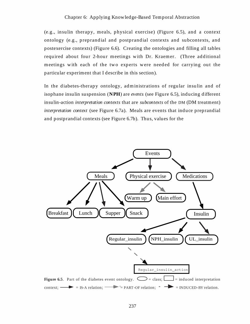
Chapter 6: Applying Knowledge-Based Temporal Abstraction
237
(e.g., insulin therapy, meals, physical exercise) (Figure 6.5), and a context
ontology (e.g., preprandial and postprandial contexts and subcontexts, and
postexercise contexts) (Figure 6.6). Creating the ontologies and filling all tables
required about four 2-hour meetings with Dr. Kraemer. (Three additional
meetings with each of the two experts were needed for carrying out the
particular experiment that I describe in this section).
In the diabetes-therapy ontology, administrations of regular insulin and of
isophane insulin suspension (NPH) are events (see Figure 6.5), inducing different
insulin-action interpretation contexts that are subcontexts of the DM (DM treatment)
interpretation context (see Figure 6.7a). Meals are events that induce preprandial
and postprandial contexts (see Figure 6.7b). Thus, values for the
Regular_insulin NPH_insulin UL_insulin
Breakfast Lunch Supper Snack
Events
Medications
Insulin
Physical exerciseMeals
Warm up Main effort
Regular_insulin_action
Figure 6.5 . Part of the diabetes event ontology. = class; = induced interpretation
context; = IS-A relation; = PART-OF relation; = INDUCED-BY relation.

Chapter 6: Applying Knowledge-Based Temporal Abstraction
238
Glucuse_state_DM_prebreakfast parameter (see Figure 6.4) can be created, when
relevant, regardless of absolute time. The Glucose_state parameter is a new
parameter with six values defined from corresponding ranges used by the
domain expert (HYPOGLYCEMIA, LOW, NORMAL, HIGH, VERY HIGH, EXTREMELY
HIGH). These values are sensitive to the context in which they are generated; for
instance, postprandial values allow for a higher range of the normal value.
Glucose_State value propositions have the value TRUE for the temporal-semantic
property concatenable (see Section 4.2.3) in the same meal-phase context. The
Glucose_State_State parameter is a higher-level abstraction of the Glucose_State
parameter, which maps its six values into three (LOW, NORMAL, HIGH—or L,N,H
for short). It has different semantic properties, and allows creation of daily
horizontal-inference patterns within a nonconvex preprandial context
Contexts
Insulin_action
Regular_insulinaction
DM
Preprandial PostprandialPost_PE
Prebreakfast
Post_PE
Prelunch Presupper
Figure 6.6. Part of the diabetes context ontology. = class; = I S-A relation;
= SUBCONTEXT relation; DM = diabetes mellitus; PE = physical exercise.
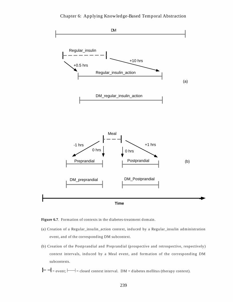
Chapter 6: Applying Knowledge-Based Temporal Abstraction
239
+0.5 hrs+10 hrs
Regular_insulin_action
Regular_insulin
DM_regular_insulin_action
PostprandialPreprandial
+1 hrs
Meal
0 hrs
-1 hrs0 hrs
DM_PostprandialDM_preprandial
DM
Time
(a)
(b)
Figure 6.7. Formation of contexts in the diabetes-treatment domain.
(a) Creation of a Regular_insulin_action context, induced by a Regular_insulin administration
event, and of the corresponding DM subcontext.
(b) Creation of the Postprandial and Preprandial (prospective and retrospective, respectively)
context intervals, induced by a Meal event, and formation of the corresponding DM
subcontexts.
= event; = closed context interval. DM = diabetes mellitus (therapy context).

Chapter 6: Applying Knowledge-Based Temporal Abstraction
240
(see Section 5.1.2) representing abstraction over several meal phases, such as LLH
(LOW, LOW and HIGH Glucose_State_State values over breakfast, lunch, and
supper, respectively).
Patterns such as L L H(Glucose_State_State), especially in the preprandial
subcontext, are extremely useful when a physician must decide how to modify a
patient’s insulin regimen. Furthermore, once created, the prevalence of such
patterns can be calculated—an important step in determining whether the
pattern is a common one for the patient.
Glucose_State_State values that are measured within different phases (e.g.,
prelunch and presupper), but within the same-day, can be joined by
interpolation within the same interpretation context (e.g., a (nonconvex)
PREPRANDIAL context interval, that comprises several preprandial context
intervals), up to 6 to 8 hours apart, the maximal gap being defined by a global ∆
function. In addition, diurnal state abstractions that are measured in the same
phase but over different (usually consecutive) days, such as several values of the
Glucuse_state_DM_prebreakfast parameter, can be joined by interpolation
within the same interpretation context (e.g., a [nonconvex] PREBREAKFAST context
interval, that comprises all breakfasts within a given interval), up 24 to 28 hours
apart.
The temporal-abstraction process is initiated by asserting in an appropriate place
in the temporal fact base an abstraction-goal proposition named DM_PLANNING.
Asserting this proposition initiates the reasoning by inducing a DM
retrospective-context interval for the preceding 2 weeks. This interpretation
context enables, within its scope, creation of the DM domain abstractions. The
time window of 2 weeks is used by the domain expert in practice. It can be easily
modified for particular applications, by changing the declarative definition of the
dynamic induction relation of a context interval (DIRC) (see Section 5.2)
associated with the abstraction-goal proposiiton.
The raw data were originally stored in a text format (patient identification
number, parameter code, time, value). Most of the glucose-parameter codes

Chapter 6: Applying Knowledge-Based Temporal Abstraction
241
referred to specific meal times (e.g., a presupper-glucose code) but some referred
to simply “nonspecific” glucose values, in which case only the time stamp was
known. The data included mostly glucose and insulin codes. Special events
(e.g., physical exercise and larger-than-usual meals) were sometimes reported
too, as well as symptoms of hypoglycemia.
The data were converted into tuples in a relational database. From the database,
it was relatively straightforward to map the data into the RÉSUMÉ temporal fact
base as event and parameter intervals (see Section 5.4), adding the implied
contexts when relevant. From the database, it was also possible to map the data
into a spreadsheet, organizing the data by common measurement times, thus
highlighting contemporaneous events or parameters. The spreadsheet was
useful for the production of graphical charts (Figure 6.8) and spreadsheet tables
(Figure 6.9) during the knowledge-acquisition and evaluation processes.
Patient 30 during 4/1-4/7/91
0
50
100
150
200
250
300
4/1/91
0:00
4/2/91
0:00
4/3/91
0:00
4/4/91
0:00
4/5/91
0:00
4/6/91
0:00
4/7/91
0:00
4/8/91
0:00
Regular
NPH
Nonspec GL
Prebreak GL
Prelunch GL
Presupper GL
Figure 6.8: One of the charts representing data from case 30. Such charts were presented to the
experts as convenient means for detecting temporal patterns. Temporal and statistical
abstractions were marked as intervals on the chart.

Chapter 6: Applying Knowledge-Based Temporal Abstraction
242
I submitted to the two experts (separately) eight data segments from eight
different patients, each segment consisting of 2 consecutive weeks (14 days) of
glucose-measurement and insulin-administration data. The data were presented
to the experts as graphical charts (see Figure 6.8) and as spreadsheets (see Figure
6.9). The spreadsheets were included for additional reference, such as for
Time Regularinsulin
NPHinsulin
Nonspecificglucose
Prebreakfastglucose
Prelunchglucose
Presupperglucose
4/1/91 8:00 5 27 1534/1/91 12:00 3 1374/1/91 22:00 167
4/2/91 8:00 5 27 1624/2/91 12:00 3 1574/2/91 18:00 6 1684/2/91 22:00 197
4/3/91 8:00 5 27 2654/3/91 12:00 3 2434/3/91 18:00 6 2134/3/91 22:00 189
4/4/91 8:00 5 27 1154/4/91 12:00 3 1294/4/91 18:00 6 1644/4/91 22:00 182
4/5/91 8:00 5 27 2124/5/91 12:00 3 1934/5/91 18:00 6 1774/5/91 22:00 201
4/6/91 8:00 5 27 1934/6/91 12:00 3 1764/6/91 18:00 6 1984/6/91 22:00 189
4/7/91 8:00 5 27 2534/7/91 12:00 3 2314/7/91 18:00 6 1814/7/91 22:00 141
Figure 6.9: A portion of a spreadsheet representing data from case 30. Such spreadsheets were
presented to the experts to complement the charts presenting the same data : The spreadsheet
enabled the experts to examine precise values of insulin doses and glucose values.

Chapter 6: Applying Knowledge-Based Temporal Abstraction
243
looking up the precise dose of insulin administered or a glucose value. Overall, I
showed to each expert 112 days of data. Each day included 3 to 4 insulin-
administration events and 3 to 5 time-stamped glucose measurements. Thus,
each expert examined approximately 800 points of data. (The “nonspecific”
glucose measurements such as are shown in Figure 6.9 were mostly bedtime
measurements that were unconnected with a meal, or special measurements,
such as following a hypoglycemia-symptoms episode.)
I asked the experts to mark on the charts the significant point- or interval-based
abstractions (both temporal and statistical) that they would make from the data
for the purpose of therapy. I also asked for their therapy recommendations.
An example of running the RÉSUMÉ system on certain of the data, using as
inputs both the diabetes ontology (Figures 6.4 through 6.6) and the patient-
specific raw data, is shown in Figure 6.10.
In the particular time window shown, two significant findings are demonstrated:
1. A period of 5 days of HIGH presupper blood-glucose values was created by
the abstraction process. This abstraction was returned in response for an
EXISTS_THROUGHOUT external query for a period of at least 3 days of
the Gl_S_S parameter, with value HIGH, in the presupper [nonconvex]
context).
2. A set of three Gl_S_S abstractions representing a repeating diurnal pattern,
consisting of NORMAL or LOW blood-glucose levels during the morning
and lunch measurements, and HIGH glucose levels during the presupper
measurements. Individual abstractions in the set were created by the
abstraction process; the whole set was returned in response to an
OVERALL external set query for Gl_S_S values in the preprandial
[nonconvex] context.

Chapter 6: Applying Knowledge-Based Temporal Abstraction
244
∆
NNH
∆
∆
∆∆∆
Time (date in 1990)
|
Bloodglucosevalues
100
DM_planning_event
DM
200
7/267/257/247/237/22
GLSS_DM_PS
•
•
NNHNLH
•
GLSS_DM_preprandial
H
Figure 6.10: Abstraction of data by RÉSUMÉ in case 3.
= (open) context interval; = abstraction interval; ❒ = prebreakfast glucose; • =
prelunch glucose; ∆ = presupper glucose; DM = diabetes mellitus therapy context; GLSS_DM_PS
= Glucose_state_state abstraction in the DM and presupper context; GLSS_DM_PREPRANDIAL =
Glucose_state_state abstraction in the DM and preprandial context.
The combined pattern suggests that an adjustment of the intermediate-acting
insulin (e.g., NPH) may be indicated. This pattern was noted in the data as
significant by both experts.
Either pattern also can be predefined as an internal PATTERN-type parameter, if
desired. However, the second pattern involves, in the general case, a counting
step (n occurrences of pattern P within a certain period). Counting is a simple
statistical abstraction, but currently outside of the scope of the RÉSUMÉ
temporal-pattern–matching language, which focuses on time and value
constraints. (Statistical patterns could be queried by saving the abstractions in
the database and employing additional temporal-query mechanisms; see
discussion in Section 8.4.2.)

Chapter 6: Applying Knowledge-Based Temporal Abstraction
245
The results of the abstraction experiment are listed in Table 6.2. Together, the
two experts noted 402 abstractions. The abstractions included 218 different
interval-based abstractions (185 temporal abstractions, such as “increasing
glucose values from prebreakfast values to presupper values during the week,”
and 29 different statistical abstractions, such as “large variance of presupper
glucose values”). One hundred and eighty eight different abstractions (164
temporal and 24 statistical) were noted by both experts. Of the remaining 30
abstractions mentioned by only one of the experts, most were noted by only that
expert because the other expert omitted to comment explicitly on the same data
point(s), but his interpretation either was compatible with the first expert’s
abstraction, or clearly supported or implied that interpretation. (Each expert was
asked to comment about other, alternative interpretations, that included the
other expert’s abstractions.) Only nine abstractions overall (six temporal, three
statistical), each of which was created by just one of the experts, were indeed
noncompatible abstractions of the same data (that is, mutually exclusive with the
bstractions created for that time period by the other expert). For example, in one
abstraction, one expert interpreted a particular pattern of early morning
hypoglycemia followed by a high prebreakfast glucose value as a possible
Table 6.2: Abstractions formed by two experts in the diabetes domain.
Expert Temporal abstractions Statistical abstractions Total
compatible noncompatible compatible noncompatible
I 179 2 24 1 206
II 164 4 26 2 196
subtotal 343 6 50 3 402
Total 349 53 402

Chapter 6: Applying Knowledge-Based Temporal Abstraction
246
a Somogii effect.13 The other expert interpreted the same sequence as rebound
hyperglycemia caused by increased food intake due to the hypoglycemia
symptoms. Other idiosyncratic abstractions included noting a pattern of very
high glucose levels following larger than usual meals during particular phases of
the day, a pattern of low prebreakfast and high presupper glucose values in the
context of an UltraLente insulin regimen, a high variance in bedtime glucose
measurements, and a weekend “large brunch” phenomenon.
Since all the 164 compatible abstractions mentioned by Expert II were mentioned
by Expert I, I considered that set as the set of common abstractions. The
RÉSUMÉ system created 132 (80.4%) of the 164 temporal abstractions noted by
both experts. None of the nine noncompatible abstractions mentioned by only
one of the experts were created; these abstractions usually involved complex
temporal or statistical contexts, such as contexts defined by particular insulin
regimens or by glucose variance and minima during specific diurnal phases.
Additional characteristics of the abstractions that proved hard to create are
discussed in Section 6.4.
As was the case in the domain of monitoring children’s growth, the RÉSUMÉ
system produced many additional abstractions, most of which were low- and
intermediate-level abstractions such as glucose-value range classifications and
gradient abstractions, and intermediate-length abstractions. Again, most of these
could be viewed as partial computations that are invisible to a user that defines a
particular internal pattern or that asks a particular external query, but that are
useful for anticipating potential queries. For reasons of limited expert time, not
all these low-level abstractions were examined. Examination of the output for
the first three cases with one of the experts showed that the expert agreed with
almost all (97%) of the produced abstractions, a similar result to the one
presented in the domain of growth monitoring. This high predictive value was
expected, since the domain ontology directly reflected that expert’s knowledge
13 A Somogii effect occurs when an excess of insulin lowers the blood glucose to a state ofhypoglycemia, thus invoking several hormonal defense mechanisms that increase the bloodglucose. The overall effect is a paradoxical (rebound) elevation of the blood glucose in thecontext of a sufficient and even too large insulin dosage.

Chapter 6: Applying Knowledge-Based Temporal Abstraction
247
about these low- and intermediate-level abstractions. In the few cases with
which the expert did not agree, the reason was often due to the rigid
classification of ranges (e.g., a blood-glucose value of 69 mg/dl glucose should
not have been interpreted as LOW even if the expert agreed that, in general,
normal values lie between 70 mg/dl and 110 mg/dl). I discuss the range-
classification issue in Section 8.4.
Of considerable interest (and quite different from the result we expected) is the
fact that, although the abstractions identified by the two domain experts were
remarkably similar, the therapy recommendations suggested by the experts differed
for all of the eight cases (Table 6.3). I discuss the meaning of this result in Section
6.4.
Another surprising result was that both experts arrived at most of their
conclusions by looking only at the graphical charts produced from the
spreadsheets (see Figure 6.8), whose data representation was rather qualitative
and more suitable for general temporal-pattern matching. The detailed
spreadsheets (see Figure 6.9) were used almost exclusively only when the therapy
options were considered (e.g., increasing the regular-insulin dose in the morning
required looking at the current dose of that and other insulin types). The
phenomenon would seem to suggest that the experts base most of their
conclusions on context-sensitive patterns of blood-glucose value (e.g., HIGH
fasting [prebreakfast] glucose values in a patient that is being treated by a
regimen of NPH and regular insulin twice a day), and need the actual doses of
insulin only infrequently.

Chapter 6: Applying Knowledge-Based Temporal Abstraction
248
Table 6.3: Therapy recommendations made by the diabetes experts
Case
ID
Current insulin-therapy
regimena
Expert I
recommendation
Expert II
recommendation
1 NPH at MT
REGx3 (MT, LT, DT)
Check lifestyle
(highly erratic)
Add NPH at BT
2 REGx4 (MT, LT, DT, BT) Add NPH at BT Add NPH at BT
Increase REG at MT
3 UL at MT, DT
REG at AM, DT
Substitute UL at MT
by NPH at MT, DT
Add REG at LT
5 NPH at MT, DT
REG at AM, DT
Increase NPH at MT,
decrease NPH at DT
Increase NPH at MT,
then adjust REG, ifnecessary
6 NPH at MT
REGx3 (MT, LT, DT)
Decrease dinner meal
or add NPH at BT
Shift NPH to BT,
then add NPH at MT,if necessary
7 NPH at MT
REGx3 (MT, LT, DT)
Check life style,
change diet
Check life style,
change diet,
reduce REG whenglucose is low
30 NPH at MT
REGx3 (MT, LT, DT)
Substitute NPH at MTby UL at AM
or shift NPH to BT andincrease REG beforemeals
Shift NPH to BT
55 UL at MT
REGx4 (MT, LT, DT, BT)
Substitute UL at MT
by NPH at BT,
remove REG at DT
Increase UL at MT,
shift REG at MT to LT
remove REG at DT
aMT = morning time; LT = lunch time; DT = dinner time; BT = bedtime; REG = regular insulin;NPH = isophane insulin suspension; UL = UltraLente.

Chapter 6: Applying Knowledge-Based Temporal Abstraction
249
6.4 Discussion and Summary
In previous chapters, I have presented mainly the theoretical and the potential
merits of the knowledge-based temporal abstraction method. In this chapter, I
have evaluated the implementation of that method as the RÉSUMÉ system. By
doing so, I have added an empirical weight to my argument. I have argued that
most of the desired properties that were emphasized by previous researchers in
clinical summarization systems (see Section 3.2), and, in particular, all of the
requirements for temporal-abstraction systems which were listed in Section 1.1,
are either inherent in the representational and computational aspects of the
knowledge-based temporal-abstraction method or are an integral part of the
RÉSUMÉ architecture. I will discuss this claim in detail in Section 8.2.
In this chapter, I have presented initial, encouraging results regarding
representation of several different temporal-abstraction tasks in several different
clinical domains using the knowledge-based temporal abstraction methodology.
I also have demonstrated positive results of applying certain of the resulting,
domain-specific temporal-abstraction systems to a number of clinical test cases,
some of which (those involving growth monitoring and diabetes therapy)
originated in domains that differ significantly from the one that supplied the
original motivation for developing a domain-independent, task-specific
architecture for temporal abstraction.
Each clinical application domain demonstrated different facets of the RÉSUMÉ
system. Due to their diversity, none of the domains truly tested all of the aspects
of the RÉSUMÉ system and the underlying knowledge-based temporal-
abstraction methodology.
The “tall” ABSTRACTED-INTO ontology of the growth-monitoring domain
challenged mainly the capabilities of the contemporaneous-abstraction and
temporal-pattern–matching mechanisms to perform multiple-parameter
abstraction, given any level of abstraction in the input (e.g., accept not only raw

Chapter 6: Applying Knowledge-Based Temporal Abstraction
250
height measurements and Tanner maturation stages as input, but also the
intermediate-level parameters HTSDS and Maturation). The number of input
data points per case was rather small, as is typical for this sparse-data domain.
The protocol-based–care domains did include many data points, and the breadth
of the parameter ontology was considerable (clinical protocols often involve
many dozens of primitive parameters). However, the depth of the ontologies of
those domains was not due to the ABSTRACTED-INTO relation, but rather was due
to the specialization of the abstractions, by the IS-A relation, into different
contexts. These contexts, some direct and some prospective, were induced
mainly by different phases of therapy or by different medications, demonstrating
the use of the context-forming mechanism and of the event and context
ontologies. In addition, the hematological abstractions over weeks and months
required the use of dynamic temporal knowledge (i.e., local and global
persistence knowledge) by the temporal-interpolation mechanism. Finally, due
to laboratory data coming out of temporal order, or modifications in existent
laboratory-data values, these domains demonstrate the importance of
maintaining logical dependencies by the truth-maintenance system.
The diabetes therapy domain included only one laboratory parameter (glucose
values at different phases of the day) and one qualitative parameter
(hypoglycemia symptoms) and several events (different types of insulin
administrations, meals, and physical exercise). However, the emphasis on
temporal and statistical dimensions in that domain made abstracting concepts
that are meaningful for therapy purposes quite challenging, and pushed the
temporal-inference and temporal-pattern matching mechanisms to their limits.
In fact, the results of the relatively small experiment have shown that additional
features are needed for a complete temporal-abstraction architecture that is
suitable for supporting the treatment of insulin-dependent patients. (Most of the
required features are in fact planned for a future system that will include in its
architecture the RÉSUMÉ system discussed in this dissertation.)

Chapter 6: Applying Knowledge-Based Temporal Abstraction
251
I have noticed three limitations of the current RÉSUMÉ system with respect
to the challenging diabetes-therapy domain:
1. There are difficulties in querying general cyclical (e.g., diurnal) patterns,
especially patterns dependent on external times. In the current design
of the diabetes knowledge base, for instance, diurnal patterns are
detected through horizontal-inference tables (e.g., creating an LLH
abstraction for prebreakfast, prelunch and presupper times). It would
have been awkward to represent, say, a repeating pattern of LOW
bedtime glucose followed by HIGH prebreakfast glucose. First, the
“bedtime” abstraction would have to be created as a repeating, cyclic
abstraction—say, the absolute , external , time being about 10 p.m. each
day. But absolute time is currently converted in RÉSUMÉ to the more
common internal time (e.g., patient-age in the growth-monitoring
domain; days of therapy in the protocol-based care domains), and only
one time stamp is kept. Similarly, a “weekend” abstraction would be
awkward to define. Representing both external time (e.g., 10 p.m.) and
internal time (e.g., 5 days of therapy) might enable RÉSUMÉ to create
both types of temporal abstractions. Second, bridging the gap between
bedtime and prebreakfast time would be prevented by the preprandial
interphase ∆ functions that currently permit bridging only shorter gaps
(e.g., from lunch to dinner), thus keeping the abstractions within the
same day. The join might need to be defined as a temporal-pattern, or
as an extension of ∆ functions that enables different contexts.
2. There is a difficulty in integrating statistical queries (e.g., means and
standard deviations) with temporal queries. The statistical queries are
straightforward (mean, variance, minimum, maximum, general
distribution, count) and usually can be queried through the underlying
database. However, the statistical computation needs a temporal context
(e.g., prelunch times) in which to operate, and a temporal scope to limit

Chapter 6: Applying Knowledge-Based Temporal Abstraction
252
the computation (e.g., previous 2 weeks). I discuss a possible solution
in Section 8.4.2.
3. It might have been desirable to detect patterns defined by events, such as
insulin use, in addition to those defined by parameters , such as glucose
states. Such a requirement has not been noted in other domains, since the
external events were usually assumed to be controlled by the human or
automated therapy planner (e.g., chemotherapy administration was
controlled by the physician and the current protocol was well known). Such
event-based patterns in the diabetes domain might generate more
meaningful interpretation contexts, by detecting periods in which the
patient varied her own therapy significantly, or by detecting insulin-therapy
regimens implicit in the data but never asserted by the physician or the
patient (see Table 6.3 for examples of insulin-therapy regimens). Such early
work in the diabetes domain has been described by Kahn and his colleagues
[Kahn et al., 1990], with encouraging results. Alternatively, complex
contexts might be asserted in the temporal fact base by the user before the
RÉSUMÉ system is called for performance of abstraction.
These insights seem more significant than the measures of sensitivity and
predictive value I have presented in the domains of monitoring growth and
treatment of diabetes. The number of generated abstractions or their accuracy is
useful for some purposes but might be highly misleading with respect to
evaluating a temporal-abstraction system. As I have mentioned, many of the
abstractions that RÉSUMÉ generates can be viewed as partial computations.
These partial computations are cached, and have an important role for truth
maintenance purposes and for answering multiple-level queries. Most of these
abstractions are invisible to the user, whether a human or an automated therapy
planner, and are used by the temporal-pattern–matching mechanism for
detecting internal (predefined) or external (online) temporal patterns. Therefore,
the question I have attempted to answer usually was “would the system be able to
answer the temporal queries that the user needs for performance of the task at hand?” In

Chapter 6: Applying Knowledge-Based Temporal Abstraction
253
this respect the results were quite encouraging, although, as I have listed above,
there is some room for extensions.
Although the abstractions identified by the two domain experts were remarkably
similar—there were few differences in the interpretation of the various data
segments presented—the therapy recommendations suggested by the experts
differed for all of the eight cases (see Table 6.2). This observation would seem to
validate one of the basic premises underlying the goal of the temporal-
abstraction task—namely, that intermediate conclusions from the data (the
interval-based abstract concepts and patterns) are significantly more stable than
are specific therapy rules predicated on these conclusions. Thus, knowledge
about forming the intermediate patterns should be represented explicitly and
separately from knowledge about therapy, which might depend on the expert’s
level of comfort and experience with particular forms of therapy when several
legitimate options exist, as is the case for insulin-dependent DM. The optimal
therapy might also depend on the patient’s preferences (e.g., using a long-acting
insulin and thus reducing the number of injections per day might be considered
desirable by the patient, even though control of glucose is not optimal). In other
words, therapy also implies a physician model and a patient model of utilities of
various options, and should not be confused with the interpretation task.
The observation that both experts in the diabetes domain seemed to rely almost
exclusively on the rather qualitative graphical charts for interpretation of the
data, and used the full spreadsheets only for final decisions on therapy
modification, is significant. This observation lends further support to the use of
the qualitative interpretation contexts as a major tool for organizing temporal-
abstraction knowledge. For instance, both experts noted immediately, before
creating a single abstraction, particular temporal patterns of insulin
administration (e.g., one NPH-insulin shot in the morning and three regular-
insulin shots during morning, lunch and supper). It did not seem to matter what
were the precise doses involved. This behavior is analogous to the way the
context-forming mechanisms creates context intervals: Events and abstractions
induce interpretation contexts that are mostly qualitative, such as “regular-

Chapter 6: Applying Knowledge-Based Temporal Abstraction
254
insulin action” or “therapy by high-dose AZT.” Within these context intervals,
creation of abstractions is highly focused.
My initial assessment of the knowledge-acquisition requirements for typical clinical
domains is based on the experience I gained in applying the knowledge-based
temporal-abstraction method to the AIDS protocol-based–care domain, to the
chronic GVHD domain, to the growth-chart–monitoring domain, and to the
diabetes-therapy domain. My experience in these application areas suggests
that, for any particular context in one of these domains, a significant, but
manageable amount of knowledge must be acquired. This knowledge must be
entered either by the knowledge engineer who designs the system, or by a
clinical expert from whom specific knowledge (e.g., classification tables) is
acquired and represented in the domain’s temporal-abstraction ontology. Both
these users can benefit from an automatically generated knowledge-acquisition
tool that can acquire the appropriate domain-specific knowledge needed to
instantiate the temporal-abstraction mechanisms (see Chapter 7).
The minimal amount of clinical knowledge that needs to be acquired includes (1)
the primitive or abstract clinical parameters relevant to the task and their
structural relations—in particular, IS-A and ABSTRACTED-INTO relations
(including all the relevant abstractions of these parameters, classified into the
four basic abstraction types: state, gradient, rate, and pattern); (2) a clinically
significant change for each relevant primitive parameter, if gradient abstractions
are required; (3) the list of potential state- and rate-abstraction values for all
parameters relevant to the task for which these abstraction types are required;
and (4) the maximal-gap ∆ functions, when interpolation is required in the task,
for each relevant parameter and context.
The inferential (temporal-semantic) properties, gradient-abstraction horizontal-
inference values, and the interpolation-inference tables are more stable than the
knowledge types listed above, and are less dependent on the interpretation
context. The default values for these types of temporal-abstraction knowledge
either can be inherited through the appropriate abstraction class (e.g., state

Chapter 6: Applying Knowledge-Based Temporal Abstraction
255
abstractions), or can be acquired for only the most general parameter class (e.g.,
platelet state abstractions in the context of the overall task). As additional
applications are designed, the gain in development time is more apparent, as I
have noticed in the case of the several subdomains of protocol-based care.
Although instantiating the temporal-abstraction mechanism for a new domain
would appear superficially to involve significant amounts of knowledge
acquisition, it is, in fact, important to note the following encouraging results of
my experiments with respect to this aspect of the methodology:
1. The major knowledge-acquisition effort in these nontrivial domains
usually required two to four meetings (each 1 to 2 hours long) with the
expert—a tenable amount of time. Also, the size of the ontologies was
certainly manageable, even though one or more explicit, intermediate
levels of abstraction were added. The addition, however, was related to
the abstraction levels of the expected input and of the expected queries.
Furthermore, maintenance of the resultant knowledge base by the
knowledge engineer, including additional classifications by the expert,
required significantly less time than would be needed to create or modify
pure programming code.
2. The knowledge-acquisition process was driven by the knowledge-based
temporal-abstraction method, thus creating a purposeful structure to the
process, and enabling the knowledge engineer to predict, for instance, a
possible existence of a gradient abstraction of a state abstraction of a
known parameter. Thus, a certain measure of completeness is
guaranteed. Additional sessions served to explore and refine the
evolving parameter, event, and context ontologies, as was particularly
apparent in the growth-monitoring domain [Kuilboer et al., 1993]. Dr.
Kuilboer and I felt that, without that methodology, it is doubtful whether
either of us would progress very far in a few meetings with the expert, or
whether I would be able to share and reuse the knowledge acquired by
Dr. Kuilboer.

Chapter 6: Applying Knowledge-Based Temporal Abstraction
256
3. Most important parameters and their values must be represented in one
way or another to perform the temporal-abstraction task at hand.
Hematological toxicity tables (in protocols for treatment of AIDS or
chronic GVHD), HTSDS rate abstractions (in the growth-monitoring
domain), and ranges and patterns of blood glucose in the domain of caring
for diabetes patients need be noted in some fashion. Thus, most of the
knowledge-acquisition effort was really spent on organizing in a useful
architecture a significant amount of knowledge that must be accessed and
represented, implicitly or explicitly, to solve the task. Explicit
representation, as I have shown, has multiple additional benefits; in the
experiments that I have conducted, its cost was not too prohibitive, while
the results seemed to justify the effort.

Chapter 7: Acquisition of Temporal-Abstraction Knowledge
257
7 Acquisition of Temporal-AbstractionKnowledge
In Chapter 4, I defined the knowledge-based temporal-abstraction method, an
inference structure that solves the temporal-abstraction task by decomposing that
task into five subtasks (see Figure 1.2). Each subtask can be solved by one of five
separate temporal-abstraction mechanisms (see Section 4.2). I defined four
domain-specific knowledge types (structural, classification, temporal-semantic, and
temporal-dynamic) that are used as knowledge roles (see Section 2.1) by the
temporal-abstraction mechanisms. The four knowledge types and their precise
use by the mechanisms were described formally in Chapter 4. The subtypes of
the four main categories of domain-specific knowledge were described in Section
5.1. The representation of every subtype of domain knowledge in the RÉSUMÉ
system was discussed in Sections 5.1 through 5.4.
In Chapters 2 through 5, I elaborated the various advantages of explicit
representation of the knowledge needed for abstracting data over time, such as
enabling the reuse of domain-independent, but task-specific, temporal-abstraction
mechanisms, and the sharing of some of the domain-specific knowledge by
different problem solvers. In particular, I explained in Chapter 2 the rational for
a knowledge-level analysis and representation of problem-solving methods. One
of my goals in categorizing the various types and subtypes of the domain-specific
knowledge needed for abstraction of time-stamped data, and for designing the
frame-based parameter-properties ontology, was to facilitate the acquisition of
that knowledge from several possible sources. Once we understand the
knowledge required for temporal abstraction (e.g., temporal inferential
properties), and have constructed a model of the use of that knowledge, it is
easier to acquire the particular knowledge that can play the role we need in the
knowledge-based temporal-abstraction method. It is also easier to maintain the

Chapter 7: Acquisition of Temporal-Abstraction Knowledge
258
acquired knowledge when the role of every piece of knowledge is well defined
[McDermott, 1988].
There are three possible approaches to the task of acquiring the knowledge
required by the temporal-abstraction mechanisms. All approaches exploit the
formal, explicit representation of the temporal-abstraction knowledge types. In
Sections 7.1 through 7.3, I elaborate these approaches. The three approaches are
not mutually exclusive, and might even complement each other.
7.1 Manual Acquisition of Temporal-Abstraction Knowledge
One possibility for acquiring temporal-abstraction knowledge is to use classical
manual or semimanual knowledge-acquisition (KA) techniques that have been
developed to elicit knowledge by direct interaction of the system developer with
domain experts. Such techniques include, for example, analysis of verbal
protocols documenting the expert’s problem-solving process (e.g., [Ericsson and
Simon, 1984]), or construction of repertory grids that associate domain
constructs (e.g., findings such as “low blood pressure”) with domain elements
(e.g., diagnoses such as “myocardial infarction”). Tools have been built that
facilitate construction of repertory grids [Boose and Bradshow, 1986]. However,
these particular approaches conceal the actual problem-solving method implied by
the KA tool.
The knowledge roles defined by the knowledge-based temporal-abstraction
method and by the mechanisms that I suggest for performing the subtasks that
that method posts are explicit. The explicit roles suggests using at least a
method-specific KA approach [Musen, 1989b]; that is, acquisition of precisely the
knowledge required by the five temporal-abstraction mechanisms (e.g.,
temporal-semantic knowledge). Furthermore, for any particular domain, a task-
specific approach [Musen, 1989b] is indicated; that is, we can acquire precisely
the knowledge required for instantiating the temporal-abstraction mechanisms
for a particular task in a particular domain (e.g., only knowledge required for
creating state and gradient abstractions, but not for creating rate abstractions,
and for only a particular class of parameters). Task-specific KA tools require that

Chapter 7: Acquisition of Temporal-Abstraction Knowledge
259
we use the terms of the domain, such as cycles of chemotherapy. Note that the
original PROTÉGE system [Musen, 1989a] was a method-specific KA tool, which
generated task-specific KA tools similar to OPAL [Musen et al., 1987] (see Section
2.2). Both were automated tools.
However, method- and task-specific KA techniques do not have to rely on
automated tools, such as OPAL; they also can be manual. Note that use of the
term manual here does not mean that the knowledge is acquired in some ad hoc
manner. On the contrary, if the knowledge engineer knows what knowledge she
requires, and manages to build a good conceptual model of the problem-solving
method that underlies the system being designed, she can elicit that knowledge
and incorporate it into the conceptual model of the task that she is constructing.
Incorporating the knowledge will be done in a principled manner, such that the
use of the knowledge will be well defined, and its maintenance facilitated. The
emphasis in that case is on a principled approach driven by a well-defined
model.
I have used manual techniques for acquiring the knowledge required by the
knowledge-based temporal-abstraction method in the domains of protocol-based
care, pediatric growth monitoring, and therapy of insulin-dependent diabetes. In
the protocol-based–care domain (see Section 6.1), apart from using written
protocols (CCTG-522 and PAZ), I interviewed a domain expert (J. Sisson, M.D.)
and acquired the knowledge needed for instantiating the RÉSUMÉ problem
solver in the case of a protocol for prevention of toxoplasmosis infections in
patients who have HIV infection. In the domain of pediatric growth monitoring,
Dr. Kuilboer acquired, with my assistance, the growth-chart–analysis parameter-
properties ontology that was described in Section 6.2 (see also Figure 6.2). In the
domain of treatment of patients who have insulin-dependent diabetes, I acquired
the knowledge from one of the two domain experts who participated in the
experiment (see Section 6.3).
In all three domains, I found the RÉSUMÉ methodology highly useful. The
methodology implied by the knowledge-based temporal-abstraction method

Chapter 7: Acquisition of Temporal-Abstraction Knowledge
260
focused the KA effort on the essential input and output parameters and their
structural relations, on the potential abstractions of these parameters, and on the
four types of knowledge necessary to create the desired output abstractions in
each domain. The advantages were especially obvious when another knowledge
engineer (Dr. Kuilboer), who was not familiar with the internals of the RÉSUMÉ
system, acquired a complete temporal-abstraction ontology from an expert in the
domain of monitoring children’s growth (see Section 6.2). In that case, the only
support for Dr. Kuilboer was the knowledge-based temporal-abstraction model
and the declarative description of the knowledge she was eliciting. Since
maintenance of the evolving ontology by both Dr. Kuilboer and, eventually, by
myself was part of the KA process, it was doubly important to clarify what was
the role of the knowledge acquired in each refinement cycle [Kuilboer et al.,
1993].
One conclusion I can draw from these experiments is that, in domains such as
monitoring growth and therapy of insulin-dependent diabetes, which have a
small number of primitive parameters but many levels of abstraction from these
parameters or many context-specific specializations, the primary KA task is to
acquire the structural domain knowledge. This knowledge type is embodied in
the parameter, event, and context ontologies as various qualitative relations (e.g.,
IS-A, PART-OF, ABSTRACTED-INTO, SUBCONTEXT relations) and, once acquired,
limits the scope of the rest of the KA process to acquiring knowledge about
relevant parameters and contexts. Thus, the structural knowledge drives the
process of KA for the parameter-properties ontology (e.g., the arguments of the
classification functions or tables should be known by the time the entries are
acquired). It was reasonably straightforward, once the structural knowledge was
acquired, to refine the parameter-properties ontology, the event ontology, and
the implied interpretation-contexts ontology by filling (or inheriting from higher
abstraction classes) classification, inference and interpolation tables.
In addition, it was both necessary and helpful to motivate the cooperation of the
experts in this process by explaining the knowledge roles that these tables play in
the problem-solving process. The problem-solving method used by the RÉSUMÉ

Chapter 7: Acquisition of Temporal-Abstraction Knowledge
261
system is not intuitive. Nevertheless, the steps that all experts took in their
eventual analysis of the data were remarkably similar, on close inspection, to the
inference structure of the RÉSUMÉ system's underlying knowledge-based
temporal-abstraction method. Thus, it was useful to point out the similarities.
As I mentioned in Section 6.4, the minimal amount of clinical knowledge that I
needed to acquire in the three domains included (1) the parameters (and all
abstractions of these parameters) relevant to the task and their structural
relations—in particular, IS-A and ABSTRACTED-INTO relations; (2) a clinically
significant change for each relevant primitive parameter, if gradient abstractions
were required; (3) the list of potential state- and rate-abstraction values for all
parameters relevant to the task for which these abstraction types were required;
and (4) the maximal-gap ∆ functions, when interpolation was required in the
task, for each relevant parameter and context. Inferential (temporal-semantic)
properties, gradient-abstraction horizontal-classification tables, and the
qualitative interpolation constraints inherent in the interpolation-inference tables
were usually more stable than the knowledge types listed above, and were less
dependent on the interpretation context. The default values for these knowledge
categories either could be inherited through the appropriate abstraction class
(e.g., state abstractions), or could be acquired for only the most general
parameter class (e.g., platelet state abstractions in the context of the overall task).
Thus, manual method-specific and task-specific KA techniques can certainly
exploit well-defined problem-solving principles, and can use the latter to build a
conceptual model of the task, such that the knowledge acquired from the expert
will play predefined roles. In particular, manual techniques can take advantage
of the four formal knowledge types defined by the knowledge roles of the five
temporal-abstraction mechanisms.
7.2 Automated Acquisition of Temporal-Abstraction Knowledge
The second option for acquiring temporal-abstraction knowledge is to use
automated KA tools, such as those produced by the PROTÉGÉ-II project [Puerta
et al., 1992; Musen, 1995] (see Section 2.2). In this way, we exploit the power of

Chapter 7: Acquisition of Temporal-Abstraction Knowledge
262
method-specific and task-specific KA tools, and combine that power with the
advantage of generating an automated tool that can interact with the domain
expert without intervention of the knowledge engineer, assuming that the proper
ontological commitments (e.g., defining an event ontology for the domain) have
been specified at the level of the PROTÉGÉ-II user.
One issue that developers must consider when designing automated KA tools is
the ontology-mapping process. Problem-solving methods have their own
private model of the data on which they operate, a method ontology, that should
be mapped onto the description of the particular domain modeled by the
knowledge-based system, the domain ontology. Ontology mapping should be
sufficiently general to include complex structures, relations, and inference
methods. The process of mapping ontologies includes an instantiation of the
knowledge roles of the problem-solving method by particular domain structures,
or by transformation functions of domain structures (e.g., drug-toxicity tables in
the domain of protocol-based care can be mapped into the vertical-classification
knowledge role of the knowledge-based temporal-abstraction method). The
PROTÉGÉ-II group has been working on defining classes of such mappings
[Gennari et al., in press]. However, certain knowledge roles in the problem-
solving method might not be filled at all by direct mapping, since the domain
may not normally contain any structures that can easily be mapped to these roles
(e.g., maximal-gap ∆ functions or local-persistence ρ functions). Thus, the
domain’s basic, core ontology (devoid of any task-specific aspects) might have to
be augmented by the terms of the particular method using it. I term that the
ontology-enhancement process. These method-specific terms might be useful to
other methods (e.g., propositional inference types, such as the concatenable
inferential property, might be useful for other problem-solvers and other tasks)
and might even be shared with these methods; but they (or their equivalents) do
not exist in the domain’s core ontology. Whether, in general, application
domains have any such platonic core ontologies is perhaps a philosophical issue,
but it assumes crucial importance when a method’s ontology has to be
instantiated by domain terms. In any case, to develop a KA tool for the

Chapter 7: Acquisition of Temporal-Abstraction Knowledge
263
knowledge-based temporal-abstraction method will involve augmenting the
domain of interpretation by terms that denote knowledge types that do exist
implicitly in the domain, as my knowledge-acquisition experiments show, but in
no obvious, easy to identify form.
Another important issue that a designer of a knowledge-based system must
consider when developing a KA tool for a method such as the knowledge-based
temporal-abstraction method is whether a stable domain ontology exists when
the KA process takes place; I term this issue the fluid-ontology problem. Tools
of the OPAL type, and even of the PROTÉGÉ type [Musen, 1989a], assume a
stable domain ontology, usually defined by the knowledge engineer. The
domain ontology, once defined, drives the task-specific KA process. For
instance, the ESPR method discussed in Section 2.2, as represented in PROTÉGÉ,
assumed the existence of well-defined planning entities [Musen, 1989a]. The
planning entities can be combined to form plans; the names and attributes of
these entities can be used as domain-specific labels in a task-specific graphic
interface of a tool such as OPAL. In other words, the OPAL and PROTÉGÉ
models assumed that the structural knowledge is relatively straightforward to
represent, and can be modeled even by the designer of a new system (e.g., major
entities in the domain, such as chemotherapy and radiotherapy events, and their
interrelationships) and that, based on the stable top-level ontology, a KA tool can
be generated that uses the domain terms. This, in fact, is often the case when
applying the ESPR method to the task of supporting treatment with clinical
guidelines in a particular domain.
However, in the case of the knowledge-based temporal-abstraction method, the
knowledge inherent in the ontology entities and relations themselves is often a
crucial and major part of the knowledge needed by the temporal-abstraction
mechanisms—namely, the structural knowledge types and subtypes. The
structural knowledge is important for the event ontology, for the context
ontology, and for the parameter-properties ontology. Therefore, a prerequisite to
efficient acquisition of parameter-properties ontologies is the ability to acquire
and modify easily domain ontologies at KA time, as part of the KA process (i.e.,

Chapter 7: Acquisition of Temporal-Abstraction Knowledge
264
while interacting with the domain expert), not just at the time of designing a
specific KA tool. The PROTÉGÉ-II group is, in fact, developing ontology
modeling tools, such as Maítre [Gennari, 1993]. These tools are intended mainly
for knowledge engineers, and are highly useful for modeling and for maintaining
ontologies of new domains by a developer. In general, however, the knowledge
engineer cannot define alone the domain’s complete ontology, or even a
significant part of it. Most of the KA process might comprise acquiring the
domain’s structure, including the definition of intermediate levels of abstraction,
as was the case when acquiring the growth-monitoring ontology (see Section 6.2).
This implies that the ontology-modeling tool might be, in the case of problem-
solving methods such as the knowledge-based temporal-abstraction method and
its mechanisms, the major method-specific KA tool for the domain expert, since
acquiring the domain’s basic ontology might be the main KA process we are
trying to automate.
The third issue brought up by the possibility of automated acquisition of
temporal-abstraction knowledge, and especially by the prospect of acquiring a
temporal-abstraction ontology, is how to enforce semantic relations, between
different parts of the ontology, during the KA process. I term this the semantic-
enforcement problem. For instance, as explained in Section 4.2.1, events and
event chains, among other propositions, can induce (directly or indirectly) basic
and composite interpretation contexts, respectively. (Abstraction goals and
context-forming parameter propositions also can induce, of course, interpretation
contexts, as defined by the set of DIRCs.) Thus, splitting nodes in the IS-A
hierarchy of the parameter ontology (see Figure 5.2), by distinguishing between
at least two different subcontexts of the current node’s interpretation context for
the same parameter, is an operation that must chose between at least two
legitimate interpretation contexts. These interpretation contexts must be defined
at some point somewhere in the domain’s temporal-abstraction ontology; the
definition might involve adding one or more relations such as DIRCs, SUBPART
relations and SUBCONTEXT relations.

Chapter 7: Acquisition of Temporal-Abstraction Knowledge
265
For instance, Hb_State_CCTG might be the node representing knowledge about
the state abstraction of Hb within the interpretation context induced by the
CCTG protocol (see Figure 5.2); splitting that node (creating two or more
descendant nodes) might involve distinguishing between at least two
interpretation contexts. These more specialized, composite , interpretation contexts
could be, for instance, induced by events that have a PART-OF relation, in the
event ontology, to the CCTG protocol (e.g., the AZT and the T/S regimens; see
Figure 5.3), and thus might induce interpretation contexts that have a
SUBCONTEXT relation to the interpretation context induced by the CCTG event.
Other options for creating a legitimate composite interpretation context include
the use of any other interpretation contexts that have a SUBCONTEXT relation, in
the context ontology, to the interpretation context induced by the CCTG protocol.
Such interpretation contexts might be induced, for instance, by context-forming
parameter propositions that exist in other parts of the parameter ontology (e.g.,
the SEVER-LEUKOPENIA value of the WBC_State parameter in the context of the
CCTG protocol).
Thus, when the user tries to split a node in the parameter-properties ontology,
the KA tool should be able to judge that a new interpretation context is needed,
to check in either the parameter ontology, the event ontology, or the context
ontology if the new context created is a legitimate one, to suggest choosing or to
assist in constructing a default legitimate interpretation context, and, when
necessary, to augment the context ontology of the domain by a new
interpretation context, that has been defined during the KA process. Provision of
such a semantic-enforcement feature requires sophisticated tools. In effect, the
ontology of the domain should be built by a recursive, bootstrapping process.
However, that process clearly resembles the iterative manual process that I
experienced in several domains, in particular in the domain of monitoring
children’s growth [Kuilboer et al., 1993]. Thus, there is a need for investigating
the automated-KA needs of complex methods, such as the knowledge-based
temporal-abstraction method, in the context of the PROTÉGÉ-II project.

Chapter 7: Acquisition of Temporal-Abstraction Knowledge
266
7.3 Knowledge Acquisition Using Machine Learning
The third option for acquisition of some of the knowledge required for
instantiation of the temporal-abstraction mechanisms is to use different
techniques to acquire the qualitative and the quantitative aspects of the temporal-
abstraction knowledge.
It should be straightforward to acquire the qualitative knowledge types that
domain experts find intuitive, such as inferential properties and classification
tables, manually or through an automated KA tool. However, we might learn
some of the quantitative knowledge, such as local-persistence (ρ) and maximal-
gap (∆) functions, using machine learning (ML) techniques, by inspecting large,
time-oriented clinical databases. In Section 4.2.4.1 I elaborated on a probabilistic
interpretation of persistence functions, and I showed that, under certain
conditions, maximal-gap ∆ functions might be much simpler to express and to
acquire than the implicit forward- and backward-belief–decay ρ functions that
generate these functions. Thus, if we assume that the data are consistent, and
that there is some simple polynomial function describing the persistence of those
data, then it might be possible, given sufficient time-stamped data, to learn that
polynomial function, using an ML approach.
To do that, we might ignore systematically certain parameter points, forming
artificial gaps in the input data, and ultimately check the value of the primitive or
abstract parameter during the gap.
At the very least, we should be able to form upper and lower bounds on
particular ∆(π, L(I1), L(I2)) values—namely, on the maximal-gap persistence of a
parameter when it was true over one time interval before the temporal gap and
true over another time interval after that gap.
For instance, if we express ∆ just as a function of the lengths of the two intervals,
L(I1), L(I2)—or L1 and L2 for short—and if we are trying to fit the data with a
linear maximal-gap function ∆ such that

Chapter 7: Acquisition of Temporal-Abstraction Knowledge
267
∆(L1, L2) = AL1 + BL2 + C
then a good starting point would be looking for the maximal time gap between
two consecutive parameter points such that π does not change its value inside the
gap. Thus, we can get an estimate of C when L1 = L2 = 0:
∆(0, 0) = C,
for joining point parameters.
If we assume that the function is a PP ∆ function (see Section 4.2.4.1.3), then the
possibilities are constrained further, since
∀ (L1, L2), ∆(L1, L2) ≥ C,
since the time interval of any abstraction is at least as long as a point; and so on.
Notice that A and B can be seen as relative weights of past evidence and future
evidence, respectively, on the persistence of π during the gap. The domain
expert might be able to shed light, at least qualitatively, on the relative
importance of these two types of evidence; perhaps she could estimate that they
are equal, or that the future evidence is more important.
Determining the qualitative persistence types of ρ and ∆ functions is a qualitative
task, relatively easy to accomplish once the nature of the persistence functions
has been explained to the expert. Experts in the domains I have explored were
very certain whether persistence was qualitatively positive or negative
monotonic with respect to either the time interval before or after the gap.
The prerequisites for applying ML techniques include having available sufficient
data in machine-readable format, and the vertical classification knowledge for
interpretation of low-level data and formation of higher-level concepts, such as
characterizing certain Hb-level states as L O W (alternatively, such abstract
concepts can be part of the input). Otherwise, we shall not be able to learn
anything meaningful about the higher-level concepts we are interested in. The
acquisition of independent ∆ functions for higher-level concepts is very

Chapter 7: Acquisition of Temporal-Abstraction Knowledge
268
important in domains in which data input includes several abstraction levels,
and in which there is no deep model of the domain (see Section 2.1). The
persistence of higher-level concepts is often longer than that of the parameters
defining those concepts. For instance, bone-marrow toxicity values might be
abstracted as STABLE while individual platelet and granulocyte values vary
markedly (see Figure 6.1).
Finally, it is crucial to know in what context were the parameters measured or
the abstractions created. If the available data, does not contain, for instance,
therapy events, the value of the resultant persistence functions would be
doubtful.
7.4 Discussion and Summary
I have discussed three options for acquiring temporal-abstraction knowledge: (1)
using manual, but method- and task-specific techniques, (2) using automated KA
tools such as might be produced by the PROTÉGÉ-II project, and (3) using
machine-learning techniques to learn automatically certain of the terms that are
not part of the domain’s natural, core ontology. All three options are promising
for future investigation. In particular, combining any two of these approaches,
and possibly all three, is a distinct possibility. For instance, manual acquisition of
the domain-specific structural knowledge, using the method-specific ontology of
the knowledge-based temporal-abstraction method for guidance, might be
followed by automatic generation of a task-specific KA tool that enables the
domain expert to enter particular tables using the domain’s ontology.
I have also pointed out advantages and disadvantages of using each method for
KA of temporal-abstraction properties. Currently, it seems that a combination of
manual KA combined with active research on automated KA tools (in particular,
on effective solutions to the problems of ontology mapping, ontology fluidity,
and semantic enforcement) is the most promising path for defining an effective
methodology for acquisition of temporal-abstraction knowledge.

Chapter 7: Acquisition of Temporal-Abstraction Knowledge
269
It is clear from the description of problem-solving methods and knowledge roles
in Chapter 2 and in this chapter, however, that only a full understanding of the
knowledge requirements of temporal-abstraction methods will make it possible
to acquire knowledge for these methods efficiently, to reuse these methods, and
to reuse the knowledge on which these methods depend. Facilitating the KA
process as well as the maintenance, reuse, and sharing of the acquired temporal-
abstraction knowledge was my main reason for defining clearly the types and
subtypes of knowledge needed for abstraction of time-oriented data, and for
specifying the precise role of these knowledge categories in the mechanisms I
presented in Chapter 4. As I have mentioned In Chapter 6, the KA process in the
domains in which I have experimented benefited considerably from the guidance
afforded by the knowledge-based temporal-abstraction method.

Chapter 8: Summary and Discussion
270
8 Summary and Discussion
In Chapter 1, I presented the task of abstracting meaningful interval-based
concepts from time-oriented data (see Figure 1.1). The temporal-abstraction task
is important in many time-oriented domains. I have focused on clinical domains,
but both the temporal-abstraction task and the framework I suggest for solving
that task are common to other domains. The interval-based abstractions that are
the output of the temporal-abstraction task can be used for planning
interventions for diagnostic or therapeutic reasons, for monitoring plans during
execution, and for creating high-level summaries of electronic medical records
that reside in a clinical database. Temporal abstractions are also helpful for
explanation purposes. Finally, temporal abstractions can be a useful
representation for comparing the system’s recommended plan with that of the
human user, when the overall and intermediate goals in both plans can be
described in terms of creating, maintaining, or avoiding certain temporal
patterns.
Typically, the knowledge requirements for performance of the temporal-
abstraction task are implicit in traditional domain-specific applications. This lack
of explicit representation prevents using general principles common to
performance of that task in different domains, and prevents sharing knowledge
common to several tasks in the same domain.
I listed in Section 1.1 the behavior desired in a method that creates meaningful
abstractions from time-stamped data, emphasizing both the conceptual and the
computational aspects: flexibility in accepting input and returning output at all
levels of abstraction; generation of context-sensitive output (that is, specific to the
context in which the interpretation is being performed); ability to control the
output types; ability to accept and use data that are valid for any time,
incorporating these data in a new interpretation of the present, given new past
data (view update), or in a new interpretation of the past, given new present data

Chapter 8: Summary and Discussion
271
(hindsight); the ability to maintain several possible concurrent interpretations of
the data; ability to represent uncertainty in time and value; and ability to
generalize easily to other domains and to other tasks.
The last desirable requirement mentioned above—generality and ease of
development (including the facilitation of the acquisition, maintenance, sharing
and reuse of temporal-abstraction knowledge) was my main goal when I
developed the knowledge-based temporal-abstraction model.
8.1. Summary of This Dissertation
I have presented a knowledge-based approach to the temporal-abstraction task:
the knowledge-based temporal-abstraction method. The knowledge-based
temporal-abstraction method decomposes the temporal-abstraction task into five
subtasks (see Figure 1.2):
1. Temporal-context restriction (creation of relevant interpretation contextscrucial for focusing and limiting the scope of the inference)
2. Vertical temporal inference (inference from contemporaneous propositionsinto higher-level concepts)
3. Horizontal temporal inference (inference from similar-type propositionsattached to intervals that span different periods)
4. Temporal interpolation (joining of disjoint points or intervals, associatedwith propositions of similar type)
5. Temporal-pattern matching (creation of intervals by matching of patternsover disjoint intervals, associated with propositions of various types)
My approach embodies a knowledge-level view of the task of temporal abstraction.
The reasoning underlying that view in general, and the task-oriented approach to
temporal abstraction in different domains in particular, were presented in
Chapter 2. I emphasized in that chapter the importance of enabling reuse, sharing ,
maintenance , and acquisition of temporal-abstraction knowledge for any sizable
knowledge-based system that works in a time-oriented domain. In Chapter 3, I
presented a broad overview of temporal-reasoning approaches in philosophy
and computer science in general, and in medical applications in particular. I

Chapter 8: Summary and Discussion
272
discussed several systems whose task was temporal abstraction, and showed
that, in fact, all these systems had to solve implicitly most or all of the five
explicit subtasks that are generated by the knowledge-based temporal-
abstraction method, although these systems used different control strcutures.
Thus, the knowledge-based temporal-abstraction method also can be viewed as
an inference structure, not unlike Clancy’s heuristic classification (see Section 2.1).
I proceeded to suggest five knowledge-based temporal-abstraction mechanisms
that can solve the five subtasks posted by the knowledge-based temporal-
abstraction method (see Figure 1.2). These mechanisms were described in detail
in Chapter 4. The temporal-abstraction mechanisms are built on top of a formal
inference model which I described in Chapter 4: knowledge-based temporal-
abstraction theory. The theory incorporates functional, logical, and probabilistic
reasoning.
In Section 4.1, I defined formally the ontology of the temporal-abstraction task as
it is solved by the knowledge-based temporal-abstraction method, and the goals
of that task, expressed in the terms of the task-specific ontology.
The following description of the five temporal-abstraction mechanisms employs
the temporal-abstraction–ontology definitions of Section 4.1.
1. The context-forming mechanism creates relevant context intervals, given
abstraction-goal intervals, event intervals, abstractions, or combinations of
context intervals. It relies on the parameter, event, and context ontologies,
the set of abstraction goals, and the set of all DIRCs.
2. The contemporaneous-abstraction mechanism creates abstractions from
contemporaneous parameter intervals and context intervals. It performs
either several variations of range classification, or a computational
transformation. It relies on classification knowledge represented in the
parameter ontology.

Chapter 8: Summary and Discussion
273
3. The temporal-inference mechanism performs two subtasks. It infers a new
abstraction from two given abstractions, whose temporal spans are different
(e.g., one is a subinterval of the other), using temporal-semantic knowledge.
In the particular case of concatenating two meeting parameter intervals, it
can also determine the value of the join of two abstractions whose temporal
spans are consecutive, using temporal horizontal-classification knowledge.
Both types of knowledge are represented in the parameter ontology.
4. The temporal-interpolation mechanism joins disjoint parameter intervals
or abstractions, in which the parameter is the same. It uses local and global
temporal dynamic knowledge to determine persistence, and, when joining
disjoint parameter intervals, uses the same temporal horizontal–
classification knowledge as that used by the temporal-inference mechanism.
Both types of knowledge are represented in the parameter ontology.
5. The temporal-pattern–matching mechanism creates new abstractions by
matching patterns over potentially disjoint parameter intervals and context
intervals, where the parameters are of different types. The required
knowledge exists in the parameter ontology as a more complex form of
temporal-classification (pattern-matching) knowledge, and, implicitly, in
the real-time temporal queries processed by this mechanism.
I analyzed formally the nature of the task that the temporal-abstraction
mechanisms solve. As a consequence of that analysis, it became clear that four
knowledge types are required for instantiating these mechanisms in any particular
domain (see Figure 1.2):
1. Structural knowledge (e.g., IS-A and PART-OF relations in the domain;
QUALITATIVE-DEPENDENCY relations; SUBCONTEXT relations)
2. Classification knowledge (e.g., classification of Hb-level ranges into
LOW, HIGH, VERY HIGH; joining INC and SAME into NONDEC; pattern
matching)

Chapter 8: Summary and Discussion
274
3. Temporal-semantic knowledge (e.g., relations among propositions
attached to intervals, and propositions attached to their subintervals,
such as the downward-hereditary and gestalt properties)
4. Temporal dynamic knowledge (e.g., local, ρ, forward- and backward-
persistence functions of the value of a parameter over time; global,
maximal-gap, ∆ functions; significant-change functions)
These four types of knowledge are all that is necessary to instantiate the domain-
independent knowledge-based temporal-abstraction method for any particular
application area. These knowledge types can be used as a declarative,
parameterized interface for a knowledge engineer developing a temporal-
abstraction system in a new domain. Furthermore, the knowledge types can be
used for efficient, task-oriented acquisition of knowledge from domain experts.
In Chapter 5, I presented a computer program that I designed, the RÉSUMÉ
system, that implements the knowledge-based temporal-abstraction inference
structure and, in particular, the five temporal-abstraction mechanisms. The
RÉSUMÉ system incorporates in its architecture several additional features that
enable it to fulfill the requirements presented in Chapter 1 for temporal-
abstraction systems. The RÉSUMÉ system represents in its knowledge base a
task-oriented model of the domain, the domain’s temporal-abstraction ontology
of parameter properties, of events, and of interpretation contexts. In addition, the
RÉSUMÉ system incorporates a truth-maintenance system that maintains
dependencies among the inherently nonmonotonic conclusions of the
knowledge-based temporal-mechanisms. The RÉSUMÉ system can accept input
data, and can return output abstractions, at any desired level of abstraction,
when that level was specified in the domain’s ontology.
As I demonstrated in Chapter 6, I used the RÉSUMÉ system to model the
temporal-abstraction knowledge in several subdomains of the domain of treating
patients using clinical protocols, such as treating patients who have AIDS or who
have chronic GVHD. In addition, I used the RÉSUMÉ system to model the
temporal-abstraction knowledge in two significantly different domains:

Chapter 8: Summary and Discussion
275
Monitoring of children’s growth and therapy of insulin-dependent diabetic
patients. Finally, I applied the temporal-abstraction mechanisms implemented in
RÉSUMÉ, combined with the knowledge acquired in certain of the domains, to
several clinical cases in these domains. The result was a set of intermediate-level
abstractions and patterns in these clinical domains. In the domain of monitoring
children’s growth, for several clinical cases, the RÉSUMÉ system generated
temporal-abstraction intervals that would be sufficient to conclude growth
abnormalities of the type defined by the domain expert from whom another
knowledge engineer acquired the ontology. In the domain of diabetes therapy,
the RÉSUMÉ system generated meaningful intermediate abstractions similar to
those that were indicated as useful, for the purpose of therapy recommendation,
by two domain experts. Although the two diabetes-therapy experts agreed on
most of the abstractions that they produced from the clinical cases, they did not
agree on the therapy plan for even one of these cases. This observation validates
a basic premise underlying the goal of the temporal-abstraction task—namely,
that intermediate conclusions from the data (the interval-based abstract concepts
and patterns) are significantly more stable than are specific therapy rules
predicated on these conclusions. Such intermediate-level abstractions should be
represented explicitly, separate from knowledge about therapy.
8.2 The RÉSUMÉ System and the Temporal-Abstraction Desiderata
In Section 1.1, I listed several key attributes of the desired behavior of a method
that creates meaningful abstractions from time-stamped data. The knowledge-
based temporal-abstraction method and its implementation as the RÉSUMÉ
system addresses most of these desiderata, and several additional features:
8.2.1 Accepting as input data of multiple types and abstraction levels. Indeed,
an inherent property of the parameter ontology (see Section 5.1) is its uniform
representation of all clinical parameters of all types, numeric and symbolic.
Furthermore, the input data can be at different levels of abstraction (e.g., in the
domain of pediatric growth monitoring, the RÉSUMÉ system can be given, as
primary input, either raw data, such as height measurements, or higher-level

Chapter 8: Summary and Discussion
276
concepts, such as the HTSDS abstraction). Thus, some input data can be partially
abstracted by the physician, or by another computational module before they are
entered into the RÉSUMÉ system. This feature is an automatic result of the
explicit ABSTRACTED-INTO hierarchy and of the fact that each parameter—
including state, gradient, rate, and pattern abstractions—is a first-class citizen in
the parameter ontology. Thus, the abstraction process, as happened in the
domain of growth monitoring, simply continues from the given level of
abstraction. Finally, the input can include variable temporal representations
(e.g., both time points and time intervals) and variable temporal granularities; all
time elements are represented internally as time intervals (time points are simply
zero-length intervals), and time units are converted, if necessary, from those used
in the runtime input or from those indicated by the expert in the ontology during
knowledge acquisition.
8.2.2 Availability of output abstractions at all levels of abstraction . Enabling
queries at different levels of abstraction is one of the major hallmarks of the
RÉSUMÉ architecture. It enables the expert to define temporal patterns at
knowledge-acquisition time, while enabling the user of the application system to
query the resulting temporal fact base for new, arbitrary temporal patterns. The
outputs generated by RÉSUMÉ are controlled partially in a goal-oriented fashion
(see Section 5.3.1), since it is possible to indicate in the application’s control file
which temporal-abstraction mechanisms should be activated and what
abstraction types are desired. In addition, the very inclusion or exclusion of an
abstraction (i.e., a parameter class) in the domain’s temporal-abstraction
ontology, and, in particular, in the application’s ontology-instances file, restricts
even further the number and type of abstractions that can be created at run time
(see Section 5.3.1). Finally, both the task of sifting through the resultant
temporal fact base for additional patterns and the task of aggregating relevant
conclusions together as much as possible (e.g., returning only the longest
possible interval within a given time span, hiding individual intermediate
abstractions), are performed automatically by the temporal-abstraction
mechanism when that mechanism performs another of its tasks, that of
answering a runtime query.

Chapter 8: Summary and Discussion
277
8 . 2 . 3 Context-sensitive interpretation. The knowledge-based temporal-
abstraction model separates interpretation contexts from the events,
abstractions, abstraction goals or (possibly indirectly) combinations of these
entities that induce these contexts. The RÉSUMÉ system models the separation
as dynamic induction relations of context intervals (DIRCs) which represent
inference rules for inducing context intervals whose time interval can have any of
Allen’s 13 temporal relations to the interval over which the inducing entity is
interpreted, including quantitative temporal constraints on these relations (see
Sections 4.1 and 4.2.1 and Figure 4.2). Contemporaneous interpretation contexts
belonging to the SUBCONTEXT relation can form more specific composite
interpretation contexts.
Abstractions are specialized in the parameter ontology by interpretation contexts.
Interpretation contexts both reduce the computational burden and specialize the
abstraction process for particular contexts, by enabling within their temporal
context the use of only the temporal-abstraction knowledge (e.g., mapping
functions) specific to the interpretation context. The use of explicit interpretation
contexts and DIRCs allows us to represent both the induction of several different
context intervals (in type and temporal scope) by the same context-forming
proposition, and the induction of the same interpretation context by different
context-forming propositions (thus allowing us to represent the properties of the
Hb parameter within a bone-marow–toxicity context interval without the need to
list all the events that can lead to the creation of such a context interval). The
expressiveness of the interpretation-contexts language includes also allowing
unified (or generalized) contexts (a union of different, temporally meeting
contexts) and nonconvex contexts (interpolation between similar, temporally
disjoint contexts), thus enabling, when desired, sharing of abstractions of the
same parameter among different contexts and temporal phases.
As noted in Section 6.3, the human experts in the diabetes-therapy domain
seemed to be using a similar strategy to that embodied in the use of the context-
forming mechanism by first defining a qualitative context to their interpretations,
defined by a pattern of the external therapy events. The temporal patterns were

Chapter 8: Summary and Discussion
278
detected within that context. Numeric event attributes were utilized only for
therapy-planning decisions.
8.2.4 Acceptance of input data out of temporal order . Input data to the
RÉSUMÉ system can be incorporated in the interpretation process without the
creation of unsound conclusions even if they arrive out of temporal order (e.g., a
laboratory result from the previous Tuesday arrives today). This, of course, is an
immediate byproduct of the truth-maintenance system underlying the temporal-
reasoning process (assisted by the temporal-inference mechanism), which can
retract conclusions that are no longer true, and can propagate new abstractions to
the rest of the temporal fact base. Thus, the past can change our view of the
present; I called that change a view update . Furthermore, new data enable the
RÉSUMÉ system to reflect on past interpretations; thus, the present (or future)
can change our interpretation of the past, a property referred to as hindsight
[Russ, 1989]. The hindsight task is performed by several components of the
RÉSUMÉ system’s architecture: (1) the truth-maintenance system, which
propagates the new conclusions, possibly retracting old ones if these contradict
the new data, and that is augmented by the temporal-inference mechanism’s
ability to detect contradictions, using the temporal-semantic properties of
parameter propositions in the domain (see Section 6.4); (2) the context-forming
mechanism, which can create both prospective and retrospective contexts
dynamically (thus creating new retrospective interpretations when new events
are known or new abstractions have been asserted or created), using knowledge
represented in the parameter, event, and context ontologies and the set of DIRCs;
and (3) the temporal-interpolation mechanism, which has the ability to reason
about both forward and backward persistence of belief in the truth of parameter
propositions. For instance, an additional data point, extending the length of the
time interval of a certain abstraction interval, might enable that interval to be
concatenated to a previous one of the same type.
8.2.5 Maintenance of several concurrent interpretations. Several possible
interpretations of the data can be maintained in parallel by the RÉSUMÉ system,
through the employment of the context-forming mechanism. Several concurrent

Chapter 8: Summary and Discussion
279
contexts can be maintained, creating different interpretations for the same data
point (e.g., one in the context of the patient having AIDS, and one in the context
of having complications of certain drugs). The interpretation is specific to the
context in which it is applied, due to the specialization of the parameter-
properties ontology by more restrictive interpretation contexts (e.g., particular
therapy regimens). All reasonable interpretations of the same data relevant to
the task at hand are available automatically or on query, since all are kept in the
temporal fact base and each query refers to a specific context.
8.2.6 Enablement of temporal and value uncertainty. There is room for some
uncertainty in the expected data values , and for some uncertainty in the time of
the input or the expected temporal pattern. For instance, the Cπ (significant
change) parameter captures the concept of measurement errors or clinically
insignificant value changes; the ∆ functions capture the notion of persistence of
parameter propositions over time before and after the latter’s measurement or
creation; the temporal patterns leave room for variability in value and in time
spans.
8.2.7 Facilitation of development, acquisition, maintenance, sharing and reuse
of the knowledge base . The knowledge-based temporal-abstraction method has
been demonstrated as easily generalizable to several quite different clinical
domains and tasks, such as those presented in Chapter 6. The uniformity of this
method is one of its main characterizing aspects. Its underlying concept is to use
uniform temporal-abstraction mechanisms, in which predefined, declarative,
knowledge roles are parameterized (instantiated) for new, specialized, segments
of the parameter ontology—namely, for new clinical domains.
The domain-specific assumptions underlying the knowledge-based temporal-
abstraction method are explicit, and are as declarative as possible (as opposed to
being represented in procedural code). The explicit representation supports
acquisition of the knowledge necessary for applying the method to other domains,
maintenance of that knowledge, reuse of the domain-independent temporal-
abstraction mechanisms, and sharing of the domain-specific temporal-abstraction
Chapter 8: Summary and Discussion
280
knowledge with other applications in the same domain. The organization of the
knowledge in the RÉSUMÉ system into parameter, event, and context ontologies
plays a major role in accomplishing these goals. The use of declarative
representations, such as uniform multidimensional tables, where several
semantic axes combine to indicate the proper interpretation of the table (see
Section 5.1.1) facilitates both modification of the knowledge base by the user and
introspective reasoning by the temporal-abstraction mechanisms. The
organization of the knowledge in the parameter ontology as subclasses of the
four general abstraction types (state, gradient, rate and pattern) with frame-based
inheritance of general abstraction-type and domain-specific properties, further
enhances the ease of designing new systems, acquiring the necessary knowledge
and maintaining the temporal-abstraction knowledge base.
8.2 .8 Separation of interpretation from planning. The knowledge-based
temporal-abstraction method, whose subtasks are solved by the five temporal-
abstraction mechanisms, performs a temporal-abstraction task, whose scope is
limited to interpreting past and present data. This latter task is separate from the
tasks of planning actions or of executing these actions. Separation of the
treatment-planning and treatment-execution components in a medical decision-
support system has immediate useful byproducts. In particular, intermediate-
level abstractions seem to be much more consistent among experts than the
resultant therapy recommendations, as I have demonstrated in Section 6.3 for the
diabetes-therapy domain. Furthermore, that separation allows a temporal-
abstraction system to reason about the data offline, possibly accessing data
directly from a temporally oriented database, such as an electronic medical-
record database.
8.2.9 Summarization of medical records. The process of temporal abstraction
transforms large volumes of data into a concise representation—an important
goal for clinical temporal-abstraction systems. This goal is achieved explicitly by
the RÉSUMÉ system, whose main objective is to support both predefined
(internal) and online (external) temporal queries in multiple levels of abstraction.
The intermediate abstractions are maintained, enabling further arbitrary queries.

Chapter 8: Summary and Discussion
281
The process of abstraction in the RÉSUMÉ system can be controlled, in principle,
to support different types of users (e.g., attending physicians, nurses, and
specialists), who need different types of output abstractions.
8.2.10 Provision of explanations . Another advantage of emphasizing the
process of creating temporal abstractions and separating that process from the
use of these abstractions is the ability to supply intermediate-level explanations to
a user questioning, for instance, a therapy planner. Since the abstractions are
created, reasoned with, and saved independently of the recommendations using
these abstractions, they are available for inspection. In fact, the user can be
supplied with increasingly refined levels of explanations for the final output
pattern, by moving along the links of the ABSTRACTED-INTO hierarchy, from the
most abstract to the most primitive (raw) parameters. (In principle, the logical
justification links of the truth-maintenance system can be used similarly,
exploiting the runtime logical-dependency graph.)
8 .2 .11 Support of plan recognition and human-computer collaboration .
Finally, since a medical decision-support system works cooperatively with a
physician, the high-level goals of a therapy planner can be represented as
temporal patterns annotating nodes in a tree of goals and subgoals (e.g., a general
policy might be stated to the effect that Hb values should be kept in a certain
context above 7 gm/dl, and that an episode of SEVERE_ANEMIA should not last
for more than 2 weeks). Goals would typically include either achievement,
maintenance, or avoidance of certain temporal patterns. This ability to represent
goals and higher-level policies explicitly as temporal abstractions, combined with
knowledge about the effects of therapy-planning actions, can support a limited
form of plan recognition . It enables, in principle, a critiquing planning system
[Miller, 1986] to realize when the physician is actually following a higher-level
policy, even though superficially she has overridden the system’s
recommendation (e.g., she is giving the patient a transfusion of blood instead of
attenuating the dose of the myelotoxic drug, thus still following the higher
directive of avoiding a pattern of low Hb values). Thus, the system will still be
able to support intelligently other, independent planning-decisions of the human

Chapter 8: Summary and Discussion
282
user. Such an ability would certainly increase the usefulness of knowledge-based
decision-support systems to clinical practice, by enabling an intelligent dialog
between two planners: the physician and the decision-support system.
8.3 RÉSUMÉ and Other Clinical Temporal-Reasoning Systems
In Section 3.1, I presented a classification of general temporal reasoning
approaches in philosophy and computer science. In Section 3.2, I presented a
broad view of temporal-reasoning systems applied to clinical domains, and
compared these systems to the RÉSUMÉ system and its underlying
methodology. In this section, I present a brief summary of the main points of
that comparison, in the light of the work presented in Chapters 4–6, and overall
conclusions from that comparison.
The role of the context-forming mechanism is not unlike that of the state-
detection rules in Fagan’s VM ventilation-management system, although the
mechanism’s operation is quite different and its output is more flexible with
respect to the temporal extension of the created interpretation context and the
semantic distinctions possible among different types of interpretation contexts
(e.g., basic , composite , unified, nonconvex). The local and global maximal-gap
functions in the RÉSUMÉ system extend the VM idea of GOOD-FOR parameter-
and context-specific persistence properties. Unlike VM, RÉSUMÉ can accept
data out of temporal order due to several mechanisms for handling
nonmonotonicity; thus, at any time, RÉSUMÉ’s conclusions regarding past and
present data reflect the current state of knowledge about those data.
The RÉSUMÉ system contains several concepts that parallel key ideas in Russ’
temporal control structure (TCS) system, such as maintaining dependencies
between data and conclusions, allowing arbitrary historic updates, reasoning
about the past and the future, and providing a hindsight mechanism (albeit by a
different methodology). In fact, the RÉSUMÉ system also allows foresight
reasoning (setting expectations for future interpretations based on current events
and abstractions). Like TCS, the RÉSUMÉ system assumes time-stamped input

Chapter 8: Summary and Discussion
283
(i.e., time points are the temporal units), although propositions in RÉSUMÉ are
interpreted only over time intervals.
Like TCS, the RÉSUMÉ system uses the idea of context-specific interpretation,
but the partitioning of the intervals is not strictly mechanical (depending on only
intersections of different intervals): Rather, partitioning is driven by knowledge
derived from the domain’s ontology, and contexts are created only when
meaningful. Abstractions can be prevented from being joined, even when in
steady state, depending on the underlying proposition’s temporal-semantic
properties; on the other hand, abstractions might be joined over time gaps due to
the temporal-interpolation mechanism. Context intervals can be created not only
by direct intersections of interval-based abstractions, such as the TCS partitions,
but also can be induced dynamically anywhere in time in the fact base.
TCS treats the user-defined reasoning modules as black boxes, and supplies only
temporal bookkeeping utilities. In that respect, TCS is highly reminiscent of the
time specialist of Kahn and Gorry: It has no knowledge of temporal properties of
the domain. Unlike TCS, which leaves the semantics of the temporal-reasoning
task to the user’s program code, the RÉSUMÉ system’s mechanisms provide
predefined temporal-reasoning procedures specific to the temporal-abstraction
interpretation task, that need only be parameterized by the four knowledge types
and their subtypes. Unlike the TCS system’s domain-specific modules,
implemented as procedural Lisp code, the RÉSUMÉ system uses its domain
independent temporal-abstraction mechanisms that rely on declarative, domain-
specific temporal-abstraction knowledge.
The RÉSUMÉ system, although its goal is far from that of discovering causal
relationships, develops several concepts whose early form can be found in
Blum’s Rx discovery project. The ontology of parameters and events is an
extension of the states and actions in the Rx medical knowledge base. The IS-A
and ABSTRACTED-INTO hierarchies are an extension of the Rx derivation trees . The
Rx time-dependent database access functions have a somewhat similar effect to that

Chapter 8: Summary and Discussion
284
of RÉSUMÉ’s local and global persistence functions, dynamically induced
interpretation contexts, and temporal-semantic properties.
RÉSUMÉ’s ontology of parameters and events resembles the knowledge base of
abnormal primary attributes, states, diseases, and drugs in de Zegher-Geets’
IDEFIX summarization system. The contemporaneous-abstraction knowledge,
which is used by RÉSUMÉ to combine values of several parameters that occur at
the same time into a value of a higher-level concept, includes the particular case
of a linear weighting scheme as used by IDEFIX to combine severity scores. The
local persistence functions used by RÉSUMÉ are an extension of the IDEFIX
validity times and time-oriented probabilistic functions (TOPFs), but are
sensitive to the value of the clinical parameter, the clinical context, and the length
of time the value was already known; their conclusions pertain not only to the
present or future, but also to the past (before the conclusion or measurement was
known). Unlike the TOPFs, RÉSUMÉ’s global (∆) maximal-gap functions and
induced interpretation contexts denote not the strength of a probabilistic
connection, such as between a disease and its complications, but rather the
notion of persistence of certain predicates forward and backward in time. In one
sense the persistence functions extend the TOPF notion, by looking at relevant
states both before and after the potentially missing one, and by using interval-
based abstractions of states, rather than just single visits.
Kahn’s TOPAZ system employed the ETNET temporal-maintenance and
temporal-reasoning system. The ETNET algorithm, which depended on the
given search dates being within the context interval containing the context-
specific rule, could not detect events that were contextually dependent on a
parent event, but that were either disjoint from that event (beginning after the
causing event) or even partially overlapping with it. This problem is solved in
the RÉSUMÉ architecture automatically by the event- and abstraction-induced
interpretation contexts, which are created dynamically anywhere in the past or
future in response to the appearance of an inducing proposition, and which
enable, only within their context, the use of context-specific temporal-abstraction
knowledge by the domain-independent temporal-abstraction mechanisms, thus

Chapter 8: Summary and Discussion
285
creating a different version of context-specific rules than the one expressed in VM
and TOPAZ. However, interpretation contexts, like ETNET context nodes, limit
the scope of inference, making it easier to match patterns within their scope, to
deposit conclusions, and to limit application of inappropriate inference
procedures (e.g., context-specific mapping functions).
Haimovitz's TrenDx system uses Kohane’s TUP constraint-network utilities to
detect temporal and parameter-value constraints that are defined by temporal
trend templates (TTs). Unlike RÉSUMÉ, TrenDx neither represents in its
knowledge base nor maintains at runtime explicit intermediate abstractions of
parameters, and does not answer arbitrary temporal queries. This goal-directed
approach to pattern matching, contrasts with the RÉSUMÉ approach of
generating meaningful intermediate abstractions and then using a simpler
pattern-matching mechanism both to detect predefined patterns and to answer
online queries in terms of the intermediate abstractions.
TrenDx does not maintain a hierarchical knowledge base; the domain-specific
knowledge is incorporated implicitly into the TT instances, even though some of
these instance rely on the same implicit knowledge. Since TTs are defined in
terms of only the lowest-level concepts TrenDx can accept as input, and can
reason with, only raw data, and no intermediate-level abstractions, unlike the
RÉSUMÉ system. The lack of intermediate abstractions might pose grave
difficulties when acquiring from a domain expert complex new patterns, since
typical TrenDx patterns, essentially encapsulating all levels of abstraction at the
same time, are much more complex than are typical pattern abstractions or high-
level queries presented to RÉSUMÉ’s temporal-pattern–matching mechanism.
The differences between TrenDx and RÉSUMÉ are mainly due to the fact that
RÉSUMÉ has different, more general, goals: representation of temporal-
abstraction knowledge in a domain-independent, uniform manner, such that the
problem-solving knowledge be reusable in other domains and that the domain
knowledge be sharable among different tasks; answering arbitrary temporal
queries involving several levels of abstraction; and formalizing the temporal-

Chapter 8: Summary and Discussion
286
abstraction knowledge so that it can be acquired directly from a domain expert
using manual or automated KA tools.
Larizza’s M-HTP temporal-abstraction system for heart-transplant patients can
be seen as a particular, domain-specific instance of the RÉSUMÉ system. The M-
HTP system is not easily generalizable for different domains and tasks. Concepts
such as WBC_DECREASE are hard-wired into the system; this hardwiring is
conceptually different from the RÉSUMÉ system’s implementation of a set of
domain-independent abstraction classes, such as the gradient-abstractions class.
The latter class contains domain-independent knowledge about abstracting
gradients, and its domain-specific subclasses, such as WBC_GRADIENT (similarly
for state and rate abstractions). In a gradient subclass, a particular value of the
abstract parameter, such as DECREASING (or INCREASING, SAME, and so on), and
its inference properties, can be inherited from the gradient abstractions class, (or
specialized for a particular subclass, if it were a new value) and used by all
instances of the gradient subclass, such as the WBC_GRADIENT subclass.
In addition, in the M-HTP system, there is no obvious separation between
domain-independent abstraction knowledge and domain-specific temporal-
reasoning properties. The patient’s temporal network includes classes denoting
knowledge about clinical episodes as well as instances of patient data.
RÉSUMÉ, therefore, can be viewed as a metatool that might, in principle, simulate
the temporal-abstraction module of M-HTP, when all the domain-specific
knowledge inherent in M-HTP is represented in a proper domain ontology.
8.3.1 Conclusions from Comparison to Other Approaches
Despite the differences among the systems that I discussed in Section 3.2, most of
these systems—at least those that needed to perform a significant amount of the
temporal-abstraction task—in fact solved tasks closely related to the five tasks
that I presented in Section 1.1 as the fundamental subtasks of the temporal-
abstraction task, when that task is decomposed by the knowledge-based
temporal-abstraction method (or inference strcuture).

Chapter 8: Summary and Discussion
287
Furthermore, the systems that I have described often relied implicitly on the four
types of knowledge I mentioned: (1) structural knowledge, (2) classification
knowledge, (3) temporal-semantic knowledge, and (4) temporal dynamic
knowledge. This knowledge, however, often was not represented explicitly. For
instance, all systems described had to solve the context-restriction task before
interpretation could proceed and therefore created various versions of
interpretation contexts (e.g., the intervals created by TOPAZ and the temporal-
network module of M-HTP, the external states determined by the state-detection
rules of VM, and the steady states partitioned by TCS). There was always a
classification task (e.g., determining severity levels by IDEFIX, or creating
interval-based abstraction from numeric patient-specific and population-
dependent data). There was always a need to create intervals explicitly or
implicitly, and thus to reason about local and global persistence (e.g., Downs’
program used temporal predicates, IDEFIX defined TOPFs, and Rx required a
library of time-dependent database-access functions). All systems assumed
implicitly some model of proposition semantics over time—for instance, allowing
or disallowing automatic concatenation of contexts and interpretations (VM,
IDEFIX). Finally, all systems eventually performed temporal pattern matching,
explicitly (e.g., TOPAZ, using ETNET) or implicitly (e.g. Downs’ temporal
predicates, which were also used in IDEFIX as input to the odds-likelihood
update function, and the TrenDx pattern-matching algorithm, using the low-level
constraints). In addition to the task solved, there were common issues to be
resolved inherent in maintaining the validity of a historic database (e.g., Russ’s
TCS system and RÉSUMÉ use a truth-maintenance system).
Thus, it is clear that the knowledge-based temporal-abstraction method makes
explicit the subtasks that need to be solved for most of the variations of the
temporal-abstraction interpretation task. These subtasks have to be solved,
explicitly or implicitly, by any system whose goal is to generate interval-based
abstractions. The temporal-abstraction mechanisms that I have chosen to solve
these subtasks make explicit both the tasks they solve and the knowledge that they
require to solve these tasks.
Chapter 8: Summary and Discussion
288
As I mentioned while describing these systems, none of the approaches described
in Section 3.2 focuses on the knowledge-acquisition, knowledge-maintenance,
knowledge-reuse, or knowledge-sharing aspects of designing and building large
knowledge-based medical systems. The approaches described, as applied to the
temporal-abstraction task, are not representing their inference strategy at the
knowledge level (see Section 2.1). We might therefore expect these approaches to
encounter several design and maintenance problems of knowledge-based
systems discussed in Chapter 2. In particular, we would expect difficulties, some
perhaps insurmountable, when we attempt (1) to apply these approaches to
similar tasks in new domains, (2) to reuse them for new tasks in the same
domain, (3) to maintain the soundness and completeness of their associated
knowledge base and its interrelated components, and (4) to acquire the
knowledge required to instantiate them in a particular domain and task in a
disciplined and perhaps even automated manner.
8.4 Implications and Extensions of the Work
Many intriguing issues have been raised by my investigation into the
fundamental nature of temporal-abstraction knowledge. In this section, I will
describe briefly several of the most interesting practical and theoretical issues,
including their implications for further research into the problem of acquiring,
representing and using temporal-reasoning knowledge.
8.4.1 Implications for Knowledge Acquisition
As I have mentioned, one of my major goals in constructing the knowledge-
based temporal-abstraction model, and for specifying formally the nature of the
knowledge required by each of the temporal-abstraction mechanisms solving the
subtasks of that method, was to facilitate, eventually, automated acquisition of
that knowledge. I have analyzed the requirements for an automated KA tool for
the temporal-abstraction mechanisms, assuming a framework similar to the
PROTÉGÉ-II project. In Section 7.2 I described some of my conclusions
regarding the issues that need to be resolved for a full implementation of a
knowledge-acquisition tool for the knowledge-based temporal-abstraction

Chapter 8: Summary and Discussion
289
method. Ultimately, I expect that a temporal-abstraction KA tool can be
produced for both knowledge engineers and domain experts. More work needs
to be done in this intriguing area. Techniques emerging from the areas of visual
programming and acquisition of procedural knowledge might be useful, such as
more intuitive, possibly graphical, techniques to facilitate the representation and
acquisition of temporal patterns.
As I have explained in Chapter 7, one method that might be applied (apart from
the manual and the automated ones) to the problem of acquisition of temporal-
abstraction knowledge is the machine-learning approach. A possible fascinating
project would be to discover consistent local and global persistence functions
using data from large electronic clinical databases. As I have explained in
Section 7.3, this process needs additional annotation of the data to be effective (in
particular, explicit interpretation contexts and definition of the intermediate
abstractions). A similar approach might be used for learning inference
(temporal-semantic) properties.
8.4.2 Implications for a Broader Temporal-Reasoning Architecture
One question that might naturally be asked is, how would the RÉSUMÉ problem
solver be integrated within a broader context, such as a method that uses the
knowledge-based temporal-abstraction method to solve one of its subtasks? In
the PROTÉGÉ-II project, we have begun development of an explicit mapping
interface from the RÉSUMÉ problem solver to EON, a problem solver [Musen et
al., 1992b], which implements the ESPR method [Tu et al., 1992] (see Section 2.2).
Our goal is to use the RÉSUMÉ problem solver to solve the problem-
identification subtask posed by the ESPR method (see Figure 2.2). The problems
raised by this method-to-method mapping, using the two methods’ internal
ontologies, is of special interest to the PROTÉGÉ-II project. Each method has its
own internal ontology (e.g., a different representation of events), and therefore
might require a different set of mapping relations to the domain’s ontology. A
static mapping is required during the design and knowledge-acquisition times,
and when defining a particular instance of the task to be solved. In addition, a

Chapter 8: Summary and Discussion
290
dynamic mapping is required during runtime, as new domain data need to be
incorporated. A significant amount of work was inspired by this need in the area
of ontology mapping [Gennari et al., in press], but clearly, additional techniques
need to be developed.
The planned EON architecture will include the Tzolkin system, which will
comprise the RÉSUMÉ system for temporal reasoning and the Chronus system
[Das et al., in press] (see Section 3.1.8.1) for temporal maintenance and querying.
The Tzolkin system proposes a temporal mediator architecture [Das et al., 1994] in
which temporal queries by the user will be referred to the appropriate system
component, and in which the results of the query will be integrated by the
temporal mediator. For example, as described in Section 6.4, I have noticed
difficulties in the current RÉSUMÉ architecture in integrating the results of
temporal and statistical queries, in representing cyclic temporal patterns, and in
relating the internal time (e.g., months since the beginning of therapy, the
patient’s age) to the external, absolute time (e.g., 10 p.m., Sunday). In addition,
RÉSUMÉ assumes a single patient record. In the Tzolkin system, abstractions
created by RÉSUMÉ might be saved, when appropriate, in the external database;
a statistical query, such as a count query, would then be referred to the Chronus
module. Similarly, multiple-patient queries would be processed by a
combination of the temporal-reasoning mechanisms in RÉSUMÉ and the
temporal-maintenance facilities of Chronus.
8.4.3 Implications of the Nonmonotonicity of Temporal Abstraction
Integrating the RÉSUMÉ system with an external database creates additional
problems. An especially intriguing one is the inherent nonmonotonicity of
temporal abstractions. As described in Section 5.5, this problem was solved
successfully in the RÉSUMÉ system by the use of a truth-maintenance system.
No complications occurred when data from an external Sybase relational
database were translated into the RÉSUMÉ format (such as was done in the
diabetes-therapy domain; see Section 6.3). The assumption in such cases is that
one single patient record is being read into the system’s memory, available for

Chapter 8: Summary and Discussion
291
interpretation and querying during a consultation session, but that no output
needs to be saved back to the original database.
However, in a broader context, such as when interacting with a large, multiple-
user patient database, there are many interesting new issues that need to be
examined. For one, how is the system to maintain the dependency links created
among abstractions, if these abstractions will be saved in some storage space,
such as the common database? Most commercial databases do not provide an
underlying truth-maintenance system or other logical-dependency links among
tuples in the database, and offer no mechanism for recursively propagating
updates. Therefore, using a system such as RÉSUMÉ in the context of, say, a
hospital database, might create inconsistency problems: The RÉSUMÉ system
will update old conclusions in the temporal fact base as new data arrive (possibly
out of temporal order); but the database system, not having the benefit of the
dependency links and the truth-maintenance propagating mechanism, will also
keep the old, incorrect conclusions.
In addition, arrival of new data to the patient database should be reported to the
RÉSUMÉ temporal fact base. Thus, we need to investigate whether the temporal
fact base and the external database should be tightly coupled (each update is
reflected immediately in the other database), loosely coupled (updates are sent
intermittently to the other database) or not coupled at all (an unlikely solution,
but, unfortunately, the state-of-the-art for most stand-alone expert systems).
Several protocols for connecting and mutually updating the internal and external
databases are theoretically possible The choice among the alternatives also might
depend on the properties of the domain, and the capabilities of the external
database (object-oriented databases handle links among entities much better), but
the problem deserves further research.
An issue, relevant to the nonmonotonicity and database coupling ones, is
whether some, all, or none of the temporal abstractions should be saved in the
global patient database. Given that some of these abstractions are only
intermediate, whereas other abstractions might be changed by future data

Chapter 8: Summary and Discussion
292
(possibly with a past time stamp or having some influence on the interpretation
of that past), it might be advisable not to save any abstractions, due to their
logically defeasible nature. However, it is obviously useful, from an efficiency
point of view, to cache several key conclusions for easy future use, either to
respond to a direct query or to support another temporal-abstraction process.
The caching is especially important for saving high-level abstractions, such as
“nephrotic syndrome,” that have occurred in the past and that are unlikely to
change, and that are certainly useful for interpreting the present. Such
abstractions might be available for querying by other users (including programs),
who do not necessarily have access to the RÉSUMÉ problem solver or to the
domain’s full temporal-abstraction ontology. It is therefore worthwhile to
investigate the episodic use of “temporal checkpoints” beyond which past
abstractions are cached, available for querying, but not for modification.
8.4.4 The Threshold Problem
Some of the issues raised by the use of the RÉSUMÉ system are relevant to most
systems solving an interpretation task. An especially pertinent one is the implied
classification subtask.
Classifying time-stamped numerical data into discrete categories using
predefined ranges of values, as is done in RÉSUMÉ by the contemporaneous-
abstraction mechanism when the range-classification scheme is used, presents
several problems, one of which is the threshold problem. The expert abstracting
a body temperature up to 98˚ F as NORMAL does not necessarily mean that 98.01˚
F should be considered HIGH. Such use of the definition might lead to erroneous
conclusions when similar cases are compared, where the temperatures are
essentially the same. Some aspects of this problem are handled, in the case of the
gradient abstractions, by the Cπ (significant change) attribute or context-specific
function, and clinical protocols typically use well-defined ranges, but in general,
state abstractions might still be classified too rigidly. One way to approach the
threshold problem is to represent the cut-off points between different categories
as a set of constraints, using heuristics to choose a specific cut-off value when

Chapter 8: Summary and Discussion
293
necessary [Goyal and Shoham, 1992]. These constraints must be acquired from
the domain expert. Another possibility is to represent cut-off points in a
probabilistic fashion, assigning to each value (or range) a certain probability of
belonging to the LOW or HIGH abstraction class. In this case, the probability
distribution of every abstraction across the parameter values must be acquired.
Another option is to use a fuzzy-logic representation, assigning each parameter
value a certain measure of belonging to each abstraction-class value. One such
recent approach uses sigmoidal functions for recognition of time-dependent
patterns [Drakopolous and Hayes-Roth, 1994]. The tradeoff of using a
probabilistic or a fuzzy representation includes not only a representational
burden, but also a computational one, since all possible interpretations, as
unlikely as these are, must be saved and monitored in parallel. It is also unclear
in what way would, or should, a human or automated user use the resultant
probabilistic or fuzzy abstractions (e.g. a 15% probability of HIGH(Hb), a 55%
probability of NORMAL(Hb), and a 30% probability of LOW(Hb), or a 0.8 fuzzy
measure of HIGH(Hb)) and the resultant probabilistic or fuzzy time intervals of
varying lengths. It would seem likely that the reasoning process using the
abstraction module’s output (e.g., a physician or an automated planner) would
still have to apply, in practice, some threshold, perhaps arbitrary, to the resulting
fuzzy or probabilistic measure, when it needs to commit itself to some action.
The process of mapping several numerical, time-stamped, data parameters into a
discrete, predefined category requires further investigation. (The knowledge-
based temporal-abstraction model does not depend, of course, on any particular
implementation of the classification knowledge, and can only benefit from
progress in that area. The tradeoff involved in a complex classification scheme
includes, among other considerations, the effort required to acquire a complex
classification function from a domain expert and to modify that function when
necessary.)
8.4.5 Implications for Semantics of Temporal Database Queries
In Section 4.2.3, I described the temporal-inference mechanism. One of the two
main types of knowledge used by that mechanism is temporal-semantic knowledge,

Chapter 8: Summary and Discussion
294
an extension of Shoham’s [1987] classification of the relationship of predicates
interpreted over one time interval to predicates interpreted over other time
intervals. As described in Sections 4.2.3 and 5.5, the temporal-semantic
properties of parameter propositions are valuable both for inferring further
abstractions and for detecting contradictions among existing ones, leading to
retraction of potentially incorrect conclusions and to propagation of the new
conclusions by the truth-maintenance system. The temporal-semantic properties
can be useful for performing similar functions in temporal databases. For
instance, two tuples representing a certain predicate, whose temporal attributes
refer to meeting time intervals, should not necessarily be concatenated for
purposes of summarization. In addition, queries such as “was p necessarily true
during time interval I?” or “is it possibly true that p held over a certain time
interval?” when I is has some temporal relation to an interval I1 over which p is
true, might be answered, among other means, by using temporal-semantic
properties.
As mentioned in Section 4.2.3, the full use of the inferences implied by the
temporal-semantic knowledge might be viewed as a modal logic of combining
propositions over time, and representing what is possibly true and what is
necessarily true. Further research would be useful and might elucidate some
issues in the semantics of temporal queries referred to temporal databases.
8.4.6 Relationship to Other Knowledge-Based Problem-Solving Frameworks
It is interesting to compare the inference actions implied by the temporal-
abstraction mechanisms with the basic inferential components existing in other
problem-solving frameworks mentioned in Section 2.2. Such a comparison
would enable us to appreciate more to what extent the knowledge-based
temporal-abstraction method is general and potentially sharable with
frameworks substantially different from PROTÉGÉ II. I have started that process
by collaborating with researchers in the European KADS-II project, a newer
version of the KADS methodology (see Section 2.2), comparing the temporal-
abstraction mechanisms with the KADS-II primitive inference actions (PIAs)

Chapter 8: Summary and Discussion
295
[Aben et al., 1994]. We constructed an inference structure in KADS-II terms,
which represented the essence of the contemporaneous-abstraction, temporal-
inference, and temporal-interpolation mechanisms. One of the main insights we
gained was that the temporal-abstraction mechanisms operate at a much higher
level of inference granularity, as opposed to very low-level, highly nonspecific
PIAs such as select or generalize. Thus, the KADS-II architecture has highly
generalizable, low-level, components; however, the tradeoff in using such highly
modular components, and in representing all classification functions, for
instance, as a SELECT operation, is that these components are not sufficiently task
specific. Representing the temporal-interpolation mechanism, for example, as a
set of PIAs, tends to obscure the way that the domain-specific temporal-
abstraction knowledge is used by different mechanisms. Also, it volunteers no
clue as to the knowledge-use level [Steels, 1990] represented explicitly by the
temporal-abstraction mechanisms’ ontology of parameters, events, and contexts.
The knowledge-use level, however, seems highly useful for bridging the gap
between theoretical problem-solving methods and working applications.
8.4.7 Implications for Plan Recognition and Critiquing
As mentioned in Section 8.2, one of the additional potential uses for the
knowledge-based temporal-abstraction framework is the representation of the
high-level goals of a plan as temporal patterns. For instance, in medical domains,
a plan might be a therapy plan, or a set of policies inherent in a clinical guideline.
This representation might be achieved by an annotation of nodes in a tree of
goals and subgoals. Annotations might include temporal patterns that should be
created or maintained, and temporal patterns that should be avoided (either
when detected or when generated hypothetically by a planner considering
therapy options). The therapy planner would also need a library of plans
corresponding to particular goals, subgoals, and expected problems that the
planner might encounter while executing a plan (so called plan bugs in the case-
based planning literature [Hammond, 1989]). Combining the annotated plan
with the plan library might enable the planning system to realize when the

Chapter 8: Summary and Discussion
296
physician actually is following a higher-level policy, even though, superficially,
she has overridden the system’s recommendation.
Such an ability for an intelligent, goal-oriented dialog with the user seems crucial
for most clinical expert systems if these systems are ever to be accepted by
health-care providers. I expect that future work will include using the temporal-
abstraction mechanisms and related knowledge for the process of plan
recognition and plan critiquing. Initial work in the PROTÉGÉ-II group has
already focused on the plan-revision subtask, one of the subtasks into which the
ESPR method decomposes its initial task of managing patients using clinical-
protocols (see Section 2.2).
8.5 Summary
My work elucidates the nature of the knowledge required for solving the
temporal-abstraction task by a knowledge-based method. In particular, I have
investigated five temporal-abstraction mechanisms that can be used to solve,
within the knowledge-based temporal-abstraction method, the five subtasks into
which that method decomposes the temporal-abstraction task. Thus, the
knowledge-acquisition and knowledge-maintenance requirements for these
mechanisms become apparent. I have also shown that the five subtasks of the
knowledge-based temporal-abstraction method appear implicitly in most
systems that perform temporal-reasoning, especially in clinical domains.
The knowledge used by expert physicians to extract meaningful temporal
intervals from a set of data is intricate and is largely implicit. This intricacy is
reflected in the complexity of the temporal-abstraction knowledge, when that
knowledge is represented explicitly in the knowledge-based temporal-
abstraction model by a domain-specific temporal-abstraction ontology of
parameters, events, contexts, abstraction goals, and DIRCs. Designers of medical
knowledge-based systems cannot escape this complexity if they wish to support
tasks that involve significant amount of reasoning about time-stamped data.

Chapter 8: Summary and Discussion
297
I have implemented the knowledge-based temporal-abstraction method in the
RÉSUMÉ problem-solver. The architecture of the RÉSUMÉ system tests
additional claims with respect to the desired representation of temporal-
reasoning knowledge. The RÉSUMÉ parameter-properties ontology is organized
by abstraction types (state, gradient, rate, and pattern) and is specialized by
contexts. Most of the knowledge is represented uniformly and declaratively as
multidimensional tables (each representing implicitly a large number of inference
rules) with a small number of semantic axes that determine the correct
interpretation of the table. The inherent nonmonotonicity of temporal
abstraction is addressed by a combination of the temporal-inference mechanism
(using the temporal-semantic properties of the domain’s parameter propositions)
and a truth-maintenance system that maintains logical dependencies among all
data and abstractions.
My discussion of the theoretical domain-independent temporal-abstraction
model presented in Chapter 4, and of the task-specific architecture of the
RÉSUMÉ system presented in Chapter 5, suggests that both the temporal-
abstraction task as I have defined it, and the methodology I proposed for solving
it, are relevant to many other application domains besides clinical medicine. The
temporal-abstraction task and its solution are relevant to domains in which
abstraction of concepts over time from primitive, input data is needed, and in
which most of the features described in Section 1.1 are desired. The
methodology I present is especially useful when several abstraction levels and
data types exist as possible inputs or outputs of the temporal-abstraction task,
when data might arrive out of temporal order, and when several context-specific
interpretations might need to be monitored in parallel.
I have defined four types of knowledge required to apply the domain-
independent temporal-abstraction mechanisms to any particular domain, and
especially to clinical domains. That knowledge should be formulated precisely;
as I have demonstrated in Chapter 6, most of that knowledge can be acquired
from domain experts, and can be used for solving the temporal-abstraction task
in that domain. Since the knowledge requirements of the temporal-abstraction

Chapter 8: Summary and Discussion
298
mechanisms are well defined, the knowledge-acquisition process, as I have
explained in Chapter 7, can either use a manual methodology driven by the
knowledge roles defined in the knowledge-based temporal-abstraction inference
structure, or use automatically generated knowledge-acquisition tools, tailored to
the domain and to the task, such as the knowledge-acquisition tools generated by
the PROTÉGÉ–II system.
Whatever the knowledge-acquisition methodology chosen, however,
understanding the knowledge required for abstracting clinical data over time in
any particular domain is a useful undertaking. A clear specification of that
knowledge, and its representation in an ontology specific to the task of
abstracting concepts over time, as was done in the architecture of the RÉSUMÉ
system, supports designing new knowledge-based systems that perform
temporal-reasoning tasks. The formal specification of the temporal-abstraction
knowledge supports also acquisition of that knowledge from domain experts,
maintenance of that knowledge once acquired, reusing the problem-solving
knowledge for temporal abstraction in other domains, and sharing the domain-
specific knowledge with other problem solvers that might need access to the
domain’s temporal-reasoning knowledge.

Bibliography
299
Bibliography
Aben, M., Shahar, Y., and Musen, M.A. (1994). Temporal abstractionmechanisms as KADS inferences. Proceedings of the 8th Banff KnowledgeAcquisition for Knowledge-based systems Workshop, Vol. 2, pp. 28-1—28-22,Banff, Alberta, Canada.
Albridge, K.M., Standish, J., and Fries, J.F. (1988). Hierarchical time-orientedapproaches to missing data inference. Computers and Biomedical Research 21,349–366.
Allen, J.F. (1983) Maintaining knowledge about temporal intervals.Communications of the ACM 26, 832–843 .
Allen, J.F. (1984) Towards a general theory of action and time. ArtificialIntelligence 23, 123–154 .
Anscombe, G.E.M. (1964). Before and after. The Philosophical Review 73, 3–24.
Bennet, J.S. (1985). ROGET: A knowledge-based system for acquiring theconceptual structure of a diagnostic expert system. Journal of AutomatedReasoning 1, 49–74.
Bellazi, R. (1992). Drug delivery optimization through bayesian networks.Proceedings of the Sixteenth Annual Symposium on Computer Applications inMedical Care , pp. 572–578. New York: McGraw-Hill.
Bellazzi, R., Quaglini, S., Berzuini, C., and Stefanelli, M. (1991). GAMEES: Aprobabilistic environment for expert systems. Computer Methods and Programsin Biomedicine 35, 177–191.
Berzuini, C., Bellazi, R., Quaglini, S., and Spiegelhalter, D.J. (1992). Bayesiannetworks for patient monitoring. Artificial Intelligence in Medicine 4, 243–260.
Blum, R.L. (1982). Discovery and representation of causal relationships from alarge time-oriented clinical database: The RX project. In Lindberg, D.A. andReichartz, P.L. (eds), Lecture Notes in Medical Informatics, volume 19, NewYork: Springer-Verlag.
Bobrow, D.G. (ed)(1985). Qualitative reasoning about physical systems. Cambridge,MA: MIT Press.

Bibliography
300
Boose, J,H., and Bradshow, J.M. (1986). Expertise transfer and complexproblems: Using AQUINAS as a knowledge-acquisition workbench forexpert systems. International Journal of Man-Machine Studies 26, 21–25.
Bruce, B.C. (1972). A model for temporal references and its application in aquestion-answering program. Artificial intelligence 3, 1–25.
Buchanan, B.G., and Shortliffe, E.H. (eds) (1984). Rule Based Expert Systems: TheMYCIN Experiments of the Stanford Heuristic Programming Project . Reading,MA: Addison-Wesley.
Chandrasekaran, B. (1983). Towards a taxonomy of problem-solving types. AIMagazine 4, winter-spring, 9–17.
Chandrasekaran, B. (1986). Generic tasks in knowledge-based reasoning: High-level building blocks for expert system design. IEEE Expert 1, 23–30.
Chandrasekaran, B. (1990). Design problem solving: a task analysis. AI Magazine11, winter, 59–71.
Chandrasekaran, B., and Mittal, S. (1983). Deep versus compiled approaches todiagnostic problem solving. International Journal of Man–Machine Studies 19,425–436.
Charniak, E., and McDermott, D.V. (1985). An Introduction to Artificial Intelligence .Reading, MA: Addison-Wesley.
Clancey, W.J. (1983). The epistemology of a rule-based expert system: Aframework for explanation. Artificial Intelligence 20, 215–251.
Clancey, W.J. (1985). Heuristic Classification. Artificial Intelligence 27, 289–350.
Clancey, W.J., and Letsinger, R. (1981). NEOMYCIN: Reconfiguring a rule-basedexpert system for application to teaching. Proceedings of the SeventhInternational Joint Conference on Artificial Intelligence, Vancouver, B.C., pp. 829–836.
Clifford, J., and Rao, A. (1988). A simple, general structure for temporaldomains. In Rolland, C., Bodart, F., and Leonard, M. (eds), Temporal Aspectsin Information Systems . Amsterdam: North-Holland.
Console, L. and Torasso, P. (1991). Temporal constraint satisfaction on causalmodels. Information Sciences .
Console, L., and Torasso, P. (1988). Dealing with time in diagnostic reasoningbased on causal models. In Ras, Z. and Saitta, L. (eds), Methodologies forIntelligent Systems 3 , pp. 230–239, Amsterdam: North-Holland.

Bibliography
301
Console, L., and Torasso, P. (1991). On the cooperation between abductive andtemporal reasoning in medical diagnosis. Artificial Intelligence in Medicine 3,291–311.
Cousins, S.B., and Kahn, M.G. (1991). The visual display of temporalinformation. Artificial Intelligence in Medicine 3, 341–357.
Dagum, P., Galper, A., and Horvitz, E.J. (1992). Dynamic network models forforecasting. Proceedings of the Eight Conference on Uncertainty in ArtificialIntelligence, pp. 41–48. San Mateo, CA: Morgan Kaufmann.
Dagum, P., and Galper, A. (1993a). Sleep apnea forecasting with dynamicnetwork models. Knowledge Systems Laboratory Report KSL-93-20, May 1993,Stanford University, Stanford, CA.
Dagum, P, Galper, A., Horvitz, E.J., and Seiver, A. (1993b). Uncertain reasoningand forecasting. Knowledge Systems Laboratory Report KSL-93-47, June 1993,Stanford University, Stanford, CA.
Das, A.K., Tu, S.W., Purcell, G.P., and Musen, M.A. (1992). An extended SQL fortemporal data management in clinical decision-support systems. In Frisse,M.E., (ed), Proceedings of the Sixteenth Annual Symposium on ComputerApplications in Medical Care , pp. 128–132, McGraw Hill, New York, NY.
Das, A.K., Shahar, Y., Tu, S.W., and Musen, M.A. (1994). A temporal-abstractionmediator for protocol-based decision support. Proceedings of the EighteenthAnnual Symposium on Computer Applications in Medical Care , Washington, DC.
Das, A.K., and Musen, M.A. (in press). A temporal query system for protocol-directed decision support. Methods of Information in Medicine.
Davis, R. (1979). Interactive transfer of expertise: Acquisition of new inferencerules. Artificial Intelligence 12, 121–157.
Davis, R., and King, J. (1984). The origin of rule-based systems in AI. InBuchanan, B.G., and Shortliffe, E.H. (eds), Rule Based Expert Systems: TheMYCIN Experiments of the Stanford Heuristic Programming Project . Reading,MA: Addison-Wesley.
De Zegher-Geets, I.M. (1987). IDEFIX: Intelligent summarization of a time-oriented medical database. M.S. Dissertation, Medical Information SciencesProgram, Stanford University School of Medicine, June 1987. KnowledgeSystems Laboratory Technical Report KSL–88-34, Department of ComputerScience, Stanford University, Stanford, CA.
De Zegher-Geets, I.M., Freeman, A.G., Walker, M.G., and Blum, R.L (1987).Computer-Aided Summarization of a Time-Oriented Medical Data Base..

Bibliography
302
Knowledge Systems Laboratory Report KSL–87–18, Department of ComputerScience, Stanford University, Stanford, CA.
De Zegher-Geets, I.M., Freeman, A.G., Walker, M.G., Blum, R.L, and Wiederhold,G. (1988). Summarization and display of on-line medical records. M.D.Computing 5, 38–46.
Dean, T., and Kanazawa, K. (1986). Probabilistic temporal reasoning.Proceedings of the Eight National Conference on Artificial Intelligence , pp. 524–528,Minneapolis, MN.
Dean, T., and McDermott, D.V. (1987). Temporal database management.Artificial Intelligence 32, 1–55.
Donker, D.K. (1991). Interobserver Variation in the Assessment of Fetal Heart RateRecordings. Ph.D. Dissertation, Vrije Universiteit. Amsterdam: VUUniversity Press.
Downs, S.M. (1986). A program for automated summarization of on-line medicalrecords. M.S. Dissertation, Medical Information Sciences Program, StanfordUniversity School of Medicine, June 1986. Knowledge Systems LaboratoryTechnical Report KSL–86–44, Department of Computer Science, StanfordUniversity, Stanford, CA.
Downs, S.M., Walker M.G., and Blum, R.L. (1986). Automated summarization ofon-line medical records. In Salamon, R., Blum, B. and Jorgensen, M. (eds),MEDINFO ‘86: Proceedings of the Fifth Conference on Medical Informatics , pp.800–804, North-Holland, Amsterdam.
Drakopoulos, J. A. & Hayes-Roth, B. (1994). tFPR: A fuzzy and structuralpattern recognition system of multi-variate time dependent patterns based onsigmoidal functions. Knowledge Systems Laboratory, Technical Report KSL-94-42 ,Stanford University, Stanford, CA.
Ericsson, K.A., and Simon, H.A. (1984). Protocol Analysis: Verbal Reports as Data.Cambridge, MA: MIT press.
Eriksson, H., Shahar, Y., Tu., S.W., Puerta, A.R., and Musen, M.A. (in press).Task modeling with reusable problem-solving methods. Artificial Intelligence .
Eshelman, L. (1988). MOLE: A knowledge-acquisition tool for cover-and-differentiate systems. In Marcus, S. (ed), Automating Knowledge-Acquisition forExpert Systems. Boston: Kluwer.
Fagan, L.M. (1980). VM: Representing Time-Dependent Relations in a MedicalSetting. Ph.D. dissertation, Department of Computer Science, StanfordUniversity, Stanford, CA.

Bibliography
303
Forbus, K.D. (1984). Qualitative process theory. Artificial Intelligence 24, 85–168.
Forgy, C. (1982). RETE: A fast algorithm for the many pattern/many objectpattern-match problem. Artificial Intelligence 19, 17–38.
Fries, J.F. (1972). Time oriented patient records and a computer databank.Journal of the American Medical Association 222, 1536–1543.
Fries, J.F., and McShane, D.J. (1986). ARAMIS (The American RheumatismAssociation Medical Information System)–A prototypical national chronic-disease data bank. Western Journal of Medicine 145, 798–804.
Gabbay, D., Pnueli, A., Shelah, S. and Stavi, J. (1980). On the temporal analysis offairness. Proceedings of the seventh ACM Symposium on on Principles ofProgramming Languages , 163-173.
Galton, A. (ed)(1987). Temporal Logics and Their Applications . London: AcademicPress.
Genesereth, M.R., and Fikes, R.E. (1992). Knowledge Interchange Format,Version 3.0 Reference Manual. Technical Report Logic-92-1, Computer ScienceDepartment , Stanford University, Stanford, CA.
Gennari, J.H. (1993). A brief guide to MAÍTRE and MODEL: An ontology editorand a frame-based knowledge representation language. Knowledge SystemsLaboratory Working Paper KSL–93–46 , June.
Gennari, J.H., Tu, S.W., Rothenfluh, T.E., and Musen, M.A. (in press). Mappingdomains to methods in support of reuse. International Journal of Human–Computer Studies .
Giarratano, J., and Riley, G. (1994). Expert Systems: Principles and Programming.Boston, MA: PWS Publishing Company.
Goyal, N., and Shoham, Y. (1992). Interpreting discrete symbols as numericalranges. Proceedings of the AAAI Workshop on Abstraction and Approximation ofComputational Theories, San Jose, CA.
Gruber, T.G. (1993). A translation approach to portable ontology specification.Knowledge Acquisition 5, 117–243.
Guha, R.V. (1991). Contexts: A formalization and some applications. MCCTechnical Report No. ACT–CYC–423–91 , Microelectronics and ComputerTechnology Corporation, Austin, TX.
Haimowitz, I.J., and Kohane, I.S. (1993a). An epistemology for clinicallysignificant trends. Proceedings of the Tenth National Conference on ArtificialIntelligence, pp. 176–181, Menlo Park, CA: AAAI Press.

Bibliography
304
Haimowitz, I.J., and Kohane, I.S. (1993b). Automated trend detection withalternate temporal hypotheses. Proceedings of the Thirteenth International JointConference on Artificial Intelligence, pp. 146–151, San Mateo: MorganKaufmann.
Haimowitz, I.J. (1994). Knowledge-Based Trend Detection and Diagnosis. Ph.D.Dissertation, Department of Electrical Engineering and Computer Science,Massachusetts Institute of Technology.
Halpern, J.Y., and Shoham, Y. (1986). A propositional modal logic of timeintervals. Proceedings of the Symposium on Logic in Computer Science, Boston,Mass. New York: IEEE.
Hammond, K.J. (1989). Case-Based Planning: Viewing Planning as a Memory Task.Academic Press.
Hayes, P. (1978). The naive physics manifesto. In Michie, D. (ed), Expert Systemsin the Microelectronic Age . Edinburgh: Edinburgh University Press.
Hayes, P. (1985). The second naive physics manifesto. In Bobrow, D.G. (ed.),Qualitative reasoning about physical systems. Cambridge, MA: MIT Press.
Hayes-Roth, B., Washington, R., Ash, D., Hewett, R., Collinot, A., Vina, A., andSeiver, A. (1992). Guardian: A prototype intelligent agent for intensive-caremonitoring. Artificial Intelligence in Medicine 4, 165–185.
Heckerman, D.E., and Miller, R.A. (1986). Towards a better understanding of theINTERNIST-1 knowledge base. In Salamon, R., Blum, B. and Jorgensen, M.(eds), MEDINFO ‘86: Proceedings of the Fifth Conference on Medical Informatics,pp. 27–31, New York: North-Holland.
Heckerman, D.E., Horvitz, E.J., and Nathwani, B.N. (1992). Towards normativeexpert systems: Part I. The Pathfinder project. Methods of Information inMedicine 31, 96–105.
Hripcsak G., Clayton P.D., Pryor T.A., Haug P., Wigertz O.B, and van der Lei, J.(1990). The Arden syntax for medical logical modules. In Miller, R. A. (ed),Proceedings, of the Fourteenth Annual Symposium on Computer Applications inMedical Care , pp. 200–204, Los Alamitos: IEEE Computer Society Press.
Hughes, G.E., and Cresewell, M.J. (1968). An Introduction to Modal Logic.London: Methuen.
Kahn, K. and Gorry, G.A. (1977). Mechanizing temporal knowledge. Artificialintelligence 9, 87–108.

Bibliography
305
Kahn, M.G. (1988). Model-Based Interpretation of Time-Ordered Medical Data . Ph.D.dissertation, Section on Medical Information Sciences, University ofCalifornia, San Francisco, CA.
Kahn, M.G. (1991a). Combining physiologic models and symbolic methods tointerpret time-varying patient data. Methods of Information in Medicine 30,167–178.
Kahn, M.G. (1991b). Extensions to the time-oriented database model to supporttemporal reasoning in medical expert systems. Methods of Information inMedicine 30, 4–14.
Kahn, M.G. (1991c). Modeling time in medical decision support programs.Medical Decision Making 11, 249–264.
Kahn, M.G. (1991d). TQuery: A context-sensitive temporal query language.Computers and Biomedical Research 24, 401–419.
Kahn, M.G., Abrams, C.A., Cousins, S.B., Beard, J.C., and Frisse, M.E. (1990).Automated interpretation of diabetes patient data: Detecting temporalchanges in insulin therapy. In Miller, R. A. (ed), Proceedings, of the FourteenthAnnual Symposium on Computer Applications in Medical Care , pp. 569–573, LosAlamitos: IEEE Computer Society Press.
Kanazawa, K. (1991). A logic and time nets for probabilistic inference.Proceedings, Ninth National Conference on Artificial Intelligence, pp. 360–365, LosAngeles, CA. Cambridge, MA: MIT Press.
Klinker, G., Bhola, C., Dallemagne, G., Marques, D., and McDermott, J. (1991).Usable and reusable programming constructs. Knowledge Acquisition 3, 117–136.
Klinker, G., Marques, and D., McDermott, J. (1993). The active Glossary: Takingintegration seriously. Knowledge Acquisition 5, 173–198.
Kohane, I.S. (1987). Temporal reasoning in medical expert systems. TechnicalReport 389, Laboratory of Computer Science, Massachusetts Institute of Technology,Cambridge, MA.
Kohane, I.S. (1986). Temporal reasoning in medical expert systems. In Salamon,R., Blum, B. and Jorgensen, M. (Eds), MEDINFO ‘86: Proceedings of the FifthConference on Medical Informatics , pp. 170–174, Amsterdam: North-Holland.
Kohane, I.S., and Haimowitz, I.J. (1993). Hypothesis-driven data abstraction withtrend templates. Proceedings of the Seventeenth Annual Symposium on ComputerApplications in Medicine, pp. 444–448, Washington, DC

Bibliography
306
Kowalski, R.A., and Sergot, M.J. (1986). A logic-based calculus of events. NewGeneration Computing 4, 67–95.
Kuilboer, M.M., Shahar, Y., Wilson, D.M., and Musen, M.A. (1993). Knowledgereuse: Temporal-abstraction mechanisms for the assessment of children’sgrowth. Proceedings of the Seventeenth Annual Symposium on ComputerApplications in Medicine, pp. 449–453, Washington, DC.
Kuilboer, M. (1994). CALIPER: Temporal Reasoning for the Monitoring ofChildren’s Growth. M.S. Dissertation, Medical Information SciencesProgram, Stanford University School of Medicine, July 1994. KnowledgeSystems Laboratory Technical Report KSL–94-56, Department of ComputerScience, Stanford University, Stanford, CA.
Kuipers, B. (1984). Deriving behavior from structure. Artificial Intelligence 24,169–203.
Kuipers, B. (1986). Qualitative simulation. Artificial Intelligence 29, 289–338.
Kuipers, B., and Kassirer, J. (1987). Knowledge acquisition by analysis ofverbatim protocols. In Kidd, A.L. (ed.), Knowledge Acquisition for ExpertSystems: A Practical Handbook . New York: Plenum.
Ladkin, P (1986a). Primitives and units for time specification. Proceedings of theSixth National Conference on Artificial Intelligence, pp. 354–359, Philadelphia,PA.
Ladkin, P. (1986b). Time representation: A taxonomy of interval relations.Proceedings of the Sixth National Conference on Artificial Intelligence, pp. 360–366,Philadelphia, PA.
Ladkin, P (1987). Models of axioms for time intervals. Proceedings of the SeventhNational Conference on Artificial Intelligence, pp. 234–239, Seattle, WA.
Langlotz, C.P., Fagan, L.M., Tu, S.W., Sikic, B., and Shortliffe, E.H. (1987). Atherapy-planning architecture that combines decision theory and artificialintelligence techniques. Computers and Biomedical Research 20, 279–303.
Larizza, C., (1990). Un Sistema Informativo Intelligente per il Monitoraggio diInfezioni in Pazienti Cardiotrapiantati. Ph.D. Dissertation, Dipartimento diInformatica e Sistemistica, Universitá di Pavia, Pavia, Italy.
Larizza, C., Moglia, A., and Stephanelli, M. (1992). M-HTP: A system formonitoring heart-transplant patients. Artificial Intelligence in Medicine 4, 111–126.
Layard, M.W. (1983). MEDLOG: A microcomputer-based clinical-datamanagement system. Proceedings of the Congress on Medical Informatics,

Bibliography
307
American Association for Medical Systems and Informatics Congress 83 , IEEEComputer Society Press.
Leaper, D.J., Horrocks, J.C., Staniland, J.R., and deDombal, F.T. (1972). Computerassisted diagnosis of abdominal pain using estimates provided by clinicians.British Medical Journal 4, 350–354.
Linster, M, and Musen, M.A. (1992). Use of KADS to create a conceptual modelof the ONCOCIN task. Knowledge acquisition 4, 55–88.
Long, W.J. (1983). Reasoning about state from causation and time in the medicaldomain. Proceedings of the Fourth National Conference on Artificial Intelligence,pp. 251–254, Washington, DC.
Long, W.J., and Russ, T.A. (1983). A control structure for time dependentreasoning. Proceedings of the Eighth International Joint Conference on ArtificialIntelligence (Alan Bundy, Ed.), pp. 230–232, William Kaufmann, Los Altos,CA.
Long, W.J., Naimi, S., Criscitiello, M.G., and Kurzrock, S. (1986). Reasoningabout therapy from a physiological model. In Salamon, R., Blum, B., andJorgensen, M. (Eds), MEDINFO ‘86: Proceedings of the Fifth Conference onMedical Informatics , pp. 756–760, North-Holland, Amsterdam.
MacGregor, R. (1991). Inside the LOOM description classifier. SIGART Bulletin2, 88–92.
Marcus, S. (1988a). SALT: A knowledge-acquisition tool for propose-and-revisesystems. In Marcus, S. (ed), Automating Knowledge-Acquisition for ExpertSystems. Boston: Kluwer.
Marcus, S. (ed) (1988). Automating Knowledge-Acquisition for Expert Systems.Boston: Kluwer.
McCarthy, J. (1957). Situations, actions and causal rules. AI-Memo 1, ArtificialIntelligence Project, Stanford University, Stanford, CA.
McCarthy, J. (1986). Applications of circumscription to formalizingcommonsense knowledge. Artificial Intelligence 28, 89-116.
McCarthy, J., and Hayes, P. (1969). Some philosophical problems from thestandpoint of artificial intelligence. In Meltzer, B., and Michie, D (eds),Machine Intelligence 4, pp. 463–502. Edinburgh, UK: Edinburgh UniversityPress. Also in Weber, B.L., and Nilsson, N.J. (eds), Readings in ArtificialIntelligence. Los Altos, CA: Morgan Kaufmann, 1981.
McDermott, D.V. (1982). A temporal logic for reasoning about processes andplans. Cognitive Science 6, 101–155.
Bibliography
308
McDermott, J. (1988). Preliminary steps toward a taxonomy of problem-solvingmethods. In Marcus, S. (ed), Automating Knowledge-Acquisition for ExpertSystems. Boston: Kluwer.
McTaggart, J.M.E. (1908). The unreality of time. Mind 17, 457–474.
Miller, P.L. (1986). Expert Critiquing Systems: Practice-Based Medical Consultationby Computer. New York: Springer-Verlag.
Miller, R.A., Pople, H.E., and Myers, J.D. (1982). INTERNIST-I, an experimentalcomputer-based diagnostic consultant for general internal medicine. NewEngland Journal of Medicine 307, 468–476.
Morris, R.A. and Al-Khatib, Lina (1992). Languages and models for reasoningwith non-convex time intervals. Proceedings of the AAAI Workshop onImplementing Temporal Reasoning , pp. 93–99, San Jose, CA.
Musen M.A., Fagan, L.M., Coombs, D.M., and Shortliffe, E.H (1987). Use of adomain model to drive an interactive knowledge-editing tool. InternationalJournal of Man–Machine Studies 26, 105–121.
Musen, M.A. (1989a). Automated Generation of Model-based Knowledge-AcquisitionTools. San Mateo, CA: Morgan Kaufmann.
Musen, M.A. (1989b). Conceptual models of interactive knowledge acquisitiontools. Knowledge Acquisition 1, 73–88.
Musen, M.A. (1992a). Dimensions of knowledge sharing and reuse. Computersand Biomedical Research 25, 435–467.
Musen, M.A. (1992b). Overcoming the limitations of role-limiting methods.Knowledge Acquisition 4, 165–170.
Musen, M.A., Carlson, C.W., Fagan, L.M., Deresinski, S.C., and Shortliffe, E.H.(1992a). T-HELPER: Automated support for community-based clinicalresearch. In Frisse, M. E. (ed), Proceedings of the Sixteenth Annual Symposium onComputer Applications in Medical Care , pp. 719–723, New York: McGraw Hill.
Musen, M.A., Tu, S.W., and Shahar, Y. (1992b). A Problem-solving model forprotocol-based care: From e-ONCOCIN to EON. In Lun, K.C., Degoulet, P.,Piemme, T.E., and Reinhoff, O. (eds), MEDINFO ‘92: Proceedings of the SeventhConference on Medical Informatics. Amsterdam: North-Holland.
Musen, M.A., Gennari, J.H., Eriksson, H., Tu, S.W., and Puerta, A.R. (1995).PROTÉGÉ-II: Computer support for development of intelligent systems fromlibraries of components. In MEDINFO ‘95: Proceedings of the Eight WorldCongress on Medical Informatics, Vancouver, British Columbia.

Bibliography
309
Newell,A. (1982). The knowledge level. Artificial Intelligence 18, 87–127.
NIH expert panel (1988). Report of the National Cholesterol Education Programexpert panel on detection, evaluation, and treatment of high blood cholesterolin adults. Archives of Internal Medicine 148, 36.
Pearl, J. (1986). Fusion, Propagation and structuring in belief networks. ArtificialIntelligence 29, 241–288.
Poliakov, A. (1981). Tense and Performance . Rodopi: Amsterdam.
Pratt, V.R. (1976). Semantical considerations on Floyd-Hoare logic. Proceedings ofthe seventeenth Symposium on the Foundatins of Computer Science, pp. 109–121.New York: IEEE Press.
Prior, A.N. (1955). Diodorian modalities. The Philosophical Quartely 5, 202–213.
Prior, A.N. (1957). Time and Modality. Oxford: Clarendon Press.
Prior, A.N. (1967). Past, Present and Future. Oxford: Clarendon Press.
Puerta, A.R., Egar, J.W., Tu, S.W., and Musen, M.A. (1992). A multiple-methodknowledge-acquisition shell for the automatic generation of knowledge-acquisition tools. Knowledge Acquisition 4, 171–196 .
Quaglini, S., Bellazzi, R., Berzuini, C., Stefanelli, M., and Barosi, G. (1992). Bybridknowledge-based systems for therapy planning. Artificial Intelligence inMedicine 4, 207–226.
Reichenbach, H. (1947). Elements of Symbolic Logic . New York, NY: Macmillan.
Rescher and Urquhart (1971). Temporal Logic. New York, NY: Springer-Verlag.
Rucker, D.W., Maron, D.J., and Shortlife, E.H. (1990). Temporal representationof clinical algorithms using expert-system and database tools. Computers andBiomedical Research 23, 222–239.
Russ, T.A. (1986). A system for using time-dependent data in patientmanagement. In Salamon, R., Blum, B., and Jorgensen, M. (eds), MEDINFO‘86: Proceedings of the Fifth Conference on Medical Informatics. pp. 165–169,North-Holland, Amsterdam, 1986.
Russ, T.A. (1989). Using hindsight in medical decision making. Proceedings,Thirteenth Annual Symposium on Computer Applications in Medical Care (L. C.Kingsland, Ed.), pp. 38–44, IEEE Comput. Soc. Press, Washington, D.C.
Shahar, Y., Aben, M. and Musen, M.A. (1993). A framework for acquiringtemporal-abstraction knowledge. Knowledge Systems Laboratory Report No.

Bibliography
310
KSL–93-02, January, Department of Computer Science, Stanford University,Stanford, CA.
Shahar, Y., and Musen, M.A. (1993). RÉSUMÉ: A temporal-abstraction systemfor patient monitoring. Computers and Biomedical Research 26, 255–273.Reprinted in van Bemmel, J.H., and McRay, T. (eds) (1994), Yearbook of MedicalInformatics 1994, pp. 443–461, Stuttgart: F.K. Schattauer and The InternationalMedical Informatics Association.
Shahar, Y., Tu, S.W., and Musen, M.A. (1992). Knowledge acquisition fortemporal-abstraction mechanisms. Knowledge Acquisition 4, 217–236.
Shahar, Y., Tu, S.W., and Musen, M.A. (1992a). Using temporal-abstractionmechanisms for patient monitoring. Proceedings of the AAAI Symposium onArtificial Intelligence in Medicine, pp. 95–99, Stanford University, CA.
Shahar, Y., Tu, S.W., Das, A.K., and Musen, M.A. (1992b). A problem-solvingarchitecture for managing temporal data and their abstractions. Proceedings ofthe AAAI Workshop on Implementing Temporal Reasoning, pp. 141–151, San Jose,CA.
Shahar, Y., Das, A.K., Tu, S.W., and Musen, M.A. (1994). Knowledge-basedtemporal abstraction in clinical-management tasks. Proceedings of the AAAISymposium on Artificial Intelligence in Medicine, pp. 143-147, StanfordUniversity, CA.
Shoham, Y. (1987). Temporal logics in AI: Semantical and ontologicalconsiderations. Artificial Intelligence 33, 89–104.
Shoham, Y. (1988). Chronological ignorance: Experiments in nonmonotonictemporal reasoning. Artificial Intelligence 36, 279–331.
Shoham, Y., and Goyal, N. (1988). Temporal reasoning in artificial intelligence.In Shrobe, E.H. (ed.), Exploring Artificial Intelligence. San Mateo, CA: MorganKaufmann.
Shoham, Y., and McDermott, D.V. (1988). Problems in formal temporalreasoning. Artificial Intelligence 36 49–61.
Shortliffe, E.H. (1986). Medical expert systems—knowledge tools for physicians.Western Journal of Medicine 145:830–839.
Silverman, H.A. (1975). A Digitalis Therapy Advisor . Ph.D. dissertation,Massachusetts Institute of Technology, Cambridge, MA.
Simmons, R.G. (1988). A theory of debugging plans and interpretations.Proceedings of the Seventh National Conference on Artificial Intelligence, pages 94–99, St. Paul, Minnesota.

Bibliography
311
Simon, H.A. (1991). Nonmonotonic reasoning and causation: comment.Cognitive Science 15, 293–300.
Snodgrass, R., and Ahn, I. (1986). Temporal databases. IEEE Computer , 19, 35-42.
Snodgrass, R. (1987). The temporal query language TQuel. ACM Transactions onDatabase Systems, 12, 247–298.
Spirgi, S., Wenger, D., and Probost, A.R. (1991). Generic techniques in EMA: amodel-based approach for knowledge acquisition. In Gains, B.R., and Boose,J.H. (eds), Proceedings of the Sixth Knowledge Acquisition for Knowledge-BasedSystems Workshop, pp. 31-1–31-13, Banff, Alberta, Canada.
Steels, L. (1990). Components of expertise. AI Magazine 29, summer, 28–49.
Stonebraker, M. (1986). The INGRESS papers: Anatomy of a Relational DatabaseSystem. Reading, MA: Addison-Wesley.
Swartout, W.R. (1977). A Digitalis Therapy Advisor With Explanations . Ph.D.dissertation, Massachusetts Institute of Technology, Cambridge, MA.
Tu, S. W., Eriksson, H., Gennari, J., Shahar, Y., & Musen, M. A. (in press).Ontology-based configuration of problem-solving methods and generation ofknowledge-acquisition tools: Application of PROTEGE-II to protocol-baseddecision support. Artificial Intelligence in Medicine.
Tu, S.W., Kahn, M.G., Musen, M.A., Ferguson, J.C., Shortliffe, E.H., and Fagan,L.M. (1989). Episodic skeletal-plan refinement based on temporal data.Communications of the ACM 32, 1439–1455.
Tu, S.W., Shahar, Y., Dawes, J., Winkles, J., Puerta, A.R., and Musen, M.A. (1992).A Problem-Solving Model for Episodic Skeletal-Plan Refinement. KnowledgeAcquisition 4, 197–216.
van Beek, P. (1989). Approximation algorithms for temporal reasoning.Proceedings of the Eleventh International Joint Conference on Artificial Intelligence ,pages 1291–1296, Detroit, MI.
van Beek, P. (1990). Reasoning about qualitative temporal information.Proceedings, Eighth National Conference on Artificial Intelligence , pp. 728–734,Boston, MA.
van Beek, P. (1991). Temporal query processing with indefinite information.Artificial Intelligence in Medicine 3, 325–340.
van Benthem, J.F.A.K. (1991). The Logic of Time. Dordrecht: D. Reidel. 2nd ed.

Bibliography
312
van der Lei, J., van der Does, E., Man in ‘t Veld, A.J., Musen, M.A., and vanBemmel, J.H. (1993). Response of general practitioners to computer-generated critiques of hypertension therapy. Methods of Information inMedicine 32, 146–153.
Vilain, M., and Kautz, H. (1986). Constraint propagation algorithms for temporalreasoning. Proceedings of the Sixth National Conference on Artificial Intelligence,pp. 377–382, Los Angeles, CA: Morgan Kaufmann.
Vilain, M., Kautz, H. and van beek, P. G. (1989). Constraint propagationalgorithms for temporal reasoning: A revised report. In Weld, D.S. and deKleer, J. (eds), Reading in Qualitative Reasoning about Physical Systems, pp. 373–381. Morgan Kaufmann.
Washington, R., and Hayes-Roth, B. (1989). Input data management in real-timeAI systems. Proceedings of the Eleventh International Joint Conference on ArtificialIntelliegence , Detroit, MI, 250–255.
Weilinga, B., Schreiber, A.T., and Breuker, J. (1992). KADS: a modeling approachto knowledge engineering. Knowledge Acquisition 4, 5–53.
Weiss, S., Kulikowsky, C.A., Amarel, S., and Safir, A. (1978). A model-basedmethod for computer-aided medical decision making. Artificial Intelligence 11,145–172.
Weld, D. (1986). The use of aggregation in causal simulation. Artificial Intelligence30, 1–34.
West, M. and Harrison, J. (1989). Bayesian Forecasting and Dynamic Models. NewYork: Springer Verlag.
Williams, B.C. (1988). MINIMA: A symbolic approach to qualitative algebraicreasoning. Proceedings of the Seventh National Conference on ArtificialIntelligence, pp. 94–99, St. Paul, MN.