A Klein-Bottle-Based Dictionary for Texture Representation

(International Journal of Computer Vision)

Jose A. Perea∗1 and Gunnar Carlsson†2

1Department of Mathematics, Duke University, Durham NC 277082Department of Mathematics, Stanford University, Stanford CA 94503

AbstractA natural object of study in texture representation and materialclassification is the probability density function, in pixel-valuespace, underlying the set of small patches from the given im-age. Inspired by the fact that small n×n high-contrast patchesfrom natural images in gray-scale accumulate with high densityaround a surface K ⊂ Rn2

with the topology of a Klein bottle[7], we present in this paper a novel framework for the estima-tion and representation of distributions around K , of patchesfrom texture images. More specifically, we show that mostn× n patches from a given image can be projected onto Kyielding a finite sample S ⊂ K , whose underlying probabil-ity density function can be represented in terms of Fourier-likecoefficients, which in turn, can be estimated from S. We showthat image rotation acts as a linear transformation at the level ofthe estimated coefficients, and use this to define a multi-scalerotation-invariant descriptor. We test it by classifying the ma-terials in three popular data sets: The CUReT, UIUCTex andKTH-TIPS texture databases.

1 IntroductionOne representation for texture images which has proven to behighly effective in multi-class classification tasks, is the his-togram of texton occurrences [8, 18, 21, 23, 25, 34, 35, 38].In short, this representation summarizes the number of appear-ances in an image of either, patches from a fixed set of pixel pat-terns, or the types of local responses to a bank of filters. Eachone of these pixel patterns (or filter responses, if that is the case)is referred to as a texton and the set of textons as a dictionary.

∗joperea@math.duke.edu†gunnar@math.stanford.edu

Images are then compared via their associated histograms usingmeasures of statistical similarity such as the Earth Mover’s dis-tance [29], the Bhattacharya metric [1], or the χ2 similarity testas introduced by Leung and Malik [25].

For images in gray-scale and dictionaries with finitely manyelements, the coding or labeling of n× n pixel patches, repre-sented as column vectors of dimension n2, can be seen as fixinga partition Rn2

= C1 ∪ ·· · ∪Cd of Rn2into d distinct classes

(each associated to a texton) and letting a patch contribute tothe count of the i-th bin in the histogram if and only if it be-longs to Ci. For instance, if a patch is labeled according tothe dictionary element to which it is closest with respect to agiven norm, then the classes Ci are exactly the Voronoi regionsassociated to the textons and the norm. If labeling is by maxi-mum response to a (normalized) filter bank, which amounts toselecting the filter with which the patch has largest inner prod-uct, then the classes Ci are the Voronoi regions associated to thefilters with distances measured with the norm induced by theinner product used in the filtering stage. More generally, anypartition of filter response (or feature) space induces a partitionof patch space, by letting two patches be in the same class ifand only if the same holds true for their filter responses (resp.associated features).

Several partition schemes have been proposed in the litera-ture. Leung and Malik [25], and Varma and Zisserman [34, 35]have used k-means clustering on filter responses and patchesfrom training images to derive textons, and let the partition bethe associated Voronoi tessellation. [21] have implemented anadaptive density-driven tessellation of patch space, while [33]showed that it is possible to obtain high classification successrates with equally spaced bins in an 8-dimensional filter re-sponse space. The best classification results to date (and toour knowledge), consistently across widely different and chal-

1

lenging data sets, are those of [8]. They propose a geometri-cally driven partition of a feature space corresponding to multi-scale configurations of image primitives such as blobs, bars andedges.

While the relative merits of one partition over another havebeen extensively documented in the aforementioned studies,one idea emerges as the consensus: The frequency distribu-tion of patches, in pixel-value space, is one of the most pow-erful signatures of visual appearance and material class for atexture image. Moreover, any reasonable estimate of the un-derlying probability density function (the different histogramsabove, arising from the different partitions, being examples), ishighly effective in a variety of challenging classification tasks.One question that arises, however, is what the right space forfitting the distribution should be. That is, should one modelhow patches from a particular texture class are distributed inpixel-value space, or should the estimation problem be how theyaccumulate around predictable and low dimensional submani-folds. This question is motivated by the following observations:

1. [33] have noted that when using a regular grid-like par-tition of an 8-dimensional filter response space, with 5equally spaced bins per dimension, most bins remainempty. As seen in Figure 8 [33], 5 bins per dimensionmaximizes classification accuracy in the CUReT database,and increasing or decreasing the number of bins hindersperformance. One conclusion which can be drawn fromthis observation, is that it is likely that filter responses frompatches do not fill out response space completely, but in-stead they populate a lower dimensional (and likely highlynon-linear) submanifold.

2. State of the art classifiers require histograms with thou-sands of bins: 1,296 for the BIFs classifier of Crosier andGriffin [8], and 2,440 for the Joint Classifier of Varma andZisserman [34]. This is a consequence of the dimensionof the feature space where the distribution is being esti-mated. Since these histograms are usually compared usingthe nearest neighbor approach, which in high dimensionsis computationally costly at best and meaningless at worst[3], then low dimensional representations are desirable.

3. [7] have shown that even when (mean-centered andcontrast-normalized) high-contrast 3×3patches from natural images populate their entire statespace (of dimension 7), most of them accumulate withhigh-density around a 2-dimensional submanifold Kwith the topology of a Klein bottle [13]. A detailed expla-nation of these results will be provided in Section 2.

In short, we advocate for a representation of distributions ofpatches which is attuned to their likely form. While histograms

derived from adaptive binning methods are, to a certain degree,tailored to the form of the distribution, they are likely to sufferfrom the curse of dimensionality and nonlinearity in the data.Indeed, if the support of the distribution (i.e. the set aroundwhich it concentrates) is highly nonlinear, it follows that binsneed to be small in order to capture this complexity. Distri-butions of patches in pixel-value space and 3-jet representationhave this property [27]. If in addition the ambient space of thedistribution is high-dimensional, then sampling needs to be ex-tremely large otherwise most bins will be empty, hindering esti-mation. This, we believe, is the main reason why studying dis-tributions around low-dimensional (and highly-nonlinear) sub-sets of patch-space is relevant. The Klein bottle model providesa first approximation to this approach, but is by no means thecomplete picture. The classification results we obtain in thispaper, however, suggest it is a good place to start.

We present in this paper a novel framework for estimatingand representing the distribution around low dimensional sub-manifolds of pixel space. We show that:

• Propositions 3.1 and 3.3: Most patches from a texture im-age can be continuously projected onto a model of theKlein bottle, which we denote by K. The choice of thisspace comes from point 3 above. Thus, via this projec-tion, the set of patches from a given image yields a sampleS⊂ K.

• Theorem 3.5: It is possible to construct orthonormal basesfor L2(K,R), the space of square-integrable functions fromK to R, akin to step functions (which yield histogram rep-resentations) and Fourier bases. We actually show a bitmore: Any orthonormal basis for L2(K,C) can be recov-ered explicitly from one of L2(T,C), where T = S1× S1

denotes the 2-dimensional torus. From here on we willuse the notation L2(X) := L2(X ,C).

• Theorem 3.12: If f : K −→ R is the probability densityfunction underlying the sample S, then its coefficients withrespect to any orthonormal basis for L2(K,R) can be esti-mated from S.

• Theorem 3.15: Image rotation has a specially simple effecton the estimated coefficients of f with respect to a specialtrigonometric basis. We use this to define a multi-scalerotation-invariant representation for images, which we callthe EKFC-descriptor.

• The EKFC-descriptor along with a metric learnt throughthe Large Margin for Nearest Neighbor approach intro-duced by [37], yields high classification success rates onthe CUReT, KTH-TIPS and UIUCTex texture databases(Table 2).

2

The paper is organized as follows: In Section 2 we reviewthe results from [24] and [7] on the Klein bottle model K ,and discuss how the methods from computational topology [6]can be used to model low-dimensional subspaces of pixel-valuespace, parametrizing sets of relevant patches. In Section 3 wedevelop most of the mathematical machinery. We describe amethod for continuously projecting patches onto the Klein bot-tle K , how to generate (all) orthonormal bases for L2(K,R),how to estimate the associated coefficients and the effect of im-age rotation on the resulting K-Fourier representation. Section4 begins with a description of the data sets used in the paper,the implementation details of our method, examples of comput-ing the K-Fourier coefficients and the effects of image rotation.We end with the classification results obtained on the CUReT,KTH-TIPS and UIUCTex texture databases. The proofs of themathematical results presented in this paper can be found inAppendix A.

2 Topological Dictionary LearningThe study of the global geometry and statistical properties ofspaces of small patches extracted from natural images was un-dertaken in [24]. One of the goals was to understand how high-contrast 3× 3 patches are distributed in pixel-value space, R9,and the extent to which there exists a global organization, withrespect to their pixel patterns, around a recognizable structure.In order to model this distribution a data set M of approxi-mately 4× 106 patches from natural images was created, andits study yielded evidence for the existence of a 2-dimensionalmanifold around which the points in M accumulate with highdensity. Their model, which we refer to as the Lee model, con-sists of patches depicting step-edges at all orientations and dis-tances from the center of the patch.

Subsequently [7], using the persistent homology formal-ism [6], confirmed the existence of a core high-density 2-dimensional manifold underlying the set M . It was shown thatthis manifold has the topology of a Klein bottle, and that it con-sists of the patches from the Lee model as well as light anddark bars at all orientations. A parametrization for this space interms of degree two polynomials was also provided.

The purpose of this section is to review the models by Leeand Carlsson, and also to make the case that the Klein Bottleis a relevant object when studying the distribution of patchesfrom texture images. We will present several arguments as towhy projecting onto the Klein bottle is a reasonable thing todo, and will end with a discussion of what we call Topologi-cal Dictionary Learning: The idea that sets of relevant patchesfrom natural image often have global structure (e.g. geometry,topology, parametrizations), that in addition to being accessible

yield clear benefits when understood.

2.1 Modeling the Distribution of Small Patchesfrom Natural Images

The van Hateren Natural Image database1 is a collectionof approximately 4,000 monochrome calibrated images, pho-tographed by Hans van Hateren around Groningen (Holland) intown and the surrounding countryside [31].

Figure 1: Exemplars from the van Hateren Natural Images Database

[24] used this collection of images to model the distributionof 3×3 patches from natural images in their state space. Fromeach image, five thousand 3×3 patches were selected at randomand then the entry-wise logarithm of each patch was calculated.This “linearization” step is motivated by Weber’s law, whichstates that the ratio ∆L/L between the just noticeable difference∆L and the ambient luminance L is constant for a wide rangeof values of L. Next, out of the 5,000 patches from a singleimage the top 20 percent with respect to contrast were selected.Contrast is measured using the D-norm ‖ · ‖D, where an n×n patch P = [pi j] yields the vector v = [v1, . . . ,vn2 ]T given byvn( j−1)+i = pi j, and one lets

‖P‖2D = ∑

r∼t(vr− vt)

2

where vr = pi j is related (∼) to vt = pkl if and only if

|i− k|+ | j− l| ≤ 1.

1Available at http://www.kyb.tuebingen.mpg.de/?id=227

3

One thing to note is that the D-norm ‖ · ‖D can be seen as adiscrete version of the Dirichlet semi-norm

‖I‖2D =

∫∫[−1,1]2

‖∇I(x,y)‖2dxdy

which is the unique scale-invariant norm on images I. The vec-tors from the log-intensity, high-contrast patches were then cen-tered by subtracting their mean, and normalized by dividing bytheir D-norm. This yields approximately 4× 106 points in R9,on the surface of a 7-dimensional ellipsoid.

The combinatorics of the relation ∼ on pixels from n× npatches can be described by means of a symmetric n2×n2 ma-trix D satisfying ‖P‖2

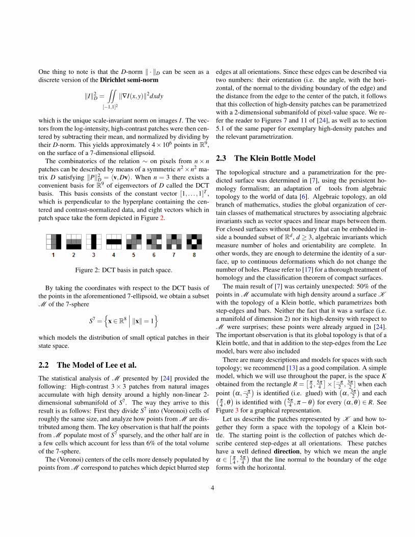
D = 〈v,Dv〉. When n = 3 there exists aconvenient basis for R9 of eigenvectors of D called the DCTbasis. This basis consists of the constant vector [1, . . . ,1]T ,which is perpendicular to the hyperplane containing the cen-tered and contrast-normalized data, and eight vectors which inpatch space take the form depicted in Figure 2.

Figure 2: DCT basis in patch space.

By taking the coordinates with respect to the DCT basis ofthe points in the aforementioned 7-ellipsoid, we obtain a subsetM of the 7-sphere

S7 ={

x ∈ R8∣∣∣ ‖x‖= 1

}which models the distribution of small optical patches in theirstate space.

2.2 The Model of Lee et al.The statistical analysis of M presented by [24] provided thefollowing: High-contrast 3× 3 patches from natural imagesaccumulate with high density around a highly non-linear 2-dimensional submanifold of S7. The way they arrive to thisresult is as follows: First they divide S7 into (Voronoi) cells ofroughly the same size, and analyze how points from M are dis-tributed among them. The key observation is that half the pointsfrom M populate most of S7 sparsely, and the other half are ina few cells which account for less than 6% of the total volumeof the 7-sphere.

The (Voronoi) centers of the cells more densely populated bypoints from M correspond to patches which depict blurred step

edges at all orientations. Since these edges can be described viatwo numbers: their orientation (i.e. the angle, with the hori-zontal, of the normal to the dividing boundary of the edge) andthe distance from the edge to the center of the patch, it followsthat this collection of high-density patches can be parametrizedwith a 2-dimensional submanifold of pixel-value space. We re-fer the reader to Figures 7 and 11 of [24], as well as to section5.1 of the same paper for exemplary high-density patches andthe relevant parametrization.

2.3 The Klein Bottle Model

The topological structure and a parametrization for the pre-dicted surface was determined in [7], using the persistent ho-mology formalism; an adaptation of tools from algebraictopology to the world of data [6]. Algebraic topology, an oldbranch of mathematics, studies the global organization of cer-tain classes of mathematical structures by associating algebraicinvariants such as vector spaces and linear maps between them.For closed surfaces without boundary that can be embedded in-side a bounded subset of Rd , d ≥ 3, algebraic invariants whichmeasure number of holes and orientability are complete. Inother words, they are enough to determine the identity of a sur-face, up to continuous deformations which do not change thenumber of holes. Please refer to [17] for a thorough treatment ofhomology and the classification theorem of compact surfaces.

The main result of [7] was certainly unexpected: 50% of thepoints in M accumulate with high density around a surface Kwith the topology of a Klein bottle, which parametrizes bothstep-edges and bars. Neither the fact that it was a surface (i.e.a manifold of dimension 2) nor its high-density with respect toM were surprises; these points were already argued in [24].The important observation is that its global topology is that of aKlein bottle, and that in addition to the step-edges from the Leemodel, bars were also included

There are many descriptions and models for spaces with suchtopology; we recommend [13] as a good compilation. A simplemodel, which we will use throughout the paper, is the space Kobtained from the rectangle R =

[π

4 ,5π

4

]× [−π

2 , 3π

2 ] when eachpoint

(α, −π

2

)is identified (i.e. glued) with

(α, 3π

2

)and each(

π

4 ,θ)

is identified with( 5π

4 ,π−θ)

for every (α,θ) ∈ R. SeeFigure 3 for a graphical representation.

Let us describe the patches represented by K and how to-gether they form a space with the topology of a Klein bot-tle. The starting point is the collection of patches which de-scribe centered step-edges at all orientations. These patcheshave a well defined direction, by which we mean the angleα ∈

[π

4 ,5π

4

)that the line normal to the boundary of the edge

forms with the horizontal.

4

Figure 3: Klein bottle model K. (α,−π/2) is identified with(α,3π/2) and (π/4,θ) is identified with (5π/4,π−θ) for ev-ery (α,θ). Arrows of the same color describe the gluing rules.

Figure 4 shows patches from centered step-edges at various ori-entations.

Figure 4: Patches from step-edges at various orientations. Thetwo patches on the far left column have direction α = π .

As the reader might guess, direction will correspond to thefirst coordinate in the model K. The next and final step is toadd to the Klein bottle manifold those patches which corre-spond to non-centered step-edges and bars. Consider for a fixedα ∈

[π

4 ,5π

4

)the centered step-edges E and −E, the centered

dark bar B (i.e. the patch of the form light-strip |dark-strip |light-strip) and the light bar −B, all of which have direction α .The definition of direction for bars is analogous to that of step-edges. Moving along the vertical coordinate in the Klein bottlemodel K (Figure 3) corresponds to the transitions

(−B) =⇒ E =⇒ B =⇒ (−E) =⇒ (−B)

parametrized by

cos(θ)E + sin(θ)B, for θ ∈[−π

2,

3π

2

).

We show in figure 5 these four transitions for the case α = π .

Figure 5: Transitions from bars to edges with direction α =π . The transition is parametrized by cos(θ)E + sin(θ)B forθ ∈

[−π

2 , 3π

2

). The top row, from left to right, corresponds to

θ going from −π/2 to 0. Subsequent rows correspond to theintervals

(0, π

2

],(

π

2 ,π]

and(π, 3π

2

], respectively.

This completes the description of the Klein bottle manifold offrequently occurring patches. In summary, K is comprised ofpatches depicting step-edges and bars at all orientations. Thesepatches can be parametrized via their direction α , and theiredge/bar structure given by the transition angle θ . When wetake into account the identifications, i.e. the fact that differ-ent pairs (α,θ) might describe the same patch (e.g. both

(π

4 ,0)

and( 5π

4 ,π)

describe the centered step-edge with gradient in thenortheast direction), then the model K (Figure 3) emerges. Weshow in Figure 6 a lattice of elements from K , arranged ac-cording to their coordinates (α,θ) ∈ K. From this arrangementit readily follows that these patches fit together in a space withthe topology of a Klein bottle.

Remark 2.1. For (α,θ) ∈ K let a+ ib = eiα and c+ id = eiθ .Let p be the polynomial

p(x,y) = c(ax+by)

2+d

√3(ax+by)2

4(1)

and let P = [pi j] be the 3×3 patch obtained via local averaging

pi j =∫ −2i+5

3

−2i+33

∫ 2 j−33

2 j−53

p(x,y) dxdy, i, j = 1,2,3.

It follows that each (α,θ) ∈ K determines a unique patch P,and that by taking entry-wise logarithms, centering and D-normalizing P we get a unique element in K . This impliesthat K can be parametrized via the set of polynomials given byequation 1 satisfying a2 +b2 = c2 +d2 = 1.

Remark 2.2. Relevant to our discussion of the distribution oflocal features from natural images, is the solid of second orderlocal image structure introduced by [15]. The aforementioned

5

Figure 6: A lattice of patches in K . The first coordinate α

measures direction, and the second coordinate θ measures thebar/edge structure.

solid is a 3-dimensional orbifold (i.e. the set of orbits from agroup acting on a manifold) constructed as follows: Let I(x,y)be an image and consider, for a fixed scale σ > 0, the 2nd orderjet at (x0,y0). That is, the vector[

c00 c10 c01 c20 c11 c02]

(2)

resulting from the L2-inner product of I(x− x0,y− y0) with

G(n,m)σ (x,y) =

1σ22π

(dn

dxn e−x2

2σ2

)(dm

dym e−y2

2σ2

)for n,m = 0,1,2. The inner product with G(n,m)

σ is what we de-note by cnm, c10 and c01 encode the 1D local (blurred-edge-like)structure, while c20 and c02 measure the pure 2D (centered bar)behavior. The space of 2nd order jets is the set of vectors ofthe form (2) one obtains by varying both (x0,y0) and I. Now,every time an image is translated, rotated or reflected, an in-tensity constant is added or image intensity is multiplied by apositive factor, then a corresponding transformation (which onecan write down explicitly) is applied to its jets. Thus, we canregard these transformations as acting on jet space itself. In thissetting, two jets are said to be in the same orbit if one can beobtained from the other by a sequence of such transformations.

The solid defined by [15] is the set of orbits from the spaceof 2nd order jets via the action of the aforementioned group of

transformations. In a nutshell, points in this space describe (upto 2nd order) the local structure of an image in a way whichis invariant to rotations, translations, reflections, and alterationsof intensity or contrast by a constant factor. A major feature ofthis highly-curved object is that it can be realized, in a volume-preserving manner, as a subset of R3, which in turn allows oneto study the distribution of 2nd order features from ensemblesof images. For natural images, in particular, it is shown that 1Dlocal forms (i.e. edge-like) are overly represented: 50% of thedistribution is concentrated in 20% of the volume of the solid.

2.4 The Relevance of Projecting onto the KleinBottle

The prominence of bars and edges as image primitives has beenextensively documented. At the physiological level it is knownthat the visual cortex in cats and macaque feature large arrays ofneurons sensitive only to stimuli from straight lines at specificorientations [19, 20]. In information theory they arise as the fil-ters which minimize redundancy in a linear coding framework[2]; while in feature learning for image representation, bars andedges are prevalent dictionary elements ([21] and [35]).

The Klein bottle model K can thus be regarded as a code-book for two of the most important features in natural images,not only from an statistical standpoint, but from a physiologi-cal and computational one. Its continuous character allows oneto bypass the quantization problem2, yielding accurate repre-sentations, while its low intrinsic dimensionality (a 2-manifold)provides the sparseness and economy desirable in any codingscheme. Moreover, the fact that the Klein bottle can be seen asa twisted version of the torus S1×S1 (see section 3), allows oneto represent probability density functions on it with convenientbases for the space of square-integrable functions L2(K). Thisis highly non-trivial if K is replaced by other spaces.

When we project patches from an image onto their closestpoints in K , we are essentially locally labeling the image ac-cording to its localized bar/edge-like structure, while retainingthe directionality of the patch. Locally labeling images accord-ing to feature categories such as bars, blobs, edges, etc, has beenhighly successful in texture classification tasks, as shown by thework of [8]. Their success stems from having highly descriptivefeature categories at several scales, with features ranging fromthose ubiquitous across texture images (e.g. edges and bars), tothe ones which are more class-characteristic. What our frame-work provides is a way of concisely representing the ubiquitouspart, using the low-dimensional manifold in patch space whichbest describes it. And what we show in this paper, is that even

2Provided one has a “continuous projection” such as the one described insubsection 3.1

6

with this limited vocabulary it is possible to achieve high classi-fication rates. We do not claim that the Klein bottle manifold isthe right space for studying distributions of patches from textureimages, but rather that it is a good initial building block (as ourresults suggest) for a low-dimensional space (not necessarily amanifold) representing a richer vocabulary of features.

We close with a discussion of instances where it is to beexpected that relevant portions of patch-space are describedwith low-dimensional submanifolds, and how one can deter-mine their topology. It is to this framework that we refer to asTopological Dictionary Learning.

2.5 Learning the Topology of Relevant Subsetsof Patch-Space

If a set of relevant patches, e.g. in high density regions ofstate-space or with high discriminative power, can be describedwith a few attributes having some form of symmetry, thenthe existence of a low dimensional geometric object whichparametrizes them is to be expected. In this case, the topologyof the underlying space can be uncovered using the persistenthomology formalism [6], while the parametrization step can beaided with methods such as Circular Coordinates [10] or theTopological Nudged Elastic Band3.

The Klein bottle model K presented by [7] was indeed thefirst realization of the Topological Dictionary Learning pro-gram, but other features can be also succinctly described. Asan example, let us consider the set of n× n patches depictingbars as the ones in Figure 7.

Figure 7: 7× 7 patches in gray scale depicting bars at severalpositions and orientations.

One way of thinking about these patches is as the set of linesin R2, union an extra point representing the empty (all white)patch. Notice that each line is determined by its orientation anddistance to the origin. For a parametrization, let us consider the

3Preprint available at http://arxiv.org/abs/1112.1993

upper hemisphere of S2 in spherical coordinates

x = sin(φ)cos(θ)y = sin(φ)sin(θ) 0≤ φ ≤ π

2 and 0≤ θ < 2π

z = cos(φ)

and let (φ ,θ) describe a patch P as follows : If 0 < φ ≤ π

2 , letP correspond to the line ` in R2 with parametric equation

`(t) = t

−sin(θ)

cos(θ)

+ cot(φ)

cos(θ)

sin(θ)

.If φ = 0, then let P be the constant patch. If we flatten the up-per hemisphere of S2 so that we get a disk, and place on eachpolar coordinate (z,θ) the patch one obtains, then it followsthat the constant patch will be at the center of the disk, andpatches representing lines through the origin will be exactly atthe boundary z = 1. Another thing to notice is that (1,θ) yieldsthe same patch as (1,θ +π), and that no other duplications oc-cur. In summary, the set of n×n patches depicting lines at dif-ferent orientations and positions, along with the constant patch,can be parametrized via a 2-dimensional disk where boundarypoints have been identified with their antipodals. Thus, the un-derlying space is the real projective plane RP2, a 2-dimensionalmanifold inside pixel-value space Rn2

. Notice that not only dowe get a considerable reduction in dimensionality, but the factthat RP2 can be modeled as a quotient of S2 allows one to ap-ply geometric techniques from the 2-sphere, to sets of patchesdepicting lines.

As we have seen, sets of patches which can be described interms of a few geometric features can often be para- metrizedwith low dimensional objects embedded in pixel-value space.Next we will concentrate on the Klein bottle dictionary K , andon how to use it in the representation of distributions of patchesfrom texture images.

3 Representing K-DistributionsGiven a digital image in gray scale, it follows from the previoussection that most of its n×n patches can be regarded as pointsin Rn2

close to K . This is the case if n is small with respectto the scale of features in the image, and if “most” refers to thenon-constant patches exhibiting a prominent directional pattern.These points, in Rn2

, can be projected onto K yielding a finiteset S ⊂ K, which can be interpreted as a random sample froman underlying probability density function f : K −→R. We willrefer to such an S as a K-sample, and to its associated f as its K-distribution. Assuming that f is square integrable over K, and

7

given an orthonormal basis {φk}k∈N for L2(K,R), there exists aunique sequence of real numbers { fk}k∈N so that

f =∞

∑k=1

fkφk. (3)

Moreover since ‖ f‖2L2 =

∞

∑k=1

f 2k , then given ε > 0 there exists

J ∈ N so that k ≥ J implies | fk| < ε , and therefore the vector( f1, . . . , fJ) can be regarded as a way of representing (an ap-proximation to) the distribution of n×n patches from the origi-nal image.

The representation for K-distributions we propose in this pa-per is an estimate of the vector ( f1, . . . , fJ) from the K-sampleS⊂ K. The basis for L2(K,R) will be derived from the trigono-metric basis einθ for L2(T), where T denotes the circle R/2πZ.Notice that using approximations via step functions, instead ofcomplex exponentials, recovers a histogram representation (seeRemark 3.13).

We will show in this section how to go from an image to theK-sample S ⊂ K, how to construct bases for L2(K), and thenhow to estimate the coefficients f1, . . . , fJ from S. We show thatthe estimators for the fk’s can be chosen to be unbiased andwith convergence almost surely as |S| → ∞ (Theorem 3.12);that taking finitely many coefficients for our representation isnearly optimal with respect to mean square error; and that when{φk}k∈N is derived from the trigonometric basis einθ , then im-age rotation changes our representation via an specific lineartransformation (Theorem 3.15).

3.1 From images to K-samplesGiven an n× n patch P = [pi j] from a digital image in grayscale, we can think of it as coming from a differentiable (oralmost-everywhere differentiable) intensity function

IP : [−1,1]× [−1,1]−→ R

via local averaging

pi j =

1− 2i−2n∫

1− 2in

−1+ 2 jn∫

−1+ 2 j−2n

IP(x,y)dxdy

That is, each pixel is the result of integration of light intensityover some finite area. In this context, we will refer to IP as anextension of P.

We say that a patch P is purely directional if there exist an

extension IP of P, a unitary vector[

ab

]∈ R2 and a function g :

R−→R such that IP(x,y) = g(ax+by) for every x,y ∈ [−1,1].The Klein bottle model K we have presented, can therefore beunderstood as the set of purely directional patches in which g isa degree 2 polynomial without constant term, and so that IP isunitary with respect to the Dirichlet semi-norm

‖IP‖2D =

∫∫[−1,1]2

‖∇IP‖2dxdy.

This interpretation allows us to formulate our two-step strategyfor projecting a given patch onto K:

1. Find a unitary vector[

ab

]which in average is the most

parallel to ∇IP. This way, IP will be as constant as possible

in the[−ba

]direction.

2. Let the projection of P onto K (hence K), be the patchcorresponding to the polynomial

p(x,y) = c(ax+by)

2+ d

√3(ax+by)2

4,c2 +d2 = 1

which is closest to IP(x,y) as measured by ‖ · ‖D.

Let us see how to carry this out. If IP is an extension of Pthen we have the associated quadratic form

QP(v) =∫∫

[−1,1]2

〈∇IP(x,y),v〉2dxdy. (4)

Since 〈∇IP(x,y),v〉2 is maximized as a function of v unitary, at(x,y), when v is parallel to ∇IP(x,y), then maximizing QP is infact equivalent to finding the vectors which in average are themost parallel to ∇IP.

Proposition 3.1. Let P be a patch, IP an extension and let QPbe the associated quadratic form (equation 4), which we writein matrix form as QP(v) = vT APv for AP symmetric.

1. If P is purely directional and IP(x,y) = g(ax+by), for a2+b2 = 1, then

QP

([ab

])= max‖v‖=1

QP(v)

2. Let Emax(AP)⊂R2 be the eigenspace corresponding to thelargest eigenvalue of AP. If S1 ⊂ R2 is the unit circle, thenEmax(AP)∩S1 is exactly the set of maximizers for QP overS1.

8

3. If the eigenvalues of AP are distinct, then

Emax(AP)∩S1 = {vP,−vP},

which determines a unique αP ∈ [π/4,5π/4) so that

{vP,−vP}= {eiαP ,−eiαP}.

Remark 3.2. We would like to point out that Proposition 3.1 isclosely related to the well-known corner detector by [16]. If welet x1 := x and x2 := y, then the entries in the matrix AP can bewritten explicitly as

AP(i, j) =∫∫

[−1,1]

∂ IP

∂xi

∂ IP

∂x jdxdy, i, j = 1,2.

This is exactly the matrix in the Harris-Stephens corner detec-tor. Recall that according to [16], if λ1,λ2 are the eigenvaluesof AP then P is a flat region if both eigenvalues are small, it isa corner if both eigenvalues are large, and an edge if one of theeigenvalues is much larger than the other. Since

λ1 +λ2 = trace(AP) = ‖IP‖2D = 1 and λi ≥ 0

then by requiring λ1 6= λ2, we are essentially imposing the ex-istence of a larger eigenvalue and thus we remove the patchesdepicting corners and flat regions, from the sample to be pro-jected onto the Klein bottle.

Proposition 3.3. Let a+ ib = eiα for α ∈ R, and let

〈 f ,g〉D =∫∫

[−1,1]2

〈∇ f (x,y),∇g(x,y)〉dxdy

denote the inner product inducing the Dirichlet semi-norm ‖ ·

‖D. If u = (ax+by)2 . Then the vector

[c∗

d∗

]∈ S1 which minimizes

the ‖ · ‖D-error

Φ(c,d) =∥∥∥IP−

(cu+d

√3u2)∥∥∥

D, c2 +d2 = 1

is given by

c∗ =〈IP,u〉D√

〈IP,u〉2D +3〈IP,u2〉2D

d∗ =

√3〈IP,u2〉D√

〈IP,u〉2D +3〈IP,u2〉2D

whenever

ϕ(IP,α) = 〈IP,u〉2D + 〈IP,u2〉2D 6= 0

and it determines a unique θP ∈ [−π/2,3π/2) so thatc∗+ id∗ = eiθP .

The association P 7→ (αP,θP) ∈ K, with αP as in Proposi-tion 3.1 and θP as in Proposition 3.3, is well-defined up to aconsistent choice of an extension IP, or rather that of its gra-dient ∇IP. The choice we make in this paper is to let ∇IP bepiecewise constant and equal to the discrete gradient of P. Thespecifics on how to compute this gradient, how to deal with thecase in which AP is a scalar matrix, and what to do when theminimizer for Φ(c,d) is not well defined, will be discussed inthe Implementation Details subsection (4.2).

Let us say a few words regarding the sense in which

P 7→ (αP,θP) ∈ K

is considered a projection. The orthogonal projection onto alinear subspace of an inner product space is uniquely charac-terized by its distance minimizing property. While K is not alinear subspace of Rn2

, the approximation

IP ≈ c(ax+by)

2+d

√3(ax+by)2

4

attempts to minimize the ‖·‖D-error as described in Proposition3.3. It is because of this property that P 7→ (αP,θP) is referredto as the projection of P onto K.

Our labelling scheme P 7→ (αP,θP) ∈ K can be interpreted,at a given scale, as a continuous version of the MR8 (MaximumResponse 8, see Figure 8) representation [35], that omits theGaussian filter and its Laplacian.

Figure 8: The MR8 (Maximum Response 8) filter banks. Bytaking the maximum filter response (or projection) across eachcolumn, the MR8 represents a patch in terms of eight real num-bers.

Indeed, at each one of three scales, the MR8 representa-tion registers the maximum projection (or filter response) of apatch onto six rotated versions of a linear (vertical edge) and aquadratic (vertical bar) filter, yielding the first six out of eightnumbers in the descriptor. The last two, are the responses to aGaussian and to the Laplacian of a Gaussian. The Klein bottlerepresentation on the other hand, takes into account all possi-ble rotations of the linear and quadratic filters, and also retains

9

the maximizing direction. In contrast to the MR8, we make ourdescriptor rotation invariant not by collapsing the directionalcoordinate, but by determining the effect on both the projectedsample S ⊂ K and the estimated Fourier-Like coefficients, asone rotates the image (Theorem 3.15). Once this is understood,one can make the distance between the descriptors invariant tothe effects of rotation.

Another difference between our method and the MR8 repre-sentation is the way in which scale is handled. On the one hand,the MR8 filter keeps the size of the patch fixed, but changes theinner resolution via convolution with Gaussian kernels. Indeed,computing the filter response of a patch to the k-th derivativeof a Gaussian is the same as first blurring the patch with theGaussian, changing the scale, and then computing the L2-innerproduct with a degree k Hermite polynomial. See for instancesection 1.4 of [14]. We would like to point out that this fallswithin the multi-scale representation of Gaussian scale-spacetheory of [22].

[27] have studied the distribution in scale-space of smallpatches from natural images via 3-jet representations. Again,they provide evidence for the existence of a highly-nonlinearsurface in jet-space, parametrizing multi-scale blurred step-edges. We believe the results of topological dictionary learn-ing and density representation presented in this paper can beadapted to this scale-space framework. We hope to pursue theseideas in future work, but for the moment we use a simple multi-scale representation. In general terms, and in contrast to theMR8 representation, we increase the patch size; for each patchsize we obtain a distribution, we estimate its coefficients, andthen concatenate them to obtain a multi-scale representation.Please refer to section 4.2 for further details.

3.2 Constructing Bases for L2(K)

The problem of finding good orthonormal bases for L2(M)when (M,η) is a general measure space, is in fact a very dif-ficult one. For even when there are theoretical guarantees fororthonormal bases to exist, it is highly nontrivial to make prin-cipled choices. It is at this point that having the Klein bottleas underlying space ceases to be just an interesting feature andbecomes a crucial component of our analysis. As we will seeshortly, the Klein bottle is one space for which there are conve-nient choices of bases for L2(K).

One of the most fundamental results in the theory of square-integrable periodic functions is Fourier’s theorem, stating thatthe set {einα : n ∈ Z} of complex exponentials is an orthonor-mal basis for L2(S1). Here S1 = {z ∈ C : |z| = 1}, and it read-ily follows that {einα+imθ : n,m ∈ Z} is an orthonormal basisfor L2(T ), where T = S1×S1 denotes the 2-dimensional torus.

In other words, it is possible to choose convenient bases forL2(S1), including but not limited to trigonometric exponentials,and these in turn yield bases for L2(T ). The main point now isthat since the Klein bottle K can be recovered from T via simpleidentifications based on symmetries, as we will see next, thenfinding orthonormal bases for L2(K) amounts to doing so forL2(T ) while keeping track of said identifications.

The aforementioned symmetries arise naturally from themodels we have for the Klein bottle of edge-like and bar-like frequently occurring patches. Indeed, it follows from theparametrization of K via the set of polynomials

p(x,y) = c(ax+by)

2+ d

√3(ax+by)2

4

with a2 + b2 = c2 + d2 = 1 (see Remark 2.1), that each (z,w)in T determines a unique element in K , and that (z,w) and(z′,w′) yield the same patch if and only if one has that (z′,w′) =(−z,−w). Here w denotes the complex conjugate of w. Thatis, K (and therefore K) can be modeled as the space obtainedfrom T by identifying (z,w) with (−z,−w) for every (z,w)∈ T .Thus, in essence, one can interpret K as{{

(z,w),(−z,−w)}

: (z,w) ∈ T}

and think of elements in L2(K) as square-integrable functionsf : T −→ C satisfying the identity

f (z,w) = f (−z,−w) (5)

for every (z,w)∈ T . The reason why we think of these relationsas symmetries is explained in Figure 9.

Figure 9: The transformation µ(z,w)= (−z,−w) can be writtenin polar coordinates as µ(α,θ) = (α + π,π − θ) mod 2π . Inparticular, it maps the letter “q” on the upper left to the “d”on the lower right. The set

{{(z,w),µ(z,w)} | (z,w) ∈ T

}can

be identified with [π/4,5π/4]× [−π/2,3π/2] along with thegluing rules depicted by the arrows. This recovers the model K.

10

Notice that this characterization allows one to interpret L2(K)as a linear subspace of L2(T ). This leads one to consider theorthogonal projection

Π : L2(T )−→ L2(K)

of L2(T ) onto L2(K), which in turn yields a recipe for producingorthonormal bases for L2(K) from those of L2(T ). We describethis recipe in what follows. Firstly, an explicit formula for Π

can be derived from equation 5. Indeed,

Proposition 3.4. The function

Π : L2(T ) −→ L2(K)

g 7→ g(z,w)+g(−z,−w)2

(6)

is the orthogonal projection of L2(T ) onto L2(K).

Notice that if {φk|k ∈ N} is a basis (or a spanning set) forL2(T ) then {Π(φk)|k ∈ N} spans L2(K) and hence contains abasis. Moreover, applying Gram-Schmidt allows one to turnthis basis into an orthonormal one. In other words, any or-thonormal basis for L2(T ) yields one for L2(K). A less obviousobservation, whose proof can be found in the appendix, is thatevery orthonormal basis for L2(K) can be obtained from one ofL2(T ) in this fashion. We summarize the previous discussion inthe following theorem.

Theorem 3.5. If {φk | k ∈ N} is a spanning set for L2(T ) then

S =

{φk(z,w)+φk(−z,−w)

2

∣∣ k ∈ N}

is a spanning set for L2(K).If B ⊂S is a basis for L2(K), then applying Gram-Schmidt

to B yields an orthonormal basis for L2(K). Moreover, any or-thonormal basis for L2(K) can be recovered from one of L2(T )in this fashion.

Remark 3.6. Since bases for L2([0,1]), such as Wavelets orLegendre polynomials, can be modified to yield bases forL2(S1) and thus for L2(T ), then the previous theorem gives away of constructing lots of bases for L2(K).

In particular we have,

Corollary 3.7. Let {φn}n∈N be a basis for L2(S1). Then inpolar coordinates

{φn(α)φm(θ) | n,m ∈ N}

is a basis for L2(T ) and therefore{φn(α)φm(θ)+φn(α +π)φm(π−θ)

2

∣∣∣ n,m ∈ N}

is a spanning set for L2(K).

The next two results are perhaps the most relevant for therest of the paper; they yield Fourier-like bases for L2(K) andL2(K,R) by applying the previous corollary to the set {φk(α) =eikα}k∈Z.

Corollary 3.8. Let n ∈ Z and m ∈ N∪ {0}. Then the set offunctions

einα+imθ +(−1)n+meinα−imθ

2, m = 0 implies n is even.

is an orthonormal basis for L2(K). We refer to this set as thetrigonometric basis for L2(K).

When restricted to real valued functions f : K −→ R, one canstart with the basis B for L2(T,R) consisting of functions of theform φ(nα)ψ(mθ) where φ and ψ are either sines or cosines,and consider Π(B). This yields

Corollary 3.9. Let n,m ∈ N and let πn,m = (1−(−1)n+m)π4 . Then

the set of functions

1,√

2cos(mθ −π0,m) ,√

2cos(2nα),√

2sin(2nα),

2cos(nα) · cos(mθ −πn,m) , 2sin(nα) · cos(mθ −πn,m)

is an orthonormal basis for L2(K,R). We refer to this set as thetrigonometric basis for L2(K,R).

Remark 3.10. The symmetries which allow us to regard L2(K)as a subspace of L2(T ) (equation 5) have a simplifying effecton the inner product 〈·, ·〉T when restricted to L2(K). Indeed, iff ,g ∈ L2(K) then one can check that

〈 f ,g〉T =1

(2π)2

∫ 3π2

−π2

∫ 9π4

π4

f (α,θ)g(α,θ)dαdθ

=1

2π2

∫ 3π2

−π2

∫ 5π4

π4

f (α,θ)g(α,θ)dαdθ

and thus L2(K) can be endowed with its own inner product:

〈 f ,g〉K :=1

2π2

∫ 3π2

−π2

∫ 5π4

π4

f (α,θ)g(α,θ)dαdθ . (7)

Definition 3.11. Let f ∈ L2(K,R), 〈·, ·〉K as in equation 7, andlet

am = 〈 f ,√

2cos(mθ −π0,m)〉Kbn = 〈 f ,

√2cos(2nα)〉K

cn = 〈 f ,√

2sin(2nα)〉Kdn,m = 〈 f ,2cos(nα)cos(mθ −πn,m)〉Ken,m = 〈 f ,2sin(nα)cos(mθ −πn,m)〉K

11

be the coefficients of f with respect to the trigonometric ba-sis for L2(K,R). If we order them with respect to their (total)frequencies and alphabetic placement as

a1, a2, b1, c1, d1,1, e1,1︸ ︷︷ ︸frequency=2

, a3, d1,2, d2,1 ,e1,2, e2,1︸ ︷︷ ︸frequency=3

, a4, b2, . . .

then we get the ordered sequence KF ( f ), which we will re-fer to as the K-Fourier coefficients of f . We will denote byKFw( f ) the truncated sequence of K-Fourier coefficients con-taining those terms with frequencies less than or equal to w∈N.

3.3 Estimation in the Frequency DomainWe now turn our attention to the last step in the representa-tion scheme: Given an orthonormal basis {φk}k∈N for L2(K),f ∈ L2(K) a probability density function on K, and S ⊂ K arandom sample drawn according to f , estimate the coefficientsfk = 〈 f ,φk〉K from S. It turns out that this problem can be solvedin great generality: For any measure space (M,η) so that L2(M)has orthonormal bases with at most countably many elements,one can choose unbiased estimators for the coefficients fk. Invery general terms, what one does is to put a Dirac mass at eachpoint of S, interpret this construction as the Gaussian kernel es-timator [30] with infinitely small width, and then calculate itscoefficients with respect to the basis {φk}k∈N.

Let us motivate the definition of these estimators with thecase M = Rd and {hα | α ∈ Nd} the harmonic oscillator wavefunctions on Rd . Let S (Rd) be the set of rapidly decreas-ing complex valued functions on Rd (see [28]), S ′(Rd) itsalgebraic dual (the space of tempered distributions) and lethα : Rd −→ R be given by

hα(x1, . . . ,xd) = hα1(x1) · · ·hαd (xd).

Here α = (α1, . . . ,αd) ∈Nd and hk is the k-th Hermite functionon R. It is known that {hα | α ∈ Nd} is an orthonormal basisfor L2(Rd) (Lemma 3, page 142, [28]), and that for every T ∈S ′(Rd) the series

∑α

T (hα)hα

converges 4 to T . This suggests we define T (φk) as the coeffi-cients of a tempered distribution T with respect to an arbitraryorthonormal basis {φk}k∈N for L2(Rd).

Now, the Dirac delta function centered at c ∈ Rd

δ (x− c) : S (Rd) −→ Cψ 7→ ψ(c)

4Convergence is with respect to the weak-* topology. This result is a conse-quence of the N-representation theorem (V.14, page 143, [28])

is a continuous linear functional and therefore an element inS ′(Rd). An application of integration by parts shows that forevery ψ ∈S (Rd) one has

limk→∞

∫Rd

ψ(x)k√πd

e−k2‖x−c‖2 dη(x) = ψ(c)

and therefore δ (x−c) is a weak limit of Gaussians with mean c,as the variance approaches zero. What this result tells us is thatδ (x− c) can be interpreted as the generalized function bound-ing unit volume, which is zero at x 6= c and an infinite spike at c.Moreover, if X1, . . . ,XN are i.i.d. (independent and identicallydistributed) random variables with probability density functionf ∈ L2(Rd ,R), then as a “generalized statistic”

fδ (X) :=1N

N

∑n=1

δ (X−Xn)

can be thought of as the Gaussian kernel estimator (see [30])with infinitely small width. The coefficients of fδ with respectto the Hermite basis can be computed as

fδ (hα) =1N

N

∑n=1

hα(xn)

and motivate the following estimation theorem.

Theorem 3.12. Let (M,η) be a measure space so that L2(M)has an orthonormal basis {φk}k∈N. If f : M −→ R is a proba-bility density function with

f =∞

∑k=1

fkφk

and X1, . . . ,XN are i.i.d. random variables distributed accord-ing to f , then

fk :=1N

N

∑n=1

φk(Xn)

is an unbiased estimator for fk. Moreover, fk converges almostsurely to fk as N→ ∞.

Proof. To see that the estimators are unbiased, notice that foreach k ∈ N the expected value of fk is given by

E[ fk] =1N

∫M

f ·N

∑n=1

φk dη =∫M

f ·φk dη = fk.

The convergence result is exactly the statement of the StrongLaw of Large Numbers.

12

Remark 3.13. Our formalism of estimated coefficients also re-covers histogram representations. Indeed, let A ⊂ [0,1] andconsider the (indicator) function 1A : [0,1] −→ R which forx ∈ [0,1] is defined as 1 if x ∈ A, and 0 otherwise. A step func-tion is any expression of the form

s(x) =m

∑i=1

ri1Ai(x)

where ri ∈ R is nonzero and the Ai’s are disjoint subintervalsof [0,1]. In the same way as the integral of a function canbe approximated via Riemann sums, one has that the set ofstep functions is dense in L2([0,1]). This means that for anyε > 0 and any f ∈ L2([0,1]) there exists a step function s sothat ‖ f − s‖L2 < ε . Fix f ∈ L2(K), ε > 0 and let s be a stepfunction no more than ε away from f . Let A1, . . . ,Am be thesubintervals of [0,1] which define s. Since the Ai’s are disjoint,it follows that the functions 1A1 , . . . ,1Am are mutually orthogo-nal in L2([0,1]) and hence can be extended, as a linearly inde-pendent set, to an orthogonal basis 1A1 , . . . ,1Am ,φm+1,φm+2 . . .of L2([0,1]). Thus, we can write

f (x) =m

∑i=1

fi1Ai(x)√|Ai|

+∞

∑j=m+1

f jφ j(x)

where |Ai| denotes the length of the interval Ai and the φ j can beassumed to have unit norm. If f is a density function on [0,1]and S = {x1, . . . ,xN} ⊂ [0,1] is drawn according to f , then The-orem 3.12 implies that one can estimate the first m coefficientsf1, . . . , fm (which describe f with accuracy ε) as

fi =1N

N

∑n=1

1Ai(xn)√|Ai|

=ni

N√|Ai|

, i = 1, . . . ,m

Here ni denotes the number of points from the sample S whichlie inside the interval Ai. In other words, the vector of esti-mated coefficients ( f1, . . . , fm), with respect to the aforemen-tioned basis, is exactly the normalized histogram on the inter-vals A1, . . . ,Am. Notice that approximation with step functionsmakes sense for any bounded space; in particular on the Kleinbottle K.

Definition 3.14. Let KF ( f ) denote the sequence of estima-tors obtained from Theorem 3.12 and the trigonometric basisfor L2(K,R). Let KF w( f ) denote the truncated sequence cor-responding to frequencies less than or equal to w ∈ N. Givena random sample S = {(α1,θ1), . . . ,(αN ,θN)} ⊂ K drawn ac-cording to f ∈ L2(K,R), we let KF ( f ,S) denote the sequence

of estimated K-Fourier coefficients

am =1N

N

∑k=1

√2cos(mθk−π0,m)

bn =1N

N

∑k=1

√2cos(2nαk)

cn =1N

N

∑k=1

√2sin(2nαk)

dn,m =1N

N

∑k=1

2cos(nαk)cos(mθk−πn,m)

en,m =1N

N

∑k=1

2sin(nαk)cos(mθk−πn,m)

and let KF w( f ,S) be its truncated version.

Now that we have established some properties of the estima-tors, let us end this section with a discussion on why truncatingthe sequence of coefficients is justified. It is the case that whilethere are reasonably good estimators for the coefficients of f invery general settings, their dependency on the choice of basismakes it hard to identify just how much information is effec-tively encoded in this representation. Let us try to make thisidea more transparent. The first thing to notice is that the se-quence of estimators

SJ( fδ ) :=J

∑k=1

fkφk

does not converge to f but to fδ (in the weak-* topology) asJ→ ∞, regardless of the sample size N, and provided we havepointwise convergence

∑k

ψkφk(x) = ψ(x), for all ψ ∈S (Rd) and all x ∈ Rd .

This is true for instance in the case of Hermite functions andtrigonometric polynomials. More specifically, what Theorem3.12 provides is a way of approximating a linear combinationof delta functions instead of the actual function f , and thus evenwhen the fk are almost surely correct for large N, the conver-gence in probability is not enough to make them decrease fastenough as k gets larger. In short, taking more coefficients isnot necessarily a good thing, so one should choose bases inwhich the first coefficients carry most of the information mak-ing truncation not only necessary but meaningful. Moreover, itis known [36] that truncation is also nearly optimal with respectto mean integrated square error (MISE) within a natural classof statistics for f . Indeed, if within the family of estimators

f ∗N :=∞

∑k=1

λk(N) fkφk

13

one looks for the sequence {λk(N)}k∈N that minimizes

MISE := E[‖ f ∗N− f‖2

2]

then provided the fk for k ≤ J(N) are large compared to var(φk)N

and the fk for k > J(N) are negligible, then letting λk(N) = 1for k ≤ J(N) and zero otherwise achieves nearly optimal meansquare error.

The previous discussion yields yet another reason for con-sidering trigonometric polynomials: The high-frequency K-Fourier coefficients tune the fine scale details of the series ap-proximation. Thus, most of the relevant information in theprobability density function is encoded in the low frequencies,which can be easily approximated via estimators that convergealmost surely as the sample size gets larger, and achieve nearlyoptimal mean square error within a large family of estimators.

3.4 The Effect of Image Rotation

We will show in what follows that image rotation has a partic-ularly simple effect on the distribution of patches on the Kleinbottle and that, with respect to the trigonometric basis, it hasan straightforward interpretation in the frequency domain: Alinear transformation depending solely on the angle of rotation.

Let us consider an n×n patch P from an image I. If I is ro-tated in the counterclockwise direction with respect to its centerby τ degrees, τ ∈ [−π,π], then one obtains a new image Iτ andP will be mapped to a patch Pτ . While this new patch is notexactly the same as rotating P by τ degrees, since we are takingsquare patches instead of disks, it follows that if I has a predom-inantly directional pattern with angle α in a pixel neighborhoodof P, then Pτ will have predominant direction α +τ . Moreover,the edge-like or bar-like structure of Pτ (i.e. the vertical coordi-nate in the Klein bottle model; see Figure 6) will be roughly thatof P. In summary, given that the horizontal coordinate (α) inthe model K encodes the predominant direction of a patch, andthe vertical coordinate (θ ) parametrizes its edge/bar-like struc-ture, then if (αP,θP) are the coordinates of P when projectedonto K, we have that (αP + τ,θP) approximate those of Pτ .

It is clear that taking (αP+τ,θP) as an approximation for theprojection of Pτ onto K could be inaccurate for the patches in Iwhich do not have a neighborhood where the image is predomi-nantly directional. What one expects, however, is that by takingthe collection of all patches from Iτ projected onto K, the localinaccuracies will be negligible when considering the global be-havior of the distribution. In other words, if S⊂K is the sampleobtained from patches of I and we let

Sτ = {(α + τ,θ) | (α,τ) ∈ S}

then if S ⊂ K is the sample from projected patches of Iτ wehave that Sτ and S can be thought of as sampled from the samedistribution. Let f : K −→R be the density function underlyingS. Since Sτ is obtained from S by horizontal translation on K,we have that Sτ (and therefore S) has distribution

f τ(α,θ) := f (α− τ,θ). (8)

What we will see now is that the trigonometric basis on Kis specially well suited for understanding the effect that imagerotation has on the frequency domain. Indeed,

Theorem 3.15. Let am,bn,cn,dn,m,en,m be the K-Fourier coef-ficients of f ∈ L2(K,R), and let aτ

m,bτn,c

τn,d

τn,m,e

τn,m be those of

f τ(α,θ) = f (α− τ,θ). Then we have the identities

aτm = am (9)bτ

n

cτn

=

cos(2nτ) −sin(2nτ)

sin(2nτ) cos(2nτ)

bn

cn

(10)

dτn,m

eτn,m

=

cos(nτ) −sin(nτ)

sin(nτ) cos(nτ)

dn,m

en,m

(11)

for every τ ∈ R and every n,m ∈ N. Thus, there exists a lin-ear map Tτ : `2(R) −→ `2(R) which preserves lengths, de-pends solely on τ , and so that KF ( f τ) = Tτ (KF ( f )) for everyf ∈ L2(K,R). Here `2(R) denotes the set of square summablesequences of real numbers.

This discussion can be summarized as follows: Rotating animage in the counterclockwise direction by τ degrees with re-spect to its center, operates as a translation of its distributionof patches on the Klein bottle model K horizontally by τ units.Please refer to figure 10 for an example.This shift of the sample translates into the K-Fourier coeffi-cients domain as a linear transformation Tτ , which can be de-scribed as a block diagonal matrix whose blocks are either thenumber 1, or rotation matrices which act by an angle 2nτ or nτ

depending on the particular frequencies.This description allows us to define a distance between K-

Fourier coefficients which is invariant under image rotation. In-deed, consider two images I and J, and let S,S′ ⊂ K be thesamples obtained from projecting their n× n patches onto theKlein bottle. Moreover, let f and g in L2(K,R) be the proba-bility density functions underlying S and S′, respectively. Re-call that KF w( f ,S) and KF w(g,S′) denote the truncated K-Fourier coefficients of f and g estimated from the samples Sand S′. Each rotation Iτ of I by τ , has the effect of shifting S

14

Figure 10: Top: distribution on the Klein bottle model K ofprojected 13×13 patches from the images on the bottom. Highand low density are represented using the colors red and blue,respectively. Notice that the one on the right is roughly a trans-lated version of the one on the left by π

6 , from left to right. Forthe figure on the top right, the heat appearing on the left side isexplained by the boundary identifications which give rise to theKlein bottle. Bottom: Two images of bricks.

in the horizontal direction in K by τ units yielding the sampleSτ . Since Sτ has underlying distribution f τ then we can alsocompute KF w( f τ ,Sτ), which is in essence an estimate of theK-Fourier coefficients corresponding to the rotated image Iτ .By considering the expression

dR(I,J) := infτ

∥∥∥KF w( f τ ,Sτ)− KF w(g,S′)∥∥∥

2(12)

we are in fact taking all possible rotated versions of I and J,and computing the smallest distance between their estimatedK-Fourier coefficients. In other words, among all possible pair-ings of rotated versions of I and J, we compute the smallestdistortion as measured with estimated K-Fourier coefficients. Itfollows that this distance is invariant under rotations of I and J.We would like to note that images of rotated textured objectsare also affected by the roughness of the material in the form of

local shading. For this type of rotation dR is invariant only upto a certain degree. We use a real data set (the SIPI database) ofimages of rotated textured objects in order to illustrate the be-havior of dR. Please refer to Figure 17 in Section 4.2. It is alsoimportant to note that this distance is not equipped, in principle,to deal with 3d motions and non-rigid deformations.

3.5 Implementing the dR DistanceThe most important point is not that dR exists, but that it canbe efficiently computed for truncated sequences of K-Fouriercoefficients: Using the linear transformation Tτ from Theorem3.15 we get that Tτ

(KF w( f ,S)

)= KF w( f τ ,Sτ) and therefore

equation 12 can be rewritten as

dR(I,J) = infτ

∥∥∥Tτ

(KF w( f ,S)

)− KF w(g,S′)

∥∥∥2

(13)

Moreover, since Tτ (thought of as a matrix) is made up of blocksof rotation matrices, then it does not change lengths (it is anisometry), and hence computing dR(I,J) is equivalent to maxi-mizing the inner product⟨

Tτ

(KF w( f ,S)

), KF w(g,S′)

⟩(14)

with respect to τ . Using the fact that the entries of Tτ , as amatrix, are sines and cosines of angles of the form mτ , thencomputing the derivative of equation 14 with respect to τ andmaking it equal to zero yields the following result:

Theorem 3.16. There is a nonzero complex polynomial p(z)of degree at most 2w, with coefficients depending solely onKF w( f ,S) and KF w(g,S′), and so that if τ∗ is a minimizerfor

Ψ(τ) =∥∥∥KF w( f τ ,Sτ)− KF w(g,S′)

∥∥∥2

then ξ∗ = eiτ∗ is a root of p(z).

We describe the construction of this polynomial in the proofof the Theorem, but what is important is that from S, S′, w andτ one can compute dR(I,J) by finding the roots of p(z). Theseroots can, in principle, be computed as the eigenvalues of thecompanion matrix of p(z), for which fast algorithms exist. Thisis how the MATLAB routine roots is implemented. One canthen look among the arguments of the unitary complex roots ofp(z) for the global minimizers (in [−π,π]) of equation 12.

It is known [26] that roots produces the exact eigenvaluesof a matrix within roundoff error of the companion matrix of p.This, however, does not mean that they are the exact roots of apolynomial with coefficients within roundoff error of those ofp, but the discrepancy is well understood. Indeed, let p be the

15

monic polynomial having roots(p) as its exact roots, let ε bethe machine precision and let E = [Ei j] be a perturbation matrix,with Ei j a small multiple of ε , and so that if A is the companionmatrix of p then A+E is the companion matrix of p. It follows[12] that if

p(z) = zn +an−1zn−1 + · · ·+a1z+a0

then to first order the coefficient of zk−1 in p(z)− p(z) is

k−1

∑m=0

am

n

∑i=k+1

Ei,i+m−k−n

∑m=k

am

k

∑i=1

Ei,i+m−k.

Hence even when roots(p) does not return the exact roots of p,but those of a slight perturbation p, their arguments can be usedas the initial guess in an iterative refinement such as Newton’smethod. This is how we have implemented the dR distance: Wecompute the eigenvalues of the companion matrix for p, andthen use their arguments (as complex numbers) in a refinementstep via Newton’s method on equation 14.

3.6 Rotation-Invariant K-Fourier CoefficientsWe end this section with a rotation-invariant version of our se-quence of estimated K-Fourier coefficients. In a way, it canbe thought of as a canonical representation, with respect to im-age rotation, for estimated K-Fourier coefficients. Let S ⊂ Kbe a random sample drawn according to f : K −→ R, and letKF w( f ,S) be the estimated K-Fourier coefficients. Recall thatthis is (Definition 3.14) a truncation of the ordered sequence

a1 , a2 , b1 , c1 , d1,1 , e1,1 , a3 , d1,2 , d2,1 , e1,2 , . . .

Let v =

[d1,1e1,1

]; we say that KF w( f ,S) is in canonical form

if d1,1 > 0 and e1,1 = 0. The first point is that for estimatedK-Fourier coefficients there is, in general, a value of τ so thatTτ

(KF w( f ,S)

)is in canonical form. Indeed, since ‖v‖= 0 is

a zero probability event, then there exists (with probability one)σ ∈ [0,2π) so that‖v‖

0

=

cos(σ) −sin(σ)

sin(σ) cos(σ)

v

It follows from Theorem 3.15 (equation 11) that the vectorTσ

(KF w( f ,S)

)is in canonical form. Let us change the no-

tation from σ to σ( f ) to indicate the dependence on f . Thesecond, and perhaps most important point, is that if we con-sider the estimated K-Fourier coefficients from rotated versionsof the same image, then they all have the same canonical form.Indeed,

Proposition 3.17. Let σ( f ) be as in the previous paragraph.Then σ ( f τ)≡ σ( f )− τ (mod 2π), and therefore

Tσ( f τ )

(KF ( f τ ,Sτ)

)= Tσ( f )

(KF ( f ,S)

)for every τ .

This proposition implies that the following makes sense.

Definition 3.18. Let v =

[d1,1e1,1

]and let σ( f ) ∈ [0,2π) be so

that Tσ( f )

(KF ( f ,S)

)is in canonical form. We let this vector

be the estimated sequence of rotation-invariant K-Fourier co-efficients, for a sample S⊂ K drawn according to a distributionf ∈ L2(K,R).

That is, it is well defined to regard the canonical form asa rotation-invariant version of the estimated K-Fourier coeffi-cients.

4 Results

The purpose of this section is to apply the theory we have devel-oped so far, to the problem of classifying materials from textureimages photographed under various poses and illuminations.We begin by describing the data sets which we will use: TheCUReT, KTH-TIPS and UIUCtex databases for classification,and the SIPI data set to illustrate the rotation invariant proper-ties of our descriptor.

Next we give a detailed description of the numerical imple-mentation, as well as the results on the SIPI data set. Thelast two parts deal with the metric learning approach we usefor classification, and a summary (as well as comparisons withstate-of-the-art methods) of our results.

4.1 The Data Sets

SIPI 5 The SIPI rotated textures data set, maintained by theSignal and Image Processing Institute at the University ofSouthern California, consists of 13 of the Brodatz images [5],digitized at different rotation angles: 0, 30, 60, 90, 120, 150 and200 degrees. The 91 images are 512× 512 pixels, 8 bits/pixel,in TIFF format.

5http://sipi.usc.edu/database

16

Figure 11: Exemplars from the SIPI Rotated Texture data set

CUReT 6 The Columbia-Utrecht Reflectance and Texturedatabase [9], is one of the most popular image collections usedin the performance analysis of texture classification methods.It features images of 61 different materials, each photographedunder 205 distinct combinations of viewing and illuminationconditions, providing a considerable range of 3D rigid motions.Following the usual setup in the literature, the extreme view-ing conditions are discarded, leaving 92 gray scale images permaterial, of size 200×200 pixels, 8 bits/pixel, in PNG format.What makes this a challenging data set, is both the consider-able variability within texture class, and the many commonal-ities across materials. One drawback, in terms of scope, is itslack of variation in scale.

Figure 12: The 61 materials in the CUReT data set

6http://www.cs.columbia.edu/CAVE/software/curet

KTH-TIPS 7 The KTH database of Textures under varying Il-lumination Pose and Scale, collected by Mario Fritz under thesupervision of Eric Hayman and Barbara Caputo, was intro-duced in [18] as a natural extension to the CUReT database.The reason for creating this new data set was to provide widevariation in scale, in addition to changes in pose and illumina-tion. The database consists of 10 materials (already present inthe CUReT database), each captured at 9 different scales and 9distinct poses. That is, the KTH-TIPS data set has 810 images,200×200 pixels, 8 bits/pixel in PNG format.

Figure 13: Three scales of each of the ten materials in the KTH-TIPS data set.

UIUCTex8 The UIUC Texture database, first introduced in[23], and collected by the Ponce Research Group at the Univer-sity of Illinois at Urbana-Champaign, features 25 texture classeswith 40 samples each. The challenge of this particular data setlies in its wide range of viewpoints, scales, and non-rigid defor-mations. All images are in gray scale, JPG format, 640× 480pixels, 8bits/pixel.

Figure 14: Four exemplars from each of the twenty five classesin the UIUC Texture data set.

7http://www.nada.kth.se/cvap/databases/kth-tips8http://www-cvr.ai.uiuc.edu/ponce grp/data

17

4.2 Implementation DetailsUsing the mathematical framework developed in section 3, wenow give a detailed description of the steps involved in comput-ing the estimated K-Fourier coefficients of a particular image,as well as the form of the EKFC descriptor.

Preprocessing Given a digital image in gray scale and an oddinteger n, we extract its n× n patches. The choice of n oddmakes the implementation simpler, but is somewhat arbitraryand has no bearing on the results presented here. If the imagehas pixel depth d, then each patch is an n× n integer matrixwith entries between 0 and 2d − 1. We add 1 to each entry inthe matrix, and following Weber’s law take entry-wise naturallogarithms. Each log-matrix is then centered by subtracting itsmean (as a vector of length n2) from each component, and D-normalized provided its D-norm is greater than 0.01. Otherwisethe patch is discarded for lack of contrast.

The Projection Let P be an n× n patch represented by thecentered and normalized log-matrix [pi j]. As described in thediscussion following Proposition 3.3, we let ∇IP be piecewiseconstant and equal to the discrete gradient of P, which we nowdefine. If 2≤ i, j ≤ n−1 then we let

∇P(i, j) =12

pi, j+1− pi, j−1

pi−1, j− pi+1, j

HP(i, j) =

pi, j+1−2pi, j + pi, j−1 HxyP(i, j)

HxyP(i, j) pi+1, j−2pi, j + pi−1, j

where

HxyP(i, j) =pi−1, j+1− pi−1, j−1 + pi+1,i−1− pi+1, j+1

4.

If either r ∈ {1,n} or t ∈ {1,n}, then there exists a unique(i, j) ∈ {2, . . . ,n−1}2 which minimizes |i− r|+ | j− t|, and welet

∇P(r, t) = ∇P(i, j)+HP(i, j)[

r− ij− t

].

That is, we approximate the gradient of P at a location (r, t) near(i, j) using the first order Taylor expansion. As for the gradientof the extension IP, we let ∇IP(x,y) = ∇P(i, j) if∣∣∣∣x−(−1+

2 j−1n

)∣∣∣∣+ ∣∣∣∣y−(1− 2i−1n

)∣∣∣∣< 1n

for some (i, j) ∈ {1, . . . ,n}2, and 0 otherwise. This definitioncaptures directionality more accurately than simply calculating

finite differences. This can be seen, for instance, in a 3×3 patchwith extension IP(x,y) =

√3(x+y)2

8 .If the eigenvalues of the associated matrix AP are distinct (see

Proposition 3.1), then we let αP ∈ [π/4,5π/4) be the directionof the eigenspace corresponding to the largest eigenvalue. SinceAP is a 2×2 matrix, αP can be computed explicitly in terms of∇P. If AP has only one eigenvalue, then the patch P is discardeddue to its lack of a prominent directional pattern.

If Φ(c,d) is constant (see Proposition 3.3) then P is dis-carded, since it does not have linear nor quadratic components.Otherwise we let θP ∈ [−π/2,3π/2) correspond to the min-imizer (c∗,d∗). Next we compute Φ(c∗,d∗), which can bethought of as the the distance from P to K. Notice that the trian-gular inequality with respect to ‖·‖D implies that Φ(c∗,d∗)≤ 2.We include (αP,θP) in the sample S ⊂ K if Φ(c∗,d∗) ≤ rn, forrn as reported in Table 1.

Table 1: Maximum distance to Klein bottlePatch size (n) 3 5 7 9 n≥ 11

rn 1.2247 1.3693 1.4031 1.4114 1.4135

The rationale behind this choice is as follows:∥∥∥IP−(

c∗u+d∗√

3u2)∥∥∥

D=√

2(1−ϕ(IP,αP))

and the values of rn are set so that ϕ(IP,αP)≥ 12n−1 is the inclu-

sion criterion. Here√

ϕ(IP,αP) can be thought of as the sizeof the contribution of Span

{(ax+by),(ax+by)2

}if one were

to write a series expansion for IP(x,y) in terms of the (rotated)monomials (ax+by)k(ay−bx)m, k,m ∈ N.

The K-Fourier Coefficients We select the cut-off frequencyw ∈ N so that KF w( f ,S) includes the coefficients with largevariance, and excludes the first regime where the fk tend tozero. Recall that after this regime the fk oscillate with largevariance since SJ( fδ )→ fδ . For the results presented here welet w = 6, and fix it for once and for all. While similar cut-off frequencies have been obtained with maximum likelihoodmethods, see for instance [11], other choices might improveclassification results. It follows that KF w( f ,S) is a vector oflength 42. We illustrate the computation of the estimated K-Fourier coefficients. Let us consider the K-sample from 3× 3patches in the image depicted in Figure 15.

18

Figure 15: Bricks, included in the SIPI rotated texture data set,was extracted from page 94 of [5] and digitized at 0 degrees.

We compute the estimated K-Fourier coefficients and the cor-responding estimate f for the underlying probability densityfunction f : K −→ R. Here

f (α,β ) = ∑k∈Nw

fk ·φk(α,β )

where {φk}k∈N is the trigonometric basis for L2(K,R), fk is asin Definition 3.14, and Nw ⊂ N is so that φk has frequency lessthan or equal to w = 6 whenever k ∈ Nw. We summarize theresults in Figure 16.

Figure 16: Estimated K-Fourier coefficients for the texture ofBricks. Top: First 44 estimated K-Fourier coefficients. Bottomleft: Heat-map representation for the estimate f . (α,β ) ∈ Kis colored according to high density (red) or low density (blue).Bottom right: A lattice of patches in the Klein bottle model K .It follows that the hotter spots in the heat-map representation off correspond to vertical patterns.

Rotation Invariance We use the SIPI database to illustratethe rotation invariance properties, as presented in section 3.4,

of estimated K-Fourier coefficients. Our goal is to show that inthis database rotated versions of the same image are clusteredif we measure distance with the dR-metric (see equation 12).This data set is specially relevant for this task, since the typeof rotation it describes, i.e. planar, is exactly the type we havemodeled.

First we compute the estimated K-Fourier coefficients of thedistribution of projected 3× 3 patches for each one of the im-ages in the SIPI data set. Next, for each pair of images I,J wecalculate the dR distance

dR(I,J) := minτ

∥∥∥KF w( f ,S)−Tτ

(KF w(g,S′)

)∥∥∥2

between them as described in the discussion following Theorem3.16. In order to see that rotated versions of the same image areclustered when distance is measured as above, we use classicalMulti-Dimensional Scaling (MDS). The goal of MDS is, givenpoints x1, . . . ,xN in RD, a measure of distance d(i, j) betweeneach pair xi and x j, and an integer n ≤ D, to find a collectionof points y1, . . . ,yN in Rn so that if we measure distance withEuclidean norm then ‖yi−y j‖ is as close as possible to d(i, j),for all i, j = 1, . . . ,N.

We applying MDS to the SIPI data set using the distance dRand n = 3. The result is summarized in Figure 17.

Figure 17: Multi-Dimensional Scaling for dR-distance matrixon the SIPI data set. Each dot represents an image, and rotatedversions of the same texture share the same color. For colors,please refer to an electronic version of the paper.

As one can see, rotated versions of the same image are clusteredwhen distance is measured with dR. Notice that no learning stepwas necessary in this experiment.

19

The EKFC Descriptor Let M+N be the total number of n×n patches in a given image, with M being the number of patcheswhich are too far from the Klein bottle to be projected, and letS be the resulting K-sample from its n× n patches. We let theEKFC (estimated K-Fourier coefficients) descriptor at scale nbe

EKFCn =

1− 1M,

Tσ( f )

(KF w( f ,S)

)M

where Tσ( f )

(KF w( f ,S)

)is the truncated sequence of esti-

mated rotation-invariant K-Fourier coefficients. Please refer toDefinition 3.18.

We obtain the (multi-scale) EKFC descriptor by concatenat-ing the EKFCn’s for several values of n. For the results pre-sented here we used n = 3,7,11,15,19 and

EKFC = [EKFC3, EKFC7, EKFC11, EKFC15, EKFC19]

a vector of length 215.

4.3 LMNN for Metric LearningOne of the most basic example-based classification techniquesis the k-th nearest neighbor method, in which a new instanceis classified according to the most common label among its knearest neighbors. Needless to say, this method depends largelyon the notion of distance used to compare data points. Forthe special case of distances between probability density func-tions, many dissimilarity measures exist: The χ2-statistic be-tween histograms, the earth mover’s distance, Lp norms, etc.While distances defined through various heuristics are useful,metrics learnt from the data often outperform them in classifi-cation tasks.

One of the most popular metric learning algorithms is theLarge Margin Nearest Neighbor (LMNN) introduced by [37].In this algorithm, where data points are represented as vectorsx ∈ RD, the goal is to learn a linear transformation

L : RD −→ RD

which rearranges the training set so that, as much as possible,the k nearest neighbors of each data point have the same label,while vectors labeled differently are separated by a large mar-gin. If M = LT L then dM(x,y) = ‖M(x−y)‖2 is referred to asthe learnt Mahalanobis distance.

4.4 Classification ResultsWe evaluate the performance of the EKFC descriptor by clas-sifying the images in the CUReT, KTH-TIPS and UIUCTex

databases according to their material class. For each data set,the evaluation consists of a metric learning step on a randomlyselected portion of the data, followed by a labeling of the re-maining images. We report the mean classification successrate and standard deviation on each database, from 100 randomsplits training/test set.

Metric Learning For each texture class, we randomly selecta fixed number of exemplars which we label, and aggregate toform a training set. We then learn a Mahalanobis metric fromthese labeled examples using the LMNN algorithm9. For theresults presented here, we used 3 nearest neighbors to learn aglobal metric, as well as 20% of the training set for cross valida-tion. This, to prevent the algorithm from going into over-fitting.

Labeling Step We use the energy-based classification as de-scribed in [37], which has been observed to produce better re-sults than k-th nearest neighbor labeling. In this framework, atest example is assigned the label which minimizes the sameloss function that determines the Mahalanobis metric dM, if theexample along with the proposed label were to be added to thetraining set.

Classification Once the labels have been determined via theenergy-based method, we compute the percentage of test im-ages which have been labeled correctly. The mean and varianceof these percentages is computed over 100 random splits train-ing/test set. We summarize our classification results on Table2.

5 Discussion and Final RemarksWe have presented in this paper a novel framework for estimat-ing and representing the distribution, around low dimensionalsubmanifolds of pixel-space, of patches from texture images.In particular, we have shown that most n× n patches from animage can be continuously projected onto a surface K ⊂ Rn2

with the topology of a Klein bottle, and that the resulting setcan be interpreted as sampled from a probability density func-tion f : K −→ R. The K-Fourier coefficients of f can thenbe estimated from the sample, via unbiased estimators whichconverge almost surely as the sample size goes to infinity. Thechoice of the model K , comes from the fact that small high-contrast patches from natural images accumulate around it withhigh density [7]. In addition, we show that the estimated K-Fourier coefficients of a rotated image can be recovered from

9http://www.cse.wustl.edu/˜kilian/code/code.html

20

Table 2: Classification scores on the CUReT, UIUCTex and KTH-TIPS data sets. We include, for comparison, the results (asreported in Table 2 of [8]) from state of state-of-the-art methods for material classification from texture images.

CUReT43 images per class

in training set

UIUCTex20 images per class

in training set

KTH-TIPS40 images per class

in training set

our EKFC descriptor + LMNN learnt metric 95.66±0.45% 91.23±1.13% 94.77±1.3%

Crosier & Griffin [8] 98.6±0.2% 98.8±0.5% 98.5±0.7%Varma & Zisserman - MR8 [34] 97.43%Varma & Zisserman - Joint [35] 98.03% 97.83±0.66% 92.4±2.1%Hayman et al. [18] 98.46±0.09% 92.0±1.3% 94.8±1.2%Lazebnik et al. [23] 72.5±0.7% 96.03% 91.3±1.4%Zhang et al. [38] 95.3±0.4% 98.70±0.4% 95.5±1.3%Broadhurst [4] 99.22±0.34%Varma and Ray [32] 98.9±0.68%

those of the original one, via a linear transformation which de-pends solely on the rotation angle.

Concatenating the first 43 rotation-invariant K-Fourier co-efficients from n × n patches at 5 different scales (n =3,7,11,15,19), we obtain the multi-scale rotation-invariantEKFC-descriptor. Note that its dimension, 215, is considerablelower than that of popular histogram representations (2,440 [33]and 1,296 [8]), while still achieving high classification rateson the CUReT (95.66± 0.45%), UIUCTex (91.23± 1.13) andKTH-TIPS (94.77±1.3%) data sets.

As we have seen, the Klein bottle dictionary representspatches in terms of bars and edges, which are not expected to beenough to efficiently capture all primitives in a texture image.It is thus encouraging that we have obtained such high classifi-cation results, though not better than the state-of-the-art, acrosschallenging texture data sets. It is important to note that theUIUC-Tex data (in which we obtained the lowest performance)is different from the CUReT and KTH-TIPS collections in thatin addition to 3d rotations it also includes non-rigid deforma-tions. For 3d rigid motions one can use the learning step as acopping strategy if the invariant, as is our case, only accountsfor planar rotations. For non-rigid deformations, however, oneneeds richer features (e.g. blobs) and include deformation in-variance in the representation. This takes us back to the pointof enlarging the Klein bottle model.

The success of state-of-the-art methods stems from havinghighly descriptive feature categories at several scales, with fea-tures ranging from those prevalent across textures (e.g. edgesand bars), to the ones which are more class-characteristic. Ourframework provides a way of concisely representing the ubiq-

uitous part using the low-dimensional manifold in patch-spacewhich best describes it, and what we show in this paper, is thateven with this limited vocabulary it is possible to achieve highclassification rates. We do not claim that the Klein bottle mani-fold is the right space for studying distributions of patches fromtexture images, but rather that it is a good initial building block(as our results suggest) for a low-dimensional space (not neces-sarily a manifold) representing a richer vocabulary of features.

A fundamental question going forward, is how to enlarge theKlein bottle model in a way which is motivated by the distribu-tion of patches from texture images, so that it includes other im-portant image primitives while keeping a low intrinsic dimen-sionality, and so that the framework of estimated coefficientscan be applied. One way of doing so is by following a CW-complexes philosophy [17], in which a space is built in stagesby pasting disks of increasing dimension along their bound-aries. We hope to explore this avenue in future work.

Acknowledgements. Jose Perea was partially supported bythe National Science Foundation (NSF) through grant DMS0905823. Gunnar Carlsson was supported by the NSF throughgrants DMS 0905823 and DMS 096422, by the Air Force Of-fice of Scientific Research through grants FA9550-09-1-0643and FA9550-09-1-0531, and by the National Institutes of Healththrough grant I-U54-ca149145-01.

References[1] Aherne, F.J.; Thacker, N.A., and Rockett, P.I. The bhat-

tacharyya metric as an absolute similarity measure for fre-

21

quency coded data. Kybernetika, 34(4):363–368, 1998.

[2] Bell, A.J. and Sejnowski, T.J. The “independent compo-nents” of natural scenes are edge filters. Vision research,37(23):3327, 1997.

[3] Beyer, K.; Goldstein, J.; Ramakrishnan, R., and Shaft,U. When is “nearest neighbor” meaningful? DatabaseTheory-ICDT’99, pages 217–235, 1999.

[4] Broadhurst, R.E. Statistical estimation of histogram vari-ation for texture classification. In Proc. Intl. Workshop onTexture Analysis and Synthesis, pages 25–30, 2005.

[5] Brodatz, P. Textures: a photographic album for artists anddesigners, volume 66. Dover New York, 1966.

[6] Carlsson, G. Topology and data. Bulletin of the AmericanMathematical Society, 46(2):255, 2009.

[7] Carlsson, G.; Ishkhanov, T.; De Silva, V., and Zomoro-dian, A. On the local behavior of spaces of natural im-ages. International Journal of Computer Vision, 76(1):1–12, 2008.

[8] Crosier, M. and Griffin, L.D. Using basic image featuresfor texture classification. International journal of com-puter vision, 88(3):447–460, 2010.

[9] Dana, K.J.; Van Ginneken, B.; Nayar, S.K., and Koen-derink, J.J. Reflectance and texture of real-world surfaces.ACM Transactions on Graphics (TOG), 18(1):1–34, 1999.

[10] De Silva, V.; Morozov, D., and Vejdemo-Johansson, M.Persistent cohomology and circular coordinates. Discrete& Computational Geometry, 45(4):737–759, 2011.

[11] De Wit, T.D. and Floriani, E. Estimating probability den-sities from short samples: a parametric maximum likeli-hood approach. Physical Review E, 58(4):5115, 1998.

[12] Edelman, A. and Murakami, H. Polynomial roots fromcompanion matrix eigenvalues. Mathematics of Compu-tation, 64(210):763–776, 1995.

[13] Franzoni, G. The klein bottle: Variations on a theme. No-tices of the AMS, 59(8), 2012.

[14] Griffin, Lewis D. Feature classes for 1d, 2nd order im-age structure arise from natural image maximum likeli-hood statistics. Network: Computation in Neural Systems,16(2-3):301–320, 2005.

[15] Griffin, Lewis D. The second order local-image-structuresolid. Pattern Analysis and Machine Intelligence, IEEETransactions on, 29(8):1355–1366, 2007.

[16] Harris, Chris and Stephens, Mike. A combined corner andedge detector. 1988.

[17] Hatcher, A. Algebraic topology. Cambridge UP, Cam-bridge, 2002.

[18] Hayman, E.; Caputo, B.; Fritz, M., and Eklundh, J.O. Onthe significance of real-world conditions for material clas-sification. Computer Vision-ECCV 2004, pages 253–266,2004.

[19] Hubel, D.H. and Wiesel, T.N. Receptive fields of singleneurones in the cat’s striate cortex. The Journal of physi-ology, 148(3):574–591, 1959.

[20] Hubel, D.H. and Wiesel, T.N. Receptive fields and func-tional architecture of monkey striate cortex. The Journalof physiology, 195(1):215–243, 1968.

[21] Jurie, F. and Triggs, B. Creating efficient codebooks forvisual recognition. In Computer Vision, 2005. ICCV 2005.Tenth IEEE International Conference on, volume 1, pages604–610. IEEE, 2005.

[22] Koenderink, Jan J. The structure of images. Biologicalcybernetics, 50(5):363–370, 1984.

[23] Lazebnik, S.; Schmid, C., and Ponce, J. A sparse texturerepresentation using local affine regions. Pattern Analysisand Machine Intelligence, IEEE Transactions on, 27(8):1265–1278, 2005.

[24] Lee, A.B.; Pedersen, K.S., and Mumford, D. The non-linear statistics of high-contrast patches in natural images.International Journal of Computer Vision, 54(1):83–103,2003.

[25] Leung, T. and Malik, J. Representing and recognizing thevisual appearance of materials using three-dimensionaltextons. International Journal of Computer Vision, 43(1):29–44, 2001.

[26] Moler, C. Cleve’s corner: Roots-of polynomials, that is.The MathWorks Newsletter, 5(1):8–9, 1991.

[27] Pedersen, Kim S and Lee, Ann B. Toward a full prob-ability model of edges in natural images. In ComputerVision-ECCV 2002, pages 328–342. Springer, 2002.

22

[28] Reed, M. and Simon, B. Methods of Modern Mathemat-ical Physics: Vol.: 1.: Functional Analysis. Academicpress, 1972.

[29] Rubner, Y.; Tomasi, C., and Guibas, L.J. The earthmover’s distance as a metric for image retrieval. Interna-tional Journal of Computer Vision, 40(2):99–121, 2000.

[30] Silverman, B.W. Density estimation for statistics and dataanalysis, volume 26. Chapman & Hall/CRC, 1986.

[31] van Hateren, J.H. and van der Schaaf, A. Independentcomponent filters of natural images compared with sim-ple cells in primary visual cortex. Proceedings of theRoyal Society of London. Series B: Biological Sciences,265(1394):359–366, 1998.

[32] Varma, M. and Ray, D. Learning the discriminativepower-invariance trade-off. In Computer Vision, 2007.ICCV 2007. IEEE 11th International Conference on,pages 1–8. IEEE, 2007.

[33] Varma, M. and Zisserman, A. Unifying statistical textureclassification frameworks. Image and Vision Computing,22(14):1175–1183, 2004.

[34] Varma, M. and Zisserman, A. A statistical approach totexture classification from single images. InternationalJournal of Computer Vision, 62(1):61–81, 2005.

[35] Varma, M. and Zisserman, A. A statistical approach tomaterial classification using image patch exemplars. Pat-tern Analysis and Machine Intelligence, IEEE Transac-tions on, 31(11):2032–2047, 2009.

[36] Watson, G.S. Density estimation by orthogonal series.Ann. Math. Statist, 40(4):1496–1498, 1969.

[37] Weinberger, K.Q. and Saul, L.K. Distance metric learningfor large margin nearest neighbor classification. The Jour-nal of Machine Learning Research, 10:207–244, 2009.

[38] Zhang, J.; Marszalek, M.; Lazebnik, S., and Schmid, C.Local features and kernels for classification of texture andobject categories: A comprehensive study. InternationalJournal of Computer Vision, 73(2):213–238, 2007.

Appendix A. Main Results and Proofs

Proposition 3.1.

1. The Cauchy-Schwartz inequality implies that for everyv ∈ S1 and every almost-everywhere differentiable IP (notnecessarily purely directional) one has that

QP(v)≤∫∫

[−1,1]2

‖∇IP‖2dxdy.

Since the equality holds when IP(x,y) = g(ax + by) and

v =

[ab

], the result follows.

2. Let λmax ≥ λmin ≥ 0 be the eigenvalues of AP, and let BPbe a unitary matrix such that

APBP =

[λmax 0

0 λmin

].

If v ∈ S1 and v = BP

[vxvy

], then 1 = ‖v‖2 = v2

x + v2y ,

QP(v) = λmaxv2x +λminv2

y and therefore

max‖v‖=1

QP(v) = λmax.

Finally, since QP(v) = λmax for v ∈ S1, if and only if v ∈Emax(AP), we obtain the result.

3. If the eigenvalues of AP are distinct, then Emax(AP) is onedimensional and thus intercepts S1 at exactly two antipodalpoints.

Proposition 3.3. Since u and√

3u2 are orthonormal with re-spect to 〈·, ·〉D, then it follows that

argminc2+d2=1

Φ(c,d) = argminc2+d2=1

Φ(c,d)2

= argmaxc2+d2=1

⟨IP,cu+d

√3u2⟩

D

= argmaxc2+d2=1

⟨[cd

],

〈IP,u〉D

〈IP,√

3u2〉D

⟩

which can be found via the usual condition of parallelism, pro-vided ϕ(IP,α) 6= 0.

23

Proposition 3.4. Let g ∈ L2(T ) and consider

g⊥(z,w) =g(z,w)+g(−z,−w)

2

It follows that g⊥ is square-integrable on T , and that:

1. g⊥ (−z,−w) = g⊥(z,w) for every (z,w) ∈ T . Henceg⊥ ∈ L2(K) for every g ∈ L2(T ).

2. If g1,g2 ∈ L2(T ) and a1,a2 ∈ C then

(a1g1 +a2g2)⊥ = a1(g⊥1 )+a2(g2)

⊥

3. g⊥ = g for every g ∈ L2(K).

We claim that g⊥ is the orthogonal projection of g∈ L2(T ) ontoL2(K), and all we have to check is that g−g⊥ is perpendicularto every h ∈ L2(K). To this end, let us introduce the notation

g∗(z,w) = g(−z,−w).

By writing the inner product of L2(T ) in polar coordinates, us-ing the substitution (α,θ) 7→ (α +π,π−θ), and the fact that hsatisfies equation 5, one obtains that

〈g∗,h〉T =1

(2π)2

∫ 3π2

− π2

∫ 9π4

π4

g(α +π,π−θ)h(α,θ)dαdθ

=1

(2π)2

∫ 3π2

− π2

∫ 9π4

π4

g(α,θ)h(α +π,π−θ)dαdθ

=1

(2π)2

∫ 3π2

− π2

∫ 9π4

π4

g(α,θ)h(α,π)dαdθ

= 〈g,h〉T

Therefore 2〈g−g⊥,h〉T = 〈g,h〉T −〈g∗,h〉T = 0 and we get theresult.

Theorem 3.5. By continuity, Π takes spanning sets to spanningsets which is the first part of the theorem. Now, if we considerthe decomposition

L2(T ) = L2(K)⊕L2(K)⊥

where L2(K)⊥ denotes the orthogonal linear complement ofL2(K) in L2(T ), and B is an orthonormal basis for L2(K), thenfor any orthonormal basis B′ of L2(K)⊥ we have that B∪B′ isan orthonormal basis for L2(T ). The thing to notice is that sinceker(Π) = L2(K)⊥ and Π restricted to L2(K) is the identity, thenΠ(B′) = {0} and therefore Π(B∪B′) = B∪{0}. It followsthat the only subset of B∪{0} which can be a basis for L2(K)is B, and that it is invariant when applying Gram-Schmidt.

Theorem 3.15. If f ,g ∈ L2(K,R) then from a change of coor-dinates it follows that 〈 f τ ,g〉K = 〈 f ,g−τ〉K , and therefore

aτm = am

bτn = 〈 f τ ,

√2cos(2nα)〉K

= 〈 f ,√

2cos(2n(α + τ))〉K= cos(2nτ)bn− sin(2nτ)cn

cτn = 〈 f ,

√2sin(2n(α + τ))〉K

= cos(2nτ)cn + sin(2nτ)bn

Similarly

dτn,m = cos(nτ)dn,m− sin(nτ)en,m

eτn,m = cos(nτ)en,m + sin(nτ)dn,m.

Corollary .1. Let Tτ : `2(R)−→ `2(R) be as in Theorem 3.15.Then

Tτ+β = Tτ ◦Tβ .

Theorem 3.16. From the description of Tτ as a block diagonalmatrix whose blocks are rotation matrices (Theorem 3.15), itfollows that

argminτ

Ψ(−τ) = argmaxτ

〈KFw( f ),Tτ (KFw(g))〉

= argmaxτ

w

∑n=1

xn cos(nτ)+ yn sin(nτ)

where xn and yn depend solely on KFw( f ) and KFw(g). Bytaking the derivative with respect to τ , we get that if τ∗ is aminimizer for Ψ(τ) then we must have

w

∑n=1

nyn cos(nτ∗)−nxn sin(nτ

∗) = 0

which is equivalent to having

Re

(w

∑n=1

n(yn + ixn)ξn∗

)= 0.

Let q(z) =w∑

n=1n(yn + ixn)zn , q(z) =

w∑

n=1n(yn− ixn)zn and

p(z) = zw ·(

q(z)+ q(

1z

)).

24

It follows that p(z) is a complex polynomial of degree less thanor equal to 2w, and so that

p(ξ∗) = ξw∗

(q(ξ∗)+ q

(1ξ∗

))= ξ

w∗

(q(ξ∗)+ q

(ξ∗))

= 2ξw∗ ·Re(q(ξ∗))

= 0.

Corollary .2. The vector Tτ

(KF ( f )

)is a componentwise un-

biased estimator for KF ( f τ), which converges almost surelyas the sample size tends to infinity.

Proposition 3.17. Let vτ be the vector with entries dτ1,1 and eτ

1,1

for KF ( f τ ,Sτ). It follows from Theorem 3.15 and Corollaries.1 and .2 that

vτ =

cos(τ) −sin(τ)

sin(τ) cos(τ)

v

=

cos(τ−σ( f )) −sin(τ−σ( f ))

sin(τ−σ( f )) cos(τ−σ( f ))

‖v‖0

=

cos(τ−σ( f )) −sin(τ−σ( f ))

sin(τ−σ( f )) cos(τ−σ( f ))

‖vτ‖

0

from which we get σ ( f τ)≡ σ( f )− τ (mod 2π), and

Tσ( f τ )

(KF ( f τ ,Sτ)

)= Tσ( f )−τ ◦Tτ

(KF ( f ,S)

)= Tσ( f )

(KF ( f ,S)

)as claimed.

25