
A. J. Ghajar Non-Boiling Heat Transfer in Gas- Liquid Flow ... · Non-Boiling Heat Transfer in...
28
A. J. Ghajar / Vol. XXVII, No. 1, January-March 2005 ABCM 46 A. J. Ghajar School of Mechanical and Aerospace Engineering Oklahoma State University Stillwater, OK 74078, USA [email protected] Non-Boiling Heat Transfer in Gas- Liquid Flow in Pipes – a Tutorial Abstract. In this tutorial the fundamentals of non-boiling heat transfer in two-phase two- component gas-liquid flow in pipes are presented. The techniques used for the determination of the different gas-liquid flow patterns (flow regimes) in vertical, horizontal, and inclined pipes are reviewed. The validity and limitations of the numerous heat transfer correlations that have been published in the literature over the past 50 years are discussed. The extensive results of the recent developments in the non-boiling two- phase heat transfer in air-water flow in horizontal and inclined pipes conducted at Oklahoma State University’s Heat Transfer Laboratory are presented. Practical heat transfer correlations for a variety of gas-liquid flow patterns and pipe inclination angles are recommended. Keywords. Two-phase flow, gas-liquid flow, heat transfer, horizontal flow, upward- inclined flow Introduction The expression of ‘two-phase flow’ is used to describe the simultaneous flow of a gas and a liquid, a gas and a solid, two different liquids, or a liquid and a solid. Among these types of two- phase flow, gas-liquid flow has the most complexity due to the deformability and the compressibility of the phases. Two-phase gas- liquid flow occurs extensively throughout industries, such as solar collectors, tubular boilers, reboilers, oil and geothermal wells, gas and oil transport pipelines, process pipelines, sewage treatments, refrigerators, heat exchangers, and condensers. 1 The knowledge of heat transfer in two-phase gas-liquid flow is important in these industrial applications for economical design and optimized operation. There are plenty of practical examples in industries which show how the knowledge of heat transfer in two- phase flow is important. As an example, since slug flow, which is one of the common flow patterns in two-phase gas-liquid flow, is accompanied by oscillations in pipe temperature, the high pipe wall temperature results in ‘dryout’, which causes damages in the chemical process equipments, convectional and nuclear power generating systems, refrigeration plants and other industrial devices (Hestroni et al., 1998a,b; Mosyak and Hestroni, 1999). Another example is in the field of petroleum industry. The petroleum productions, such as natural gas and crude oil, are often collected and transported through pipelines located under sea or on the ground. During transportation, many pipelines carry a mixture of oil and gas. In the process of transportation, the knowledge of heat transfer is critical to prevent gas hydrate and wax deposition blockages (see Fig. 1), resulting in repair, replacement, abandonment, or extra horsepower requirements (Kaminsky, 1999; Kim, 2000). Some examples of the economical losses caused by the wax deposition blockages cited by Fogler (2004) are: direct cost of removing the blockage from a sub-sea pipeline - $5 million; production downtime loss (in 40 days) - $25 million, and cost of oil platform abandonment (Lasmo, UK) -$100 million. Presented at ENCIT2004 – 10th Brazilian Congress of Thermal Sciences and Engineering, Nov. 29 -- Dec. 03, 2004, Rio de Janeiro, RJ, Brazil. Technical Editor: Atila P. Silva Freire. Figure 1. Wax deposition blockage in pipelines; adopted from Fogler (2004). The objectives of this tutorial are to briefly present the fundamentals of non-boiling heat transfer in two-phase gas-liquid flow in pipes, review the available non-boiling heat transfer data and correlations that exist in the open literature, and present an overview of the research that has been conducted at Oklahoma State University’s Heat Transfer Laboratory over the past several years on non-boiling, two-phase, air-water flow in vertical, horizontal, and inclined pipes for a variety of flow patterns. Nomenclature A = cross sectional area, m 2 C = constant value of the leading coefficient in Eqs. (62) and (65), dimensionless c = specific heat at constant pressure, kJ/kg⋅K D = inside diameter of a circular tube, m F = modified Froude number in Taitel and Dulker (1976) flow map, Eq. (36), dimensionless Fr = Froude number, Eq. (28), dimensionless G = mass flux or mass velocity, kg/m 2 ⋅s g = acceleration due to gravity, m/s 2 h = heat transfer coefficient, W/m 2 ⋅K h L = heat transfer coefficient as if liquid alone were flowing, W/m 2 ⋅K h TP = overall two-phase heat transfer coefficient, Eq. (52), W/m 2 ⋅K I = current, A i = index of the finite-difference grid points, in radial direction start from the outside surface of the tube, dimensionless
Transcript of A. J. Ghajar Non-Boiling Heat Transfer in Gas- Liquid Flow ... · Non-Boiling Heat Transfer in...

A. J. Ghajar
/ Vol. XXVII, No. 1, January-March 2005 ABCM 46
A. J. Ghajar School of Mechanical and Aerospace Engineering
Oklahoma State University
Stillwater, OK 74078, USA
Non-Boiling Heat Transfer in Gas-Liquid Flow in Pipes – a Tutorial Abstract. In this tutorial the fundamentals of non-boiling heat transfer in two-phase two-component gas-liquid flow in pipes are presented. The techniques used for the determination of the different gas-liquid flow patterns (flow regimes) in vertical, horizontal, and inclined pipes are reviewed. The validity and limitations of the numerous heat transfer correlations that have been published in the literature over the past 50 years are discussed. The extensive results of the recent developments in the non-boiling two-phase heat transfer in air-water flow in horizontal and inclined pipes conducted at Oklahoma State University’s Heat Transfer Laboratory are presented. Practical heat transfer correlations for a variety of gas-liquid flow patterns and pipe inclination angles are recommended. Keywords. Two-phase flow, gas-liquid flow, heat transfer, horizontal flow, upward-inclined flow
Introduction
The expression of ‘two-phase flow’ is used to describe the simultaneous flow of a gas and a liquid, a gas and a solid, two different liquids, or a liquid and a solid. Among these types of two-phase flow, gas-liquid flow has the most complexity due to the deformability and the compressibility of the phases. Two-phase gas-liquid flow occurs extensively throughout industries, such as solar collectors, tubular boilers, reboilers, oil and geothermal wells, gas and oil transport pipelines, process pipelines, sewage treatments, refrigerators, heat exchangers, and condensers. 1
The knowledge of heat transfer in two-phase gas-liquid flow is important in these industrial applications for economical design and optimized operation. There are plenty of practical examples in industries which show how the knowledge of heat transfer in two-phase flow is important.
As an example, since slug flow, which is one of the common flow patterns in two-phase gas-liquid flow, is accompanied by oscillations in pipe temperature, the high pipe wall temperature results in ‘dryout’, which causes damages in the chemical process equipments, convectional and nuclear power generating systems, refrigeration plants and other industrial devices (Hestroni et al., 1998a,b; Mosyak and Hestroni, 1999).
Another example is in the field of petroleum industry. The petroleum productions, such as natural gas and crude oil, are often collected and transported through pipelines located under sea or on the ground. During transportation, many pipelines carry a mixture of oil and gas. In the process of transportation, the knowledge of heat transfer is critical to prevent gas hydrate and wax deposition blockages (see Fig. 1), resulting in repair, replacement, abandonment, or extra horsepower requirements (Kaminsky, 1999; Kim, 2000). Some examples of the economical losses caused by the wax deposition blockages cited by Fogler (2004) are: direct cost of removing the blockage from a sub-sea pipeline - $5 million; production downtime loss (in 40 days) - $25 million, and cost of oil platform abandonment (Lasmo, UK) -$100 million.
Presented at ENCIT2004 – 10th Brazilian Congress of Thermal Sciences and Engineering, Nov. 29 -- Dec. 03, 2004, Rio de Janeiro, RJ, Brazil. Technical Editor: Atila P. Silva Freire.
Figure 1. Wax deposition blockage in pipelines; ad opted from Fogler (2004).
The objectives of this tutorial are to briefly present the
fundamentals of non-boiling heat transfer in two-phase gas-liquid flow in pipes, review the available non-boiling heat transfer data and correlations that exist in the open literature, and present an overview of the research that has been conducted at Oklahoma State University’s Heat Transfer Laboratory over the past several years on non-boiling, two-phase, air-water flow in vertical, horizontal, and inclined pipes for a variety of flow patterns.
Nomenclature
A = cross sectional area, m2 C = constant value of the leading coefficient in Eqs. (62) and
(65), dimensionless c = specific heat at constant pressure, kJ/kg⋅K D = inside diameter of a circular tube, m F = modified Froude number in Taitel and Dulker (1976) flow
map, Eq. (36), dimensionless Fr = Froude number, Eq. (28), dimensionless G = mass flux or mass velocity, kg/m2⋅s g = acceleration due to gravity, m/s2 h = heat transfer coefficient, W/m2⋅K hL = heat transfer coefficient as if liquid alone were flowing,
W/m2⋅K
hTP = overall two-phase heat transfer coefficient, Eq. (52), W/m2⋅K
I = current, A i = index of the finite-difference grid points, in radial direction
start from the outside surface of the tube, dimensionless
Non-Boiling Heat Transfer in Gas-Liquid Flow in Pipes – a Tutorial
J. of the Braz. Soc. of Mech. Sci. & Eng. Copyright 2005 by ABCM January-March 2005, Vol. XXVII, No.1 / 47
j = index of the finite-difference grid points, in peripheral direction start from the top of the tube and increasing clockwise, dimensionless
K = slip ratio, Eq. (13), dimensionless K = wavy flow parameter in Taitel and Dulker (1976) flow map,
Eq, (37), dimensionless k = thermal conductivity, W/m⋅K L = length, m m = constant exponent value on the quality ratio term in Eqs.
(62) and (65), dimensionless m& = mass flow rate, kg/s or kg/min Nst = number of thermocouple stations, Eq. (52), dimensionless NTH = number of finite-difference sections in the peripheral
direction which is equal to the number of thermocouples at each station, dimensionless
Nu = Nusselt number, Eq. (31), dimensionless n = constant exponent value on the void fraction ratio term in
Eqs. (62) and (65), dimensionless n = given direction in Eq. (39) Pe = Peclet number, Eq. (33), dimensionless Pr = Prandtl number, Eq. (32), dimensionless p = constant exponent value on the Prandtl number ratio term in
Eqs. (62) and (65), dimensionless p = pressure, Pa pA = atmospheric pressure, Pa Q = volume flow rate, m3/s q = constant exponent value on the viscosity ratio term in Eqs.
(62) and (65), dimensionless q& = heat transfer rate, W
q ′′& = heat flux, W/m2
R = resistance, Ω RL = liquid holdup or liquid fraction, dimensionless Re = Reynolds number, µπDmL&4 , dimensionless
ReL = liquid in-situ Reynolds number, Eq. (63), dimensionless Rem = ixture Reynolds number in Ueda and Hanaoka (1967),
dimensionless ReTP = two-phase flow Reynolds number, dimensionless
)1( α−= SLRe in Chu and Jones (1980)
FF DG µ= where GF is mass flow rate of froth and
µF=µWATER+µAIR)/2 in Dusseau (1968) = ReSL + ReSG in Elamvaluthi and Srinivas (1984) and Groothuis and Hendal (1959)
r = constant exponent value on the inclination factor in Eq. (65), dimensionless
r = radial coordinate, m r0 = inside radius of a tube, m ∆r = incremental radius in the finite-difference grid, m St = Stanton number, Eq. (34), dimensionless T = dispersed bubble flow parameter in Taitel and Dulker
(1976) flow map, Eq. (35), dimensionless T = temperature, K u = axial velocity, m/s v = specific volume, m3/kg X = Martinelli parameter, dimensionless XTT = Martinelli parameter for turbulent-turbulent flow [=((1-
x)/x)0.9(ρG/ρL)0.5(µL/µG)0.1], dimensionless x = quality or dryness fraction, Eq. (8), dimensionless x = distance from the inlet in Eq. (50), m z = axial coordinate, m ∆z = length of element in the finite-difference grid, m
Greek Symbols
α = void fraction, dimensionless
γ = electrical resisivity, µΩ⋅m ∆ = designates a difference when used as a prefix µ = dynamic viscosity, Pa-s φ = two-phase frictional multipliers, dimensionless ψ = ratio of two-phase to single-phase heat transfer coefficients,
dimensionless ρ = density, kg/m3 θ = inclination angle of a pipe to the horizontal, rad
Superscript − = local mean
Subscripts
a = momentum component in pressure gradient B = bulk CAL = calculated EXP = experimental f = frictional component in pressure gradient G = gas phase G0 = total mixture flow as gas g = heat generation g = gravitational component in pressure gradient H = homogenous IN = inlet i = index of the finite-difference grid points, in radial direction
start from the outside surface of the tube, dimensionless j = index of the finite-difference grid points, in peripheral
direction start from the top of the tube and increasing clockwise, dimensionless
k = index of thermocouple station in test section L = liquid phase L0 = total mixture flow as liquid m = mixture OUT = outlet r = radial direction r0 = at the tube radius SG = superficial gas SL = superficial liquid T = total mixture flow TP = two-phase TPF = two-phase frictional W = wall
Abbreviations
A = air or annular flow B = bubbly flow B-S = bubbly-slug transitional flow (other combinations with
dashes are also transitional flows) C = churn flow F = froth flow H = horizontal M = mist flow S = slug flow V = vertical W = water
Definitions of Variables Used in Two-Phase Flow
In internal gas and liquid mixture flow, the gas and liquid are in simultaneous motion inside the pipe. The resulting two-phase flow is generally more complicated physically than single-phase flow. In addition to the usual inertia, viscous, and pressure forces present in single-phase flow, two-phase flows are also affected by interfacial tension forces, the wetting characteristics of the liquid on the tube wall, and the exchange of momentum between the liquid and gas phases in the flow. Also, since the flow conditions in a pipe vary
A. J. Ghajar
/ Vol. XXVII, No. 1, January-March 2005 ABCM 48
along its length, over its cross section, and with time, the gas-liquid flow is an extremely complex three-dimensional transient problem. Thus, most researchers have sought simplified descriptions of the problem which are both capable of analysis and retain important features of the flow. The descriptions, or definitions of variables, presented here is that of one-dimensional flow (the flow conditions in each phase only vary with distance along the tube) and it is perhaps the most important and common method developed for analyzing two-phase pressure drop and heat transfer.
The total mass flow rate through the tube is the sum of the mass flow rates of the two phases
LG mmm &&& += (1) The following definitions for mass fluxes (or mass velocities)
are commonly used in the two-phase flow literature
A
mG G
G&
= (2)
A
mG L
L&
= (3)
A
mG
&= (4)
where the total cross section, A, is the sum of the cross-sections occupied by the gas and liquid phases
LG AAA += (5) The volume flow rates of gas (QG) and liquid (QL) are defined as
GGGGG vGuAQ == (6)
LLLLL vGuAQ == (7) The mass flow ratio (also often referred to as the ratio of the gas
flow rate to the total flow rate) is called the ‘quality’ or the ‘dryness fraction’ and is given by
G
G
m
mx GG ==
&
& (8)
In a similar fashion, the value of mmx L &&=−1 is sometimes
referred to as the ‘wetness fraction’. The void fraction is the ratio of the gas flow cross sectional area
to the total cross sectional area
A
AG=α (9)
and the liquid fraction or liquid holdup is
A
AR L
L =−= α1 (10)
The superficial-phase velocities are the velocities that the phases
would have if they flowed alone in the pipe. The gas superficial velocity is therefore defined as
GGG
SG vGA
vmxu ==
& (11)
and the liquid superficial velocity is
LLL
SL vGA
vmxu =
−=
&)1( (12)
The ratio of the phase velocities or the velocity ratio as it is
normally called is
L
G
u
uK = (13)
where K is often referred as the ‘slip ratio’. It is usually greater than unity which means that uG is usually greater than uL.
The mixture density is
LGm ραραρ )1( −+= (14) The homogeneous density assumes both phases have the same
velocity (K = 1) giving
LGH xx ρρ
ρ/)1()/(
1
−+= (15)
The mixture and homogeneous specific volumes are given as
)1(
)1(
xKx
vxKvxv LG
m −+−+
= (16)
LGH vxvxv )1( −+= (17) The static pressure gradient during two-phase upward inclined
flow in a pipe at an angle θ to the horizontal is the sum of the frictional, accelerational (momentum), and gravitational components of pressure gradient
θρ sinmaf
gaf
gdz
dp
dz
dp
dz
dp
dz
dp
dz
dp
dz
dp
++=
++=
(18)
The symbol ∆p12 is used to indicate a pressure rise between
points 1 and 2 along a flow path, and z is the distance between points 1 and 2. Hence,
∫=∆ 2112 dz
dz
dpp (19)
The static pressure drop given by Eq. (18) can be expressed as
12,12,12,12 gaf pppp ∆−∆−∆−=∆− (20)
The two-phase frictional pressure gradients are often expressed
in terms of a two-phase multiplier (two-phase frictional pressure gradient = single phase frictional pressure gradient × two-phase multiplier). The following two-phase multipliers were defined by Lockhart and Martinelli (1949).

Non-Boiling Heat Transfer in Gas-Liquid Flow in Pipes – a Tutorial
J. of the Braz. Soc. of Mech. Sci. & Eng. Copyright 2005 by ABCM January-March 2005, Vol. XXVII, No.1 / 49
fSL
TPL dzdp
dzdp
)(
)(2 =φ (21)
fSG
TPG dzdp
dzdp
)(
)(2 =φ (22)
Lockhart and Martinelli proposed a useful parameter by relating
the frictional pressure drop multipliers 2Lφ and 2Gφ to the parameter
2X which is given by Eq. (23). This new parameter is referred to as the Martinelli parameter.
fSG
SL
dzdp
dzdpX
)(
)(2 = (23)
For evaporating or condensing systems, it is often more
convenient to relate the two-phase frictional pressure gradient to the frictional pressure gradient for a single-phase flow at the same total mass velocity and with the physical properties of the liquid or gas phase. Friedel (1979) proposed the following two-phase multipliers
20Lφ and 2
0Gφ for this case
fL
TPL dzdp
dzdp
0
20 )(
)(=φ (24)
fG
TPG dzdp
dzdp
0
20 )(
)(=φ (25)
In the literature, there are several definitions of Reynolds
number in two-phase gas-liquid flow. Among them, the most commonly used one is the superficial liquid and gas Reynolds numbers. The superficial liquid Reynolds number is defined by assuming the liquid component flows alone
LSL
DGxRe
µ)1( −= (26)
and the superficial gas Reynolds number is similarly defined by assuming the gas component flows alone
GSG
DGxRe
µ= (27)
In correlating two-phase flow friction factor data, at times
Froude number is used. Froude number is proportional to (inertial force)/(gravitational force) and is used in momentum transfer in general and open channel flow and wave and surface behavior calculations in particular. It is normally defined in the following form
Lg
uFr
2= (28)
where L in Eq. (28) is the characteristic length. For pipe flow, L may be replaced by D.
Heat transfer coefficient is described in general as
BW
rr
BW TT
rTk
TT
qh
−
∂∂=
−′′
= = 0)(&
(29)
Often, for the purpose of developing correlations, the ratio of the
two-phase flow heat transfer coefficient, hTP to the single-phase liquid flow heat transfer coefficient, hL is presented as
L
TP
h
h=2ψ (30)
where hL is the heat transfer coefficient as if the liquid alone were flowing in the pipe.
Nusselt number is proportional to (total heat transfer)/(conductive heat transfer) and is used in heat transfer in general and forced convection calculations in particular. It is normally defined in the following form
k
DhNu = (31)
Prandtl number is proportional to (momentum
diffusivity)/(thermal diffusivity) and is used in heat transfer in general and free and forced convection calculations in particular. It is normally defined in the following form
k
cPr
µ= (32)
Peclet number is proportional to (bulk heat transfer)/(conductive
heat transfer) and is used in heat transfer in general and forced convection calculations in particular. It is equivalent to RePr. It is normally defined in the following form
ck
DuPe
ρ= (33)
Stanton number is proportional to (heat transfer)/(thermal
capacity of fluid) and is used in heat transfer in general and forced convection calculations in particular. It is equivalent to Nu/(RePr). It is normally defined in the following form
uc
hSt
ρ= (34)
In this section, the definitions of the basic variables used in non-
boiling heat transfer in two-phase gas-liquid flow in pipes were introduced. In the next section, the common gas-liquid flow patterns (flow regimes) that typically appear in upward vertical, horizontal, and slightly upward inclined pipes are introduced. We will also review the flow maps associated with these flow patterns that commonly appear in the literature.
Flow Patterns and Maps
For two-phase gas-liquid flow, the two phases form several common flow patterns or flow regimes due to the simultaneous interaction by surface tension and gravity force. These flow patterns decide the important characteristics of two-phase gas-liquid flow. Thus, many studies have been conducted on the determination of flow patterns and the development of flow maps.
In this section, the basic flow patterns in gas-liquid flow in vertical, horizontal, and slightly upward inclined pipes are

A. J. Ghajar
/ Vol. XXVII, No. 1, January-March 2005 ABCM 50
introduced. The flow maps that commonly appeared in the literature are also presented here.
Flow Patterns
Whenever two fluids with different physical properties flow simultaneously in a pipe, there is a wide range of possible flow patterns or flow regimes. By flow pattern, we refer to the distribution of each phase relative to the other phase. Important physical parameters in determining the flow pattern are: (a) Surface tension – which keeps pipe walls always wet and which tends to make small liquid drops and small gas bubbles spherical, and (b) Gravity – which (in a non-vertical pipe) tends to pull the liquid to the bottom of the pipe. Many investigators have attempted to predict the flow pattern that will exist for various sets of conditions, and many different names have been given to the various patterns. Of even more significance some of the more reliable pressure loss and heat transfer correlations rely on a knowledge of existing flow pattern. In addition, in certain applications, for example two-phase flow lines from offshore platforms to on-shore facilities, increased concern has grown regarding the prediction of not only the flow pattern, but expected liquid slug sizes.
There is no standardized procedure to determine flow patterns or flow regimes because of their complexities. Therefore, in this study, the definitions of main two-phase flow patterns in vertical upward, horizontal, and slightly upward inclined tubes primarily follow the classifications of Hewitt (1982) and Whalley (1996) which are well known and widely used in the literature.
Vertical Flow Patterns
The common flow patterns for vertical upward flow, that is where both phases are flowing upwards, in a circular tube are illustrated in Fig. 2. As the quality, x, is gradually increased from zero, the flow patterns obtained are:
Figure 2. Flow patterns in vertical upward flow in a tube.
Bubbly flow : the gas (or vapor) bubbles are of approximately
uniform size. Slug flow: the gas flows as large bullet-shaped bubbles (there
are also some small gas bubbles distributed throughout the liquid). This flow pattern sometimes is called Plug flow.
Churn flow : highly unstable flow of an oscillatory nature; the liquid near the tube wall continually pulses up and down.
Annular flow : the liquid travels partly as an annular film on the walls of the tube and partly as small drops distributed in the gas which flows in the center of the tube.
Wispy-Annular flow : as the liquid flow rate is increased in annular flow, the concentration of drops in the gas core increases; ultimately, droplet coalescence in the core leads to large lumps or streaks (wisp) of liquid in the gas core. This flow pattern is
characteristic of flows with high mass flux and was proposed by Hewitt (1982).
In addition, the word ‘Froth ’ is sometimes used to describe a very finely divided and turbulent bubbly flow approaching an emulsion, while on other occasions it is used to describe churn flow (Chisholm, 1973).
Horizontal and Slightly Upward Inclined Flow Patterns
Predictions of flow patterns for horizontal flow is a more difficult problem than for vertical flow. For horizontal flow, the phases tend to separate due to differences in density, causing a form of stratified flow to be very common. This makes the heavier (liquid) phase tend to accumulate at the bottom of the pipe. When the flow occurs in a pipe inclined at some angle other than vertical or horizontal, the flow patterns take other forms. In these situations, a form of slug flow is very common. The effect of gravity on the liquid precludes stratification. The common flow patterns for horizontal and slightly upward inclined flows in a round tube are illustrated in Fig. 3. Flow patterns that appear here are more complex than those in vertical flow because the gravitational force acts normal to the direction of the flow rather than parallel to it, as was the case for the vertical flow, and this results in the asymmetry of the flow. As the quality, x, is gradually increased from zero, the flow patterns obtained are:
Figure 3. Flow patterns in horizontal and slightly upward inclined flow in a tube.
Plug flow: the individual small gas bubbles have coalesced to
produce long plugs. In the literature sometimes the flow pattern observed at very low flow quality, prior to the plug flow, is referred to as Bubbly flow . In this situation the gas bubbles tend to flow along the top of the tube.
Stratified flow : the gas-liquid interface is smooth. Note that this flow pattern does not usually occur; the interface is almost always wavy as in wavy flow.
Wavy flow: the wave amplitude increases as the gas velocity increases.
Slug flow: the wave amplitude is so large that the wave touches the top of the tube.
Dispersed Bubble flow: many small gas bubbles are distributed uniformly across the entire tube cross section when the gas and liquid velocities are high.

Non-Boiling Heat Transfer in Gas-Liquid Flow in Pipes – a Tutorial
J. of the Braz. Soc. of Mech. Sci. & Eng. Copyright 2005 by ABCM January-March 2005, Vol. XXVII, No.1 / 51
Annular flow : similar to vertical annular flow except that the liquid film is much thicker at the bottom of the tube than at the top.
The term Intermittent flow is also used in the literature to refer to the presence of plug and slug flows together. Many researchers define other flow patterns, and nearly a hundred different names have been used. Many of these are merely alternative names, while others delineate minor differences in the main flow patterns. The number of flow patterns shown in Figs. 2 and 3 probably represent the minimum which can sensibly be defined. Further general details can be found in Hewitt (1982).
Flow Pattern Determination
As suggested earlier it is important in the analysis of the two-phase flow systems to classify the flow into a number of ‘flow patterns’ or ‘flow regimes’. This helps in obtaining a qualitative understanding of the flow and will also lead to better prediction methods for the various two-phase flow parameters. A detailed discussion of flow pattern determination is given by Hewitt (1978).
The most straightforward way of determining the flow pattern is to observe the flow in a transparent tube, or through a transparent window through the tube wall. However, the phenomena often occur at too high a speed for clear observation and high-speed photography or related techniques must be used. Unfortunately, even with high speed photography, it is not always possible to observe the structure of the two-phase flow clearly, due to the complex light refraction paths within the medium. In these cases X-ray photography can be very useful.
The unreliability of photographic methods in certain applications has led some researchers to seek other techniques for flow pattern categorization. The most popular of these is to insert a needle facing directly into the flow and to measure the current from the tip of this needle, through the two-phase flow, to the wall of the tube. The current is displayed on an oscilloscope and the type of response is considered to be representative of the flow pattern. For example, if no contacts are made between the needle and the wall, one may assume a continuous gas core and, thus, annular flow. High frequency interruptions of the current indicate bubble flow, and so on. Although the visual and contact methods agree reasonably well, where the flow pattern is clearly defined, discrepancies arise in the transition regions. The X-ray photography method is, therefore more reliable in examining these regions.
Four other techniques that have shown some promise in the determination of flow pattern will be briefly introduced here, refer to Hewitt (1978) for additional details: (a) Electro-chemical measurement of wall shear stress - in heated two-phase flow, the wall shear stress measurements can be related to flow pattern; (b) X-ray fluctuations – this method uses the instantaneous measurement of void fraction, using X-ray absorption, as a means of defining the flow pattern; (c) Analysis of pressure fluctuations – measurements of fluctuating pressure have been used to identify flow pattern; and (d) Multi-beam X-ray method – this method has been effective in determination of flow patterns in horizontal tubes, in this case the flow is asymmetric and the distribution of void fraction can give important clues about the flow pattern.
Due to multitude of flow patterns and the various interpretations accorded to them by different investigators, the general state of knowledge on flow patterns is unsatisfactory and no uniform procedure exists at present for describing and classifying them.
Flow Pattern Maps
Flow pattern map is an attempt, on a two-dimensional graph, to separate the space into areas corresponding to the various flow patterns. Simple flow pattern maps use the same axes for all flow
patterns and transitions. Complex flow pattern maps use different axes for different transition regions. The following are examples of some common flow pattern maps in the literature.
Vertical Flow Pattern Maps
The commonly recommended map for gas-liquid upward vertical flow is the Hewitt and Roberts (1969) map. On this map (Fig. 4), each coordinate is the superficial momentum fluxes for the respective phases. The Hewitt and Roberts (1969) map works reasonably well for air-water and steam-water systems. However, the transitions between the neighbor flow regimes appear as lines, which actually occur over a range of given coordinate terms. Thus, the transitions should be rather interpreted as broad bands than as lines (Whalley, 1996; Kim, 2000).
Figure 4. Hewitt and Roberts (1969) map for vertic al flow.
Horizontal Flow Pattern Maps
Taitel and Dulker (1976) introduced theoretical models for determining transition boundaries of five flow regimes in horizontal and near horizontal two-phase gas-liquid flow. The theory was developed in dimensionless form, and the flow regime boundaries were introduced as a function of four dimensionless parameters. One is the Martinelli parameter, X, and the rest of them are defined as follows:
2
1
cos)(
)(
−=
θρρ g
dzdpT
GL
SL (35)
θρρ
ρcosgD
uF SG
GL
G
−= (36)
212
1
SLL
SL ReFv
uDFK =
= (37)
The theoretically located transition boundaries between adjacent
regimes for horizontal tubes were shown as a generalized two-dimensional map (see Fig. 5).
A. J. Ghajar
/ Vol. XXVII, No. 1, January-March 2005 ABCM 52
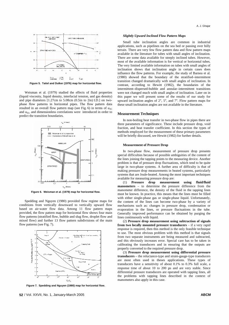
Figure 5. Taitel and Dulker (1976) map for horizon tal flow.
Weisman et al. (1979) studied the effects of fluid properties
(liquid viscosity, liquid density, interfacial tension, and gas density) and pipe diameters [1.27cm to 5.08cm (0.5in to 2in) I.D.] on two-phase flow patterns in horizontal pipes. The flow pattern data resulted in an overall flow pattern map (see Fig. 6) in terms of uSG and uSL, and dimensionless correlations were introduced in order to predict the transition boundaries.
Figure 6. Weisman et al. (1979) map for horizontal flow.
Spedding and Nguyen (1980) provided flow regime maps for
conditions from vertically downward to vertically upward flow based on air-water flow data. Among 11 flow pattern maps provided, the flow pattern map for horizontal flow shows four main flow patterns (stratified flow, bubble and slug flow, droplet flow and mixed flow) and further 13 flow pattern subdivisions of the main flow patterns (see Fig. 7).
Figure 7. Spedding and Nguyen (1980) map for horiz ontal flow.
Slightly Upward Inclined Flow Pattern Maps
Small tube inclination angles are common in industrial applications, such as pipelines on the sea bed or passing over hilly terrain. There are very few flow pattern data and flow pattern maps available in the literature for tubes with small angles of inclination. There are some data available for steeply inclined tubes. However, most of the available information is for vertical or horizontal tubes. The very limited available information on tubes with small angles of inclination shows that inclination angle in certain cases does influence the flow patterns. For example, the study of Barnea et al. (1980) showed that the boundary of the stratified–intermittent transition changed dramatically with small angles of inclination. In contrast, according to Hewitt (1982), the boundaries of the intermittent–dispersed-bubble and annular–intermittent transitions were not changed much with small angles of inclination. Later on in this paper we will present some of the results of our study for upward inclination angles of 2°, 5°, and 7°. Flow pattern maps for these small inclination angles are not available in the literature.
Measurement Techniques
In non-boiling heat transfer in two-phase flow in pipes there are three parameters of significance. These include pressure drop, void fraction, and heat transfer coefficient. In this section the types of methods employed for the measurement of these primary parameters will be briefly discussed, see Hewitt (1982) for further details.
Measurement of Pressure Drop
In two-phase flow, measurement of pressure drop presents special difficulties because of possible ambiguities of the content of the lines joining the tapping points to the measuring device. Another problem is that of pressure drop fluctuations, which tend to be quite large in two-phase systems. A further area of difficulty is that of making pressure drop measurements in heated systems, particularly systems that are Joule-heated. Among the most important techniques available for measuring pressure drop are:
(1) Pressure drop measurement using fluid/fluid manometers – to determine the pressure difference from the manometer difference, the density of the fluid in the tapping lines must be known. In practice, this means that the lines must be filled with either single-phase gas or single-phase liquid. Unfortunately, the content of the lines can become two-phase by a variety of mechanisms such as: changes in pressure drop, condensation or evaporation in the lines, or pressure fluctuations in the tube. Generally improved performance can be obtained by purging the lines continuously with liquid.
(2) Pressure drop measurement using subtraction of signals from two locally mounted pressure transducers – if a very rapid response is required, then this method is the only feasible technique to use. The most obvious problem with this method is that signals from two separate instruments are being measured and subtracted, and this obviously increases error. Special care has to be taken in calibrating the transducers and in ensuring that the outputs are properly converted to the required pressure drop.
(3) Pressure drop measurement using differential pressure transducers – the reluctance-type and strain-gauge-type transducers are most often used in theses applications. These types of transducers have a sensitivity of about 0.1% to 0.3% full scale, a response time of about 10 to 200 µs and are very stable. Since differential pressure transducers are operated with tapping lines, all the problems with tapping lines described in the context of manometers also apply in this case.
Non-Boiling Heat Transfer in Gas-Liquid Flow in Pipes – a Tutorial
J. of the Braz. Soc. of Mech. Sci. & Eng. Copyright 2005 by ABCM January-March 2005, Vol. XXVII, No.1 / 53
Measurement of Void Fraction
In two-phase flow, void fraction measurement is important in the calculation of pressure gradients and is relevant to the calculation of the amount of liquid and gas present in a system. There are numerous methods that have been proposed for the measurement of void fractions. For practical purposes, there are four main types of void fraction measurement:
(1) Pipe-average measurements –the average void fraction is required over a full section of pipe. A convenient and practical method for obtaining pipe-average measurements is the use of quick-closing valves. In this method, valves (which can be quickly and simultaneously operated) are placed at the beginning and end of a section of pipe over which the void fraction is to be determined. At the appropriate moment, the valves are actuated and the liquid phase trapped in the pipe is drained and its volume measured. Since the pipe volume is known or can be estimated, the pipe-average void fraction can be found. The valves can be linked mechanically or they can be operated by hand. For high pressure systems, solenoid valves may be used.
(2) Cross-sectional average measurements – the average void fraction is sought over a given pipe cross section. This can be achieved by using traversable single-beam radiation absorption methods, multibeam radiation absorption techniques, or neutron-scattering techniques.
(3) Chordal-average void fraction measurements – the average void fraction is measured across the diameter of a pipe. This type of measurement is usually achieved by means of radiation absorption methods.
(4) Local void fraction measurements – in this case void fraction is measured at a particular position within the pipe using local optical or electrical void probes. Usually, this void fraction is a time average at a point.
Measurement of Heat Transfer Coefficient
The heat transfer coefficient (defined as the ratio of the heat flux from a surface to the difference between the surface temperature and a suitably defined fluid bulk temperature) is of great importance in two-phase flow systems. For non-boiling heat transfer in gas-liquid flow in pipes, the most accepted and practical method of heat transfer coefficient measurement is the use of direct electrical heating with external thermocouples. In this method, alternating or direct current is fed through low-resistance leads and current clamps to the test section, which, typically, is a stainless steel tube through which the current passes. The power generation in the tube is determined by the product of the measured current that passes through the tube and the voltage drop across the tube. The power may be distributed nominally uniform if the wall thickness is uniform, but nonuniform axial and circumferential flux distributions are possible through the use of variable wall thickness. Usually, the temperature is measured on the outside of the tube wall with a thermocouple; the thermocouple junction is electrically insulated from the tube wall, using an epoxy adhesive with high thermal conductivity and electrical resistivity. The local inside tube wall temperature and the local peripheral inside wall heat flux is then calculated from measurements of the outside wall temperature, the heat generation within the pipe wall, and the thermophysical properties of the pipe material (electrical resistivity and thermal conductivity). From the local inside wall temperature, the local peripheral inside wall heat flux, and the local bulk temperature, the local peripheral heat transfer coefficient can be calculated. An example of the application of this method is the finite-difference based interactive computer program developed by Ghajar and Zurigat (1991). A brief description of the finite-difference
formulation and the equations used in the program, and the program’s capabilities will be presented next.
Finite Difference Formulation
The numerical solution of the conduction equation with internal heat generation and variable thermal conductivity and electrical resistivity was based on the following assumptions (Ghajar and Zurigat, 1991):
1. Steady-state conditions exist. 2. Peripheral and radial wall conduction exists. 3. Axial conduction is negligible. 4. The electrical resistivity and thermal conductivity of the tube
wall are functions of temperature. Based on the above assumptions, the expressions for calculation
of the local inside wall temperatures, heat flux, and local and average peripheral heat transfer coefficients are presented next.
Calculation of the Local Inside Wall Temperature and the
Local Inside Wall Heat Flux
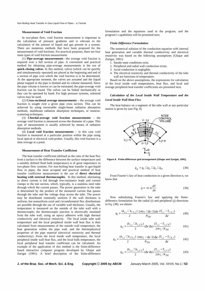
The heat balance on a segment of the tube wall at any particular station is given by (see Fig. 8)
Figure 8. Finite-difference grid arrangement (Ghaj ar and Zurigat, 1991).
4321 qqqqqg &&&&& +++= (38)
From Fourier’s law of heat conduction in a given direction n, we
know that
dn
dTAkq −=& (39)
Now substituting Fourier's law and applying the finite-
difference formulation for the radial (i) and peripheral (j) directions in Eq. (38), we obtain:
r
TT
N
zrrkkq jiji
TH
ijiji
∆−∆∆++
= −− )()2(2
2
)( ,1,,1,1
π& (40)
THi
jijijiji
Nr
TTzr
kkq
π2
)()(
2
)( 1,,1,,2
++ −∆∆
+=& (41)
r
TT
N
zrrkkq
jiji
TH
ijiji
∆−∆∆−+
= ++ )()2(2
2
)( ,1,,1,3
π& (42)
THi
jijijiji
Nr
TTzr
kkq
π2
)()(
2
)( 1,,1,,4
−− −∆∆
+=& (43)

A. J. Ghajar
/ Vol. XXVII, No. 1, January-March 2005 ABCM 54
The heat generated in the (i, j) elemental volume is given by:
RIqg2=& (44)
Substituting AlR /γ= and rNrA THi ∆= )/2( π into Eq. (44)
gives:
rNr
zIq
THig ∆
∆=
)2(2
πγ
& (45)
Substituting Eqs. (40) to (43) and (45) into Eq. (38) and solving
for Ti+1,j gives:
∆∆−
+
−∆
+−
−∆
+−
−∆
∆++−
∆
−= +
−−
++
−−
+TH
ijiji
jijii
THjiji
jijii
THjiji
jijiTH
ijiji
i
TH
jijiNr
rrkk
TTr
Nrkk
TTr
Nrkk
TTNr
rrkk
rr
NI
TT)2(
)(
)(4
)(
)(4
)(
)()2(
)(2
,1,
1,,1,,
1,,,1,
,1,,1,
2
,,1π
π
π
ππγ
(46) Equation (46) was used to calculate the temperature of the
interior nodes. In this equation, the thermal conductivity and electrical resistivity of each node's control volume were determined as a function of temperature from the following equations for 316 stainless steel (Ghajar and Zurigat, 1991).
Tk 0038.027.7 += (47)
T0213.067.27 +=γ (48)
where T is in °F, k is in Btu/hr-ft-°F, and γ is in µΩ-in. Once the local inside wall temperatures were calculated from Eq. (46), the local peripheral inside wall heat flux could be calculated from the heat balance equation [see Eq. (38)].
Calculation of the Local Peripheral and Local Average Heat
Transfer Coefficients
From the local inside wall temperature, the local peripheral inside wall heat flux and the local bulk fluid temperature, the local peripheral heat transfer coefficient could be calculated as follows:
)( BW TTqh −′′= & (49)
Note that, in this analysis, it was assumed that the bulk temperature increases linearly in the pipe from the inlet to the outlet according to the following equation:
LxTTTT INOUTINB )( −+= (50)
The local average heat transfer coefficient at each station is
calculated by the following equation:
( ) ( )[ ]kBkWkk TTqh −′′= & (51)
where k is the index of a thermocouple station.
Overall Mean Heat Transfer Coefficient
The local average peripheral values for inside wall temperature, inside wall heat flux, and heat transfer coefficient were then obtained by averaging all the appropriate individual local peripheral values at each axial location. The large variation in the circumferential wall temperature distribution, which is typical for two-phase gas-liquid flow in vertical, horizontal and slightly inclined tubes, leads to different heat transfer coefficients depending on which circumferential wall temperature was selected for calculations. In two-phase flow, in order to overcome the unbalanced circumferential heat transfer coefficient, Eq. (52) is recommended for calculation of the overall mean two-phase heat transfer coefficient, hTP.
∑=stN
kk
stTP h
Nh
1 (52)
where Nst is the number of all thermocouple stations and k is the index of a thermocouple station.
Physical Properties of the Working Fluids
The computer program developed by Ghajar and Zurigat (1991) also calculates the pertinent fluid flow and heat transfer dimensionless numbers. For this purpose the physical properties of the working fluids are needed. For example, for non-boiling two-phase heat transfer in air-water flow in pipes, the physical property correlations provided in Table 1 are recommended. Physical property expressions for other working fluids can easily be incorporated into the computer program.
Table 1. Physical properties of air and water, Vij ay (1978).
Fluid Equation for the Physical Property (T = Temperature in °F except where noted)
Range of Validity & Accuracy
Air
ρ (lbm/ft3) = p/RT where p is in lbf/ft
2, T is in °R, and R = 53.34 ft⋅lbf/lbm⋅°R cp (Btu/lbm⋅°F) = 7.540×10⁻⁶T + 0.2401 µ (lbm/ft⋅hr) = -2.637×10⁻⁸T 2 + 6.819×10⁻⁵T + 0.03936 k (Btu/hr⋅ft⋅°F) = -6.154×10⁻⁹T 2 + 2.591×10⁵T+ 0.01313
p ≤150 psi -10 ≤ T ≤ 242, 0.2 % -10 ≤ T ≤ 242, 0.1 % -10 ≤ T ≤ 242, 0.2 %
Water
ρ (lbm/ft3) = (2.101×10⁻⁸T 2 – 1.303×10⁻⁶T + 0.01602)-1
cp (Btu/lbm⋅°F) = 1.337×10⁻⁶T 2 – 3.374×10⁻⁴T + 1.018 µ (lbm/ft⋅hr) = (1.207×10⁻⁵T 2 + 3.863×10⁻³T + 0.0946)-1
k (Btu/hr⋅ft⋅°F) = 4.722×10⁻⁴T+ 0.3149
32 ≤ T ≤ 212, 0.1 % 32 ≤ T ≤ 212, 0.3 % 32 ≤ T ≤ 212, 1.0 % 32 ≤ T ≤ 212, 0.2 %

Non-Boiling Heat Transfer in Gas-Liquid Flow in Pipes – a Tutorial
J. of the Braz. Soc. of Mech. Sci. & Eng. Copyright 2005 by ABCM January-March 2005, Vol. XXVII, No.1 / 55
Data Reduction
The computer program developed by Ghajar and Zurigat’s (1991) can also be used to reduce the experimental data obtained for non-boiling two-phase heat transfer in gas-liquid flow in pipes under uniform wall heat flux boundary conditions. As will be discussed in the next section, at Oklahoma State University’s Heat Transfer Laboratory, we have used this computer program to reduce our air-water non-boiling heat transfer experimental data. The data reduction portion of the program reads a raw data file for a test run and then proceeds to perform all the required calculations. The results of the data reduction are saved in an output file for that particular test run. Figure 9 shows the data reduction results for the
case of air-water slug flow in a uniformly heated horizontal pipe. As can be seen from Fig. 9, the output file has four distinct sections to it. The first part of the output provides a detailed summary of the specifics of a test run, the second part gives the details of the pertinent heat transfer and flow information at each thermocouple station, the third part provides additional details at each thermocouple station that is more suited for the development of heat transfer correlations, and finally the forth and the last part of the output gives information about the flow parameters that are typically used in determination of flow patterns through established flow maps.
=============================================== RUN NUMBER 4649 FLOW PATTERN: S Air-Water Two-phase Heat Transfer Test Date: 01-04-2004 SI UNIT VERSION =============================================== LIQUID VOLUMETRIC FLOW RATE : 1.351 [m^3/hr] GAS VOLUMETRIC FLOW RATE : 3.086 [m^3/hr] LIQUID MASS FLOW RATE : 1351.36 [kg/hr] GAS MASS FLOW RATE : 4.777 [kg/hr] LIQUID V_SL : 0.615 [m/s] GAS V_SG : 1.406 [m/s] ROOM TEMPERATURE : 14.48 [C] INLET TEMPERATURE : 13.36 [C] OUTLET TEMPERATURE : 14.32 [C] AVG REFERENCE GAGE PRESSURE : 26169.74 [Pa] AVG LIQUID RE_SL : 14670 AVG GAS RE_SG : 3399 AVG LIQUID PR : 8.302 AVG GAS PR : 0.712 AVG LIQUID DENSITY : 1000.3 [kg/m^3] AVG GAS DENSITY : 1.548 [kg/m^3] AVG LIQUID SPECIFIC HEAT : 4.200 [kJ/kg-K] AVG GAS SPECIFIC HEAT : 1.007 [kJ/kg-K] AVG LIQUID VISCOSITY : 116.92e-05 [Pa-s] AVG GAS VISCOSITY : 17.84e-06 [Pa-s] AVG LIQUID CONDUCTIVITY : 0.592 [W/m-K] AVG GAS CONDUCTIVITY : 25.24e-03 [W/m-K] CURRENT TO TUBE : 460.51 [A] VOLTAGE DROP IN TUBE : 3.56 [V] AVG HEAT FLUX : 7089.12 [W/m^2] Q = AMP*VOLT : 1639.27 [W] Q = M*C*(T2 -T1) : 1512.20 [W] HEAT BALANCE ERROR : 7.75 [%] OUTSIDE SURFACE TEMPERATURE OF TUBE [C] 1 2 3 4 5 6 7 8 9 10 1 16.39 16.94 17.01 17.13 17.19 17.40 17.46 17.70 17.60 17.85 2 16.06 16.22 16.48 16.61 16.88 17.06 17.19 17.16 17.39 17.45 3 15.70 15.90 16.00 16.12 16.38 16.35 16.59 16.49 16.58 16.61 4 16.04 16.37 16.32 16.70 16.82 17.04 17.23 17.23 17.28 17.40 INSIDE SURFACE TEMPERATURES [C] 1 2 3 4 5 6 7 8 9 10 1 15.70 16.26 16.33 16.45 16.51 16.72 16.77 17.02 16.92 17.17 2 15.37 15.53 15.79 15.92 16.20 16.38 16.51 16.47 16.70 16.76 3 15.01 15.20 15.30 15.42 15.68 15.65 15.89 15.79 15.88 15.90 4 15.35 15.68 15.63 16.01 16.13 16.35 16.54 16.54 16.59 16.71 SUPERFICIAL REYNOLDS NUMBER OF GAS AT THE INSIDE TUBE WALL 1 2 3 4 5 6 7 8 9 10 1 3382 3377 3376 3375 3375 3373 3372 3370 3371 3369 2 3385 3384 3381 3380 3378 3376 3375 3375 3373 3372 3 3388 3387 3386 3385 3382 3383 3380 3381 3380 3380 4 3385 3382 3383 3379 3378 3376 3374 3374 3374 3373 SUPERFICAL REYNOLDS NUMBER OF LIQUID AT THE INSIDE TUBE WALL 1 2 3 4 5 6 7 8 9 10 1 15406 15625 15655 15703 15725 15810 15832 15930 15890 15991 2 15274 15337 15441 15492 15601 15673 15725 15712 15803 15826 3 15130 15206 15245 15292 15397 15383 15480 15440 15474 15485 4 15265 15396 15376 15527 15574 15663 15739 15738 15759 15806 INSIDE SURFACE HEAT FLUXES [W/m^2] 1 2 3 4 5 6 7 8 9 10 1 6639 6598 6603 6623 6645 6644 6661 6623 6658 6635 2 6686 6719 6695 6695 6681 6669 6674 6688 6656 6669 3 6739 6750 6752 6772 6764 6799 6788 6801 6808 6818 4 6689 6697 6718 6683 6691 6673 6668 6679 6672 6676 PERIPHERAL HEAT TRANSFER COEFFICIENT [W/m^2-K] 1 2 3 4 5 6 7 8 9 10 1 2911 2408 2424 2409 2448 2346 2383 2246 2415 2276 2 3433 3334 3064 3014 2780 2677 2639 2781 2622 2662 3 4251 4005 3990 3943 3577 3857 3547 3951 3967 4130 4 3471 3094 3325 2895 2865 2705 2599 2705 2746 2721
Figure 9. Date reduction program’s output file for a test run.

A. J. Ghajar
/ Vol. XXVII, No. 1, January-March 2005 ABCM 56
=============================================== RUN NUMBER 4649 continued FLOW PATTERN: S =============================================== ST MU_L[E-5 Pa-s] MU_G[E-6 Pa-s] CP[kJ/kg-K] K[W/m-K] RHO[kg/m^3] Bulk Wall Bulk Wall Lqd Gas Lqd Gas(E-3) Lqd Gas 1 118.23 112.34 17.82 17.91 4.200 1.007 0.591 25.21 1000.3 1.550 2 117.94 111.45 17.82 17.93 4.200 1.007 0.591 25.22 1000.3 1.550 3 117.65 111.17 17.83 17.93 4.200 1.007 0.591 25.22 1000.3 1.549 4 117.36 110.64 17.83 17.94 4.200 1.007 0.591 25.23 1000.3 1.549 5 117.07 110.14 17.84 17.95 4.200 1.007 0.591 25.24 1000.3 1.548 6 116.78 109.73 17.84 17.96 4.200 1.007 0.592 25.25 1000.3 1.548 7 116.49 109.30 17.85 17.96 4.200 1.007 0.592 25.25 1000.3 1.547 8 116.21 109.22 17.85 17.97 4.200 1.007 0.592 25.26 1000.3 1.547 9 115.93 109.04 17.85 17.97 4.199 1.007 0.592 25.27 1000.2 1.546 10 115.64 108.72 17.86 17.97 4.199 1.007 0.592 25.27 1000.2 1.546 ST X/D RESL RESG PRL PRG MUB/W(L) MUB/W(G) HT/HB HFLUX TB[C] TW[C] HCOEFF NU_L 1 6.38 14508 3403 8.40 0.712 1.052 0.995 0.685 6688 13.42 15.36 3456.3 162.98 2 15.50 14544 3402 8.38 0.712 1.058 0.994 0.601 6691 13.52 15.67 3110.4 146.64 3 24.61 14580 3401 8.36 0.712 1.058 0.994 0.608 6692 13.61 15.76 3104.9 146.34 4 33.73 14616 3400 8.34 0.712 1.061 0.994 0.611 6693 13.70 15.95 2976.0 140.23 5 42.84 14652 3400 8.31 0.712 1.063 0.994 0.684 6695 13.79 16.13 2866.4 135.04 6 51.96 14688 3399 8.29 0.712 1.064 0.994 0.608 6696 13.89 16.27 2803.9 132.06 7 61.08 14724 3398 8.27 0.712 1.066 0.993 0.672 6698 13.98 16.43 2732.8 128.69 8 70.19 14760 3397 8.25 0.712 1.064 0.994 0.569 6698 14.07 16.46 2807.1 132.16 9 79.31 14797 3396 8.22 0.712 1.063 0.994 0.609 6699 14.16 16.52 2838.1 133.58 10 88.42 14833 3395 8.20 0.712 1.064 0.994 0.551 6700 14.25 16.63 2813.5 132.39 =============================================== RUN NUMBER 4649 continued FLOW PATTERN: S QUANTITIES OF MAIN PARAMETERS =============================================== INCLINATION ANGLE : 2.000 [DEG] TOTAL MASS FLUX(Gt): 617.775 [kg/m^2-s] QUALITY(x) : 0.004 SLIP RATIO(K) : 1.809 VOID FRACTION(alpa): 0.558 V_SL : 0.615 [m/s] V_SG : 1.406 [m/s] RE_SL : 14670 RE_SG : 3399 RE_TP : 18069 X(Taitel & Dukler) : 9.614 T(Taitel & Dukler) : 0.137 Y(Taitel & Dukler) : 172.059 F(Taitel & Dukler) : 0.106 K(Taitel & Dukler) : 12.828 X (Breber) : 9.614 j*g(Breber) : 0.106
Figure 9. (Continued).
Oklahoma State University’s Heat Transfer Laboratory Research in Two-Phase Flow
In the next several sections we present the results of our extensive literature search, a detailed development of our proposed heat transfer correlation and its application to experimental data in vertical and horizontal pipes, a detailed description of our experimental setup, our flow visualization results for different flow patterns, our experimental results for slug and annular flows in horizontal and inclined tubes, our proposed heat transfer correlation for these flow patterns and pipe orientations, and finally our future plans.
Comparison of Non-Boiling Two-Phase Heat Transfer
Correlations with Experimental Data
Numerous heat transfer correlations and experimental data for non-boiling forced convective heat transfer during gas-liquid two-phase flow in vertical and horizontal pipes have been published over the past 50 years. In a study published by Kim et al. (1999), a comprehensive literature search was carried out and a total of 38 two-phase flow heat transfer correlations were identified. The validity of these correlations and their ranges of applicability have been documented by the original authors. In most cases, the identified heat transfer correlations were based on a small set of experimental data with a limited range of variables and liquid-gas
combinations. In order to assess the validity of those correlations, they were compared against seven extensive sets of two-phase flow non-boiling heat transfer experimental data available from the literature, for vertical and horizontal tubes and different flow patterns and fluids. For consistency, the validity of the identified heat transfer correlations were based on the comparison between the predicted and experimental two-phase heat transfer coefficients meeting the ±30% criterion. A total of 524 data points from the five available experimental studies (see Table 2) were used for these comparisons. The experimental data included five different liquid-gas combinations (water-air, glycerin-air, silicone-air, water-helium, water-Freon 12), and covered a wide range of variables, including liquid and gas flow rates and properties, flow patterns, pipe sizes, and pipe inclination. Five of these experimental data sets are concerned with a wide variety of flow patterns in vertical pipes and the other two data sets are for limited flow patterns (slug and annular) within horizontal pipes.
Tables 3 and 4 show 20 of the 38 heat transfer correlations that were identified in the study of Kim et al. (1999). The rest of the two-phase flow heat transfer correlations were not tested, since the required information for the correlations was not available through the identified experimental studies. In assessing the ability of the 20 identified heat transfer correlations, their predictions were compared with the seven sets of experimental data, both with and without considering the restrictions on ReSL and uSG/uSL accompanying the correlations.
Non-Boiling Heat Transfer in Gas-Liquid Flow in Pipes – a Tutorial
J. of the Braz. Soc. of Mech. Sci. & Eng. Copyright 2005 by ABCM January-March 2005, Vol. XXVII, No.1 / 57
Table 2. Ranges of the experimental data used in t he study of Kim et al. (1999).
Water-Air Vertical
Data (139 Points) of Vijay (1978)
16.71 ≤ Lm& (lbm/hr) ≤ 8996
0.058 ≤ Gm& (lbm/hr) ≤ 216.82
0.007 ≤ XTT ≤ 433.04 0.061 ≤ ∆pTP (psi) ≤ 17.048
5.503 ≤ PrL ≤ 6.982 101.5 ≤ hTP (Btu/hr⋅ft2⋅°F) ≤ 7042.3
0.06 ≤ uSL(ft/sec) ≤ 34.80 0.164 ≤ uSG(ft/sec) ≤ 460.202
59.64 ≤ Tm (°F) ≤ 83.94 0.007 ≤ ∆pTPF (psi) ≤ 16.74
0.708 ≤ PrG ≤ 0.710 0.813 ≤ µW/µB ≤ 0.933
231.83 ≤ ReSL ≤ 126630 43.42 ≤ ReSG ≤ 163020 14.62 ≤ pm (psi) ≤ 74.44
0.033 ≤ α ≤ 0.997 11.03 ≤ NuTP ≤ 776.12
L/D = 52.1, D = 0.46 in.
Glycerin-Air Vertical
Data (57 Points) of Vijay (1978)
100.5 ≤ Lm& (lbm/hr) ≤ 1242.5
0.085 ≤ Gm& (lbm/hr) ≤ 99.302
0.15 ≤ XTT ≤ 407.905 1.317 ≤ ∆pTP (psi) ≤ 20.022 6307.04 ≤ PrL ≤ 6962.605
54.84 ≤ hTP (Btu/hr⋅ft2⋅°F) ≤ 159.91
0.31 ≤ uSL (ft/sec) ≤ 3.80 0.217 ≤ uSL (ft/sec) ≤ 117.303
80.40 ≤ Tm (°F) ≤ 82.59 1.07 ≤ ∆pTPF (psi) ≤ 19.771
0.708 ≤ PrG ≤ 0.709 0.513 ≤ µW/µB ≤ 0.610
1.77 ≤ ReSL ≤ 21.16 63.22 ≤ ReSG ≤ 73698
17.08 ≤ pm (psi) ≤ 62.47 0.0521 ≤ α ≤ 0.9648 12.78 ≤ NuTP ≤ 37.26
L/D = 52.1, D = 0.46 in.
Silicone-Air Vertical
Data (162 points) of Rezkallah (1987)
17.3 ≤ Lm& (lbm/hr) ≤ 196
0.07 ≤ Gm& (lbm/hr) ≤ 157.26
72.46 ≤ TW (°F) ≤113.90 0.037 ≤ ∆pTP (psi) ≤ 9.767
61.0 ≤ PrL ≤ 76.5 29.9 ≤ hTP (Btu/hr⋅ft2⋅°F) ≤ 683.0
0.072 ≤ uSL (ft/sec) ≤ 30.20 0.17 ≤ uSL (ft/sec) ≤ 363.63
66.09 ≤ TB (°F) ≤ 89.0 0.094 ≤ ∆pTPF (psi) ≤ 9.074
0.079 ≤ PrG ≤ 0.710
47.0 ≤ ReSL ≤ 20930 52.1 ≤ ReSG ≤ 118160 13.9 ≤ pm (psi) ≤ 45.3
0.011 ≤ α ≤ 0.996 17.3 ≤ NuTP ≤ 386.8
L/D = 52.1, D = 0.46 in.
Water-Helium Vertical
Data (53 Points) of Aggour (1978)
267 ≤ Lm& (lbm/hr) ≤ 8996
0.020 ≤ Gm& (lbm/hr) ≤ 33.7
0.16 ≤ XTT ≤ 769.6 0.3 ≤ ∆pTP (psi) ≤ 13.2
5.78 ≤ PrL ≤ 7.04 794 ≤ hTP (Btu/hr⋅ft2⋅°F) ≤ 6061
1.03 ≤ uSL (ft/sec) ≤ 34.70 0.423 ≤ uSL (ft/sec) ≤ 483.6
67.4 ≤ Tm (°F) ≤ 82.0 0.01 ≤ ∆pTPF (psi) ≤ 12.5
0.6908 ≤ PrG ≤ 0.691 83.9 ≤ TW (°F) ≤ 95.7
3841 ≤ ReSL ≤ 125840 14.0 ≤ ReSG ≤ 23159 15.5 ≤ pm (psi) ≤ 53.3
0.038 ≤ α ≤ 0.958 86.6 ≤ NuTP ≤ 668.2
L/D = 52.1, D = 0.46 in
Water-Freon 12 Vertical
Data (44 Points) of Aggour (1978)
267 ≤ Lm& (lbm/hr) ≤ 3598
0.84 ≤ Gm& (lbm/hr) ≤ 206.59
0.16 ≤ XTT ≤ 226.5 0.04 ≤ ∆pTP (psi) ≤ 4.92
5.63 ≤ PrL ≤ 6.29 800 ≤ hTP (Btu/hr⋅ft2⋅°F) ≤ 4344
1.03 ≤ uSL (ft/sec) ≤ 13.89 0.51 ≤ uSL (ft/sec) ≤ 117.7 75.26 ≤ TMIX (°F) ≤ 83.89 0.02 ≤ ∆pTPF (psi) ≤ 4.48
0.769 ≤ PrG ≤ 0.77 90.36 ≤ TW (°F) ≤ 94.89
4190 ≤ ReSL ≤ 51556 859.5 ≤ ReSG ≤ 209430 15.8 ≤ pm (psi) ≤ 27.8
0.035 ≤ α ≤ 0.934 87.1 ≤ NuTP ≤ 472.4
L/D = 52.1, D = 0.46 in
Water-Air Horizontal
Data (48 points) of Pletcher (1966)
0.069 ≤ Lm& (lbm/sec) ≤ 0.3876
0.22 ≤ ∆pa/L (lbf/ft3) ≤ 26.35 7.23 ≤ φL ≤ 68.0
7372 ≤ q'' (Btu/hr⋅ft2) ≤ 11077
0.03 ≤ Gm& (lbm/sec) ≤ 0.2568
0.021 ≤ XTT ≤ 0.490 73.6 ≤ TW (°F) ≤ 107.1
433 ≤ hTP (Btu/hr⋅ft2⋅°F) ≤ 1043.8
7.84 ≤ ∆p/L (lbf/ft3) ≤ 137.5 1.45 ≤ φG ≤ 3.54
64.9 ≤ Tm (°F) ≤ 99.4 L/D = 60.0, D = 1.0 in.
Water-Air Horizontal
Data (21 points) of King (1952)
1375 ≤ Lm& (lbm/hr) ≤ 6410
1570 ≤ ReSG ≤ 84200 136.8 ≤ Tm (°F) ≤ 144.85
1.027 ≤ ∆pTP (psi) ≤ 22.403 1.35 ≤ hTP / hL ≤ 3.34
0.82 ≤ Gm& (SCFM) ≤ 43.7
0.41 ≤ XTT ≤ 29.10 184.3 ≤ TW (°F) ≤ 211.3
1462 ≤ hTP (Btu/hr⋅ft2⋅°F) ≤ 4415 1.35 ≤ φL ≤ 8.20
22500 ≤ ReSL ≤ 119000 0.117 ≤ RL ≤ 0.746
15.8 ≤ pm (psi) ≤ 55.0 0.33 ≤ uSG/uSL ≤ 7.65
L/D =252, D = 0.737 in.
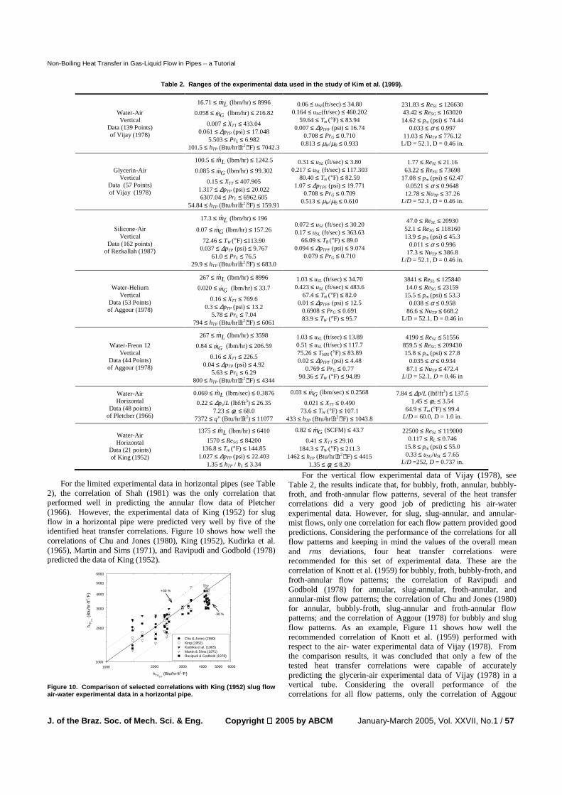
For the limited experimental data in horizontal pipes (see Table
2), the correlation of Shah (1981) was the only correlation that performed well in predicting the annular flow data of Pletcher (1966). However, the experimental data of King (1952) for slug flow in a horizontal pipe were predicted very well by five of the identified heat transfer correlations. Figure 10 shows how well the correlations of Chu and Jones (1980), King (1952), Kudirka et al. (1965), Martin and Sims (1971), and Ravipudi and Godbold (1978) predicted the data of King (1952).
10001000
Chu & Jones (1980)King (1952)Kudirka et al. (1965)Martin & Sims (1971)Ravipudi & Godbold (1978)
2000 3000 4000 5000 6000
2000
3000
4000
5000
6000
+30 %
-30 %
h TP
CA
L (B
tu/h
r-ft2 -°F
)
hTPEXP (Btu/hr-ft2-°F)
Figure 10. Comparison of selected correlations wit h King (1952) slug flow air-water experimental data in a horizontal pipe.
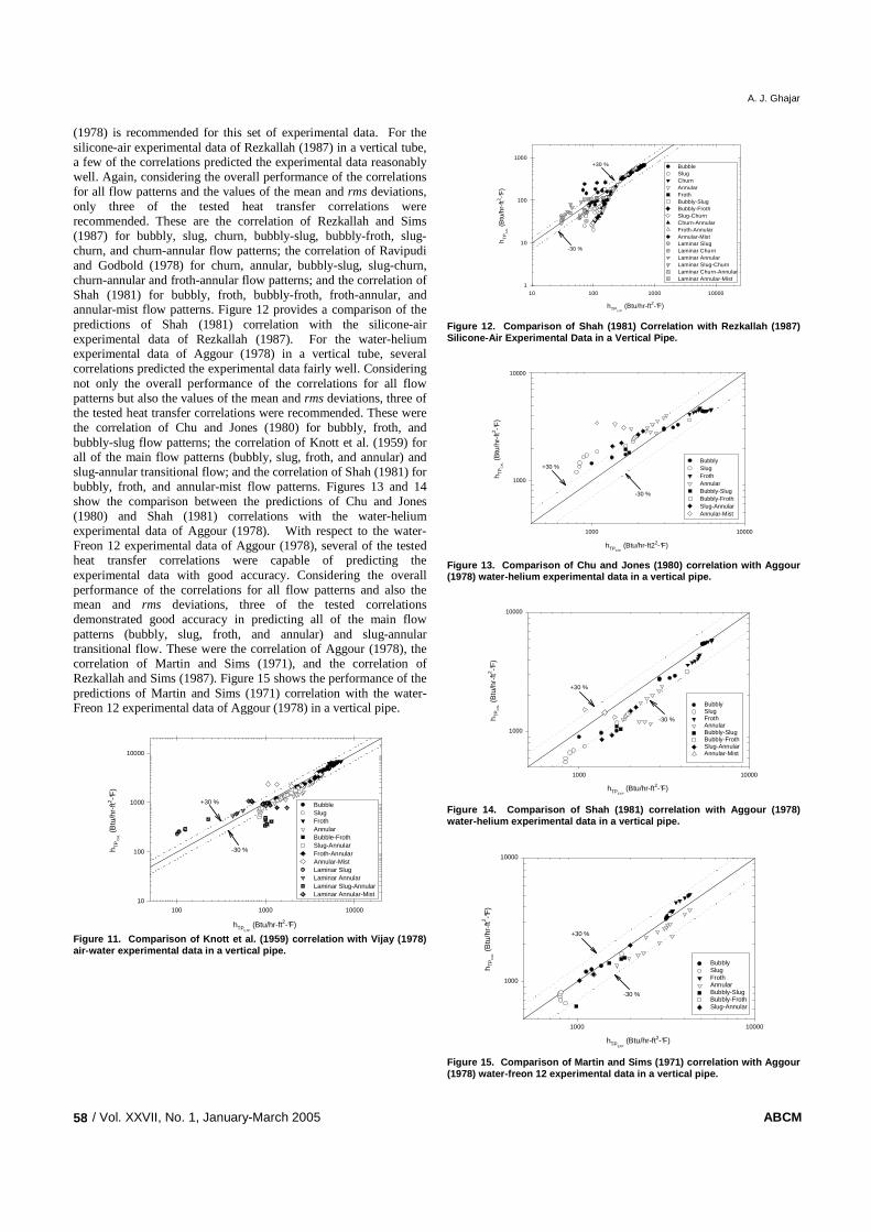
For the vertical flow experimental data of Vijay (1978), see Table 2, the results indicate that, for bubbly, froth, annular, bubbly-froth, and froth-annular flow patterns, several of the heat transfer correlations did a very good job of predicting his air-water experimental data. However, for slug, slug-annular, and annular-mist flows, only one correlation for each flow pattern provided good predictions. Considering the performance of the correlations for all flow patterns and keeping in mind the values of the overall mean and rms deviations, four heat transfer correlations were recommended for this set of experimental data. These are the correlation of Knott et al. (1959) for bubbly, froth, bubbly-froth, and froth-annular flow patterns; the correlation of Ravipudi and Godbold (1978) for annular, slug-annular, froth-annular, and annular-mist flow patterns; the correlation of Chu and Jones (1980) for annular, bubbly-froth, slug-annular and froth-annular flow patterns; and the correlation of Aggour (1978) for bubbly and slug flow patterns. As an example, Figure 11 shows how well the recommended correlation of Knott et al. (1959) performed with respect to the air- water experimental data of Vijay (1978). From the comparison results, it was concluded that only a few of the tested heat transfer correlations were capable of accurately predicting the glycerin-air experimental data of Vijay (1978) in a vertical tube. Considering the overall performance of the correlations for all flow patterns, only the correlation of Aggour
A. J. Ghajar
/ Vol. XXVII, No. 1, January-March 2005 ABCM 58
(1978) is recommended for this set of experimental data. For the silicone-air experimental data of Rezkallah (1987) in a vertical tube, a few of the correlations predicted the experimental data reasonably well. Again, considering the overall performance of the correlations for all flow patterns and the values of the mean and rms deviations, only three of the tested heat transfer correlations were recommended. These are the correlation of Rezkallah and Sims (1987) for bubbly, slug, churn, bubbly-slug, bubbly-froth, slug-churn, and churn-annular flow patterns; the correlation of Ravipudi and Godbold (1978) for churn, annular, bubbly-slug, slug-churn, churn-annular and froth-annular flow patterns; and the correlation of Shah (1981) for bubbly, froth, bubbly-froth, froth-annular, and annular-mist flow patterns. Figure 12 provides a comparison of the predictions of Shah (1981) correlation with the silicone-air experimental data of Rezkallah (1987). For the water-helium experimental data of Aggour (1978) in a vertical tube, several correlations predicted the experimental data fairly well. Considering not only the overall performance of the correlations for all flow patterns but also the values of the mean and rms deviations, three of the tested heat transfer correlations were recommended. These were the correlation of Chu and Jones (1980) for bubbly, froth, and bubbly-slug flow patterns; the correlation of Knott et al. (1959) for all of the main flow patterns (bubbly, slug, froth, and annular) and slug-annular transitional flow; and the correlation of Shah (1981) for bubbly, froth, and annular-mist flow patterns. Figures 13 and 14 show the comparison between the predictions of Chu and Jones (1980) and Shah (1981) correlations with the water-helium experimental data of Aggour (1978). With respect to the water-Freon 12 experimental data of Aggour (1978), several of the tested heat transfer correlations were capable of predicting the experimental data with good accuracy. Considering the overall performance of the correlations for all flow patterns and also the mean and rms deviations, three of the tested correlations demonstrated good accuracy in predicting all of the main flow patterns (bubbly, slug, froth, and annular) and slug-annular transitional flow. These were the correlation of Aggour (1978), the correlation of Martin and Sims (1971), and the correlation of Rezkallah and Sims (1987). Figure 15 shows the performance of the predictions of Martin and Sims (1971) correlation with the water-Freon 12 experimental data of Aggour (1978) in a vertical pipe.
hTPEXP (Btu/hr-ft2-°F)
100 1000 10000
h TP
CA
L (B
tu/h
r-ft2 -°F
)
10
100
1000
10000
BubbleSlugFrothAnnularBubble-FrothSlug-AnnularFroth-AnnularAnnular-MistLaminar SlugLaminar AnnularLaminar Slug-AnnularLaminar Annular-Mist
+30 %
-30 %
Figure 11. Comparison of Knott et al. (1959) corre lation with Vijay (1978) air-water experimental data in a vertical pipe.
hTPEXP (Btu/hr-ft2-°F)
10 100 1000 10000
h TP
CA
L (B
tu/h
r-ft2 -°F
)
1
10
100
1000
BubbleSlugChurnAnnularFrothBubbly-SlugBubbly-FrothSlug-ChurnChurn-AnnularFroth-AnnularAnnular-MistLaminar SlugLaminar ChurnLaminar AnnularLaminar Slug-ChurnLaminar Churn-AnnularLaminar Annular-Mist
+30 %
-30 %
Figure 12. Comparison of Shah (1981) Correlation w ith Rezkallah (1987) Silicone-Air Experimental Data in a Vertical Pipe.
hTPEXP (Btu/hr-ft22-°F)
1000 10000
h TP
CA
L (
Btu
/hr-
ft2 -°F)
1000
10000
BubblySlugFrothAnnularBubbly-SlugBubbly-FrothSlug-AnnularAnnular-Mist
-30 %
+30 %
Figure 13. Comparison of Chu and Jones (1980) corr elation with Aggour (1978) water-helium experimental data in a vertical pipe.
hTPEXP (Btu/hr-ft2-°F)
1000 10000
h TP
CA
L (B
tu/h
r-ft2 -°F
)
1000
10000
BubblySlugFrothAnnularBubbly-SlugBubbly-FrothSlug-AnnularAnnular-Mist
-30 %
+30 %
Figure 14. Comparison of Shah (1981) correlation w ith Aggour (1978) water-helium experimental data in a vertical pipe.
hTPEXP (Btu/hr-ft2-°F)
1000 10000
h TP
CA
L (B
tu/h
r-ft2
-°F)
1000
10000
BubblySlugFrothAnnularBubbly-SlugBubbly-FrothSlug-Annular
-30 %
+30 %
Figure 15. Comparison of Martin and Sims (1971) co rrelation with Aggour (1978) water-freon 12 experimental data in a vertic al pipe.

Non-Boiling Heat Transfer in Gas-Liquid Flow in Pipes – a Tutorial
J. of the Braz. Soc. of Mech. Sci. & Eng. Copyright 2005 by ABCM January-March 2005, Vol. XXVII, No.1 / 59
The results comparing the twenty identified non-boiling heat transfer correlations (see Table 3) and the seven sets of experimental data (see Table 2) are summarized in Table 5 for major flow patterns in vertical and horizontal pipes and Table 6 for transitional flow patterns in vertical pipes. The shaded cells of Tables 5 and 6 indicate the correlations that best satisfied the ±30% two-phase heat transfer coefficient criterion that was set. There were no remarkable differences for the recommendations of the heat transfer correlations based on the results with and without the restrictions on ReSL and uSG/uSL, except for the correlations of Chu and Jones (1980) and Ravipudi and Godbold (1978), as applied to the air-water experimental data of Vijay (1978). Based on the results without the authors' restrictions, the correlation of Chu and Jones (1980) was recommended for only annular, bubbly-froth, slug-annular, and froth-annular flow patterns; and the correlation of Ravipudi and
Godbold (1978) was recommended for only annular, slug-annular, and froth-annular flow patterns of the vertical tube water-air experimental data. However, considering the ReSL and uSG/uSL, restrictions, the correlation of Chu and Jones (1980) was recommended for all vertical tube air-water flow patterns including transitional flow patterns except the annular-mist flow pattern; and the correlation of Ravipudi and Godbold (1978) was recommended for slug, froth, and annular flow patterns and for all of the transitional flow patterns of the vertical water-air experimental data of Vijay (1978). With regard to air-water flow in horizontal pipes, Kim et al. (1999) recommended use of Shah (1981) correlation for annular flow, and use of the Chu and Jones (1980), Kudirka et al. (1965), and Ravipudi and Godbold (1978) correlations for slug flow (see Table 5).
Table 3. Heat Transfer Correlations Chosen for the Study of Kim et al. (1999).
Source Heat Transfer Correlations Source Heat Transfer Correlations
Aggour (1978)
31)1( −−= αLTP hh Laminar (L) 14.031 )()Pr(615.1 WBLSLL LDReNu µµ= (L)
83.0)1( −−= αLTP hh Turbulent (T)
( ) 33.05.083.00155.0 WBLSLL PrReNu µµ= (T)
Knott et al. (1959)
31
1
+=
SL
SG
L
TPu
u
h
h
where hL is from Sieder & Tate (1936)
Chu & Jones (1980)
( ) ( ) 17.014.03155.043.0 ppPrReNu AWBLTPTP µµ= Kudirka et al. (1965) ( ) ( ) ( ) 14.031416.081125 WBLSLLGSLSGTP PrReuuNu µµµµ=
Davis & David (1964)
4.087.028.0
060.0 LLG
LTP Pr
DGxNu
=
µρρ Martin & Sims
(1971) SLSGLTP uuhh 64.01+=
where hL is from Sieder & Tate (1936)
Dorresteijn (1970)
31)1( −−= αLTP hh (L) 8.0)1( −−= αLTP hh (T)
( ) 14.033.09.00123.0 WBLSLL PrReNu µµ=
Oliver & Wright (1964)
( )LLLTP RRNuNu 2.02.1 36.0 −=
0.141/3
L )/(/ D)+(
615.1 WBLG
L LDPrA
QQNu µµ
µρ
=
Dusseau (1968)
4.087.00.029 = LTPTP PrReNu Ravipudi & Godbold (1978) ( ) ( ) ( ) 14.0316.02.03.056.0 WBLSLLGSLSGTP PrReuuNu µµµµ=
Elamvaluthi &
Srinivas (1984)
14.0317.0
41
5.0
=
W
BLTP
L
GTP PrReNu
µµ
µµ Rezkallah &
Sims (1987)
9.0)1( −−= αLTP hh
where hL is from Sieder & Tate (1936)
Groothuis & Hendal
(1959)
14.03187.0 )()(0.029 = WBLTPTP PrReNu µµ
(for water-air) 14.03139.0 )(Pr 2.6 = WBLLTPTP ReNu µµ
(for (gas-oil)-air)
Serizawa et al. (1975)
27.14621 −+= TTLTP Xhh where hL is from Sieder & Tate (1936)
Hughmark (1965) ( )
14.03121 75.1
= −
W
B
LL
LLLTP
LkR
cmRNu
µµ& Shah (1981)
( ) 1 41SLSGLTP uuhh +=
0.141/3 )()PrRe(86.1 WBLSLLLDNu = (L)
( ) 14.04.08.0 Pr023.0 WBLSLL ReNu = (T)
Khoze et al. (1976)
4.055.02.026.0 LSLSGTP PrReReNu = Ueda & Hanaoka (1967)
[ ] )1(035.01075.0 6.0 −+= LLmTP PrPrReNu
King (1952)
32.0
5.0
52.0
025.01
∆∆
∆∆
+=
−
LTPSG
L
L
TPL
p
L
p
Re
R
h
h
4080023.0 .L
.SLL PrReNu =
Vijay et al. (1982)
451.0)/( LTPFLTP pphh ∆∆= 0.141/3 )()LPrRe( 615.1 WBLSLL DNu = (L)
0.335.0830 )(Re0155.0 WBL.
SLL PrNu = (T)
Sieder & Tate
(1936)
0.1431 )()(86.1 WBLSLL LD PrReNu = (L)
0.1433.08.0 )(027.0 WBLSLL PrReNu = (T)
Note: α and RL are taken from the original experimental data for this study. ReSL < 4000 implies laminar flow, otherwise turbulent; and for Shah (1981), replace 4000 by 170. With regard to the eqs. given for Shah (1981) above, the laminar two-phase correlation was used along with the appropriate single-phase correlation, since Shah (1981) recommended a graphical turbulent two-phase correlation.

A. J. Ghajar
/ Vol. XXVII, No. 1, January-March 2005 ABCM 60
Table 4. Limitations of the Heat Transfer Correlat ions Used in the Study of Kim et al. (1999) (See No menclature for Abbreviations).
Source Fluids L/D Orient. LG mm && / uSG/uSL ReSG ReSL PrL Flow Pattern(s)
Aggour (1978)
A-W, Helium-W, Freon12-W
52.1 V 7.5×10⁻⁵-5.72×10⁻² 0.02-470 13.95-2.95×10⁵ 5.78-7.04 B, S, A, B-S, B-
F, S-A, A-M
Chu & Jones (1980)
W-A 34 V 0.12-4.64 540-2700 16000-112000 B, S, F-A
Davis & David (1964)
Gas-Liquid H & V A, M-A
Dorresteijn (1970)
A-Oil 16 V 0.004-4500 300-66000 B, S, A
Dusseau (1968)
A-W 67 V 45-350 0-4.29×10⁴ 1.4×10⁴-4.9×10⁴
F
Elamvaluthi & Srinivas
(1984)
A-W A-Glycerin
86 V 0.3-2.5 0.6-4.6
300-14300 B, S
Groothuis & Hendal
(1959)
A-W Gas-Oil-A
14.3 V 244-977 269-513
1-250 0.6-80
>5000
1400-3500
Hughmark (1965)
Gas-Liquid H S
Khoze et al. (1976)
A-W, A-
Polymethylsiloxane A-Diphenyloxide
60-80 V 4000-37000 3.5-210 4.1-90 A
King (1952) A-W 252 H 0.327-7.648 1570-8.28×10⁴ 22500-
11.9×10⁴ S
Knott et al. (1959)
Petroleum oil-Nitrogen gas
119 V 1.57×10⁻³-1.19 0.1-4 6.7-162 126-3920 B
Kudirka et al. (1965)
A-W, A-Ethylene glycol
17.6 V 1.92×10⁻⁴-0.1427 0-0.11
0.16-75 0.25-67
5.5×10⁴-49.5×10⁴ 380-1700
140 @ 37.8°C
B, S, F
Martin & Sims (1971)
A-W 17 H B, S, A
Oliver & Wright (1964)
A-85% Glycol, A-1.5% SCMC, A-0.5% Polyox
H 500-1800 S
Ravipudi & Godbold (1978)
A-W, A-Toluene, A-Benzene, A-Methanol
V 1-90 3562-82532 8554-89626 F
Rezkallah & Sims (1987)
A, W, Oil, etc.; 13 Liquid-Gas combinations
52.1 V 0.01-7030 1.8-1.3×10⁵ 4.2-7000
B, S, C, A, F, B-S, B-F,
S-C, S-A, C-A, F-A
Serizawa et al. (1975)
A-W 35 V B
Shah (1981)
A, W, Oil, Nitrogen, Glycol, etc.;
10 combinations
H & V 0.004-4500 7-170 B, S, F, F-A, M
Ueda & Hanaoka (1967)
A-Liquid 67 V 9.4×10⁻⁴-0.059 4-50 4-160 S, A
Vijay et al. (1982)
A-W, A-Glycerin, Helium-W, Freon12-W
52.1 V 0.005-7670 1.8-130000 5.5-7000 B, S, F, A, M, B-F, S-A, F-A, A-
M

Non-Boiling Heat Transfer in Gas-Liquid Flow in Pipes – a Tutorial
J. of the Braz. Soc. of Mech. Sci. & Eng. Copyright 2005 by ABCM January-March 2005, Vol. XXVII, No.1 / 61
Table 5. Recommended correlations by Kim et al. (1 999) from the general comparisons with regard to pi pe orientation, fluids, and major flow patterns (see Nomenclature for abbreviations).
Vertical Pipe Horizontal Water-Air Glycerin-Air Silicone-Air Water-Helium Water-Freon 12 Water-Air
Correlations with Restrictions on ReSL and
uSG/uSL B S F A B S F A B S C A F B S F A B S F A A S Aggour (1978) -V -V -V -V -V -V -V -V -V -V
Chu & Jones (1980) RV RV RV RV R R RV V RV R RV RV Knott et al. (1959) V V V R V V V V V V
Kudirka et al. (1965) RV V RV Ravipudi & Godbold
(1978) RV RV RV V RV V R RV V RV RV
Rezkallah & Sims (1987) RV RV RV RV RV RV RV RV RV RV Shah (1981) V V RV V V V V V V V
Water-Air Glycerin-Air Silicone-Air Water-Helium Water-Freon 12 Water-Air Correlations with No Restrictions B S F A B S F A B S C A F B S F A B S F A A S
Aggour (1978) N N N N N N N N N N Chu & Jones (1980) N N N N N Knott et al. (1959) N N N N N N N N N
Kudirka et al. (1965) N Martin & Sims (1971) N N N N N N N Ravipudi & Godbold
(1978) N N N N N
Rezkallah & Sims (1987) N N N N N N N N N Shah (1981) N N N N N N N N N N
Water-Air Glycerin-Air Silicone-Air Water-Helium Water-Freon 12 Water-Air Correlation Recommendations Based on Comparisons Above B S F A B S F A B S C A F B S F A B S F A A S
Aggour (1978) √ √ √ √ √ √ √ √ √ √ Chu & Jones (1980) √ √ √ √ √ Knott et al. (1959) √ √ √ √ √ √ √
Kudirka et al. (1965) √ Martin & Sims (1971) √ √ √ √ √ √ √ Ravipudi & Godbold
(1978) √ √ √ √ √
Rezkallah & Sims (1987) √ √ √ √ √ √ √ √ √ Shah (1981) √ √ √ √ √ √ √ √ √ √
Note: R = Recommended correlation with the range of ReSL. V = Recommended correlation with the range of uSG/uSL. N = Recommended correlation with no restrictions. √ = Recommended correlation with and without restrictions. - = Correlation that did not provide ranges for either ReSL or uSG/uSL. Correlation of Martin & Sims (1971) did not provide ranges for ReSL and uSG/uSL.

A. J. Ghajar
/ Vol. XXVII, No. 1, January-March 2005 ABCM 62
Table 6. Recommended correlations by Kim et al. (1 999) from the general comparisons with regard to ex perimental fluids and transition flow patterns (see Nomenclature for abbreviations).
Vertical Pipe
Water-Air Glycerin-
Air Silicone-Air Water-Helium
Water-Freon 12
Correlations with Restrictions on ReSL and
uSG/uSL B-F
S-A
F-A
A-M
B-S S-A B-S
B-F
S-C
C-A
F-A
A-M
B-S
B-F
S-A
A-M
B-S
B-F
S-A
Aggour (1978) -V -V -V Chu & Jones (1980) RV RV RV R V V Knott et al. (1959) V V V
Kudirka et al. (1965) RV R V RV RV Ravipudi & Godbold
(1978) RV RV RV RV V V V RV R R V
Rezkallah & Sims (1987)
RV RV RV RV RV RV RV RV
Shah (1981) V V V V R V
Water-Air Glycerin-
Air Silicone-Air Water-Helium
Water-Freon 12 Correlations with No
Restrictions B-F
S-A
F-A
A-M
B-S S-A B-S
B-F
S-C
C-A
F-A
A-M
B-S
B-F
S-A
A-M
B-S
B-F
S-A
Aggour (1978) N N N N N Chu & Jones (1980) N N N N N Knott et al. (1959) N N N N N
Kudirka et al. (1965) N N N Martin & Sims (1971) N N N Ravipudi & Godbold
(1978) N N N N N N N N N
Rezkallah & Sims (1987)
N N N N N N N N
Shah (1981) N N N N N N N
Water-Air Glycerin-
Air Silicone-Air Water-Helium
Water-Freon 12
Correlation Recommendations
Based on Comparisons Above
B-F
S-A
F-A
A-M
B-S S-A B-S
B-F
S-C
C-A
F-A
A-M
B-S
B-F
S-A
A-M
B-S
B-F
S-A
Aggour (1978) √ √ √ Chu & Jones (1980) √ √ √ √ √ Knott et al. (1959) √ √ √
Kudirka et al. (1965) √ √ √ Martin & Sims (1971) √ √ √ Ravipudi & Godbold
(1978) √ √ √ √ √ √ √ √ √
Rezkallah & Sims (1987) √ √ √ √ √ √ √ √
Shah (1981) √ √ √ √ √ Note: R = Recommended correlation with the range of ReSL. V = Recommended correlation with the range of uSG/uSL. N =
Recommended correlation with no restrictions. √ = Recommended correlation with and without restrictions. - = Correlation that did not provide ranges for either ReSL or uSG/uSL. Correlation of Martin & Sims (1971) did not provide ranges for ReSL and uSG/uSL.
The above-recommended correlations all have the following
important parameters in common: ReSL, PrL, µB/µW and either void fraction (α) or superficial velocity ratio (uSG/uSL). It appears that void fraction and superficial velocity ratio, although not directly related, may serve the same function in two-phase heat transfer correlations. However, since there is no single correlation capable of predicting the flow for all fluid combinations in vertical pipes, there appears to be at least one parameter [ratio], which is related to fluid combinations, that is missing from these correlations. In addition, since, for the limited horizontal data available, the recommended correlations differ in most cases from those of vertical pipes, there appears to be at least one additional parameter [ratio], related to pipe orientation, that is missing from the correlations. In the next section we report on the results of our efforts in the development of a heat transfer correlation that is robust enough to span all or most of the fluid combinations, flow patterns, flow regimes, and pipe orientations.
Development of a New Heat Transfer Correlation
In order to improve the prediction of heat transfer rate in turbulent two-phase flow, regardless of fluid combination and flow pattern, a new correlation was developed by Kim et al. (2000). The improved correlation uses a carefully derived heat transfer model which takes into account the appropriate contributions of both the liquid and gas phases using the respective cross-sectional areas occupied by the two phases.
The actual gas velocity, uG can be calculated from
A
xm
A
m
A
Qu
GGG
G
G
GG αρρ
&&=== (53)
Similarly, for the liquid, the liquid velocity, uL is defined as
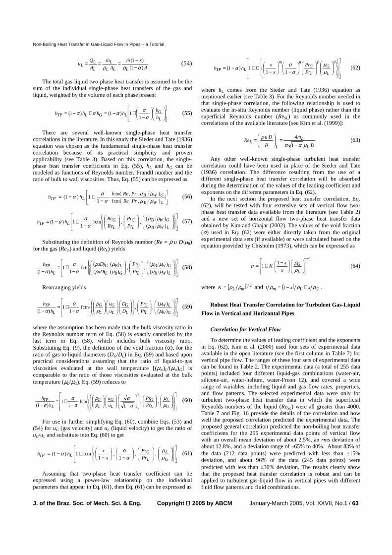
Non-Boiling Heat Transfer in Gas-Liquid Flow in Pipes – a Tutorial
J. of the Braz. Soc. of Mech. Sci. & Eng. Copyright 2005 by ABCM January-March 2005, Vol. XXVII, No.1 / 63
A
xm
A
m
A
Qu
LLL
L
L
LL )1(
)1(
αρρ −−===
&& (54)
The total gas-liquid two-phase heat transfer is assumed to be the
sum of the individual single-phase heat transfers of the gas and liquid, weighted by the volume of each phase present
−+−=+−=
L
GLGLTP h
hhhhh
ααααα
11)1()1( (55)
There are several well-known single-phase heat transfer
correlations in the literature. In this study the Sieder and Tate (1936) equation was chosen as the fundamental single-phase heat transfer correlation because of its practical simplicity and proven applicability (see Table 3). Based on this correlation, the single-phase heat transfer coefficients in Eq. (55), hL and hG can be modeled as functions of Reynolds number, Prandtl number and the ratio of bulk to wall viscosities. Thus, Eq. (55) can be expressed as
−+−=
LWB
GWBLTP PrRe
PrRehh
),,fctn(
),,fctn(
11)1(
µµµµ
ααα (56)
−+−=
LWB
GWB
L
G
L
GLTP Pr
Pr
Re
Rehh
)(
)(,,fctn
11)1(
µµµµ
ααα (57)
Substituting the definition of Reynolds number (Re = ρ u D/µB)
for the gas (ReG) and liquid (ReL) yields
−+=
− LWB
GWB
L
G
GB
LB
L
G
L
TP
Pr
Pr
uD
uD
h
h
)(
)(,,
)(
)(
)(
)(fctn
11
)1( µµµµ
µµ
ρρ
αα
α (58)
Rearranging yields
−+=
− GW
LW
L
G
L
G
L
G
L
G
L
TPPr
Pr
D
D
u
u
h
h
)(
)(,,fctn
11
)1( µµ
ρρ
αα
α (59)
where the assumption has been made that the bulk viscosity ratio in the Reynolds number term of Eq. (58) is exactly cancelled by the last term in Eq. (58), which includes bulk viscosity ratio. Substituting Eq. (9), the definition of the void fraction (α), for the ratio of gas-to-liquid diameters (DG/DL) in Eq. (59) and based upon practical considerations assuming that the ratio of liquid-to-gas viscosities evaluated at the wall temperature [(µW)L/(µW)G] is comparable to the ratio of those viscosities evaluated at the bulk temperature (µL/µG), Eq. (59) reduces to
−
−+=
− G
L
L
G
L
G
L
G
L
TP
Pr
Pr
u
u
h
h
µµ
αα
ρρ
αα
α,,
1fctn
11
)1( (60)
For use in further simplifying Eq. (60), combine Eqs. (53) and
(54) for uG (gas velocity) and uL (liquid velocity) to get the ratio of uG/uL and substitute into Eq. (60) to get
−
−+−=
G
L
L
GLTP Pr
Pr
x
xhh
µµ
ααα ,,
1,
1fctn1)1( (61)
Assuming that two-phase heat transfer coefficient can be
expressed using a power-law relationship on the individual parameters that appear in Eq. (61), then Eq. (61) can be expressed as
−
−+−=
q
L
Gp
L
Gnm
LTP Pr
Pr
x
xhh
µµ
ααα
11C1)1( (62)
where hL comes from the Sieder and Tate (1936) equation as mentioned earlier (see Table 3). For the Reynolds number needed in that single-phase correlation, the following relationship is used to evaluate the in-situ Reynolds number (liquid phase) rather than the superficial Reynolds number (ReSL) as commonly used in the correlations of the available literature [see Kim et al. (1999)]:
D
mDuRe
L
L
LL
µαπµρ
−=
=
1
4 & (63)
Any other well-known single-phase turbulent heat transfer
correlation could have been used in place of the Sieder and Tate (1936) correlation. The difference resulting from the use of a different single-phase heat transfer correlation will be absorbed during the determination of the values of the leading coefficient and exponents on the different parameters in Eq. (62).
In the next section the proposed heat transfer correlation, Eq. (62), will be tested with four extensive sets of vertical flow two-phase heat transfer data available from the literature (see Table 2) and a new set of horizontal flow two-phase heat transfer data obtained by Kim and Ghajar (2002). The values of the void fraction (α) used in Eq. (62) were either directly taken from the original experimental data sets (if available) or were calculated based on the equation provided by Chisholm (1973), which can be expressed as
1
11
−
−+=L
Gx
xK
ρρα (64)
where ( ) 21mLK ρρ= and ( ) GLm xx ρρρ +−= 11 .
Robust Heat Transfer Correlation for Turbulent Gas-Liquid
Flow in Vertical and Horizontal Pipes
Correlation for Vertical Flow
To determine the values of leading coefficient and the exponents in Eq. (62), Kim et al. (2000) used four sets of experimental data available in the open literature (see the first column in Table 7) for vertical pipe flow. The ranges of these four sets of experimental data can be found in Table 2. The experimental data (a total of 255 data points) included four different liquid-gas combinations (water-air, silicone-air, water-helium, water-Freon 12), and covered a wide range of variables, including liquid and gas flow rates, properties, and flow patterns. The selected experimental data were only for turbulent two-phase heat transfer data in which the superficial Reynolds numbers of the liquid (ReSL) were all greater than 4000. Table 7 and Fig. 16 provide the details of the correlation and how well the proposed correlation predicted the experimental data. The proposed general correlation predicted the non-boiling heat transfer coefficients for the 255 experimental data points of vertical flow with an overall mean deviation of about 2.5%, an rms deviation of about 12.8%, and a deviation range of –65% to 40%. About 83% of the data (212 data points) were predicted with less than ±15% deviation, and about 96% of the data (245 data points) were predicted with less than ±30% deviation. The results clearly show that the proposed heat transfer correlation is robust and can be applied to turbulent gas-liquid flow in vertical pipes with different fluid flow patterns and fluid combinations.
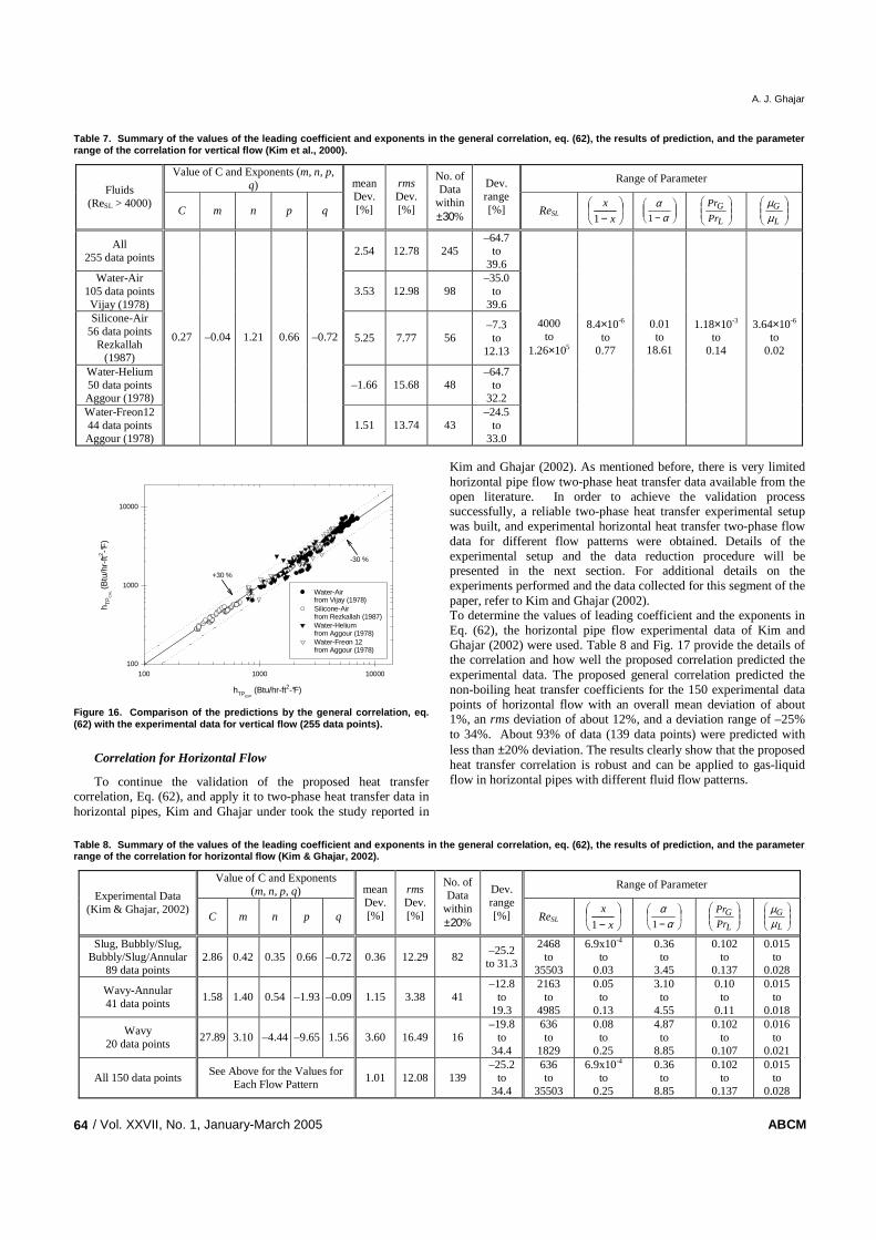
A. J. Ghajar
/ Vol. XXVII, No. 1, January-March 2005 ABCM 64
Table 7. Summary of the values of the leading coef ficient and exponents in the general correlation, e q. (62), the results of prediction, and the paramet er range of the correlation for vertical flow (Kim et al., 2000).
Value of C and Exponents (m, n, p, q)
Range of Parameter Fluids
(ReSL > 4000) C m n p q
mean Dev. [%]
rms Dev. [%]
No. of Data
within ±30%
Dev. range [%] ReSL
− x
x
1
− αα
1
L
G
Pr
Pr
L
G
µµ
All 255 data points
2.54 12.78 245 –64.7
to 39.6
Water-Air 105 data points Vijay (1978)
3.53 12.98 98 –35.0
to 39.6
Silicone-Air 56 data points
Rezkallah (1987)
5.25 7.77 56 –7.3 to
12.13
Water-Helium 50 data points Aggour (1978)
–1.66 15.68 48 –64.7
to 32.2
Water-Freon12 44 data points Aggour (1978)
0.27 –0.04 1.21 0.66 –0.72
1.51 13.74 43 –24.5
to 33.0
4000 to
1.26×10⁵
8.4×10⁻⁶ to
0.77
0.01 to
18.61
1.18×10⁻³ to
0.14
3.64×10⁻⁶ to
0.02
hTPEXP (Btu/hr-ft2-°F)
100 1000 10000
h TP
CA
L (B
tu/h
r-ft2 -°F
)
100
1000
10000
Water-Airfrom Vijay (1978)Silicone-Airfrom Rezkallah (1987)Water-Heliumfrom Aggour (1978)Water-Freon 12from Aggour (1978)
+30 %
-30 %
Figure 16. Comparison of the predictions by the ge neral correlation, eq. (62) with the experimental data for vertical flow ( 255 data points).
Correlation for Horizontal Flow
To continue the validation of the proposed heat transfer correlation, Eq. (62), and apply it to two-phase heat transfer data in horizontal pipes, Kim and Ghajar under took the study reported in
Kim and Ghajar (2002). As mentioned before, there is very limited horizontal pipe flow two-phase heat transfer data available from the open literature. In order to achieve the validation process successfully, a reliable two-phase heat transfer experimental setup was built, and experimental horizontal heat transfer two-phase flow data for different flow patterns were obtained. Details of the experimental setup and the data reduction procedure will be presented in the next section. For additional details on the experiments performed and the data collected for this segment of the paper, refer to Kim and Ghajar (2002). To determine the values of leading coefficient and the exponents in Eq. (62), the horizontal pipe flow experimental data of Kim and Ghajar (2002) were used. Table 8 and Fig. 17 provide the details of the correlation and how well the proposed correlation predicted the experimental data. The proposed general correlation predicted the non-boiling heat transfer coefficients for the 150 experimental data points of horizontal flow with an overall mean deviation of about 1%, an rms deviation of about 12%, and a deviation range of –25% to 34%. About 93% of data (139 data points) were predicted with less than ±20% deviation. The results clearly show that the proposed heat transfer correlation is robust and can be applied to gas-liquid flow in horizontal pipes with different fluid flow patterns.
Table 8. Summary of the values of the leading coef ficient and exponents in the general correlation, e q. (62), the results of prediction, and the paramet er range of the correlation for horizontal flow (Kim & Ghajar, 2002).
Value of C and Exponents (m, n, p, q)
Range of Parameter Experimental Data
(Kim & Ghajar, 2002) C m n p q
mean Dev. [%]
rms Dev. [%]
No. of Data
within ±20%
Dev. range [%] ReSL
− x
x
1
− αα
1
L
GPr
Pr
L
Gµµ
Slug, Bubbly/Slug, Bubbly/Slug/Annular
89 data points 2.86 0.42 0.35 0.66 –0.72 0.36 12.29 82
–25.2 to 31.3
2468 to
35503
6.9x10⁻⁴ to
0.03
0.36 to
3.45
0.102 to
0.137
0.015 to
0.028
Wavy-Annular 41 data points
1.58 1.40 0.54 –1.93 –0.09 1.15 3.38 41 –12.8
to 19.3
2163 to
4985
0.05 to
0.13
3.10 to
4.55
0.10 to
0.11
0.015 to
0.018
Wavy 20 data points
27.89 3.10 –4.44 –9.65 1.56 3.60 16.49 16 –19.8
to 34.4
636 to
1829
0.08 to
0.25
4.87 to
8.85
0.102 to
0.107
0.016 to
0.021
All 150 data points See Above for the Values for
Each Flow Pattern 1.01 12.08 139
–25.2 to
34.4
636 to
35503
6.9x10⁻⁴ to
0.25
0.36 to
8.85
0.102 to
0.137
0.015 to
0.028

Non-Boiling Heat Transfer in Gas-Liquid Flow in Pipes – a Tutorial
J. of the Braz. Soc. of Mech. Sci. & Eng. Copyright 2005 by ABCM January-March 2005, Vol. XXVII, No.1 / 65
hTPEXP (Btu/hr-ft2-°F)
100 1000
h TP
CA
L (B
tu/h
r-ft2 -°F
)
100
1000
+30 %
-30 %
+20 %
-20 %
Figure 17. Comparison of the predictions by genera l correlation, eq. (62) with the experimental data for horizontal flow (150 data points).
Experimental Setup and Data Reduction for Horizontal and
Slightly Upward Inclined Pipe Flows
A schematic diagram of the overall experimental setup for heat transfer and pressure drop measurements and flow visualizations in two-phase air-water pipe flow in horizontal and inclined positions is shown in Fig. 18. The test section is a 27.9 mm straight standard stainless steel schedule 10S pipe with a length to diameter ratio of a 100. The setup rests atop an aluminum I-beam that is supported by a pivoting foot and a stationary foot that incorporates a small electric screw jack. The I-beam is approximately 9 m in length and can be inclined to an angle of approximately 8° above horizontal. Inclination angles of the test cradle are measured with a contractor’s angle-measuring tool and with a digital x-y axis accelerometer to determine the angle to within 0.5°.
Figure 18. Schematic of experimental setup.
In order to apply uniform wall heat flux boundary conditions to
the test section, copper plates were silver soldered to the inlet and exit of the test section. The uniform wall heat flux boundary condition was maintained by a Lincoln SA-750 welder. The entire length of the test section was wrapped using fiberglass pipe wrap insulation, followed by a thin polymer vapor seal to prevent moisture penetration.
In order to develop various two-phase flow patterns (by controlling the flow rates of gas and liquid), a two-phase gas and
liquid flow mixer was used. The mixer consisted of a perforated stainless steel tube (6.35 mm I.D.) inserted into the liquid stream by means of a tee and a compression fitting. The end of the copper tube was silver-soldered. Four holes (3 rows of 1.59 mm, 4 rows of 3.18 mm, and 8 rows of 3.97 mm) were positioned at 90° intervals around the perimeter of the tube and this pattern was repeated at fifteen equally spaced axial locations along the length of the stainless steel tube (refer to Fig. 19). The two-phase flow leaving mixer entered the transparent calming section.
The calming section [clear polycarbonate pipe with 25.4 mm I.D. and L/D = 88] served as a flow developing and turbulence reduction device, and flow pattern observation section. One end of the calming section is connected to the test section with an acrylic flange and the other end of the calming section is connected to the gas-liquid mixer. For the horizontal flow measurements, the test section and the observation section (refer to Fig. 18) were carefully leveled to eliminate the effect of inclination on these measurements.
Figure 19. Air-water mixer.
Holes for eleven pressure taps were drilled along the test section
(refer to Fig. 20). The diameters of the holes were 1.73 mm, and were equally spaced at 254 mm intervals along the test section. The holes were located at the bottom of the stainless steel tube in order to ensure that only water could get into the pressure measuring system. The pressure taps were standard saddle type self-tapping valves with the tapping core removed. The first pressure tap in the flow direction was used as a reference pressure tap for comparison with the other pressure taps; and the system pressure was measured by an OMEGA PX242-060G pressure transducer which had a 0 to 60 psig operation range. The reference pressure tap was also directly connected to a VALIDYNE DP15 wet-wet differential pressure transducer with CD15 carrier demodulator. The pressure tap desired to measure the differential pressure among the other 10 pressure taps was connected to the differential pressure transducer in isothermal condition. Note that the pressure measurements are not reported in this paper.
Figure 20. Test section.

A. J. Ghajar
/ Vol. XXVII, No. 1, January-March 2005 ABCM 66
T-type thermocouple wires were cemented with Omegabond 101, an epoxy adhesive with high thermal conductivity and electrical resistivity, to the outside wall of the stainless steel test section (refer to Fig. 20). Omega EXPP-T-20-TWSH extension wires were used for relay to the data acquisition system. Thermocouples were placed on the outer surface of the tube wall at uniform intervals of 254 mm from the entrance to the exit of the test section. There were 10 thermocouple stations in the test section. All stations had four thermocouples, and they were labeled looking at the tail of the fluid flow with peripheral location “A” being at the top of the tube, “B” being 90° in the clockwise direction, “C” at the bottom of the tube, and “D” being 90° from the bottom in the clockwise sense (refer to Fig. 20). All the thermocouples were monitored with a National Instruments data acquisition system. The experimental data were averaged over a user chosen length of time (typically 20 samples/channel with a sampling rate of 400 scans/sec) before the heat transfer measurements were actually recorded. The average system stabilization time period was from 30 to 60 min after the system attained steady state. The inlet liquid and gas temperatures and the exit bulk temperature were measured by Omega TMQSS-125U-6 thermocouple probes. The thermocouple probe for the exit bulk temperature was placed after the mixing well. Calibration of thermocouples and thermocouple probes showed that they were accurate within ±0.5°C. The operating pressures inside the experimental setup were monitored with a pressure transducer.
To ensure a uniform fluid bulk temperature at the inlet and exit of the test section, a mixing well was utilized. An alternating polypropylene baffle type static mixer for both gas and liquid phases was used. This mixer provided an overlapping baffled passage forcing the fluid to encounter flow reversal and swirling regions. The mixing well at the exit of the test section was placed below the clear polycarbonate observation section (after the test section), and before the liquid storage tank (refer to Fig. 18). Since the cross-sectional flow passage of the mixing section was substantially smaller than the test section, it had the potential of increasing the system back-pressure. Thus, in order to reduce the potential back-pressure problem, which might affect the flow pattern inside of the test section, the mixing well was placed below and after the test section and the clear observation sections. The outlet bulk temperature was measured immediately after the mixing well.
The fluids used in the test loop are air and water. The water is distilled and stored in a 55-gallon cylindrical polyethylene tank. A Bell & Gosset series 1535 coupled centrifugal pump was used to pump the water through an Aqua-Pure AP12T water filter. An ITT Standard model BCF 4063 one shell and two-tube pass heat exchanger removes the pump heat and the heat added during the test to maintain a constant inlet water temperature. From the heat exchanger, the water passes through a Micro Motion Coriolis flow meter (model CMF125) connected to a digital Field-Mount Transmitter (model RFT9739) that conditions the flow information for the data acquisition system. Once the water passes through the Coriolis flow meter it then passes through a 25.4 mm, twelve-turn gate valve that regulates the amount of flow that entered the test section. From this point, the water travels through a 25.4 mm flexible hose, through a one-way check valve, and into the test section. Air is supplied via an Ingersoll-Rand T30 (model 2545) industrial air compressor mounted outside the laboratory and isolated to reduce vibration onto the laboratory floor. The air passes through a copper coil submerged in a vessel of water to lower the temperature of the air to room temperature. The air is then filtered and condensate removed in a coalescing filter. The air flow is measured by a Micro Motion Coriolis flow meter (model CMF100) connected to a digital Field-Mount Transmitter (model RFT9739) and regulated by a needle valve. Air is delivered to the test section
by flexible tubing. The water and air mixture is returned to the reservoir where it is separated and the water recycled.
The heat transfer measurements at uniform wall heat flux boundary condition were carried out by measuring the local outside wall temperatures at 10 stations along the axis of the tube and the inlet and outlet bulk temperatures in addition to other measurements such as the flow rates of gas and liquid, room temperature, voltage drop across the test section, and current carried by the test section. The peripheral heat transfer coefficient (local average) were calculated based on the knowledge of the pipe inside wall surface temperature and inside wall heat flux obtained from a data reduction program developed exclusively for this type of experiments (Ghajar and Zurigat, 1991). The local average peripheral values for inside wall temperature, inside wall heat flux, and heat transfer coefficient were then obtained by averaging all the appropriate individual local peripheral values at each axial location. The large variation in the circumferential wall temperature distribution, which is typical for two-phase gas-liquid flow in horizontal and slightly inclined tubes, leads to different heat transfer coefficients depending on which circumferential wall temperature was selected for the calculations. In two-phase heat transfer experiments, in order to overcome the unbalanced circumferential heat transfer coefficients, Eq. (52) was used to calculate an overall mean two-phase heat transfer coefficient (hTP) for each test run.
The data reduction program used a finite-difference formulation to determine the inside wall temperature and the inside wall heat flux from measurements of the outside wall temperature, the heat generation within the pipe wall, and the thermophysical properties of the pipe material (electrical resistivity and thermal conductivity). In these calculations, axial conduction was assumed negligible, but peripheral and radial conduction of heat in the tube wall were included. In addition, the bulk fluid temperature was assumed to increase linearly from the inlet to outlet, see section 5.3 for additional details.
A National Instruments data acquisition system was used to record and store the data measured during these experiments. The acquisition system is housed in an AC powered four-slot SCXI 1000 Chassis that serves as a low noise environment for signal conditioning. Three NI SCXI control modules are housed inside the chassis. There are two SCXI 1102/B/C modules and one SCXI 1125 module. From these three modules, input signals for all 40 thermocouples, the two thermocouple probes, voltmeter, and flow meters are gathered and recorded. The computer interface used to record the data is a LabVIEW Virtual Instrument (VI) program written for this specific application.
The reliability of the flow circulation system and of the experimental procedures was checked by making several single-phase calibration runs with distilled water. The single-phase heat transfer experimental data were checked against the well established single-phase heat transfer correlations (Kim and Ghajar, 2002) in the Reynolds number range from 3000 to 30,000. In most instances, the majority of the experimental results were well within ±10% of the predicted results (Kim and Ghajar, 2002; Durant, 2003). In addition to the single-phase calibration runs, a series of two-phase, air-water, slug flow tests were also performed for comparison against the two-phase experimental slug flow data of (Durant, 2003; Trimble et al., 2002). The results of these comparisons, for majority of the cases were also well within the ±10% deviation range.
The uncertainty analyses of the overall experimental procedures using the method of Kline and McClintock (1953) showed that there is a maximum of 11.5% uncertainty for heat transfer coefficient calculations. Experiments under the same conditions were conducted periodically to ensure the repeatability of the results. The maximum difference between the duplicated experimental runs was

Non-Boiling Heat Transfer in Gas-Liquid Flow in Pipes – a Tutorial
J. of the Braz. Soc. of Mech. Sci. & Eng. Copyright 2005 by ABCM January-March 2005, Vol. XXVII, No.1 / 67
within ±10%. More details of experimental setup and data reduction procedures can be found from Durant (2003).
The heat transfer data obtained with the present experimental setup were measured under a uniform wall heat flux boundary condition that ranged from 2606 to 10,787 W/m2 and the resulting mean two-phase heat transfer coefficients (hTP) ranged from 545 to 4907 W/m2⋅K. For these experiments, the liquid superficial Reynolds numbers (ReSL) ranged from 836 to 26,043 (water mass flow rates from about 1.18 to 42.5 kg/min) and the gas superficial Reynolds numbers (ReSG) ranged from 560 to 47,718 (gas mass flow rates from about 0.013 to 1.13 kg/min).
Flow Patterns
Due to the multitude of flow patterns and the various interpretations accorded to them by different investigators, no uniform procedure exists at present for describing and classifying them. In our reported studies the flow pattern identification for the experimental data was based on the procedures suggested by Kim and Ghajar (2002) and visual observations deemed appropriate. All observations for the flow pattern judgments were made at two locations, just before the test section (about L/D = 93 in the calming section from the mixing well, see Fig. 19) and right after the test section. Leaving the liquid flow rate fixed, flow patterns were observed for various air flow rates. The liquid flow rate was then adjusted and the process was repeated. If the observed flow patterns differed at the two locations of before and after the test section, experimental data was not taken and the flow rates of gas and liquid were readjusted for consistent flow pattern observations. Flow pattern data were obtained with the pipe at horizontal position and at 2°, 5°, and 7° upward inclined positions. These experimental data were plotted and compared using their corresponding values of mass flow rates of air and water and the flow patterns. The digital images of each flow pattern at each inclination angle were also compared with each other in order to identify the inclination effect on the flow pattern.
Figure 22 ows photographs of the representative flow patterns that were observed in our experimental setup with the pipe in the horizontal position and no heating (isothermal runs). Figure 22 shows the flow map for our pipe in the horizontal position. The different flow patterns depicted on this figure illustrate the capability of our experimental setup in producing multitude of flow patterns. The shaded regions represent the boundaries of these flow patterns for the pipe in the horizontal position. Also shown on Fig.
(a) Stratified
(b) Plug
(c) Slug
(d) Wavy
Figure 21. Photographs of representative flow patt erns (horizontal flow and isothermal).
(e) Bubbly/Slug
(f) Annular/Bubbly/Slug
(g) Annular/Wavy
(h) Annular
Figure 21. (Continued).
Figure 22. Flow map for horizontal flow.
24 with symbols is the distribution of the heat transfer data that were obtained systematically in our experimental setup with the pipe in the horizontal position. As can be seen from Fig. 24, we did not collect heat transfer data at low air and water flow rate combinations (water flow rates of less than about 5 kg/min and air flow rates of less than about 0.5 kg/min). At these low water and air flow rates and heating there is a strong possibility of either dry-out or local boiling which could damage the test section.
As mentioned in Fig. 24, there are very few flow pattern data and flow pattern maps available in the literature for tubes with small angles of inclination. The influence of small upward inclination angles of 2°, 5°, and 7° on the observed flow patterns is shown in Fig. 25Error! Reference source not found.. This figure is a modified version of Fig. 24, which is based on the mass flow rate of each phase. As shown in Fig. 25, the shaded regions representing the transition boundaries of the flow patterns have shifted to the upper left direction for plug-slug and slug-bubbly/slug transition due to the different inclination angles. The annular/bubbly/slug-annular

A. J. Ghajar
/ Vol. XXVII, No. 1, January-March 2005 ABCM 68
transition boundaries appear to be insensitive to the slight inclination angles studied in this study. There are no drastic changes in the transition boundaries at the upward inclination angles of 2°, 5°, and 7° compared to the horizontal orientation. However, it should be mentioned that even though the flow pattern is named the same for both horizontal and inclined flows; it does not mean that the flow pattern in the inclined position has identical characteristics of the comparable flow pattern in the horizontal position. For example, it is observed that the slug flow patterns in the inclined positions of 5° and 7° have reverse flow between slugs due to the gravitational force, which can have a significant effect on the heat transfer.
Figure 23. Change of flow pattern transition lines as pipe inclined upward from horizontal.
Note that we have not taken flow pattern data below the liquid
flow rate of about 5 kg/min for the inclined cases. Therefore, at this time we have no information on the influence of inclination angle on the flow pattern in this area. This is the subject of our near future investigations.
Systematic Investigation on Two-Phase Gas-Liquid Heat
Transfer in Horizontal and Slightly Upward Inclined Pipe Flows
In this section we present an overview of the different trends that we have observed in the heat transfer behavior of the two-phase air-water flow in horizontal and inclined pipes for a variety of flow patterns. The two-phase heat transfer data were obtained by systematically varying the air or water flow rates and the pipe inclination angle.
Figure 26 provides an overview of the pronounced influence of the flow pattern, superficial liquid Reynolds number (water flow rate) and superficial gas Reynolds number (air flow rate) on the two-phase mean heat transfer coefficient in horizontal pipe flows. The results presented in Fig. 26(a) clearly show that two-phase mean heat transfer coefficients are strongly influenced by the liquid superficial Reynolds number (ReSL). As shown in Fig. 26(a), the heat transfer coefficient increases proportionally as ReSL increases. In addition, for a fixed ReSL, the two-phase mean heat transfer coefficients are also influenced by the gas superficial Reynolds number (ReSG) and each flow pattern shows its own distinguished heat transfer trend as shown in Fig. 26(b). Typically, heat transfer increases at low ReSG (the regime of plug flow), and then slightly decreases at the mid range of ReSG (the regime of slug and slug-type
transitional flows), and again increases at the high ReSG (the regime of annular flow).
ReSL
0 5000 10000 15000 20000 25000 30000
h TP
EX
P [W
/m2 K
]
0
1000
2000
3000
4000
5000
6000Flow Pattern
PlugSlug & Slug/BubblySlug/WavyWavy/AnnularSlug/Bubbly/AnnularAnnular
(a) hTP vs. ReSL
ReSG X 10-3
0.6 0.8 2 4 6 8 20 40 601 10
h TP
EX
P [W
/m2 -K
]
0
1000
2000
3000
4000
5000
600026000220001700015000120009500700050001500850
ReSL
Flow Pattern
PlugSlug & Slug/BubblySlug/WavyWavy/AnnularSlug/Bubbly/AnnularAnnular
(b) hTP vs. ReSG
Figure 24. Variation of two-phase heat transfer co efficients with superficial liquid and gas reynolds numbers in a horizontal flow.
ReSL = 5000
ReSG
1000 10000 100000
h TP
EX
P [W
/m2 -K
]
0
1000
2000
3000
4000
Horizontal2 Degrees5 Degrees7 Degrees
(a) ReSL = 5000
ReSL = 12000
ReSG
1000 10000 100000
h TP
EX
P [W
/m2-K
]
0
1000
2000
3000
4000
Horizontal2 Degrees5 Degrees7 Degrees
(b) ReSL = 12000
Figure 25. Inclination effects on overall mean hea t transfer coefficients.
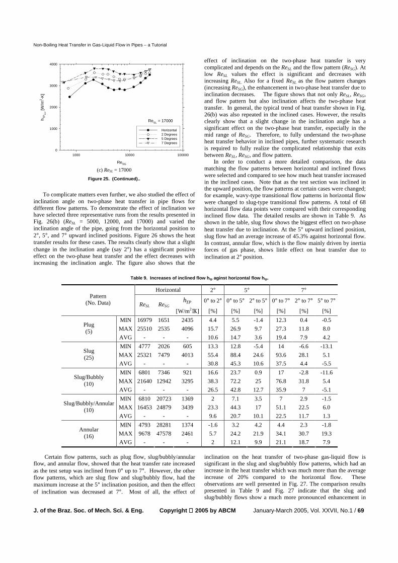
Non-Boiling Heat Transfer in Gas-Liquid Flow in Pipes – a Tutorial
J. of the Braz. Soc. of Mech. Sci. & Eng. Copyright 2005 by ABCM January-March 2005, Vol. XXVII, No.1 / 69
ReSL = 17000
ReSG
1000 10000 100000
h TP
EX
P [W
/m2 -K
]
0
1000
2000
3000
4000
Horizontal2 Degrees5 Degrees7 Degrees
(c) ReSL = 17000
Figure 25. (Continued)..
To complicate matters even further, we also studied the effect of
inclination angle on two-phase heat transfer in pipe flows for different flow patterns. To demonstrate the effect of inclination we have selected three representative runs from the results presented in Fig. 26(b) (ReSL = 5000, 12000, and 17000) and varied the inclination angle of the pipe, going from the horizontal position to 2°, 5°, and 7° upward inclined positions. Figure 26 shows the heat transfer results for these cases. The results clearly show that a slight change in the inclination angle (say 2°) has a significant positive effect on the two-phase heat transfer and the effect decreases with increasing the inclination angle. The figure also shows that the
effect of inclination on the two-phase heat transfer is very complicated and depends on the ReSL and the flow pattern (ReSG). At low ReSL values the effect is significant and decreases with increasing ReSL. Also for a fixed ReSL as the flow pattern changes (increasing ReSG), the enhancement in two-phase heat transfer due to inclination decreases. The figure shows that not only ReSL, ReSG, and flow pattern but also inclination affects the two-phase heat transfer. In general, the typical trend of heat transfer shown in Fig. 26(b) was also repeated in the inclined cases. However, the results clearly show that a slight change in the inclination angle has a significant effect on the two-phase heat transfer, especially in the mid range of ReSG. Therefore, to fully understand the two-phase heat transfer behavior in inclined pipes, further systematic research is required to fully realize the complicated relationship that exits between ReSL, ReSG, and flow pattern.
In order to conduct a more detailed comparison, the data matching the flow patterns between horizontal and inclined flows were selected and compared to see how much heat transfer increased in the inclined cases. Note that as the test section was inclined in the upward position, the flow patterns at certain cases were changed; for example, wavy-type transitional flow patterns in horizontal flow were changed to slug-type transitional flow patterns. A total of 68 horizontal flow data points were compared with their corresponding inclined flow data. The detailed results are shown in Table 9. As shown in the table, slug flow shows the biggest effect on two-phase heat transfer due to inclination. At the 5° upward inclined position, slug flow had an average increase of 45.3% against horizontal flow. In contrast, annular flow, which is the flow mainly driven by inertia forces of gas phase, shows little effect on heat transfer due to inclination at 2° position.
Table 9. Increases of inclined flow htp aginst horizontal flow htp.
Horizontal 2° 5° 7°
TPh 0° to 2° 0° to 5° 2° to 5° 0° to 7° 2° to 7° 5° to 7° Pattern
(No. Data) ReSL ReSG [W/m2⋅K] [%] [%] [%] [%] [%] [%]
MIN 16979 1651 2435 4.4 5.5 -1.4 12.3 0.4 -0.5
MAX 25510 2535 4096 15.7 26.9 9.7 27.3 11.8 8.0 Plug (5)
AVG - - - 10.6 14.7 3.6 19.4 7.9 4.2
MIN 4777 2026 605 13.3 12.8 -5.4 14 -6.6 -13.1
MAX 25321 7479 4013 55.4 88.4 24.6 93.6 28.1 5.1 Slug (25)
AVG - - - 30.8 45.3 10.6 37.5 4.4 -5.5
MIN 6801 7346 921 16.6 23.7 0.9 17 -2.8 -11.6
MAX 21640 12942 3295 38.3 72.2 25 76.8 31.8 5.4 Slug/Bubbly
(10) AVG - - - 26.5 42.8 12.7 35.9 7 -5.1
MIN 6810 20723 1369 2 7.1 3.5 7 2.9 -1.5
MAX 16453 24879 3439 23.3 44.3 17 51.1 22.5 6.0 Slug/Bubbly/Annular
(10) AVG - - - 9.6 20.7 10.1 22.5 11.7 1.3
MIN 4793 28281 1374 -1.6 3.2 4.2 4.4 2.3 -1.8
MAX 9678 47578 2461 5.7 24.2 21.9 34.1 30.7 19.3 Annular
(16) AVG - - - 2 12.1 9.9 21.1 18.7 7.9
Certain flow patterns, such as plug flow, slug/bubbly/annular
flow, and annular flow, showed that the heat transfer rate increased as the test setup was inclined from 0° up to 7°. However, the other flow patterns, which are slug flow and slug/bubbly flow, had the maximum increase at the 5° inclination position, and then the effect of inclination was decreased at 7°. Most of all, the effect of
inclination on the heat transfer of two-phase gas-liquid flow is significant in the slug and slug/bubbly flow patterns, which had an increase in the heat transfer which was much more than the average increase of 20% compared to the horizontal flow. These observations are well presented in Fig. 27. The comparison results presented in Table 9 and Fig. 27 indicate that the slug and slug/bubbly flows show a much more pronounced enhancement in

A. J. Ghajar
/ Vol. XXVII, No. 1, January-March 2005 ABCM 70
the two-phase heat transfer at all inclination angles in comparison to the other flow patterns shown (plug flow, slug/bubbly/annular flow, annular flow). The difference between the two groups of flow patterns has to do with the degree of mixing between each phase and the inertia force carried by each phase against the buoyancy force.
Flow Pattern
PLUG SLUG BS ABS ANNULAR
Incr
ease
s in
hT
P a
gain
st H
oriz
onta
l Flo
w [%
]
0
10
20
30
40
50
2 deg5 deg7 deg
Figure 26. Increases of inclined flow htp against horizontal flow htp .
For a more detailed look at the effect of inclination on heat
transfer in two-phase gas-liquid flow, the increase in hTP versus ReSL for each flow pattern is presented in Fig. 27. As shown in the figure, except for the case of annular flow, all other flow patterns indicated that the effect of the inclination at low ReSL was significantly high and then decreased with increasing ReSL. In the case of slug flow, the increase in the heat transfer was as much as 94% at ReSL of around 5000 and at the 5° inclined position. However, it dropped to around 13% at ReSL of around 25,000. This drop can be expressed as a drastic change in the effect of inclination on the heat transfer. The other flow patterns, except annular flow, show a similar trend as that of slug flow. These trends show that the increase of the inertia force in the fluid phases suppresses the effect of inclination.
Plug
ReSL
0 5000 10000 15000 20000 25000 30000
Incr
ease
s in
hT
P a
gain
st H
oriz
onta
l Flo
w [%
]
-20
0
20
40
60
80
100
2 deg5 deg7 deg
Annular
(a) annular flow and plug flow
Slug
ReSL
0 5000 10000 15000 20000 25000 30000
Incr
ease
s in
hT
P a
gain
st H
oriz
onta
l Flo
w [%
]
-20
0
20
40
60
80
100
2 deg5 deg7 deg
(b) slug flow
Figure 27. Increases of inclined flow h tp against horizontal flow h tp by flow pattern.
Slug/Bubbly
ReSL
0 5000 10000 15000 20000 25000 30000
Incr
ease
s in
hT
P a
gain
st H
oriz
onta
l Flo
w [%
]
-20
0
20
40
60
80
100
2 deg5 deg7 deg
(c) slug/bubbly flow
Slug/Bubbly/Annular
ReSL
0 5000 10000 15000 20000 25000 30000
Incr
ease
s in
hT
P a
gain
st H
oriz
onta
l Flo
w [%
]
-20
0
20
40
60
80
100
2 deg5 deg7 deg
(d) slug/bubbly/annular flow
Figure 27. (Continued).
The effect of inclination on heat transfer in non-boiling two-
phase gas-liquid flow has been presented in many ways to better understand the mechanisms involved. As presented in this section, heat transfer in non-boiling two-phase gas-liquid flow is influenced by each of ReSL, ReSG, flow pattern, and inclination angle in a very complicated way. With increasing ReSL, heat transfer proportionally increased regardless of the rest of the factors. By varying ReSG, the distinguished trends of heat transfer by flow patterns were observed. Furthermore, significant changes were observed in the two-phase heat transfer of air-water flow with a slight upward inclination of the pipe from the horizontal position.
The inclined heat transfer results presented in this section for the different flow patterns shed some light on the effect of inclination angle on the two-phase heat transfer for different flow patterns, and at the time raises a few additional questions. What is the relationship among the inclination angle, the flow pattern, and heat transfer? How much enhancement for a specific flow pattern should one expect due to inclination? What is optimum inclination angle for enhancement? These questions require systematic heat transfer measurements for a variety of flow patterns and inclination angles.
Heat Transfer Correlations for Horizontal and Incli ned Slug
and Annular Flows
In an earlier section of this paper we presented a two-phase heat transfer correlation for horizontal flow in pipes, see Eq. (62) and Table 8. In this section we will continue that effort by modifying our proposed general heat transfer correlation to account for inclination effect on two-phase heat transfer. For this purpose we will use our horizontal and inclined slug and annular flow heat transfer results presented and discussed in conjunction with Figs. 26 to 27. The modified form of our general correlation, Eq. (62) with inclusion of an inclination factor is:
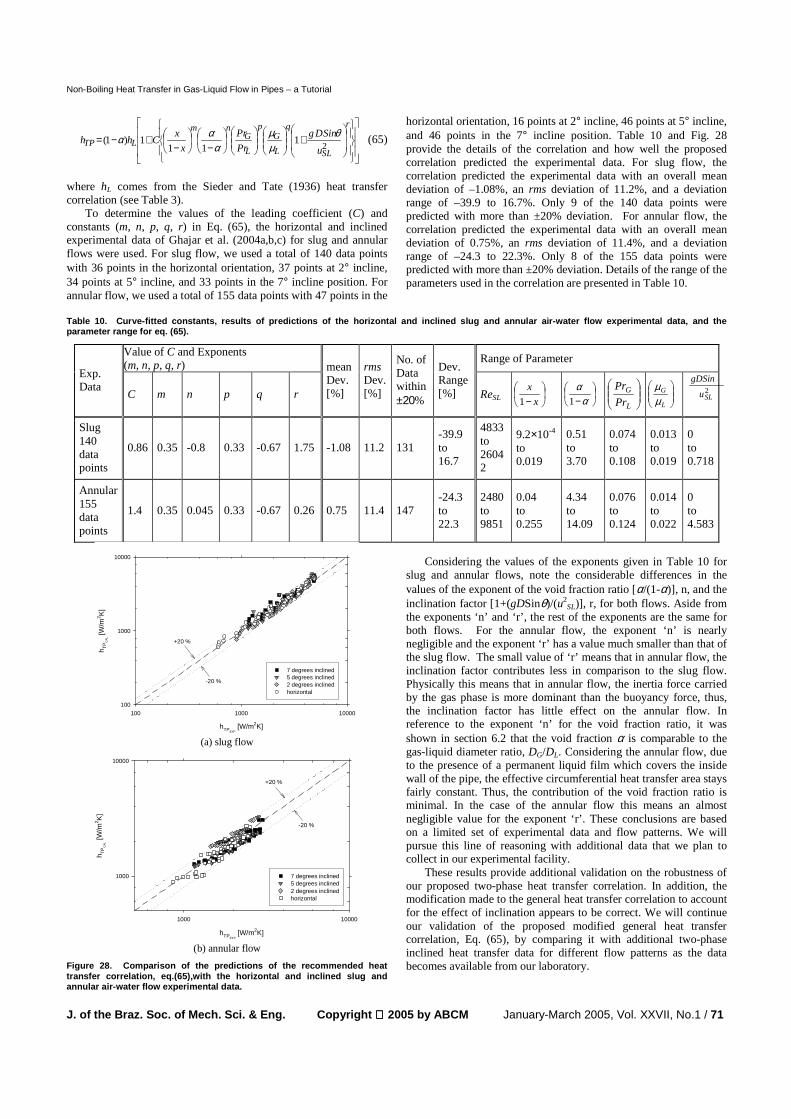
Non-Boiling Heat Transfer in Gas-Liquid Flow in Pipes – a Tutorial
J. of the Braz. Soc. of Mech. Sci. & Eng. Copyright 2005 by ABCM January-March 2005, Vol. XXVII, No.1 / 71
+
−
−+−=
r
SL
q
L
Gp
L
Gnm
LTPu
SinDg
Pr
Pr
x
xChh
21
111)1(
θµµ
ααα (65)
where hL comes from the Sieder and Tate (1936) heat transfer correlation (see Table 3).
To determine the values of the leading coefficient (C) and constants (m, n, p, q, r) in Eq. (65), the horizontal and inclined experimental data of Ghajar et al. (2004a,b,c) for slug and annular flows were used. For slug flow, we used a total of 140 data points with 36 points in the horizontal orientation, 37 points at 2° incline, 34 points at 5° incline, and 33 points in the 7° incline position. For annular flow, we used a total of 155 data points with 47 points in the
horizontal orientation, 16 points at 2° incline, 46 points at 5° incline, and 46 points in the 7° incline position. Table 10 and Fig. 28 provide the details of the correlation and how well the proposed correlation predicted the experimental data. For slug flow, the correlation predicted the experimental data with an overall mean deviation of –1.08%, an rms deviation of 11.2%, and a deviation range of –39.9 to 16.7%. Only 9 of the 140 data points were predicted with more than ±20% deviation. For annular flow, the correlation predicted the experimental data with an overall mean deviation of 0.75%, an rms deviation of 11.4%, and a deviation range of –24.3 to 22.3%. Only 8 of the 155 data points were predicted with more than ±20% deviation. Details of the range of the parameters used in the correlation are presented in Table 10.
Table 10. Curve-fitted constants, results of predi ctions of the horizontal and inclined slug and annu lar air-water flow experimental data, and the parameter range for eq. (65).
Value of C and Exponents (m, n, p, q, r)
Range of Parameter Exp. Data
C m n p q r
mean Dev. [%]
rms Dev. [%]
No. of Data within ±20%
Dev. Range [%] ReSL
− x
x
1
−αα
1
L
G
Pr
Pr
L
G
µµ 2
SLu
gDSinθ
Slug 140 data points
0.86 0.35 -0.8 0.33 -0.67 1.75 -1.08 11.2 131 -39.9 to 16.7
4833 to 26042
9.2×10⁻⁴ to 0.019
0.51 to 3.70
0.074 to 0.108
0.013 to 0.019
0 to 0.718
Annular 155 data points
1.4 0.35 0.045 0.33 -0.67 0.26 0.75 11.4 147 -24.3 to 22.3
2480 to 9851
0.04 to 0.255
4.34 to 14.09
0.076 to 0.124
0.014 to 0.022
0 to 4.583
hTPEXP [W/m2K]
100 1000 10000
h TP
CA
L [W/m
2 K]
100
1000
10000
7 degrees inclined5 degrees inclined2 degrees inclinedhorizontal
+20 %
-20 %
(a) slug flow
hTPEXP [W/m2K]
1000 10000
h TP
CA
L [W/m
2 K]
1000
10000
7 degrees inclined5 degrees inclined2 degrees inclinedhorizontal
+20 %
-20 %
(b) annular flow
Figure 28. Comparison of the predictions of the re commended heat transfer correlation, eq.(65),with the horizontal a nd inclined slug and annular air-water flow experimental data.
Considering the values of the exponents given in Table 10 for
slug and annular flows, note the considerable differences in the values of the exponent of the void fraction ratio [α/(1-α)], n, and the inclination factor [1+(gDSinθ)/(u2
SL)], r, for both flows. Aside from the exponents ‘n’ and ‘r’, the rest of the exponents are the same for both flows. For the annular flow, the exponent ‘n’ is nearly negligible and the exponent ‘r’ has a value much smaller than that of the slug flow. The small value of ‘r’ means that in annular flow, the inclination factor contributes less in comparison to the slug flow. Physically this means that in annular flow, the inertia force carried by the gas phase is more dominant than the buoyancy force, thus, the inclination factor has little effect on the annular flow. In reference to the exponent ‘n’ for the void fraction ratio, it was shown in section 6.2 that the void fraction α is comparable to the gas-liquid diameter ratio, DG/DL. Considering the annular flow, due to the presence of a permanent liquid film which covers the inside wall of the pipe, the effective circumferential heat transfer area stays fairly constant. Thus, the contribution of the void fraction ratio is minimal. In the case of the annular flow this means an almost negligible value for the exponent ‘r’. These conclusions are based on a limited set of experimental data and flow patterns. We will pursue this line of reasoning with additional data that we plan to collect in our experimental facility.
These results provide additional validation on the robustness of our proposed two-phase heat transfer correlation. In addition, the modification made to the general heat transfer correlation to account for the effect of inclination appears to be correct. We will continue our validation of the proposed modified general heat transfer correlation, Eq. (65), by comparing it with additional two-phase inclined heat transfer data for different flow patterns as the data becomes available from our laboratory.

A. J. Ghajar
/ Vol. XXVII, No. 1, January-March 2005 ABCM 72
Future Plans
As it was presented in section 6 of this paper, we have made a lot of progress in understanding the heat transfer characteristics of non-boiling, two-phase, air-water flow in vertical, horizontal, and inclined pipes for a variety of flow patterns. However, we still have a long ways to go. In order to have a much better understanding of the heat transfer mechanism in each flow pattern and different pipe orientations, we plan to perform systematic heat transfer measurements to capture the effect of several parameters that influence the heat transfer results. We will complement these measurements with extensive flow visualizations.
We also plan to take systematic isothermal pressure drop measurements in the same regions that we will obtain or have obtained heat transfer data. We will then use the pressure drop data through “modified Reynolds Analogy” to back out heat transfer data. By comparing the predicted heat transfer results against our experimental heat transfer results, we would be able to establish the correct form of the “modified Reynolds Analogy”. Once the correct relationship has been established, it will be used to obtain two-phase heat transfer data for the regions that due limitations of our experimental setup we did not collect heat transfer data. The additional task at this stage would be collection of isothermal pressure drop in these regions.
The above-mentioned systematic measurements will allow us to develop a complete database for the development of a “general” two-phase non-boiling heat transfer correlation which accounts for the influence of flow orientation and flow pattern.
Acknowledgment
The assistance of Mr. Jae-yong Kim (Ph.D. candidate) with this manuscript is greatly appreciated.
References
Aggour, M.A. (1978), Hydrodynamics and Heat Transfer in Two-Phase Two-Component Flow, Ph.D. Thesis, University of Manitoba, Canada.
Baker, O. (1954), “Simultaneous Flow of Oil and Gas,” Oil & Gas Journal, vol. 53, pp. 185–195.
Barnea, D., Shoham, O., Taitel, Y., and Dukler, A.E. (1980), “Flow Pattern Transition for Horizontal and Inclined Pipes: Experimental and Comparison with Theory,” Int. J. Multiphase Flow, vol. 6, pp. 217–226.
Chisholm, D. (1973), Two-Phase Flow in Pipelines and Heat Exchangers, George Godwin, London and New York in association with the Institution of Chemical Engineers, New York.
Chu, Y.C. and Jones, B.G. (1980), “Convective Heat Transfer Coefficient Studies in Upward and Downward, Vertical, Two-Phase, Non-Boiling Flows,” AIChE Symp. Series, vol. 76, pp. 79–90.
Dorrestejin, W.R. (1970), “Experimental Study of Heat Trasnfer in Upward and Downward Two-Phase Flow of Air and Oil through 70mm Tubes,” In Proc. 4th International Heat Transfer Conference, B 5.9, vol. 5, pp. 1–10.
Durant, W. B., 2003, "Heat Transfer Measurement of Annular Two-Phase Flow in Horizontal and a Slightly Upward Inclined Tube," M.S. Thesis, Oklahoma State University, Stillwater, OK.
Dusseau, W.T. (1968), Overall Heat Transfer Coefficient for Air-Water Froth in a Vertical Pipe, M.S. Thesis, Vanderbilt University, Nashville, TN.
Elamvaluthi, G. and Srinivas, N.S. (1984), “Two-Phase Heat Transfer in Two Component Vertical Flows,” Int. J. Multiphase Flow, vol. 10, no. 2, pp. 237–242.
Fogler, H.S. (2004), “Paraffin Research,” Website, http://sitemaker.umich.edu/sfogler/paraffin_deposition.
Fried, L. (1954), “Pressure Drop and Heat Transfer for Two-Phase, Two-Component Flow,” Chem. Eng. Prog. Symp. Series, vol. 50, no. 9, pp. 47–51.
Friedel, L. (1979), “Improved Friction Pressure Drop Correlations for Horizontal and Vertical Two-Phase Flow,” In European Two-Phase Flow Group Meeting, Ispra, Italy.
Ghajar, A.J. and Zurigat, Y.H. (1991), “Microcomputer-Assisted Heat Transfer Measurement /Analysis in aCircular Tube,” Int. J.Applied Engineering Education, vol. 7, no. 2, pp. 125–134.
Ghajar, A.J., Kim, J., Durant, W.B., and Trimble, S.A., (2004a), “An Experimental Study of Heat Transfer in Annular Two-Phase Flow in A Horizontal and Slightly Upward Inclined Tube,” HEFAT2004: Proc. 3rd International Conference on Heat Transfer, Fluid Mechanics and Thermodynamics, June 21-24, Cape Town, South Africa, Paper No. GA1.
Ghajar, A.J., Kim, J., Malhotra, K., and Trimble, S.A., (2004b), “Systematic Heat Transfer Measurements for Air-Water Two-Phase Flow in a Horizontal and Slightly Upward Inclined Pipe,” ENCIT2004: Proc. of the 10th Brazilian Congress of Thermal Sciences and Engineering, Nov. 29-Dec. 3, Rio de Janeiro, Brazil, Paper No. CIT04-0471.
Ghajar, A.J., Malhotra, K., Kim, J., and Trimble, S.A., (2004c), “Heat Transfer Measurements and Correlations for Air-Water Two-Phase Slug Flow in a Horizontal Pipe,” HT-FED2004: Proc. of 2004 ASME Heat Transfer/Fluids Engineering Summer Conference, July 11-15, Charlotte, North Carolina, Paper No. HT-FED2004-56614.
Groothuis, H. and Hendal, W.P. (1959), “Heat Transfer in Two-Phase Flow,” Chemical Engineering Science, vol. 11, pp. 212–220.
Hetsroni, G., Hu, B.G., Yi, B.G., Mosyak, A., Yarin, L.P., and Ziskind, G. (1998a), “Heat Transfer in Intermittent Air-Water Flow–Part I: Horizontal Tube,” Int. J. Multiphase Flow, vol. 24, no. 2, pp. 165–188.
Hetsroni, G., Hu, B.G., Yi, B.G.,Mosyak, A., Yarin, L.P., and Ziskind, G. (1998b), “Heat Transfer in Intermittent Air-Water Flow–Part II: Upward Inclined Tube,” Int. J. Multiphase Flow, vol. 24, no. 2, pp. 188–212.
Hewitt, G. F. (1978), Measurements of Two Phase Flow Parameters, Academic Press, New York.
Hewitt, G.F. (1982), “Liquid-Gas System,” In G. Hetsroni (Editor), Handbook of Multiphase Systems, chap. 2, pp. 2–1 – 2–136, McGraw-Hill Book Company, New York.
Hewitt, G.F. and Roberts, D.N. (1969), “Studies of Two-Phase Flow Patterns by Simultaneous X-Ray and Flash Photography,” Tech. Rep. AERE-M2159, The United Kingdom Atomic Energy Authority (UKAEA), Harell, UK.
Hughmark, G.A. (1965), “Holdup and Heat Transfer in Horizontal Slug Gas-Liquid Flow,” Chemical Engineering Science, vol. 20, pp. 1007–1010.
Kaminsky, R.D. (1999), “Estimation of Two-Phase Flow Heat Transfer in Pipes,” J. Energy Resources Technology, Trans. ASME, vol. 121, no. 2, pp. 75–80.
Khoze, A.N., Dunayev, S.V., and Sparin, V.A. (1976), “Heat and Mass Transfer in Rising Two-Phase Flows in Rectangular Channels,” Heat Transfer – Soviet Research, vol. 8, no. 3, pp. 87–90.
Kim, D. (2000), An Experimental and Empirical Investigation of Convective Heat Transfer for Gas-Liquid Two-Phase Flow in Vertical and Horizontal Pipes, Ph.D. Thesis, Oklahoma State University, Stillwater, OK.
Kim, D. and Ghajar, A.J. (2002), “Heat Transfer Measurements and Correlations for Air-Water Flow of Different Flow Patterns in a Horizontal Pipe,” Experimental Thermal and Fluid Science, vol. 25, pp. 659–676.
Kim D., Ghajar A.J., and Dougherty R.L. (2000), “Robust Heat Transfer Correlation for Turbulent Gas-Liquid Flow in Vertical Pipes,” J. Thermophysics and Heat Transfer, vol. 14, no. 4, pp. 574–578.
Kim, D., Ghajar, A.J., Dougherty, R.L., and Ryali, V.K. (1999), “Comparison of 20 Two-Phase Heat Transfer Correlations with Seven Sets of Experimental Data, Including Flow Pattern and Tube Inclination Effects,” Heat Transfer Engineering, vol. 20, no. 1, pp. 15–40.
King, C.D.G. (1952), Heat Transfer and Pressure Drop for an Air-Water Mixture Flowing in a 0.737 inch I.D. Horizontal Tube, M.S.Thesis, University of California, Berkeley, CA.
Kline, S. J. and McClintock, F. A., 1953, "Describing Uncertainties in Single-Sample Experiments," Mech. Engr., vol. 1, pp. 3-8.
Knott, R.F., Anderson, R.N., Acrivos, A., and Petersen, E.E. (1959), “An Experimental Study of Heat Transfer to Nitrogen-Oil Mixtures,” Industrial & Engineering Chemistry, vol. 51, no. 11, pp. 1369–1372.
Kudiraka, A.A., Grosh, R.J., and McFaddden, P.W. (1965), “Heat Transfer in Two-Phase Flow of Gas-Liquid Mixtures,” I&EC Fundamentals, vol. 4, no. 3, pp. 339– 344.
Lockhart, R.W. and Martinelli, R.C. (1949), “Proposed Correlation of Data for Isothermal Two-Phase, Two-Component Flow in Pipes,” Chemical Engineering Progress, vol. 45, no. 1, pp. 39–48.
Martin, B.W. and Sims, G.E. (1971), “Forced Convection Heat Transfer to Water with Air Injection in a Rectangular Duct,” I&EC Fundamentals, vol. 14, pp. 1115–1134.
Mosyak, A. and Hetsroni, G. (1999), “Analysis of Dryout in Horizontal and Inclined Tubes,” Int. J. Multiphase Flow, vol. 25, no. 8, pp. 1521–1543.

Non-Boiling Heat Transfer in Gas-Liquid Flow in Pipes – a Tutorial
J. of the Braz. Soc. of Mech. Sci. & Eng. Copyright 2005 by ABCM January-March 2005, Vol. XXVII, No.1 / 73
Oliver, D.R. and Wright, S.J. (1964), “Pressure Drop and Heat Transfer Gas-Liquid Slug Flow in Horizontal Tubes,” British Chemical Engineering, vol. 9, no. 9, pp. 590–596.
Pletcher, R.H. (1966), An Experimental and Analytical Study of Heat Transfer and Pressure Drop in Horizontal Annular Two-Phase, Two-Component Flow, Ph.D. Thesis, Cornell University, Ithaca, NY.
Ravipudi, S.R. and Godbold, T.M. (1978), “The Effect of Mass Transfer on Heat Transfer on Heat Transfer Rates for Two-Phase Flow in a Vertical Pipe,” In Proc. 6th International Heat Transfer Conference, vol. 1, pp. 505–510, Toronto, Canada.
Rezkallah, K.S. (1987), Heat Transfer and Hydrodynamics in Two-Phase Two-Component Flow in a Vertical Tube, Ph.D. Thesis, University of Manitoba, Canada.
Rezkallah, K.S. and Sims, G.E. (1987), “An Examination of Correlations of Mean Heat Transfer Coefficients in Two-Phase and Two-Component Flow in Vertical Tube,” AIChE Symp. Series, vol. 83, pp. 109–114.
Serizawa, A., Kataoka, I., and Michiyoshi, I. (1975), “Turbulence Structure of Air-Water Bubbly Flow – III. Transport Properties,” Int. J. Multiphase Flow, vol. 2, pp. 247–259.
Shah, M.M. (1981), “Generalized Prediction of Heat Transfer During Two Component Gas-Liquid Flowin Tubes and Other Channels,” AIChE Symp. Series, vol. 77, pp. 140–151.
Sieder, E.N. and Tate, G.E. (1936), “Heat Transfer and Pressure Drop of Liquids in Tubes,” Industrial & Engineering Chemistry, vol. 28, no. 12, pp. 1429–1435.
Spedding, P.L. and Nguyen, V.T. (1980), “Regime Maps for Air-Water Two-Phase Flow,” Int. J. Multiphase Flow, vol. 35, pp. 779–793.
Taitel, T. and Dulker, A.E. (1976), “A Model for Predicting Flow Regime Transitions in Horizontal and Near Horizontal Gas-Liquid Flow,” AIChE Journal, vol. 22, no. 1, pp. 45–55.
Trimble, S.A., Kim, J., and Ghajar, A.J. (2002), “Experimental Heat Transfer Comparison in Air-Water Slug Flow in Slightly Upward Inclined Tube,” In Proc. 12th International Heat Transfer Conference, Heat Transfer 2002, pp. 569–574, Elsevier.
Ueda, T. and Hanaoka, M. (1967), “On Upward Flow of Gas-Liquid Mixtures in Vertical Tubes: 3rd Report, Heat Transfer and Results and Analysis,” Bull. Jpn. Soc. Mech. Eng., vol. 10, pp. 1008–1015.
Vijay, M.M. (1978), A Study of Heat Transfer in Two-Phase Two-Component Flow in a Vertical Tube, Ph.D. Thesis, University of Manitoba, Canada.
Vijay, M.M., Aggour, M.A., and Sims, G.E. (1982), “A Correlation of Mean Heat Transfer Coefficients for Two-Phase Two-Component Flow in a Vertical Tube,” In Proc. 7th International Heat Transfer Conference, vol. 5, pp. 367–372.
Weisman, J., Duncan, D., Gibson, J., and Crawford, T. (1979), “Effects of Fluid Properties and Pipe Diameter on Two-Phase Flow Patterns in Horizontal Lines,” Int. J. Multiphase Flow, vol. 5, pp. 437–426.
Whalley, P.B. (1996), Two-Phase Flow and Heat Transfer, Oxford University Press, New York


![A study on film boiling using a Coupled Level Setgrowth in Film Boiling. Son and Dhir [10] simulated film boiling on a horizontal surface, solving governing equations for both liquid](https://static.fdocuments.in/doc/165x107/5e6f3ea98fb2d905a90386f5/a-study-on-film-boiling-using-a-coupled-level-growth-in-film-boiling-son-and-dhir.jpg)


