ISSN 0306-6142

ISBN 0 902246 55 0

© 1976 J. Goddard 8 A. Kirby

AN INTRODUCTION TO FACTOR ANALYSIS

J. Goddard & A. Kirby

CONCEPTS AND TECHNIQUES IN MODERN GEOGRAPHY No. 7

AN INTRODUCTION TO FACTOR ANALYSIS

by

John Goddard & Andrew Kirby(University of Newcastle upon Tyne)

CONTENTS

I INTRODUCTION

II BASIC CONCEPTS

(i) An example of Principal Components Analysis

(ii) An example of Common Factor Analysis

III PRACTICAL & TECHNICAL CONSIDERATIONS

(i) The route to a Factor Analysis

(ii) The Data Matrix

(iii) Data Transformations

(iv) The Correlation Matrix

IV THE FACTOR MODEL

(i) Principal Components Analysis

(ii) Common Factor Analysis

(iii) Communality

(iv) The Number of factors

(v) The Rotation of Factors

(vi) Factor scores

V SOME GEOGRAPHICAL EXAMPLES OF FACTOR ANALYSIS

VI CONCLUDING REMARKS

BIBLIOGRAPHY

CATMOG (Concepts and Techniques in Modern Geography)

CATMOG has been created to fill a teaching need in the field of quantitativemethods in undergraduate geography courses. These texts are admirable guidesfor the teachers, yet cheap enough for student purchase as the basis of class-work. Each book is written by an author currently working with the techniqueor concept he describes.

1. An introduction to Markov Chain analysis

2. Distance decay models in spatial interactions

3. Understanding canonical correlation analysis

4. Some theoretical and applied aspects of spatial interactionshopping models

5. An introduction to trend surface analysis

6. Classification in Geography

7. Introduction to factor analysis

8. Principal components analysis

This series, Concepts and Techniques in Modern Geography is produced by the Study Group in Quantitative Methods, ofthe Institute of British Geographers.For details of membership of the Study Group, write tothe Institute of British Geographers, 1 Kensington Gore,London, S.W.7.The series is published by Geo Abstracts Ltd., Universityof East Anglia, Norwich, NR4 7TJ, to whom all otherenquiries should be addressed.

1

Acknowledgement

We thank R.J. Rummel and W.K.D. Davies for permission to utilisematerial incorporated in tables 1, 2, 6 and figures 6, 9.

We would like to thank the technical staff of the Newcastle GeographyDepartment for their help in producing a document at great speed:thanks go to John Knipe, Eric Quenet and Sheila Spence. Finally,to Peter Taylor for bludgeoning us into writing this monograph ...

AN INTRODUCTION TO FACTOR ANALYSIS

I INTRODUCTION

It is a basic characteristic of social science that isomorphism, or theexistence of simple, one-to-one causal relationships, is rare. An attempt tounderstand a phenomenon such as, say, "urban growth", thus typically involvesan investigation of a series of causally-related variables. Such an examina-tion may be made more rigorous and less time-consuming if our explanatoryvariables can be considered simultaneously, rather than in a stepwise, "one-after-another" manner. It is this aim that accounts for our interest in multi-variate techniques.

There exist a large number of such analyses, each involving slightlydifferent aims and assumptions. Canonical correlation has already been dis-cussed in CATMOG 3 by Clark (1975). Another example is that of multiple re-gression, where we attempt to "explain" a dependent variable in terms of aseries of independent variables; again, an example has been discussed byTaylor (1975). More advanced analyses broaden this framework, and search forinter-relationships among any number of variables. Again, a spectrum ofapproaches exist, ranging from cluster analysis, which groups variables inascending order of similarity, (Knox 1974), through to the family of technique!that we shall broadly term factor analysis. Here, our data is simplified, withrespect to criteria that we shall discuss below, in such a way that we maycreate one, or more, new variables, (or factors), each representing a clusterof interrelated variables within the data set.

The reasons why factors are sought have shifted somewhat since the earlydevelopments of the technique. Initially, much of the analysis was developedby psychologists, and pioneers such as Burt, Catell, Harman and Thurstone allworked within this discipline. Factor analysis was utilised to relate mani-fest aspects of mental development, such as introversion, or creativity, tosome hypothesised latent dimensions of personality.

A similar type of research design, involving the search for latent di-mensions underpinning the relationships between a number of carefully-chosen--

variables, is to be noted in the pioneer work of Bell (1955) in urban socio-logy. Here, the hypothesised dimensions of Social Area Analysis were tested,using factor analytic methods applied to seven variables. Three factorsemerged from the analysis, which Bell termed 'social status', 'family status'and 'ethnic status'.

Over the last two decades, the advent of the digital computer, and thegrowing quantification of the Social Sciences, have wrought large changes inthe types of user of factor analysis, and consequently the uses to which thetechnique is put. The speed and storage of contemporary computers have freedmultivariate analysis from small data sets and hand-worked solutions of thetypes outlined by Harman (1960). The change to a growing emphasis upon statis-tical methods within social science has not always been associated withcommensurate developments in theory. Consequently, many applications withinsubjects like geography involve the use of factor analysis in a hypothesis-creation role, whereby large matrices containing numerous variables are examin-ed for interrelationships.

32

The simple discussions of hypothesis-testing and creation have been ex-panded by Rummel (1970) to include ten different uses of factor methods, andthese will be illustrated in Section V. In Section II, we shall demonstratethe use of principal components analysis in a data-reduction exercise, andthe use of common factor analysis in a hypothesis-testing role. These twotechniques are both members of the wider family of factor analytic methods,and although their use is by no means restricted to the applications discussedin Section II, the very different assumptions within the two techniques makethem ideally suited to these particular roles. The assumptions themselves willbe discussed in detail in Section IV.

II BASIC CONCEPTS

(i) An example of Principal Components Analysis

Having introduced some of the background to factor analysis, let us nowconsider a small example of the technique in operation.

A readily available illustration is provided by W.K.D. Davies (1971).Here, a small matrix of correlations is presented (table 1), summarising therelationships between five overspill schemes in two towns. The schemes havebeen compared in a correlation analysis by their scores on fifty-nine attri-butes, measuring age, population and so on. Any reader unsure as to the mean-ing of correlation is advised to consult Gregory (1963). The coefficientswithin the matrix are to be interpreted in the following way. In terms of thefifty-nine attributes, scheme I, (Aldridge) is very similar to scheme 2,(Aldridge): the correlation is 0.79. In contrast, scheme 3 (Aldridge), hasless in common with scheme 5, (Macclesfield); here the correlation is 0.49.

ALDRIDGE MACCLESFIELD

1

SCHEME

2 3

SCHEME

4 5

1 1.00 0.79 0.72 0.75 0.63

2 0.79 1.00 0.56 0.60 0.53

3 0.72 0.56 1.00 0.50 0.49

4 0.75 0.60 0.50 1.00 0.75

5 0.63 0.53 0.49 0.75 1.00

Table 1 Matrix of correlations: (source Davies 1971) housing schemes in Aldridge and Macclesfield

If our research strategy is to discern some pattern (if any) amongst thefive schemes, we can see that we have ten correlations to consider, i.e. 1with 2, (.79), 1 with 3 (.72) and so on. Even an examination of ten valuestakes some time, and it is difficult to assess the interrelationships simul-taneously. Frequently, a geographical research design involves correlationsbetween dozens of variables, so we can see that the task of discerning generalpatterns by inspection of the correlation matrix becomes virtually impossible;

4

(a detailed description of a 57 x 57 matrix is given in Berry & Horton,(1970),

pp 323-394).

In this example Davies has performed a principal components analysis upon the correlation matrix in table 1 in order to overcome these delays , oras he states, in order to achieve an economy of description". The simplesway to describe the strategy is to imagine the existence of a new variableentitled "the degree of similarity between types of overspill schemes". Thisvariable has been calibrated in other studies; consequently we can pick outthe elements of similarity within our data. We examine our 59 attributes forscheme 1, and find it closely related to the typical scheme as defined by ourmeasure of similarity: we will call the correlation 0.93. We continue withscheme 2, and give it a correlation of .83, and so on, until we produce theinformation given in Table 2.

Aldridge

Scheme

1 2 3ComponentLoadings 0.93 0.83 0.77

Macclesfield

Scheme

4 5

0.86 0.81

Table 2 Component loadings: housing schemes in Aldridge and Macclesfield. (Source: Davies 1971)

Table 2. suggests that all five schemes are closely related to somemeasure of similarity, and are in consequence all interrelated. If one of ourschemes had a score, or loading, of, say, 0.05, we would know that the schemewas not typical, and was unlike the rest of the data set.

In reality, we do not require a variable of similarity. Rather, principalcomponents analysis can examine our matrix of correlation, and pick out theelements of interrelationship as they stand. We can trace the analysis asfollows. Firstly, we determine the maximum possible similarity between thefive schemes: in this case, if all five were perfectly related (correlation= 1.00) the total would be 25.00 (as there are 25 entries in the correlationmatrix). Next, we add up the values in each column of the correlation matrix:thus the total for column one is 3.89. We then sum the five column totals, togive an over all sum of 17.63. This represents the total correlation withinthe matrix: the higher the value, and the nearer the overall sum is to themaximum of 25.00, the greater the interrelationship. Because the matrix issymmetric, i.e. each correlation appears above and below the diagonal, wehave measured each correlation twice in relation to our overall total. Con-sequently, we take the square root of our total, to give in this case 4.200.We thus now possess a concise statement of the amount of interrelationshipwithin the matrix (4.200) and the amount of interrelationship accounted forby each scheme, given by the column totals. If we now divide each column totalby the overall total, we can measure the contribution of each scheme to theoverall interrelationship. In the case of scheme one, we divide 3.890 by4.200, to give us a value of .926, which, it will be noted, compares with thevalue of .93 given in table 2. We may continue to divide the other four columntotals by the overall total, to produce the component loadings already des-cribed. By dividing the total of 17.63 by the maximum possible correlation of25.00, we find that 70.5% of the maximum possible value is achieved. We canuse this information in two ways. Firstly, the congruence between the schemesis shown to be over two-thirds of the way towards being total. This tells us,

5

Aldridge

Macclesfield

Variable

1. Number of economically activemales in semi and unskilledmanual occupations per 1000economically active males

2. Number of economically activepersons possessing one ormore A-levels per 1000 econ.active

3. Mean rateable value ofresidential property (I)

4. Number of children under 5per 1000 women aged 16-45

5. Number of economically activewomen per 1000 women aged15-60

6. Number of dwellings lackingexclusive use of amenitiesper 1000 dwellings

A

WestgateWard

B

StephensonWard

C

DeneWard

288 358 95

31 21 69

93 111 189

538 778 276

340 290 348

25 99 1

in a precise manner, that the five schemes are highly interrelated. Moreusefully, we can sum up the entire matrix of 25 entries by the five entriesin table 2, whilst losing only 29.5% (100-70.5) of the information within thecorrelation matrix, We may name the component "degrees of similarity betweenthe five overspill schemes", and note that it picks out schemes 1, 4 and 2 asbeing most similar to the rest, whilst picking out schemes 3 and 5 as lesssimilar.

ThoseThose who have consulted Davies' original paper will have noted that hisanalysis produces three components, which together account for 92.1% of thevariation within the matrix. We can think of the additional components aspicking out part of the variations that make up the 29.5% of the explanationnot covered by the first component. There are in fact as many components asvariables in the analysis, and each one will pick out small patterns of vari-ation that the principal component cannot detect. In section II(ii), we willpresent an alternative method of considering these subsequent components.

(ii) An example of common factor analysis

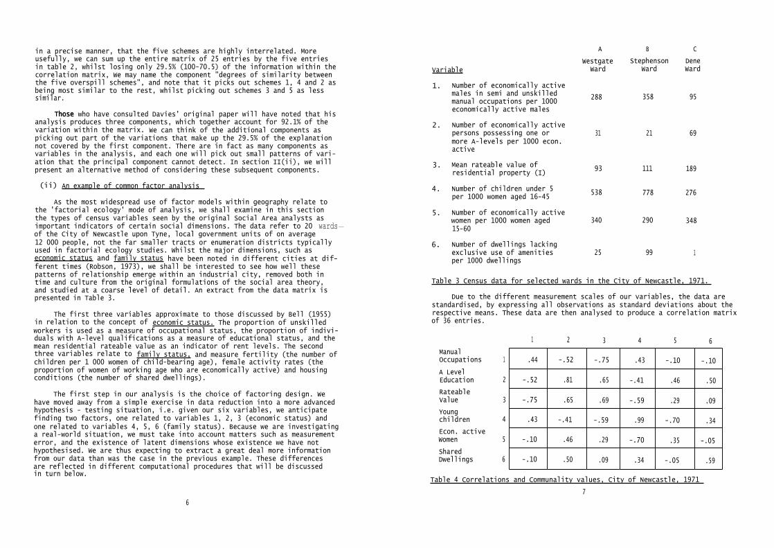
As the most widespread use of factor models within geography relate tothe 'factorial ecology' mode of analysis, we shall examine in this sectionthe types of census variables seen by the original Social Area analysts asimportant indicators of certain social dimensions. The data refer to 20 wards-of the City of Newcastle upon Tyne, local government units of on average12 000 people, not the far smaller tracts or enumeration districts typicallyused in factorial ecology studies. Whilst the major dimensions, such aseconomic status and family status have been noted in different cities at dif-ferent times (Robson, 1973), we shall be interested to see how well thesepatterns of relationship emerge within an industrial city, removed both intime and culture from the original formulations of the social area theory,and studied at a coarse level of detail. An extract from the data matrix ispresented in Table 3.

The first three variables approximate to those discussed by Bell (1955)in relation to the concept of economic status. The proportion of unskilledworkers is used as a measure of occupational status, the proportion of indivi-duals with A-level qualifications as a measure of educational status, and themean residential rateable value as an indicator of rent levels. The secondthree variables relate to family status, and measure fertility (the number ofchildren per 1 000 women of child-bearing age), female activity rates (theproportion of women of working age who are economically active) and housingconditions (the number of shared dwellings).

The first step in our analysis is the choice of factoring design. We have moved away from a simple exercise in data reduction into a more advancedhypothesis - testing situation, i.e. given our six variables, we anticipatefinding two factors, one related to variables 1, 2, 3 (economic status) andone related to variables 4, 5, 6 (family status). Because we are investigatinga real-world situation, we must take into account matters such as measurementerror, and the existence of latent dimensions whose existence we have nothypothesised. We are thus expecting to extract a great deal more informationfrom our data than was the case in the previous example. These differencesare reflected in different computational procedures that will be discussedin turn below.

Table 3 Census data for selected wards in the City of Newcastle, 1971.

Due to the different measurement scales of our variables, the data arestandardised, by expressing all observations as standard deviations about therespective means. These data are then analysed to produce a correlation matrixof 36 entries.

1 2 3 4 5 6

.44 -.52 -.75 .43 -.10 -.10

-.52 .81 .65 -.41 .46 .50

-.75 .65 .69 -.59 .29 .09

.43 -.41 -.59 .99 -.70 .34

-.10 .46 .29 -.70 .35 -.05

-.10 .50 .09 .34 -.05 .59

Table 4 Correlations and Communality values, City of Newcastle, 1971

7

ManualOccupations 1

A LevelEducation 2

RateableValue 3

Youngchildren 4

Econ. activeWomen 5

SharedDwellings 6

6

Fig. 2 Representation of data display in Fig. One.Fig. 1 Social variables in observation space. (Three Wards, (Scores in standard deviations)

City of Newcastle, 1971). (see text for explanation)

8 9

1

2

3

4

5

6

The major difference from the previous example is that the principaldiagonal of the matrix, i.e. the correlation of each variable with itself, r.--)does not contain values of 1.00. Instead we have inserted estimates of thevariation that each variable has in common with the other five variables, andwhich can be attributable to its correlation with one or more underlying com-mon factors. In factor analysis this is referred to as the communality. Thematrix shows that variables 1, 5, 6 have low communalities, and are perhapsaccounted for by a dimension, or dimensions, that we are not yet aware of.The methods used to determine the values of the communalities are discussedin Section IV.

The simplest way to understand the factoring procedure is to display thevariables and the resulting factors in a three-dimensional format (Figure 1).Here, the variables are located in object-space, i.e. each of the axes A, B,C represents one of our twenty wards; the location of the variables is withrespect to their value about the mean, represented by the darker, centralsphere. Further details of the physical model are provided in Kirby (1976).

Despite the small sample of wards, we can immediately see that a patternof relationships exists. To the left of the model, we can see a cluster,formed by variables 2, 3, 5 (education, rateable value and working women)whilst to the right we find variables 1, 4, 6 (occupation, fertility andshared dwellings). We may continue to define this pattern in a precise way,by examining the geometry of the interrelationships. Firstly, we may imaginea series of lines, usually termed vectors in this context, radiating out fromthe origin to the variables, like the spokes of a wheel about the hub. Thecloser the spokes, the more closely related are the respective variables. Wecan quantify this by measuring the acute angle between the 'spokes', and con-verting this to its cosine value. The cosine and the product moment correla-tion coefficient that we have already used are interchangeable, and in thisway we can determine the strength of relationship between our variables. Forexample, let us measure the acute angle 0 between the vectors connectingvariable 2, and variable 3, (Figure 2). This gives us a value of approxi-mately 100 : the cosine of this angle is in excess of 0.9. Consequently, wemay now state that the relationship between variables 2 and 3 is a correlationin excess of 0.9, i.e. strongly positive. If we return to table 3, we findthat the correlation value measured over all 20 wards is 0.65, again indicat-ing close relationship.

Rather than continue to measure a whole series of acute angles, betweenall the pairs of variables, we may summarise these inter-relationships withthe use of two further 'spokes', representing the resultants of the datavectors. Child (1970) suggests a useful analogy, whereby we may imagine theresultant of a series of vectors to be a generalisation of the divergentdirections in much the same way that the handle of a half-opened umbrella re-presents a middle way, or 'average' direction. These resultants are the factorsthat we are seeking, concisely stating the pattern of relationships withinthe vectors in the same way that we saw components summarising a correlationmatrix.

Figures 1 and 2 show the two factors in place. The factor running north-south is the principal factor. It can be seen that if the angles between thefactors and the original test vectors are measured as before, we can producethe correlation values, or loadings, between the variables and the factors.Thus, variables 2, 3 load most strongly on the first factor, as does variable

1 0

1, but with, of course, a different sign. Variables 4, 5, 6 are less highly

correlated.

The second factor normally displays less interesting patterns, in so faras the location is primarily determined by the first factor. It is typicalto find the second factor cutting across a swarm of data, producing a so-

called bipolar factor, where loadings are equally matched, positive-negative.In this example, variables 5, 6 both load quite strongly on this factor.

In a realistic research situation, we would not attempt to produce mean-ingful factors using only three cases, and for this reason we have not in-cluded in this section details of the loadings discussed above. Nevertheless,the general patterns found using these three cases are representative of theresults of the analysis using all the twenty wards. These are displayed inTable 5, in conjunction with detailed information on the interpretation offactor results.

Table 5 Output from factor analysis, City of Newcastle, 1971

11

As we noted above, the first factor is defined by positive associationwith the variables education, rent, and female labour and negatively by vari-ables indicating low social class and familism. The second factor is char-acterised by low loadings, except in the case of shared dwellings. An inter-pretation of these results suggests that whilst two dimensions of economicstatus and family status were hypothesised, we have here produced a generaldimension of social differentiation, picking out low social class and largefamilies on the one hand, and educational attainment, housing status andeconomically active women on the other. The variable measuring housing qual-ity appears to be unconnected with these other data items, loading as it doeshighly on the second factor. We may note that the existence of economicallyactive women has become an indicator of higher social status, as opposed tolower social status as hypothesised. Our interpretation of the second factor,which picks out shared dwellings, must rest to some degree upon our knowledgeof the city, for it seems likely that the scale of the analysis has failedto pick out the many pockets of shared dweIlings that exist in Newcastle, andwhich are closely related to the distribution of low economic status groupsand variations in rateable values. Such problems of interpreting, or labellingfactors, are very common.

To sum up this analysis, we must reject our hypothesis that two dimen-sions of urban differentiation exist. Whether this is a function of our database (i.e. Newcastle) or the scale of the analysis is a point that can onlybe determined by further analysis of other cities and of Newcastle, usingmore detailed data for enumeration districts. Attention must also be paid tothe fact that our level of explanation is quite low: the two factors consider-ed account for only 65% of the variation within the correlation matrix. Oncemore, we must suggest that further research is necessary to pin down whetherthis rather poor rate of explanation is due to the distortions of the scaleof the analysis, or the existence of latent dimensions of differentiationthat we have not hypothesised.

III PRACTICAL & TECHNICAL CONSIDERATIONS

(i) The route to a factor analysis

The two examples we have given suggest that in searching for orderthrough factor analysis we can attempt two separate although related tasks.First, we can eliminate the redundancies in the original set of data byattempting to summarise the variation in this set in terms of a smaller setof variables (or factors) which are a combination of the original variables.We then attempt to identify or name the underlying dimensions in the data setby examining the way in which the original variables have been combined inthe process of making this summary. The way we combine a set of characteris-tics such as occupation, education and income measured over a set of censustracts, may lead us to a basic underlying dimension that we might name "socialstatus". Each of the ariginal census tracts may be scaled along this dimen-;ion by computing its score on the basic factor. In more everyday language,we can combine many of the detailed characteristics of a number of motor carsto arrive at some underlying notion of "performance" and hence derive a multi-variate scale on which each individual car can be rated.

The second way in which we search for order amongst a set of phenomenais to postulate a limited number of variables or factors which are respon-sible for producing the inter-relations between the original variables. Forinstance, we could hypothesize that a force called "economic development"generates typical levels of G.N.P.,urban growth rates, levels of educationalattainment, etc. and test for the existence of such a basic dimension amongsta large set of variables measuring these characteristics.

In the first instance we have used factor analysis within an inductiveframework and in the second we have used it deductively. Usually factor analy-sis is regarded as a classical inductive method. Indeed, in most instancesit is used as an exploratory tool for unearthing the basic empirical regular-ities in a set of data. Used in this way, the technique is a very powerfuldescriptive device.

Methodological questions of induction and deduction are obviously notindependent of the problem under investigation. All of these matters closelyimpinge on the question of factor analysis research design. This is becausefactor analysis embodies a number of alternative procedures; indeed the term"factor analysis" should be regarded as a generic name for a family of multi-variate techniques. Any one problem might involve several of these procedures.Consequently the researchers will need to specify an appropriate factoringdesign. Figure 3 represents a flow diagram of a possible factor analysis re-search design. In many instances not all of the steps will necessarily beexecuted. The analysis may terminate at an early stage or certain steps maybe by-passed. Also, different methods of common factor analysis may be adopt-ed which do not involve all of the procedures suggested in Figure 3, whileother approaches provide statistical tests for the number of significantfactors. Although the diagram is not a completely general model of factoranalysis research design, it does cover the two most frequently used approachesin geography; it also provides a useful framework for the ensuring presenta-tion of issues.

Before proceeding one obvious point should be stressed: the variety ofalternative choices available at different stages in completing a factoranalysis means that each choice, or combination of choices, will produce adifferent end product. Although there are a number of guidelines as to themost appropriate choice at each stage, an element of subjectivity will in-evitably be involved. In many instances there may not be a single "right"answer. As the ultimate test of the success of the factor analaysis may be theinterpretability of the final results, producing an adequate factor analysisis as much an art as a science. However, one important scientific criterioncan be satisfied and that is reproducibility of the result by another investi-gator - provided that is, every choice that has been made is carefully docu-mented in writing up the results.

(ii) The Data Matrix

The first choice facing us concerns the selection of variables. The out-put of the factor analysis will obviously depend on the nature of the input.This is true of every statistical analysis, but because of factor analysis'sability to handle large numbers of variables there is a danger of this pointbeing overlooked. We may be tempted to include all of the variables available,for example in the census, without carefully considering the mix of under-lying dimensions that these variables cover. So it is not surprising that

13

12

Fig. 3 Routes to Factor Analysis. (*Possible termination points)

14

factor analyses of British cities often extract housing conditions as aprincipal factor underlying spatial variations in their internal structure,while in the American context an economic status dimension is usually moreimportant. This may simply reflect the fact that the British census containsmore indicators of housing conditions while the American census has moresocio-economic indicators. Having selected our variables we may be faced withthe question of the scale at which to carry out the analysis, that is, theselection of observations. For example, in a study of urban structure, shouldwe analyse the data at the level of the enumeration district (with an averagepopulation of 500) or wards (with an average population of 12 000)? The re-sults may differ significantly for these two scales.

The next step involves arraying the data in matrix form. Typically thiswould consist of n cases (census tracts, industrial plants, cities, etc.)over which m variables or characteristics are measured (Figure 4). These vari-ables may be measured in any units (dollars, people, tons, etc.) and scaledin any way (interval, ratio, nominal). It should be stressed that whereverpossible the number of cases (n) should exceed the number of variables (m).Re-examination of Figure 1 should immediately suggest the reason - namely thatthe observational space set up to contain the variables would have fewerdimensions than the number of variables. The position of any vector in thisspace could not therefore be uniquely determined. Such a matrix might be re-ferred to as a spatial structure matrix and form the initial data for a multi-factor uniform regionalisation (i.e. a grouping of the n cases on the basisof similarity in terms of less than m structural dimensions). Examples ofsuch matrices are provided by King's study of Canadian urban dimensions,where the observations consisted of 106 cities and the variables 50 socio-economic characteristics of these cities (King, 1966), and Goddard's studyof central London where the observations consisted of 260 city blocks and thevariables 80 different types of office employment (Goddard, 1968).

Fig. 4 Spatial structure and behaviour matrices

15

Alternatively, the new data matrix might consist of an n x m transactionmatrix in which the entries represent the flows between places (Fig. 4). Sucha matrix need not be symmetric (i.e. the flows from A to B may be greaterthan the flows from B to A). An example is given by Goddard's study of taxiflows in Central London (1970). Such matrices might be referred to as spatial behaviour matrices and form the initial data for a functional regionalisation(i.e. a grouping of places on the basis of functional ties).

Let us consider the structure matrix. Essentially two questions can beasked of the variation expressed in this matrix;

1. Which variables possess common patterns of variation over the setof observations? This is called R mode analysis (column-wisecomparisons)

2. Which cases possess similar profiles of scores over the set ofvariables? This is called Q mode analysis (row wise comparisons).

Whilst geographical literature has tended to concentrate upon the re-lationships between variables, it will be remembered that our introductoryexample was of relationships between observations: as Davies observes "onewould expect geographers to be more directly concerned with areal differencesand similarities" (Davies 1972, p. 115) and hence Q mode analysis. However,in many geographical studies the number of observations (areas) frequentlyexceeds the number of variables, thereby precluding Q mode analysis.

If the data matrix had been a cube with different time periods constitut-ing the third dimension, numerous other slices of the matrix could be takenfor analysis - for instance, where dates are the observations.

In the case of the transaction matrix, R mode analysis would comparedestinations in terms of similarities in the origin of the flows and Q modeanalysis would compare origins in terms of similarities in the destinationsof their flows.

(iii) Data Transformation

Having arrayed our raw data in matrix form, some transformations may berequired to take account of particular peculiarities of the data, such asdifferent measurement scales, or variations in the size of areal units. Forexample, it is common to express raw variables as ratios of some base popu-lation in an attempt to eliminate size effects. Thus to standardize for varia-tions between census tracts in the number of households we might express eachvariable as a ratio of the total number of households in the area (e.g. theproportion of households sharing a dwelling). If this were not done, thelargest amount of variation in the data could arise simply from differencesin the size of areal units, and this variation would be reflected in the firstfactor. However, in making such transformations we should be aware of twodangers. First, of false inferences that could be drawn from interpreting theresults in terms of the original and not the transformed variables, and second,of the danger of spurious correlation resulting from dividing a number ofvariables by a single common denominator. For example, the correlation betweenthe proportion of households renting their accommodation and the proportionowning their accommodation may be more strongly negative than that betweenthe absolute number of households in each category.

Some transformation of the data matrix may also be required by the fac-tor analysis method that is to be employed at a later stage. Data transform-ation may be divided into those that are applied to only single variables orsubsets of variables and those that are applied uniformly across the datamatrix.Distributional Transformations: It has commonly been assumed that factoranalysis requires the underlying distribution of the data to be of a multi-variate normal form; this implies that not only each variable is normally dis-tributed but that the relationship between all pairs of variables is linear.Some workers argue that normality is essential only if questions of statis-tical inference are involved. While this is true it should be stressed thata sufficient condition for the correlation coefficient (on which subsequentfactoring is based) to be a true measure of the statistical association be-tween two variables is that the bivariate distribution of the variables benormal. Therefore if product moment correlation coefficients are used as ameasure of spatial association between the m variables it is advisable thatthese variables be transformed such that the relationship between all pairsis linear. Transformation to normality for each variable will increase thechances of near linear relationships, but will not guarantee this.Matrix Transformations: If the data are measured in a large variety of dif-ferent units - for example some in terms of dollars, some in terms of popu-lation, some in percentages, it is necessary to standardise the data intosimilar units so that meaningful comparisons between the distributions can bemade. The most frequently used standardisation involves expressing the ori-ginal observations in standard score units. The standardisation transformationsubtracts the mean of the data for a variable from the original data and thendivides by the standard deviation. The effect of the transformation is to re-move the difference in mean and standard deviation between variables fromtheir co-variance; each variable now has a mean of zero and a variance of one.(Standardisation creates some problems as it generally gives equal weight toeach variable in the analysis, although some variables may be far more signi-ficant - in terms of exhibiting a wider range of variations over the set ofindividuals - than the others). The formula is:

(iv) The Correlation Matrix

Such a standardisation is effected when the product moment correlationsare computed between each of the variables in the data matrix. In the case ofa spatial structure data matrix the distributions of each pair of m variablesis compared over all of the observations to produce a symmetrical m x m cor-relation matrix. The correlation coefficients indicate similarities in theprofiles of each variable observed over the set of areal units. In the caseof the transaction matrix (R analysis), correlations between columns compareareas in terms of similarity in the profiles of their trip origins. No accountis taken of similarity in magnitude. In the analysis of transaction matricesit might be important to compare variables in terms of similarities in the

17

16

volume of, say, trade received. In this case, an alternative to the productmoment correlation coefficient, the pattern magnitude coefficient might beemployed; this takes account of both sources of variation. If, however, theflow matrix is symmetrical (i.e. flows from A to B equal those from B to A)raw data for each variable may be scaled to range from 0 to 1 and analysedas a correlation matrix (Rummel, 1970).

The type of coefficient employed in the transformation to a correlationmatrix will also depend upon the way in which the data is scaled. In the caseof nominal data the phi coefficient may be employed: a recent example of theanalysis of binary data is provided by Tinkler (1972,1975) & Hay (1975). Inthe case of ordinal data some rank order coefficient and in the case of scaledata (i.e. data with a restricted range) some non-parametric coefficent shouldbe applied. Any of the matrices of coefficents may be factored. Alternatively,and this is particularly relevant in the case of transaction matrices, theraw data may be directly factored without computing the correlation coeffic-ients. (Horst, 1965, Russett, 1967).

Much useful information can be gained from careful examination of thecorrelation matrix. Identification of clusters of highly inter-correlatedvariables can sometimes provide a guide as to the number and character of theunderlying common factors. All too often in geographical studies no attentionis given to the correlation matrix.

IV THE FACTOR MODEL

In the introductory sections we touched upon the differences that existbetween principal components analysis and common factor analysis. The twoexamples discussed have provided an example of each model. We shall now con-trast the two forms of analysis in greater depth.

(i) Principal Components Analysis

Principal components analysis is a data transformation procedure appliedto the raw data matrix Z. Essentially it seeks to replace the m columns of Zwith new columns, which, if represented geometrically as vectors, would bemutually orthogonal. We seek to define a new set of variables or componentsthat are uncorrelated and where the definition of these components is in termsof m coefficients relating them to the original variables.

A geometric interpretation for two variables is possible. Consider aconventional scatter diagram in which the co-ordinate axes represent the twovariables Z 1 and Z 2 and the location of the observations are defined by theirscores on each of these variables (Fig. 5). Notice we have defined a variable space and not an observational space as in Fig. 1. The oval shape of theswarm of points is indicative of the correlation between the two variables.A perfect circle would indicate zero correlation; in fact we could rotate thevariable axes to such a position that the points were in a circular swarmand the angle between these axes would again indicate the degree of correla-tion. The two representations can therefore be transformed into one another.

Fig. 5 Components as the major and minor axes of an elipse

1819

so that it lies along the principal axis

21

The above procedure can be readily extended to more than the two dimen-sions.The following properties hold:-

1. The first component always accounts for the greatest amountof variance in the original scatter of points.

2. When the number of variables is greater than two then thesecond component accounts for the greatest proportion ofresidual variance (i.e. that remaining after that due tothe first component is removed).

3. There are exactly the same number of components as originalvariables and the components are ordered in terms of theproportion of variation in the original data set accountedfor by each component.

4. In cases in which the number of variables is large thegreat majority of the variance in Z is accounted for bya relatively small number of components. This achieves aparsimonious description of the data.

The principal axes of a data matrix can be conveniently solved foralgebraically. The question is what transformation will rotate the variableaxes so that they lie co-linear with the principle axis. These transformationsare provided for by solving for the eigen-values and the associated eigen-vectors of the full correlation matrix (i.e. with "ones" in the diagonal;1.0 equals the variance of each standardised variable. Thus the total amountof variance to be accounted for is equal to the sum of the diagonal elementsof the correlation matrix). The eigen-value indicates the length of each ofthe axes, i.e. the amount of common variance accounted for by each axis.Gould has provided a useful geographical interpretation of eigen-values(Gould, 1967). Dividing the eigen-value by the number of variables indicatesthe Proportion of the total variance in the standardised data matrix account-ed for by each component. By scaling each eigen-vector by its associatedeigen-value we reduce the length of the eigen-vector proportional to thelength of the principal axis it measures. The elements of the eigen-vectorscontain the transformation coefficients for the variables that rotates eachvariable axis by the angles(Fig. 6).

These coefficients are the correlations or loadings of each variable onthe successive principal axes. With m variables there will be m eigen-valuesand associated vectors. The first will account for the largest amount ofvariance in the standardised data matrix, the second the largest amount ofvariance in the residual matrix after the first eigen-value has been extracted,and 50 on. Together the m values will account for the total amounts of vari-ance in the original data. It is thus possible to write a series of equations,one for each variable, to completely specify or recreate the original vari-

20

Examinations of the coefficients in these equations (the component load-ings or the correlations between the component and the variable) helps in thenaming of the component.

Components analysis alone is most useful when there is a major dimensioof variation in a data set which itself identifies a clearly discernible concept and within which there are no important sub-concepts. Berry, for instan e,has used each country's score in a cross national components analysis ofsocio-economic variables to place it on a multi-variate scale of economicdevelopment (Berry, 1960). Similarly, Gould in several studies has used com-ponents analysis to extract the group image in studies of residential prefeences. (For example, Gould and White, 1968). From an n place x m individualmatrix of preference scores, he extracts the principal components which usually accounts for a substantial proportion of the original variance. Mappingof components scores for the n places reveals the group's common preferencsurface.

A further important use of principal components analysis is as a straight-forward data transformation to meet the assumptions of other techniques. Inparticular multiple regression assumes that the predictor-variables, the so-called independent variables, are uncorrelated. If the independent variablesdisplay strong inter-correlations then components analysis can be applied toorthogonalise the data; if sufficient variance is explained the scores of theobservations on the leading component can be entered into a simple regressionin lieu of the original intercorrelated variables. If interpretation is notpossible or if explained variance is low, the scores from more than one com-ponent can be entered in a multiple regression. An example is provided byBritton's gravity model study of the freight hinterland of Bristol whereseveral mass factors were highly inter-correlated and had to be transformedin a principal components analysis before calibrating the model through mul-tiple regression. ( Britton, 1968).

It should be stressed that principal components analysis is essentiallyvariance orientated. If we return to the geometric interpretation, a con-figuration of m variables will describe a hyperelipsoid in m dimensions (inthree dimensions a rugby football provides a good analogy of the shape). Thefirst component will be inserted along the principal axis of variation re-gardless of the existence of distinctive clusters of variables in this space.All variables included in the analysis, no matter how randomly they are re-lated to the rest of the data set, would influence this principal axis ofvariation. Most variables will therefore load fairly high on this component.In many geographical studies, when the data has not been weighted for differ-ences in the sizes of areal units, this first component can often be identi-fied as a size factor. The second component will be inserted orthogonally tothe first and will often be bi olar, i.e., with both high negative and posi-tive loadings, which creates di iculties in interpretation. (i.e. in the dis-tinguishing of independent clusters of variables)

If interpretation of the underlying dimensions is sought, rather thansimple parsimonious description of the data, two other procedures presentthemselves. First, rotation of the principal axes to some more meaningfulposition that better describes the initial clusters of variables, and second-ly, the adoption of a fundamentally different factoring technique, namelycommon factor analysis, which concentrates on the major patterns of variationand chooses to ignore the remainder.

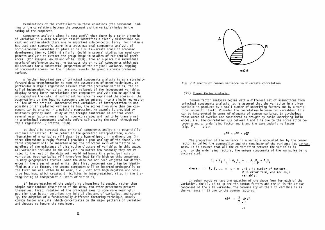
Fig. 7 Elements of common variance in bivariate correlation

(ii) Common Factor Analysis

Common factor analysis begins with a different set of assumptions fromprincipal components analysis. It is assumed that the variation in a givenvariable is produced by a small number of underlying factors and by a varia-tion unique to itself. Consider the correlation between two variables: thiscan be interpreted in terms of elements of common variance. In psychologythose areas of overlap are considered as brought by basic underlying influ-ences, i.e. the correlation (r) between A and B is due to the correlation be-tween A and an underlying factor and B and the same underlying factor(Fig. 7). Viz:-

The proportion of the variance in a variable accounted for by the commonfactor is called the communality and the remainder of the variance its unique-ness. It is assumed that all the co-variation between the variables ispro by the underlying factors, the unique components of the variables beinguncorrelated:

In other words we have one equation of the above form for each of thevariables, the Fl, F2 to Fp are the common factors and the Ui is the uniquecomponent of the i th variable. The communality of the i th variable hi isthe variance in Zi due to the common factors:

23

22

The uniqueness of the i th variable is equal to 1 minus its communality.Provided that the factors are orthogonal, the coefficients Aik still representthe correlation between the i th variable and the k th factor.

The use of this model poses two problems. First one does not initiallyknow the magnitude of the unique components of variation for each variableand hence its communality. And second, one does not know the number of commonfactors which are appropriate. In psychology the number of basic dimensionscan often be hypothesised from theory but in most goegraphic applicationsthis is rarely the case.

(iii) Communality

Standard procedures have now been developed for estimating initial com-munalities and comparing these with final communalities and reiterating theprocess until there is no significant change. The lower bound for this esti-mate has been shown to be provided by the square of multiple correlation re-sulting from the regression of the m th variable on all the other m - 1 vari-ables. The communality estimates are inserted in the diagonal of the cor-relation matrix. We are thus assuming that the variance of a variable to beexplained by the common factors is less than 100%. The analysis is pursuedin the same way as that outlined for principal components analysis. Finalcommunalities (i.e. the actual amount of variance explained by each of thecomponents) are reinserted in the diagonal of the correlation matrix and theprocesses reiterated until some satisfactory convergence is achieved.

(iv) The number of factors

Using the principal axes method, factors are extracted successively -the first accounting for the maximum amount of variation; the second axis isthen extracted from the residual correlation matrix and so on. The questionthen arises as to when to stop extracting eigen-vectors. Several rules ofthumb have been suggested as to the number of factors, but the ultimate testis the interpretability of the resulting factors. One may initially opt fora satisfactory amount of explained variance and this is usually provided byall those eigen-vectors with eigen-values greater than 1.0 - i.e. only thosefactors that account for more than their proportionate share of the originalvariance. Within these limits a rough guide to interpretability is providedby plotting factors against eigen-values and seeking a distinct break ofslope (Fig. 8). Figure 8 provides one such "scree diagram" from a studywhich sought to identify the number of distinct spatial clusters of officeactivities in the City of London (Goddard 1968). It will be seen that beyondthe sixth component each additional component accounts for approximatelysimilar and trivial amounts of variance.

(v) The Rotation of Factors

In some investigations we may only be concerned with obtaining a parsi-monious description of our data while in other instances we may aim to ident-ify distinctive clusters of variables. If the latter is our aim it may benecessary to carry out a rotation of the original factors; this is becausethe initial solution will identify the principal patterns of variation andnot necessarily distinctive clusters of variables.

Fig. 8 Trivial and non-trivial eigenvalues. (Source: Goddard, 1968)

Fig. 9 Orthogonal rotation of overspill data. (dashed lines, loadings onprincipal components, dotted lines, loadings on Varimax rotated com-ponents, V.1 and V.II) (Source: Davies, 1971)

2524

PRINCIPAL COMPONENT SETA. Unrotated component loadings

I

Component

III

Pattern of highloadings

II I II III

Aldridge 1 0.93 -0.16 -0.26 *Scheme

2 0.83 -0.23 -0.23 *

3 0.77 -0.45 -0.13 * *

Macclesfield 4 0.86 0.36 0.13 *Scheme

5 0.81 0.46 0.46 * *

B. Varimax rotated component loadings

I

Component

III

Pattern of highloadings

II I II III

Aldridge 1 0.89 0.34 0.15 *Scheme

2 0.85 0.28 0.08 *

3 0.87 0.16 -0.15 *

MacclesfieldScheme 4 0.36 0.91 0.04 *

5 0.21 0.99 -0.01 *

Table 6: Unrotated and rotated component loadings: housing schemes in Aldridge and Macclesfield (Source Davies, 1971)

Re-examination of the original example of overspill schemes in the twotowns will illustrate this point. It will be recalled that one component wasextracted that was labelled the degree of similarity" between the twoschemes. A second component could be extracted on which schemes 1, 2 and 3had low negative loadings and schemes 4 and 5 low positive loadings (Table 6).Such a component is referred to as bipolar and is often difficult to inter-pret. However, if we rotate the original components about their origin two"new" components can be identified in which schemes 1, 2 and 3 load highlyon factor 1 and schemes 4 and 5 on factor 2 (Figure 9 and Table 6). Therotation is performed without changing the position of the original variables;the co-ordinate axes are merely transformed. In this example the uncorrelated(or orthogonal) characteristics of the original components are also preserved.

Fig. 10 Principal components and rotated factor subsets

In carrying out this rotation the general concept of the degree of similar-ity between the overspill scheme has been broken down into two more specificsub-concepts which in this case separate out the overspill schemes in thetowns into two distinctive classes. Figure 10 attempts to summarise thispoint in the form of a Venn diagram.

Whether such a breakdown of the generality of a principal component isdesirable depends entirely on the purpose of the investigation. In the studyof overspill schemes the requirement was for a general index of similarity.In another study aimed at a functional regionalisation of Central London onthe basis of data on inter-zonal taxi flows specificity was the objective(Goddard 1970). The principal component simply identified those zones thatwere linked by large volumes of traffic; analytic rotation divided these intotwo meaningful functional sub-regions. In so doing some of the variance assoc-iated with the principal component was redistributed between other components.This is illustrated in Table 7.

The usual criterion for rotation is that of simple structure, namelythat each variable loads highly on one and only one factor, (Table 8).This can be achieved by the use of a number of algebraic (as opposed tographical) criteria of which the most widely adopted is referred to as the"normal varimax criterion". As the name implies this seeks to maximise thevariance of the loadings on each factor, that is to achieve as many high andas many low loadings as possible.

Using the varimax criteria the orthogonality of the original factors ismaintained. However, in reality we might expect that the basic factors under-lying the observed intercorrelation amongst our original variables may them-selves be intercorrelated. For example, in the studies of the factorial ecology of a city it would be reasonable to assume that a factor describing theeconomic status of areas may be related to another describing their familystatus. This consideration led Bell to attempt to achieve a more meaningfuldescription of urban spatial structure using an oblique rotation of an initialfactor analysis. (Bell, 1955). The result of an application of an obliquerotation procedure to the analysis of social economic data for the Newcastlewards is described in Table 9 and Figure 11. From this analysis it will beseen that there is indeed a small correlation between the two factors original-ly identified (R = -0.12). It will also be seen that this rotation does bring

2726

Component I II III IV V VI Total

Eigenvalue 18.0 7.2 4.8 4.4 3.9 2.9

% explanation 26.0 10.5 7.0 6.3 5.6 4.2 59.7

Rotated component I II III IV V VI Total

Sum of squaredloadings 10.8 8.3 6.9 6.0 5.4 3.8% explanation 15.7 12.0 9.9 8.7 7.9 5.6 59.7

Table 7: Explained variation associated with rotated and unrotated component analysis (Source: Goddard, 1970)

Variables I

Unrotated

Variables

Simple StructureFactors Factors

IIIII III I II

1 * * 1 *

2 * * * 2 *

3 * * * 3 * *

4 * * 4 *

5 * * * 5 *

6 * * 6 * *

7 * * 7 *

* Indicates a high factor loading.

Table 8: Hypothetical example of simple structure

us closer to the ideal of simple structure. Oblique factor 1 is more clearlyidentified as a social class factor and oblique factor 2 as a family statusfactor. This is principally because the rotation has succeeded in reducingthe loadings of variable 4 (number of children under 5) and variable 5(economically active women) on factor 1 and increasing them on factor 2,although the signs of the loadings of the two variables on factor 2 are ob- ,4viously different.

Oblique rotation is conceptually attractive because in theory it can beshown to be the more general case; if the original clusters of variables areindeed orthogonal, an oblique rotation procedure should identify uncorrelatedfactors. Furthermore, with oblique rotation it is possible to carry out ahigher order factor analysis of the correlations between the oblique factorsthemselves, thereby identifying more general underlying dimensions - althoughthere is a danger here of reproducing one's original (general) principalfactor.

28

Fig. 11 Oblique rotation of social variables, City of Newcastle, 1971.(dashed lines, structure loadings, dotted line, pattern loadings).

Against these advantages there are a number of analytical problems. Un-like orthogonal rotation, there can be no unique solution; while algebraicprocedures are available the degree of obliqueness permitted is a matter forthe investigator to specify. Also, once orthogonality is relaxed, the 1 to 1correspondence between factor loadings and correlation coefficients is lost.Re-examination of figure 11 will reveal that in fact two sets of "loadings"can be identified. Those that are given in their entirety are the correlationsbetween the variables and the factors since they are perpendicular projectionsof the variables onto the oblique factors. These are referred to as structure loadings. However, a second set of loadings, referred to as pattern loadings,could be derived; in the case of pattern loadings on oblique factor 1 theseprojections would lie parallel to oblique factor 2. For clarity, only onesuch pattern loading is shown on Figure 11.

A further complication is that a second set of underlying reference axes at right angles to the primary oblique factors can be constructed and a fur-ther set of pattern and structure loadings calculated. The primary referenceaxes are sometimes the most appropriate for delimiting simple structure.

29

Variable

1. Manual

I

Unrotated Oblique rotated

II I II

occupation -0.65 -0.14 0.66 -0.13

2. A leveleducation 0.79 0.42 -0.88 -0.06

3. Rateablevalue 0.82 0.09 -0.81 0.25

4. Youngchildren -0.81 0.57 0.60 -0.88

5. Econ. activewomen 0.53 -0.25 -0.43 0.46

6. Shareddwellings 0.11 0.76 -0.33 -0.67

(r -0.12)

Note: No sigificance is attached to the reversal of signs of variablesbetween the rotated and unrotated solutions if the relationshipof variables one to another within a factor remains unaltered(i.e. -, +, +, -, +, + has the same interpretation as +, -, -,

+, -,-).

Table 9 Unrotated and oblique rotation of social variables, City of Newcastle, 1971.

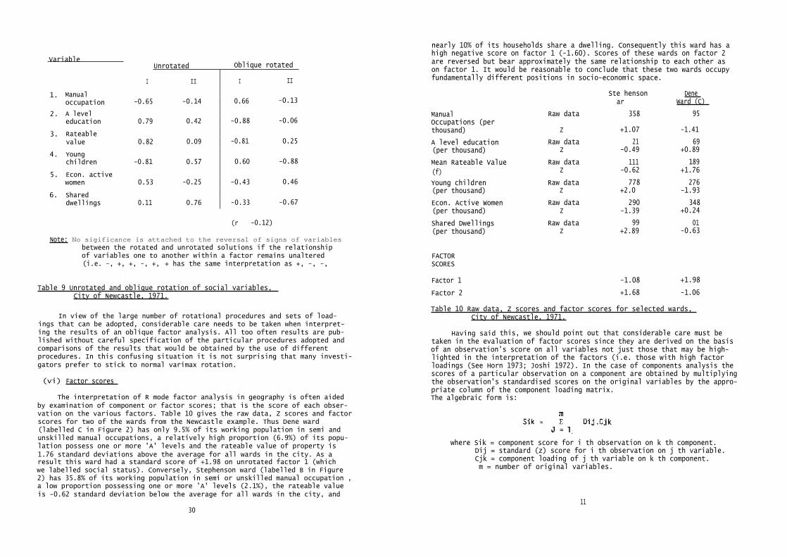
In view of the large number of rotational procedures and sets of load-ings that can be adopted, considerable care needs to be taken when interpret-ing the results of an oblique factor analysis. All too often results are pub-lished without careful specification of the particular procedures adopted andcomparisons of the results that would be obtained by the use of differentprocedures. In this confusing situation it is not surprising that many investi-gators prefer to stick to normal varimax rotation.

(vi) Factor scores

The interpretation of R mode factor analysis in geography is often aidedby examination of component or factor scores; that is the score of each obser-vation on the various factors. Table 10 gives the raw data, Z scores and factorscores for two of the wards from the Newcastle example. Thus Dene ward(labelled C in Figure 2) has only 9.5% of its working population in semi andunskilled manual occupations, a relatively high proportion (6.9%) of its popu-lation possess one or more 'A' levels and the rateable value of property is1.76 standard deviations above the average for all wards in the city. As aresult this ward had a standard score of +1.98 on unrotated factor 1 (whichwe labelled social status). Conversely, Stephenson ward (labelled B in Figure2) has 35.8% of its working population in semi or unskilled manual occupation ,a low proportion possessing one or more 'A' levels (2.1%), the rateable valueis -0.62 standard deviation below the average for all wards in the city, and

nearly 10% of its households share a dwelling. Consequently this ward has ahigh negative score on factor 1 (-1.60). Scores of these wards on factor 2are reversed but bear approximately the same relationship to each other ason factor 1. It would be reasonable to conclude that these two wards occupyfundamentally different positions in socio-economic space.

Ste henson Dene ar Ward (C)

Manual Raw data 358 95Occupations (perthousand) Z +1.07 -1.41

A level education Raw data 21 69(per thousand) Z -0.49 +0.89

Mean Rateable Value Raw data 111 189

(f) Z -0.62 +1.76

Young children Raw data 778 276(per thousand) Z +2.0 -1.93

Econ. Active Women Raw data 290 348(per thousand) Z -1.39 +0.24

Shared Dwellings Raw data 99 01(per thousand) Z +2.89 -0.63

FACTORSCORES

Factor 1 -1.08 +1.98

Factor 2 +1.68 -1.06

Table 10 Raw data, Z scores and factor scores for selected wards, City of Newcastle, 1971.

Having said this, we should point out that considerable care must betaken in the evaluation of factor scores since they are derived on the basisof an observation's score on all variables not just those that may be high-lighted in the interpretation of the factors (i.e. those with high factorloadings (See Horn 1973; Joshi 1972). In the case of components analysis thescores of a particular observation on a component are obtained by multiplyingthe observation's standardised scores on the original variables by the appro-priate column of the component loading matrix.The algebraic form is:

where Sik = component score for i th observation on k th component.Dij = standard (z) score for i th observation on j th variable.Cjk = component loading of j th variable on k th component.m = number of original variables.

1130

From this equation it should be clear that each score is the sum of aseries of small products and that similar final sums can be arrived at in avariety of ways. Horn gives a simple example to illustrate this point:

The implication is that observations with similar component scores willnot necessarily have the same profile in terms of the raw variables. Thispoint should be borne in mind when using component scores as the basis forsampling areas for more detailed investigation. The simple message, as withall statistical techniques, is that careful examination of the raw data shouldbe a prelude to more advanced analysis.

A final warning before leaving this subject. In components analysis allof the variation in the original variables is accounted for by the componentsso we can therefore completely recreate our original observation in terms ofour newly derived components simply by carrying out the simple matrix multipli-cation that we have described. However, in factor analysis, where there issome residual or unexplained variation, we have to estimate the scores of eachobservation on the factors. These estimates are obtained by the use of multipleregression techniques.

V SOME GEOGRAPHICAL EXAMPLES OF FACTOR ANALYSIS

In sections 1 and 2 we attempted to contrast two approaches to factoranalysis, namely an inductive (descriptive) approach and a deductive (hypo-thesis-testing) approach. These are probably over-pompous terms for what mayseem in the end to be two rather descriptive pieces of work. Nevertheless,the perspectives adopted were somewhat different. Rummel has suggested a ten-fold classification of the types of research strategy within which factoranalysis techniques may be employed (Rummel 1970). In this section we shallattempt to illustrate this classification by drawing upon examples from thegeographical literature (Table 11). Our aim in doing this is merely to sugges

tithe range of contexts in which factor analysis has been utilised in geographyWe appreciate that other authors might have selected different examples orcategorised the ones that we have taken differently. We hope that readers wilfollow up the examples' for themselves if only to see whether they agree withour classification!

The first illustration considers inter-relationships within a data set,where there exist a number of covariant variables. The examples chosen arethe overspill schemes discussed by Davies in section 1, where we were ableto express the original correlation matrix in terms of two components, whilstlosing only a small amount of the information within the data.

32

Table 11 A classification of factor analysis research strategies illustratedby geographical examples.

Strategy Example Subject Data

Inter-relationship Davies (1971) Overspill schemes 59 questionnaireitems, 5 over-spill schemes.

Parsimony Moser & Scott(1961)

Classification ofBritish towns

60 census vari-ables for 1951.

Structure Sweetser(1969)

Comparison ofecological struc-ture in Boston &Helsinki

Census data.34 variables.

Classification Davies (1972(a))

Analyses of flowdata to defineregional & func-tional structure

Shopping trips.108 settlements& 40 centres,S. Wales.

Scaling Robson (1969) Creation oftaxonomic unitswithin which toassess educationalachievements, etc.

Census data, 30variables forSunderland.

Hypothesis-Testing Bell (1955) Creation of dimen-sions of socialstructure tojustify hypothesis.

Seven censusvariables forL.A. 570 censusunits

Data-Transformation Kirby &Taylor (1976)

Creation oforthogonal regres-sion inputs inreferendum analysis

Eight variablesfor 23 G.B.regions.

Exploratory Goddard(1970)

Study of taxi flowswithin London toidentify functionalregions.

Taxi flows withinLondon.

Mapping Rees (1970) Examination ofsocial space inChicago.

57 censusvariables.

Theory Openshaw(1973 (B))

Rotation by cri-teria of pre-determined spatialpatterns of factorscores

Morphologicaldata,S. Shields.

33

The second category relates to parsimony, or the reduction of a largenumber or variables to manageable proportions. One of the best examples isprovided by Moser & Scott (1961), who classified 157 British towns in re-lation to 60 census variables. Naturally, a classification based upon fourfactors, rather than 60 variables, is both speedier and more meaningful.

At this point we should emphasise that factor analysis will not producea classification of our observations in the strict sense of assigning themto discrete classes. For this we need to revert to some grouping algorithm.One of the reasons Moser & Scott sought to reduce their number of variableswas that they had no such algorithm available and were forced to subjectivelygroup British towns on the basis of common patterns of scores on the factors.Despite this, Moser & Scott's study remains as one of pioneer uses of factoranalysis in the social sciences.

Rummel defines structure in terms of analysis of the common elementswithin different samples. An interesting example of this is provided bySweetser (1969), who performed a factorial ecology on data for both Bostonand Helsinki. Whilst socio-economic status and family status were of similarimportance in both cities, Sweetser noted that unique dimensions of careerwomen (Helsinki) and ethnicity (Boston) existed.

The fourth category relates to the widest use of factor methods, notablythe creation of weighted scales by which to score the base units, in orderto create like regions. This strategy has been employed numerous times in theexamination of factorial ecologies of many cities, (for a full bibliographysee Robson (1973)). One of the earliest and most detailed studies was under-taken by Robson (1969). Here, a principal components analysis was undertakenupon 30 census variables, each measuring some aspect of economic structureor housing type for each of 263 enumeration districts in Sunderland. Fourdimensions resulted, which measured social class, housing quality, tenure anda generalised poverty factor. Each component was multiplied by the originaldata to give component scores, which were then combined into homogenous groupsusing cluster analysis. These in turn became the new base units for a studyof attitudes to education within the city.

Davies provides another example of factor analysis, with his study ofshopping trips (Davies 1972(a)), which we use to illustrate a classificatory strategy. Here, a Q-mode analysis (using places for variables within theinitial data matrix) was undertaken upon the flows between 108 settlementsand 40 shopping centres in South Wales. The resulting ten components pickedout the settlements with similar flow patterns, whilst the scores showed thepatterns of spatial association between centres and settlements. These patternsof shopping trips were then used to define functional regions for furtheranalysis. It is to be noted that although both Robson and Davies used factormethods to create taxonomic units, their methods were rather different.Robson's research involved two stages: the creation of scales (the components)which measured aspects of social differentiation, and the mapping of thescores of areas on these scales. Davies, by way of contrast, had a finitedata set of observations, and the problems of choosing meaningful census vari-ables, or interpreting (or rejecting) factors did not arise.

We take as our example of hypothesis-testing the work of Bell (1955)that we have already considered in section (ii). It remains one of the clear-est examples of quantitative analysis being used to test an a priori (orpreviously developed) hypothesis.

34

The seventh category derived by Rummel is that of data transformation.A simple example is provided by Kirby & Taylor (1976). Here, the authorsattempted to explain the variation of the 1975 E.E.C. Referendum vote in 23regions of the U.K., in terms of one (or both) of the following hypotheses:namely that the vote was a result of normal political cleavages, or a loca-tional factor, whereby distance from government produced an alienation effect.Eight variables were chosen to represent shades of these hypotheses, and afactor analysis undertaken to produce two (uncorrelated) varimax factors.The rotation was necessary to satisfy the requirements of the linear regres-sion model, by which the voting data was compared with the locational factor,and the political factor scores. The regression results indicated that thelocational factor could be removed from the analysis.

The category of exploratory use relates to areas in which little workhas been undertaken, and where the researcher has no opportunity to undertakecontrolled laboratory experiments, a situation which is normally the case insocial science. The example chosen here is Goddard's 1970 study of taxi flowswithin London, which was a preliminary to investigating the functional struc-ture of a metropolitan centre. Once more, the analysis is similar to thatundertaken by Davies, in so far as classification is a final step.

The term mapping may cause some confusion in the geographic context.Rummel's term relates to the reworking of known empirical concepts in differentsituations in an attempt to discover sources of variation and common elements.Again, factorial ecologies are the widest example of this approach, whilstRees' study of Chicago is perhaps the most detailed published examination ofthe social space of a major city.

The concluding section concerns the use of factor methods in a theoretical context, i.e. utilising the linear algebra within the model to make rigorousmathematised deductions about the data under analysis. Such high levels ofresearch are rare in geographical analysis, and one of the very few examplesis provided by Openshaw (1973(B)). Openshaw has been concerned with the effectsof scale on relationships, a fundamental concept elaborated by Blalock (1964),and the effects of autocorrelation within data, an equally fundamental consid-eration, discussed fully by Cliff & Ord (1973). These interests have led himto argue that it is possible to rotate factors to situations in which thespatial autocorrelation of factor scores is at an extreme,thereby providinginformation concerning the relationships between the variables, and theirspatial patterns. He has also performed factor analyses using data from dif-ferent size lattices, and examined the resulting variations in loadings andeigenvalues (Openshaw 1973(a)).

It is to be noted that these examples have several similar elements, andindeed, Rummel's classification could easily be compressed, or extended.Nevertheless, the sheer scope of the technique underlines the importance ofour interest in factor methods.

35

VI CONCLUDING REMARKS

This monograph can only serve as an introduction to factor analysis.We are conscious of the fact that we have only discussed two members of thefactor analysis family, namely principal components analysis and common fac-tor analysis, and that there is a rapidly widening range of solutions, suchas image analysis and alpha analysis, many of which bypass some of themethodological difficulties that we have touched upon. We have also avoideddiscussing in any detail the various analytical rotation procedures that gounder such glorious names as "oblimin" and "biquartimin". But these are allissues to be taken up in a more advanced monograph. All we have attempted isto describe "old-fashioned" factor analysis as it has been used and stillcontinues to be used in geography.

"Fashion" is a good note to conclude on. Factor analysis has been verymuch in fashion amongst geographers, but many of those who leaped onto thebandwagon in the early days have now jumped off. Those who remain see factoranalysis as a useful tool in certain contexts, to be taken up after only care-fully exhausting what can be gained from the data by simpler forms of analysis.Perhaps one of the reasons why factor analysis is likely to remain an attrac-tive tool for some geographers is the fact that it seldom produces "right"answers; a great deal of intuition and a large number of computer runs areusually needed to produce a "satisfactory" result (if we are honest, mostwould agree that research in fact progresses in this way).

Our final stricture will either make the reader a factor analyst forlife or cause him or her to abandon the technique for ever. This is to grabsome census data for your town, a factor analysis program and a large computerand run the data through the program ten, twenty, maybe thirty times, tryingall of the options. But be warned: Most computer centres are rationing com-puter paper these days.

36

REFERENCES CITED WITHIN THE TEXT

Bell, W. (1955), Economic, family and ethnic status: an empirical test.American Sociological Review, 20, pp 45-52.

Berry, B.J.L. (1960), An inductive approach to the regionalization ofeconomic development and cultural change. in: Essays on geography& economic development, (ed) N. Ginsberg, (Research Paper 62,Department of Geography, University of Chicago).

Berry, B.J.L. & Horton, F.E. (1970), Geographical perspectives on urbansystems. Englewood Cliffs.

Blalock, H.M., Jr. (1964), Causal inferences in non-experimentalresearch. University of North Carolina Press, Chapel Hill.

Britton, J.N.M. (1968), Regional analysis & economic geography - Acase study of the Bristol Region. G. Bell & Sons, London.

Child, D. (1970), The essentials of factor analysis. Holt, Rinehart &Winston.

Clark, D. (1975), Understanding canonical correlation analysis. CATMOG, 3,(Geo-Abstracts Ltd)

Cliff, A.D. & Ord, K. (1973), Spatial autocorrelation. Pion Press.

Davies, W.K.D. (1971), Varimax and the destruction of generality - a methodo-logical note. Area, 3, pp 112-8.

Davies, W.K.D. (1972), Conurbation and city region in an administrativeborderland; a case study of the greater Swansea area. RegionalStudies, 6, pp 217-36.

Goddard, J.B. (1968), Multivariate analysis of office location patterns inthe city centre: a London example. Regional Studies, 2, pp 69-85.

(1970), Functional regions within the city centre: a study by factoranalysis of taxi flows in central London. Transactions Instituteof British Geographers, 49, pp 161-182.

Gould, P.R. (1967), On the geographic interpretation of eigenvalues.Transactions Institute of British Geographers, 42,pp 53-86.

Gould, P.R. & White, R.R.(1968), The mental maps of British school leavers.Regional Studies, 2, pp 161-182.

Gregory, S. (1963), Statistical methods & the geographer. Longmans,London.

Harman, H.H. (1960), Modern factor analysis. University of Chicago Press.

Hay, A. (1975), On the choice of methods in the factor analysis of connect-ivity matrices - a comment. Transactions Institute of BritishGeographers, 66, pp 163-167.

Horn, C.J. (1973), Factor scores and geographical research. Institute ofBritish Geographers, Quantitative Methods Study Group,Working Paper I, pp 26-29.

Horst, P. (1965), Factor analysis of data matrices. Holt, Rinehart &Winston.

37

Joshi, T.R. (1972), Towards computing factor scores.in: Internationalgeography, (ed) W.P. Adams & F.M. Helleiner, (Montreal I.G.U.)

King, L.J. (1969), Cross-sectional analysis of Canadian urban dimensions,1951 and 1961. Canadian Geographer, 10, pp 205-224.

Kirby, A.M. (1976), A three-dimensional model for the introductory teachingof multivariate analysis. International Journal of Mathe-matical Education in Science & Technology. (forthcoming)

Kirby, A.M. & Taylor, P.J. (1976), A geographical analysis of the votingpattern in the E.E.C. referendum June 5, 1975. Regional Studies,(forthcoming).

Knox, P.L. (1974), Spatial variations in levels of living in England andWales in 1961. Transactions Institute of British Geographers62, pp 1-24.

Moser, C.A. & Scott, W. (1961), British towns: a statistical study oftheir social and economic differences. Oliver & Boyd.

Openshaw, S. (1973 a), An empirical study of the influence of scale onprincipal component and factorial studies of spatial association.Paper presented to Institute of British Geographers, January, 1973.

Openshaw, S. (1973 b), Some ideas concerning a spatial criterion for geo-graphical factor analysis. Paper presented to Institute of BritishGeographers, August, 1973.

Rees, P.H. (1970), The factorial ecology of Chicago. in: op. cit, (ed)B.J.L. Berry & F.E. Horton.

Robson, B.T. (1969), Urban analysis: a study of city structure withspecial reference to Sunderland. Cambridge University Press.

(1973), A view on the urban scene. in:studies in human geo-graphy, (eds) M.K. Chisholm & B. Rodgers, Heinemann.

Rummel, R.J. (1970), Applied factor analysis. Northwestern UniversityPress.

Russett, B.M. (1967), International regions and the internationalsystem: a study in political ecology. Rand McNally.

Sweetser, F. (1969), Ecological factors in metropolitan zones and sectors.in: Quantitative ecological analysis in the socialsciences, (eds) M. Dogan & S. Rokkan, M.I.T.

Taylor, P.J. (1975), Distance decay in spatial interactions CATMOG2. (Geo Abstracts Ltd)

Tinkler, K.J. (1972), The physical interpretation of eigenfunctions ofdichotomous matrices. Transactions Institute of BritishGeographers, 55, pp 17-46.

(1975), On the choice of methods in the factor analysis of connectiv-ity matrices -a reply. Transactions Institute of BritishGeographers, 66, pp 168-170.

REVIEWS

Clark, D., Davies, W.K.D. & Johnston, R.J. (1974), The application offactor analysis in human geography. The Statistician, 23(3/4),pp 259-281.

Janson C-G. (1969), Some problems of ecological factor analysis: in:op cit. (ed) M. Dogan & S. Rokkan.

Krumbein, W.C. & Graybill, F.A. (1965), Statistical models in geology.McGraw-Hill.

Mather, P.M. & Doornkamp, J.C. (1970), Multivariate analysis in geographywith particular reference to drainage basin morphometry.Transactions Institute of British Geographers, 51,pp 163-187.

Rees, P.H. (1971), Factorial ecology: an extended definition, survey andcritique of the field. Economic Geography, 47, pp 220-233,(supplement).

38

39