A Introduction to Matrix Algebra Principal Components … · A Introduction to Matrix Algebra and...

A Introduction to Matrix Algebraand Principal Components Analysis

Multivariate Methods in EducationERSH 8350

Lecture #2 – August 24, 2011

ERSH 8350: Lecture 2

Today’s Class

• An introduction to matrix algebra Scalars, vectors, and matrices Basic matrix operations Advanced matrix operations

• An introduction to principal components analysis

ERSH 8350: Lecture 2 2

Introduction and Motivation• Nearly all multivariate statistical techniques are described with

matrix algebra It is the language of modern statistics

• When new methods are developed, the first published work typically involves matrices It makes technical writing more concise – formulae are smaller

• Have you seen:

• Useful tip:matrix algebra is a great way to get out of conversations and other awkward moments


Definitions• We begin this class with some general definitions (from

dictionary.com): Matrix:1. A rectangular array of numeric or algebraic quantities subject to

mathematical operations2. The substrate on or within which a fungus grows

Algebra:1. A branch of mathematics in which symbols, usually letters of the

alphabet, represent numbers or members of a specified set and are used to represent quantities and to express general relationships that hold for all members of the set

2. A set together with a pair of binary operations defined on the set. Usually, the set and the operations include an identity element, and the operations are commutative or associative


Why Learn Matrix Algebra

• Matrix algebra can seem very abstract from the purposes of this class (and statistics in general)

• Learning matrix algebra is important for: Understanding how statistical methods work

And when to use them (or not use them) Understanding what statistical methods mean Reading and writing results from new statistical methods

• Today’s class is the first lecture of learning the language of multivariate statistics


DATA EXAMPLE AND SAS


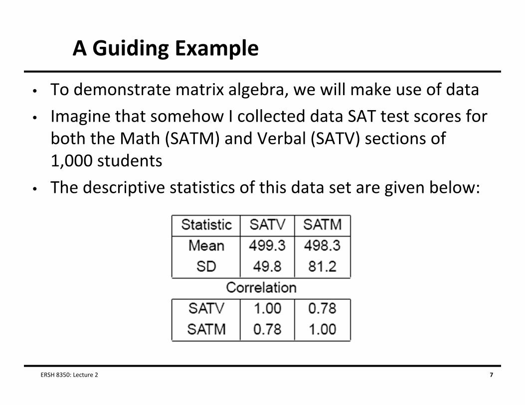
A Guiding Example

• To demonstrate matrix algebra, we will make use of data• Imagine that somehow I collected data SAT test scores for both the Math (SATM) and Verbal (SATV) sections of 1,000 students

• The descriptive statistics of this data set are given below:


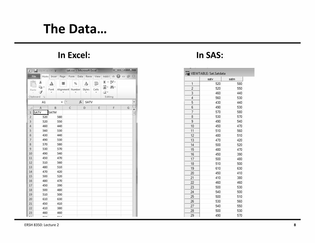
The Data…

In Excel: In SAS:


Matrix Computing: PROC IML

• To help demonstrate the topics we will discuss today, I will beshowing examples in SAS’ proc iml

• The Interactive Matrix Language (IML) is a scientific computing package in SAS that typically used for complicated statistical routines

• Other matrix programs exist ‐ for many statistical applications MATLAB is very useful

• SPSS has matrix computing capabilities, but (in my opinion) it is not as efficient, user friendly, or flexible as SAS proc iml


PROC IML Basics• Proc IML is a proc step in SAS that runs without needing to use

a preliminary data step

• To use IML the following lines of syntax are placed in a SAS file:

• The “reset print;” line makes every result get printed in the output window

• The IML syntax will go between the “reset print;” and the “quit;”


THE BASICS: DEFINITIONS OF MATRICES, VECTORS, AND SCALARS


Matrices• A matrix is a rectangular array of data

Used for storing numbers

• Matrices can have unlimited dimensions For our purposes all matrices will have two dimensions:

Row Columns

• Matrices are symbolized by boldface font in text, typically with capital letters Size (r rows x c columns)

520 580520 550⋮ ⋮

540 660


Vectors

• A vector is a matrix where one dimension is equal to size 1 Column vector: a matrix of size 1

∙

520520⋮

540

Row vector: a matrix of size 1 ∙ 520 580

• Vectors are typically written in boldface font text, usually with lowercase letters


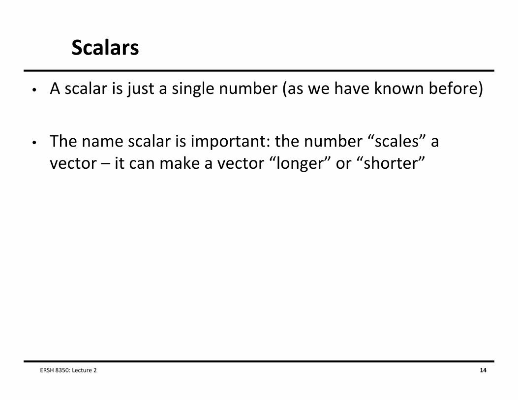
Scalars

• A scalar is just a single number (as we have known before)

• The name scalar is important: the number “scales” a vector – it can make a vector “longer” or “shorter”


Matrix Elements• A matrix (or vector) is composed of a set of elements

Each element is denoted by its position in the matrix (row and column)

• For our matrix of data (size 1000 rows and 2 columns), each element is denoted by:

The first subscript is the index for the rows: i = 1,…,r (= 1000) The second subscript is the index for the columns: j = 1,…,c (= 2)

, ,


Matrix Transpose

• The transpose of a matrix is a reorganization of the matrix by switching the indices for the rows and columns

• An element in the original matrix is now in the transposed matrix


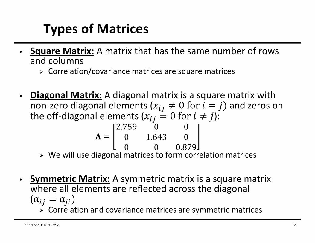
Types of Matrices• Square Matrix: A matrix that has the same number of rows

and columns Correlation/covariance matrices are square matrices

• Diagonal Matrix: A diagonal matrix is a square matrix with non‐zero diagonal elements ( and zeros on the off‐diagonal elements ( ):

2.759 0 00 1.643 00 0 0.879

We will use diagonal matrices to form correlation matrices

• Symmetric Matrix: A symmetric matrix is a square matrix where all elements are reflected across the diagonal ( Correlation and covariance matrices are symmetric matrices


VECTORS


Vectors in Space…

• Vectors (row or column) can be represented as lines on a Cartesian coordinate system

• Consider the vectors: and

• A graph of these vectors would be:

• Question: how would a column vector for each of our example variables (SATM and SATV) be plotted?


Vector Length

• The length of a vector emanating from the origin is given by the Pythagorean formula This is also called the Euclidean distance between the endpoint of the vector and the origin

• From the last slide: ; • From our data:

• In data: length is an analog to the standard deviation In mean‐centered variables, the length is the square root of the sum of mean deviations (not quite the SD, but close)


Vector Addition

• Vectors can be added together so that a new vector is formed

• Vector addition is done element‐wise, by adding each of the respective elements together: The new vector has the same number of rows and columns

12

23

35

Geometrically, this creates a new vector along either of the previous two

• In Data: a new variable (say, SAT total) is the result of vector addition


Vector Multiplication by Scalar

• Vectors can be multiplied by scalars All elements are multiplied by the scalar

2 2 12

24

• Scalar multiplication changes the length of the vector:

• This is where the term scalar comes from: a scalar ends up “rescaling” (resizing) a vector


Linear Combinations

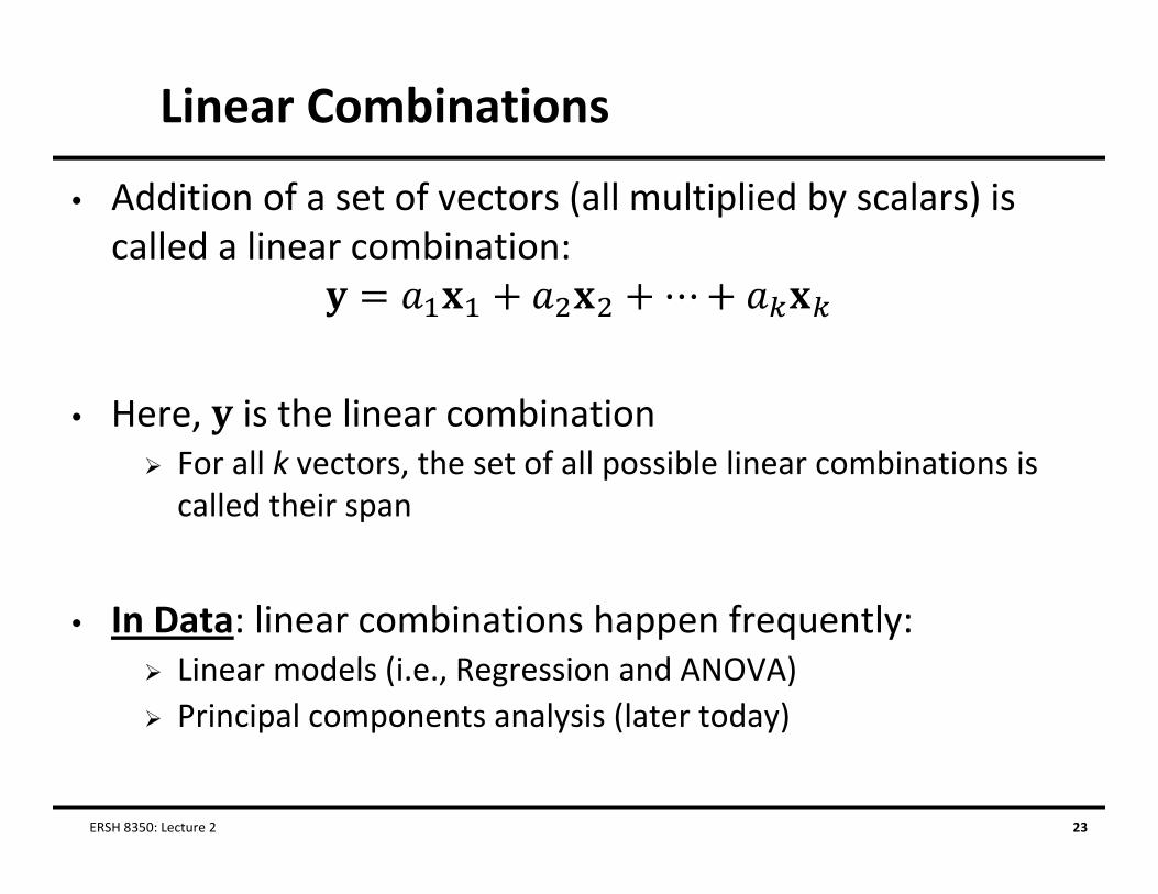
• Addition of a set of vectors (all multiplied by scalars) is called a linear combination:

• Here, is the linear combination For all k vectors, the set of all possible linear combinations is called their span

• In Data: linear combinations happen frequently: Linear models (i.e., Regression and ANOVA) Principal components analysis (later today)


Linear Dependencies

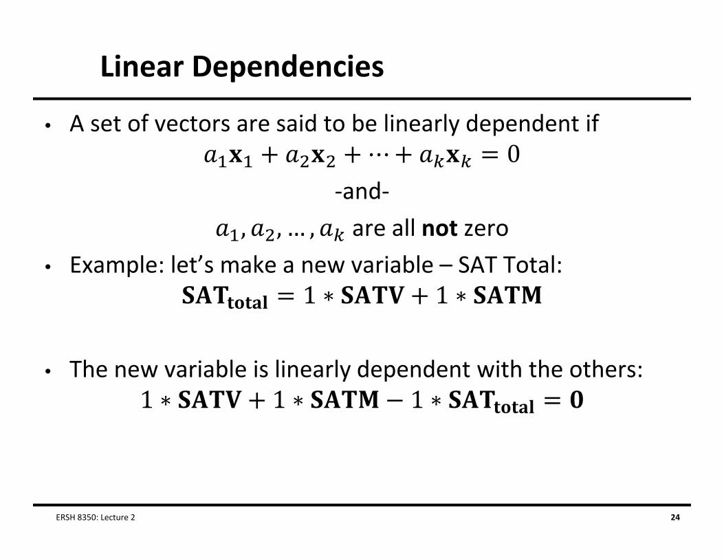
• A set of vectors are said to be linearly dependent if

‐and‐are all not zero

• Example: let’s make a new variable – SAT Total:

• The new variable is linearly dependent with the others:


Normalizing Vectors• Normalizing vectors is the process of rescaling a vector

(multiplication by scalar) so that the length of the vector is equal to one:

• From our example vector:

• As such, the length of the vector is:


Normalizing in Statistics

• We will encounter normalized vectors later today – in principal components analysis

• Generally speaking, entities that have no real space (such as principal components and “latent” factors) have corresponding vectors that are normalized Normalization allows for a solution to be found It’s an arbitrary standard (but one that is well agreed upon)


Inner (Dot) Product of Vectors

• An important concept in vector geometry is that of the inner product of two vectors The inner product is also called the dot product

• The inner product is related to the angle between vectors and to the projection of one vector onto another In data: the angle between vectors is related to the correlation between variables and the projection is related to regression/ANOVA/linear models

• From our example:


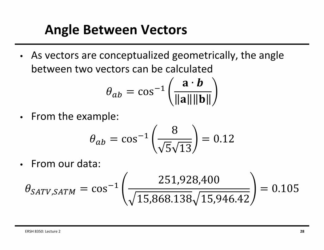
Angle Between Vectors

• As vectors are conceptualized geometrically, the angle between two vectors can be calculated

• From the example:

• From our data:

,


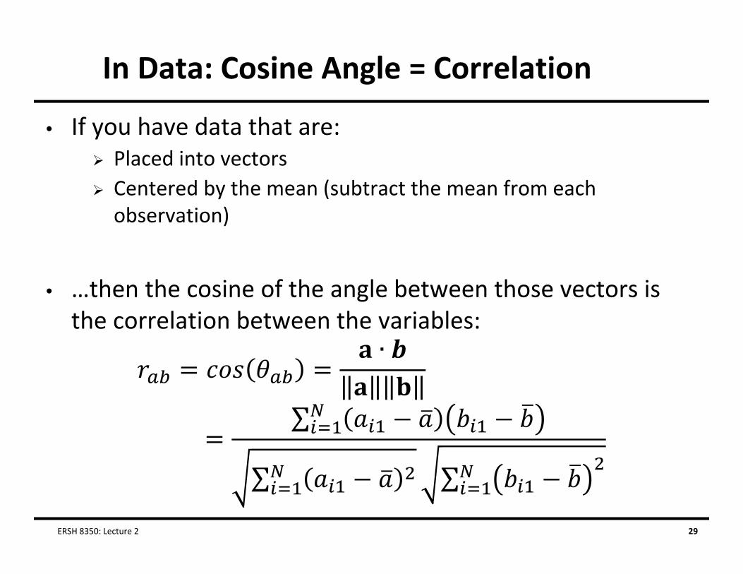
In Data: Cosine Angle = Correlation

• If you have data that are: Placed into vectors Centered by the mean (subtract the mean from each observation)

• …then the cosine of the angle between those vectors is the correlation between the variables:


Vector Projections

• A final vector property that shows up in statistical terms frequently is that of a projection

• The projection of a vector onto is the orthogonal projection of onto the straight line defined by The projection is the “shadow” of one vector onto the other:

• In data: linear models can bethought of as projections


MATRIX ALGEBRA


Moving from Vectors to Matrices• A matrix can be thought of as a collection of vectors

Matrix operations are vector operations on steroids

• Matrix algebra defines a set of operations and entities on matrices I will present a version meant to mirror your previous algebra experiences

• Definitions: Identity matrix Zero vector Ones vector

• Basic Operations: Addition Subtraction Multiplication “Division”


Matrix Addition and Subtraction

• Matrix addition and subtraction are much like vector addition/subtraction

• Rules: Matrices must be the same size (rows and columns)

• Method: The new matrix is constructed of element‐by‐element addition/subtraction of the previous matrices

• Order: The order of the matrices (pre‐ and post‐) does not matter


Matrix Addition/Subtraction


Matrix Multiplication• Matrix multiplication is a bit more complicated

The new matrix may be a different size from either of the two multiplying matrices

• Rules:

Pre‐multiplying matrix must have number of columns equal to the number of rows of the post‐multiplying matrix

• Method: The elements of the new matrix consist of the inner (dot) product of

the row vectors of the pre‐multiplying matrix and the column vectors of the post‐multiplying matrix

• Order: The order of the matrices (pre‐ and post‐) matters


Matrix Multiplication


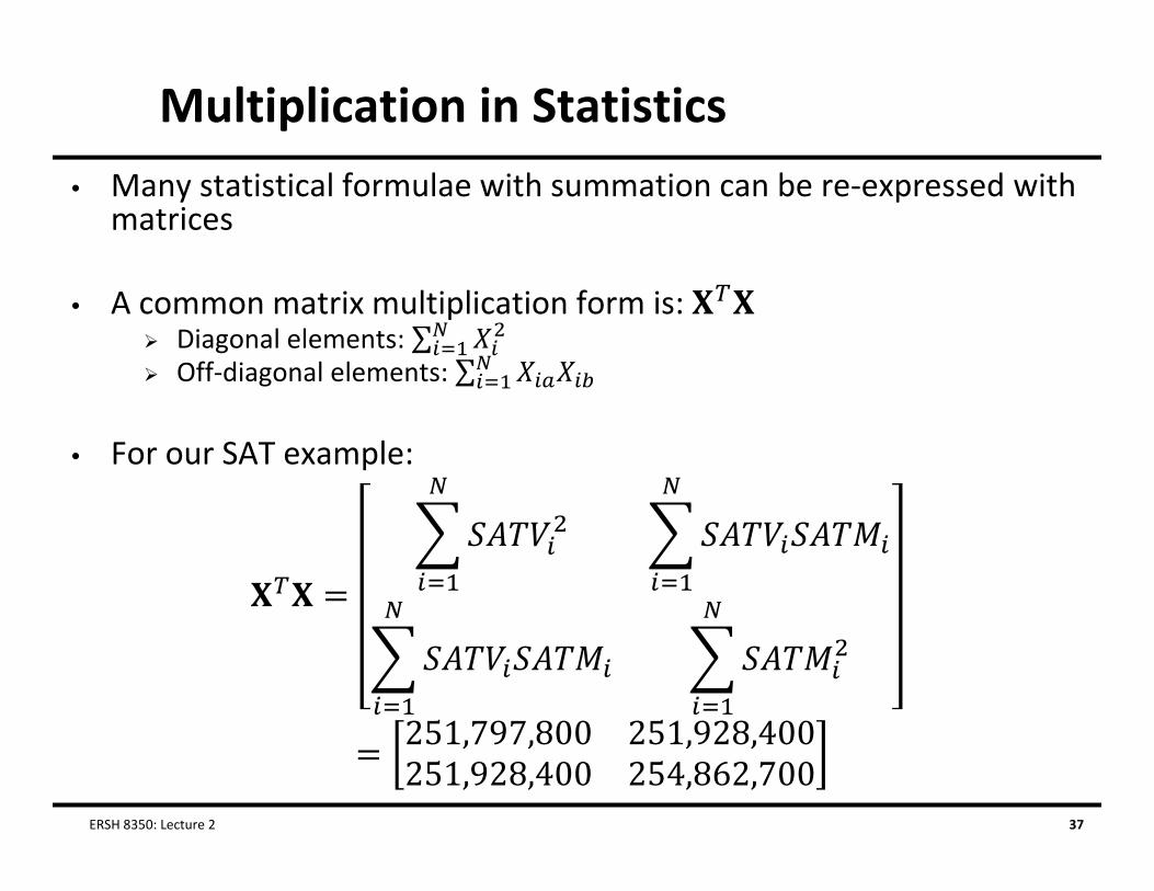
Multiplication in Statistics• Many statistical formulae with summation can be re‐expressed with

matrices

• A common matrix multiplication form is: Diagonal elements: ∑ Off‐diagonal elements: ∑

• For our SAT example:

251,797,800 251,928,400251,928,400 254,862,700


Identity Matrix

• The identity matrix is a matrix that, when pre‐ or post‐multiplied by another matrix results in the original matrix:

• The identity matrix is a square matrix that has: Diagonal elements = 1 Off‐diagonal elements = 0


Zero Vector

• The zero vector is a column vector of zeros

000

• When pre‐ or post‐multiplied the result is the zero vector:


Ones Vector

• A ones vector is a column vector of 1s:

111

• The ones vector is useful for calculating statistical terms, such as the mean vector and the covariance matrix Next class we will discuss what these matrices are, how we compute them, and what the mean


Matrix “Division”: The Inverse Matrix• Division from algebra:

First: Second: 1

• “Division” in matrices serves a similar role For square and symmetric matrices, an inverse matrix is a matrix that when

pre‐ or post‐multiplied with another matrix produces the identity matrix:

• Calculation of the matrix inverse is complicated Even computers have a tough time

• Not all matrices can be inverted Non‐invertable matrices are called singular matrices

In statistics, singular matrices are commonly caused by linear dependencies


The Inverse

• In data: the inverse shows up constantly in statistics Models which assume some type of (multivariate) normality need an inverse covariance matrix

• Using our SAT example Our data matrix was size (1000 x 2), which is not invertable However was size (2 x 2) – square, and symmetric

251,797,800 251,928,400251,928,400 254,862,700

The inverse is:3.61 7 3.57 73.57 7 3.56 7


Matrix Algebra Operations

•

•

•

•

•

•

•

•

•

•

•

• For such that exists:


ADVANCED MATRIX OPERATIONS


Advanced Matrix Functions/Operations

• We end our matrix discussion with some advanced topics All related to multivariate statistical analysis

• To help us throughout, let’s consider the correlation matrix of our SAT data:


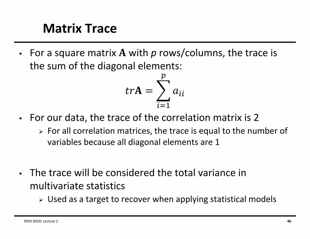
Matrix Trace

• For a square matrix with p rows/columns, the trace is the sum of the diagonal elements:

• For our data, the trace of the correlation matrix is 2 For all correlation matrices, the trace is equal to the number of variables because all diagonal elements are 1

• The trace will be considered the total variance in multivariate statistics Used as a target to recover when applying statistical models


Matrix Determinants• A square matrix can be characterized by a scalar value called a

determinant:det

• Calculation of the determinant is tedious Our determinant was 0.3916

• The determinant is useful in statistics: Shows up in multivariate statistical distributions Is a measure of “generalized” variance of multiple variables

• If the determinant is positive, the matrix is called positive definite Is invertable

• If the determinant is not positive, the matrix is called non‐positive definite Not invertable


Matrix Orthogonality

• A square matrix is said to be orthogonal if:

• Orthogonal matrices are characterized by two properties:1. The dot product of all row vector multiples is the zero vector

Meaning vectors are orthogonal (or uncorrelated)2. For each row vector, the sum of all elements is one

Meaning vectors are “normalized”

• The matrix above is also called orthonormal

• Orthonormal matrices are used in principal components


Eigenvalues and Eigenvectors

• A square matrix can be decomposed into a set of eigenvalues and a set of eigenvectors

• Each eigenvalue has a corresponding eigenvector The number equal to the number of rows/columns of The eigenvectors are all orthogonal

• In many classical multivariate statistics, eigenvalues and eigenvectors are used very frequently We will see their use in principal components shortly


Eigenvalues and Eigenvectors Example

• In our SAT example, the two eigenvalues obtained were:

• The two eigenvectors obtained were:

• These terms will have much greater meaning in one moment (principal components analysis)


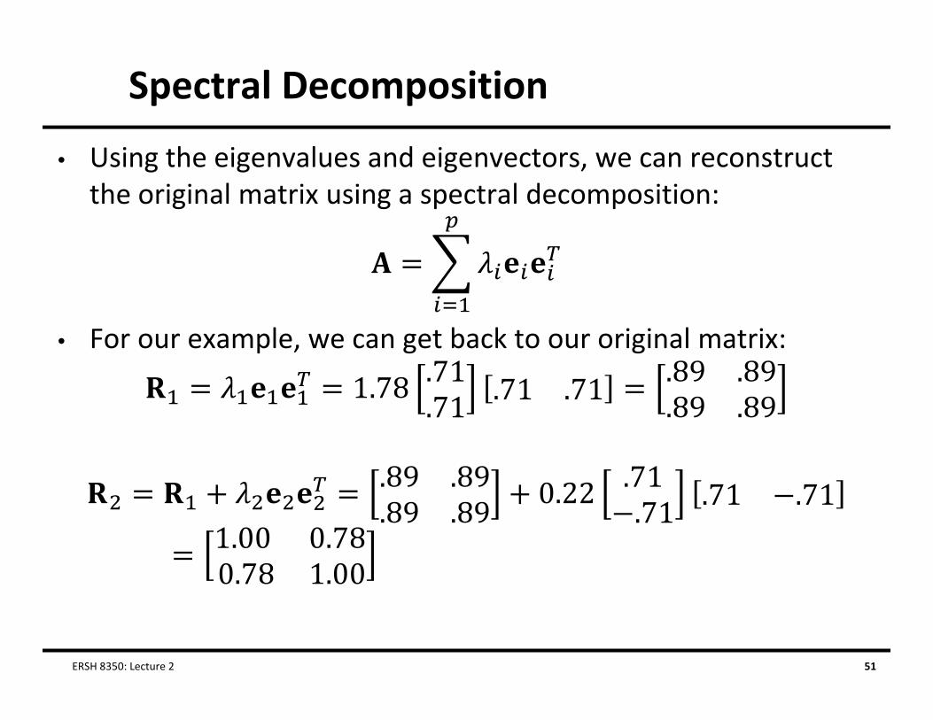
Spectral Decomposition

• Using the eigenvalues and eigenvectors, we can reconstruct the original matrix using a spectral decomposition:

• For our example, we can get back to our original matrix:


Additional Eigenvalue Properties

• The matrix trace can be found by the sum of the eigenvalues:

In our example, the 1.78 .22 2

• The matrix determinant can be found by the product of the eigenvalues

In our example 1.78 ∗ .22 .3916


AN INTRODUCTION TO PRINCIPAL COMPONENTS ANALYSIS


PCA Overview• Principal Components Analysis (PCA) is a method for re‐

expressing the covariance (correlation) between a set of variables The re‐expression comes from creating a set of new variables (linear

combinations) of the original variables

• PCA has two objectives:1. Data reduction

Moving from many original variables down to a few “components”

2. Interpretation Determining which original variables contribute most to thenew “components”

• My objective: use PCA to demonstrate eigenvalues and eigenvectors


Goals of PCA

• The goal of PCA is to find a set of k principal components (composite variables) that: Is much smaller in number than the original set of p variables Accounts for nearly all of the total variance

Total variance = trace of covariance/correlation matrix

• If these two goals can be accomplished, then the set of kprincipal components contains almost as much information as the original p variables Meaning – the components can now replace the original variables in any subsequent analyses


PCA Features

• PCA often reveals relationships between variables that were not previously suspected New interpretations of data and variables often stem from PCA

• PCA usually serves as more of a means to an end rather than an end it itself Components (the new variables) are often used in other statistical techniques Multiple regression Cluster analysis

• Unfortunately, PCA is often intermixed with Exploratory Factor Analysis Don’t. Please don’t. Please help make it stop.


PCA Details

• Notation: let denote our new components and let be our original data matrix (with N observations and p variables) We will let i be our index for a subject

• The new components are linear combinations:

• The weights of the components come from the eigenvectors of the covariance or correlation matrix


Details About the Components• The components are formed by the weights of the

eigenvectors of the covariance or correlation matrix of the original data The variance of a component is given by the eigenvalue associated

with the eigenvector for the component

• Using the eigenvalue and eigenvectors means: Each successive component has lower variance

Var(Y1) > Var(Y2) > … > Var(Yp) All components are uncorrelated The sum of the variances of the principal components is equal to the

total variance:


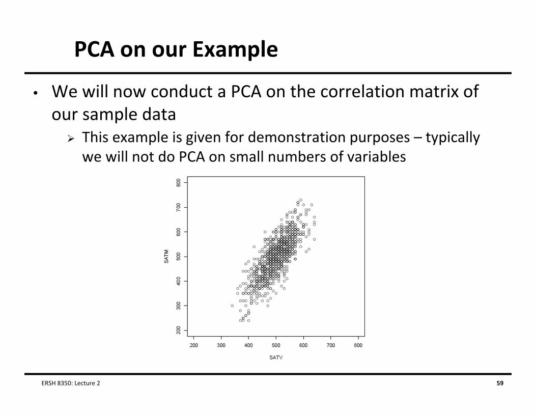
PCA on our Example

• We will now conduct a PCA on the correlation matrix of our sample data This example is given for demonstration purposes – typically we will not do PCA on small numbers of variables


PCA in SAS

• The SAS procedure that does principal components is called proc princomp:

• The results (look familiar?):


Graphical Representation

• Plotting the components and the original data side by side reveals the nature of PCA: Shown from PCA of covariance matrix


PCA Summary

• This introduction to PCA was meant to help describe the nature of eigenvalues and eigenvectors Many classical multivariate statistics use these terms

• We will return to PCA in the 3rd part of class – when we discuss inferences about covariances in multivariate data

• Eigenvalues and eigenvectors will reappear in the next 2‐3 weeks The basis for classical Multivariate ANOVA Modern versions have moved away from these terms

But they still are useful


Wrapping Up• Matrix algebra is the language of multivariate statistics

Learning the basics will help you read work (both new old)

• Over the course of the semester, we will use matrixalgebra frequently It provides for more concise formulae

• In practice, we will use matrix algebra very little But understanding how it works is the key to understanding how

statistical methods work and are related

• Up next: statistical terms and statistical distributions (univariate and multivariate) The basis for modern estimation methods using maximum likelihood

or Bayesian estimation


A Introduction to Matrix Algebra Principal Components … · A Introduction to Matrix Algebra and...

Documents

Transcript of A Introduction to Matrix Algebra Principal Components … · A Introduction to Matrix Algebra and...