A INTRODUCTION TO BUSINESS MATHEMATICS … · Introduction These lecture notes contain the entire...

arX

iv:1

509.

0433

3v2

[q-f

in.G

N]

16 S

ep 2

015

AN INTRODUCTION TO

BUSINESSMATHEMATICS

Lecture notes for the Bachelor degree programmesIB/IMC/IMA/ITM/IEVM/ACM/IEM/IMMat Karlshochschule International University

Module

0.1.1 IMQM: Introduction to Management and its Quantitative Methods

HENK VAN ELST

August 30, 2015

Fakultat I: Betriebswirtschaft und ManagementKarlshochschule

International UniversityKarlstraße 36–3876133 Karlsruhe

Germany

E–mail:[email protected]

E–Print: arXiv:1509.04333v2 [q-fin.GN]

c© 2009–2015 Karlshochschule International University and Henk van Elst

http://arxiv.org/abs/1509.04333v2

http://arxiv.org/abs/1509.04333

Abstract

These lecture notes provide a self-contained introductionto the mathematical methods required in a Bachelordegree programme in Business, Economics, or Management. Inparticular, the topics covered comprise real-valued vector and matrix algebra, systems of linear algebraic equations, Leontief’s stationary input–outputmatrix model, linear programming, elementary financial mathematics, as well as differential and integralcalculus of real-valued functions of one real variable. A special focus is set on applications in quantitativeeconomical modelling.

Cite as:arXiv:1509.04333v2 [q-fin.GN]

These lecture notes were typeset in LATEX 2ε.


Contents

Abstract

Qualification objectives of the module (excerpt) 1

Introduction 2

1 Vector algebra in Euclidian spaceRn 51.1 Basic concepts . . . . . . . . . . . . . . . . . . . . . . . . . . . . . . . . . . .. 51.2 Dimension and basis ofRn . . . . . . . . . . . . . . . . . . . . . . . . . . . . . . 71.3 Euclidian scalar product . . . . . . . . . . . . . . . . . . . . . . . . . .. . . . . 8

2 Matrices 112.1 Matrices as linear mappings . . . . . . . . . . . . . . . . . . . . . . . .. . . . . 112.2 Basic concepts . . . . . . . . . . . . . . . . . . . . . . . . . . . . . . . . . . .. 132.3 Matrix multiplication . . . . . . . . . . . . . . . . . . . . . . . . . . . .. . . . . 14

3 Systems of linear algebraic equations 173.1 Basic concepts . . . . . . . . . . . . . . . . . . . . . . . . . . . . . . . . . . .. 173.2 Gaußian elimination . . . . . . . . . . . . . . . . . . . . . . . . . . . . . .. . . . 183.3 Rank of a matrix . . . . . . . . . . . . . . . . . . . . . . . . . . . . . . . . . . .193.4 Solution criteria . . . . . . . . . . . . . . . . . . . . . . . . . . . . . . . .. . . . 203.5 Inverse of a regular(n× n)-matrix . . . . . . . . . . . . . . . . . . . . . . . . . . 213.6 Outlook . . . . . . . . . . . . . . . . . . . . . . . . . . . . . . . . . . . . . . . . 22

4 Leontief’s input–output matrix model 254.1 General considerations . . . . . . . . . . . . . . . . . . . . . . . . . . .. . . . . 254.2 Input–output matrix and resource consumption matrix . .. . . . . . . . . . . . . . 26

4.2.1 Input–output matrix . . . . . . . . . . . . . . . . . . . . . . . . . . . .. 264.2.2 Resource consumption matrix . . . . . . . . . . . . . . . . . . . . .. . . 28

4.3 Stationary linear flows of goods . . . . . . . . . . . . . . . . . . . . .. . . . . . 294.3.1 Flows of goods: endogenous INPUT to total OUTPUT . . . . .. . . . . . 294.3.2 Flows of goods: exogenous INPUT to total OUTPUT . . . . . .. . . . . . 30

4.4 Outlook . . . . . . . . . . . . . . . . . . . . . . . . . . . . . . . . . . . . . . . . 30

CONTENTS

5 Linear programming 335.1 Exposition of a quantitative problem . . . . . . . . . . . . . . . .. . . . . . . . . 335.2 Graphical solution method . . . . . . . . . . . . . . . . . . . . . . . . .. . . . . 355.3 Dantzig’s simplex algorithm . . . . . . . . . . . . . . . . . . . . . . .. . . . . . 36

6 Elementary financial mathematics 396.1 Arithmetical and geometrical sequences and series . . . .. . . . . . . . . . . . . 39

6.1.1 Arithmetical sequence and series . . . . . . . . . . . . . . . . .. . . . . . 396.1.2 Geometrical sequence and series . . . . . . . . . . . . . . . . . .. . . . . 40

6.2 Interest and compound interest . . . . . . . . . . . . . . . . . . . . .. . . . . . . 416.3 Redemption payments in constant annuities . . . . . . . . . . .. . . . . . . . . . 436.4 Pension calculations . . . . . . . . . . . . . . . . . . . . . . . . . . . . .. . . . . 466.5 Linear and declining-balance depreciation methods . . .. . . . . . . . . . . . . . 48

6.5.1 Linear depreciation method . . . . . . . . . . . . . . . . . . . . . .. . . 486.5.2 Declining-balance depreciation method . . . . . . . . . . .. . . . . . . . 48

6.6 Summarising formula . . . . . . . . . . . . . . . . . . . . . . . . . . . . . .. . . 49

7 Differential calculus of real-valued functions 517.1 Real-valued functions . . . . . . . . . . . . . . . . . . . . . . . . . . . .. . . . . 51

7.1.1 Polynomials of degreen . . . . . . . . . . . . . . . . . . . . . . . . . . . 527.1.2 Rational functions . . . . . . . . . . . . . . . . . . . . . . . . . . . . .. 537.1.3 Power-law functions . . . . . . . . . . . . . . . . . . . . . . . . . . . .. 537.1.4 Exponential functions . . . . . . . . . . . . . . . . . . . . . . . . . .. . 537.1.5 Logarithmic functions . . . . . . . . . . . . . . . . . . . . . . . . . .. . 547.1.6 Concatenations of real-valued functions . . . . . . . . . .. . . . . . . . . 54

7.2 Derivation of differentiable real-valued functions . .. . . . . . . . . . . . . . . . 557.3 Common functions in economic theory . . . . . . . . . . . . . . . . .. . . . . . . 577.4 Curve sketching . . . . . . . . . . . . . . . . . . . . . . . . . . . . . . . . . .. . 587.5 Analytic investigations of economic functions . . . . . . .. . . . . . . . . . . . . 59

7.5.1 Total cost functions according to Turgot and von Thunen . . . . . . . . . . 597.5.2 Profit functions in the diminishing returns picture . .. . . . . . . . . . . . 627.5.3 Extremal values of rational economic functions . . . . .. . . . . . . . . . 64

7.6 Elasticities . . . . . . . . . . . . . . . . . . . . . . . . . . . . . . . . . . . .. . . 65

8 Integral calculus of real-valued functions 718.1 Indefinite integrals . . . . . . . . . . . . . . . . . . . . . . . . . . . . . .. . . . 718.2 Definite integrals . . . . . . . . . . . . . . . . . . . . . . . . . . . . . . . .. . . 728.3 Applications in economic theory . . . . . . . . . . . . . . . . . . . .. . . . . . . 73

A Glossary of technical terms (GB – D) 75

Bibliography 81

Qualification objectives of the module(excerpt)

The qualification objectives shall be reached by an integrative approach.

A broad instructive range is aspired. The students shall acquire a 360 degree orientation concerningthe task- and personnel-related tasks and roles of a managerand supporting tools and methods andbe able to describe the coherence in an integrative way. The knowledge concerning the tasks andthe understanding of methods and tools shall be strengthened by a constructivist approach basedon case studies and exercises.

Students who have successfully participated in this modulewill be able to

• . . . ,

• solve problems in Linear Algebra and Analysis and apply suchmathematical methods toquantitative problems in management.

• apply and challenge the knowledge critically on current issues and selected case studies.

1

2 CONTENTS

Introduction

These lecture notes contain the entire material of the quantitative methods part of the first semestermodule0.1.1 IMQM: Introduction to Management and its Quantitativ e Methods at Karl-shochschule International University. The aim is to provide a selection of tried-and-tested math-ematical tools that proved efficient in actual practical problems ofEconomicsandManagement.These tools constitute the foundation for a systematic treatment of the typical kinds of quantita-tive problems one is confronted with in a Bachelor degree programme. Nevertheless, they providea sufficient amount of points of contact with a quantitatively oriented subsequent Master degreeprogramme inEconomics, Management, or theSocial Sciences.

The prerequisites for a proper understanding of these lecture notes are modest, as they do not gomuch beyond the basic A-levels standards inMathematics. Besides the four fundamental arith-metical operations of addition, subtraction, multiplication and division of real numbers, you shouldbe familiar, e.g., with manipulating fractions, dealing with powers of real numbers, the binomialformulae, determining the point of intersection for two straight lines in the Euclidian plane, solv-ing a quadratic algebraic equation, and the rules of differentiation of real-valued functions of onevariable.

It might be useful for the reader to have available a moderngraphic display calculator (GDC) fordealing with some of the calculations that necessarily arise along the way, when confronted withspecific quantitative problems. Some current models used inpublic schools and in undergraduatestudies are, amongst others,

• Texas InstrumentsTI–84 plus,

• CasioCFX–9850GB PLUS.

However, the reader is strongly encouraged to think about resorting, as an alternative, to aspread-sheet programmesuch as EXCEL or OpenOffice to handle the calculations one encounters inone’s quantitative work.

The central theme of these lecture notes is the acquisition and application of a number of effec-tive mathematical methods in a business oriented environment. In particular, we hereby focus onquantitative processesof the sort

INPUT → OUTPUT ,

for which different kinds offunctional relationships between some numericalINPUT quantitiesand some numericalOUTPUT quantities are being considered. Of special interest in this context

3

4 CONTENTS

will be ratios of the structureOUTPUTINPUT

.

In this respect, it is a general objective inEconomicsto look for ways to optimise the value ofsuch ratios (in favour of someeconomic agent), either by seeking to increase the OUTPUT whenthe INPUT is confined to be fixed, or by seeking to decrease the INPUT when the OUTPUT isconfined to be fixed. Consequently, most of the subsequent considerations in these lecture noteswill therefore deal with issues ofoptimisation of given functional relationships between somevariables, which manifest themselves either inminimisation or in maximisation procedures.

The structure of these lecture notes is the following. Part Ipresents selected mathematical methodsfrom Linear Algebra , which are discussed in Chs. 1 to 5. Applications of these methods focus onthe quantitative aspects of flows of goods in simple economicmodels, as well as on problems inlinear programming. In Part II, which is limited to Ch. 6, we turn to discuss elementary aspectsof Financial Mathematics. Fundamental principles ofAnalysis, comprising differential and in-tegral calculus for real-valued functions of one real variable, and their application to quantitativeeconomic problems, are reviewed in Part III; this extends across Chs. 7 and 8.

We emphasise the fact that there areno explicit examples nor exercises included in these lecturenotes. These are reserved exclusively for the lectures given throughout term time.

Recommended textbooks accompanying the lectures are the works by Asano (2013) [2], Dowl-ing (2009) [11], Dowling (1990) [10], Baueret al (2008) [3], Bosch (2003) [6], and Hulsmannet al (2005) [16]. Some standard references ofApplied Mathematics are, e.g., Bronsteinet al(2005) [7] and Arenset al (2008) [1]. Should the reader feel inspired by the aesthetics, beauty,ellegance and efficiency of the mathematical methods presented, and, hence, would like to knowmore about their background and relevance, as well as being introduced to further mathematicaltechniques of interest, she/he is recommended to take a lookat the brilliant books by Penrose(2004) [21], Singh (1997) [23], Gleick(1987) [13] and Smith(2007) [24]. Note that most of thetextbooks and monographs mentioned in this Introduction are available from the library at Karl-shochschule International University.

Finally, we draw the reader’s attention to the fact that the *.pdf version of these lecture notes con-tains interactive features such as fully hyperlinked references to original publications at the web-sitesdx.doi.org andjstor.org, as well as active links to biographical information on sci-entists that have been influential in the historical development ofMathematics, hosted by the web-sites The MacTutor History of Mathematics archive (www-history.mcs.st-and.ac.uk)anden.wikipedia.org.

http://dx.doi.org

http://www.jstor.org

http://www-history.mcs.st-and.ac.uk/

http://en.wikipedia.org/wiki/Main_Page

Chapter 1

Vector algebra in Euclidian spaceRn

Let us begin our elementary considerations ofvector algebra with the introduction of a specialclass of mathematical objects. These will be useful at a later stage, when we turn to formulatecertain problems of a quantitative nature in a compact and elegant way. Besides introducing thesemathematical objects, we also need to define which kinds of mathematical operations they can besubjected to, and what computational rules we have to take care of.

1.1 Basic concepts

Given be a setV of mathematical objectsa which, for now, we want to consider merely as acollection ofn arbitrary real numbersa1, . . . ,ai, . . . ,an. In explicit terms,

V =

a =

a1...ai...an

| ai ∈ R, i = 1, . . . , n

. (1.1)

Formally then real numbers considered can either be assembled in an ordered pattern as a columnor a row. We define

Def.: Real-valuedcolumn vectorwith n components

a :=

a1...ai...an

, ai ∈ R, i = 1, . . . , n , (1.2)

Notation:a ∈ Rn×1,

and

5

6 CHAPTER 1. VECTOR ALGEBRA IN EUCLIDIAN SPACERN

Def.: Real-valuedrow vector with n components

aT := (a1, . . . , ai, . . . , an) , ai ∈ R, i = 1, . . . , n , (1.3)

Notation:aT ∈ R1×n.

Correspondingly, we define then-component objects

0 :=

0...0...0

and 0T := (0, . . . , 0, . . . , 0) (1.4)

to constitute relatedzero vectors.

Next we define for like objects in the setV , i.e., either forn-component column vectors or forn-component row vectors, two simple computational operations. These are

Def.: Addition of vectors

a+ b :=

a1...ai...an

+

b1...bi...bn

=

a1 + b1...

ai + bi...

an + bn

, ai, bi ∈ R , (1.5)

and

Def.: Rescalingof vectors

λa :=

λa1...

λai...

λan

, λ, ai ∈ R . (1.6)

The rescaling of a vectora with an arbitrary non-zero real numberλ has the following effects:

• |λ| > 1 — stretching of the length ofa

• 0 < |λ| < 1 — shrinking of the length ofa

• λ < 0 — directional reversal ofa.

1.2. DIMENSION AND BASIS OFRN 7

The notion of the length of a vectora will be made precise shortly.

The addition and the rescaling ofn-component vectors satisfy the following addition and multipli-cation laws:

Computational rules for addition and rescaling of vectorsFor vectorsa, b, c ∈ R

n:

1. a+ b = b+ a (commutative addition)

2. a+ (b+ c) = (a+ b) + c (associative addition)

3. a+ 0 = a (addition identity element)

4. For everya, b ∈ Rn, there exists exactly onex ∈ R

n such thata + x = b

(invertibility of addition )

5. (λµ)a = λ(µa) with λ ∈ R (associative rescaling)

6. 1a = a (rescaling identity element)

7. λ(a+ b) = λa+ λb;

(λ+ µ)a = λa+ µa with λ, µ ∈ R (distributive rescaling).

In conclusion of this section, we remark that every set of mathematical objectsV constructed inline with Eq. (1.1), with an addition and a rescaling defined according to Eqs. (1.5) and (1.6), andsatisfying the laws stated above, constitutes alinear vector space over Euclidian spaceRn.1

1.2 Dimension and basis ofRn

Let there be givenm n-component vectors2 a1, . . . ,ai, . . . ,am ∈ Rn, as well asm real numbers

λ1, . . . , λi, . . . , λm ∈ R. The newn-component vectorb resulting from the addition of arbitrarilyrescaled versions of thesem vectors according to

b = λ1a1 + . . .+ λiai + . . .+ λmam =:

m∑

i=1

λiai ∈ Rn (1.7)

is referred to as alinear combination of them vectorsai, i = 1, . . . , m.

Def.: A set ofm vectorsa1, . . . ,ai, . . . ,am ∈ Rn is calledlinearly independent when the condi-

tion

0!= λ1a1 + . . .+ λiai + . . .+ λmam =

m∑

i=1

λiai , (1.8)

1This is named after the ancient greek mathematician Euclid of Alexandria (about 325 BC–265 BC).2A slightly s horter notation forn-component column vectorsa ∈ R

n×1 is given bya ∈ Rn; likewiseaT ∈ R

n

for n-component row vectorsaT ∈ R1×n.

http://www-groups.dcs.st-and.ac.uk/~history/Biographies/Euclid.html


i.e., the problem of forming thezero vector0 ∈ Rn from a linear combination of them vectors

a1, . . . ,ai, . . . ,am ∈ Rn, canonlybe solved trivially, namely by0 = λ1 = . . . = λi = . . . = λm.

When, however, this condition can be solved non-trivially,with someλi 6= 0, then the set ofmvectorsa1, . . . ,ai, . . . ,am ∈ R

n is calledlinearly dependent.

In Euclidian spaceRn, there is a maximum numbern (!) of vectors which can be linearly indepen-dent. This maximum number is referred to as thedimension of Euclidian spaceRn. Every setof n linearly independent vectors in Euclidian spaceR

n constitutes a possiblebasis of EuclidianspaceRn. If the set{a1, . . . ,ai, . . . ,an} constitutes a basis ofRn, then every other vectorb ∈ R

n

can be expressed in terms of these basis vectors by

b = β1a1 + . . .+ βiai + . . .+ βnan =

n∑

i=1

βiai . (1.9)

The rescaling factorsβi ∈ R of theai ∈ Rn are called thecomponents of vectorb with respect

to the basis{a1, . . . ,ai, . . . ,an}.

Remark: Then unit vectors

e1 :=

10...0

, e2 :=

01...0

, . . . , en :=

00...1

, (1.10)

constitute the so-calledcanonical basis of Euclidian spaceRn. With respect to this basis, allvectorsb ∈ R

n can be represented as a linear combinationen

b =

b1b2...bn

= b1e1 + b2e2 + · · ·+ bnen =n∑

i=1

biei . (1.11)

1.3 Euclidian scalar product

Finally, to conclude this section, we introduce a third mathematical operation defined for vectorsonR

n.

Def.: For ann-component row vectoraT ∈ R1×n and ann-component column vectorb ∈ R

n×1,theEuclidian scalar product

aT · b := (a1, . . . , ai, . . . an)

b1...bi...bn

= a1b1 + . . .+ aibi . . .+ anbn =:n∑

i=1

aibi (1.12)

1.3. EUCLIDIAN SCALAR PRODUCT 9

defines a mappingf : R1×n × Rn×1 → R from the product set ofn-component row and column

vectors to the set of real numbers. Note that, in contrast to the addition and the rescaling ofn-component vectors, the outcome of forming a Euclidian scalar product between twon-componentvectors is asingle real number.

In the context of the Euclidian scalar product, two non-zerovectorsa, b ∈ Rn (wit a 6= 0 6= b)

are referred to asmutually orthogonal when they exhibit the property that0 = aT · b = bT · a.

Computational rules for Euclidian scalar product of vectorsFor vectorsa, b, c ∈ R

n:

1. (a+ b)T · c = aT · c + bT · c (distributive scalar product )

2. aT · b = bT · a (commutative scalar product)

3. (λaT ) · b = λ(aT · b) with λ ∈ R (homogeneous scalar product)

4. aT · a > 0 for all a 6= 0 (positive definite scalar product).

Now we turn to introduce the notion of the length of ann-component vector.

Def.: The length of a vectora ∈ Rn is defined via the Euclidian scalar product as

|a| :=√aT · a =

√

a21 + . . .+ a2i + . . .+ a2n =:

√√√√

n∑

i=1

a2i . (1.13)

Technically one refers to the non-negative real number|a| as theabsolute valueor theEuclidiannorm of the vectora ∈ R

n. The length ofa ∈ Rn has the following properties:

• |a| ≥ 0, and|a| = 0 ⇔ a = 0;

• |λa| = |λ||a| for λ ∈ R;

• |a+ b| ≤ |a|+ |b| (triangle inequality ).

Every non-zero vectora ∈ Rn, i.e., |a| > 0, can be rescaled by the reciprocal of its length. This

procedure defines the

Def.: Normalisation of a vectora ∈ Rn;

a :=a

|a| ⇒ |a| = 1 . (1.14)

By this method one generates a vector of length1, i.e., aunit vector a. To denote unit vectors wewill employ the “hat” symbol.

Lastly, also by means of the Euclidian scalar product, we introduce the angle enclosed betweentwo non-zero vectors.


Def.: Angle enclosed betweena, b 6= 0 ∈ Rn

cos[ϕ(a, b)] =aT

|a| ·b

|b| = aT · b ⇒ ϕ(a, b) = cos−1(aT · b) . (1.15)

Remark: The inverse cosine function3 cos−1(. . .) is available on every standard GDC or spread-sheet.

3The notion of on inverse function will be discussed later in Ch. 7.

Chapter 2

Matrices

In this chapter, we introduce a second class of mathematicalobjects that are more general thanvectors. For these objects, we will also define certain mathematical operations, and a set of com-putational rules that apply in this context.

2.1 Matrices as linear mappings

Consider given a collection ofm × n arbitrary real numbersa11, a12 . . . , aij , . . . ,amn, which wearrange systematically in a particular kind of array.

Def.: A real-valued(m × n)-matrix is formally defined to constitute an array of real numbersaccording to

A :=

a11 a12 . . . a1j . . . a1na21 a22 . . . a2j . . . a2n...

.... . .

.... . .

...ai1 ai2 . . . aij . . . ain...

.... . .

.... . .

...am1 am2 . . . amj . . . amn

, (2.1)

whereaij ∈ R, i = 1, . . . , m; j = 1, . . . , n.Notation:A ∈ R

m×n.

Characteristic features of this array of real numbers are:

• m denotes the number ofrows of A, n the number ofcolumnsof A.

• aij represents theelementsof A; aij is located at the point of intersection of theith row andthejth column ofA.

• elements of theith row constitute therow vector (ai1, ai2, . . . , aij, . . . , ain), elements of the

11

12 CHAPTER 2. MATRICES

jth column thecolumn vector

a1ja2j...aij...

amj

.

Formally column vectors need to be viewed as(n× 1)-matrices, row vectors as(1× n)-matrices.An (m × n)-zero matrix, denoted by0, has all its elements equal to zero, i.e.,

0 :=

0 0 . . . 00 0 . . . 0...

.... . .

...0 0 . . . 0

. (2.2)

Matrices which have anequal number of rows and columns, i.e.m = n, are referred to asquadratic matrices. In particular, the(n × n)-unit matrix (or identity matrix)

1 :=

1 0 . . . 0 . . . 00 1 . . . 0 . . . 0...

.... . .

.... . .

...0 0 . . . 1 . . . 0...

.... . .

.... . .

...0 0 . . . 0 . . . 1

(2.3)

holds a special status in the family of(n× n)-matrices.

Now we make explicit in what sense we will comprehend(m × n)-matrices as mathematicalobjects.

Def.: A real-valued matrixA ∈ Rm×n defines by the computational operation

Ax :=

a11 a12 . . . a1j . . . a1na21 a22 . . . a2j . . . a2n...

.... . .

.... . .

...ai1 ai2 . . . aij . . . ain...

.... . .

.... . .

...am1 am2 . . . amj . . . amn

x1

x2...xj...xn

:=

a11x1 + a12x2 + . . .+ a1jxj + . . .+ a1nxn

a21x1 + a22x2 + . . .+ a2jxj + . . .+ a2nxn...

ai1x1 + ai2x2 + . . .+ aijxj + . . .+ ainxn...

am1x1 + am2x2 + . . .+ amjxj + . . .+ amnxn

=:

y1y2...yi...ym

= y (2.4)

2.2. BASIC CONCEPTS 13

a mapping A : Rn×1 → Rm×1, i.e. a mapping from the set of real-valuedn-component column

vectors (here:x) to the set of real-valuedm-component column vectors (here:y).

In loose analogy to the photographic process,x can be viewed as representing an “object,”A a“camera,” andy the resultant “image.”

Since for real-valued vectorsx1,x2 ∈ Rn×1 and real numbersλ ∈ R, mappings defined by real-

valued matricesA ∈ Rm×n exhibit the two special properties

A(x1 + x2) = (Ax1) + (Ax2)

A(λx1) = λ(Ax1) ,(2.5)

they constitutelinear mappings.1

We now turn to discuss the most important mathematical operations defined for(m× n)-matrices,as well as the computational rules that obtain.

2.2 Basic concepts

Def.: Transposeof a matrixForA ∈ R

m×n, we define the process of transposingA by

AT : aTij := aji , (2.6)

wherei = 1, . . . , m undj = 1, . . . , n. Note that it holds thatAT ∈ Rn×m.

When transposing an(m×n)-matrix, one simply has to exchange the matrix’ rows with itscolumns(and vice versa): the elements of the first row become the elements of the first column, etc. Itfollows that, in particular,

(AT )T = A (2.7)

applies.

Two special cases may occur for quadratic matrices (wherem = n):

• WhenAT = A, one refers toA as asymmetric matrix .

• WhenAT = −A, one refers toA as anantisymmetric matrix .

Def.: Addition of matricesForA,B ∈ R

m×n, the sum is given by

A+B =: C : aij + bij =: cij , (2.8)

with i = 1, . . . , m andj = 1, . . . , n.

Note that an addition can be performed meaningfully only formatrices of thesame format.

1It is important to note at this point that many advanced mathematical models designed to describe quantitativeaspects of some natural and economic phenomena donot satisfy the conditions (2.5), as they employnon-linearmappingsfor this purpose. However, in such contexts, linear mappings often provide useful first approximations.


Def.: Rescalingof matricesForA ∈ R

m×n andλ ∈ R\{0}, let

λA =: C : λaij =: cij , (2.9)

wherei = 1, . . . , m andj = 1, . . . , n.

When rescaling a matrix, all its elements simply have to be multiplied by the same non-zero realnumberλ.

Computational rules for addition and rescaling of matricesFor matricesA,B,C ∈ R

m×n:

1. A+B = B+A (commutative addition)

2. A+ (B+C) = (A+B) +C (associative addition)

3. A+ 0 = A (addition identity element)

4. For everyA andB, there exists exactly oneZ such thatA+ Z = B.

(invertibility of addition )

5. (λµ)A = λ(µA) with λ, µ ∈ R\{0} (associative rescaling)

6. 1A = A (rescaling identity element)

7. λ(A+B) = λA+ λB;

(λ+ µ)A = λA+ µA with λ, µ ∈ R\{0} (distributive rescaling)

8. (A+B)T = AT +BT (transposition rule 1)

9. (λA)T = λAT with λ ∈ R\{0}. (transposition rule 2)

Next we introduce a particularly useful mathematical operation for matrices.

2.3 Matrix multiplication

Def.: For a real-valued(m× n)-matrixA and a real-valued(n× r)-matrixB, amatrix multipli-cation is defined by

AB =: C

ai1b1j + . . .+ aikbkj + . . .+ ainbnj =:∑n

k=1 aikbkj =: cij ,(2.10)

with i = 1, . . . , m andj = 1, . . . , r, thus yielding as an outcome a real-valued(m× r)-matrixC.

2.3. MATRIX MULTIPLICATION 15

The element ofC at the intersection of theith row and thejth column is determined by thecomputational rule

cij = Euclidian scalar product ofith row vector ofA andjth column vector ofB . (2.11)

It is important to realise that the definition of a matrix multiplication just provided depends inan essential way on the fact thatmatrix A on the left in the product needs to have as many (!)columns as matrixB on the right rows. Otherwise, a matrix multiplicationcannotbe defined in ameaningful way.

GDC: For matrices[A] and[B] edited beforehand, of matching formats, their matrix multiplicationcan be evaluated in modeMATRIX→ NAMES by [A] ∗ [B].

Computational rules for matrix multiplicationForA,B,C real-valued matrices of correspondingly matching formatswe have:

1. AB = 0 is possible withA 6= 0,B 6= 0. (zero divisor)

2. A(BC) = (AB)C (associative matrix multiplication)

3. A 1︸︷︷︸

∈Rn×n

= 1︸︷︷︸

∈Rm×m

A = A (multiplicative identity element)

4. (A+B)C = AC+BC

C(A+B) = CA+CB (distributive matrix multiplication )

5. A(λB) = (λA)B = λ(AB) with λ ∈ R (homogeneous matrix multiplication)

6. (AB)T = BTAT (transposition rule).

Chapter 3

Systems of linear algebraic equations

In this chapter, we turn to address a particular field of application of the notions of matrices andvectors, or of linear mappings in general.

3.1 Basic concepts

Let us begin with a system ofm ∈ N linear algebraic equations, wherein every single equation canbe understood to constitute aconstraint on the range of values ofn ∈ N variablesx1, . . . , xn ∈ R.The objective is to determine all possible values ofx1, . . . , xn ∈ R which satisfy these constraintssimultaneously. Problems of this kind, namelysystems of linear algebraic equations, are oftenrepresented in the form

• Representation 1:

a11x1 + . . .+ a1jxj + . . .+ a1nxn = b1...

ai1x1 + . . .+ aijxj + . . .+ ainxn = bi (3.1)...

am1x1 + . . .+ amjxj + . . .+ amnxn = bm .

Depending on how the natural numbersm andn relate to one another, systems of linear algebraicequations can be classified as follows:

• m < n: fewer equations than variables; the linear system isunder-determined,

• m = n: same number of equations as variables; the linear system iswell-determined,

• m > n: more equations than variables; the linear system isover-determined.

A more compact representation of a linear system of format(m× n) is given by

17

18 CHAPTER 3. SYSTEMS OF LINEAR ALGEBRAIC EQUATIONS

• Representation 2:

Ax =

a11 . . . a1j . . . a1n...

. . ....

. . ....

ai1 . . . aij . . . ain...

. . ....

. . ....

am1 . . . amj . . . amn

x1...xj...xn

=

b1...bi...bm

= b . (3.2)

The mathematical objects employed in this variant of a linear system are as follows:A takes thecentral role of thecoefficient matrix of the linear system, of format(m × n), x is its variablevector, of format(n× 1), and, lastly,b is its image vector, of format(m× 1).

When dealing with systems of linear algebraic equations in the form of Representation 2, i.e.Ax = b, the main question to be answered is:

Question: For givencoefficient matrix A andimage vectorb, can we find avariable vector xthatA maps ontob?

In a sense this describes the inversion of the photographic process we had previously referred to:we havegiven the camera and we alreadyknow the image, but we have yet to find a matchingobject. Remarkably, to address this issue, we can fall back on a simple algorithmic method due tothe German mathematician and astronomer Carl Friedrich Gauß (1777–1855).

3.2 Gaußian elimination

The algorithmic solution technique developed by Gauß is based on the insight that the solution setof a linear systemof m algebraic equations forn real-valued variables, i.e.

Ax = b , (3.3)

remains unchanged under the following algebraicequivalence transformationsof the linear sys-tem:

1. changing the order amongst the equations,

2. multiplication of any equation by a non-zero real numberc 6= 0,

3. addition of a multiple of one equation to another equation,

4. changing the order amongst the equations.

Specifically, this implies that we may manipulate a given linear system by means of these fourdifferent kinds of equivalence transformations without ever changing its identity. In concrete cases,however, one should not apply these equivalence transformations at random but rather follow atarget oriented strategy. This is what Gaußian eliminationcan provide.

http://www-groups.dcs.st-and.ac.uk/~history/Biographies/Gauss.html

3.3. RANK OF A MATRIX 19

Target: To cast theaugmented coefficient matrix(A|b), i.e., the array

a11 . . . a1j . . . a1n b1...

. . ....

. . ....

...ai1 . . . aij . . . ain bi...

. . ....

. . ....

...am1 . . . amj . . . amn bm

, (3.4)

when possible, intoupper triangular form

1 . . . a1j . . . a1n b1...

. . ....

. . ....

...0 . . . aij . . . ain bi...

. . ....

. . ....

...0 . . . 0 . . . amn bm

, (3.5)

by means of the four kinds of equivalence transformations such that the resultant simpler finallinear system may easily be solved usingbackward substitution.

Three exclusive cases of possiblesolution contentfor a given system of linear algebraic equationsdo exist. The linear system may possess either

1. no solutionat all, or

2. aunique solution, or

3. multiple solutions.

Remark: Linear systems that are under-determined, i.e., whenm < n, can never be solveduniquely due to the fact that in such a case there not exist enough equations to constrain the valuesof all of then variables.

GDC: For a stored augmented coefficient matrix[A] of format(m×n+1), associated with a given(m × n) linear system, select modeMATRIX→ MATH and then call the functionrref([A]). It ispossible that backward substitution needs to be employed toobtain the final solution.

For completeness, we want to turn briefly to the issue of solvability of a system of linear algebraicequations. To this end, we need to introduce the notion of therank of a matrix.

3.3 Rank of a matrix

Def.: A real-valued matrixA ∈ Rm×n possesses therank

rank(A) = r , r ≤ min{m,n} (3.6)

if and only if r is themaximum number of row resp. column vectors ofA which are linearlyindependent. Clearly,r can only be as large as the smaller of the numbersm andn that determinethe format ofA.


For quadratic matrices A ∈ Rn×n, there is available a more elegant measure to determine its

rank. This (in the present case real-valued) measure is referred to as thedeterminant of matrixA,det(A), and is defined as follows.

Def.:

(i) WhenA ∈ R2×2, its determinant is given by

det(A) :=

∣∣∣∣

a11 a12a21 a22

∣∣∣∣:= a11a22 − a12a21 , (3.7)

i.e. the difference between the products ofA’s on-diagonal elements andA’s off-diagonalelements.

(ii) When A ∈ R3×3, the definition ofA’s determinant is more complex. In that case it is

given by

det(A) :=

∣∣∣∣∣∣

a11 a12 a13a21 a22 a23a31 a32 a33

∣∣∣∣∣∣

:= a11(a22a33 − a32a23) + a21(a32a13 − a12a33) + a31(a12a23 − a22a13) .(3.8)

Observe, term by term, the cyclic permutation of the first index of the elementsaij accordingto the rule1 → 2 → 3 → 1.

(iii) Finally, for the (slightly involved) definition of thedeterminant of a higher-dimensionalmatrixA ∈ R

n×n, please refer to the literature; e.g. Bronsteinet al (2005) [7, p 267].

To determine the rank of a given quadtratic matrixA ∈ Rn×n, one now installs the following

criteria: rank(A) = r = n, if det(A) 6= 0, and rank(A) = r < n, if det(A) = 0. In the first case,A is referred to asregular, in the second assingular. For quadratic matricesA that are singular,rank(A) = r (with r < n) is given by the numberr of rows (or columns) of the largest possiblenon-zero subdeterminant ofA.

GDC: For a stored quadratic matrix[A], select modeMATRIX→ MATH and obtain its determinantby calling the functiondet([A]).

3.4 Criteria for solving systems of linear algebraic equations

Making use of the concept of therank of a real-valued matrixA ∈ Rm×n, we can now summarise

the solution content of a specific system of linear algebraicequations of format(m× n) in a table.For given linear system

Ax = b ,

with coefficient matrixA ∈ Rm×n, variable vectorx ∈ R

n×1 and image vectorb ∈ Rm×1, there

exist(s)

3.5. INVERSE OF A REGULAR(N ×N)-MATRIX 21

b 6= 0 b = 0

1. rank(A) 6= rank(A|b) no solution ——–

2. rank(A) = rank(A|b) = r

(a) r = n a unique x = 0solution

(b) r < n multiple multiplesolutions: solutions:n− r free n− r freeparameters parameters

(A|b) here denotes the augmented coefficient matrix.

Next we discuss a particularly useful property ofregular quadratic matrices.

3.5 Inverse of a regular(n× n)-matrix

Def.: Let a real-valued quadratic matrixA ∈ Rn×n beregular, i.e.,det(A) ∈ R\{0}. Then there

exists aninverse matrix A−1 toA defined by the characterising properties

A−1A = AA−1 = 1 . (3.9)

Here1 denotes the(n × n)-unit matrix [cf. Eq. (2.3)].

When a computational device is not at hand, the inverse matrix A−1 of a regular quadratic matrixA can be obtained by solving the matrix-valued linear system

AX!= 1 (3.10)

for the unknown matrixX by means ofsimultaneous Gaußian elimination.

GDC: For a stored quadratic matrix[A], its inverse matrix can be simply obtained as[A]−1, wherethex−1 function key needs to be used.


Computational rules for the inverse operationForA,B ∈ R

n×n, with det(A) 6= 0 6= det(B), it holds that

1. (A−1)−1 = A

2. (AB)−1 = B−1A−1

3. (AT )−1 = (A−1)T

4. (λA)−1 =1

λA−1.

The special interest in applications in the concept ofinverse matricesarises for the followingreason. Consider given a well-determined linear system

Ax = b ,

with regular quadratic coefficient matrixA ∈ Rn×n, i.e.,det(A) 6= 0. Then, forA, there exists an

inverse matrixA−1. Matrix-multiplying both sides of the equation abovefrom the left (!) by theinverseA−1, results in

A−1(Ax) = (A−1A)x = 1x = x︸︷︷︸

left-hand side

= A−1b︸︷︷︸

right-hand side

. (3.11)

In this case, theunique solution (!)x = A−1b of the linear system arises simply from matrixmultiplication of the image vectorb by the inverse matrix ofA. (Of course, it might actuallyrequire a bit of computational work to determineA−1.)

3.6 Outlook

There are a number of exciting advanced topics inLinear Algebra . Amongst them one findsthe concept of the characteristiceigenvaluesand associatedeigenvectorsof quadratic matrices,which has particularly high relevance in practical applications. The question to be answered hereis the following: for given real-valued quadratic matrixA ∈ R

n×n, do there exist real numbersλn ∈ R and real-valued vectorsvn ∈ R

n×1 which satisfy the condition

Avn!= λnvn ? (3.12)

Put differently: for which vectorsvn ∈ Rn×1 does their mapping by a quadratic matrixA ∈ R

n×n

amount to simple rescalings by real numbersλn ∈ R?

By re-arranging, Eq. (3.12) can be recast into the form

0!= (A− λn1)vn , (3.13)

3.6. OUTLOOK 23

with 1 an (n × n)-unit matrix [cf. Eq. (2.3)] and0 ann-component zero vector. This conditioncorresponds to a homogeneous system of linear algebraic equations of format(n× n). Non-trivialsolutionsvn 6= 0 to this system exist provided that the so-calledcharacteristic equation

0!= det (A− λn1) , (3.14)

a polynomial of degreen (cf. Sec. 7.1.1), allows for real-valued rootsλn ∈ R. Note thatsymmetricquadratic matrices (cf. Sec. 2.2) possess exclusively real-valued eigenvaluesλn. When theseeigenvalues turn out to be alldifferent, then the associated eigenvectorsvn prove to be mutuallyorthogonal.

Knowledge of the spectrum ofeigenvaluesλn ∈ R and associatedeigenvectorsvn ∈ Rn×1

of a real-valued matrixA ∈ Rn×n provides the basis of a transformation ofA to its diagonal

form Aλn, thus yielding a diagonal matrix which features the eigenvaluesλn as its on-diagonal

elements; cf. Leon (2009) [19].

Amongst other examples, the concept of eigenvalues and eigenvectors of quadratic real-valuedmatrices plays a special role inStatistics, in the context of exploratoryprincipal componentanalysesof multivariate data sets, where the objective is to identify dominant intrinsic structures;cf. Hair et al (2010) [14, Ch. 3] and Ref. [12, App. A].

Chapter 4

Leontief’s stationary input–output matrixmodel

We now turn to discuss some specific applications ofLinear Algebra in economic theory. Tobegin with, let us consider quantitative aspects of the exchange of goods between a certain numberof economic agents. We here aim at a simplified abstract description of real economic processes.

4.1 General considerations

The quantitative model to be described in the following is due to the Russianeconomist Wassily Wassilyovich Leontief (1905–1999), cf. Leontief (1936) [20],for which, besides other important contributions, he was awarded the 1973Sveriges Riksbank Prize in Economic Sciences in Memory of Alfred Nobel.

Suppose given an economic system consisting ofn ∈ N interdependent economic agentsex-changing between them the goods they produce. For simplicity we want toassumethat every oneof theseeconomic agentsrepresents the production of asinglegood only. Presently we intendto monitor the flow of goods in this simple economic system during a specifiedreference periodof time. The total numbers of then goods leaving the production sector of this model constitutethe OUTPUT quantities. The INPUT quantities to the production sector are twofold. On theone hand, there areexogenousINPUT quantities which we take to be given bym ∈ N differentkinds of externalresourcesneeded in differing proportions to produce then goods. On the otherhand, due to their mutual interdependence, some of theeconomic agentsrequiregoods made bytheir neighbours to be able to produce their own goods; these constitute theendogenousINPUTquantities of the system. Likewise, the production sector’s total OUTPUT during the chosen ref-erence period of then goods can be viewed to flow through one oftwo separate channels: (i) theexogenouschannel linking the production sector toexternal consumersrepresenting an openmarket, and (ii) theendogenouschannel linking theeconomic agentsto theirneighbours (thusrespresenting their interdependencies). It is supposed that momentum is injected into the economicsystem, triggering the flow of goods between the different actors, by the prospect ofincreasing

25

http://en.wikipedia.org/wiki/Leontief

http://www.nobelprize.org/nobel_prizes/economics/laureates/1973/

26 CHAPTER 4. LEONTIEF’S INPUT–OUTPUT MATRIX MODEL

the valueof the INPUT quantities, in line with the notion of the economic value chain.

Leontief’s model is based on the following three elementary

Assumptions:

1. For all goods involved the functional relationship between INPUT and OUTPUT quantitiesbe of alinear nature [cf. Eq. (2.5)].

2. The proportions of “INPUT quantities to OUTPUT quantities” beconstant over the refer-ence period of time considered; the flows of goods are thus considered to bestationary.

3. Economic equilibrium obtains during the reference period of time: the numbers of goodsthen supplied equal the numbers of goods then demanded.

The mathematical formulation of Leontief’s quantitative model employs the following

Vector- and matrix-valued quantities:

1. q — total output vector ∈ Rn×1, componentsqi ≥ 0 units (dim: units)

2. y — final demand vector∈ Rn×1, componentsyi ≥ 0 units (dim: units)

3. P — input–output matrix ∈ Rn×n, componentsPij ≥ 0 (dim: 1)

4. (1−P) — technology matrix∈ Rn×n, regular, hence, invertible (dim: 1)

5. (1−P)−1 — total demand matrix ∈ Rn×n (dim: 1)

6. v — resource vector∈ Rm×1, componentsvi ≥ 0 units (dim: units)

7. R — resource consumption matrix∈ Rm×n, componentsRij ≥ 0, (dim: 1)

where1 denotes the(n × n)-unit matrix [cf. Eq. (2.3)]. Note that the components of all thevectors involved, as well as of the input–output matrix and of the resource consumption matrix,can assumenon-negative values (!)only.

4.2 Input–output matrix and resource consumption matrix

We now turn to provide the definition of the two central matrix-valued quantities in Leontief’smodel. We will also highlight their main characteristic features.

4.2.1 Input–output matrix

Suppose thereference period of timehas ended for the economic system in question, i.e. thestationaryflows of goodshave stopped eventually. We now want to take stock of thenumbers ofgoodsthat have been delivered by each of then economic agentsin the system. Say that duringthe reference period considered, agent1 delivered of their good the numbern11 to themselves, thenumbern12 to agent2, the numbern13 to agent3, and so on, and, lastly, the numbern1n to agentn.

4.2. INPUT–OUTPUT MATRIX AND RESOURCE CONSUMPTION MATRIX 27

The number delivered by agent1 to external consumers shall be denoted byy1. Since in this modela good producedcannotall of a sudden disappear again, and since by Assumption 3 above thenumber of goods supplied must be equal to the number of goods demanded, we find that for thetotal output of agent1 it holds thatq1 := n11 + . . . + n1j + . . . + n1n + y1. Analogous relationshold for the total outputq2, q3, . . . , qn of each of the remainingn − 1 agents. We thus obtain theintermediate result

q1 = n11 + . . .+ n1j + . . .+ n1n + y1 > 0 (4.1)...

qi = ni1 + . . .+ nij + . . .+ nin + yi > 0 (4.2)...

qn = nn1 + . . .+ nnj + . . .+ nnn + yn > 0 . (4.3)

This simple system ofbalance equationscan be summarised in terms of a standardinput–outputtable as follows:

[Values in units] agent1 · · · agentj · · · agentn external consumersΣ: total outputagent1 n11 . . . n1j . . . n1n y1 q1

......

. . ....

. . ....

......

agenti ni1 . . . nij . . . nin yi qi...

.... . .

.... . .

......

...agentn nn1 . . . nnj . . . nnn yn qn

The first column of this table lists all then different sources of flows of goods(or suppliers ofgoods), while its first row shows then + 1 different sinks of flows of goods(or consumers ofgoods). The last column contains the total output of each of then agents in thereference periodof time.

Next we compute for each of then agents the respective values of thenon-negative ratios

Pij :=INPUT (in units) of agenti for agentj (during reference period)

OUTPUT (in units) of agentj (during reference period), (4.4)

or, employing a compact and economical index notation,1

Pij :=nij

qj, (4.5)

1Note that the normalisation quantities in these ratiosPij are given by the total outputqj of the receiving agentjandnot by the total outputqi of the supplying agenti. In the latter case thePij would represent percentages of thetotal outputqi.


with i, j = 1, . . . , n. Thesen× n = n2 different ratios may be naturally viewed as the elements ofa quadratic matrixP of format(n× n). In general, this matrix is given by

P =

n11

n11+...+n1j+...+n1n+y1. . .

n1j

nj1+...+njj+...+njn+yj. . . n1n

nn1+...+nnj+...+nnn+yn...

. . ....

. . ....

ni1

n11+...+n1j+...+n1n+y1. . .

nij

nj1+...+njj+...+njn+yj. . . nin

nn1+...+nnj+...+nnn+yn...

. . ....

. . ....

nn1

n11+...+n1j+...+n1n+y1. . .

nnj

nj1+...+njj+...+njn+yj. . . nnn

nn1+...+nnj+...+nnn+yn

,

(4.6)and is referred to as Leontief’sinput–output matrix of the stationary economic system underinvestigation.

For the very simple case with justn = 3 producing agents, the input–output matrix reduces to

P =

n11

n11+n12+n13+y1n12

n21+n22+n23+y2n13

n31+n32+n33+y3n21

n11+n12+n13+y1

n22

n21+n22+n23+y2

n23

n31+n32+n33+y3n31

n11+n12+n13+y1n32

n21+n22+n23+y2n33

n31+n32+n33+y3

.

It is important to realise that for an actual economic systemthe input–output matrixP can bedetermined only oncethe reference period of time chosen has come to an end.

The utility of Leontief’s stationary input–output matrix model is in its application for the purposeof forecasting. This is done on the basis of anextrapolation, namely byassumingthat an input–output matrixPreference periodobtained from data taken during a specific reference period also is valid(to an acceptable degree of accuracy) during a subsequent period, i.e.,

Psubsequent period≈ Preference period, (4.7)

or, in component form,

Pij |subsequent period=nij

qj

∣∣∣∣subsequent period

≈ Pij |reference period=nij

qj

∣∣∣∣reference period

. (4.8)

In this way it becomes possible to compute for a given (idealised) economic system approximatenumbers ofINPUT quantities required during a near future production period from the knownnumbers ofOUTPUT quantities of the most recent production period. Long-term empirical ex-perience has shown that this method generally leads to useful results to a reasonable approximation.All of these calculations are grounded on linear relationships describing the quantitative aspects ofstationary flows of goods, as we will soon elucidate.

4.2.2 Resource consumption matrix

The second matrix-valued quantity central to Leontief’s stationary model is theresource con-sumption matrix R. This may be interpreted as providing a recipe for the amounts of them dif-ferent kinds of external resources (the exogenousINPUT quantities) that are needed in the pro-duction of then goods (theOUTPUT quantities). Its elements are defined as the ratios

Rij := amounts (in units) required of resourcei for the production of one unit of goodj ,(4.9)

4.3. STATIONARY LINEAR FLOWS OF GOODS 29

with i = 1, . . . , m undj = 1, . . . , n. The rows of matrixR thus contain information concerning them resources, the columns information concerning then goods. Note that in general the(m × n)resource consumption matrixR is not (!) a quadratic matrix and, therefore, in generalnotinvertible.

4.3 Stationary linear flows of goods

4.3.1 Flows of goods: endogenous INPUT to total OUTPUT

We now turn to a quantitative description of the stationaryflows of goodsthat are associatedwith the total output q during a specific period of time considered. According to Leontief’sAssumption 1, there exists alinear functional relationship between the endogenous vector-valuedINPUT quantity q − y and the vector-valuedOUTPUT quantity q. This may be represented interms of a matrix-valued relationship as

q − y = Pq ⇔ qi − yi =n∑

j=1

Pijqj , (4.10)

with i = 1, . . . , n, in which theinput–output matrix P takes the role of mediating a mappingbetween either of these vector-valued quantities. According to Assumption 2, the elements of theinput–output matrix P remainconstantfor the period of time considered, i.e. the correspondingflows of goods are assumed to bestationary.

Relation (4.10) may also be motivated from an alternative perspective that takes thephysical sci-encesas a guidline. Namely, the total numbersq of then goods produced during the period oftime considered which, by Assumption 3, are equal to the numbers supplied of then goods satisfya conservation law: “whatever has been produced of then goods during the period of time con-sideredcannotget lost in this period.” In quantitative terms this simple relationship may be castinto the form

q︸︷︷︸

total output

= y︸︷︷︸

final demand (exogenous)

+ Pq︸︷︷︸

deliveries to production sector (endogenous)

.

For computational purposes this central stationary flow of goods relation (4.10) may be rearrangedas is convenient. In this context it is helpful to make use of the matrix identityq = 1q, where1denotes the(n × n)-unit matrix [cf. Eq. (2.3)].

Examples:

(i) given/known:P, q

Then it applies that

y = (1−P)q ⇔ yi =n∑

j=1

(δij − Pij)qj , (4.11)

with i = 1, . . . , n; (1 − P) represents the invertibletechnology matrix of the economicsystem regarded.


(ii) given/known:P, y

Then it holds that

q = (1−P)−1y ⇔ qi =n∑

j=1

(δij − Pij)−1yj , (4.12)

with i = 1, . . . , n; (1−P)−1 here denotes thetotal demand matrix, i.e., the inverse of thetechnology matrix.

4.3.2 Flows of goods: exogenous INPUT to total OUTPUT

Likewise, by Assumption 1, alinear functional relationship is supposed to exist between the ex-ogenous vector-valuedINPUT quantity v and the vector-valuedOUTPUT quantity q. In matrixlanguage this can be expressed by

v = Rq ⇔ vi =n∑

j=1

Rijqj , (4.13)

with i = 1, . . . , m. By Assumption 2, the elements of theresource consumption matrixR remainconstantduring the period of time considered, i.e., the corresponding resource flows are supposedto bestationary.

By combination of Eqs. (4.13) and (4.12), it is possible to compute the numbersv of resourcesrequired (during the period of time considered) for the production of then goods for given finaldemandy. It applies that

v = Rq = R(1−P)−1y ⇔ vi =

n∑

j=1

n∑

k=1

Rij(δjk − Pjk)−1yk , (4.14)

with i = 1, . . . , m.

GDC: For problems withn ≤ 5, and known matricesP andR, Eqs. (4.11), (4.12) and (4.14) canbe immediately used to calculate the quantitiesq from given quantitiesy, or vice versa.

4.4 Outlook

Leontief’s input–output matrix model may be extended in a straightforward fashion to includemore advanced considerations ofeconomic theory. Supposing a closed though not necessarilystationary economic systemG comprisingn interdependenteconomic agentsproducingn differ-ent goods, one may assignmonetary valuesto theINPUT quantity v as well as to theOUTPUTquantities q andy of the system. Besides the numbers of goods produced and the associatedflows of goods one may monitor with respect toG for a given period of time, one can in additionanalyse in time and space theamount of moneycoupled to the different goods, and the corre-spondingflows of money. However, contrary to the number of goods, in general there doesnot

4.4. OUTLOOK 31

exist aconservation lawfor the amount of money with respect toG. This may render the analysisof flows of money more difficult, because, in the sense of anincrease in value, money can eitherbe generated insideG during the period of time considered or it can likewise be annihilated; it isnot just limited to either flowing into respectively flowing out of G. Central to considerations ofthis kind is abalance equationfor the amount of money contained inG during a given period oftime, which is anadditivequantity. Such balance equations constitute familiar tools inPhysics(cf.Herrmann (2003) [15, p 7ff]). Its structure in the present case is given by2

rate of change in timeof theamount of money

in G [in CU/TU]

=

(flux of money

intoG [in CU/TU]

)

+

(rate of generation of money

in G [in CU/TU]

)

.

Note that, with respect toG, both fluxes of money and rates of generation of money can in prin-ciple possess either sign, positive or negative. To deal with these quantitative issues properly,one requires the technical tools of thedifferential and integral calculus which we will discussat an elementary level in Chs. 7 and 8. We make contact here with the interdisciplinary scienceof Econophysics(cf., e.g., Bouchaud and Potters (2003) [5]), a very interesting and challengingsubject which, however, is beyond the scope of these lecturenotes.

Leontief’s input–output matrix model, and its possible extension as outlined here, provide thequantitative basis for considerations of economical ratios of the kind

OUTPUT [in units]INPUT [in units]

,

as mentioned in the Introduction. In addition,dimensionless(scale-invariant) ratios of the form

REVENUE [in CU]COSTS [in CU]

,

referred to aseconomic efficiency, can be computed for and compared between different economicsystems and their underlying production sectors. In Ch. 7 wewill briefly reconsider this issue.

2Here the symbols CU and TU denote “currency units” and “time units,” respectively.

Chapter 5

Linear programming

On the backdrop of theeconomic principle, we discuss in this chapter a special class of quanti-tative problems that frequently arise in specific practicalapplications inBusinessandManage-ment. Generally one distinguishes between two variants of theeconomic principle: either (i) todraw maximum utility from limited resources, or (ii) to reach a specific target with minimum ef-fort (costs). With regard to the ratio(OUTPUT)/(INPUT) put into focus in the Introduction, theissue is to find anoptimal value for this ratio under givenboundary conditions. This aim can berealised either (i) by increasing the (positive) value of the numerator for fixed (positive) value ofthe denominator, or (ii) by decreasing the (positive) valueof the denominator for fixed (positive)value of the numerator. The class of quantitative problems to be looked at in some detail in thischapter typically relate to boundary conditions accordingto case (i).

5.1 Exposition of a quantitative problem

To be maximised is a (non-negative) real-valued quantityz, which depends in alinear functionalfashionon a fixed number ofn (non-negative) real-valued variablesx1, . . . , xn. We suppose thatthen variablesx1, . . . , xn in turn are constrained by a fixed numberm of algebraic conditions,which also are assumed to depend onx1, . . . , xn in a linear fashion. Thesem constraints, orrestrictions, shall have the character of imposing upper limits onm different kinds of resources.

Def.: Consider a matrixA ∈ Rm×n, a vectorb ∈ R

m×1, two vectorsc,x ∈ Rn×1, and a constant

d ∈ R. A quantitative problem of the form

max{z = cT · x+ d |Ax ≤ b,x ≥ 0

}, (5.1)

33

34 CHAPTER 5. LINEAR PROGRAMMING

or, expressed in terms of a component notation,

maxz(x1, . . . , xn) = c1x1 + . . .+ cnxn + d (5.2)

a11x1 + . . .+ a1nxn ≤ b1 (5.3)...

am1x1 + . . .+ amnxn ≤ bm (5.4)

x1 ≥ 0 (5.5)...

xn ≥ 0 , (5.6)

is referred to as astandard maximum problem of linear programming with n real-valued vari-ables. The different quantities and relations appearing inthis definition are called

• z(x1, . . . , xn) — linear objective function, the dependent variable,

• x1, . . . , xn — n independent variables,

• Ax ≤ b — m restrictions,

• x ≥ 0 — n non-negativity constraints.

Remark: In an analogous fashion one may also formulate astandard minimum problem oflinear programming , which can be cast into the form

min{z = cT · x+ d |Ax ≥ b,x ≥ 0

}.

In this case, the components of the vectorb need to be interpreted as lower limits on certaincapacities.

For given linear objective functionz(x1, . . . , xn), the set of pointsx = (x1, . . . , xn)T satisfying

the condition

z(x1, . . . , xn) = C = constant∈ R , (5.7)

for fixed value ofC, is referred to as anisoquant of z. Isoquants of linear objective functionsof n = 2 independent variables constitute straight lines, ofn = 3 independent variables Euclid-ian planes, ofn = 4 independent variables Euclidian 3-spaces (or hyperplanes), and ofn ≥ 5independent variables Euclidian(n− 1)-spaces (or hyperplanes).

In the simplest cases oflinear programming , the linearobjective function z depends onn = 2variablesx1 andx2 only. An illustrative and efficient method of solving problems of this kind willbe looked at in the following section.

5.2. GRAPHICAL SOLUTION METHOD 35

5.2 Graphical method for solving problems with two indepen-dent variables

The systematic graphical solution method of standard maximum problems oflinear programmingwith n = 2 independent variables comprises the following steps:

1. Derivation of thelinear objective function

z(x1, x2) = c1x1 + c2x2 + d

in dependence on thevariablesx1 andx2.

2. Identification in thex1, x2–plane of thefeasible regionD of z which is determined by them restrictions imposed onx1 andx2. Specifically,D constitutes the domain ofz (cf. Ch. 7).

3. Plotting in thex1, x2–plane of the projection of theisoquantof the linear objective functionzwhich intersects the origin (0 = x1 = x2). Whenc2 6= 0, this projection is described by theequation

x2 = −(c1/c2)x1 .

4. Erecting in the origin of thex1, x2–plane thedirection of optimisation for z which is deter-mined by the constantz-gradient

(∇z)T =

( ∂z∂x1

∂z∂x2

)

=

(c1c2

)

.

5. Parallel displacementin thex1, x2–plane of the projection of the(0, 0)-isoquant ofz alongthe direction of optimisation(∇z)T across the feasible regionD out to a distance where theprojected isoquant just about touchesD.

6. Determination of theoptimal solution (x1O, x2O) as the point resp. set of points of inter-section between the displaced projection of the(0, 0)-isoquant ofz and thefar boundaryof D.

7. Computation of theoptimal value of the linear objective functionzO = z(x1O, x2O) fromthe optimal solution(x1O, x2O).

8. Specification of potentialremaining resources by substitution of the optimal solution(x1O, x2O) into them restrictions.

In general one finds that for a linearobjective function z with n = 2 independent variablesx1

andx2, the feasible regionD, whennon-empty and bounded, constitutes an area in thex1, x2–plane with straight edges and a certain number of vertices. In these cases, theoptimal valuesofthe linear objective functionz are always to be found either at the vertices or on the edges ofthefeasible regionD. WhenD is an empty set, then there exists no solution to the correspondinglinear programming problem. WhenD is unbounded, again there may not exist a solution to thelinear programming problem, but this then depends on the specific circumstances that apply.


Remark: To solve astandard minimum problem of linear programming with n = 2 indepen-dent variables by means of the graphical method, one needs toparallelly displace in thex1, x2–plane the projection of the(0, 0)-isoquant ofz along the direction of optimisation(∇z)T untilcontact is made with the feasible regionD for the first time. The optimal solution is then given bythe point resp. set of points of intersection between the displaced projection of the(0, 0)-isoquantof z and thenearboundary ofD.

5.3 Dantzig’s simplex algorithm

The main disadvantage of the graphical solution method is its limitation to problems withonly n = 2 independent variables. In actual practice, however, one isoften concerned withlinear programming problems that depend onmore than two independent variables. Todeal with these more complex problems in a systematic fashion, the US-American mathemati-cian George Bernard Dantzig (1914–2005) has devised duringthe 1940ies an efficient algorithmwhich can be programmed on a computer in a fairly straightforward fashion; cf. Dantzig(1949,1955) [8, 9].

In mathematics,simplex is an alternative name used to refer to a convex polyhedron, i.e., a body offinite (hyper-)volume in two or more dimensions bounded by linear (hyper-)surfaces which inter-sect in linear edges and vertices. In general the feasible regions of linear programming problemsconstitute such simplexes. Since theoptimal solutions for the independent variablesof linearprogramming problems, when they exist, are always to be found at a vertex or along anedge ofsimplex feasible regions, Dantzig developed his so-calledsimplex algorithm such that it system-atically scans the edges and vertices of a feasible region toidentify theoptimal solution (when itexists) in as few steps as possible.

The starting point be astandard maximum problem of linear programming with n indepen-dent variables in the form of relations (5.2)–(5.6). First, by introducingm non-negativeslackvariabless1, . . . , sm, one transforms them linearrestrictions (inequalities) into an equivalent setof m linear equations. In this way, potential differences between the left-hand and the right-handsides of them inequalities are represented by the slack variables. In combination with the definingequation of the linearobjective function z, one thus is confronted with a system of1 +m linearalgebraic equations for the1 + n +m variablesz, x1, . . . , xn, s1, . . . , sm, given by

Maximum problem of linear programming in canonical form

z − c1x1 − c2x2 − . . .− cnxn = d (5.8)

a11x1 + a12x2 + . . .+ a1nxn + s1 = b1 (5.9)

a21x1 + a22x2 + . . .+ a2nxn + s2 = b2 (5.10)...

am1x1 + am2x2 + . . .+ amnxn + sm = bm . (5.11)

As discussed previously in Ch. 3, a system of linear algebraic equations of format(1 + m) ×(1 + n + m) is under-determinedand so, at most, allows formultiple solutions. The general

http://www-groups.dcs.st-and.ac.uk/~history/Biographies/Dantzig_George.html

5.3. DANTZIG’S SIMPLEX ALGORITHM 37

(1 + n+m)-dimensional solution vector

xL = (zL, x1,L, . . . , xn,L, s1,L, . . . , sm,L)T (5.12)

thus containsn variables the values of which can be chosenarbitrarily . It is very important to beaware of this fact. It implies that, given the linear system is solvable in the first place, one has achoiceamongst different solutions, and so one can pick the solution which provesoptimal for thegiven problem at hand.Dantzig’s simplex algorithm constitues a tool for determining such anoptimal solution in a systematic way.

Let us begin by transferring the coefficients and right-handsides (RHS) of the under-determinedlinear system introduced above into a particular kind ofsimplex tableau.

Initial simplex tableau

z x1 x2 . . . xn s1 s2 . . . sm RHS1 −c1 −c2 . . . −cn 0 0 . . . 0 d0 a11 a12 . . . a1n 1 0 . . . 0 b10 a21 a22 . . . a2n 0 1 . . . 0 b2...

......

. . ....

......

. . ....

...0 am1 am2 . . . amn 0 0 . . . 1 bm

(5.13)

In such asimplex tableauone distinguishes so-calledbasis variablesfrom non-basis variables.Basis variables are those that contain in their respective columns in the number tableau a(1 +m)-component canonical unit vector [cf. Eq. (1.10)]; in total thesimplex tableaucontains1 + m ofthese. Non-basis variables are the remaining ones that donot contain a canonical basis vectorin their respective columns; there existn of this kind. The complete basis can thus be perceivedas spanning a(1 + m)-dimensional Euclidian spaceR1+m. Initially, alwaysz and them slackvariabless1, . . . , sm constitute the basis variables, while then independent variablesx1, . . . , xn

classify as non-basis variables [cf. the initial tableau (5.13)]. The corresponding so-called (first)basis solutionhas the general appearance

xB1= (zB1

, x1,B1, . . . , xn,B1

, s1,B1, . . . , sm,B1

)T = (d, 0, . . . , 0, b1, . . . , bm)T ,

since, for simplicity, each of then arbitrarily specifiable non-basis variables may be assigned thespecial value zero. In this respect basis solutions will always bespecial solutions(as opposedto general ones) of the under-determined system (5.8)–(5.11) — the maximum problem of linearprogramming in canonical form.

Central aim of thesimplex algorithm is to bring as many of then independent vari-ablesx1, . . . , xn as possible into the(1 + m)-dimensional basis, at the expense of one of them slack variabless1, . . . , sm, one at a time, in order to construct successively more favourablespecial vector-valued solutions to the optimisation problem at hand. Ultimately, thesimplex algo-rithm needs to be viewed as a special variant of Gaußian elimination as discussed in Ch. 3, with aset of systematic instructions concerning allowable equivalence transformations of the underlyingunder-determined linear system (5.8)–(5.11), resp. the initial simplex tableau(5.13). This set ofsystematic algebraic simplex operations can be summarisedas follows:

Simplex operations


S1: Does the current simplex tableau show−cj ≥ 0 for all j ∈ {1, . . . , n}? If so, then thecorresponding basis solution isoptimal. END. Otherwise goto S2.

S2: Choose apivot column index j∗ ∈ {1, . . . , n} such that−cj∗ := min{−cj |j ∈{1, . . . , n}} < 0.

S3: Is there a row indexi∗ ∈ {1, . . . , m} such thatai∗j∗ > 0? If not, the objective functionz isunbounded from above.END. Otherwise goto S4.

S4: Choose apivot row index i∗ such thatai∗j∗ > 0 andbi∗/ai∗j∗ := min{bi/ai∗j∗|ai∗j∗ > 0, i ∈{1, . . . , m}}. Perform apivot operation with thepivot elementai∗j∗. Goto S1.

When the finalsimplex tableauhas been arrived at, one again assigns the non-basis variables thevalue zero. The values of the final basis variables corresponding to theoptimal solution of thegivenlinear programming problem are then to be determined from the finalsimplex tableaubybackward substitution, beginning at the bottom row. Note that slack variables with positive valuesbelonging to the basis variables in theoptimal solution provide immediate information on existingremaining capacities in the problem at hand.

Chapter 6

Elementary financial mathematics

In this chapter we want to provide a brief introduction into some basic concepts offinancial math-ematics. As we will try to emphasise, many applications of these concepts (that have immediatepractical relevance) are founded on only two simple and easily accessible mathematical structures:the so-called arithmetical and geometrical real-valued sequences and their associated finite series.

6.1 Arithmetical and geometrical sequences and series

6.1.1 Arithmetical sequence and series

An arithmetical sequenceof n ∈ N real numbersan ∈ R,

(an)n∈N ,

is defined by the property that thedifferenced between neighbouring elements in the sequence beconstant, i.e., forn > 1

an − an−1 =: d = constant6= 0 , (6.1)

with an, an−1, d ∈ R. Given this recursive formation rule, one may infer theexplicit representa-tion of anarithmetical sequenceas

an = a1 + (n− 1)d with n ∈ N . (6.2)

Note that anyarithmetical sequenceis uniquely determinedby the two free parametersa1 andd,the starting value of the sequence and the constant difference between neighbours in the sequence,respectively. Equation (6.2) shows that the elementsan in a non-trivialarithmetical sequenceexhibit eitherlinear growth orlinear decay withn.

When one calculates for anarithmetical sequenceof n + 1 real numbers thearithmetical meanof the immediate neighbours of any particular elementan (with n ≥ 2), one finds that

1

2(an−1 + an+1) =

1

2(a1 + (n− 2)d+ a1 + nd) = a1 + (n− 1)d = an . (6.3)

39

40 CHAPTER 6. ELEMENTARY FINANCIAL MATHEMATICS

Summation of the firstn elements of an arbitraryarithmetical sequenceof real numbers leads toafinite arithmetical series,

Sn := a1 + a2 + . . .+ an =n∑

k=1

ak =n∑

k=1

[a1 + (k − 1)d] = na1 +d

2(n− 1)n . (6.4)

In the last algebraic step use was made of the Gaußianidentity 1 (cf., e.g., Bosch (2003) [6, p 21])

n−1∑

k=1

k ≡ 1

2(n− 1)n . (6.5)

6.1.2 Geometrical sequence and series

A geometrical sequenceof n ∈ N real numbersan ∈ R,

(an)n∈N ,

is defined by the property that thequotient q between neighbouring elements in the sequence beconstant, i.e., forn > 1

anan−1

=: q = constant6= 0 , (6.6)

with an, an−1 ∈ R and q ∈ R\{0, 1}. Given this recursive formation rule, one may infer theexplicit representation of ageometrical sequenceas

an = a1qn−1 with n ∈ N. (6.7)

Note that anygeometrical sequenceis uniquely determinedby the two free parametersa1 andq,the starting value of the sequence and the constant quotientbetween neighbours in the sequence,respectively. Equation (6.7) shows that the elementsan in a non-trivialgeometrical sequenceexhibit eitherexponentialgrowth orexponentialdecay withn (cf. Sec. 7.1.4).

When one calculates for ageometrical sequenceof n+ 1 real numbers thegeometrical meanofthe immediate neighbours of any particular elementan (with n ≥ 2), one finds that

√an−1 · an+1 =

√

a1qn−2 · a1qn = a1qn−1 = an . (6.8)

Summation of the firstn elements of an arbitrarygeometrical sequenceof real numbers leads toafinite geometrical series,

Sn := a1 + a2 + . . .+ an =

n∑

k=1

ak =

n∑

k=1

[a1q

k−1]= a1

n−1∑

k=0

qk = a1qn − 1

q − 1. (6.9)

In the last algebraic step use was made of theidentity (cf., e.g., Bosch (2003) [6, p 27])

n−1∑

k=0

qk ≡ qn − 1

q − 1for q ∈ R\{0, 1} . (6.10)

1Analogously, the modified Gaußian identityn∑

k=1

(2k − 1) ≡ n2 applies.

6.2. INTEREST AND COMPOUND INTEREST 41

6.2 Interest and compound interest

Let us consider a first rather simple interest model. Supposegiven aninitial capital of positivevalueK0 > 0 CU paid into a bank account at some initial instant, and a time interval consistingof n ∈ N periods of equal lengths. At the end of each period, the money in this bank accountshall earn a service fee corresponding to aninterest rate of p > 0 percent. Introducing thedimensionlessinterest factor2

q := 1 +p

100> 1 , (6.11)

one finds that by the end of the first interest period a total capital of value (in CU)

K1 = K0 +K0 ·p

100= K0

(

1 +p

100

)

= K0q

will have accumulated. When the entire time interval ofn interest periods has ended, afinalcapital worth of (in CU)

recursively:Kn = Kn−1q , n ∈ N , (6.12)

will have accumulated, whereKn−1 denotes the capital (in CU) accumulated by the end ofn − 1interest periods. This recursive representation of the growth of the initial capitalK0 due to a totalof n interest payments and the effect ofcompound interestmakes explicit the direct link with themathematical structure of ageometrical sequenceof real numbers (6.6).

It is a straightforward exercise to show that in this simple interest model the final capitalKn isrelated to the initial capitalK0 by

explicitly: Kn = K0qn , n ∈ N . (6.13)

Note that this equation links the four non-negative quantitiesKn, K0, q andn to one another.Hence, knowing the values of three of these quantities, one may solve Eq. (6.13) to obtain thevalue of the fourth. For example, solving Eq. (6.13) forK0 yields

K0 =Kn

qn=: B0 . (6.14)

In this particular variant,K0 is referred to as thepresent valueB0 of the final capitalKn; this isobtained fromKn by ann-fold division with the interest factorq.

Further possibilities of re-arranging Eq. (6.13) are:

(i) Solving for theinterest factor q:

q = n

√

Kn

K0, (6.15)

(ii) Solving for thecontract period n:

n =ln (Kn/K0)

ln(q). (6.16)

2Inverting this defining relation forq leads top = 100 · (q − 1).


From now on,n ∈ N shall denote the number of full years that have passed in a specific interestmodel.

Now we turn to discuss a second, more refined interest model. Let us suppose that aninitialcapital K0 > 0 CU earns interest during one full yearm ∈ N times at themth part of anominalannual interest rate pnom > 0. At the end of the first out ofm periods of equal length1/m, theinitial capitalK0 will thus have increased to an amount

K1/m = K0 +K0 ·pnom

m · 100 = K0

(

1 +pnom

m · 100)

.

By the end of thekth (k ≤ m) out ofm periods theaccount balancewill have become

Kk/m = K0

(

1 +pnom

m · 100)k

;

the interest factor(

1 +pnom

m · 100)

will then have been appliedk times toK0. At the end of the full

year,K0 in this interest model will have increased to

K1 = Km/m = K0

(

1 +pnom

m · 100)m

, m ∈ N .

This relation defines aneffective interest factor

qeff :=(

1 +pnom

m · 100)m

, (6.17)

with associatedeffective annual interest rate

peff = 100 ·[(

1 +pnom

m · 100)m

− 1]

, m ∈ N , (6.18)

obtained from re-arrangingqeff = 1 +peff100

.

When, ultimately,n ∈ N full years will have passed in the second interest model, theinitialcapitalK0 will have been transformed into a final capital of value

Kn = K0

(

1 +pnom

m · 100)n·m

= K0qneff , n,m ∈ N . (6.19)

Thepresent valueB0 of Kn is thus given by

B0 =Kn

qneff= K0 . (6.20)

Finally, as a third interest model relevant to applicationsin Finance, we turn to consider the con-cept ofinstallment savings. For simplicity, let us restrict our discussion to the case whenn ∈ N

equalinstallments of constantvalueE > 0 CU are paid into an account that earnsp > 0 percentannual interest (i.e.,q > 1) at the beginning of each ofn full years. The initial account balance

6.3. REDEMPTION PAYMENTS IN CONSTANT ANNUITIES 43

beK0 = 0 CU. At the end of a first full year in this interest model, the account balance will haveincreased to

K1 = E + E · p

100= E

(

1 +p

100

)

= Eq .

At the end of two full years one finds, substituting forK1,

K2 = (K1 + E)q = (Eq + E)q = E(q2 + q) = Eq(q + 1) .

At the end ofn full years we have, recursively substituting forKn−1, Kn−2, etc.,

Kn = (Kn−1 + E)q = · · · = E(qn + . . .+ q2 + q) = Eq(qn−1 + . . .+ q + 1) = Eqn−1∑

k=0

qk .

Using the identity (6.10), since presentlyq > 1, theaccount balanceat the end ofn full years canbe reduced to the expression

Kn = Eqqn − 1

q − 1, q ∈ R>1 , n ∈ N . (6.21)

Thepresent valueB0 associated withKn is obtained byn-fold division of Kn with the interestfactorq:

B0 :=Kn

qn

Eq. 6.21︷︸︸︷= =

E(qn − 1)

qn−1(q − 1). (6.22)

This gives the value of an initial capitalB0 which will grow to thesamefinal valueKn afternannual interest periods with constant interest factorq > 1.

Lastly, re-arranging Eq. (6.21) to solve for thecontract period n yields.

n =ln [1 + (q − 1)(Kn/Eq)]

ln(q). (6.23)

6.3 Redemption payments in constant annuities

The starting point of the next discussion be amortgage loan of amountR0 > 0 CU that aneconomic agentborrowed from a bank at the obligation of annual service payments ofp > 0percent (i.e.,q > 1) on theremaining debt. We suppose that the contract between the agent andthe bank fixes the following conditions:

(i) the firstredemption paymentT1 amount tot > 0 percent of the mortgageR0,

(ii) the remaining debt shall be paid back to the bank inconstantannuities of valueA > 0 CUat the end of each full year that has passed.

The annuity A is defined as thesumof the variablenth interest paymentZn > 0 CU and thevariablenth redemption paymentTn > 0 CU. In the present model we impose on the annuitythe condition that it beconstantacross full years,

A = Zn + Tn!= constant. (6.24)


Forn = 1, for example, we thus obtain

A = Z1 + T1 = R0 ·p

100+R0 ·

t

100= R0

(p+ t

100

)

= R0

[

(q − 1) +t

100

]

!= constant. (6.25)

For the first full year of a running mortgage contract, the interest payment, the redemption payment,and, following the payment of a first annuity, the remaining debt take the values

Z1 = R0 ·p

100= R0(q − 1)

T1 = A− Z1

R1 = R0 + Z1 − Asubstitute forZ1

︷︸︸︷= R0 +R0 ·

p

100− A = R0q − A .

By the end of a second full year, these become

Z2 = R1(q − 1)

T2 = A− Z2

R2 = R1 + Z2 −Asubstitute forZ2

︷︸︸︷= R1q − A

substitute forR1

︷︸︸︷= R0q

2 − A(q + 1) .

At this stage, it has become clear according to which patterns the different quantities involved inthe redemption payment model need to be formed. Theinterest paymentfor thenth full year in amortgage contract of constant anuities amounts to (recursively)

Zn = Rn−1(q − 1) , n ∈ N , (6.26)

whereRn−1 denotes the remaining debt at the end of the previous full year. The redemptionpayment for full yearn is then given by (recursively)

Tn = A− Zn , n ∈ N . (6.27)

Theremaining debt at the end of thenth full year then is (in CU)

recursively: Rn = Rn−1 + Zn − A = Rn−1q − A , n ∈ N . (6.28)

By successive backward substitution forRn−1, Rn−2, etc.,Rn can be re-expressed as

Rn = R0qn − A(qn−1 + . . .+ q + 1) = R0q

n − A

n−1∑

k=0

qk .

Now employing the identity (6.10), we finally obtain (sinceq > 1)

explicitly: Rn = R0qn − A

qn − 1

q − 1, n ∈ N . (6.29)

All the formulae we have now derived for computing the valuesof the quantities{n, Zn, Tn, Rn}form the basis of a formalredemption payment plan, given by

6.3. REDEMPTION PAYMENTS IN CONSTANT ANNUITIES 45

n Zn [CU] Tn [CU] Rn [CU]

0 – – R0

1 Z1 T1 R1

2 Z2 T2 R2...

......

...

,

a standard scheme that banks must make available to their mortgage customers for the purpose offinancial orientation.

Remark: For known values of the free parametersR0 > 0 CU, q > 1 andA > 0 CU, the simplerecursive formulae (6.26), (6.27) and (6.28) can be used to implement a redemption payment planin a modern spreadsheet programme such as EXCEL or OpenOffice.

We emphasise the following observation concerning Eq. (6.29): since the constant annuityA con-tains implicitly a factor(q−1) [cf. Eq. (6.25)], the two competing terms in this relation each growexponentially withn. For the redemption payments to eventually terminate, it isthus essential tofix the free parametert (for knownp > 0 ⇔ q > 1) in such a way that the second term on theright-hand side of Eq. (6.29) is given the possibility to catch up with the first asn progresses (thelatter of which has a head start ofR0 > 0 CU atn = 0). The necessary condition following from

the requirement thatRn

!≤ Rn−1 is thust > 0.

Equation (6.29) links the five non-negative quantitiesRn, R0, q, n andA to one another. Givenone knows the values of four of these, one can solve for the fifth. For example:

(i) Calculation of thecontract period n of a mortgage contract, knowing the mortgageR0, the

interest factorq and the annuityA. Solving the conditionRn!= 0 imposed onRn for n

yields (after a few algebraic steps)

n =ln(1 + p

t

)

ln(q); (6.30)

the contract period is thus independent of the value of the mortgage loan,R0.

(ii) Evaluation of theannuity A, knowing the contract periodn, the mortgage loanR0, and the

interest factorq. Solving the conditionRn!= 0 imposed onRn for A immediately yields

A =qn(q − 1)

qn − 1R0 . (6.31)

Now equating the two expressions (6.31) and (6.25) for the annuityA, one finds in additionthat

t

100=

q − 1

qn − 1. (6.32)


6.4 Pension calculations

Quantitative models forpension calculationsassume given aninitial capital K0 > 0 CU thatwas paid into a bank account at a particular moment in time. The issue is to monitor the subse-quent evolution indiscrete timen of theaccount balanceKn (in CU), which is subjected to twocompeting influences: on the one-hand side, the bank accountearns interest at anannual interestrate of p > 0 percent (i.e.,q > 1), on the other, it is supposed that throughout one full year atotalof m ∈ N pension payments of theconstantamount a are made from this bank account, alwaysat the beginning of each ofm intervals of equal duration per year.

Let us begin by evaluating the amount of interest earned per year by the bank account. An impor-tant point in this respect is the fact that throughout one full year there is a total ofm deductions ofvaluea from the bank account, i.e., in general the account balance doesnot stay constant through-out that year but rather decreases in discrete steps. For this reason, the account is credited by thebank with interest only at themth part ofp > 0 percent for each interval (out of the total ofm)that has passed, withno compound interest effect. Hence, at the end of the first out ofm intervalsper year the bank account has earned interest worth of (in CU)

Z1/m = (K0 − a) · p

m · 100 = (K0 − a)(q − 1)

m.

The interest earned for thekth interval (out ofm; k ≤ m) is then given by

Zk/m = (K0 − ka)(q − 1)

m.

Summation over the contributions of each of them intervals to the interest earned then yields forthe entire interest earned during the first full year (in CU)

Z1 =

m∑

k=1

Zk/m =

m∑

k=1

(K0 − ka)(q − 1)

m=

(q − 1)

m

[

mK0 − a

m∑

k=1

k

]

.

By means of substitution from the identity (6.5), this result can be recast into the equivalent form

Z1 =

[

K0 −1

2(m+ 1)a

]

(q − 1) . (6.33)

Note that this quantity decreases linearly with the number of deductionsm made per year resp. withthe pension payment amounta.

One now finds that the account balance at the end of the first full year that has passed is given by

K1 = K0 −ma+ Z1

Eq. (6.33)︷︸︸︷= K0q −

[

m+1

2(m+ 1)(q − 1)

]

a .

At the end of a second full year of the pension payment contract the interest earned is

Z2 =

[

K1 −1

2(m+ 1)a

]

(q − 1) ,

6.4. PENSION CALCULATIONS 47

while the account balance amounts to

K2 = K1 −ma + Z2

substitute forK1 andZ2

︷︸︸︷= K0q

2 −[

m+1

2(m+ 1)(q − 1)

]

a(q + 1) .

At this stage, certain fairly simple patterns for theinterest earned during full yearn, and theaccount balanceaftern full years, reveal themselves. ForZn we have

Zn =

[

Rn−1 −1

2(m+ 1)a

]

(q − 1) , (6.34)

and forKn one obtains

Kn = Kn−1 −ma+ Zn

substitute forKn−1 andZn︷︸︸︷= K0q

n −[

m+1

2(m+ 1)(q − 1)

]

a

n−1∑

k=0

qk .

The latter result can be re-expressed upon substitution from the identity (6.10). Thus,Kn canfinally be given by

explicitly: Kn = K0qn −

[

m+1

2(m+ 1)(q − 1)

]

aqn − 1

q − 1, n,m ∈ N . (6.35)

In a fashion practically identical to our discussion of the redemption payment model in Sec. 6.3,the two competing terms on the right-hand side of Eq. (6.35) likewise exhibit exponential growthwith the numbern of full years passed. Specifically, it depends on the values of the parametersK0 > 0 CU, q > 1, a > 0 CU, as well asm ≥ 1, whether the second term eventually manages tocatch up with the first asn progresses (the latter of which, in this model, is given a head start ofvalueK0 > 0 CU atn = 0).

We remark that Eq. (6.35), again, may be algebraically re-arranged at one’s convenience (as longas division by zero is avoided). For example:

(i) The duration n (in full years) of a particular pension contract is obtainedfrom solving the

conditionKn!= 0 accordingly. Given that[. . .]a−K0(q − 1) > 0, one thus finds3

n =ln(

[...]a[...]a−K0(q−1)

)

ln(q). (6.36)

(ii) The present valueB0 of a pension scheme results from the following consideration: forfixed interest factorq > 1, which initial capitalK0 > 0 CU must be paid into a bank accountsuch that for a duration ofn full years one can receive payments of constant amounta at thebeginning of each ofm intervals (of equal length) per year? The value ofB0 = K0 is again

obtained from imposing on Eq. (6.35) the conditionKn!= 0 and solving forK0. This yields

B0 = K0 =

[

m+1

2(m+ 1)(q − 1)

]

aqn − 1

qn(q − 1). (6.37)

3To avoid notational overload, the brackets[. . .] here represent the term[m+ 1

2(m+ 1)(q − 1)

].


(iii) The idea of so-calledeverlasting pension paymentsof amountaever > 0 CU is based on thestrategy to consume only the annual interest earned by an initial capitalK0 > 0 CU residingin a bank account with interest factorq > 1. Imposing now on Eq. (6.35) the condition

Kn!= K0 to hold for all values ofn, and then solving fora, yields the result

aever =q − 1

m+ 12(m+ 1)(q + 1)

K0 ; (6.38)

Note that, naturally,aever is directly proportional to the initial capitalK0!

6.5 Linear and declining-balance depreciation methods

Attempts at the quantitative description of the process of declining material value of industrialgoods, properties or other assets, ofinitial value K0 > 0 CU, are referred to asdepreciation. In-ternational tax laws generally provide investors with a choice between two particular mathematicalmethods of calculatingdepreciation. We will discuss these options in turn.

6.5.1 Linear depreciation method

When theinitial value K0 > 0 CU is supposed to decline to0 CU in the space ofN full years byequal annual amounts, theremaining valueRn (in CU) at the end ofn full years is described by

Rn = K0 − n

(K0

N

)

, n = 1, . . . , N . (6.39)

Note that for the difference of remaining values for years adjacent one obtainsRn − Rn−1 =

−(K0

N

)

=: d < 0. The underlying mathematical structure of thestraight line depreciation

method is thus anarithmetical sequenceof real numbers, with constantnegativedifferencedbetween neighbouring elements (cf. Sec. 6.1.1).

6.5.2 Declining-balance depreciation method

The foundation of the second depreciation method to be described here, for an industrial good ofinitial value K0 > 0 CU, is the idea that per year the value declines by a certainpercentage ratep > 0 of the value of the good during the previous year. Introducing a dimensionlessdepreciationfactor by

q := 1− p

100< 1 , (6.40)

theremaining valueRn (in CU) aftern full years amounts to

recursively: Rn = Rn−1q , R0 ≡ K0 , n ∈ N . (6.41)

The underlying mathematical structure of thedeclining balance depreciation methodis thus ageometrical sequenceof real numbers, with constant ratio0 < q < 1 between neighbouring

6.6. SUMMARISING FORMULA 49

elements (cf. Sec. 6.1.2). With increasingn the values of these elements become ever smaller. Bymeans of successive backward substitution expression (6.41) can be transformed to

explicitly: Rn = K0qn , 0 < q < 1 , n ∈ N . (6.42)

From Eq. (6.42), one may derive results concerning the following questions of a quantitative na-ture:

(i) Suppose given a depreciation factorq and a projected remaining valueRn for some industrialgood. After whichdepreciation periodn will this value be attained? One finds

n =ln (Rn/K0)

ln(q). (6.43)

(ii) Knowing a projected depreciation periodn and corresponding remaining valueRn, at whichpercentage ratep > 0 must the depreciation method be operated? This yields

q = n

√

Rn

K0

⇒ p = 100 ·(

1− n

√

Rn

K0

)

. (6.44)

6.6 Summarising formula

To conclude this chapter, let us summarise the results onelementary financial mathematicsthatwe derived along the way. Remarkably, these can be condensedin a single formula which containsthe different concepts discussed as special cases. This formula, in whichn represents the numberof full years that have passed, is given by (cf. Zeh–Marschke(2010) [26]):

Kn = K0qn +R

qn − 1

q − 1, q ∈ R>0\{1} , n ∈ N . (6.45)

The different special cases contained therein are:

(i) Compound interest for an initial capitalK0 > 0 CU: with R = 0 andq > 1, Eq. (6.45)reduces to Eq. (6.13).

(ii) Installment savingswith constant installmentsE > 0 CU: with K0 = 0 CU, q > 1 andR = Eq, Eq. (6.45) reduces to Eq. (6.19).

(iii) Redemption payments in constant annuities: with K0 = −R0 < 0 CU, q > 1 andR = A > 0 CU, Eq. (6.45) reduces to thenegative (!)of Eq. (6.29). In this dual formulation,remaining debtKn = −Rn is (meaningfully) expressed as a negative account balance.

(iv) Pension payments of constant amounta > 0 CU: with q > 1 and R =

−[

m+1

2(m+ 1)(q − 1)

]

a, Eq. (6.45) transforms to Eq. (6.35).

(v) Declining balance depreciationof an asset of initial valueK0 > 0 CU: with R = 0 and0 < q < 1, Eq. (6.45) converts to Eq. (6.42) for the remaining valueKn = Rn.

Chapter 7

Differential calculus of real-valuedfunctions of one real variable

In Chs. 1 to 5 of these lecture notes, we confined our considerations to functional relationshipsbetweenINPUT quantities andOUTPUT quantities of a linear nature. In this chapter now, weturn to discuss characteristic properties of trulynon-linear functional relationships between oneINPUT quantity and oneOUTPUT quantity .

7.1 Real-valued functions of one real variable

Let us begin by introducing the concept of areal-valued function of one real variable. Thisconstitutes a special kind of amapping1 that needs to satisfy the following simple but very strictrule:

a mappingf that assigns toevery elementx from a subsetD of the real numbersR (i.e.,D ⊆ R) one and only one elementy from a second subsetW of the real numbersR (i.e.,W ⊆ R).

Def.: A unique mappingf of a subsetD ⊆ R of the real numbers onto a subsetW ⊆ R of thereal numbers,

f : D → W , x 7→ y = f(x) (7.1)

is referred to as areal-valued function of one real variable.

We now fix some terminology concerning the concept of a real-valued function of one real variable:

• D: domain of f ,

• W : target spaceof f ,

• x ∈ D: independent variableof f , also referred to as theargumentof f ,

• y ∈ W : dependent variableof f ,

1Cf. our introduction in Ch. 2 of matrices as a particular class of mathematical objects.

51

52 CHAPTER 7. DIFFERENTIAL CALCULUS OF REAL-VALUED FUNCTIONS

• f(x): mapping prescription,

• graph of f : the set of pairs of valuesG = {(x, f(x))|x ∈ D} ⊆ R2.

For later analysis of the mathematical properties of real-valued functions of one real variable, weneed to address a few more technical issues.

Def.: Given a mappingf that isone-to-one and onto, with domainD(f) ⊆ R and target spaceW (f) ⊆ R, not only is everyx ∈ D(f) assigned to one and only oney ∈ W (f), but also everyy ∈ W (f) is assigned to one and only onex ∈ D(f). In this case, there exists an associatedmappingf−1, with D(f−1) = W (f) andW (f−1) = D(f), which is referred to as theinversefunction of f .

Def.: A real-valued functionf of one real variablex is continuousat some valuex ∈ D(f) whenfor ∆x ∈ R>0 the condition

lim∆x→0

f(x−∆x) = lim∆x→0

f(x+∆x) = f(x) (7.2)

obtains, i.e., when atx the left and right limits of the functionf coincide and are equal to the valuef(x). A real-valued functionf as such iscontinuouswhenf is continuousfor all x ∈ D(f).

Def.: When a real-valued functionf of one real variablex satisfies the condition

f(a) < f(b) for all a, b ∈ D(f) with a < b , (7.3)

thenf is calledstrictly monotonously increasing. When, however,f satisfies the condition

f(a) > f(b) for all a, b ∈ D(f) with a < b , (7.4)

thenf is calledstrictly monotonously decreasing.

Note, in particular, that real-valued functions of one realvariable that are strictly monotonous andcontinous are always one-to-one and onto and, therefore, are invertible.

In the following, we briefly review five elementary classes ofreal-valued functions of one real vari-able that find frequent application in the modelling of quantitative problems ineconomic theory.

7.1.1 Polynomials of degreen

Polynomials of degreen are real-valued functions of one real variable of the form

y = f(x) = anxn + an−1x

n−1 + . . .+ aixi + . . .+ a2x

2 + a1x+ a0

with ai ∈ R, i = 1, . . . , n, n ∈ N, an 6= 0 .(7.5)

Their domain comprises the entire set of real numbers, i.e.,D(f) = R. The extent of their targetspace depends specifically on the values of the real constantcoefficientsai ∈ R. Functions in thisclass possess a maximum ofn realroots.

7.1. REAL-VALUED FUNCTIONS 53

7.1.2 Rational functions

Rational functions are constructed by forming theratio of two polynomials of degreesm resp.n,i.e.,

y = f(x) =pm(x)

qn(x)=

amxm + . . .+ a1x+ a0

bnxn + . . .+ b1x+ b0

with ai, bj ∈ R, i = 1, . . . , m, j = 1, . . . , n, m, n ∈ N, am, bn 6= 0 .

(7.6)

Their domain is given byD(f) = R\{x|qn(x) = 0}. When for the degreesm andn of thepolynomialspm(x) andqn(x) we have

(i) m < n, thenf is referred to as aproper rational function , or

(ii) m ≥ n, thenf is referred to as animproper rational function .

In the latter case, application ofpolynomial divisionleads to a separation off into a purely poly-nomial part and a proper rational part. Theroots of f always correspond to those roots of thenumerator polynomialpm(x) for which simultaneouslyqn(x) 6= 0 applies. The roots of the de-nominator polynomialqn(x) constitutepolesof f . Proper rational functions always tend for verysmall (i.e.,x → −∞) and for very large (i.e.,x → +∞) values of their argument to zero.

7.1.3 Power-law functions

Power-law functions exhibit the specific structure given by

y = f(x) = xα with α ∈ R . (7.7)

We here confine ourselves to cases with domainsD(f) = R>0, such that for the corespondingtarget spaces we haveW (f) = R>0. Under these conditions, power-law functions are strictlymonotonously increasing whenα > 0, and strictly monotonously decreasing whenα < 0. Hence,they are inverted byy = α

√x = x1/α. There donotexist any roots under the conditions stated here.

7.1.4 Exponential functions

Exponential functions have the general form

y = f(x) = ax with a ∈ R>0\{1} . (7.8)

Their domain isD(f) = R, while their target space isW (f) = R>0. They exhibit strictmonotonous increase fora > 1, and strict monotonous decrease for0 < a < 1. Hence, theytoo are invertible. Theiry-intercept is generally located aty = 1. Fora > 1, exponential functionsare also known asgrowth functions.

Special case:When theconstant (!) base number is chosen to bea = e, wheree denotes theirrational Euler’s number (according to the Swiss mathematician Leonhard Euler, 1707–1783)defined by the infinite series

e :=∞∑

k=0

1

k!=

1

0!+

1

1!+

1

2!+

1

3!+ . . . ,

http://turnbull.mcs.st-and.ac.uk/history/Biographies/Euler.html


one obtains thenatural exponential function

y = f(x) = ex =: exp(x) . (7.9)

In analogy to the definition ofe, the relation

ex = exp(x) =

∞∑

k=0

xk

k!=

x0

0!+

x1

1!+

x2

2!+

x3

3!+ . . .

applies.

7.1.5 Logarithmic functions

Logarithmic functions, denoted by

y = f(x) = loga(x) with a ∈ R>0\{1} , (7.10)

are defined asinverse functionsof the strictly monotonous exponential functionsy = f(x) = ax

— and vice versa. Correspondingly,D(f) = R>0 andW (f) = R apply. Strictly monotonouslyincreasing behaviour is given whena > 1, strictly monotonously decreasing behaviour when0 < a < 1. In general, thex-intercept is located atx = 1.

Special case:The natural logarithmic function (lat.: logarithmus naturalis) obtains when theconstant basis number is set toa = e. This yields

y = f(x) = loge(x) := ln(x) . (7.11)

7.1.6 Concatenations of real-valued functions

Real-valued functions from all five categories considered in the previous sections may be combinedarbitrarily (respecting relevant computational rules), either via the fourfundamental arithmeticaloperations, or viaconcatenations.

Theorem: Let real-valued functionsf andg be continuous on domainsD(f) resp.D(g). Thenthe combined real-valued functions

1. sum/differencef ± g, where(f ± g)(x) := f(x)± g(x) with D(f) ∩D(g),

2. product f · g, where(f · g)(x) := f(x)g(x) with D(f) ∩D(g),

3. quotientf

g, where

(f

g

)

(x) :=f(x)

g(x)with g(x) 6= 0 andD(f) ∩D(g)\{x|g(x) = 0},

4. concatenationf ◦ g, where(f ◦ g)(x) := f(g(x)) mit {x ∈ D(g)|g(x) ∈ D(f)},

are also continuous on the respective domains.

7.2. DERIVATION OF DIFFERENTIABLE REAL-VALUED FUNCTIONS 55

7.2 Derivation of differentiable real-valued functions

The central theme of this chapter is the mathematical description of thelocal variability of con-tinuousreal-valued function of one real variable,f : D ⊆ R → W ⊆ R. To this end, letus consider the effect onf of a small change of its argumentx. Supposing we affect a changex → x+∆x, with ∆x ∈ R, what are the resultant consequences forf? We immediately find thaty → y +∆y = f(x+∆x), with ∆y ∈ R, obtains. Hence, a prescribed change of the argumentxby a (small) value∆x triggers inf a change by the amount∆y = f(x + ∆x) − f(x). It is ofgeneral quantitative interest to compare thesizesof these two changes. This is accomplished byforming the respectivedifference quotient

∆y

∆x=

f(x+∆x)− f(x)

∆x.

It is then natural, for givenf , to investigate the limit behaviour of this difference quotient as thechange∆x of the argument off is made successively smaller.

Def.: A continuous real-valued functionf of one real variable is calleddifferentiable atx ∈ D(f), when for arbitrary∆x ∈ R the limit

f ′(x) := lim∆x→0

∆y

∆x= lim

∆x→0

f(x+∆x)− f(x)

∆x(7.12)

exists and is unique. Whenf is differentiablefor all x ∈ D(f), thenf as such is referred to asbeingdifferentiable.

The existence of this limit in a point(x, f(x)) for a real-valued functionf requires that the latterexhibits neither “jumps” nor “kinks,” i.e., that at(x, f(x)) the function is sufficiently “smooth.”The quantityf ′(x) is referred to as thefirst derivative of the (differentiable) functionf at posi-tion x. It provides a quantitative measure for thelocal rate of changeof the functionf in thepoint (x, f(x)). In general one interprets the first derivativef ′(x) as follows: an increase of theargumentx of a differentiable real-valued functionf by 1 (one) unit leads to a change in the valueof f by approximatelyf ′(x) · 1 units.

Alternative notation for the first derivative off :

f ′(x) ≡ df(x)

dx.

The differential calculus was developed in parallel with the integral calculus (see Ch. 7) during thesecond half of the17th Century, independent of one another by the English physicist, mathemat-iccian, astronomer and philosopher Sir Isaac Newton (1643–1727) and the German philosopher,mathematician and physicist Gottfried Wilhelm Leibniz (1646–1716).

Via the first derivative of a differentiable functionf at an argumentx0 ∈ D(f), i.e.,f ′(x0), onedefines the so-calledlinearisation of f in a neighbourhood ofx0. The equation describing theassociatedtangent to f in the point(x0, f(x0)) is given by

y = f(x0) + f ′ (x0)(x− x0) . (7.13)

http://turnbull.mcs.st-and.ac.uk/history/Biographies/Newton.html

http://turnbull.mcs.st-and.ac.uk/history/Biographies/Leibniz.html


GDC: Local valuesf ′(x0) of first derivatives can be computed for given functionf in modeCALCusing the interactive routinedy/dx.

The following rules of differentiation apply for the five families of elementary real-valued functionsdiscussed in Sec. 7.1, as well as concatenations thereof:

Rules of differentiation

1. (c)′ = 0 for c = constant∈ R (constants)

2. (x)′ = 1 (linear function )

3. (xn)′ = nxn−1 for n ∈ N (natural power-law functions)

4. (xα)′ = αxα−1 for α ∈ R andx ∈ R>0 (general power-law functions)

5. (ax)′ = ln(a)ax for a ∈ R>0\{1} (exponential functions)

6. (eax)′ = aeax for a ∈ R (natural exponential functions)

7. (loga(x))′ =

1

x ln(a)for a ∈ R>0\{1} andx ∈ R>0 (logarithmic functions)

8. (ln(x))′ =1

xfor x ∈ R>0 (natural logarithmic function ).

For differentiable real-valued functionsf andg it holds that:

1. (cf(x))′ = cf ′(x) for c = constant∈ R

2. (f(x)± g(x))′ = f ′(x)± g′(x) (summation rule)

3. (f(x)g(x))′ = f ′(x)g(x) + f(x)g′(x) (product rule )

4.

(f(x)

g(x)

)′

=f ′(x)g(x)− f(x)g′(x)

(g(x))2(quotient rule)

5. ((f ◦ g)(x))′ = f ′(g)|g=g(x) · g′(x) (chain rule)

6. (ln(f(x)))′ =f ′(x)

f(x)for f(x) > 0 (logarithmic differentiation )

7. (f−1(x))′ =1

f ′(y)

∣∣∣∣y=f−1(x)

, if f is one-to-one and onto.

(differentiation of inverse functions).

The methods of differential calculus just introduced shallnow be employed to describe the localchange behaviour of a few simple examples of functions ineconomic theory, and also to deter-mine their local extremal values. The following section provides an overview of such frequentlyoccurringeconomic functions.

7.3. COMMON FUNCTIONS IN ECONOMIC THEORY 57

7.3 Common functions in economic theory

1. total cost function K(x) ≥ 0 (dim: CU)argument: level of physical outputx ≥ 0 (dim: units)

2. marginal cost function K ′(x) > 0 (dim: CU/unit)argument: level of physical outputx ≥ 0 (dim: units)

3. average cost functionK(x)/x > 0 (dim: CU/unit)argument: level of physical outputx > 0 (dim: units)

4. unit price function p(x) ≥ 0 (dim: CU/unit)argument: level of physical outputx > 0 (dim: units)

5. total revenue functionE(x) := xp(x) ≥ 0 (dim: CU)argument: level of physical outputx > 0 (dim: units)

6. marginal revenue functionE ′(x) = xp′(x) + p(x) (dim: CU/unit)argument: level of physical outputx > 0 (dim: units)

7. profit function G(x) := E(x)−K(x) (dim: CU)argument: level of physical outputx > 0 (dim: units)

8. marginal profit function G′(x) := E ′(x)−K ′(x) = xp′(x) + p(x)−K ′(x) (dim:CU/unit)argument: level of physical outputx > 0 (dim: units)

9. utility function U(x) (dim: case dependent)argument: material wealth, opportunity, actionx (dim: case dependent)

The fundamental concept of a utility function as a means to capture in quantitative termsthe psychological value (happiness) assigned by an economic agent to a certain amountof money, or to owning a specific good, was introduced toeconomic theory in 1738 bythe Swiss mathematician and physicist Daniel Bernoulli FRS(1700–1782); cf. Bernoulli(1738) [4]. The utility function is part of the folklore of the theory, and often taken to bea piecewise differentiable, right-handedly curved (concave) function, i.e.,U ′′(x) < 0, onthe grounds of theassumptionof diminishing marginal utility (happiness) with increasingmaterial wealth.

10. economic efficiencyW (x) := E(x)/K(x) ≥ 0 (dim: 1)argument: level of physical outputx > 0 (dim: units)

11. demand functionN(p) ≥ 0, monotonously decreasing (dim: units)argument: unit pricep, (0 ≤ p ≤ pmax) (dim: CU/unit)

12. supply function A(p) ≥ 0, monotonously increasing (dim: units)argument: unit pricep, (pmin ≤ p) (dim: CU/units).

http://www-history.mcs.st-and.ac.uk/Biographies/Bernoulli_Daniel.html


A particularly prominent example of a real-valued economicfunction of one real variableconstitutes thepsychological value function, devised by the Israeli–US-American experi-mental psychologists Daniel Kahneman and Amos Tversky (1937–1996) in the context oftheir Prospect Theory (a pillar of Behavioural Economics), which was later awarded aSveriges Riksbank Prize in Economic Sciences in Memory of Alfred Nobel in 2002 (cf. Kahne-man and Tversky (1979) [18, p 279], and Kahneman (2011) [17, p282f]). A possible representa-tion of this function is given by the piecewise description

v(x) =

a log10 (1 + x) for x ∈ R≥0

−2a log10 (1− x) for x ∈ R<0

, (7.14)

with parametera ∈ R>0. Overcoming a conceptual problem of Bernoulli’s utility function, here,in contrast, the argumentx quantifies achange in wealth (or welfare)with respect to some givenreference point (rather than a specific value of wealth itself).

7.4 Curve sketching

Before we turn to discuss applications ofdifferential calculus to simple quantitative problemsin economic theory, we briefly summarize the main steps ofcurve sketching for a real-valuedfunction of one real variable, also referred to asanalysisof the properties of differentiability of areal-valued function.

1. domain: D(f) = {x ∈ R|f(x) is regular}

2. symmetries: for all x ∈ D(f), is

(i) f(−x) = f(x), i.e., isf even, or

(ii) f(−x) = −f(x), i.e., isf odd, or

(iii) f(−x) 6= f(x) 6= −f(x), i.e.,f exhibitsno symmetries?

3. roots: identify all xN ∈ D(f) that satisfy the conditionf(x)!= 0.

4. local extremal values:

(i) local minima of f exist at allxE ∈ D(f), for which the

necessary conditionf ′(x)!= 0, and the

sufficient conditionf ′′(x)!> 0 are satisfied simultaneously.

(ii) local maximaof f exist at allxE ∈ D(f), for which the

necessary conditionf ′(x)!= 0, and the

sufficient conditionf ′′(x)!< 0 are satisfied simultaneously.

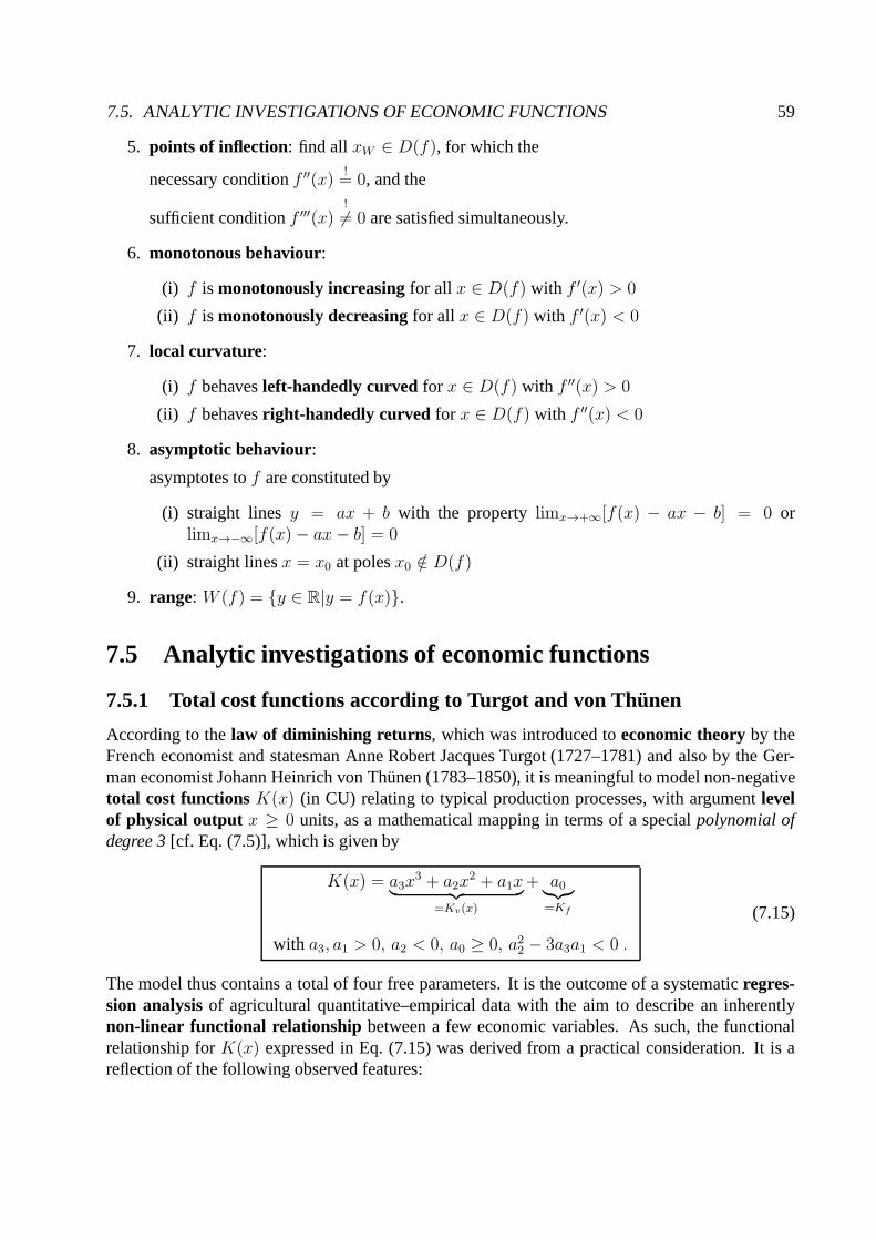
http://www.nobelprize.org/nobel_prizes/economics/laureates/2002/

7.5. ANALYTIC INVESTIGATIONS OF ECONOMIC FUNCTIONS 59

5. points of inflection: find all xW ∈ D(f), for which the

necessary conditionf ′′(x)!= 0, and the

sufficient conditionf ′′′(x)!

6= 0 are satisfied simultaneously.

6. monotonous behaviour:

(i) f is monotonously increasingfor all x ∈ D(f) with f ′(x) > 0

(ii) f is monotonously decreasingfor all x ∈ D(f) with f ′(x) < 0

7. local curvature:

(i) f behavesleft-handedly curved for x ∈ D(f) with f ′′(x) > 0

(ii) f behavesright-handedly curved for x ∈ D(f) with f ′′(x) < 0

8. asymptotic behaviour:

asymptotes tof are constituted by

(i) straight linesy = ax + b with the propertylimx→+∞[f(x) − ax − b] = 0 orlimx→−∞[f(x)− ax− b] = 0

(ii) straight linesx = x0 at polesx0 /∈ D(f)

9. range: W (f) = {y ∈ R|y = f(x)}.

7.5 Analytic investigations of economic functions

7.5.1 Total cost functions according to Turgot and von Thunen

According to thelaw of diminishing returns , which was introduced toeconomic theoryby theFrench economist and statesman Anne Robert Jacques Turgot (1727–1781) and also by the Ger-man economist Johann Heinrich von Thunen (1783–1850), it is meaningful to model non-negativetotal cost functionsK(x) (in CU) relating to typical production processes, with argument levelof physical output x ≥ 0 units, as a mathematical mapping in terms of a specialpolynomial ofdegree 3[cf. Eq. (7.5)], which is given by

K(x) = a3x3 + a2x

2 + a1x︸︷︷︸

=Kv(x)

+ a0︸︷︷︸

=Kf

with a3, a1 > 0, a2 < 0, a0 ≥ 0, a22 − 3a3a1 < 0 .

(7.15)

The model thus contains a total of four free parameters. It isthe outcome of a systematicregres-sion analysisof agricultural quantitative–empirical data with the aim to describe an inherentlynon-linear functional relationship between a few economic variables. As such, the functionalrelationship forK(x) expressed in Eq. (7.15) was derived from a practical consideration. It is areflection of the following observed features:

http://en.wikipedia.org/wiki/Anne-Robert-Jacques_Turgot,_Baron_de_Laune

http://en.wikipedia.org/wiki/Johann_Heinrich_von_Th�nen


(i) for levels of physical outputx ≥ 0 units, the total costs relating to typical productionprocesses exhibit strictly monotonously increasing behaviour; thus

(ii) for the total costs there donot exist neither roots nor local extremal values;2 however,

(iii) the total costs displayexactly onepoint of inflection.

The continuous curve forK(x) resulting from these considerations exhibits the characteristic shapeof an inverted capital letter “S”: beginning at a positive value corresponding to fixed costs, the totalcosts first increase degressively up to a point of inflection,whereafter they continue to increase,but in a progressive fashion.

In broad terms, the functional expression given in Eq. (7.15) to model totals costs in dependenceof the level of physical output is the sum of two contributions, thevariable costsKv(x) and thefixed costsKf = a0, viz.

K(x) = Kv(x) +Kf . (7.16)

In economic theory, it is commonplace to partitiontotal cost functionsin the diminishing returnspicture intofour phases, the boundaries of which are designated by special values ofthe level ofphysical output of a production process:

• phase I(interval0 units≤ x ≤ xW ):

the total costsK(x) possess at a level of physical outputxW = −a2/(3a3) > 0 units apoint of inflection. For values ofx smaller thanxW , one obtainsK ′′(x) < 0 CU/unit2, i.e.,K(x) increases in a degressive fashion. For values ofx larger thanxW , the opposite applies,K ′′(x) > 0 CU/unit2, i.e.,K(x) increases in a progressive fashion. Themarginal costs,given by

K ′(x) = 3a3x2 + 2a2x+ a1 > 0 CU/unit for all x ≥ 0 units, (7.17)

attain aminimum at the same level of physical output,xW = −a2/(3a3).

• phase II (intervalxW < x ≤ xg1):

thevariable average costs

Kv(x)

x= a3x

2 + a2x+ a1 , x > 0 units (7.18)

becomeminimal at a level of physical outputxg1 = −a2/(2a3) > 0 units. At this valueof x, equality of variable average costs and marginal costsapplies, i.e.,

Kv(x)

x= K ′(x) , (7.19)

2The last condition in Eq. (7.15) ensures a first derivative ofK(x) that doesnot possess any roots; cf. the case of

a quadratic algebraic equation0!= ax2 + bx+ c, with discriminantb2 − 4ac < 0.


which follows by the quotient rule of differentiation from the necessary condition for anextremum of the variable average costs,

0!=

(Kv(x)

x

)′

=(K(x)−Kf )

′ · x−Kv(x) · 1x2

,

and the fact thatK ′f = 0 CU/unit. Taking care of the equality (7.19), one finds for thetangent

toK(x) in the point(xg1 , K(xg1)) the equation [cf. Eq. (7.13)]

T (x) = K(xg1)+K ′(xg1)(x−xg1) = Kv(xg1)+Kf+Kv(xg1)

xg1

(x−xg1) = Kf+Kv(xg1)

xg1

x .

Its intercept with theK-axis is atKf .

• phase III (intervalxg1 < x ≤ xg2):

Theaverage costs

K(x)

x= a3x

2 + a2x+ a1 +a0x

, x > 0 units (7.20)

attain aminimum at a level of physical outputxg2 > 0 units, the defining equation of which

is given by0 CU!= 2a3x

3g2 + a2x

2g2 − a0. At this value ofx, equality of average costs and

marginal costsobtains, viz.K(x)

x= K ′(x) , (7.21)

which follows by the quotient rule of differentiation from the necessary condition for anextremum of the average costs,

0!=

(K(x)

x

)′

=K ′(x) · x−K(x) · 1

x2.

Since a quotient can be zero only when its numerator vanishes(and its denominator remainsnon-zero), one finds from re-arranging the numerator expression equated to zero the property

K ′(x)

K(x)/x= x

K ′(x)

K(x)= 1 for x = xg2 . (7.22)

The corresponding extremal value pair(xg2, K(xg2)) is referred to ineconomic theoryas theminimum efficient scale (MES). From a business economics perspective, at a level of phys-ical outputx = xg2 the (compared to our remarks in the Introduction inverted) ratio “INPUT

over OUTPUT,” i.e.,K(x)

x, becomes most favourable. By respecting the property (7.21),

the equation for the tangent toK(x) in this point [cf. Eq. (7.13)] becomes

T (x) = K(xg2) +K ′(xg2)(x− xg2) = K(xg2) +K(xg2)

xg2

(x− xg2) =K(xg2)

xg2

x .

Its intercept with theK-axis is thus at0 CU.


• phase IV (half-intervalx > xg2):

In this phaseK ′(x)/K(x)/x > 1 obtains; the costs associated with the production of oneadditional unit of a good, approximately the marginal costsK ′(x), now exceed the aver-age costs,K(x)/x. This situation is considered unfavourable from a businesseconomicsperspective.

7.5.2 Profit functions in the diminishing returns picture

In this section, we confine our considerations, for reasons of simplicity, to a market sitution withonly a single supplier of a good in demand. The price policy that this single supplier may thusinact defines a state ofmonopoly. Moreover, in addition we want toassumethat for the marketsituation consideredeconomic equilibrium obtains. This manifests itself in equality ofsupplyanddemand, viz.

x(p) = N(p) , (7.23)

whereinx denotes a non-negativesupply function (in units) (which is synonymous with the sup-plier’s level of physical output) andN a non-negativedemand function (in units), both of whichare taken to depend on the positiveunit price p (in CU/unit) of the good in question. Thesupplyfunction, and with it theunit price , can, of course, be prescribed by the monopolistic supplierinan arbitrary fashion. In a specific quantitative economic model, for instance, thedemand func-tion x(p) (recall that by Eq. (7.23)x(p) = N(p) obtains) could be assumed to be either a linear ora quadratic function ofp. In any case, in order forx(p) to realistically describe an actual demand–unit price relationship, it should be chosen as a strictly monotonously decreasing function, and assuch it isinvertible. The non-negativedemand function x(p) features two characteristic points,signified by its intercepts with thex- and thep-axes. Theprohibitive price pproh is to be deter-

mined from the conditionx(pproh)!= 0 units; therefore, it constitutes a root ofx(p). Thesaturation

quantity xsat, on the other hand, is defined byxsat := x(0 CU/unit).

The inverse function associated with the strictly monotonously decreasing non-negativedemandfunction x(p), the unit price function p(x) (in CU/unit), is likewise strictly monotonouslydecreasing. Viap(x), one calculates, in dependence on a known amountx of units sup-plied/demanded (i.e., sold), thetotal revenue (in CU) made by a monopolist according to (cf.Sec. 7.3)

E(x) = xp(x) . (7.24)

Under theassumptionthat the non-negativetotal costsK(x) (in CU) underlying the productionprocess of the good in demand can be modelled according to thediminishing returns picture ofTurgot and von Thunen, theprofit function (in CU) of the monopolist in dependence on the levelof physical output takes the form

G(x) = E(x)−K(x) = x

unit price︷︸︸︷

p(x)︸︷︷︸

total revenue

−[a3x

3 + a2x2 + a1x+ a0

]

︸︷︷︸

total costs

. (7.25)


The first two derivatives ofG(x) with respect to its argumentx are given by

G′(x) = E ′(x)−K ′(x) = xp′(x) + p(x)−[3a3x

2 + 2a2x+ a1]

(7.26)

G′′(x) = E ′′(x)−K ′′(x) = xp′′(x) + 2p′(x)− [6a3x+ 2a2] . (7.27)

Employing the principles of curve sketching set out in Sec. 7.4, the following characteristic valuesof G(x) can thus be identified:

• break-even point

xS > 0 units, as the unique solution to the conditions

G(x)!= 0 CU (necessary condition) (7.28)

andG′(x)

!> 0 CU/unit (sufficient condition), (7.29)

• end of the profitable zone

xG > 0 units, as the unique solution to the conditions

G(x)!= 0 CU (necessary condition) (7.30)

andG′(x)

!< 0 CU/unit (sufficient condition), (7.31)

• maximum profit

xM > 0 CU, as the unique solution to the conditions

G′(x)!= 0 CU/unit (necessary condition) (7.32)

andG′′(x)

!< 0 CU/unit2 (sufficient condition). (7.33)

At this point, we like to draw the reader’s attention to a special geometric property of the quan-titative model forprofit that we just have outlined: at maximum profit, thetotal revenue func-tion E(x) and thetotal cost function K(x) always possessparallel tangents. This is due to thefact that by the necessary condition for an extremum to exist, one finds that

0 CU/unit!= G′(x) = E ′(x)−K ′(x) ⇔ E ′(x)

!= K ′(x) . (7.34)

GDC: Roots and local maxima resp. minima can be easily determinedfor a given stored functionin modeCALC by employing the interactive routineszero andmaximum resp.minimum.

To conclude these considerations, we briefly turn to elucidate the technical termCournot’s point ,which frequently arises in quantitative discussions ineconomic theory; this is named after theFrench mathematician and economist Antoine–Augustin Cournot (1801–1877).Cournot’s point

http://turnbull.mcs.st-and.ac.uk/history/Biographies/Cournot.html


simply labels the profit-optimal combination of the level ofphysical output and the associated unitprice,(xM , p(xM)), for theunit price function p(x) of a good in a monopolistic market situation.Note that for this specific combination of optimal values theAmoroso–Robinson formulaapplies,which was developed by the Italian mathematician and economist Luigi Amoroso (1886–1965)and the British economist Joan Violet Robinson (1903–1983). This states that

p(xM ) =K ′(xM)

1 + εp(xM), (7.35)

with K ′(xM) the value of the marginal costs atxM , andεp(xM) the value of theelasticity of theunit price function atxM (see the following Sec. 7.6). Starting from the defining equation of thetotal revenueE(x) = xp(x), theAmoroso–Robinson formulais derived by evaluating the firstderivative ofE(x) atxM , so

E ′(xM) = p(xM) + xMp′(xM ) = p(xM)

[

1 + xMp′(xM )

p(xM)

] Sec. 7.6︷︸︸︷= = p(xM) [1 + εp(xM )] ,

and then re-arranging to solve forp(xM), using the fact thatE ′(xM ) = K ′(xM).

Remark: In a market situation whereperfect competition applies, oneassumesthat theunitprice function has settled to aconstantvaluep(x) = p = constant> 0 CU/unit (and, hence,p′(x) = 0 CU/unit2 obtains).

7.5.3 Extremal values of rational economic functions

Now we want to address the determination of extremal values of economic functions that constituteratios in the sense of the construction

OUTPUTINPUT

,

a topic raised in the Introduction.

Let us consider two examples for determininglocal maximaof ratios of this kind.

(i) We begin with theaverage profit in dependence on the level of physical outputx ≥ 0 units,

G(x)

x. (7.36)

The conditions that determine a local maximum are[G(x)/x]′!= 0 CU/unit2 and

[G(x)/x]′′!< 0 CU/unit3. Respecting the quotient rule of differentiation (cf. Sec.7.2),

the first condition yieldsG′(x)x−G(x)

x2= 0 GE/ME2 . (7.37)

Since a quotient can only be zero when its numerator vanisheswhile its denominator remainsnon-zero, it immediately follows that

G′(x)x−G(x) = 0 CU ⇒ xG′(x)

G(x)= 1 . (7.38)

http://en.wikipedia.org/wiki/Luigi_Amoroso

http://en.wikipedia.org/wiki/Joan_Robinson

7.6. ELASTICITIES 65

The task at hand now is to find a (unique) value of the level of physical outputx whichsatisfies this last condition, and for which the second derivative of the average profit becomesnegative.

(ii) To compare the performance of two companies over a givenperiod of time in a meaningfulway, it is recommended to adhere only to measures that aredimensionless ratios, and soindependent ofscale. An example of such a dimensionless ratio is the measure referred toaseconomic efficiency,

W (x) =E(x)

K(x), (7.39)

which expresses thetotal revenue(in CU) of a company for a given period as a multiple ofthe total costs(in CU) it had to endure during this period, both as functionsof the level ofphysical output. In analogy to our discussion in (i), the conditions for the existence of a

local maximum amount to[E(x)/K(x)]′!= 0 × 1/unit and[E(x)/K(x)]′′

!< 0 × 1/unit2.

By the quotient rule of differentiation (see Sec. 7.2), the first condition leads to

E ′(x)K(x)−E(x)K ′(x)

K2(x)= 0× 1/unit , (7.40)

i.e., forK(x) > 0 CU,

E ′(x)K(x)−E(x)K ′(x) = 0 CU2/unit . (7.41)

By re-arranging and multiplication withx > 0 unit, this can be cast into the particular form

xE ′(x)

E(x)= x

K ′(x)

K(x). (7.42)

The reason for this special kind of representation of the necessary condition for a localmaximum to exist [and also for Eq. (7.38)] will be clarified inthe subsequent section. Again,a value of the level of physical output which satisfies Eq. (7.42) must in addition lead toa negative second derivative of theeconomic efficiencyin order to satisfy the sufficientcondition for a local maximum to exist.

7.6 Elasticities

Finally, we pick up once more the discussion on quantifying the local variability of differentiablereal-valued functions of one real variable,f : D ⊆ R → W ⊆ R, though from a slightly differentperspective. For reasons to be elucidated shortly, we confine ourselves to considerations of regimesof f with positivevalues of the argumentx and alsopositivevaluesy = f(x) > 0 of the functionitself.

As before in Sec. 7.2, we want to assume a small change of the value of the argumentx andevaluate its resultant effect on the valuey = f(x). This yields

x∆x∈R−→ x+∆x =⇒ y = f(x)

∆y∈R−→ y +∆y = f(x+∆x) . (7.43)


We remark in passing thatrelative changesof non-negative quantities are defined by the quotient

new value− old valueold value

under the prerequisite that “old value> 0” applies. It follows from this specific construction thatthe minimum value a relative change can possibly attain amounts to “−1” (corresponding to adecrease of the “old value” by 100%).

Related to this consideration we identify the following terms:

• a prescribedabsolute changeof the independent variablex: ∆x ,

• the resultantabsolute changeof the functionf : ∆y = f(x+∆x)− f(x) ,

• the associatedrelative changeof the independent variablex:∆x

x,

• the associated resultantrelative changeof the functionf :∆y

y=

f(x+∆x)− f(x)

f(x).

Now let us compare theorder-of-magnitudesof the two relative changes just envisaged,∆x

xand

∆y

y. This is realised by considering the value of their quotient, “resultant relative change off

divided by the prescribed relative change ofx”’:

∆y

y∆x

x

=

f(x+∆x)− f(x)

f(x)∆x

x

.

Since we assumedf to be differentiable, it is possible to investigate the behaviour of this quotient

of relative changes in the limit of increasingly smaller prescribed relative changes∆x

x→ 0 ⇒

∆x → 0 near somex > 0. One thus defines:

Def.: For a differentiable real-valued functionf of one real variablex, the dimensionless(i.e.,units-independent) quantity

εf(x) := lim∆x→0

∆y

y∆x

x

= lim∆x→0

f(x+∆x)− f(x)

f(x)∆x

x

= xf ′(x)

f(x)(7.44)

is referred to as theelasticity of the functionf at positionx.

The elasticity off quantifies its resultant relative change in response to a prescribed infinitesimallysmall relative change of its argumentx, starting from some positive initial valuex > 0. As such itconstitutes a measure for therelative local rate of changeof a functionf in a point(x, f(x)). In


economic theory, in particular, one adheres to the following interpretation of the elasticityεf(x):when the postive argumentx of some positive differentiable real-valued functionf is increased by1 %, then in consequencef will change approximately byεf(x)× 1 %.

In the scientific literature one often finds the elasticity ofa positive differentiable functionf of apositive argumentx expressed in terms of logarithmic differentiation. That is,

εf(x) :=d ln[f(x)]

d ln(x)for x > 0 andf(x) > 0 ,

since by the chain rule of differentiation it holds that

d ln[f(x)]

d ln(x)=

df(x)

f(x)dx

x

= x

df(x)

dxf(x)

= xf ′(x)

f(x).

The logarithmic representation of the elasticity of a differentiable functionf immediately explainswhy, at the beginning, we confined our considerations to positive differentiable functions of posi-tive arguments only.3 A brief look at the list of standard economic functions provided in Sec. 7.3reveals that most of these (though not all) are positive functions of non-negative arguments.

For the elementary classes of real-valued functions of one real variable discussed in Sec. 7.1 onefinds:

Standard elasticities

1. f(x) = xn for n ∈ N andx ∈ R>0 ⇒ εf(x) = n (natural power-law functions)

2. f(x) = xα for α ∈ R andx ∈ R>0 ⇒ εf(x) = α (general power-law functions)

3. f(x) = ax for a ∈ R>0\{1} andx ∈ R>0 ⇒ εf(x) = ln(a)x (exponential functions)

4. f(x) = eax for a ∈ R andx ∈ R>0 ⇒ εf(x) = ax (natural exponential functions)

5. f(x) = loga(x) for a ∈ R>0\{1} andx ∈ R>0

⇒ εf (x) =1

ln(a) loga(x)(logarithmic functions)

6. f(x) = ln(x) for x ∈ R>0 ⇒ εf(x) =1

ln(x)(natural logarithmic function ).

In view of these results, we would like to emphasise the fact that for the entire family ofgen-eral power-law functions the elasticityεf(x) has aconstant value, independent of the value ofthe argumentx. It is this very property which classifiesgeneral power-law functionsasscale-invariant . Whenscale-invarianceobtains, dimensionless ratios, i.e., quotients of variables of the

3To extend the regime of applicability of the measureεf , one may consider working in terms of absolute values|x|and|f(x)|. Then one has to distinguish between four cases, which need to be looked at separately: (i)x > 0, f(x) > 0,(ii) x < 0, f(x) > 0, (iii) x < 0, f(x) < 0 and (iv)x > 0, f(x) < 0.


same physical dimension, reduce toconstants. In this context, we would like to remark that scale-invariant (fractal) power-law functions of the formf(x) = Kxα, with K > 0 andα ∈ R<0\{−1},are frequently employed inEconomicsand theSocial Sciencesfor modellinguncertainty of eco-nomic agentsin decision-making processes, or for describing probability distributions ofrareevent phenomena; see, e.g., Taleb (2007) [25, p 326ff] or Gleick (1987) [13, Chs. 5 and 6]. Thisis due, in part, to the curious property that for certain values of the exponentα general power-lawprobability distributions attain unbounded variance; cf.Ref. [12, Sec. 8.9].

Practical applications ineconomic theoryof the concept of an elasticty as a measure of relativechange of a differentiable real-valued functionf of one real variablex are generally based on thefollowing linear (!) approximation: beginning atx0 > 0, for small prescribed percentage changes

of the argumentx in the interval0 % <∆x

x0≤ 5 %, the resultant percentage changes off amount

approximately to

(percentage change off) ≈ (elasticity off atx0)× (percentage change ofx) , (7.45)

or, in terms of a mathematical formula, to

f(x0 +∆x)− f(x0)

f(x0)≈ εf(x0)

∆x

x0. (7.46)

We now draw the reader’s attention to a special kind of terminology developed ineconomic theoryto describe therelative local change behaviourof economic functions in qualitative terms. Forx ∈ D(f), the relative local change behaviour of a functionf is called

• inelastic, whenever|εf(x)| < 1,

• unit elastic, when|εf(x)| = 1, and

• elastic, whenever|εf(x)| > 1.

For example, a total cost functionK(x) in the diminishing returns picture exhibits unit elasticbehaviour at the minimum efficient scalex = xg2 where, by Eq. (7.22),εK(xg2) = 1. Also, atthe local maximum of an average profit functionG(x)/x, the propertyεG(x) = 1 applies; cf.Eq. (7.38).

Next, we review the computational rules one needs to adhere to when calculating elasticities forcombinations of two real-valued functions of one real variable in the sense of Sec. 7.1.6:

Computational rules for elasticitiesIf f andg are differentiable real-valued functions of one real variable, with elasticitiesεf andεg,it holds that:

1. product f · g: εf ·g(x) = εf(x) + εg(x),

2. quotientf

g, g 6= 0: εf/g(x) = εf(x)− εg(x),

3. concatenationf ◦ g: εf◦g(x) = εf(g(x)) · εg(x),


4. inverse functionf−1: εf−1(x) =1

εf (y)

∣∣∣∣y=f−1(x)

.

To end this chapter, we remark that for a positive differentiable real-valued functionf of onepositive real variablex, a second elasticity may be defined according to

εf [εf(x)] := xd

dx

[x

f(x)

df(x)

dx

]

. (7.47)

Of course, by analogy this procedure may be generalised to higher derivatives off still.

Chapter 8

Integral calculus of real-valued functions ofone real variable

In the final chapter of these lecture notes we give a brief overview of the main definitions andlaws of theintegral calculus of real-valued functions of one variable. Subsequently we considera simple application of this tool ineconomic theory.

8.1 Indefinite integrals

Def.: Let f be a continuous real-valued function of one real variable and F a differentiable real-valued function of the same real variable, withD(f) = D(F ). Given thatf andF are relatedaccording to

F ′(x) = f(x) for all x ∈ D(f) , (8.1)

thenF is referred to as aprimitive of f .

Remark: The primitive of a given continuous real-valued functionf cannotbe unique. By therules of differentiation discussed in Sec. 7.2, besidesF alsoF + c, with c ∈ R a real-valuedconstant, constitutes a primitive off since(c)′ = 0.

Def.: If F is a primitive of a continuous real-valued functionf of one real variable, then

∫

f(x) dx = F (x) + c , c = constant∈ R , with F ′(x) = f(x) (8.2)

defines theindefinite integral of the functionf . The following names are used to refer to thedifferent ingredients in this expression:

• x — the integration variable,

• f(x) — the integrand,

• dx — thedifferential , and, lastly,

71

72 CHAPTER 8. INTEGRAL CALCULUS OF REAL-VALUED FUNCTIONS

• c — theconstant of integration.

For the elementary, continuous real-valued functions of one variable introduced in Sec. 7.1, thefollowing rules of indefinite integration apply:

Rules of indefinite integration

1.∫α dx = αx+ c with α = constant∈ R (constants)

2.∫

x dx =x2

2+ c (linear functions)

3.∫

xn dx =xn+1

n+ 1+ c for n ∈ N (natural power-law functions)

4.∫

xα dx =xα+1

α + 1+ c for α ∈ R\{−1} andx ∈ R>0 (general power-law functions)

5.∫

ax dx =ax

ln(a)+ c for a ∈ R>0\{1} (exponential functions)

6.∫

eax dx =eax

a+ c for a ∈ R\{0} (natural exponential functions)

7.∫x−1 dx = ln |x|+ c for x ∈ R\{0}.

Special methods of integration need to be employed when the integrand consists of a concatanationof elementary real-valued functions. Here we provide a listwith the main tools for this purpose.For differentiable real-valued functionsf andg, it holds that

1.∫(αf(x)± βg(x)) dx = α

∫f(x) dx± β

∫g(x) dx

with α, β = constant∈ R (summation rule)

2.∫f(x)g′(x) dx = f(x)g(x)−

∫f ′(x)g(x) dx (integration by parts)

3.∫f(g(x))g′(x) dx

u=g(x) anddu=g′(x)dx︷︸︸︷=

∫f(u) du = F (g(x)) + c (substitution method)

4.∫

f ′(x)

f(x)dx = ln |f(x)|+ c for f(x) 6= 0 (logarithmic integration ).

8.2 Definite integrals

Def.: Let f be a real-valued function of one variable which is continuous on an interval[a, b] ⊂D(f), and letF be a primitive off . Then the expression

∫ b

a

f(x) dx = F (x)|x=bx=a = F (b)− F (a) (8.3)

defines thedefinite integral of f in the limits of integration a andb.

For definite integrals the following general rules apply:

8.3. APPLICATIONS IN ECONOMIC THEORY 73

1.∫ a

a

f(x) dx = 0 (identical limits of integration )

2.∫ a

b

f(x) dx = −∫ b

a

f(x) dx (interchange of limits of integration)

3.∫ b

a

f(x) dx =

∫ c

a

f(x) dx+

∫ b

c

f(x) dx for c ∈ [a, b] (split of integration interval ).

Remark: The main qualitative difference between an (i) indefinite integral and a (ii) definite in-tegral of a continuous real-valued function of one variablereveals intself in the different kinds ofoutcome: while (i) yields as a result a real-valued (primitive) function, (ii) simply yields a singlerealnumber.

GDC: For a stored real-valued function, the evaluation of a definite integral can be performed inmodeCALCwith the pre-programmed function

∫f(x)dx. The corresponding limits of integration

need to be specified interactively.

As indicated in Sec. 7.6, the scale-invariant power-law functions f(x) = xα for α ∈ R andx ∈ R>0 play a special role in practical applications. Forx ∈ [a, b] ⊂ R>0 andα 6= −1 it holdsthat

∫ b

a

xα dx =xα+1

α+ 1

∣∣∣∣

x=b

x=a

=1

α + 1

(bα+1 − aα+1

). (8.4)

Problematic in this context can be considerations of takinglimits of the forma → 0 resp.b → ∞,since for either of the two cases

(i) caseα < −1:

lima→0

∫ b

a

xα dx → ∞ , (8.5)

(ii) caseα > −1:

limb→∞

∫ b

a

xα dx → ∞ , (8.6)

one ends up withdivergent mathematical expressions.

8.3 Applications in economic theory

The starting point shall be a simple market situation for a single product. For this product, on theone-hand side, there be ademand functionN(p) (in units) which is monotonously decreasing onthe price interval[pu, po]; the limit valuespu andpo denote the minimum and maximum prices perunit (in CU/u) acceptable for the product. On the other hand,the market situation be described byasupply function A(p) (in units) which is monotonously increasing on[pu, po].

The equilibrium unit price pM (in CU/unit) for this product is defined by assuming a state ofeconomic equilibrium of the market, quantitatively expressed by the condition

A(pM) = N(pM) . (8.7)

74 CHAPTER 8. INTEGRAL CALCULUS OF REAL-VALUED FUNCTIONS

Geometrically, this condition defines common points of intersection for the functionsA(p) andN(p) (when they exist).

GDC: Common points of intersection for stored functionsf andg can be easily determined inter-actively in modeCALC employing the routineintersect.

In a drastically simplified fashion, we now turn to compute the revenue made on the market by thesuppliers of a new product for either of three possiblestrategies of market entry.

1. Strategy 1: The revenue obtained by the suppliers when the new product isbeing soldstraight at the equilibrium unit pricepM , in an amountN(pM), is simply given by

U1 = U(pM ) = pMN(pM) (in CU) . (8.8)

2. Strategy 2: Some consumers would be willing to purchase the product intially also at a unitprice which is higher thanpM . If, hence, the suppliers decide to offer the product initiallyat a unit pricepo > pM , and then, in order to generate further demand, to continuously1 (!)reducethe unit price to the lowerpM , the revenue obtained yields the larger value

U2 = U(pM ) +

∫ po

pM

N(p) dp . (8.9)

Since the amount of money

K :=

∫ po

pM

N(p) dp (in CU) (8.10)

is (theoretically) safed by the consumers when the product is introduced to the market ac-cording to strategy 1, this amount is referred to in the economic literature asconsumersurplus.

3. Strategy 3: Some suppliers would be willing to introduce the product to the market initiallyat a unit price which is lower thanpM . If, hence, the suppliers decide to offer the productinitially at a unit pricepu < pM , and then to continuously2 (!) raise it to the higherpM , therevenue obtaines amounts to the smaller value

U3 = U(pM)−∫ pM

pu

A(p) dp . (8.11)

Since the suppliers (theoretically) earn the extra amount

P :=

∫ pM

pu

A(p) dp (in CU) (8.12)

when the product is introduced to the market according to strategy 1, this amount is referredto in the economic literature asproducer surplus.

1This is a strong mathematical assumption aimed at facilitating the actual calculation to follow.2See previous footnote.

Appendix A

Glossary of technical terms (GB – D)

Aabsolute change: absoluteAnderungabsolute value: Betragaccount balance: Kontostandaddition: Additionanalysis: Analysis, Untersuchung auf Differenzierbarkeitseigenschaftenarithmetical mean: arithmetischer Mittelwertarithmetical sequence: arithmetische Zahlenfolgearithmetical series: arithmetische Reiheaugmented coefficient matrix: erweiterte Koeffizientenmatrixaverage costs: Stuckkostenaverage profit: Durchschnittsgewinn, Gewinn pro Stuck

Bbackward substitution: ruckwertige Substitutionbalance equation: Bilanzgleichungbasis: Basisbasis solution: Basislosungbasis variable: BasisvariableBehavioural Economics: Verhaltensokonomikboundary condition: Randbedingungbreak-even point: Gewinnschwelle

Cchain rule: Kettenregelcharacteristic equation: charakteristische Gleichungcoefficient matrix: Koeffizientenmatrixcolumn: Spaltecolumn vector: Spaltenvektorcomponent: Komponentecompound interest: Zinseszinsconcatenation: Verschachtelung, Verknupfungconservation law: Erhaltungssatz

75

76 APPENDIX A. GLOSSARY OF TECHNICAL TERMS (GB – D)

constant of integration: Integrationskonstanteconstraint: Zwangsbedingungcost function: Kostenfunktionconsumer surplus: Konsumentenrentecontinuity: Stetigkeitcontract period: LaufzeitCournot’s point: Cournotscher Punktcurve sketching: Kurvendiskussion

Ddecision-making: Entscheidungsfindungdeclining-balance depreciation method: geometrisch–degressive Abschreibungdefinite integral: bestimmtes Integraldemand function: Nachfragefunktiondependent variable: abhangige Variabledepreciation: Abschreibungdepreciation factor: Abschreibungsfaktorderivative: Ableitungdeterminant: Determinantedifference: Differenzdifference quotient: Differenzenquotientdifferentiable: differenzierbardifferential: Integrationsdifferenzialdifferential calculus: Differenzialrechnungdimension: Dimensiondirection of optimisation: Optimierungsrichtungdivergent: divergent, unbeschr”anktdomain: Definitionsbereich

Eeconomic agent: Wirtschaftstreibende(r) (meistens einhomo oeconomicus)economic efficiency: Wirtschaftlichkeiteconomic equilibrium: okonomisches Gleichgewichteconomic principle: okonomisches Prinzipeconomic theory: WirtschaftstheorieEconophysics:Okonophysikeigenvalue: Eigenwerteigenvector: Eigenvektorelastic: elastischelasticity: Elastizitatelement: Elementend of profitable zone: Gewinngrenzeendogenous: endogenequilibrium price: Marktpreisequivalence transformation:Aquivalenztransformation

77

exogenous: exogenexponential function: Exponentialfunktionextrapolation: Extrapolation, uber bekannten Gutigkeitsbereich hinaus verallgemeinern

Ffeasible region: zulassiger Bereichfinal capital: Endkapitalfixed costs: Fixkostenforecasting: Vorhersagen erstellenfunction: Funktion

GGaußian elimination: Gauß’scher AlgorithmusGDC: GTR, grafikfahiger Taschenrechnergeometrical mean: geometrischer Mittelwertgeometrical sequence: geometrische Zahlenfolgegeometrical series: geometrische Reihegrowth function: Wachstumsfunktion

H

Iidentity: Identitatimage vector: Absolutgliedvektorindefinite integral: unbestimmtes Integralindependent variable: unabhangige Variableinelastic: unelastischinitial capital: Anfangskapitalinstallment: Ratenzahlunginstallment savings: Ratensparenintegral calculus: Integralrechnungintegrand: Integrandintegration variable: Integrationsvariableinterest factor: Aufzinsfaktorinterest rate: Zinsfußinverse function: Inversfunktion, Umkehrfunktioninverse matrix: inverse Matrix, Umkehrmatrixisoquant: Isoquante

J

K

Llaw of diminishing returns: Ertragsgesetz


length: Langelevel of physical output: Ausbringungsmengelimits of integration: Integrationsgrenzenlinear combination: Linearkombinationlinearisation: Linearisierunglinear programming: lineare Optimierunglocal rate of change: lokaleAnderungsratelogarithmic function: Logarithmusfunktion

Mmapping: Abbildungmarginal costs: Grenzkostenmaximisation: Maximierungminimisation: Minimierungminimum efficient scale: Betriebsoptimummonetary value: Geldwertmonopoly: Monopolmonotonicity: Monotoniemortgage loan: Darlehen

Nnon-basis variable: Nichtbasisvariablenon-negativity constraints: Nichtnegativitatsbedingungennon-linear functional relationship: nichtlineare Funktionalbeziehung

Oobjective function: Zielfunktionone-to-one and onto: eineindeutigoptimal solution: optimalen Losungoptimal value: optimaler Wertoptimisation: Optimierungorder-of-magnitude: Großenordnungorthogonal: orthogonalover-determined: uberbestimmt

Pparallel displacement: Parallelverschiebungpension calculations: Rentenrechnungpercentage rate: Prozentsatzperfect competition: totale Konkurrenzperiod: Periodepivot column index: Pivotspaltenindexpivot element: Pivotelementpivot operation: Pivotschrittpivot row index: Pivotzeilenindexpole: Polstelle, Singularitatpolynomial division: Polynomdivision

79

polynomial of degreen: Polynom vom Gradnpower-law function: Potenzfunktionpresent value: Barwertprimitive: Stammfunktionprincipal component analysis: Hauptkomponentenanalyseproducer surplus: Produzentenrenteproduct rule: Produktregelprofit function: Gewinnfunktionprohibitive price: PohibitivpreisProspect Theory: Neue Erwartungstheoriepsychological value function: psychologische Wertfunktion

Qquadratic matrix: quadratische Matrixquotient: Quotientquotient rule: Quotientenregel

Rrange: Wertespektrumrank: Rangrare event: seltenes Ereignisrational function: gebrochen rationale Funktionreal-valued function: reellwertige Funktionreference period: Referenzzeitraumregression analysis: Regressionsanalyseregular: regularrelative change: relativeAnderungremaining debt: Restschuldremaining resources: Restkapazitatenremaining value: Restwertrescaling: Skalierungresources: Rohstofferesource consumption matrix: Rohstoffverbrauchsmatrixrestrictions: Restriktionenroot: Nullstellerow: Reiherow vector: Zeilenvektor

Ssaturation quantity: Sattigungsmengescale: Skala, Großenordnungscale-invariant: skaleninvariantsimplex: Simplex, konvexer Polyedersimplex tableau: Simplextabellesingular: singularsink: Senke


slack variable: Schlupfvariablesource: Quellestationary: stationar, konstant in der Zeitstraight line depreciation method: lineare Abschreibungstrictly monotonously decreasing: streng monoton fallendstrictly monotonously increasing: streng monoton steigendsummation rule: Summationsregelsupply function: Angebotsfunktion

Ttangent: Tangentetarget space: Wertebereichtechnology matrix: Technologiematrixtotal demand matrix: Gesamtbedarfsmatrixtotal revenue: Ertragtranspose: Transponierte

Uuncertainty: Unsicherheitunder-determined: unterbestimmtuniqueness: Eindeutigkeitunit elastic: proportional elastischunit matrix: Einheitsmatrixunit price: Stuckpreisunit vector: Einheitsvektorutility function: Nutzenfunktion

Vvalue chain: Wertschopfungskettevariability: Anderungsverhalten, Variabilitatvariable average costs: variable Stuckkostenvariable costs: variable Kostenvariable vector: Variablenvektorvector: Vektorvector algebra: Vektoralgebra

Wwell-determined: wohlbestimmt

Zzero matrix: Nullmatrixzero vector: Nullvektor

Bibliography

[1] T Arens, F Hettlich, C Karpfinger, U Kockelkorn, K Lichtenegger and H Stachel (2008)Mathematik1st Edition (Heidelberg: Spektrum) ISBN–13: 9783827417589

[2] A Asano (2013)An Introduction to Mathematics for Economics(Cambridge: CambridgeUniversity Press) ISBN–13: 9780521189460

[3] C Bauer, M Clausen, A Kerber and H Meier–Reinhold (2008)Mathematik fur Wirtschaftswis-senschaftler5th Edition (Stuttgart: Schaffer–Poeschel) ISBN–13: 9783791027487

[4] Bernoulli D (1738) Specimen theoriae novae de mensura sortis Papers of the ImperialAcademy of Sciences in St. PetersburgEnglish translation: (1954) Exposition of a new theory on the measurement of riskEconometrica2223–36

[5] J–P Bouchaud and M Potters (2003)Theory of Financial Risk and Derivative Pricing2nd

Edition (Cambridge: Cambridge University Press) ISBN–13:9780521741866

[6] K Bosch (2003)Mathematik fur Wirtschaftswissenschaftler14th Edition (Munchen: Olden-bourg) ISBN–10: 3486273094

[7] I N Bronstein, K A Semedjajew, G Musiol and H Muhlig (2005) Taschenbuch der Mathematik6th Edition (Frankfurt (Main): Harri Deutsch) ISBN–10: 3817120060

[8] G B Dantzig (1949) Programming of interdependent activities: II mathematical modelEconometrica17200–211

[9] G B Dantzig (1955) Linear programming under uncertaintyManagement Science1 197–206

[10] E T Dowling (1990)Schaum’s Outline of Calculus for Business, Economics, and the SocialSciences(New York: McGraw–Hill) ISBN–13: 9780070176737

[11] E T Dowling (2009)Schaum’s Outline of Mathematical Methods for Business and Economics(New York: McGraw–Hill) ISBN–13: 9780071635325

[12] H van Elst (2015) Foundations of descriptive and inferential statistics PreprintarXiv:1302.2525v3 [stat.AP]

[13] J Gleick (1987)Chaos — Making a New Sciencenth Edition 1998 (London: Vintage) ISBN–13: 9780749386061

81

http://www.jstor.org/stable/1909829

http://dx.doi.org/10.2307/1905523

http://dx.doi.org/10.1287/mnsc.1.3-4.197


82 BIBLIOGRAPHY

[14] J F Hair jr, W C Black, B J Babin and R E Anderson (2010)Multivariate Data Analysis7th

Edition (Upper Saddle River (NJ): Pearson) ISBN–13: 9780135153093

[15] F Herrmann (2003)Physik III: Thermodynamik — Skripten zur Experimentalphysik Univer-sitat Karlsruhe (TH) URL (cited on August 30, 2015):www.physikdidaktik.uni-karlsruhe.de/skripten/thermod.pdf

[16] J Hulsmann, W Gamerith, U Leopold–Wildburger and W Steindl (2005)Einfuhrung in dieWirtschaftsmathematik4th Edition (Berlin: Springer) ISBN–10: 3540244093

[17] D Kahneman (2011)Thinking, Fast and Slow(London: Penguin) ISBN–13: 9780141033570

[18] D Kahneman and A Tversky (1979) Prospect theory: an analysis of decision under riskEconometrica47263–292

[19] S J Leon (2009)Linear Algebra with Applications8th Edition (London: Pearson) ISBN–13:9780136009290

[20] W W Leontief (1936) Quantitative input and output relations in the economic systems of theUnited StatesThe Review of Economics and Statistics18 105–125

[21] R Penrose (2004)The Road to Reality — A Complete Guide to the Laws of the Universe1st

Edition (London: Jonathan Cape) ISBN–10: 0224044478

[22] H Rinne (2008)Taschenbuch der Statistik4th Edition (Frankfurt Main): Harri Deutsch)ISBN–13: 9783817118274

[23] S Singh (1997)Fermat’s Last Theorem(London: Fouth Estate) ISBN–13: 9781857025217

[24] L Smith (2007)Chaos — A Very Short Introduction(Oxford: Oxford University Press)ISBN–13: 9780192853783

[25] N N Taleb (2007)The Black Swan — The Impact of the Highly Improbable(London: Pen-guin) ISBN–13: 9780141034591

[26] A Zeh–Marschke (2010)Finanzmathematik — Zins und Zinseszins, Tilgungs- und Renten-rechnung, Investitionsrechnung, Abschreibungenprivate lecture notes

http://www.physikdidaktik.uni-karlsruhe.de/skripten/thermod.pdf

http://www.jstor.org/stable/1914185

http://dx.doi.org/10.2307/1927837

A INTRODUCTION TO BUSINESS MATHEMATICS … · Introduction These lecture notes contain the entire...

Documents

Transcript of A INTRODUCTION TO BUSINESS MATHEMATICS … · Introduction These lecture notes contain the entire...