A HYBRID APPROACH FOR ARTIFICIAL IMMUNE RECOGNITION SYSTEM · 2.5 Research Progress of Hybrid...
250
A HYBRID APPROACH FOR ARTIFICIAL IMMUNE RECOGNITION SYSTEM MAHMOUD REZA SAYBANI THESIS SUBMITTED IN FULFILMENT OF THE REQUIREMENTS FOR THE DEGREE OF DOCTOR OF PHILOSOPHY FACULTY OF COMPUTER SCIENCE AND INFORMATION TECHNOLOGY UNIVERSITY OF MALAYA KUALA LUMPUR 2016
Transcript of A HYBRID APPROACH FOR ARTIFICIAL IMMUNE RECOGNITION SYSTEM · 2.5 Research Progress of Hybrid...

A HYBRID APPROACH FOR ARTIFICIAL IMMUNE
RECOGNITION SYSTEM
MAHMOUD REZA SAYBANI
THESIS SUBMITTED IN FULFILMENT OF THE
REQUIREMENTS FOR THE DEGREE OF DOCTOR OF
PHILOSOPHY
FACULTY OF COMPUTER SCIENCE AND
INFORMATION TECHNOLOGY
UNIVERSITY OF MALAYA
KUALA LUMPUR
2016

ii
UNIVERSITY OF MALAYA
ORIGINAL LITERARY WORK DECLARATION
Name of Candidate: Mahmoud Reza Saybani (I.C/Passport No: L95235958)
Matric No: WHA080025
Name of Degree: Doctorate of Philosophy (PhD)
Title of Project Paper/Research Report/Dissertation/Thesis (“this Work”):
A Hybrid Approach for Artificial Immune Recognition System
Field of Study: ARTIFICIAL INTELLIGENCE
I do solemnly and sincerely declare that:
(1) I am the sole author/writer of this Work;
(2) This Work is original;
(3) Any use of any work in which copyright exists was done by way of fair dealing
and for permitted purposes and any excerpt or extract from, or reference to or
reproduction of any copyright work has been disclosed expressly and
sufficiently and the title of the Work and its authorship have been
acknowledged in this Work;
(4) I do not have any actual knowledge nor do I ought reasonably to know that the
making of this work constitutes an infringement of any copyright work;
(5) I hereby assign all and every rights in the copyright to this Work to the
University of Malaya (“UM”), who henceforth shall be owner of the copyright
in this Work and that any reproduction or use in any form or by any means
whatsoever is prohibited without the written consent of UM having been first
had and obtained;
(6) I am fully aware that if in the course of making this Work I have infringed any
copyright whether intentionally or otherwise, I may be subject to legal action
or any other action as may be determined by UM.
Candidate’s Signature Date: 08 August 2016
Subscribed and solemnly declared before,
Witness’s Signature Date:
Name:
Designation:

iii
ABSTRACT
Various data mining techniques are being used by researchers of different domains to
analyze data and extract valuable information from a data set for further use. Among all
these techniques, classification is one of the most commonly used tasks in data mining,
which is used by many researchers to classify instances into two or more pre-determined
classes. The increasing size of data being stored have created the need for computer-based
methods for automatic data analysis. Many researchers, who have developed methods and
algorithms within the field of artificial intelligence, machine learning and data mining,
have addressed extracting useful information from the data. There exist many intelligent
tools, which try to learn from the patterns in the data in order to predict classes of new
data. One of these tools is Artificial Immune Recognition System (AIRS), which has been
used increasingly. Results of AIRS have shown its potential for classification purposes.
AIRS is an intelligent classifier offering robust and powerful information processing
capabilities and is becoming steadily an effective branch of computational intelligence.
Although AIRS has shown excellent results, it still has potentials to perform even better
and deserves to be investigated. AIRS uses a linear function to determine the amount of
resources that needs to be allocated and this linearity increases the running time and thus
reduces the performance of AIRS. Resource competition part of AIRS poses another
problem, here, premature memory cells are generated and therefore classification
accuracy decreases. Further AIRS uses k-Nearest Neighbor (KNN) as a classifier and that
makes it severely vulnerable to the presence of noise, irrelevant features, and the number
of attributes. KNN uses majority voting and a drawback of this is that the classes with the
more frequent instances tend to dominate the prediction of the new instance. The
consequence of using KNN is ultimately reduction of classification accuracy.

iv
This dissertation presents the following main contributions with the goal of improving
the accuracy and performance of AIRS2. The components of the AIRS2 algorithm that
pose problems will be modified. This thesis proposes three new hybrid algorithms: The
FRA-AIRS2 algorithm uses fuzzy logic to improve data reduction capability of AIRS2
and to solve the linearity problem associated with resource allocation of AIRS. The RRC-
AIRS2 uses the concept of real-world tournament selection mechanism for controlling
the population size and improving the classification accuracy. The FSR-AIRS2 is a new
hybrid algorithm that incorporates the FRA, RRC, and the SVM into AIRS2 in order to
produce a stronger classifier. The proposed algorithms have been tested on a variety of
datasets from the UCI machine learning repository. Experimental results on real-world
machine learning benchmark data sets have demonstrated the effectiveness of the
proposed algorithms.
v
ABSTRAK
Pelbagai teknik perlombongan data telah digunakan oleh para penyelidik daripada
domain yang berbeza untuk menganalisis data dan mengekstrak maklumat yang berharga
daripada set data untuk kegunaan selanjutnya. Di antara semua teknik ini, pengelasan
adalah salah satu tugas yang paling biasa digunakan dalam perlombongan data, yang
digunakan oleh kebanyakan pengkaji untuk mengklasifikasikan instance kepada dua atau
lebih kelas yang telah ditetapkan. Peningkatan saiz data yang disimpan telah mewujudkan
keperluan bagi kaedah berasaskan komputer untuk analisis data secara automatik.
Kebanyakan penyelidik yang telah membangunkan kaedah dan algoritma dalam bidang
kepintaran buatan, pembelajaran mesin dan perlombongan data, telah mengenalpasti
maklumat yang sangat berguna daripada data. Terdapat banyak alat pintar yang wujud
yang cuba untuk belajar daripada paten dalam data untuk meramalkan kelas bagi data
yang baru. Salah satu alat pintar itu adalah Artificial Immune Recognition System (AIRS)
yang telah meningkat penggunaannya. Keputusan AIRS telah menunjukkan potensinya
untuk tujuan pengkelasan. AIRS adalah pengelas pintar yang menawarkan keupayaan
pemprosesan maklumat yang mantap dan berkuasa yang menjadi semakin berkesan untuk
kepintaran berkomputer. Walaupun AIRS telah menunjukkan hasil yang sangat baik, ia
masih mempunyai potensi untuk prestasi yang lebih baik dan wajar dikaji. AIRS
menggunakan fungsi linear untuk menentukan jumlah sumber yang perlu diperuntukkan
dan kelinearan ini meningkatkan semasa latihan dan dengan itu mengurangkan prestasi
AIRS. Sumber persaingan sebahagian daripada AIRS menimbulkan masalah lain iaitu
sel-sel memori pra-matang dihasilkan dan oleh itu ketepatan klasifikasi berkurangan.
Seterusnya AIRS menggunakan k-Nearest Neighbor (KNN) sebagai pengelas menjadikan
ia teruk terdedah kepada kehadiran bunyi, ciri-ciri yang tidak relevan, dan bilangan
atribut. KNN menggunakan undian majoriti dan kelemahannya adalah bahawa kelas-
kelas dengan instance yang lebih kerap cenderung untuk menguasai ramalan instance

vi
yang baru. Penggunaan KNN ini akhirnya mengakibatkan pengurangan ketepatan
pengelasan.
Disertasi ini membentangkan sumbangan utama yang bermatlamat untuk
meningkatkan ketepatan dan prestasi AIRS2. Komponen algoritma AIRS2 yang
menimbulkan masalah akan diubah suai. Tesis ini mencadangkan tiga algoritma hibrid
yang baru: Algoritma FRA-AIRS2 menggunakan fuzzy logic untuk meningkatkan
keupayaan pengurangan data AIRS2 dan untuk menyelesaikan masalah kelinearan yang
berkaitan dengan peruntukan sumber AIRS. RRC-AIRS2 menggunakan konsep
mekanisme pemilihan kejohanan dunia yang nyata untuk mengawal saiz penduduk dan
meningkatkan ketepatan klasifikasi. FSR-AIRS2 adalah algoritma hibrid baru yang
menggabungkan FRA, RRC, dan SVM kepada AIRS2 untuk menghasilkan pengelas yang
lebih kukuh. Algoritma yang dicadangkan telah diuji pada pelbagai set data dari gedung
UCI machine learning. Keputusan eksperimen ke atas penanda aras set data pembelajaran
mesin yang sebenar telah menunjukkan keberkesanan algoritma yang dicadangkan.

vii
ACKNOWLEDGEMENTS
I thank almighty God for providing me with all things I need, and for sustaining me
through my studies.
This work is dedicated to my mother Simin Rastegar, who passed away in 2005, my father
Ahmad Saybani, my daughter Mariam, and my brothers Mehdi, Hamidreza and Alireza
for their unconditional love, support and sacrifices.
I would like to give special thanks to my advisor Dr. Teh Ying Wah and my former co-
advisor Dr. Saeed Reza Aghabozorgi Sahaf Yazdi for their continuous encouragement,
patient guidance and support in the completion of this dissertation.
I am grateful to Dr. Shahram Golzari for all the time, patience, and the knowledge he has
imparted to me.
In no particular order, many thanks to my Austrian friends Dipl.-Ing. Erich Jank, Dipl.-
Ing. Karl Arzt, and their families, who helped knowledge and me to reach to this point of
my education, and for their moral support since 1980.
I am also thankful to my British friend Mr. Tim Challenger for his mental support and for
correcting my English mistakes.

viii
TABLE OF CONTENTS
Abstract ............................................................................................................................ iii
Abstrak .............................................................................................................................. v
Acknowledgements ......................................................................................................... vii
Table of Contents ........................................................................................................... viii
List of Figures ................................................................................................................. xii
List of Tables.................................................................................................................. xvi
List of Symbols and Abbreviations ................................................................................. xx
CHAPTER 1: INTRODUCTION .................................................................................. 1
1.1 Background and Motivation .................................................................................... 1
1.2 Research Problem .................................................................................................... 9
1.3 Research Objective ................................................................................................ 12
1.4 Research Scope ...................................................................................................... 13
1.5 Thesis Outline ........................................................................................................ 13
CHAPTER 2: LITERATURE REVIEW .................................................................... 15
2.1 Introduction............................................................................................................ 15
2.2 Classification ......................................................................................................... 15
2.3 From Human Immune System To Artificial Immune System............................... 22
2.3.1 Evolutionary Computing .......................................................................... 24
2.3.2 Common Framework ................................................................................ 29
2.3.3 Representation .......................................................................................... 31
2.3.4 Affinity Measures ..................................................................................... 31
2.3.5 Immune Algorithms ................................................................................. 32
2.4 Biologically-based Classification .......................................................................... 35
ix
2.5 Research Progress of Hybrid SVM-based Classifiers Within the AIS Domain .... 40
2.6 Artificial Immune Recognition System ................................................................. 42
2.6.1 Differences between AIRS1 and AIRS2 .................................................. 56
2.6.2 AIRS in the Literature .............................................................................. 58
2.7 Classifiers Used In This Research As Benchmark Classifiers .............................. 65
2.8 Summary ................................................................................................................ 68
CHAPTER 3: METHODOLOGY ............................................................................... 69
3.1 Introduction............................................................................................................ 69
3.2 Research Overview ................................................................................................ 69
3.3 Experimental Setup ................................................................................................ 70
3.3.1 System Specification ................................................................................ 70
3.3.2 Datasets .................................................................................................... 71
3.4 Performance and evaluation measurements........................................................... 79
3.4.1 Performance Metrics ................................................................................ 79
3.4.2 Classification accuracy ............................................................................. 79
3.4.3 N-fold cross validation ............................................................................. 80
3.4.4 Data reduction .......................................................................................... 80
3.4.5 Overall Runtime ....................................................................................... 81
3.4.6 Area under the ROC Curve the AUC ....................................................... 81
3.4.7 Student’s t test .......................................................................................... 82
3.4.8 Classification Modelling .......................................................................... 84
3.5 Well-known classifiers .......................................................................................... 84
3.6 Summary ................................................................................................................ 84
CHAPTER 4: IMPROVEMENT OF ARTIFICIAL IMMUNE RECOGNITION
SYSTEM 2 86
x
4.1 Introduction............................................................................................................ 86
4.2 Development of FRA-AIRS2 ................................................................................ 87
4.3 Development of RRC-AIRS2 ................................................................................ 97
4.3.1 Pseudocode for RRC-AIRS2 .................................................................. 102
4.4 Development of FSR-AIRS2 ............................................................................... 103
4.4.1 Pseudocode of FSR-AIRS2 .................................................................... 107
4.5 Experimental Setup .............................................................................................. 108
4.6 Results and Discussion ........................................................................................ 109
4.6.1 Evaluation of FRA-AIRS2 ..................................................................... 112
4.6.1.1 Classification Accuracy of FRA-AIRS2 versus AIRS2 .......... 112
4.6.1.2 Comparing Running Time of FRA-AIRS2 and AIRS2 on
benchmark data sets ................................................................ 117
4.6.2 Evaluation of RRC-AIRS2 ..................................................................... 119
4.6.2.1 Classification Accuracy of RRC-AIRS2 versus AIRS2 ......... 119
4.6.2.2 Comparing Running Time of RRC-AIRS2 and AIRS2 on
benchmark data sets ................................................................ 125
4.6.3 Evaluation of FSR-AIRS2 ...................................................................... 126
4.6.3.1 Classification Accuracy of FSR-AIRS2 versus AIRS2 .......... 126
4.6.3.2 Classification Accuracy of FSR-AIRS2 versus Other Well-
known Classifiers .................................................................... 131
4.6.3.3 Data Reduction ........................................................................ 150
4.6.3.4 Comparing Running Time of FSR-AIRS2 with that of benchmark
algorithms ................................................................................ 159
4.6.3.5 Area under the curve (AUC) ................................................... 177
4.7 Summary .............................................................................................................. 198
CHAPTER 5: CONCLUSIONS AND FUTURE WORK ....................................... 200

xi
5.1 Conclusion ........................................................................................................... 200
5.2 Future Works ....................................................................................................... 202
5.2.1 Utilizing other Classifiers Instead of SVM ............................................ 202
5.2.2 Fuzzy Control of Resources ................................................................... 202
References ..................................................................................................................... 203
List of Publications and Papers Presented .................................................................... 225
xii
LIST OF FIGURES
Figure 2.1: Common Classification Techniques ............................................................. 18
Figure 2.2: B cell activation, NIH Publication No. 035423, September 2003
(modifications: April 9, 2013), Wikipedia, May 1, 2013................................................ 24
Figure 2.3: Evolutioanry Algorithms .............................................................................. 28
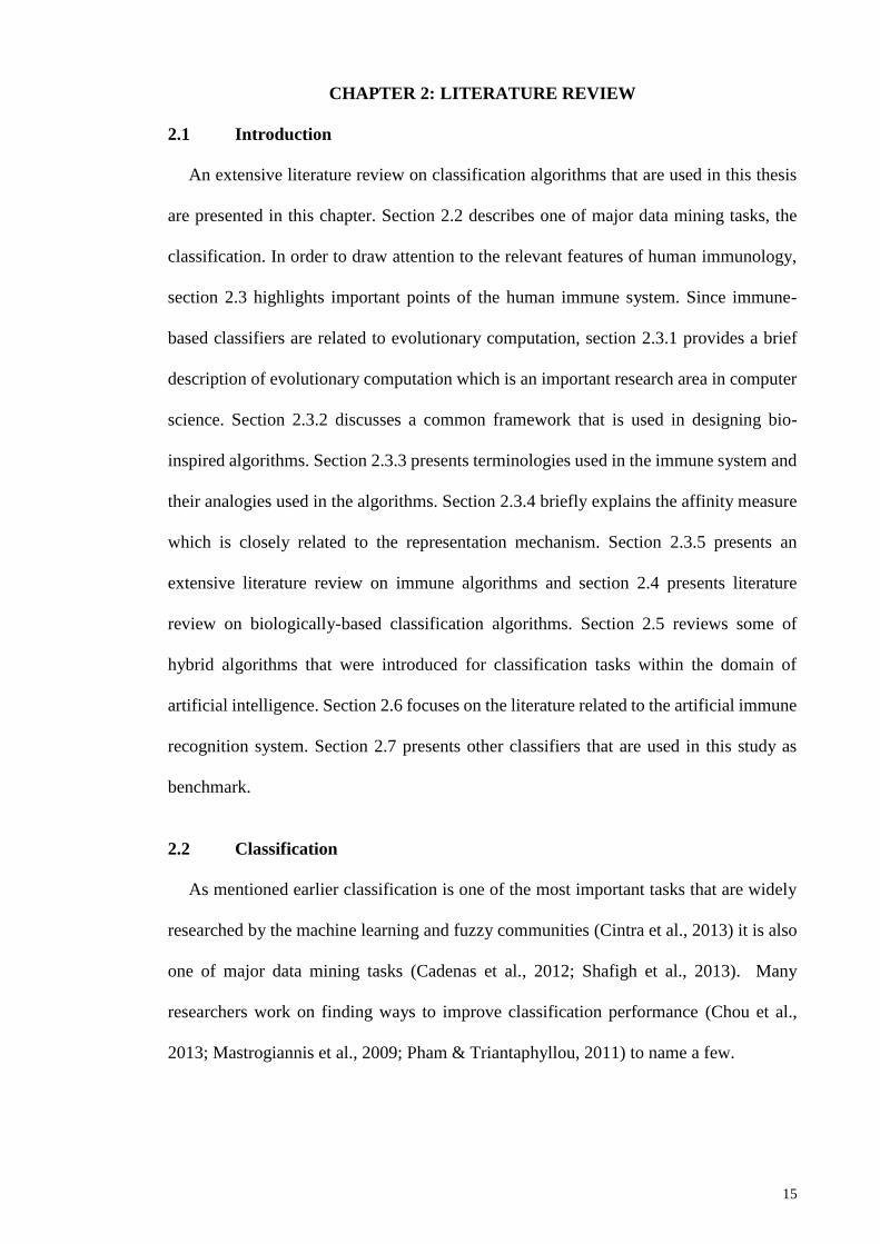
Figure 2.4: Layered Framework for AIS (De Castro & Timmis, 2003) ......................... 30
Figure 2.5: Categories of Artificial Immune System ..................................................... 33
Figure 2.6: Artificial Immune System Taxonomy .......................................................... 33
Figure 2.7: Major Groups of Computational Intelligence ............................................... 37
Figure 2.8: Major Derivatives of Artificial Immune System .......................................... 38
Figure 2.9: Outline of AIRS2 (Watkins, 2005) ............................................................... 47
Figure 2.10: Memory Cell Identification ........................................................................ 48
Figure 2.11: Identifing MCmatch .................................................................................. 49
Figure 2.12: Process of Generating ARBs ...................................................................... 49
Figure 2.13: Clone and Mutate of the Best Match Cell: The MCmatch ......................... 50
Figure 2.14: Process of Resource Allocation and Competition ...................................... 51
Figure 2.15: Flow Chart for Resource Allocation and Competition of AIRS ................ 52
Figure 2.16: Development of MCcandidate and Resource Competition ........................ 55
Figure 2.17: Introduction of Memory Cell to Memory Cell Pool ................................... 55
Figure 3.1: Overview of Research Framework ............................................................... 70
Figure 4.1: Structure and Functional Elements of Fuzzy Control .................................. 89
Figure 4.2: Fuzzy Resource Allocation ........................................................................... 91
Figure 4.3: Resource Allocation for RRC-AIRS2 and FSR-AIRS2 ............................... 92
Figure 4.4: Determine Fuzzy Value for Stimulation ....................................................... 93

xiii
Figure 4.5: Fuzzy Control Language for Resource Allocation of FRA-AIRS2 and
FSRAIRS2 ...................................................................................................................... 95
Figure 4.6: Membership Function for Stimulation ......................................................... 96
Figure 4.7: Membership Function for Fuzzy Stimulation ............................................... 96
Figure 4.8: Pseudocode for RWTS-Resource Competition (RRC) ................................ 99
Figure 4.9: RRC One Level .......................................................................................... 101
Figure 4.10: RRC Two Levels ...................................................................................... 102
Figure 4.11: Pseudocode for RRC-AIRS2 .................................................................... 103
Figure 4.12: Pseudocode for FSR-AIRS2 ..................................................................... 107
Figure 4.13: Comparison of Classification Accuracy AIRS2 versus FRA-AIRS2 on
benchmark data sets ...................................................................................................... 117
Figure 4.14: Comparison of Classification Accuracy AIRS2 versus RRC-AIRS2 on
benchmark data sets ...................................................................................................... 124
Figure 4.15: Comparison of Classification Accuracy AIRS2 versus FSR-AIRS2 on
benchmark data sets. ..................................................................................................... 131
Figure 4.16: Comparison of Balance Scale Accuracy Results ...................................... 132
Figure 4.17: Comparison of Breast Cancer Wisconsin (Diagnostic) Accuracy Results
....................................................................................................................................... 134
Figure 4.18: Comparison of Contact Lenses Accuracy Results .................................... 135
Figure 4.19: Comparison of Ionosphere Accuracy Results .......................................... 136
Figure 4.20: Comparison of Iris Accuracy Results ....................................................... 137
Figure 4.21: Comparison of Liver Disorders Accuracy Results ................................... 138
Figure 4.22: Comparison of Lung Cancer Accuracy Results ....................................... 140
Figure 4.23: Comparison of Pima Indians Accuracy Results ....................................... 141
Figure 4.24: Comparison of Statlog (Heart) Accuracy Results .................................... 142
Figure 4.25: Comparison of Statlog (Image Segmentation) Accuracy Results ............ 143
Figure 4.26: Comparison of Statlog (Vehicle Silhouettes) Accuracy Results .............. 144

xiv
Figure 4.27: Comparison of Sonar, Mines vs. Rocks Accuracy Results ...................... 146
Figure 4.28: Comparison of Vertebral Column_2C Accuracy Results......................... 147
Figure 4.29: Comparison of Vertebral Column_3C Accuracy Results......................... 148
Figure 4.30: Comparison of Wisconsin Breast Cancer Data Set (WBCD) (Original)
Accuracy Results ........................................................................................................... 149
Figure 4.31: Evolved Memory Cells Applying AIRS2 and FRA-AIRS2 ..................... 156
Figure 4.32: Comparison of Data Reduction between AIRS2 and FSR-AIRS2 .......... 157
Figure 4.33: Comparison of Balance Scale Running time Results ............................... 160
Figure 4.34: Comparison of Breast Cancer Wisconsin (Diagnostic) Running time Results
....................................................................................................................................... 162
Figure 4.35: Comparison of Contact Lenses Running time Results ............................. 163
Figure 4.36: Comparison of Ionosphere Running time Results .................................... 164
Figure 4.37: Comparison of Iris Running time Results ................................................ 165
Figure 4.38: Comparison of Liver Disorders Running time Results ............................ 166
Figure 4.39: Comparison of Lung Cancer Running time Results ................................. 167
Figure 4.40: Comparison of Pima Indians Running time Results ................................. 168
Figure 4.41: Comparison of Statlog (Heart) Running time Results .............................. 169
Figure 4.42: Comparison of Statlog (Image Segmentation) Running time Results ...... 170
Figure 4.43: Comparison of Statlog (Vehicle Silhouettes) Running time Results ....... 171
Figure 4.44: Comparison of Sonar, Mines vs. Rocks Running time Results ................ 173
Figure 4.45: Comparison of Vertebral Column_2C Running time Results .................. 174
Figure 4.46: Comparison of Vertebral Column_3C Running time Results .................. 175
Figure 4.47: Comparison of Wisconsin Breast Cancer Data Set (WBCD) (Original)
Running time Results .................................................................................................... 176
Figure 4.48: Comparison of FSR-AIRS2 and Other Classifiers' Area under ROC on
Balance Scale Data Sets ................................................................................................ 178

xv
Figure 4.49: Comparison of FSR-AIRS2 and Other Classifiers' Area under ROC on
Breast Cancer Wisconsin (Diagnostic) Data Set ........................................................... 179
Figure 4.50: Comparison of FSR-AIRS2 and Other Classifiers' Area under ROC on
Contact Lenses Data Set................................................................................................ 181
Figure 4.51: Comparison of FSR-AIRS2 and Other Classifiers' Area under ROC on
Ionosphere Data Set ...................................................................................................... 182
Figure 4.52: Comparison of FSR-AIRS2 and Other Classifiers' Area under ROC on Iris
Data Set ......................................................................................................................... 183
Figure 4.53: Comparison of FSR-AIRS2 and Other Classifiers' Area under ROC on Liver
Disorders Data Set......................................................................................................... 185
Figure 4.54: Comparison of FSR-AIRS2 and Other Classifiers' Area under ROC on Lung
Cancer Data Set ............................................................................................................. 186
Figure 4.55: Comparison of FSR-AIRS2 and Other Classifiers' Area under ROC on Pima
Indians Data Set ............................................................................................................ 187
Figure 4.56: Comparison of FSR-AIRS2 and Other Classifiers' Area under ROC on
Statlog (Heart) Data Set ................................................................................................ 189
Figure 4.57: Comparison of FSR-AIRS2 and Other Classifiers' Area under ROC on
Statlog (Image Segmentation) Data Set ........................................................................ 190
Figure 4.58: Comparison of FSR-AIRS2 and Other Classifiers' Area under ROC on
Statlog (Vehicle Silhouettes) Data Set .......................................................................... 191
Figure 4.59: Comparison of FSR-AIRS2 and Other Classifiers' Area under ROC on
Sonar, Mines vs. Rocks Data Set .................................................................................. 193
Figure 4.60: Comparison of FSR-AIRS2 and Other Classifiers' Area under ROC on
Vertebral Column_2C Data Set .................................................................................... 194
Figure 4.61: Comparison of FSR-AIRS2 and Other Classifiers' Area under ROC on
Vertebral Column_3C Data Set .................................................................................... 195
Figure 4.62: Comparison of FSR-AIRS2 and Other Classifiers' Area under ROC on
Wisconsin Breast Cancer Data Set (WBCD) (Original) ............................................... 197

xvi
LIST OF TABLES
Table 2.1: Mapping between the Immune System and AIRS (Watkins & Timmis, 2002)
......................................................................................................................................... 44
Table 3.1: Data Sets Used in Experiments ...................................................................... 71
Table 4.1: Definitions of Language Elements for Fuzzy Logic ...................................... 88
Table 4.2: Parameter Settings used for AIRS2, FRA-AIRS2, and RRC-AIRS2. ......... 109
Table 4.3: Parameter Settings used for FSR-AIRS2 ..................................................... 111
Table 4.4: Comparative Average Accuracies FRA-AIRS2 versus AIRS2 ................... 113
Table 4.5: Comparing Running Time of AIRS2 versus FRA-AIRS2 .......................... 118
Table 4.6: Comparative Average Accuracies AIRS2 versus RRC-AIRS2 ................... 119
Table 4.7: Comparing Running Time of AIRS2 versus RRC-AIRS2 .......................... 125
Table 4.8: Comparative Average Accuracies................................................................ 127
Table 4.9: Comparison of Classification Results of FSR-AIRS2 and Benchmark
Classifiers on Balance Scale Data Set ........................................................................... 132
Table 4.10: Comparison of Classification Results of FSR-AIRS2 and Benchmark
Classifiers on Breast Cancer Wisconsin (Diagnostic) Data Set .................................... 133
Table 4.11: Comparison of Classification Results of FSR-AIRS2 and Benchmark
Classifiers on Contact Lenses Data Set ......................................................................... 134
Table 4.12: Comparison of Classification Results of FSR-AIRS2 and Benchmark
Classifiers on Ionosphere Data Set ............................................................................... 135
Table 4.13: Comparison of Classification Results of FSR-AIRS2 and Benchmark
Classifiers on Iris Data Set ............................................................................................ 137
Table 4.14: Comparison of Classification Results of FSR-AIRS2 and Benchmark
Classifiers on Liver Disorders Data Set ........................................................................ 138
Table 4.15: Comparison of Classification Results of FSR-AIRS2 and Benchmark
Classifiers on Lung Cancer Data Set ............................................................................ 139
Table 4.16: Comparison of Classification Results of FSR-AIRS2 and Benchmark
Classifiers on Pima Indians Data Set ............................................................................ 140

xvii
Table 4.17: Comparison of Classification Results of FSR-AIRS2 and Benchmark
Classifiers on Statlog (Heart) Data Set ......................................................................... 141
Table 4.18: Comparison of Classification Results of FSR-AIRS2 and Benchmark
Classifiers on Statlog (Image Segmentation) Data Set ................................................. 143
Table 4.19: Comparison of Classification Results of FSR-AIRS2 and Benchmark
Classifiers on Statlog (Vehicle Silhouettes) Data Set ................................................... 144
Table 4.20: Comparison of Classification Results of FSR-AIRS2 and Benchmark
Classifiers on Sonar, Mines vs. Rocks Data Set ........................................................... 145
Table 4.21: Comparison of Classification Results of FSR-AIRS2 and Benchmark
Classifiers on Vertebral Column_2C Data Set ............................................................. 146
Table 4.22: Comparison of Classification Results of FSR-AIRS2 and Benchmark
Classifiers on Vertebral Column_3C Data Set ............................................................. 147
Table 4.23: Comparison of Classification Results of FSR-AIRS2 and Benchmark
Classifiers on Wisconsin Breast Cancer Data set (WBCD) (Original) Data Set .......... 149
Table 4.24: Comparison of Memory Cells Evolved with AIRS2 and FRA-AIRS2 ..... 151
Table 4.25: Comparison of Data Reduction Capabilities of FSR-AIRS2 and AIRS2 .. 158
Table 4.26: Running time measured in seconds [s] on Balance Scale Data Set ........... 160
Table 4.27: Running time measured in seconds [s] on Breast Cancer Wisconsin
(Diagnostic) Data Set .................................................................................................... 161
Table 4.28: Running time measured in seconds [s] on Contact Lenses Data Set ......... 162
Table 4.29: Running time measured in seconds [s] on Ionosphere Data Set ................ 163
Table 4.30: Running time measured in seconds [s] on Iris Data Set ............................ 164
Table 4.31: Running time measured in seconds [s] on Liver Disorders Data Set ........ 165
Table 4.32: Running time measured in seconds [s] on Lung Cancer Data Set ............. 166
Table 4.33: Running time measured in seconds [s] on Pima Indians Data Set ............. 167
Table 4.34: Running time measured in seconds [s] on Statlog (Heart) Data Set .......... 168
Table 4.35: Running time measured in seconds [s] on Statlog (Image Segmentation) Data
Set .................................................................................................................................. 170

xviii
Table 4.36: Running time measured in seconds [s] on Statlog (Vehicle Silhouettes) Data
Set .................................................................................................................................. 171
Table 4.37: Running time measured in seconds [s] on Sonar, Mines vs. Rocks Data Set
....................................................................................................................................... 172
Table 4.38: Running time measured in seconds [s] on Vertebral Column_2C Data Set
....................................................................................................................................... 173
Table 4.39: Running time measured in seconds [s] on Vertebral Column_3C Data Set
....................................................................................................................................... 175
Table 4.40: Running time measured in seconds [s] on Wisconsin Breast Cancer Data Set
(WBCD) Original .......................................................................................................... 176
Table 4.41: Comparison of FSR-AIRS2 and Other Classifiers' Area under ROC on
Balance Scale Data Set.................................................................................................. 178
Table 4.42: Comparison of FSR-AIRS2 and Other Classifiers' Area under ROC on Breast
Cancer Wisconsin (Diagnostic) Data Set ...................................................................... 179
Table 4.43: Comparison of FSR-AIRS2 and Other Classifiers' Area under ROC on
Contact Lenses Data Set................................................................................................ 180
Table 4.44: Comparison of FSR-AIRS2 and Other Classifiers' Area under ROC on
Ionosphere Data Set ...................................................................................................... 181
Table 4.45: Comparison of FSR-AIRS2 and Other Classifiers' Area under ROC on Iris
Data Set ......................................................................................................................... 183
Table 4.46: Comparison of FSR-AIRS2 and Other Classifiers' Area under ROC on Liver
Disorders Data Set......................................................................................................... 184
Table 4.47: Comparison of FSR-AIRS2 and Other Classifiers' Area under ROC on Lung
Cancer Data Set ............................................................................................................. 185
Table 4.48: Comparison of FSR-AIRS2 and Other Classifiers' Area under ROC on Pima
Indians Data Set ............................................................................................................ 187
Table 4.49: Comparison of FSR-AIRS2 and Other Classifiers' Area under ROC on Statlog
(Heart) Data Set............................................................................................................. 188
Table 4.50: Comparison of FSR-AIRS2 and Other Classifiers' Area under ROC on Statlog
(Image Segmentation) Data Set .................................................................................... 189
Table 4.51: Comparison of FSR-AIRS2 and Other Classifiers' Area under ROC on Statlog
(Vehicle Silhouettes) Data Set ...................................................................................... 191
xix
Table 4.52: Comparison of FSR-AIRS2 and Other Classifiers' Area under ROC on Sonar,
Mines vs. Rocks Data Set ............................................................................................. 192
Table 4.53: Comparison of FSR-AIRS2 and Other Classifiers' Area under ROC on
Vertebral Column_2C Data Set .................................................................................... 193
Table 4.54: Comparison of FSR-AIRS2 and Other Classifiers' Area under ROC on
Vertebral Column_3C Data Set .................................................................................... 195
Table 4.55: Comparison of FSR-AIRS2 and Other Classifiers' Area under ROC on
Wisconsin Breast Cancer Data Set (WBCD) (Original) ............................................... 196
Table 4.56: Evaluation of Classifiers on Area under ROC ........................................... 198
xx
LIST OF SYMBOLS AND ABBREVIATIONS
AIRS : Artificial Immune Recognition System
AIS : Artificial Immune Systems
AINE : Artificial Immune NEtwork
ANN : Artificial Neural Network
ARB : Artificial Recognition Ball
AUC : Area Under the ROC Curve
CI : Computational Intelligence
CSA : Clonal Selection Algorithm
DNA : Deoxyribo Nucleic Acid
FIS : Fuzzy Inference System
FRA : Fuzzy-based Resource Allocation
GA : Genetic Algorithm
INT : Immune Network Theory
IS : Immune System
KNN : k Nearest Neighbor
LVQ : Learning Vector Quantization
MLP : Multi-Layer Perceptron
NAT : Network Affinity Threshold
RLAIS : Resource Limited Artificial Immune System
ROC : Receiver Operating Characteristics
RRC : RWTS Resource Competition
RWTS : Real World Tournament Selection
SVM : Support Vector Machine
WEKA : Waikato Environment for Knowledge Analysis

1
CHAPTER 1: INTRODUCTION
1.1 Background and Motivation
Modern computer technologies, sensors and networks have enabled companies,
governments, organizations and all branches of science and engineering to store and
organize massive quantities of data in their databases. The abundant amount of captured
data and generating numerous sets of data in digital form needs to be transformed into
useful knowledge. Increasing the amount of data in science and business has called for
computer-based methods of automatic data analysis where analyst use more sophisticated
and complex tools (Han, Kamber, & Pei, 2012; Kantardzic, 2011).
However, the gap between the storing of data and our understanding is growing and
there is an inverse relationship between them; the greater the increase in volume of data,
the smaller the proportion of it that human understands (Witten, Frank, & Hall, 2011).
The idea that patterns in data can be searched automatically, identified, validated, and
used for prediction has existed among statisticians, economists, communication
engineers, and forecasters for a long time (Witten et al., 2011). However, the
opportunities for discovering patterns in data are increasing at a staggering rate (Witten
et al., 2011).
With the increase in size and complexity of data, it has been inevitable to move away
from the manual data analysis toward automatic data analysis where the analysts use
complex and sophisticated tools (Kantardzic, 2011). Data mining has become the only
hope for finding patterns in a complex world that is overwhelmed by the data. Intelligently
analyzed data is a valuable resource that can lead to new insights (Witten et al., 2011).
There are different definitions for knowledge discovery and data mining, a simple
definition for data mining is: extracting knowledge from large amount of data (Han et al.,
2012) and a more comprehensive definition is: a nontrivial procedure of detecting valid,

2
previously unknown, potentially useful patterns in observed data, and ultimately
communicating the discovered knowledge to people in an understandable way (Feyyad,
1996; Goebel & Gruenwald, 1999). The whole procedure of applying computer-based
techniques for retrieving knowledge from data is basically called data mining
(Kantardzic, 2011). Data mining has been heavily used by insurance companies, banks,
credit card issuers, manufacturing firms, telephone companies, drug and food industries,
in the medical field, police and security agencies, and many other applications. Data
mining is among the most rapidly growing field in the computer science (Kantardzic,
2011). Thus, data mining is a technique for discovering previously unknown, hidden and
useful information that would assist users in making proper decision.
There are several approaches to illustrate hidden patterns including classification,
clustering, sequential pattern discovery, and association rule discovery (Soman, Diwakar,
& Ajay, 2006).
One of the most commonly used tasks in data mining is classification (Džeroski, 2010).
It is about classifying instances into two or more pre-determined classes. Classification
rules are extracted from a set of pre-classified instances, this set is called training set and
the actual procedure of extracting the classification rules is known as learning.
The tasks of classification and pattern recognition are common to many scientific,
medical and engineering applications. Common subjects among researchers in the field
of science, medicine and engineering are classification and pattern recognition. In recent
years, the data mining area has attracted scientists in numerous fields including machine
learning and many classifiers have been widely studied and have served as solutions for
the classification and machine learning problems. Classification is one of the most
important tasks that are widely researched by the machine learning and fuzzy
communities (Cintra, Monard, & Camargo, 2013). Classification is also known as one of

3
major tasks of data mining (Cadenas, Garrido, Martínez, & Bonissone, 2012; Shafigh,
Hadi, & Sohrab, 2013). Maximizing the predictive accuracy of a classifier is one of the
most important goals of classification algorithm (Pappa & Freitas, 2010). Improving
classification performance is very important and many researchers across the globe work
on finding ways to achieve this goal (Chou, Cheng, & Wu, 2013; Mastrogiannis,
Boutsinas, & Giannikos, 2009; Pham & Triantaphyllou, 2011) to name a few. Still, many
of the presently existing classifiers are computationally intensive, which makes them
sometimes unsuitable to be applied on real-life issues that require immediate response.
Furthermore, many of them are not intuitive in mimicking the learning behavior of human
being (Witten et al., 2011).
Data mining employs machine learning methods, mathematical algorithms and
statistical models to discover valid relationships and patterns in large data sets (Dua &
Du, 2011).
Machine learning consists of computational methods that are applied to data in order
to discover or learn new things about the data, or to be able to predict an outcome, based
on some prior knowledge (Timmis & Knight, 2002). Machine Learning: is a subfield of
AI, which is concerned with programs that learn from experience (Russell & Norvig,
2016). Programs use sample data or experience for optimizing a performance criterion.
Being a part of AI, machine learning needs to be intelligent; because in a changing
environment, the program should have the ability to learn. Program designer does not
need to predict and offer solutions for all possible circumstances. Machine learning
applies statistical theories to build mathematical models, since its major task is to infer
from samples (Alpaydin, 2014).

4
From the information-processing perspective it is remarkable that the immune system
(IS) is a highly adaptive, distributed and parallel system, it is based on principles of the
natural system, which is capable of solving complex classification tasks. It learns to
recognize relevant patterns, remember previously identified patterns, and builds pattern
detectors efficiently, it is also capable of feature extraction, self-regulation and fault
tolerance, these tasks are very important in the field of natural computation (Dipankar
Dasgupta, 1999; De Castro & Timmis, 2002b). The human immune system is capable of
undertaking a myriad of tasks it can cope with highly dynamically changing situations,
while it maintains a memory of past events, it is capable of continually learning about
new events (Dipankar Dasgupta, 1998; Timmis & Knight, 2002). The immune system
has offered productive ideas for models of computation and from the computational point
of view, the most important features are the capabilities to generalize, remember, and
classify confronted substances (Watkins, 2001).
These abilities have inspired scientists and researchers to build systems that are able
to mimic various computationally appealing features of the immune systems (Timmis,
Knight, De Castro, & Hart, 2004), they are able to solve a variety of computationally
based problems. One of these systems is called Artificial Immune Systems (AIS). The
AIS is an immune system inspired computational system that is also categorized under
computational intelligence (Brownlee, 2011; Elsayed, Rajasekaran, & Ammar, 2012).
AIS is also known as one of the artificial intelligence techniques that offers robust and
strong information processing capabilities for solving problems (Leung, Cheong, &
Cheong, 2007a). AIS, is actually a class of adaptive algorithm (Brownlee, 2005) that
abstracts the structure and function of the human immune system into computational
systems (Wikipedia, 2012). The field of AIS has attracted many researchers, and has
found a wide range of theoretical discussions and application domains. Applications of
AIS are increasing rapidly and AISs are offering robust and powerful information

5
processing capabilities for solving complex problems (Leung et al., 2007a). They are also
building progressively an effective division of computational intelligence within data
mining and knowledge discovery field.
Artificial Intelligence (AI): The term AI is applied when a machine imitates cognitive
functions that humans associate with other human minds, such as learning and problem
solving. The definition for AI is still incomplete; however, researchers have identified
four possible goals to follow in AI: one of the goals is concerned about thought processes
and reasoning, another one is about behavior, another one is about measuring success in
terms of human performance, and the last one is about rationality, which measures against
an ideal concept of intelligence. AI has been grouped in four categories: Systems that
think like humans, systems that think rationally, systems that act like human, and systems
that act rationally (Russell & Norvig, 2016).
Scientists, mathematicians, engineers, and other researchers have been interested in
the capabilities of AIS, and AIS has found applications in a wide variety of areas, some
of them are: anomaly detection (Dipankar Dasgupta & Forrest, 1998; Greensmith,
Aickelin, & Tedesco, 2010; Yi, Wu, & Chen, 2011); classification (Carter, 2000; Leung,
Cheong, & Cheong, 2007b; Watkins, Timmis, & Boggess, 2004; Zhang & Yi, 2010);
clustering (Graaff & Engelbrecht, 2011; Knight & Timmis, 2003; Tang & Vemuri, 2005);
data analysis (Drozda, Schaust, Schildt, & Szczerbicka, 2011; Timmis, 2000; Timmis,
Neal, & Hunt, 2000); machine learning (Cheng, Lin, Hsiao, & Tseng, 2010; Das &
Sengur, 2010; De Castro & Von Zuben, 2002; Glickman, Balthrop, & Forrest, 2005;
Knight & Timmis, 2003); pattern matching, recognition (Dipankar Dasgupta, Yu, &
Majumdar, 2003; Tarakanov & Skormin, 2002); web data mining (Mao, Lee, & Yeh,
2011; Nasaroui, Gonzalez, & Dasgupta, 2002; Rahmani & Helmi, 2008; Yang, Kiang,
Chen, & Li, 2012; H. Zhao, Chen, Zeng, Shi, & Qin, 2011).

6
AIS is a computational paradigm in artificial intelligence and its focus was mainly on
the development of unsupervised learning algorithms rather than the supervised one
(Watkins & Timmis, 2002). AIS was designed and developed for data clustering or
feature extraction, therefore its performance for classification was not satisfactory.
Watkins and Timmis (Watkins, 2001) introduced Artificial Immune Recognition System
(AIRS) which was designed to fill the gap and focus on classification problems
(Brownlee, 2005).
The interest for immune-system-inspired information processing algorithms such as
AIRS have been growing (Chikh, Saidi, & Settouti, 2012; Tay, Poh, & Kitney, 2013).
More recently there have been substantial efforts in exploiting and exploring the potential
of AIRS for applications in computer science, medicine and engineering. AIRS was
designed specifically and applied to classification problems. As discussed earlier,
scientists were motivated by several characteristics of the immune systems of mammals,
such as learning and recognition capabilities and they have been developing algorithms
for a broad spectrum of applications. Some of these algorithms are concerned with
classification issues; these are very common real-world data mining tasks. AIRS is a
competitive classification system (Brownlee, 2005), and it is comparable to well-
established classifiers in terms of accuracy (Golzari, 2011; Tay et al., 2013).
AIRS is a reasonably complex algorithm which has demonstrated substantial
accomplishments on a broad range of classification problems (Brownlee, 2005), and it is
well-known that classification problems play a significant role in data mining and
computer science (Shafigh et al., 2013; Zhu & Guan, 2004). AIRS has enhanced
considerably the classification performance (Polat, Şahan, Kodaz, & Güneş, 2007), and
it has been identified as an effective classifier for a number of machine learning problems

7
(Doraisamy & Golzari, 2010; Goodman, Boggess, & Watkins, 2003). A recent study
argues that the methodology of AIRS is useful for data classification (Tay et al., 2013).
Even though AIRS has shown many good features, it has the potential to accomplish
even better. Given the excellent results, AIRS has rooms for improvement and is deserved
to be investigated (Brownlee, 2005), and its full potential is still unleashed (Tay et al.,
2013). A recent study carried out by (Jenhani & Elouedi, 2012) demonstrated that
insufficient efforts have been made for improving the classification accuracy of AIRS,
they argued that the bulk of circulated articles is about applications of AIRS for solving
“real-world” problems; however few works were dedicated to improving the algorithm
itself. In particular they argued that the use of k nearest neighbor may reduce the accuracy
of AIRS (Jenhani & Elouedi, 2012). Polat et al. have demonstrated that classification
performance of AIRS could be improved if the number of resources and running time
were reduced (Polat, Şahan, Kodaz, et al., 2007). Golzari et al. have documented that one
of the problems of the AIRS is its very high selection pressure during resource
competition; they argued that this causes loss of diversity, and may produce premature
memory cells. They argued that high selection pressure decreases the classification
accuracy (Golzari, Doraisamy, Sulaiman, & Udzir, 2009a). On the other hand, AIRS’
classifier is the k-Nearest Neighbor (KNN), and it is known in the machine learning that
KNN does not demand for an exact match with any cases or stored patterns, in order to
identify patterns of data which means, arguably, low accuracy. In addition choosing k for
KNN may affect the performance of KNN, if k is chosen to be too small, the outcome
might be subtle to noise in data, and if k is chosen to be too large, then it is possible to
have points from other classes in the neighborhood (Wu et al., 2008).
One of common practice for improving classification accuracy is using hybrid models
through combining several models together; the goal of the hybrid models is using unique

8
capability of each component in order to improve pattern recognition in the data
(Khashei, Zeinal Hamadani, & Bijari, 2012). It is also known that AISs are hybrid systems
(De Castro & Timmis, 2002b) and literature review reveals that concepts of AIS have
been used in connection with classifiers such as KNN and SVM for different purposes
and applications. For example a hybrid of AIS and KNN was used for pattern recognition
by (W. Zhao & Davis, 2011) and Şahan et al. introduced a hybrid of fuzzy AIS and KNN
algorithm to classify breast cancer data set (Şahan, Polat, Kodaz, & Güneş, 2007). Hybrid
of AIS and SVM were also developed by researchers, a recent approach shows the use of
AIS-SVM algorithm for anomaly detection by (Aydin, Karakose, & Akin, 2011) and in
another research study, a hybrid of AIS-SVM ensemble has been successfully used for
text classification (Antunes, Silva, Ribeiro, & Correia, 2011b). Researchers also
developed AIS-SVM hybrid algorithm to identify voltage collapse prone areas and
overloaded lines in the power system (Woolley & Milanović, 2009).
AIRS is considered as a hybrid of elements and methods developed for supervised and
unsupervised artificial immune system’s algorithms (Brownlee, 2005). Watkins applied
KNN inside AIRS in order to carry out the classification tasks. KNN have been added to
other components and procedures to create what is known as AIRS thus, it could also be
interpreted as a hybrid algorithm of AIRS that includes KNN. Some researchers even
argued that AIRS is a pre-processor for KNN (Seeker & Freitas, 2007) Although this
remark is correct, however a review of the literature clearly reveals that AIRS has been
accepted as a classifier by all other researchers on the topic of AIRS.
A hybrid algorithm is a composite of two or more algorithms that are created in order
to perform tasks in a new and eventually more sophisticated fashion. As such, AIRS is a
hybrid algorithm, which has borrowed concepts from various algorithms in the field of
artificial intelligence such as: AIS (Brownlee, 2005), Artificial Recognition Ball (ARB)

9
(Farmer, Packard, & Perelson, 1986), Artificial Immune NEtwork (AINE) (Thomas
Knight & JonathanI Timmis, 2001; Watkins, 2005) and random mutation, clonal
expansion, and clonal selection from other AIS-based algorithms (Brownlee, 2005).
Because of the need for new and efficient ways of classification, researchers have been
developing hybrid algorithms with the aim of improving classification accuracy,
performance of classifiers and obviously for solving specific problems. Literature review
reveals that there exists no hybrid model of AIRS-SVM algorithm, both AIRS and SVM
have strengths that when combined could lead to a new and more efficient immune based
classifier.
Classifiers play an important role in solving real-world problems, and AIRS, as an
immune inspired classifier needs further improvement. As a contribution to the field of
computer science and artificial intelligence, this study introduces a modification of AIRS
which enhances the classification accuracy and retains or improves performance and
efficiency of the resulting classifier.
1.2 Research Problem
AIRS is an effective and well-known classifier (Igawa & Ohashi, 2009). AIRS'
performance is higher than other classifiers (Deng, Tan, He, & Ye, 2014) or comparable
to well-respected classifiers in terms of accuracy (Golzari, 2011; Tay et al., 2013) and it
has the following desirable algorithmic characteristics: it is self-regulatory, efficient,
stable under a wide range of user-set parameters, and has data reduction capability. There
is no need for the user of the AIRS to select any architecture during training phase since
its adaptive process discovers an appropriate architecture automatically. AIRS does not
use the whole training dataset for classification, instead the algorithm uses a minimum
number of exemplars to create new training instances and then produces the resulting
classifier (Brownlee, 2005). One study evaluated AIRS as a stable classifier with near
10
average results and concluded it can safely be added to the data mining toolbox (Meng,
van der Putten, & Wang, 2005; Van der Putten, 2010). In fact, AIRS is listed (Machaka,
Mabande, & Bagula, 2012) as one of the classifiers in the data mining tool, the WEKA,
which has been developed at the university of Waikato in New Zealand (Soman et al.,
2006) and maintained by (Mark Hall et al., 2009). The WEKA is considered as a popular
workbench in the domain of machine learning (Bouckaert et al., 2010) and a
comprehensive tool bench for both machine learning and data mining (Soman et al.,
2006).
Although AIRS has shown to have many good features, it still has the potentials to
perform even better. The full potential of the AIRS is still unleashed (Tay et al., 2013).
Researchers have identified some weaknesses that needed to be addressed. Jenhani &
Eloudi showed that relatively few efforts have been made to improve the classification
accuracy of AIRS, majority of published articles have applied AIRS to solve a particular
classification problem (Jenhani & Elouedi, 2012). Intensive research on AIRS shows that
following problems needed to be addressed:
As mentioned earlier, AIRS is a hybrid algorithm that uses the concepts of AIS
and KNN to perform classification tasks. AIRS uses k-NN as a classifier, and in
machine learning, KNN was developed in such a way that it identifies patterns of
data without demanding for an exact match to any cases or stored patterns, this
means, relatively speaking, low accuracy. Also selecting k for KNN affects the
performance of KNN, if k is chosen to be too small, the result might be sensitive
to noise in data, and if too large a value of k is, then the neighborhood may include
points from other classes (Wu et al., 2008) and KNN also tends to be
computationally expensive (Goodman, Boggess, & Watkins, 2002). SVM and
KNN are among the top 10 classifiers (Wu et al., 2008) however, without looking

11
at the application of KNN in AIRS, outcome of other researches have revealed
that SVM outperforms KNN (D. S. Huang, Gan, Bevilacqua, & Figueroa, 2011)
this is particularly true when the number of features increases (Hmeidi, Hawashin,
& El-Qawasmeh, 2008). A recent research has also indicated that using KNN
reduces the classification accuracy of AIRS (Jenhani & Elouedi, 2012). Despite
the superiority of SVM over the KNN, to the best knowledge of this research,
there exist no hybrid algorithm that uses the concepts of the AIRS and the SVM.
Therefore this research aims to verify whether or not a hybrid algorithm dubbed
as FSR-AIRS2 (see section 4.4) which uses SVM as the classifier will perform
better than AIRS2.
AIRS has inherited many of the elements from the Artificial Immune Network
(AINE), which is a form of clonal selection algorithm, such as the concept of the
Antigen Recognition Ball (ARB) (see details in section 2.4), and an unusual way
of resource limitation for controlling the population size; an ARB presents the
idea of cell concentrations into clonal selection, and represent a data structure of
multiple, identical antibodies, therefore, a population of ARBs represents a much
bigger population of antibodies more efficiently (Garrett, 2005). Intensive
comparison of the AIRS with the Learning Vector Quantization (LVQ) method,
introduced by (Kohonen, 1990), have shown mixed results (Goodman et al., 2002;
Watkins & Timmis, 2002) Garrett argued that AIRS outperforms LVQ, however
it tends to do so by using high computing resources (Garrett, 2005; Golzari, 2011;
Golzari, Doraisamy, Sulaiman, Udzir, & Norowi, 2008; Polat & Güneş, 2007),
and the use of a linear method for allocating resources, causes high running time
(Golzari, Doraisamy, Sulaiman, & Udzir, 2011).
Generally a high selection pressure causes premature convergence (Ahn, 2006).
Although high selection pressure can increase the speed of optimization, it

12
increases the probability of getting stuck in local optima. It means we have a trade-
off between accuracy and efficiency (Kramer, 2008). Golzari et al. have identified
that AIRS' selection pressure is very high during resource competition, and this
leads to loss of diversity, and may cause premature memory cells. If selection
pressure becomes too weak, the population may drift aimlessly for a long time,
and the quality of the solutions found is not likely to be good. On the other hand,
rapid convergence is desirable, but an excessively fast convergence may cause the
algorithm to converge prematurely to a suboptimal solution (Cantú-Paz, 2000).
Thus the consequence of high selection pressure is decreased classification
accuracy (Cantú-Paz, 2000; Golzari, 2011; Golzari, Doraisamy, Sulaiman, &
Udzir, 2009b).
1.3 Research Objective
The main objective of this thesis is to address the shortfalls explained in the previous
subsection and to demonstrate and explore the classification capabilities through a
detailed presentation of the proposed algorithms and through an evaluation of the
algorithm’s performance on real world datasets that have been used throughout machine
learning literature. The datasets are introduced in subsection 3.3.2. This objective is
achievable by undergoing the following processes:
Introducing a new resource allocation method based on fuzzy logic in order to
reduce number of resources and increase the classification accuracy of AIRS2.
This method is dubbed as Fuzzy-based Resource Allocation (FRA-AIRS2).
Introducing a new resource competition method for AIRS2 based on the concept
of real world tournament selection in order to reduce premature memory cells and
thus increase the classification accuracy. This method is dubbed as Real-world-
tournament-selection-based Resource Competition (RRC-AIRS2).
13
Introducing and evaluating a new immune inspired hybrid system of instance handling
components of AIRS2 and SVM with the goal of improving performance of AIRS2, in
particular, its classification accuracy. The new hybrid model consisting of concepts used
in FRA-AIRS2, RRC-AIRS2, SVM, and AIRS2. The new hybrid model is dubbed as
FSR-AIRS2.
1.4 Research Scope
Given the fact that classification is one of the most important tasks of data mining, and
that there is increasing number of applications of AIRS for real-world data mining tasks,
this thesis focuses on the AIRS algorithm and develops a new algorithm with the goal of
improving AIRS’ performance. For reducing and controlling the number of resources
this study uses fuzzy logic during resource allocation stage of the algorithm; in order to
avoid premature memory cells and reducing loss of diversity, RWTS method is applied
during resource competition stage of the algorithm; and in the classification stage, this
study incorporates SVM as the classifier instead of KNN.
This study uses a wide range of publicly available real world datasets from UCI
machine learning repository.
The following performance measures will be carried out: classification accuracy, n-
fold cross validation, data reduction, overall runtime, area under ROC (AUC), and
student’s t-test. These measures are discussed in detail in section 3.4.
1.5 Thesis Outline
This section describes the structure and content of the thesis. The chapters of this thesis
are organized as described below.
Chapter 2 provides the relevant background on classification tasks and presents an
overview of the human immune system and evolutionary computing. Then it introduces

14
the common framework used for designing bio-inspired computational algorithm. Next
this chapter presents terminologies used in the immune system and their counterparts used
in the algorithms, followed by a brief explanation of affinity measures. Then it presents
an extensive literature review on immune algorithms, biologically-based classification
algorithms, and artificial immune recognition system.
Chapter 3 explores the methodology used in this study. It gives an overview of the
research and presents the experimental setup including system specification, datasets and
parameter setup. Further this chapter provides a brief overview of performance metrics
used in this dissertation.
Chapter 4 presents details of the proposed algorithm, it evaluates the performance of
the new algorithms on benchmark datasets and compares its performances with that of
AIRS2 and some well-known algorithms and discusses the results of experiments.
Chapter 5 provides a summary of the dissertation, its contribution to the field of
computer science and data mining, and outlines the conclusions that can be drawn and
there are some comments on future extensions of this work.
15
CHAPTER 2: LITERATURE REVIEW
2.1 Introduction
An extensive literature review on classification algorithms that are used in this thesis
are presented in this chapter. Section 2.2 describes one of major data mining tasks, the
classification. In order to draw attention to the relevant features of human immunology,
section 2.3 highlights important points of the human immune system. Since immune-
based classifiers are related to evolutionary computation, section 2.3.1 provides a brief
description of evolutionary computation which is an important research area in computer
science. Section 2.3.2 discusses a common framework that is used in designing bio-
inspired algorithms. Section 2.3.3 presents terminologies used in the immune system and
their analogies used in the algorithms. Section 2.3.4 briefly explains the affinity measure
which is closely related to the representation mechanism. Section 2.3.5 presents an
extensive literature review on immune algorithms and section 2.4 presents literature
review on biologically-based classification algorithms. Section 2.5 reviews some of
hybrid algorithms that were introduced for classification tasks within the domain of
artificial intelligence. Section 2.6 focuses on the literature related to the artificial immune
recognition system. Section 2.7 presents other classifiers that are used in this study as
benchmark.
2.2 Classification
As mentioned earlier classification is one of the most important tasks that are widely
researched by the machine learning and fuzzy communities (Cintra et al., 2013) it is also
one of major data mining tasks (Cadenas et al., 2012; Shafigh et al., 2013). Many
researchers work on finding ways to improve classification performance (Chou et al.,
2013; Mastrogiannis et al., 2009; Pham & Triantaphyllou, 2011) to name a few.
16
Classification is a process of assigning an object into a predefined class or group based
on observation of a number of attributes belonging to that object. It is also a process of
finding a set of functions or models that differentiate and describe data concepts or data
classes with the goal of being able to use the model for predicting the class of objects
whose class label is unknown. Many problems in areas such as medicine, loan approval,
business, and industry can be treated as classification applications. Some examples are:
classifying financial marketing trends, bankruptcy prediction, credit scoring, image and
pattern recognition, speech recognition, handwritten character recognition, medical
diagnosis, and quality control (Han et al., 2012).
The major strength of classification is that it is possible to classify data into groups of
known labels; it is quantifiable and may use statistical methods for classification.
However, the weakness is that we need labled data, which are often difficult to obtain,
the effect of labeling may be stigmatisation, and the question of correct labelling may
arise. It is also desirable to have equal proportion of data for each class label.
Classification tasks have specific goals; they use instances with known class labels for
constructing a predictive model in which class labels are assigned to the new instances.
Most classification methods are built in two-stages, which are cleanly separated: the
initial stage or the training phase, where the algorithm uses one part of a dataset to analyze
and learn the underlying classes. A training dataset consists of a number of instances, and
each instance consists of attributes, also known as features. Each training vector can be
represented by T = {(𝑥𝑖,𝑦𝑖) | 𝑥𝑖𝑚 , 𝑦𝑖Ƶ
𝑛 {0, 1, 2, …} , i= 1,2,...,n}, where 𝑥𝑖 is a real
m-dimensional input vector and each 𝑦𝑖 represents the class label to which the point
𝑥𝑖 belongs. In a supervised learning the class label of each instance is known, while in an
unsupervised learning the class label is not known (Han et al., 2012).

17
The second stage of classification is called the training phase, in this stage the model
which was built in the first stage is used for classification. Initially the predictive accuracy
of the classifier has to be estimated, if the accuracy is acceptable, then the classifier can
be used to predict class label of new, previously unknown instances (Han et al., 2012).
Examples for models that use the training data are support vector machines, neural
networks, rule-based methods, and decision trees (Aggarwal, 2014b). Use of test data set
in estimating the accuracy also helps to avoid overfitting. Evaluation is essential for
making real-progress in data mining (Witten et al., 2011) and machine learning, with a wide
range of existing classifiers there is a need to measure their performance. The common
approach to assessing the classifier’s accuracy is to evaluate its error rate on an
independent test set of instances, held back from the training data set (Witten et al., 2011).
Not only there are different kinds of classifiers but also many classifiers come with different
options and parameters that can be set by the users, different settings may lead to different
results (Golzari, 2011). A classifier’s accuracy is the percentage of correctly classified
instances by the classifier, related class label of each test record is then compared with
the class label of the learned classifier for the same instance. Misclassification happens
when a classifier predicts a wrong class for an instance, and the error rate is the ratio of errors
made over entire set of instances (Witten et al., 2011).
It is wishful to have a classifier that makes no error on all data sets mostly because of lack
of adequate information about underlying data sets and possible noise.
The importance of evaluation of a new approach was emphasized by (Adya & Collopy,
1998) in their survey. They emphasized that a new approach must be compared with
alternatives that are or could be used; otherwise, it is difficult to argue about the value of the
model.

18
Some criteria for evaluation of classification performance are: classification accuracy,
n-fold cross validation, data reduction, overall runtime, area under the ROC curve. All
these performance criteria are presented in detail in subsection 3.4.
Different techniques are used in various classification algorithms; some of them are:
support vector machines, rule-based techniques, decision-tree learning algorithm,
instance-based learning algorithms, statistical-based learning algorithm, and biologically-
inspired techniques. The latter one includes techniques that are based on Artificial Neural
Network, Genetic Algorithm, and AIS (Golzari, 2011). Figure 2.1 illustrates some
common classification techniques. The focus of this thesis is mainly on AIS-based
algorithms.
Figure 2.1: Common Classification Techniques
Classification Techniques
Biologically-inspired Techniques
Artificial Immune System (AIS)
Genetic Algorithm (GA)
Artificial Neural Network (ANN)
Support Vector Machines (VM)
Rule-based Techniques
Decision-tree Learning Algorithm
Instance-based Learning Algorithms
Statistical-based Learning Algorithm

19
Improving the performance of AIRS2, and AIS-based algorithm is the focus of this
study. AIRS2 has shown comparable performance with other classifiers and it is identified
as one of the clever algorithms (Brownlee, 2011).
The rest of this section focuses on a brief introduction and description of some
common supervised learning (classification) techniques.
There are two types of learning algorithms: lazy and eager. The difference between
these two types is that while lazy learning algorithm postpones the work as long as
possible, eager methods produce a generalization immediately after the data has been seen
(Witten et al., 2011). In other words lazy method works little during the training and does
more during the classification phase, whereas eager learning algorithm the model tries to
build a generalization function during training of the model (Golzari, 2011; Hendrickx &
Van den Bosch, 2005). Hardarean et al. provided a comparative analysis of the lazy and
eager methods (Hadarean, Bansal, Jovanović, Barrett, & Tinelli, 2014), and showed that
they are complementary in terms of the kind of problems they can solve. In their study of
deciding bit-vector constrains, they argued that in contrast to the eager approach, the lazy
methods provide a wide range of optimization techniques that are only available to the
lazy approach. Their empirical evaluation also showed that lazy solver were able to solve
such problems that the eager solvers failed to solve.
Instance-based classification algorithms belong to the family of the lazy learning
algorithms. In instance-based classification, a distance metric is used to compare each
new instance with the existing ones, and the class of the nearest (closest) existing instance
is used to assign it to the new instance. This is known as the nearest-neighbor
classification algorithm. It may happen that there is more than one nearest-neighbour; in
this case majority vote method is used to determine the class of the new instance, meaning
the majority class of closest k neighbours is assigned to the new instance. This is the well-

20
known k-Nearest Neighbour (KNN) method (Witten et al., 2011). The most popular
distance metrics are the Euclidean and the Manhattan distance (Golzari, 2011; Shahid,
Bertazzon, Knudtson, & Ghali, 2009). Examples for eager learning models are: artificial
neural network, linear regression, and support vector regression (Wei, 2015).
One of popular classification methods is the decision tree; this is because its
construction does not need any domain knowledge or parameter setting which makes it
suitable for exploratory knowledge discovery. Decision tree looks like a flowchart tree,
where each internal node represent a test on an attribute, each branch denotes an outcome
of the test, and each leaf node holds a class label (Han et al., 2012). Quinlan (Quinlan,
1986) argued that because of the simplicity, decision trees are natural ways for decision
makings however, it is more complex to learn decision trees from the data. Decision tree
algorithms have found extensive applications in machine learning and classification tasks
(Gokgoz & Subasi, 2015). Construction of decision trees involves two stages, the first
stage the tree is growing here the algorithm uses attribute selection measures to select the
best feature that discriminate between the distinct classes and then splits the data into two
new nodes based on that feature. This is applied recursively to the resulting data subsets
until a class assignment can be made for each leaf. After decision trees are constructed,
many branches may represent outliers or noise in the training instances, therefore the
second stage known as pruning jumps in, it attempts to identify and clip off branches of
the tree that are least useful in order to improve the classification accuracy on the training
data with the complexity of the model (Han et al., 2012; Nisbet, Elder, & Miner, 2009).
Quinlan got the idea of developing the predecessor of the C4.5, the ID3 (Quinlan, 2014),
from the Hunt’s Concept Learning Systems. C4.5 is one of widely used decision trees, it
was developed by (Quinlan, 1993). C4.5 has been frequently used as a benchmark for
comparing newer supervised learning algorithms (Han et al., 2012). C4.5 applies an
entropy-based information gain measure to find most relevant feature to grow decision

21
tree (T.-h. Kim et al., 2011). It starts with a general tree and continues to grow until
maximum classification is achieved; it then clips off the tree as far as possible up to pre-
set adequate misclassification rates (T.-h. Kim et al., 2011). C4.5 uses the pruning process
to solve the over-fitting problem (Mantas & Abellán, 2014).
One of the oldest and well-known classifier is Bayes classifier (Duda & Hart, 1973) it
is based on Bayesian theorem (Nisbet et al., 2009) with strong independent assumptions.
Document classification is one of good applications of Naïve Bayes classifier (Aggarwal,
2014a). It computes the likelihood that a given instance belongs to a particular class. It
has shown high speed and accuracy when applied to large databases (Han & Kamber,
2006). A simple Bayesian classifier known as Naïve Bayesian classifier is comparable to
decision trees in terms of performance (Han & Kamber, 2006).
Bayes’ classifier would need two parameters to do the classification namely the ‘a
priori probability’ and the ‘class conditional density’; however in practice it is possible
that both parameters are unknown and that makes the classification task difficult.
Therefore Bayes’ classifier tries to estimate the class based on limited conditions
(Bandyopadhyay & Pal, 2007). The probability of the class labels are easily estimated
from the training data, however estimating the distribution of attribute values given the
class is more complex. For this purpose, the Bayes rule is used to calculate the conditional
likelihood of the class given the attributes. After the classifier has been trained, it is used
for classification of new instances. Applying Bayes’ theorem, it is possible to determine
the posterior probability of each class, and then the new instance will get the class with
maximum posterior probability (Bethlehem & Van Der Heijden, 2000). Some researchers
have argued that prior probabilities of Naïve Bayes are unreliable, and have shown that
prior probabilities might yield an incorrect classification (Gelgi, Vadrevu, & Davulcu,
2007).

22
Artificial neural network is a mathematical model that simulates human neural system.
An artificial neural network consists of multi-layers and nodes, where nodes represent the
neurons on human neural system. Connections between the nodes are known as weights,
their values depend on the learning procedure (Kecman, 2001). If a classification problem
consists of m-classes and n-features, the neural network will have m input and n output
nodes. Throughout the learning phase, artificial neural network try to adjust weights in
order to get optimal outputs. Once the learning phase is over, artificial neural network
assigns the class with the maximum output to the new unknown instance (Golzari, 2011).
One drawback of the neural network is that the training process is inefficient and that the
knowledge representation is unknown (Chien, Lin, & Yang, 2006; Golzari, 2011). In
another study, Osyk et al. reported that producing false alarms was the primary weakness of
the neural network (Osyk, Hung, & Madey, 1994).
2.3 From Human Immune System To Artificial Immune System
One of the tasks of the immune system is to attack and try to eradicate pathogens or
other infectious organisms that invade human body (Timmis et al., 2004). The human
immune system consists of a network of cells, tissues, and organs that work together to
protect the body (Prasad, 2010). Leucocytes or white blood cells are engaged in finding
and destroying disease-causing substances or organisms (Prasad, 2010). There exits two
basic types of leukocytes: phagocytes and lymphocytes, in this thesis we focus only on
lymphocytes. The lymphocytes empower the body to remember and recognize previously
identified pathogens (invaders) and help the body to destroy them (Sompayrac, 2012).
There are two types of leukocytes: B-lymphocytes and T-lymphocytes. Lymphocytes
originate from bone marrow where they can mature into B cells or move to thymus gland
and mature into T cells (Sompayrac, 2012). B cells and T cells have different
functionalities, while B cells seeks their targets and use defense mechanism to lock onto
them, T lymphocytes (cells) are responsible for eliminating the invading germs after being

23
identified by the immune system (Sompayrac, 2012). The process of affinity maturation
which is also known as immunological B-cell maturation is a process of variation and
selection, undifferentiated B cell transform to one that secretes antibodies with particular
specificity. These antibodies are specialized proteins that lock only onto specific antigens
(Sompayrac, 2012). This transformation and activation of the B cell occurs when its
affinity threshold is exceeded. While antibodies bind to pathogens and inactivate them,
B-cell clones itself. However, produced clones are not faultless. The cloning process is
vulnerable to very high mutation rates which means cloned B cells may have to some
extent different receptors from their parents. These new cloned cells will also have the
opportunity to bind with the pathogens. To determine which B cell is the strongest, B
cells compete for available pathogens. Some cells will have stronger affinity levels than
others, and B cell with highest affinity for the pathogens is the "fittest" and therefore will
be cloned or replicated the most. Hyper-mutation provides the variation aspect, and the
selection aspect is provided by competition for pathogens (Hofmeyr & Forrest, 2000).
Figure 2.2 shows B cell activation pathway, when a B cell comes across its specific
antigen, with the help of T cells, B cell multiply and mature into plasma cells, which in
turn produce antibodies that identify and neutralize invaders such as bacteria and viruses.
Around ten percent of plasma cells become long-lived antigen specific memory B cells
(Wikipedia, 2013).

24
Figure 2.2: B cell activation, NIH Publication No. 035423, September 2003
(modifications: April 9, 2013), Wikipedia, May 1, 2013
Antibodies are created and distributed throughout the body, so that if the same
substance enters the body, the immune system’s response is to bind the existing antibodies
onto the antigens so that T cells can neutralize antibodies (Sompayrac, 2012). For
additional information about the immune system refer to (Sompayrac, 2012; Travers,
Walport, Janeway, & Murphy, 2008).
2.3.1 Evolutionary Computing
Computer scientists have been increasingly inspired by the efficiency found in natural
systems to solve complex computational problems (Watkins, 2005). Evolutionary
computing is the common term for a variety of problem-solving techniques that are based
on principles of biological evolution. These techniques have been broadly applied to a
variety of practical applications in industry and commerce as well as to leading-edge
scientific research (Eiben & Smith, 2008).

25
Biological metaphors have led to the development of evolutionary programming that
was introduced by (Fogel, Owens, & Walsh, 1966), Holland introduced the concepts of
genetic algorithms and classifier systems (Holland, 1975). (Bäck & Schwefel, 1993) and
(Rechenberg, 1973) introduced evolution strategies.
(Eiben & Smith, 2008) explained that many different evolutionary algorithms exist,
however the concept behind all of them is similar: there is a population of individuals
who live in the same environment with limited resources, individuals compete for those
resources and this leads to natural selection, which is also known as survival of the fittest.
These competitions have the effect that fitness of the population rises. Components of
evolutionary algorithms are (Eiben & Smith, 2008):
Representation (definition of individuals)
Evaluation function (or fitness function)
Population
Parent selection mechanism
Variation operators, recombination and mutation
Survivor selection mechanism (replacement)
In the nature, species evolve through mutation and natural selection, in which the
strongest are more likely to survive and reproduce (Mitchell & Taylor, 1999). The
questions around population size and the mechanism to control it are very important both
in the nature and in the evolutionary computation.
In the context of the immune system, the number of B cells is finite and it cannot grow
exponentially, therefore researchers argue that the available resources for creating and
sustaining B cells within the immune system are limited (Timmis & Neal, 2001). This
resource limitation leads to a survival competition between B cells: the strongest or the
most stimulated ones will survive (Timmis & Neal, 2001). This is also known as a natural
selection mechanism to control the population size (Golzari, 2011; Timmis & Neal,
2001).

26
“How big should the population be? How many offspring should be produced per
generation?” (De Jong, 2006) these are questions that concerns computer scientists when
they develop their evolutionary algorithms. These algorithms are formal models of
biological metaphors and are developed to solve computational problems.
Surviving individuals evolve through reproduction and mutation from generation to
generation. Through mutation individuals may learn to improve themselves for the next
generation. In every generation individuals undergo an evaluation; the best ones will
survive and will be able to reproduce again. This process is repeated over the time in order
to create optimized individuals that can sustain in their environment (Golzari, 2011).
Evolutionary algorithms represent a problem solving paradigm within a population of
individuals, where each individual has the capacity of being both a search point within
the region of potential answers to a given problem and a temporal carrier of current status
about the “laws” of the environment. An algorithm-dependent algorithm is used to
initialize the starting population, and through randomized processes of recombination,
mutation, and selection the population evolves towards gradually better regions of the
search space. Essentially the environment measures the performance or fitness of a new
search point and creates quality information known as the fitness value for the new search
points, whereby the selection process considers those individuals of higher fitness
(quality) more often than less fit individuals. While the recombination strategy allows for
mixing of parental information and passing it to their offspring, the mutation mechanism
introduces innovation in to the population (Bäck, 1995).
One of the major drawbacks of the evolutionary algorithms is its tendency of
premature convergence toward a not suitable solution; a strong selection pressure may
cause this problem (Golzari, 2011). By definition selection pressure is “the degree to
which better individuals are favored” (Sivanandam & Deepa, 2007). Selection pressure

27
determines the convergence rate of genetic algorithm; the higher the selection pressure,
the higher the convergence rate (Miller & Goldberg, 1995; Sivanandam & Deepa, 2007).
While a strong selection may reduce the diversity of the population, a weak selection may
slow down the convergence (Kress, 2010). In case of a weak selection pressure the
algorithm will need unnecessarily more time to find a solution, and in case the selection
pressure is very strong there is a tendency of premature convergence. It is important to
note that selection mechanism can preserve population diversity and provide selection
pressure (Golzari, 2011). One of the important issues in genetic algorithms is the
preservation of the diversity, since it helps to avoid premature convergence (Sivanandam
& Deepa, 2007). Therefore there is a need to balance the selection pressure (Kress, 2010).
While evolutionary computation (EC) has been used successfully for solving many real-
world problems, still there is no single EC-algorithm that can solve all problems. EC-
algorithms try to find optimal solution, however these solutions are not always perfect.
Solving large, multidimensional, and complex problems, by means of classical techniques
are sometimes challenging and/or costly, and whenever traditional solvers fail to solve
problems, because of sheer size of the problem or because of existing constrains,
nonlinearities, uncertainty, multimodality, and discontinuities in the search space, EC-
algorithms have shown good result (Eiben & Smith, 2008).
Three mainstreams of evolutionary algorithms are: evolutionary programming,
evolution strategies, and genetic algorithms (Bäck, 1995). Figure 2.3 shows main
divisions of evolutionary algorithms.

28
Figure 2.3: Evolutioanry Algorithms
The immune algorithms is the youngest family member that has enriched the
evolutionary computation scientific community (De Castro & Von Zuben, 2002). Genetic
algorithms are the most widely used form of evolutionary algorithms (Golzari, 2011; F.
Li, Xu, Jin, & Wang, 2011; Sivanandam & Deepa, 2007). Genetic algorithms techniques
have a strong theoretical foundation that were developed by (Holland, 1975). These
techniques are considered as optimization methods. Using these algorithms for solving
optimization problems has provided near-optimal solutions (Kowalik & Puźniakowski,
2012).
Genetic algorithms are stochastic optimisation searching techniques that look for a
solution space for the optimal solution to a problem. It tries to simulate the process of
natural evolution. This process is a multi-directional search. In order to do the
classification, genetic algorithms start with a randomly initialised population of candidate
solutions. A single solution from the population is known as an individual. A fitness
(evaluation) function, which mimics the environment, is used to distinguish between
different solutions, this function implements a probabilistic, parallel search in the solution
space using domain-independent genetic operators (crossover, mutation, inversion and
selection) to form a new population of candidate solutions. To facilitate the crossover
operation, each candidate solution is represented by an array of bits, where the size of the
array is fixed and each bit represents a gene. The new population consists of the fittest
rules in the current population along with offspring of these rules. In crossover, substrings
Evolutionary Algorithms
Evolutionary Programming
Evolutionary Strategies
Genetic Algorithms
Genetic Programming

29
from pairs of rules (parents) are selected and swapped. Resulting strings are the children.
In order to maintain genetic diversity the mutation technique is used. In mutation, one or
more randomly selected bit(s) in a rule’s string is (are) altered. The population undergoes
a simulated evolution process until each rule in the population satisfies a pre-set fitness
threshold. At each generation the relatively good solutions reproduce, while the relatively
bad solutions die. The fitness of a rule is determined by the classification accuracy on a
set of training (Ghosh & Jain, 2005; Golzari, 2011; Mera, Ingham, & Elliott, 2004;
Sivanandam & Deepa, 2007).
2.3.2 Common Framework
AISs are bio-inspired computational systems (Timmis et al., 2004) and researchers
have argued that the development of biologically-inspired algorithm should have a well-
formed conceptual framework (Stepney, Smith, Timmis, & Tyrrell, 2004), one such
framework was proposed by (De Castro & Timmis, 2002b, 2003), they argued that a
framework to design a bio-inspired computational algorithm requires, at least, the
following basic elements (De Castro & Timmis, 2002b, 2003):
A representation for the components of the system;
A set of mechanisms to evaluate the interaction of individuals with the
environment and each other. The environment is usually simulated by a set of
input stimuli, one or more fitness function(s), or other mean(s);
Procedures of adaptation that govern the dynamics of the system, i.e. how its
behavior varies over time.
Figure 2.4 illustrates the layered structure and the basic elements involved in the
framework of designing an AIS. This design is based on an application domain that has
30
Figure 2.4: Layered Framework for AIS (De Castro & Timmis, 2003)
to be determined and when the domain is defined, a type of shape-space (representation)
is used to create an abstract model for immune cell components: the antibodies and the
antigens. The shape-space will determine the affinity measure to evaluate the interactions
of cell receptors with the antigens and each other. The final layer corresponds to the
application of algorithms that will govern the behaviour of AIS over time (De Castro &
Timmis, 2003). These include (however not limited to) a negative selection, a clonal
selection and discrete, and immune network (De Castro & Timmis, 2002a).
In an adaptation for the AIS, researchers proposed that in the context of
multidisciplinary conceptual framework, best developed and analyzed bio-inspired
algorithms should provide sophisticated biological models and sound analytical
principles. Building these models is an interdisciplinary process and in order to construct
the models, it is necessary to have collaboration between biologists, mathematicians, and
computer scientists (Stepney et al., 2004).
Following subsections introduce briefly the above mentioned layers: the representation
methods, the affinity measures, and the algorithms.

31
2.3.3 Representation
An antibody (Ab) represents a candidate solution to the target problem (De Castro &
Timmis, 2002b), in general Ab is represented by an L-dimensional vector 𝐴𝑏 =
(𝐴𝑏1, … , 𝐴𝑏𝐿) where L is the length and the number of attributes of the vector (Freitas &
Timmis, 2007).
Three different types are usually used to represent antibodies, namely binary, numeric
and nominal. In case of the binary data type, antibodies and antigens are represented by
sets of bits and bitwise operations are used to calculate the affinity between them. In case
of numeric data types antibody and antigens are represented by either real or integer
values. Many researchers use the Euclidean or the Manhattan distance measurement to
calculate the affinity between antibodies and antigens. In case of nominal or categorical
data type, all features of the vectors are represented by nominal values (Golzari, 2011).
2.3.4 Affinity Measures
Affinity function in AIS is concerned about which antibodies should be cloned and
how many clones of them should be produced (Freitas & Timmis, 2007). This function
has a close relationship with the representation mechanism (Golzari, 2011). The
importance of selecting an appropriate affinity function has been emphasized by (Freitas
& Timmis, 2007; Hart & Ross, 2004). In case of binary type representation, the Hamming
distance or its complement is the most commonly used technique for measuring the
distance between bit strings, another binary-distance affinity function that has found
applications is the r-contiguous-bits matching rule. (Golzari, 2011; Harmer, Williams,
Gunsch, & Lamont, 2002). Literature review revealed that the majority of the AIS
researchers have used the Euclidean distance to measure numeric type of data. Another
affinity function for the numeric data type is the Manhattan distance; it has been
frequently used by the researchers (Golzari, 2011). In case of nominal representation,

32
there are two options for the values of antibody and antigen, either they are similar or
different. The affinity function indicate similarity if the values are the same otherwise it
shows dissimilarity (Golzari, 2011). Freitas and Timmis have proposed that the selection
of affinity function should be problem-oriented, they argued that there is no such thing as
the “best” distance measure, and suggested to carefully study the dataset in detail and then
choose the affinity function which is most suitable for that particular dataset (Freitas &
Timmis, 2007).
2.3.5 Immune Algorithms
The immune system with its remarkable self-learning and information processing
capabilities has been a source of inspiration to build the AIS; a survey has shown that the
field of AIS has gained a substantial degree of success as a division of computational
intelligence since it was introduced in 1990s (Dipankar Dasgupta, Yu, & Nino, 2011). De
Castro and Timmis proposed the following taxonomy for AIS algorithms: population-
based and network-based. Population-based algorithms apply theories such as negative
selection and clonal selection. Network-based algorithms are based on immune network
theory. De Castro and Timmis classified clonal and negative-selection algorithms as
population based, and continuous and discrete algorithms as network-based (De Castro
& Timmis, 2003). Dasgupta et al. have also revealed that in general four major categories
of AIS-based algorithms exist: (1) negative selection; (2) artificial immune networks; (3)
clonal selection algorithm; (4) danger theory and dendritic cell algorithms (Dipankar
Dasgupta et al., 2011). Figure 2.5 shows categories of AIS, as described by Dasgupta
(Dipankar Dasgupta et al., 2011). In this thesis, we mainly focus on clonal selection
algorithms.
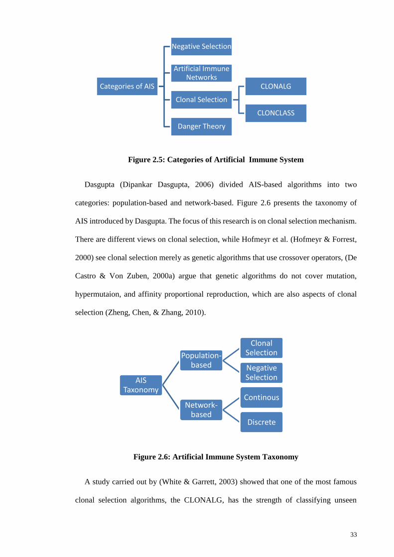
33
Figure 2.5: Categories of Artificial Immune System
Dasgupta (Dipankar Dasgupta, 2006) divided AIS-based algorithms into two
categories: population-based and network-based. Figure 2.6 presents the taxonomy of
AIS introduced by Dasgupta. The focus of this research is on clonal selection mechanism.
There are different views on clonal selection, while Hofmeyr et al. (Hofmeyr & Forrest,
2000) see clonal selection merely as genetic algorithms that use crossover operators, (De
Castro & Von Zuben, 2000a) argue that genetic algorithms do not cover mutation,
hypermutaion, and affinity proportional reproduction, which are also aspects of clonal
selection (Zheng, Chen, & Zhang, 2010).
Figure 2.6: Artificial Immune System Taxonomy
A study carried out by (White & Garrett, 2003) showed that one of the most famous
clonal selection algorithms, the CLONALG, has the strength of classifying unseen
Categories of AIS
Negative Selection
Artificial Immune Networks
Clonal Selection
CLONALG
CLONCLASS
Danger Theory
AIS Taxonomy
Population-based
Clonal Selection
Negative Selection
Network-based
Continous
Discrete

34
patterns, however its learning time is not suitable for time dependent problems and the
authors presented an improved version of this algorithm, dubbed as CLONCLAS, which
was able to reduce the number of generations. They argued that the reason for this poor
performance of CLONALG is that it starts with a global search and then moves to a
random local search and CLONALG uses only one of the mutated clones and discards
the rest, although other high affinity candidates may still exist in the population. However,
their method uses a direct walk in the search space for each example in order to optimize
the population and in contrast to CLONALG, CLONCLAS tries to preserve a larger
proportion of the matured population (White & Garrett, 2003).
Immune algorithms have also become popular for one of their capabilities, namely
solving multi-objective optimization problems because they use population-based
heuristics and these algorithms make possible to handle a set of potential solutions
simultaneously, whereby solutions are the population. These algorithms can find several
members of the Pareto set in a single run of the algorithms, and in contrast to common
mathematical programming methods, they do not need to perform a series of separate
runs and they are also less susceptible to the continuity and shape of the Pareto front
(Villalobos-Arias, Coello, & Hernández-Lerma, 2004). Villalobos-Arias et al.
(Villalobos-Arias et al., 2004) introduced a general mathematical framework to proof that
an entire family of artificial immune algorithms are convergent and eliminated the need
for proving the convergence of each algorithm separately (Timmis, Hone, Stibor, &
Clark, 2008).
One of the most used algorithms for anomaly detection is the negative selection
algorithm (Timmis et al., 2008). One of its strength is the ability of using only a single
class for training the data; however, investigations have shown that a second class is

35
required for tuning the system. Drawbacks of the negative selection algorithm are: high
false positive rate, scaling- and complexity issues (Hart & Timmis, 2008).
A study conducted by Kim et. al (J. W. Kim et al., 2007) emphasized the need for
further investigation into immune algorithms to verify whether or not the incorporation
of up-to-date immunological findings in immune algorithms will ensure real advantages.
2.4 Biologically-based Classification
Although there have been relentless advances in computing technologies, scientist are
still humbled by the sophistication, adaptability and variety of the natural world. (Turing,
1950) one of the pioneers in computational science asked whether computers could think.
From the beginning of the computing technologies, many computational scientists have
been arguing in favour of creating more efficient and faster algorithms, which exhibit
centralized control, while others have been arguing in favor of creating robust, and
adaptable algorithms and less emphasise on efficiency and speed. The latter approaches
has led to biologically inspired computing (Bongard, 2009). One of the strength of bio-
inspired algorithms, was shown by Giles (Giles, 2005); he has shown that Wikipedia,
with low centralized editorial control, is almost as accurate as Encyclopedia Britannica
(Giles, 2005). Although not strictly bio-inspired, Wikipedia uses swarm intelligence
principles (Leitão, Barbosa, & Trentesaux, 2012) to improve the itself with little direction
from above. However, bio-inspired computing does not guarantee performance in clearly
defined domains. Bio-inspired algorithms’ strengths lie in their flexibility; they perform
well when the task is poorly defined; they are able to adapt to unanticipated amendments
in the job environment (Bongard, 2009).
Jerne (Jerne, 1974) introduced the immune network theory (INT), according to his
theory: immune system uses feedback mechanism to maintain a network of cells that are
capable of learning and maintaining memory. In other words, something that has been

36
learnt can be forgotten, unless other parts of the network reinforce it. Perelson (Perelson,
1989) who was motivated by the work of Jerne used the idea of shape space to introduce
criteria for assessing the completeness and overlap in the antibody repertoire. He also
suggested that the immune system is stable but not too stable.
Cooke et al. (Cooke & Hunt, 1995) were inspired by the INT (Perelson, 1989) and
developed an human immune system based Artificial Immune System (AIS). Immunity-
based techniques are a branch of artificial intelligence (Dipankar Dasgupta, Ji, &
Gonzalez, 2003), and thus AIS is a branch of artificial intelligence (Polat, Şahan, &
Güneş, 2006). De Castro et a. (De Castro & Timmis, 2002b) have shown that AIS is
another computational intelligence (CI) paradigms which are systems that can adapt their
behavior so that they can reach their goals which is to solve a particular problem, in a
range of environments (De Castro & Timmis, 2002b). CI describes techniques that focus
on strategy and outcome. CI covers not only AIS, but also Evolutionary Computation,
Particle Swarm Optimization, Ant Colony Optimization, Artificial Neural Networks, and
Fuzzy Systems (Brownlee, 2011). Cooke et al. (Cooke & Hunt, 1995) described how to
use AIS to evolve antibodies that are capable of classifying DNA sequences. Figure 2.7
shows main divisions within computational intelligence.

37
Figure 2.7: Major Groups of Computational Intelligence
(Timmis et al., 2000) used the concept of INT to present the AIS, a primarily
unsupervised machine learning method with the goal of providing the basis for a data
analysis tool. They proposed a network of B cells (the population) where the primary
stimulus was the similarity between the B cell and the pathogen, and the secondary
stimulus for a B was the similarity of the particular B cell to its connected neighbors. The
affinity (the Euclidean distance) is normalized in the range of [0, 1] and the stimulation
is equal to 1 minus the affinity. This means when the distance decreases, the stimulation
effect of the pathogen on the B cell will increase (Timmis et al., 2000). The proposed AIS
uses a fixed mutation rate to clone and mutate B cells in order to construct a memory of
B cells that are able to recognise similar patterns to the one that caused the cloning
(Timmis et al., 2000). AIS consists of nodes and the links between them, which represent
the similarity between the B cells. Timmis et al. defined network affinity threshold (NAT)
as the average affinity associated with all the links in the network. Links between two
cells are created if their affinity exceeds the NAT. Timmis et al. concluded that their
networks were effective for clustering and visualization of the data (Timmis et al., 2000).
Computational Intelligence
Artificial Immune System
Evolutionary Computing
Particle Swarm Optimization
Ant Colony
Artificial Neural Network
Fuzzy Systems

38
The main problem with the immune network theory based artificial immune system
was that it suffered from a population explosion (Brownlee, 2005). After extensive testing
of the AIS, Timmis et al. (Timmis & Neal, 2001) identified this problem and proposed a
new mechanism to control the population. Figure 2.8 shows algorithms that were
developed based on the AIS.
Figure 2.8: Major Derivatives of Artificial Immune System
The new system, which extended the AIS, was dubbed as a Resource Limited Artificial
Immune System (RLAIS). RLAIS is able to limit the size of networks, and allows for
termination conditions to be set, once RLAIS identifies a strong pattern, the network does
not lose or deteriorate the pattern (Timmis & Neal, 2001). For this new system Timmis
et al. introduced the concept of an Artificial Recognition Ball (ARB) which represents a
number of identical B cells; here, only a pre-defined number of B cells are allowed to
exist, which the ARBs’ must compete for. The higher the stimulation level of the ARB,
the more B cell resources an ARB can allocate, and vice versa. Should an ARB loses all
of its B cell resources it becomes unsuitable for learning and will be removed from the
network. In the case that the amount of consumed resources exceeds the amount of
available resources in the system, resources have to be removed from the B cells. In order
to remove these, the least stimulated (the weakest) resource is removed first, the process
of removal of resources continues until there is no difference between the amount of
AIS
RLAIS
ARB
CSA
Immunos81
AIRS
39
allocated resources to all B cells and the maximum amount allowed. Further modification
to the AIS is that the NAT is kept constant by calculating it once at the start of the training
(Timmis & Neal, 2001).
De Castro and his colleague (De Castro & Von Zuben, 2000a) used two biological
principles namely the clonal selection concept and the affinity maturation process to
develop a new technique called the Clonal Selection Algorithm (CSA), it was an
extension to the work of (Jerne, 1974) that was then applied to data clustering. Authors
showed that CSA was able to learn and solve complex problems, it was also highly
parallel and computational cost were manageable (De Castro & Von Zuben, 2000a).
Researchers (De Castro & Von Zuben, 2002) renamed CSA to CLONALG. This
evolutionary algorithm uses clonal selection and affinity maturation principles of the
immune system to do machine-learning and pattern-recognition tasks. since the algorithm
is capable of doing parallel search, after its adaptation, it can be used to solve optimization
problems, authors also showed that CLONALG is capable of doing multimodal search,
their empirical results also showed that it was able to outperform a fitness sharing
technique by locating a higher number of local optima, including the global maximum
(De Castro & Von Zuben, 2002). In a subsequent work De Castro et al. (De Castro & Von
Zuben, 2000b) used genetic variation and selection strategy within a population of
individuals to control the network dynamics and plasticity and named the proposed
method aiNet. In this network clonal selection is used to control the amount and locations
of the cells within the network, and the structure of the final network is defined through
a minimal spanning tree (De Castro & Von Zuben, 2000b). The main goal for developing
aiNet was to solve data analysis problems and authors have successfully applied it to
several data compression and clustering applications (De Castro & Von Zuben, 2001). In
order to perform multimodal optimization tasks, aiNet was further developed by (De
Castro & Timmis, 2002a); empirical results showed that if there is a relative separation

40
between the clusters, aiNet could be used to solve non-linearly separable problems using
a minimal spanning tree of a trained network. Authors also identified many similarities
between their model and the artificial neural networks (De Castro & Timmis, 2002a).
The history of supervised learning system (classification) using immune system
principles starts with the work of Carter (Carter, 2000) when he introduced the Immunos-
81. Carter used abstractions of T cells, B cells, antibodies as well as their interactions to
develop his classifier. This classifier uses artificial T cells to control the formation of B
cell populations, which compete for recognition of “unknowns” (Carter, 2000). Carter
used two standard medical data sets to test the recognition capabilities of the classifier
and achieved good classification results. Carter reported that Immunos-81 were a
powerful, and an easy to build and train classifier. Carter concluded that Immunos-81
offers a viable paradigm for the design of pattern recognition (Carter, 2000).
Watkins’ investigations revealed that there was a lack of research in the arena of
adding a supervised learning component to AIS (Watkins, 2001). The only known
algorithm at that time was the Immunos-81 that was briefly described above. These
investigations lead to the development of Artificial Immune Recognition System (AIRS).
2.5 Research Progress of Hybrid SVM-based Classifiers Within the AIS
Domain
Literature is full with literature related to applications of SVM. In this section, we
briefly introduce research progress of AIS-SVM-based classifiers. For this section we
searched for related articles published either in ISI journals or in important conferences
in the last decade (from 2006 to 2016).
Support vector machine (SVM) is originated from advanced statistical learning theory
(SVMS.org, 2010) it is recognised as a robust and state-of-the-art classification technique.

41
SVM is able to maximize the predictive accuracy of a model without overfitting the
training instances. SVM is mainly suitable for analyzing data with very large numbers of
predictor fields. SVM has found many applications in various disciplines, including bio
sequence analysis, bioinformatics, classification, concept extraction, customer
relationship management, character recognition, text mining, and speech and voice
recognition.
Vapnik et al. introduced SVM in 1995, and later the “soft margin” SVM was presented
by Cortes and Vapnik (Cortes & Vapnik, 1995).
An AIS-SVM hybrid algorithm was developed by (Woolley & Milanović, 2009) for
identifying voltage collapse prone areas and overloaded lines in the power system. In their
study, they used an AIS algorithm to optimize SVM’s parameters. They compared
classification performance of two models, one without optimization- and another one with
optimization of SVM parameters. Their test results showed that the model, which used
AIS to optimize SVM’s parameters, could classify benchmark data sets significantly
better than the standalone SVM model. They have carried out a good study and obtained
good results; however, they did not compare running time of both models, nor did they
report any comparison of their models with other well-known classifiers. It would have
been better to use additional criterion besides the 10-fold cross validation for evaluation of the
models.
Aydin et. al (Aydin et al., 2011) have proposed a model, a hybrid of AIS and SVM.
Here, AIS was used to solve a multi-objective problem for optimizing SVM’s parameters.
They have tested their model against two data sets, one for fault diagnosis, and another
one for anomaly detection. They have achieved good results with their model; however,
they only used cross-validation method to measure the performance of their model. More
evaluation measurements could support their results.

42
Antunes et. al (Antunes, Silva, Ribeiro, & Correia, 2011a; Antunes et al., 2011b)
developed an ensemble of SVM and AIS for classifying text. Their model was applied on
Reuters-21578 data set, and they have achieved good results; however, they did not report
the running time of their models, nor did they compare their model with other available
classifiers.
A hybrid of AIS and particle swarm optimization was introduced by Kuo et. al (Kuo,
Chen, Liao, & Tien, 2013). Their aim was to use this hybrid model in order to optimize
parameters of SVM. They proposed three models: HIP-SVM, AIS-SVM, and PSO-SVM.
These models were applied on six different data sets. The first two models performed
better than PSO-SVM, and both achieved same results with 5 data sets, and only in one
case HIP-SVM performed slightly better than AIS-SVM. Their methodology and results
are very good; however, they did not compare their model with other classifiers. It would
have been better to use additional criterion besides the 10-fold cross validation for evaluation of
the models.
2.6 Artificial Immune Recognition System
AIRS belongs to the field of Artificial Immune Systems, and thus, to the field of
computational intelligence (Brownlee, 2011), and more broadly to the field of artificial
intelligence, this relationship was discussed earlier. AIRS is a clonal selection type of
immune inspired supervised learning algorithm that was introduced by Watkins (Watkins,
2001) who was inspired by the work of (Timmis & Neal, 2001) and was also motivated
by the work of (De Castro & Von Zuben, 2000b). Initially, it was known as AIRS
however, later it was referred to as AIRS1. Based on the experience gained from the
AIRS1, Watkins and Timmis decided to refine the process of the AIRS1 by reducing the
complexity of AIRS1’s approach while maintaining the accuracy of results, and
introduced AIRS2 (Brownlee, 2011). Watkins et al. showed that the AIRS2 is simpler
43
and computationally more efficient than AIRS1 (Watkins & Timmis, 2002, 2004). The
clonal selection theory was introduced by (Burnet, 1959).
Subsection 2.3 briefly introduced relevant aspects of human immune system that have
been utilized as motivation for developing AIS and AIRS. Some key terms that were
discussed before are highlighted next.
B- and T-cells have an exclusive type of molecular receptors which represent locations
in a shape space. The Shape space is defined as the attributes’ features of the antigens.
These receptors enable binding of antigens and antibodies, the higher the affinity between
them the stronger the binding. The affinity is defined as the degree of similarity between
antigens and B-cells. The Euclidean distance is one of the methods that can be used to
measure the affinity which represent the interaction between elements. Antigenic
presentation is another name for antigen/antibody binding; in AIRS it refers to matching
between antigens (training data) and B-cells (potential solutions) (Watkins, 2005). As
mentioned in subsection 2.4, the ARB represent a number of identical B cells (Timmis et
al., 2000) and it reduces duplication as well as dictates survival within the population
(Watkins, 2005). Affinity maturation is a learning process of the immune system; this
process involves determining the affinity between an antigen and a B-cell and
transforming the involved B-cell into a plasma cell (Watkins, 2005). During an immune
response the recognition B-cell will undergo rapid clonal expansion in proportion to how
well it matches the antigen; the goal is to generate as many clones of itself so that the next
time it sees an antigen, it matches the antigen better. This response is antigen specific.
The generated clones then undergo a process called somatic hypermutation proportional
to the affinity between the B-cell and the antigen (Brownlee, 2005; Watkins, 2005). The
generated clones have different features (receptors) than their parent; therefore it is
possible that some of them are a better match to the antigen observed and since only those
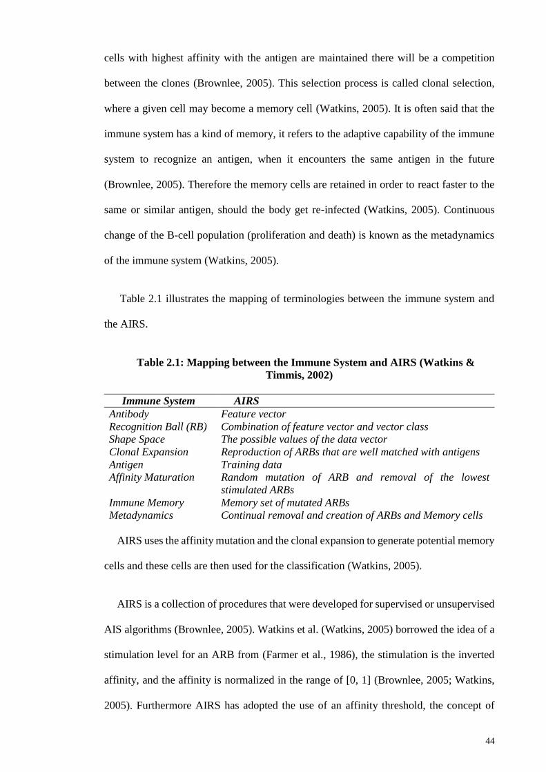
44
cells with highest affinity with the antigen are maintained there will be a competition
between the clones (Brownlee, 2005). This selection process is called clonal selection,
where a given cell may become a memory cell (Watkins, 2005). It is often said that the
immune system has a kind of memory, it refers to the adaptive capability of the immune
system to recognize an antigen, when it encounters the same antigen in the future
(Brownlee, 2005). Therefore the memory cells are retained in order to react faster to the
same or similar antigen, should the body get re-infected (Watkins, 2005). Continuous
change of the B-cell population (proliferation and death) is known as the metadynamics
of the immune system (Watkins, 2005).
Table 2.1 illustrates the mapping of terminologies between the immune system and
the AIRS.
Table 2.1: Mapping between the Immune System and AIRS (Watkins &
Timmis, 2002)
Immune System AIRS
Antibody Feature vector
Recognition Ball (RB) Combination of feature vector and vector class
Shape Space The possible values of the data vector
Clonal Expansion Reproduction of ARBs that are well matched with antigens
Antigen Training data
Affinity Maturation Random mutation of ARB and removal of the lowest
stimulated ARBs
Immune Memory Memory set of mutated ARBs
Metadynamics Continual removal and creation of ARBs and Memory cells
AIRS uses the affinity mutation and the clonal expansion to generate potential memory
cells and these cells are then used for the classification (Watkins, 2005).
AIRS is a collection of procedures that were developed for supervised or unsupervised
AIS algorithms (Brownlee, 2005). Watkins et al. (Watkins, 2005) borrowed the idea of a
stimulation level for an ARB from (Farmer et al., 1986), the stimulation is the inverted
affinity, and the affinity is normalized in the range of [0, 1] (Brownlee, 2005; Watkins,
2005). Furthermore AIRS has adopted the use of an affinity threshold, the concept of

45
ARB and population control mechanism from AINE (Thomas Knight & JonathanI
Timmis, 2001; Watkins, 2005) and borrowed random mutation, clonal expansion, and
clonal selection from other AIS-based algorithms (Brownlee, 2005), these topics were
introduced and discussed above.
This thesis uses the following definitions of the key terms and concepts that were
introduced by (Watkins, 2001):
Artificial Recognition Ball (ARB) represents a number of identical B-Cells
and is also a mechanism to reduce duplication and dictate survival within the
population (Watkins, 2001).
Affinity threshold scalar (ATS): It is a value between 0 and 1 that when it gets
multiplied by affinity threshold, it provides a cut-off value for memory cell
replacement during training phase (Watkins, 2001).
Clonal rate: It is an integer value that is used to determine the number of
mutated clones a given ARB is allowed to attempt to produce (Watkins, 2001).
Hyper-mutation rate: It is an integer value that is used to determine the
number of mutated clones that a given memory cell is allowed to inject into the
cell population (Watkins, 2001).
Seed cell: It represents an antibody that is drawn from the training set and is
used to initialize Memory Cell and ARB populations at the beginning of
training (Watkins, 2001).
Stimulation value: It is the value returned by the stimulation function, this
function is used to measure the response of an ARB to an antigen or to another
ARB. The function returns a value between 0 and 1 (Watkins, 2001).
Total resources: It is a parameter which sets limitations on the number of
ARBs allowed in the system. Each ARB is allocated a number of resources
based on its stimulation value and the clonal rate (Watkins, 2001).
In general, the goal of developing AIRS algorithm was setting memory cells that can
be used for data classification. These artificial memory cells represent a number of
features of the immune systems. They represent memory B cells that have gone through
a maturation procedure in the human body.
Each ARB is represented by an n dimensional vector and a class to which the data
belongs. Furthermore each ARB is assigned a stimulation value that is calculated through
Equation 2.2, where x is feature vector of the ARB, and y is the training antigen; AIRS
uses the Euclidean distance to measure the affinity (Watkins, 2005):Function

46
𝑎𝑓𝑓𝑖𝑛𝑖𝑡𝑦 (𝑥, 𝑦) = 1 − 𝐸𝑢𝑐𝑙𝑖𝑑𝑒𝑎𝑛 𝐷𝑖𝑠𝑡𝑎𝑛𝑐𝑒 (𝑥, 𝑦) = 1 − √∑(𝑥𝑖 − 𝑦𝑖)2𝑛
𝑖=1
(2.1)
𝑆𝑥 = {1 − 𝑎𝑓𝑓𝑖𝑛𝑖𝑡𝑦 (𝑥, 𝑦): 𝑖𝑓 𝑥 𝑎𝑛𝑑 𝑦 ℎ𝑎𝑣𝑒 𝑡ℎ𝑒 𝑠𝑎𝑚𝑒 𝑐𝑙𝑎𝑠𝑠
𝑎𝑓𝑓𝑖𝑛𝑖𝑡𝑦 (𝑥, 𝑦): 𝑖𝑓 𝑐𝑙𝑎𝑠𝑠 𝑜𝑓 𝑥 𝑎𝑛𝑑 𝑦 𝑎𝑟𝑒 𝑑𝑖𝑓𝑓𝑒𝑟𝑒𝑛𝑡
(2.2)
The smaller the Euclidean distance, the higher the affinity and higher affinity means
generating larger number of clones. The affinity threshold is the average Euclidean
distance between each instance in the training data set; cells with the highest affinity are
selected for cloning and are ultimately used for creating an established memory set; how
many clones are created depends on their antigenic affinity in other words, how well they
match; in order to create diversity, ARBs also experience a random mutation (Watkins,
2005).
Figure 2.9 illustrates the outline of AIRS2’s algorithm. Algorithm AIRS2 consists of
four stages to learning: 1) initialization, 2) memory cell identification, 3) resource
competition, and 4) refinement of established memory cells (Watkins, 2005). In the first
stage data is normalized and initialized so that the affinity of every two training records
is in the range of [0, 1]. In this stage, there is an option for seeding the memory cell pool.
This pool represents a collection of recognition elements that form the classifier which is
produced at the end of training phase. Initialization stage also calculates affinity threshold
which is used during training phase to determine whether prepared candidate memory
cells can replace already existing memory cells in the classifier (Watkins et al., 2004).

47
Figure 2.9: Outline of AIRS2 (Watkins, 2005)
Figures 2.10 through 2.17 illustrate the process of AIRS algorithm. As mentioned
earlier the goal is to generate recognition elements (records or feature vectors) that can
be used to classify new instances at the end of training scheme. These recognition
elements are collected in the memory cell pool. Initially the memory cell pool is empty
and optionally can be seeded with few randomly selected records from the training data.
The letter “A” in the circle represents an instance from the training data, for which the
algorithm is going to generate recognition vectors.
The incoming training data items (records) represent antigens and the items that will
be generated in the memory cell pool represent the antibodies also known as B cells which
are obviously also vectors. The AIRS algorithm determines the affinity threshold (AT)
which is the mean affinity between antigens (records) in the training dataset. This value
is used later during the training phase to verify whether existing memory cells can be
1. Compare a training instance with all memory cells of the same class and
find the memory cell with the best affinity for the training instance. Refer
to this memory cell as 𝑚𝑐𝑚𝑎𝑡𝑐ℎ
2. Clone and mutate 𝑚𝑐𝑚𝑎𝑡𝑐ℎ in proportion to its affinity to create a pool
of abstract B-Cells
3. Calculate the affinity of each B-Cell with the training instance
4. Allocate resources to each B-Cell based on its affinity.
5. Remove the weakest B-Cells until the number of resources returns to a
preset limit.
6. If the average affinity of the surviving B-Cells is above a certain level,
continue to step 7, Else clone and mutate these surviving B-Cells based
on their affinity and return to step 3.
7. Choose the best B-Cells as a candidate memory cell (𝑚𝑐𝑐𝑎𝑛𝑑)
8. If the affinity of 𝑚𝑐𝑐𝑎𝑛𝑑 for the training instances is better than the
affinity of 𝑚𝑐𝑚𝑎𝑡𝑐ℎ , then add 𝑚𝑐𝑐𝑎𝑛𝑑 to the memory cell pool. If, in
addition to this, the affinity between 𝑚𝑐𝑐𝑎𝑛𝑑 and 𝑚𝑐𝑚𝑎𝑡𝑐ℎ is within a
certain threshold, then remove 𝑚𝑐𝑚𝑎𝑡𝑐ℎ from the memory cell pool.
9. Repeat from step 3 until all training instances have been presented.
When the training routine is completed, AIRS uses kNN to classify
instances with the developed set of memory cells (Watkins, 2005).

48
replaced with candidate memory cells which are prepared. Affinity represents the
similarity between records (vectors), the higher the affinity the more similar are the
vectors (Brownlee, 2005; Watkins, 2001).
The AIRS algorithm is a single-shot algorithm, meaning it only needs to pass once
over the training data to prepare the classifier. One at a time, each record is exposed to
the memory cell pool (Brownlee, 2005; Watkins, 2001).
Figure 2.10 shows the initial phase of the algorithm when an instance “A” is presented
to the memory cell pool from where a matching record is sought. The vectors (cells) in
the memory cell pool are stimulated by the record “A” and each vector in the memory
cell pool is assigned a stimulation value. The stimulation value is given through the
Equation 2.2.
Figure 2.10: Memory Cell Identification
The AIRS2 algorithm uses the Euclidean distance as the primary metric for both
affinity and stimulation, however other functions could also be used (Watkins, 2001). The
vector with the greatest stimulation is selected as best match memory cell and is used in
the affinity maturation process (Brownlee, 2005; Watkins, 2001).

49
Figure 2.11 illustrates the situation when a matching record is found and is marked as
the MCmatch.
Figure 2.11: Identifing MCmatch
Figure 2.12 shows the process of generating new ARBs (vectors) which are a number
of mutated clones of the MCmatch that are added into the population (ARB pool).
Figure 2.12: Process of Generating ARBs
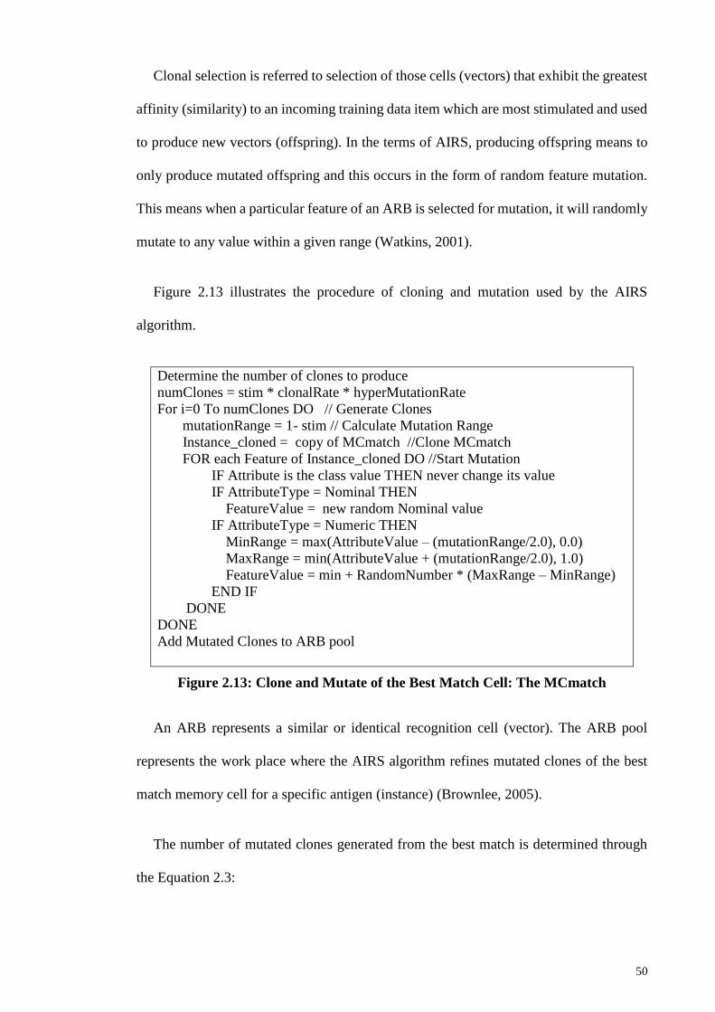
50
Clonal selection is referred to selection of those cells (vectors) that exhibit the greatest
affinity (similarity) to an incoming training data item which are most stimulated and used
to produce new vectors (offspring). In the terms of AIRS, producing offspring means to
only produce mutated offspring and this occurs in the form of random feature mutation.
This means when a particular feature of an ARB is selected for mutation, it will randomly
mutate to any value within a given range (Watkins, 2001).
Figure 2.13 illustrates the procedure of cloning and mutation used by the AIRS
algorithm.
Determine the number of clones to produce
numClones = stim * clonalRate * hyperMutationRate
For i=0 To numClones DO // Generate Clones
mutationRange = 1- stim // Calculate Mutation Range
Instance_cloned = copy of MCmatch //Clone MCmatch
FOR each Feature of Instance_cloned DO //Start Mutation
IF Attribute is the class value THEN never change its value
IF AttributeType = Nominal THEN
FeatureValue = new random Nominal value
IF AttributeType = Numeric THEN
MinRange = max(AttributeValue – (mutationRange/2.0), 0.0)
MaxRange = min(AttributeValue + (mutationRange/2.0), 1.0)
FeatureValue = min + RandomNumber * (MaxRange – MinRange)
END IF
DONE
DONE
Add Mutated Clones to ARB pool
Figure 2.13: Clone and Mutate of the Best Match Cell: The MCmatch
An ARB represents a similar or identical recognition cell (vector). The ARB pool
represents the work place where the AIRS algorithm refines mutated clones of the best
match memory cell for a specific antigen (instance) (Brownlee, 2005).
The number of mutated clones generated from the best match is determined through
the Equation 2.3:

51
numClones = stim * clonalRate * hypermutationRate (2.3)
where the stim is the stimulation value between the best match memory cell (Vector) and
the antigen (the instance “A”). The values for other two parameters, the clonalRate and
the hypermutationRate are defined by the user (Brownlee, 2005; Watkins, 2001).
Figure 2.14 represents the process of competition for system wide resources and the
use of mutation for diversification and shape-space exploration as well as the use of
average stimulation threshold as a criterion for determining when to stop training on a
given antigen (instance) (Brownlee, 2005; Watkins, 2001).
Figure 2.14: Process of Resource Allocation and Competition
Training for an antigenic pattern has to stop at some time, therefore the algorithm
verifies whether or not ARBs have been stimulated enough for the training, the algorithm
uses the average stimulation values for the ARBs of each class as termination condition,
if each of these averages becomes greater than a pre-defined threshold the training ends
for that particular pattern (Watkins, 2005; Watkins et al., 2004).

52
In the third stage the algorithm handles competition for resources during development
procedure of a candidate memory cell. The goal of this stage is to develop a memory cell
that is most successful in accurately classifying a given antigen. To achieve this goal the
algorithm uses three mechanisms. The first mechanism is about system wide resource
competition. A number of mutated clones of the best matching memory cell MCmatch
are added to the ARB pool and the process of generation of recognition vectors and
competition starts. The process of competition is necessary for controlling the size of the
ARB pool as well as promoting those ARBs that have greater affinity (stimulation) to the
antigen (instance) being trained on (Brownlee, 2005). This process considers only ARBs
of the same class as the antigen (the instance). The flow chart of this process is illustrated
in Figure 2.15 (Brownlee, 2005):
Figure 2.15: Flow Chart for Resource Allocation and Competition of AIRS
Generate mutated clones of surviving ARBs
Stimulate ARB pool with antigen (instance)
Normalize ARB stimulation values
Allocate limited Resources based on
Prune ARBs with insufficient resources
Stop Stop

53
Then the algorithm uses the same clonal expansion and hypermutation as it has used
to generate mutated clones of the best match memory cell MCmatch, to mutate each ARB
in the pool. Equation 2.4 used to determine the number of clones for each ARB in the
pool (Brownlee, 2005).
numClones = stim * clonalRate (2.4)
In order to allocated resources, Watkins (Watkins, 2001) followed the methods that
were outlined by (Timmis et al., 2000) and enhanced by (Thomas Knight & Jonathan
Timmis, 2001). Resource allocation is based on the stimulation value which indicates the
fitness of the recognizer (Watkins, 2001). Normalized stimulation value of the ARB
indicates the fitness of ARB that will become a recognizer of an antigen. This value is
used to determine the amount of resource allocation. A user defines the maximum amount
of resources to be allocated, and the number of resources allocated to each ARB is
determined through the Equation 2.5:
resource = normStim * clonalRate (2.5)
where normStim is normalized stimulation value and clonalRate is the clonal Rate. The
second mechanism uses mutation for shape-space search and divergence.
Marwah and Boggess (Marwah and Boggess 2002) allocated resources differently;
they assigned more resources to the antigen classes that occurred more frequently. AIRS2
as well as Marwah’s proposed algorithm use linear resource allocation, and because of
this linearity the algorithms need longer time for classification and require higher number
of memory cells (Golzari, Doraisamy, Sulaiman, & Udzir, 2008; Polat, Şahan, Kodaz, et
al., 2007).
The third mechanism defines the stopping condition whereby this condition depends
on the average of stimulation threshold (Watkins et al., 2004). Production of ARBs
54
continues until the stopping criteria are met, and then the candidate memory cell is
selected based on its stimulation value and class. The candidate memory cell is the one
with the maximum stimulated ARB of the same class as the antigen (Watkins, 2005;
Watkins et al., 2004).
In the process of resource allocation the total resources allocated by all ARBs is
determined and compared to the allowed maximum total resources.
Then the ARB pool is sorted by allocated resources in descending order, if the total
resources allocated is greater than the maximum allowed resources, then resources are
removed from ARBs starting at the end of the list (from the weakest thus least stimulated
ARBs) until the total allocated resources fall below the maximum allowed resources.
If an ARB’s resource becomes zero, it will be removed from the ARB pool. The
process of refinement of ARB has a stopping condition which occurs when the mean
stimulation becomes greater than the stimulation threshold that is given by the user
(Brownlee, 2005; Watkins, 2001).
Figure 2.16 illustrates the process of comparing response of MCmatch and
MCcandidate to the antigen and comparison of the affinity value of MCmatch and
MCcandidate to each other.
When the refinement process of the ARB is completed, the ARB with the greatest
stimulation value is selected as a memory cell candidate MCcandidate (Brownlee, 2005).
In the fourth stage of the algorithm the potential candidate memory cell is introduced
into the set of already established memory cells for training.

55
Figure 2.16: Development of MCcandidate and Resource Competition
Figure 2.17 illustrates the process of introducing the just-developed candidate memory
cell (vector), the MCcandidate, into the set of existing memory cells MC.
Figure 2.17: Introduction of Memory Cell to Memory Cell Pool

56
If MCcandidate’s stimulation value is higher than that of the original best matching
memory cell, MCcandidate will be added into the memory cell pool (Brownlee, 2005).
Then the algorithm verifies if MCmatch can be replaced by MCcandidate; this happens
when the affinity between the MCcandidate and the best matching cell is less than a cut-
off. The cut-off is given by the following Equation 2.6:
cutOff = affinityThreshold * affinityThresholdScalar (2.6)
where the affinityThreshold is the variable that was prepared during the initialisation
phase of the algorithm, and the affinityThresholdScalar is a user defined parameter
(Brownlee, 2005).
The above process repeats until all antigens (that is: all instances of training data set)
have been introduced to the system (Watkins et al., 2004). After the training process is
completed the evolved memory cells in the memory cell pool are available for use for
classification. AIRS uses a k-Nearest Neighbor classifier to perform the classification
task, here the k-best matches to data instances are identified and via majority vote the
class is determined (Brownlee, 2005).
2.6.1 Differences between AIRS1 and AIRS2
As mentioned above AIRS1 was the first version of AIRS, detailed explanation of this
algorithm was given by (Watkins, 2001). Differences between the AIRS1 and the AIRS2
are explained next.
Somatic hypermutation (affinity proportional mutation) is used by the majority of AIS
techniques; however AIRS1 did not use this metaphor, instead it used a naïve random
generation of mutations (Watkins, 2005). AIRS1 maintained two independent pools of
cells, namely the ARB pool and the memory cell pool. The ARB pool was used to evolve
a candidate memory cell belonging to the same class as the training antigen, and at the

57
same time AIRS1 maintained ARBs of other classes which were taken care of previously
(Watkins, 2005). All these ARBs participated in the competition for the limited resources
and as a result the algorithm would need more time for rewarding and refining those
ARBs that have the same class as the concerned antigen (Brownlee, 2005). Through
animated analysis of the ARB pool Watkins et al. figured out that the effort to evolve
ARBs of a different class than the training antigen was useless, and they concluded that
a good potential memory cell must have the same class label as the training antigen
(Watkins, 2005). This led to the elimination of maintaining multiple classes in the
memory of system (“resource management of AIRS2”) and thus improving the overall
runtime and a simplification of AIRS2 algorithm (Watkins, 2005).
AIRS1 used to generate clones of multiple classes however only clones of the same
class as the antigen are used in the ARB pool (Brownlee, 2005), AIRS2 maintains only
the ARBs of the same class and does not allow mutation of the class value (switching
classes are not permitted) this is in contrast to how AIRS1 dealt with ARBs (Watkins,
2005).
While in AIRS1 a user has the ability to set the “mutate rate” parameter to control the
degree to mutate a created clone, AIRS2 uses the notion of somatic hypermutation where
the quantity of mutation of a produced clone is proportional to its affinity to the
concerning antigen (Brownlee, 2005).
Evaluation results showed that classification accuracy of both AIRS1 and AIRS2 was
similar, however AIRS2 is simpler and has better computation performance and provides
improved data reduction of the training instances (Brownlee, 2005).
Details about the differences between the AIRS1 and the AIRS2 can be found in
(Watkins & Timmis, 2002).

58
2.6.2 AIRS in the Literature
Applications of AIRS1 on various benchmark classification problems revealed that its
performance was as good as other well-respected supervised learning techniques for equal
benchmarks (Watkins & Boggess, 2002).
Goodman et al. studied the behaving manner of AIRS on many publicly existing
classification problems. While keeping the number of features constant, they incremented
the number of classes, and they compared the obtained results with a well-known
classifier, the Kohonen's Learning Vector Quantization (LVQ). They showed that average
performance of AIRS on one of the problems was even the best for that particular problem
(Goodman et al., 2002). Under the condition of similar number of elements, AIRS
outperformed both LVQ and an optimized version of the LVQ in almost all cases for the
real-world classification problems (Brownlee, 2005). Goodman et al. did a valuable
evaluation of AIRS; however, a comparison with only one classifier, the LVQ, is not adequate
for determining the performance’s quality of AIRS. It would have been better to use additional
criterion besides the 10-fold cross validation for evaluation of the models.
In another research, Goodman et al. also investigated AIRS empirically. They
exchanged one of the two potential sources of its classification strength with another
modifications. They concluded that outcomes were marginally less effective, however it
was statistically insignificant. The modifications delivered quick test version of AIRS.
They compared AIRS’s performance with other best classifiers on the same multiple-
class problems and demonstrated that AIRS was competitive with top classifiers. They
showed that the mechanism for replacement and maintenance of AIRS’ memory cell
population is the source of AIRS’ classification power. (Goodman, Boggess, & Watkins,
2003). Their evaluation method could be more powerful, if they ran other classifiers by
themselves under equal computational circumstances that existed for AIRS. Instead they

59
used the online result of (Duch, 2000). Their evaluation could have included broader
classification tasks (that is: more data sets).
In another study, Marwah et al. (2002) inspected many different algorithms for
situations when two or more classes had equal number of memory cells among the k
strongest stimulated memory cells. Their study revealed that in average, AIRS’ accuracy
was higher for one of the development environment than any reported at the UCI
repository for that environment (Marwah & Boggess, 2002). They have done a great
evaluation of AIRS’ handling of ties, by modifying competition process for resource
allocation of AIRS; however, their methods did not really improve the performance of
AIRS algorithm.
Boggess et al. (Boggess & Hamaker, 2003) studied the effect of adding irrelevant
features to datasets and compared classification accuracies obtained from AIRS and LVQ,
their result showed that LVQ outperformed AIRS when prepared with the equal number
of codebook vectors discovered by AIRS; however, LVQ was not able to outperform
AIRS when it was configured independently (Brownlee, 2005).
Meng et al. did a comprehensive benchmark experiment on AIRS, and have concluded
that results of AIRS were reasonable and it could be used for real-world classification
tasks (Meng et al., 2005). They used two versions of AIRS: AIRS-1 and AIRS-7;
however, they did not mention what their differences are. They also did not provide the
values for the parameters of either AIRS algorithms, and it would have been better to use
additional criterion besides the 10-fold cross validation for the evaluation of proposed algorithms.
Hamaker et al. studied how using non-Euclidean distance measures affects the
classical AIRS algorithm; they used four well-known classification problems with
numerous amounts of real, nominal, and discrete features. Their study showed the need

60
for further research into non-Euclidean distance measure that performs best for a
particular data set (Hamaker & Boggess, 2004). Their results revealed that AIRS can
obtain better classification accuracy, if more natural and useful measure of comparison is
used (Brownlee, 2005). Hamaker & Bogges (2004) have carried out an extensive
investigation into the rule of various distance measures in AIRS; however, they did not
discuss whether their results were statistically significant different from the traditional
AIRS.
Polat et al. incorporated fuzzy logic into resource allocation procedure of AIRS in
order to improve classifer’s performance. They reasoned that long running time,
excessive resource allocation, and high number of memory cells of classical AIRS are
due to the linearity of resource allocation procedure. Their method accomplished higher
classification accuracy than various well-known classifiers on the same data sets (Polat
& Güneş, 2008). Although they have achieved a very good result with their hybrid
algorithms, however their report did not show how much “fuzzy resource allocation”
contributed to the success of the algorithm.
Golzari et al. introduced real-world tournament selection procedure inside resource
competition part of AIRS1 and achieved higher classification accuracy than other
benchmark classifiers including the AIRS1. They argued that during competition stage of
AIRS1, high selection pressure is the reason for loss of diversity and this may produce
premature memory cells. They reported that their method achieved significantly higher
classification accuracy than AIRS1 in all cases on the benchmark datasets from the UCI
machine learning repository (Golzari et al., 2009a, 2009b). They have achieved very good
results with AIRS1; however, they did not report whether the use of RWTS would also
improve the performance of AIRS2.
61
Polat et al. developed a hybrid method involving AIRS and fuzzy weighted pre-
processing; with this method, they classified the thyroid disease dataset. They compared
their result with that obtained from AIRS, and reported their method performed better
than ARIS (Polat, Şahan, & Güneş, 2007). Their result for the thyroid data set is very
good, however they did not discuss why did they use fuzzy weighting pre-processing of
the data set, nor did they report the running time of their algorithm. They did not describe
how they have determined the parameter values for their fuzzy AIRS.
Saidi et al. as well as Chikh et al. argued that k-NN’s classification time depends on
the number of data points that are used. Therefore, in order to reduce memory cell pool
of AIRS2, they introduced fuzzy k-nearest neighbor to assign a class membership to each
instance; they found that reducing number of memory cell pool improves algorithms’
performance. Authors compared their results with the result obtained with AIRS2, and
concluded that their model achieved higher classification accuracy (Chikh et al., 2012;
Saidi, Chikh, & Settouti, 2011). Their proposed method was able to reduce the size of
memory cell pool and at the same time achieve higher classification accuracy than AIRS2.
However, they did not discuss one important issue, namely the running time of their
algorithm and its comparison with that of AIRS2.
Forouzideh et al. presented an application of AIRS for in text-document classification.
In their study, different versions of AIRS were compared with RBF and multi-layer
perceptron (MLP); their results showed that different versions of AIRS classified better
than both RBF and MLP. They expected more successful and diverse applications of
AIRS to emerge in the future, because of its high performance (Forouzideh, Mahmoudi,
& Badie, 2011). They did a good comparison of various versions of AIRS for text mining.
They wrote that they have proposed fuzzy AIRS model, however they didn’t provide the
pseudocode for this model. They have used the fuzzy KNN, which was developed by

62
Keller et. al. (Keller, Gray, & Givens, 1985) in AIRS1, but they did not discuss why they
did not use it in AIRS2.
Another area where researchers have found promising capability for AIRS is
analyzing microarray data (Chen, Xu, Bie, & Gao, 2008). They only used AIRS2 to
classify microarray data sets, and did not introduce any new model.
Le et al. combined E-algorithm with AIRS and created a novel Fuzzy AIRS dubbed as
FAIRS; this new algorithm was used to identify the reason of power outage. Results
obtained with FAIRS, AIRS, and E-algorithms were comparable, however FAIRS was
considerably faster in computing time than E-algorithm (Le & Mo-Yuen, 2008). They
have introduced an interesting algorithm, but converting the antibodies into different
format for representing fuzzy classification rules, seems to be rather complicated. Their
algorithm appears to have been customized for their data set, and their report does not
show how this algorithm would behave on other data sets. Although the results are good,
further investigation into their model and its application with other data sets are still
needed to make a better conclusion.
There are many applications with substantial results in diagnosing several diseases.
Latifoğlu et. al. developed an AIRS-based application to diagnose atherosclerosis. With
a classification accuracy of 99.29%, they concluded that their model could help medical
specialists in diagnosing atherosclerosis patients (Latifoǧlu, Kodaz, Kara, & Güneş,
2007). They have achieved a very good result, and reported classification accuracy,
specificity, and sensitivity, however they did not compare their results with other
available classifiers, and did not report about the running time of their model.
In another study, Kodaz et al. developed an AIRS-based algorithm in order to diagnose
thyroid disease. Their model reached a classification accuracy of 94.82% (Kodaz,

63
Babaoğlu, & İşcan, 2009). They have achieved very good result, however they did not
compare their results with other available classifiers, instead they have presented what
other researchers have reported, and this makes the comparison almost impossible,
because the classifiers were ran under different circumstances.
A hybrid algorithm of fuzzy-weighted pre-processing and AIRS was developed by
Polat et al. for diagnosing heart disease, they classified the disease with an accuracy of
96.3% (Polat, Güneş, & Tosun, 2006). Their result for diagnosing heart disease is very
good, however they did not discuss why did they used fuzzy weighting pre-processing of
the data set, nor did they report the running time of their algorithm. It seems they have
used AIRS1, and they do not report why they did not use AIRS2.
Şahan et al. introduced a hybrid fuzzy-artificial immune system with KNN in order to
classify Wisconsin Breast Cancer Dataset; this hybrid model classified the disease with
an accuracy of 99.14% (Şahan et al., 2007). Their result for diagnosing breast cancer is
very good, however they did not discuss why did they used fuzzy weighting pre-
processing of the data set, nor did they report the running time of their algorithm. It seems
they have used AIRS1, and they do not report why they did not use AIRS2. They did not
compare their model with other available classifiers; instead, they have presented what
other researchers have reported on the same data set. This comparison is not accurate,
since the experiments were ran under different circumstances.
Kara et al. introduced another medical application of AIRS, for classifying
microorganism species, they developed an information gain based AIRS (IG-AIRS) and
reported they classified the species with an accuracy of 92.35% (Kara et al., 2009). The
result of their model was compared with that of other benchmark classifiers; however,
their model was not verified with other datasets, and they only used fivefold cross
validation for evaluation of their model.
64
Shamshirband et al. combined AIRS with fuzzy labeling for diagnosing tuberculosis
disease. Their model classified the disease with an accuracy 99.14% (Shamshirband et
al., 2014). They have achieved a very good result, however they did not compare their
model with other classifiers by themselves. Instead, they have presented what other
researchers have reported on the same data set. This comparison is not accurate, since the
experiments were ran under different circumstances.
In another related study, Lin et al. used AIRS, logistic regression, and SVM to predict
type 2 diabetes among pregnant women. Researchers compared results obtained with
AIRS, SVM, and logistic regression and reported that AIRS achieved highest
classification accuracy among these three classifiers, and that their obtained accuracy was
62.8% on the diabetes data set (Lin, Su, & Wang, 2011). They achieved a good result
with AIRS; however, they did not modify AIRS, and thus did not provide a new model.
Their report does not show any running time of the applied models either.
Sunny et al. showed the robustness of AIRS to identify gases/odors. They compared
the classification performance of AIRS1, AIRS2 and Parallel AIRS to that of Radial Basis
Function Neural Network, Naïve Bayes, and Learning Vector Quantization whereby they
used principal component analysis to reduce the dimensions of the raw data. They
concluded that AIRS-based algorithms performed better than other three classifiers
(Mishra, Dwivedi, & Das, 2013). They achieved good results with different versions of
AIRS; however, they did not modify AIRS, and thus did not provide a new model. Their
report does not show any running time of the applied models either.
Tay et al. were motivated by the capability of AIRS to perform classification and
developed an evolutionary data-conscious AIRS, which was dubbed as EDC-AIRS. Their
model mimics the response of antibodies to the antigens, which depends on the density,
location and type of invaders (antigens). The performance of their model was evaluated
65
on four benchmark data sets and was compared with other classifiers; their model ranked
in the top 3 positions, and outperformed AIRS2 in all cases. Classification accuracies
obtained with EDC-AIRS for Ionosphere, Iris, Sonar, and Pima Indians were 98.0%,
99.6%, 90.9%, and 77.3% respectively (Tay et al., 2013). They have introduced a very
interesting model with very good results; however, they did not report one important
issue, the running time, of their models.
In our study of the literature, we found that the term AIRS has been used by many
researchers, but majority of them did not clearly distinguish whether they refer to AIRS1
or AIRS2. In this thesis however, the focus is to make changes to AIRS2 algorithm. In
this section we have introduced and analyzed AIRS-based models that have been
developed by other researchers. Some of models were built to solve a particular
classification problem and therefor their authors did not verified their model with other
data sets. In order to verify whether these models perform well with other data sets,
additional tests with other data sets are required. In many cases, the authors did not
compare their models with other well-known classifiers. Instead, they presented results
from the literature, these kind of comparisons are not valid, because all of the models ran
under different computing circumstances and not under equal computing conditions. One
important issue was missing in all articles, the running time of the models. It is important
to know, how long a classifier does needs to do the classification.
2.7 Classifiers Used In This Research As Benchmark Classifiers
In this subsection, we introduce classifiers that are used in this research. Some
benchmark classifiers were introduced in previous subsections of this chapter. Names of
all well-known classifiers that are used as benchmark classifiers, in this study, are
presented in subsection 3.4.8.
66
LibSVM stands for library for support vector machines (SVM) that has been actively
developed by Chang et al. (Chang & Lin, 2011). It is popular in machine learning and
other areas. LibSVM has found applications in computer vision (Grauman & Darrell,
2005; Hu et al., 2012), natural language processing (Nivre et al., 2007), neuroimaging
(Hanke et al., 2009), bioinformatics (Dorff, Chambwe, Srdanovic, & Campagne, 2010),
to name few domains. Support vector machines are discussed in detail in subsection 4.3.1.
LibSVM supports: one-class SVM, support vector regression (SVR), and support vector
classification (SVC) for two-class and multiclass cases.
Platt (Platt, 1999) developed an algorithm for training of SVM dubbed as Sequential
Minimal Optimization (SMO). In contrast to SVM that solves large quadratic
programming (QP) optimization problem, SMO first divides these large QP problem into
a series of smallest possible QP problems. By solving these small QP problems
analytically and iteratively, the algorithm bypasses a time-consuming QP optimization.
Since SMO does not use large matrix computation, its training set size for various test
problems scales somewhere between linear and quadratic values (Platt, 1999).
Applications of SMO can be found in (Bach, Lanckriet, & Jordan, 2004; Q. Li, Salman,
Test, Strack, & Kecman, 2013; Zięba, Tomczak, Lubicz, & Świątek, 2014).
The statistician David Cox (Cox, 1958) developed logistic regression, it uses a logistic
function to estimate the probability of the relationship between one or more independent
variables and the categorical dependent variables. The logistic function provides values
between 0 and 1 and that makes the logistic function so popular, because the model
describes a probability that is always somewhere between 0 and 1 (Kleinbaum & Klein,
2010). Logistic regression analysis is a suitable tool for classification problems, however
it is possible to get high misclassification rate (D. Liu, Li, & Liang, 2014). Logistic
regression has found many applications: in linear model and survival analysis (Harrell,

67
2013), in decision making of financial company (Swiderski, Kurek, & Osowski, 2012),
in hyperspectral image classification (Felicísimo, Cuartero, Remondo, & Quirós, 2013),
in classification of breast cancer (M.-L. Huang, Hung, Lee, Li, & Wang, 2012), and many
more.
A multi-layer perceptron (MLP) is known as a feed-forward neural network. It is one
of most widely used version of neural network. MLPs are popular among engineers,
scientists and other professionals. They are used to tackle a wide variety of information
processing tasks. Like all neural networks, multi-layer perceptron are trained to do the
chosen task. One of popular research areas within the field of neural computing is the
development of fast and reliable training algorithms for MLPs (Shepherd, 2012).
Multilayer feedforward neural networks are ideal for handling difficult tasks in pattern
recognition, because its structure is highly adaptable (Strzelecki, Szczypinski, Materka,
& Klepaczko, 2013). MLPs have been successfully used in a wide variety of tasks such
as speech recognition (Siniscalchi, Yu, Deng, & Lee, 2013), image compression (Kalita
& Sarma, 2015), pattern recognition (Chauhan, Goel, & Dhingra, 2012; Dervilis et al.,
2014), features reduction (Phinyomark et al., 2013; Strzelecki et al., 2013), and many
more.
Since the introduction of artificial neural networks in 1990, multilayer neural networks
and radial basis function (RBF) networks have found many applications in various
domains (J. Liu, 2013), because its network structure is simple, has a good generalization
ability, and avoids unnecessary lengthy calculations (Sundararajan, Saratchandran, & Li,
2013). RBF neural network consists of three layers: the input layer, the hidden layer, and
the output layer. A radial basis function activates the neurons at the hidden layer, which
consists of computing arrays known as hidden nodes. Each hidden node has a center
vector that has the same dimension as the input vector. A nonlinear activation function

68
produces the output of the hidden layer. The final network output layer is the summation
of weighted hidden output layers (J. Liu, 2013).
2.8 Summary
An extensive literature review on classification algorithms that are used in this thesis
were presented in this chapter. This chapter started with one of the major data mining
tasks, the classification, and the attention to the relevant features of human immunology
were drown. It was followed by highlighting important points of the human immune
system. Since immune-based classifiers are related to the evolutionary computation, this
chapter provided a brief description of evolutionary computation which is an important
research area in the computer science. Further, the common framework that is used in
designing bio-inspired algorithms were discussed. Then analogies between the
terminologies used in the immune system and the terms that are used in the proposed
algorithms were presented. Next, a brief explanation of the affinity measure which is
closely related to the representation mechanism were presented. Then, an extensive
literature reviews on the immune algorithms, biologically-based classification algorithms,
as well as the artificial immune recognition systems were presented.

69
CHAPTER 3: METHODOLOGY
3.1 Introduction
This chapter introduces theoretical background of the methodology used in this thesis.
Section 3.2 presents an overview of the current research. Section 3.3 explains the
experimental setup including system specification, benchmark data sets, and parameter
setup. Section 3.4 introduces the performance metrics used in this thesis to evaluate the
performance of classifiers. The metrics are classification accuracy, n-fold cross
validation, data reduction, running time, the area under ROC curve, student’s t-test.
Classification modelling is introduced in section 3.4. Section 3.4.8 introduces some well-
known classifiers that are used as benchmark to compare the performance obtained with
the proposed algorithm to the ones obtained with the well-known classifiers.
3.2 Research Overview
Figure 3.1 illustrates an overview of research framework used in this study. The goal
of this study is to improve the performance of AIRS2. One attractive area of research in
the field of machine learning and data mining is constructing effective and efficient
classifiers, and improving classification accuracy is one of top priorities for the
researchers, as it is highly demanded. These issues have motivated us to do an extensive
research in the field of classification and artificial immune system. For this study, we
reviewed and analyzed the algorithm of AIRS2 and proposed an algorithm that would
improve its performance. In order to improve the efficiency of the algorithm, the resource
allocation method was replaced with fuzzy-based resource allocation method, and in
order to increase the classification accuracy, real world tournament selection mechanism
was incorporated into resource competition of the algorithm, and instead of using KNN
as a classifier, Support Vector Machine was used as a classifier which has shown to be
more accurate. Details of the proposed algorithms are presented in chapter 4.

70
Figure 3.1: Overview of Research Framework
This study evaluated the performance of the proposed algorithms through quantitative
experiments. The results of the experiments were analyzed through statistical techniques
in order to verify the competence of the proposed algorithms, and these results were
compared with the results obtained with some well-known classifiers.
3.3 Experimental Setup
3.3.1 System Specification
Experiments were carried out on Intel® Core™ i5 CPU M430 @2.27GHz with 8GB
of RAM on 64 bit Windows 7 operating system. The proposed algorithms were developed
and incorporated inside WEKA (Mark Hall et al., 2009), a well-known data mining tool.
Experimental Evaluation of Accuracy, Data
Reduction, Running Time, Area under the
Curve
Experimental
Evaluation of Accuracy &
Running Time
FSR-AIRS2 FRA-AIRS2 and RRC-AIRS2 algorithm
AIRS2 Other well-known Classifiers
Propose FSR-AIRS2 Propose FRA-AIRS2 and RRC-AIRS2
Enhance performance of AIRS2
Literature Review
Analysis of AIRS2 algorithm
AIRS2

71
3.3.2 Datasets
Following benchmark data sets were used for evaluating proposed algorithms and
other well-known classifiers. They were retrieved from the well-known UCI machine
learning repository (Frank & Asuncion, 2010). These benchmark data sets cover varying
number of instances, attributes and classes. These data sets cover from as easy as Iris to
as difficult as Sonar data set. Attribute characteristics include categorical (C), real (R),
and integer (I). Table 3.1 presents features such as number of instances, number of
attributes, number of classes, and attribute characteristics of each data set.
Table 3.1: Data Sets Used in Experiments
Data Sets Number of
Instances
Number of
Attributes
Number
of Classes
Attribute
Characteristics
Balance Scale 625 5 3 C
Breast Cancer Wisconsin
(Diagnostic)
569 31 2 R
Contact Lenses 24 5 3 C
Ionosphere 351 35 2 I, R
Iris 150 5 3 R
Liver Disorders 345 7 2 C, I, R
Lung Cancer 32 56 3 I
Pima Indians 768 9 2 I, R
Statlog (Heart) 270 14 2 C, R
Statlog (Image
Segmentation)
2310 20 7 R
Statlog (Vehicle Silhouettes) 846 19 4 I
Sonar, Mines vs. Rocks 208 61 2 R
Vertebral Column_2C 310 7 2 R
Vertebral Column_3C 310 7 3 R
Wisconsin Breast Cancer
Data Set (WBCD)
(Original)
699 11 2 R
Balance Scale: “This data set was generated to model psychological experimental
results. Each example is classified as having the balance scale tip to the right, tip to the
left, or be balanced. The attributes are the left weight, the left distance, the right weight,
and the right distance.” (Frank & Asuncion, 2010). This data set consists of 625
categorical instances with 5 attributes and 3 classes. Attribute information: Class Name:
72
3 (L, B, R); Left-Weight: 5 (1, 2, 3, 4, 5), Left-Distance: 5 (1, 2, 3, 4, 5), Right-Weight: 5
(1, 2, 3, 4, 5), and Right-Distance: 5 (1, 2, 3, 4, 5) (Lichman, 2013; Siegler, 1976).
Breast Cancer Wisconsin (Diagnostic): “Features are computed from a digitized
image of a fine needle aspirate (FNA) of a breast mass. They describe characteristics of
the cell nuclei present in the image” (Frank & Asuncion, 2010). This data set consists of
569 real instances with 31 attributes and 2 classes. Attribute Information: 1) ID number
2) Diagnosis (M = malignant, B = benign) 3-32) Ten real-valued features are computed
for each cell nucleus:a) radius (mean of distances from center to points on the perimeter)
b) texture (standard deviation of gray-scale values) c) perimeter d) area e) smoothness
(local variation in radius lengths) f) compactness (perimeter^2 / area - 1.0) g) concavity
(severity of concave portions of the contour) h) concave points (number of concave
portions of the contour) i) symmetry j) fractal dimension ("coastline approximation" - 1)
(Street, Wolberg, & Mangasarian, 1993). This breast cancer databases was obtained from
the University of Wisconsin Hospitals, Madison from Dr. William H. Wolberg
Contact Lenses: This data set is a collection of conditions under which an optician
may prescribe soft contact lenses, hard contact lenses, or no contact lenses at all (Witten
et al., 2011). This data set consists of 24 categorical instances with 5 attributes and 3
classes. The examples are complete and noise free. Each instance is complete and correct.
9 rules cover the training set. The classes are: 1) the patient should be fitted with hard
contact lenses, 2) the patient should be fitted with soft contact lenses, and 3) the patient
should not be fitted with contact lenses. Age of patient: (1) young, (2) pre-presbyopic, (3)
presvyopic. Spectacle prescription: (1) myope, (2) hypermetrope. Astigmatic: (1) no, (2)
yes. Tear production rate: (1) reduced, (2) normal (Cendrowska, 1987; Lichman, 2013).
Ionosphere: “This radar data was collected by a system in Goose Bay, Labrador. This
system consists of a phased array of 16 high-frequency antennas with a total transmitted

73
power on the order of 6.4 kilowatts. The targets were free electrons in the ionosphere.
"Good" radar returns are those showing evidence of some type of structure in the
ionosphere. "Bad" returns are those that do not; their signals pass through the
ionosphere” (Frank & Asuncion, 2010). This data set consists of 351 integer and real
instances with 35 attributes and 3 classes. Received signals were processed using an
autocorrelation function whose arguments are the time of a pulse and the pulse number.
There were 17 pulse numbers for the Goose Bay system. Instances in this databse are
described by 2 attributes per pulse number, corresponding to the complex values returned
by the function resulting from the complex electromagnetic signal. Attribute Information:
All 34 are continuous. The 35th attribute is either "good" or "bad" according to the
definition summarized above. This is a binary classification task (Lichman, 2013;
Sigillito, Wing, Hutton, & Baker, 1989).
Iris: “This is perhaps the best known database to be found in the pattern recognition
literature. The data set consists of 150 real instances with 5 attributes and 3 classes of 50
instances each, where each class refers to a type of iris plant. One class is linearly
separable from the other 2; the latter are NOT linearly separable from each other” (Frank
& Asuncion, 2010). Attribute Information: 1. sepal length in cm, 2. sepal width in cm, 3.
petal length in cm, 4. petal width in cm, 5. class:Iris Setosa, Iris Versicolour, and Iris
Virginica (Fisher, 1936; Lichman, 2013).
Liver Disorders: “The first 5 variables are all blood tests which are thought to be
sensitive to liver disorders that might arise from excessive alcohol consumption” (Frank
& Asuncion, 2010). This data set contains 345 categorical, integer, and real instances
with 7 attributes and 2(Forsyth, 1990) classes. Each line in the bupa.data file constitutes
the record of a single male individual. It appears that drinks>5 is some sort of a selector
on this database. Attribute Information: 1. mcv mean corpuscular volume, 2.

74
Alkphos alkaline phosphotase, 3. sgpt alamine aminotransferase, 4. sgot aspartate
aminotransferase, 5. Gammagt gamma-glutamyl transpeptidase, 6. drinks number of
half-pint equivalents of alcoholic beverages drunk per day, and 7. selector field used to
split data into two sets (Forsyth, 1990; Lichman, 2013).
Lung Cancer: “The data described 3 types of pathological lung cancers. The Authors
give no information on the individual variables nor on where the data was originally
used” (Frank & Asuncion, 2010). This data set contains 32 integer instances with 56
attributes and 3 classes. In the original data 4 values for the fifth attribute were -1. These
values have been changed to ? (unknown). In the original data 1 value for the 39 attribute
was 4. This value has been changed to ? (unknown). Attribute Information: Attribute 1 is
the class label. All predictive attributes are nominal, taking on integer values 0-3 (Hong
& Yang, 1991; Lichman, 2013).
Pima Indians: “The dataset was collected by Dr. Vincent Sigilito at the John Hopkins
University. It was obtained from female population near Phoenix, Arizona. They were at
least 21 years old of Pima Indian heritage” (Frank & Asuncion, 2010). This data set
contains 768 instances of types integer and real with 9 attributes and 2 classes. Attribute
Information: 1. Number of times pregnant, 2. Plasma glucose concentration a 2 hours in
an oral glucose tolerance test, 3. Diastolic blood pressure (mm Hg), 4. Triceps skin fold
thickness (mm), 5. 2-Hour serum insulin (mu U/ml), 6. Body mass index (weight in
kg/(height in m)^2)7. Diabetes pedigree function, 8. Age (years), 9. Class variable (0 or
1) (Lichman, 2013; Smith, Everhart, Dickson, Knowler, & Johannes, 1988).
Statlog (Heart): “The Cleveland database is a heart disease database” (Frank &
Asuncion, 2010). This data set contains 270 instances of types categorical and real with
14 attributes and 2 classes. Attribute Information:1. age, 2. sex, 3. chest pain type (4
values), 4. resting blood pressure, 5. serum cholestoral in mg/dl, 6. fasting blood sugar

75
> 120 mg/dl, 7. resting electrocardiographic results (values 0,1,2), 8. maximum heart
rate achieved, 9. exercise induced angina, 10. oldpeak = ST depression induced by
exercise relative to rest, 11. the slope of the peak exercise ST segment, 12. number of
major vessels (0-3) colored by flourosopy, 13. thal: 3 = normal; 6 = fixed defect; 7 =
reversable defect. Attributes types: Real: 1,4,5,8,10,12, Ordered:11, Binary: 2,6,9
Nominal:7,3,13. Variable to be predicted: Absence (1) or presence (2) of heart disease
(Lichman, 2013)
Statlog (Image Segmentation): “The instances were drawn randomly from a
database of 7 outdoor images. The images were hand-segmented to create a classification
for every pixel. Each instance is a 3x3 region” (Frank & Asuncion, 2010). This data set
contains 2310 integer instances with 20 attributes and 7 classes. The instances were drawn
randomly from a database of 7 outdoor images. The images were handsegmented to
create a classification for every pixel.Each instance is a 3x3 region. Attribute
Information:1. region-centroid-col: the column of the center pixel of the region. 2. region-
centroid-row: the row of the center pixel of the region. 3. region-pixel-count: the number
of pixels in a region = 9. 4. short-line-density-5: the results of a line extractoin algorithm
that counts how many lines of length 5 (any orientation) with low contrast, less than or
equal to 5, go through the region. 5. short-line-density-2: same as short-line-density-5
but counts lines of high contrast, greater than 5. 6. vedge-mean: measure the contrast of
horizontally adjacent pixels in the region. There are 6, the mean and standard deviation
are given. This attribute is used as a vertical edge detector. 7. vegde-sd: (see 6) 8. hedge-
mean: measures the contrast of vertically adjacent pixels. Used for horizontal line
detection. 9. hedge-sd: (see 8). 10. intensity-mean: the average over the region of (R + G
+ B)/3 11. rawred-mean: the average over the region of the R value. 12. rawblue-mean:
the average over the region of the B value. 13. rawgreen-mean: the average over the
region of the G value. 14. exred-mean: measure the excess red: (2R - (G + B)) 15. exblue-

76
mean: measure the excess blue: (2B - (G + R)) 16. exgreen-mean: measure the excess
green: (2G - (R + B)) 17. value-mean: 3-d nonlinear transformation of RGB. (Algorithm
can be found in Foley and VanDam, Fundamentals of Interactive Computer Graphics)
18. saturatoin-mean: (see 17) 19. hue-mean: (see 17) (Lichman, 2013).
Statlog (Vehicle Silhouettes): “The purpose is to classify a given silhouette as one of
four types of vehicle, using a set of features extracted from the silhouette. The vehicle may
be viewed from one of many different angles” (Frank & Asuncion, 2010). This data set
contains 846 integer instances with 19 attributes and 4 classes. The features were
extracted from the silhouettes by the HIPS (Hierarchical Image Processing System)
extension BINATTS, which extracts a combination of scale independent features utilising
both classical moments based measures such as scaled variance, skewness and kurtosis
about the major/minor axes and heuristic measures such as hollows, circularity,
rectangularity and compactness. Attribute Information: COMPACTNESS (average
perim)**2/area; CIRCULARITY (average radius)**2/area; DISTANCE CIRCULARITY
area/(av.distance from border)**2; RADIUS RATIO (max.rad-min.rad)/av.radius;
PR.AXIS ASPECT RATIO (minor axis)/(major axis); MAX.LENGTH ASPECT RATIO
(length perp. max length)/(max length); SCATTER RATIO (inertia about minor axis) /
(inertia about major axis); ELONGATEDNESS area/(shrink width)**2; PR.AXIS
RECTANGULARITY area/(pr.axis length*pr.axis width);MAX.LENGTH
RECTANGULARITY area/(max.length*length perp. to this); SCALED VARIANCE (2nd
order moment about minor axis)/area ALONG MAJOR AXIS SCALED; VARIANCE (2nd
order moment about major axis)/area ALONG MINOR AXIS; SCALED RADIUS OF
GYRATION (mavar+mivar)/area; SKEWNESS ABOUT (3rd order moment about major
axis)/sigma_min**3 MAJOR AXIS; SKEWNESS ABOUT (3rd order moment about
minor axis)/sigma_maj**3 MINOR AXIS; KURTOSIS ABOUT (4th order moment about
major axis)/sigma_min**4 MINOR AXIS; KURTOSIS ABOUT (4th order moment about

77
minor axis) / sigma_maj**4 MAJOR AXIS; HOLLOWS RATIO (area of hollows)/(area
of bounding polygon). Where sigma_maj**2 is the variance along the major axis and
sigma_min**2 is the variance along the minor axis, and area of hollows= area of
bounding poly-area of object. The area of the bounding polygon is found as a side result
of the computation to find the maximum length. Each individual length computation yields
a pair of calipers to the object orientated at every 5 degrees. The object is propagated
into an image containing the union of these calipers to obtain an image of the bounding
polygon. Number of classes 4: OPEL, SAAB, BUS, VAN (Siebert, 1987). This dataset
comes from the Turing Institute, Glasgow, Scotland.
Sonar, Mines vs. Rocks: “The file sonar contains 111 patterns obtained by bouncing
sonar signals off a metal cylinder at various angles and under various conditions and 97
patterns obtained from rocks under similar conditions. The transmitted sonar signal is a
frequency-modulated chirp, rising in frequency” (Frank & Asuncion, 2010). The
classification goal it to verify whether a sonar signal bounced back from a rock or a metal
object. This is in order to see if the system can recognizes the differences between a mine
or a rock (Watkins, 2005). This data set contains 208 instances of type real with 61
attributes and 2 classes. The data set contains signals obtained from a variety of different
aspect angles, spanning 90 degrees for the cylinder and 180 degrees for the rock. Each
pattern is a set of 60 numbers in the range 0.0 to 1.0. Each number represents the energy
within a particular frequency band, integrated over a certain period of time. The
integration aperture for higher frequencies occur later in time, since these frequencies
are transmitted later during the chirp. The label associated with each record contains the
letter "R" if the object is a rock and "M" if it is a mine (metal cylinder). The numbers in
the labels are in increasing order of aspect angle, but they do not encode the angle
directly (Gorman & Sejnowski, 1988; Lichman, 2013).

78
Vertebral Column_2C Data Set : “Biomedical data set built by Dr. Henrique da
Mota during a medical residence period in the Group of Applied Research in
Orthopaedics (GARO) of the Centre Médico-Chirurgical de Réadaptation des
Massues, Lyon, France. The data have been organized in two categories: Normal (100
patients) or Abnormal (210 patients)” (Bache & Moshe, 2013). This data set contains 310
instances of type real with 7 attributes and 2 classes. Attribute Information: Each patient
is represented in the data set by six biomechanical attributes derived from the shape and
orientation of the pelvis and lumbar spine (in this order): pelvic incidence, pelvic tilt,
lumbar lordosis angle, sacral slope, pelvic radius and grade of spondylolisthesis. The
following convention is used for the class labels: Normal (NO) and Abnormal (AB)
(Lichman, 2013).
Vertebral Column_3C Data Set : “Biomedical data set built by Dr. Henrique da
Mota during a medical residence period in the Group of Applied Research in
Orthopaedics (GARO) of the Centre Médico-Chirurgical de Réadaptation des
Massues, Lyon, France. The data have been organized in three categories: Normal (100
patients), Disk Hernia (60 patients) or Spondylolisthesis (150 patients).” (Bache &
Moshe, 2013). This data set contains 310 instances of type real with 7 attributes and 3
classes. Attribute Information: Each patient is represented in the data set by six
biomechanical attributes derived from the shape and orientation of the pelvis and lumbar
spine (in this order): pelvic incidence, pelvic tilt, lumbar lordosis angle, sacral slope,
pelvic radius and grade of spondylolisthesis. The following convention is used for the
class labels: DH (Disk Hernia), Spondylolisthesis (SL), Normal (NO) and Abnormal (AB)
(Lichman, 2013).
Wisconsin Breast Cancer Dataset (WBCD) (Original) “This data set was collected
by Dr. W.H. Wolberg at the University of Wisconsin—Madison Hospitals taken from

79
needle aspirates from human breast cancer tissue”. (Frank & Asuncion, 2010). The
dataset contains 699 real instances with 11 attributes and 2 classes. Attribute
Information: 1. Sample code number: id number, 2. Clump Thickness: 1 - 10 , 3.
Uniformity of Cell Size: 1 - 10, 4. Uniformity of Cell Shape: 1 - 10, 5. Marginal Adhesion:
1 - 10, 6. Single Epithelial Cell Size: 1 - 10, 7. Bare Nuclei: 1 - 10, 8. Bland Chromatin:
1 - 10, 9. Normal Nucleoli: 1 - 10, 10. Mitoses: 1 - 10, 11. Class: (2 for benign, 4 for
malignant) (Wolberg & Mangasarian, 1990).
3.4 Performance and evaluation measurements
Evaluation plays an important role in the progress of data mining, and there are many
ways to inferred structure from data (Witten et al., 2011). In the following we describe
the methods that are used to evaluate proposed models. In this chapter, we will describe
classification accuracy, n-fold cross validation, data reduction, running time, the area
under ROC curve, and the Student’s t test.
3.4.1 Performance Metrics
There are many ways to infer structure from data (Witten et al., 2011). The following
subsections will describe performance metrics that are used in this thesis to evaluate the
models.
3.4.2 Classification accuracy
Classifier’s accuracy is defined as the ability of a given classifier to correctly predict
the class label of new or previously unseen data. The accuracy is calculated by dividing
the number of truly classified instances by the number of instances in the test phase. The
classification accuracy for the dataset was measured according to Equation 3.1 (Watkins,
2001):

80
𝑎𝑐𝑐𝑢𝑟𝑎𝑐𝑦 (𝑇) = ∑ 𝑎𝑠𝑠𝑒𝑠𝑠 (𝑡𝑖)|𝑇|𝑖=1
|𝑇|, 𝑡𝑖 ∈ 𝑇
(3.1)
𝑎𝑠𝑠𝑒𝑠𝑠(𝑡) = {1, 𝑖𝑓𝑓 𝑐𝑙𝑎𝑠𝑠𝑖𝑓𝑦 (𝑡) = 𝑡. 𝑐0, 𝑜𝑡ℎ𝑒𝑟𝑤𝑖𝑠𝑒
(3.2)
where T is the set of data items to be classified (the test set), t ∈ T, t.c is the class of the
item t, and classify (t) returns the classification of t by AIRS.
3.4.3 N-fold cross validation
Classification accuracy is a critical design goal of any classifier (Brownlee, 2005). To
validate the test results, this study used n-fold cross-validation. This validation minimize
the bias associated with the random sampling that was present during training phase
(Delen et al., 2005). One of robust methods for estimating the predictive accuracy of a
classification algorithms is N-fold cross validation. In this method, the records are
randomly separated into N equivalent stratified divisions. Each record is put in one
division. In each repetition, N-1 divisions are combined to form the training set and the
classification accuracy of the algorithm is measured on the remaining division. This
procedure is reiterated N times, selecting a different division as the test set each time.
Thus, all data records have been used N-1 times for training and once for testing. The
final predictive accuracy is calculated over all folds in the common way with dividing the
number of true classifications taken over all folds by the number of data records in all
folds. This study used 10-fold cross-validation for evaluation purposes.
3.4.4 Data reduction
Many real world data sets are large in volume, therefore any technique that is able to
reduce the size of data while maintaining the significant feature of the data set is useful
(Watkins, 2005; Watkins et al., 2004). One important feature of AIRS2 is its capability
to perform the classification task with the reduced number of data instances. Pairing the
number of data reduction in the resulting classifier with the classification accuracy could
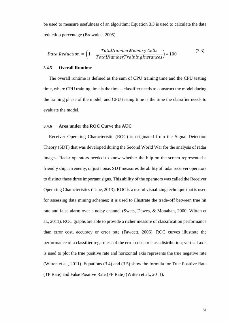
81
be used to measure usefulness of an algorithm; Equation 3.3 is used to calculate the data
reduction percentage (Brownlee, 2005).
𝐷𝑎𝑡𝑎 𝑅𝑒𝑑𝑢𝑐𝑡𝑖𝑜𝑛 = (1 −𝑇𝑜𝑡𝑎𝑙𝑁𝑢𝑚𝑏𝑒𝑟𝑀𝑒𝑚𝑜𝑟𝑦 𝐶𝑒𝑙𝑙𝑠
𝑇𝑜𝑡𝑎𝑙𝑁𝑢𝑚𝑏𝑒𝑟𝑇𝑟𝑎𝑖𝑛𝑖𝑛𝑔𝐼𝑛𝑠𝑡𝑎𝑛𝑐𝑒𝑠) ∗ 100
(3.3)
3.4.5 Overall Runtime
The overall runtime is defined as the sum of CPU training time and the CPU testing
time, where CPU training time is the time a classifier needs to construct the model during
the training phase of the model, and CPU testing time is the time the classifier needs to
evaluate the model.
3.4.6 Area under the ROC Curve the AUC
Receiver Operating Characteristic (ROC) is originated from the Signal Detection
Theory (SDT) that was developed during the Second World War for the analysis of radar
images. Radar operators needed to know whether the blip on the screen represented a
friendly ship, an enemy, or just noise. SDT measures the ability of radar receiver operators
to distinct these three important signs. This ability of the operators was called the Receiver
Operating Characteristics (Tape, 2013). ROC is a useful visualizing technique that is used
for assessing data mining schemes; it is used to illustrate the trade-off between true hit
rate and false alarm over a noisy channel (Swets, Dawes, & Monahan, 2000; Witten et
al., 2011). ROC graphs are able to provide a richer measure of classification performance
than error cost, accuracy or error rate (Fawcett, 2006). ROC curves illustrate the
performance of a classifier regardless of the error costs or class distribution; vertical axis
is used to plot the true positive rate and horizontal axis represents the true negative rate
(Witten et al., 2011). Equations (3.4) and (3.5) show the formula for True Positive Rate
(TP Rate) and False Positive Rate (FP Rate) (Witten et al., 2011):Rate

82
𝑇𝑃 𝑅𝑎𝑡𝑒 = 100 ∗ (𝑇𝑃
𝑇𝑃 + 𝐹𝑁)
(3.4)
3.1: False Positive Rate
𝐹𝑃 𝑅𝑎𝑡𝑒 = 100 ∗ (𝐹𝑃
𝐹𝑃 + 𝑇𝑁)
(3.5)
where TP is the number of true positives, FN is the number of false negatives, FP is the
number of false positives and TN is the number of true negatives. TP and TN are correct
classifications; FP is the number of outcomes when the prediction is positive when it is
actually negative, and FN is the number of outcomes when the prediction is negative
when it is actually positive (Witten et al., 2011).
The area under the curve (AUC) is a single quantity that summarizes ROC curves. This
area denotes the probability that a randomly selected positive instance is correctly ranked
with greater suspicion than a randomly chosen negative sample (Bradley, 1997). AUC is
the area under the ROC curve, the greater the area, the better the model (Witten et al.,
2011). A rough guide for classifying the accuracy of a test is the common academic
grading scale (Tape, 2013):
Excellent (A) = .90 to 1
Good (B) = .80 to .90
Fair (C) = .70 to .80
Poor (D) = .60 to .70
Fail (F) = .50 to .60
This means for example, if the area under ROC falls within [0.9, 1] the classifier
performs excellent and if it falls within [0.5, 0.6] it fails.
3.4.7 Student’s t test
It is common that the statistical significance between the mean of two results is tested
through student’s t-test (Jackson, 2012; Witten et al., 2011). When decisions are made,

83
making speculations or expectations about the populations involved are common. Such
expectations are called statistical hypotheses, which might or might not be true. There are
usually two types of hypotheses: a null hypothesis (Ho) which is tested against an
alternative hypothesis denoted by (H1). And two types of errors exist when we decide.
Type I error happens when we decide to reject a hypothesis although it should be
accepted, but when we accept a hypothesis although it should be rejected, then a Type II
error has occured. Both decision are wrong. The level of significance of the test is the
maximum probability with which we accept to make a Type I error. This probability is
usually represented by α. Although different values can be used for α, it is common to use
either .05 or .01. If for instance a .01 or 1% level of confidence is selected, then there is
1 percent the chance that we would reject the hypothesis when in fact it should be
accepted, in other words we are 99% confident that we have made the correct decision.
In such case we would be wrong with probability 1 which means that the hypothesis has
been rejected at 0.01 level of significance. α represents the level of significance, and the
level of confidence of the test is (1-α). Equations (3.6) and (3.7) present the null
hypothesis and its alternative hypothesis:
𝐻𝑜: 𝐴𝐼𝑅𝑆2𝑃𝑒𝑟𝑓𝑜𝑟𝑚𝑎𝑛𝑐𝑒 𝑚𝑒𝑎𝑛 = 𝑃𝑟𝑜𝑝𝑜𝑠𝑒𝑑 𝐴𝑙𝑔𝑜𝑟𝑖𝑡ℎ𝑚𝑝𝑒𝑟𝑓𝑜𝑟𝑚𝑎𝑐𝑒 𝑚𝑒𝑎𝑛 (3.6)
Hypsis
𝐻1: 𝐴𝐼𝑅𝑆2𝑃𝑒𝑟𝑓𝑜𝑟𝑚𝑎𝑛𝑐𝑒 𝑚𝑒𝑎𝑛 ≠ 𝑃𝑟𝑜𝑝𝑜𝑠𝑒𝑑 𝐴𝑙𝑔𝑜𝑟𝑖𝑡ℎ𝑚𝑝𝑒𝑟𝑓𝑜𝑟𝑚𝑎𝑐𝑒 𝑚𝑒𝑎𝑛 (3.7)
This thesis examines the hypothesis (Ho) that the mean values of two results are the
same. Throughout this thesis, we use the two-tailed t-test to decide if we can accept or
reject the null hypothesis. The p value will be determined and it is the likelihood that the
two means are equal. If p < α (this thesis uses α = .05), then we assume that this likelihood
is not sufficient for the difference between the means to be based just on chance, and
consequently we infer that there is a statistically significant difference in the means.
84
3.4.8 Classification Modelling
There are many classification models in the literature – from simple techniques such
as nearest neighbor and rule-based classifiers to more advanced techniques such as
ensemble methods and support vector machine (Pang-Ning Tan, 2006). This study uses
the support vector machine for classification modelling. The support vector machine is
introduced later in section 4.4.
3.5 Well-known classifiers
In order to evaluate the performance of the proposed algorithm, this thesis used various
well-known classifiers, these classifiers are used very often in business data mining and
they correspond to a variety of classifier types (Meng et al., 2005; Van der Putten, 2010)
as benchmark. These classifiers include AIRS2, 1-nearest neighbor (1-KNN), 7-nearest
neighbor 7-KNN , C4.5/J48 decision tree, CLONALG, Immunos99, LibSVM, Logistic,
multi-layer perceptron (MLP), Naïve Bayes, radial basis function network (RBF
Network), sequential minimal optimization with poly kernel (SMO), and sequential
minimal optimization with RBF kernel (SMO2). SMO is an implementation of John
Platt’s algorithm for training a support vector classifier.
In order to be consistent, all these classifiers were used under the same condition, and
all of them were available through the same environment, the WEKA where the proposed
algorithm was also implemented.
3.6 Summary
This chapter introduced theoretical background of the methodology that is used in this
thesis. We presented an overview of the current research and explained the experimental
setup including system specification, benchmark data sets, and parameter setup. Then we
introduced the performance metrics used in this thesis that is used to evaluate the
performance of classifiers. We concluded the chapter with introducing some well-known

85
classifiers that are used as benchmark to compare the performance obtained with the
proposed algorithm to the ones obtained with the well-known classifiers.
86
CHAPTER 4: IMPROVEMENT OF ARTIFICIAL IMMUNE RECOGNITION
SYSTEM 2
4.1 Introduction
This chapter introduces the methodology used to improve the performance of AIRS2.
Classification accuracy, running time, data reduction, and the area under ROC curve are
metrics that are discussed in this section.
Section 4.2 presents changes that were made to the resource allocation of the algorithm
and discusses fuzzy logic and its application for resource allocation. This section explains
the stages involved in building one of the proposed algorithm (the FRA-AIRS2).
Section 4.3 introduces real-world tournament selection mechanism and presents its
application in resource competition of the algorithm. This section explains the stages
involved in building one of the proposed algorithm (the RRC-AIRS2).
Section 4.4 introduces support vector machine, which will be used as the classifier of
the main proposed algorithm. This section explains the stages involved in building the
main proposed algorithm (the FSR-AIRS2). It explains how the previously developed and
discussed methods: FRA, RRC, and SVM are put together to build the FSR-AIRS2.
Section 4.5 introduces the experimental setup used to evaluate the performance of the
proposed classifier (the FSR-AIRS2).
Section 4.6 evaluates the behavior of proposed models: FRA-AIRS2, RRC-AIRS2,
and FSR-AIRS2 on benchmark data sets.
Section 4.6.1 evaluates and discusses performance of FRA-AIRS2. Section 4.6.1.1
compares classification accuracy obtained with FRA-AIRS2 and that of AIRS2 on
87
benchmark data sets. Section 4.6.1.2 compares running time obtained with FRA-AIRS2
and that of AIRS2 on benchmark data sets.
Section 4.6.2 evaluates and discusses performance of RRC-AIRS2. Section 4.6.2.1
compares classification accuracy obtained with RRC-AIRS2 and that of AIRS2 on
benchmark data sets. Section 4.6.2.2 compares running time obtained with RRC-AIRS2
and that of AIRS2 on benchmark data sets.
Section 4.6.3 evaluates and discusses performance of FSR-AIRS2. Section 4.6.3.1
evaluates and compares the classification accuracies obtained with AIRS2 and FSR-
AIRS2 on benchmark data sets. Section 4.6.3.2 compares the classification accuracies
obtained with the FSR-AIRS2 and other common classifiers. Section 4.6.3.3 discusses
the data reduction capabilities of AIRS2, FRA-AIRS2, and FSR-AIRS2.
Section 4.6.3.3(a) compares evolved memory cells through AIRS2 and FRA-AIRS2.
Section 4.6.3.3(b) compares data reduction capability of FSR-AIRS2 with that of AIRS2.
Section 4.6.3.4 discusses and compares the average running time obtained with FSR-
AIRS2 and other common classifiers
Section 4.6.3.5 discusses and compares the average area under the curve (AUC)
obtained with FSR-AIRS2 and other common classifiers.
4.2 Development of FRA-AIRS2
Following definitions (see Table 4.1) are taken from a document introduced by the
International Electrotechnical Commission (International-Electrothechnical-
Commission, 1997).
Fuzzy logic uses linguistic expressions to describe real numbers. Terms such as
“Low” or “Very High” are designated as linguistic terms and input variables that are

88
described by linguistic terms are known as linguistic values. Membership function is used
to describe the membership degree of each element in the universe of discourse.
Table 4.1: Definitions of Language Elements for Fuzzy Logic
Term Definition
Accumulation
(or result
aggregation)
Combinations of results of linguistic rules in a final result.
Aggregation Calculation of the degree of accomplishment of the condition of a
rule.
Activation The process by which the degree of fulfilment of a condition acts
on an output fuzzy set.
Crisp set A crisp set is a special case of a Fuzzy set, in which the
membership function only takes two values, commonly defined as 0
and 1.
Defuzzification Conversion of a Fuzzy set into a numerical value.
Degree of
membership
Membership function value.
Fuzzification Conversion of an input value into degrees of membership for the
membership functions defined on the variable taking this value.
Fuzzy Control A type of control in which the control algorithm is based on Fuzzy
Logic.
Inference Application of linguistic rules on input values in order to generate
output values
Linguistic rule IF-THEN rule with condition and conclusion, one or both at least
linguistic.
Linguistic term In the context of Fuzzy Control linguistic terms are defined by
Fuzzy sets.
Membership
function
A function which expresses in which degree an element of a set
belongs to a given Fuzzy subset.
Singleton A singleton is a Fuzzy set whose membership function is equal to
one at one point and equal to zero at all other points.
Rule base Collection of linguistic rules to attain certain objectives.
Figure 4.1 shows the structure and functional elements of Fuzzy Control.

89
Figure 4.1: Structure and Functional Elements of Fuzzy Control
Fuzzy control consists of processing measured values based on a collection of
linguistic rules which are also known as fuzzy rules. A Fuzzy Inference System (FIS)
maps input variables to output values, and fuzzy rules define how FIS should make a
decision about classifying an input or directing an output. The input variables are
measureable variables and the output variables are correcting real values. The process of
transferring input variables into degrees of membership values is called fuzzification; it
matches the input variables with the linguistic terms using a set of input membership
functions. A crisp output from a FIS represents the output and the process of transferring
output variables from fuzzy sets into real numbers is called defuzzification. Briefly, a FIS
calculates the output value as follows: first, it determines a set of fuzzy rules, then it
fuzzifies the inputs using the input membership functions, next it combines the just
fuzzified inputs based on the fuzzy rules in order to establish a rule strength, then it
combines the membership function and the rule strength in order to determine the
consequence of the rule. Further, FIS gets the output distribution by combining the
consequences, and finally it defuzzifies the output (International-Electrothechnical-
Commission, 1997).
There are many ways of defuzzification. The Center of Gravity (COG) method is used
in this thesis, because it is general and easy to compute. This method calculates the crisp
90
output by the sums of the center of gravities of the conclusions. Thus, a fuzzy inference
system can compute output y of an input vector x. The main purpose is to make the best
solution possible for each input vector. In the resource competition stage of AIRS, the
algorithms aim to improve the selection probability of high-affinity ARBs, for next steps.
Resource competition is subject to each ARB’s number of allocated resources, the
allocation depends on the similarity between the ARB and the antigen as well as its class.
Resource allocation for each ARB in AIRS2 is equal to the product of clonal rate and
stimulation value as it is presented in Equation (4.1): Originesource loc
ARB.res = clonalRate x ARB.stim 4.1:(4.1)
where ARB.res, clonalRate, ARB.stim are the number of allocated resources, a user
defined value, and stimulation value respectively. It means there is a linear relation
between the amount of allocated resource and the stimulation. As mentioned earlier,
researchers worked on solving similar linear issue in AIRS1, however this problem has
not been addressed in AIRS2 yet. AIRS2 also uses a linear resource allocation method,
and this linearity results in producing more memory cells which also causes longer
running time. This is because the difference between the number of high-affinity ARBs
and the number of low-affinity ARBs is low and this leads to allowing low-affinity ARBs
into the process of cloning and mutation which increases the number of memory cells and
prolongs the running time, one way to overcome the linearity issue and reduce the size of
data sets is to use fuzzy logic in order to prioritize the memory cells with higher affinity
over those with lower affinity therefore in this thesis the Equation (4.1) is replaced with
the Equation (4.2).
ARB.res = clonalRate × FuzzyStimulation (ARB.stim) (4.2)

91
where FuzzyStimulation function is a non-linear approach (see Figure 4.4) for regulating
the stimulation value. Figure 4.2 shows the process of fuzzy resource allocation of the
cloned MCmatch instances. Initially an instance “A” is presented to the memory cell pool,
“A” stimulates all memory cells in the pool and each cell in the pool is assigned a
stimulation value according to the Equation 2.2. This thesis uses the Euclidean distance
as the main metric for both affinity and stimulation; however, other distance metrics could
also be used. A vector with the greatest stimulation value is then selected as the best match
memory cell, and then the stimulation value of best match memory cell undergoes
fuzzification, before it is used in the process of affinity maturation.
Figure 4.2: Fuzzy Resource Allocation
Figure 4.3 illustrates the pseudocode for resource allocation method of FSR-AIRS2. It
is dubbed as Fuzzy Resource Allocation (FRA). This algorithm loops through all Cells in
the Cell Pool and allocates resources to the cells based on their fuzzy stimulation value.
In line 2 the algorithm calls FuzzyStimulation function (explained next) to get a fuzzy
value for the control parameter “stimulation” and multiplies this value in line 3 by the
92
ClonalRate to calculate the amount of resources. In line 4 the just calculated resource is
added to the total number of resources allocated for the Cell Pool. In line 6 the algorithm
orders the list of resources, so that the Cell with the highest stimulation is on the top of
the list. Line 7 returns the total amount of allocated resource.
Figure 4.3: Resource Allocation for RRC-AIRS2 and FSR-AIRS2
Figure 4.4 shows the steps for determining fuzzy value of the stimulation. The
algorithm uses Fuzzy Inference System (FIS), which is presented in line 1. In line 2 the
algorithm reads instructions for building the fuzzy model and employs fuzzy control
language for converting the variable ‘stimulation’ into degrees of membership for the
membership functions defined on this variable; the term ‘Fstimulation’ refers to the
output variable. The structure for fuzzy control language and its explanations follows (see
below for explanations about Figure 4.5). In line 3 the input variable “stimulation” is
defined, and line 4 uses the fuzzy instruction and input variable to evaluate the fuzzy
value. Line 5 returns the fuzzy value for the stimulation dubbed as Fstimulation. The
linguistic variable for ‘Fstimulation’ has to be defuzzified, i.e. converted into a value.
Input: CellPool; Output Resources
FuzzyResourceAllocation (CellPool) {
1 FOREACH Cell in CellPool DO {
2 fStim ← FuzzyStimulation (StimulatedResource) // get fuzzy stim
value
3 res ← fStim * ClonalRate // calculate resource allocation
4 resources ← resources + res
5 } ENDFOR
6 CellPool.orderByResources //order by allocated resources
7 return resource //output Resource
}

93
Input: Stimulation Value
Output: Fstimulation // Fuzzy Stimulation Value
FuzzyStimulation (Stimulation) {
1 FIS fis ← null
2 fis ← FIS.load (control file)
3 input ← Stimulation
4 Fstimulation = fis.evaluate()
5 return Fstimulation
}
Figure 4.4: Determine Fuzzy Value for Stimulation
Figure 4.5 illustrates elements of fuzzy control language that are used in resource
allocation procedure of FRA-AIRS2 and FSR-AIRS2. As can be seen the fuzzy control
language consists of a function block where the input and output variables are defined
(lines 1-8). The value of the input variable is converted into degrees of membership for
the membership function defined on this variable (lines 10-16). This thesis uses a
trapezoidal membership function, and it is defined by a set of points. Each point is
represented by a pair of values of the variable and the membership degree of that value.
Pairs are separated by commas. The linguistic variable “stimulation” is described by the
linguistic terms in order to fuzzify the variable (lines 11-15). The linguistic variable for
the output variable “Fstimulation” is converted into a value; this conversion is called
defuzzification (lines 18-29) In order to make the defuzzification easier, the singeltons,
(special membership functions) are used. The defuzzification method used in this study
is known as Center of Gravity for Singletons (COGS) (line 26), which is defined as:
𝑅𝑒𝑠𝑢𝑙𝑡 𝑜𝑓 𝑑𝑒𝑓𝑢𝑧𝑧𝑖𝑐𝑎𝑡𝑖𝑜𝑛 = ∑ 𝑟𝑖µ𝑖𝑛𝑖=1
∑ µ𝑖𝑛𝑖=1
(4.3)
where r is output variable, µ is membership function, and n is the number of singletons.
The Center of Gravity is a very common defuzzification method and is easy to use.
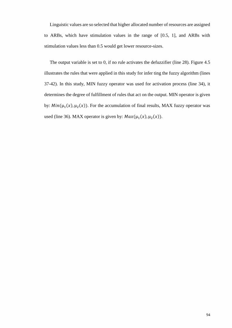
94
Linguistic values are so selected that higher allocated number of resources are assigned
to ARBs, which have stimulation values in the range of [0.5, 1], and ARBs with
stimulation values less than 0.5 would get lower resource-sizes.
The output variable is set to 0, if no rule activates the defuzzifier (line 28). Figure 4.5
illustrates the rules that were applied in this study for infer ting the fuzzy algorithm (lines
37-42). In this study, MIN fuzzy operator was used for activation process (line 34), it
determines the degree of fulfillment of rules that act on the output. MIN operator is given
by: 𝑀𝑖𝑛(µ1(𝑥), µ2(𝑥)). For the accumulation of final results, MAX fuzzy operator was
used (line 36). MAX operator is given by: 𝑀𝑎𝑥(µ1(𝑥), µ2(𝑥)).

95
FUNCTION_BLOCK Fuzzy_Command_File
1 // Input variable is defined here
2 VAR_INPUT
3 stimulation: REAL;
4 END_VAR
5 // Output variable is defined here
6 VAR_OUTPUT
7 Fstimulation: REAL;
8 END_VAR
9 // Fuzzify 'stimulation'
10 FUZZIFY stimulation
11 TERM VeryLow := (0, 1) (0.2, 0) ;
12 TERM Low := (0.1, 0) (0.2,1) (0.3,1) (0.4,0);
13 TERM Medium := (0.3, 0) (0.4,1) (0.5,1) (0.6,0);
14 TERM High := (0.5, 0) (0.6,1) (0.7,1) (0.8,0);
15 TERM VeryHigh := (0.7, 0) (0.8,1) (1,1);
16 END_FUZZIFY
17 // Defuzzify ‘Fstimulation’
18 DEFUZZIFY Fstimulation
19 TERM VeryLow := 0.1;
20 TERM Low := 0.35;
21 TERM Medium := 0.5;
22 TERM High := 0.75;
23 TERM VeryHigh := 1;
24 // Defuzzification method: 'Center Of Gravity Singleton'
26 METHOD : COGS;
27 // Default value: 0 (in case no rule activates defuzzifier)
28 DEFAULT := 0;
29 END_DEFUZZIFY
30 RULEBLOCK RB
31 // For ‘and’ use 'min'
32 AND: MIN;
33 // For activation method use 'min'
34 ACT: MIN;
35 // For accumulation method use 'max'
36 ACCU: MAX;
37 RULE 1: IF stimulation IS VeryLow THEN Fstimulation IS
VeryLow;
38 RULE 2: IF stimulation IS Low THEN Fstimulation IS Low;
39 RULE 3: IF stimulation IS Medium THEN Fstimulation IS Medium;
40 RULE 4: IF stimulation IS High THEN Fstimulation IS High;
41 RULE 5: IF stimulation IS VeryHigh
THEN Fstimulation IS VeryHigh;
42 END_RULEBLOCK
END_FUNCTION_BLOCK
Figure 4.5: Fuzzy Control Language for Resource Allocation of FRA-AIRS2
and FSRAIRS2
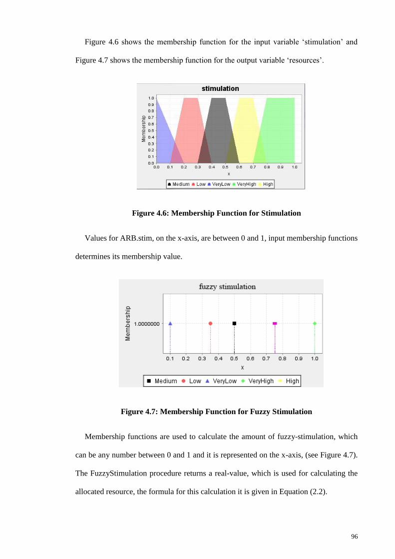
96
Figure 4.6 shows the membership function for the input variable ‘stimulation’ and
Figure 4.7 shows the membership function for the output variable ‘resources’.
Figure 4.6: Membership Function for Stimulation
Values for ARB.stim, on the x-axis, are between 0 and 1, input membership functions
determines its membership value.
Figure 4.7: Membership Function for Fuzzy Stimulation
Membership functions are used to calculate the amount of fuzzy-stimulation, which
can be any number between 0 and 1 and it is represented on the x-axis, (see Figure 4.7).
The FuzzyStimulation procedure returns a real-value, which is used for calculating the
allocated resource, the formula for this calculation it is given in Equation (2.2).

97
Evaluation of data reduction capabilities for both algorithms AIRS2 and FRA-AIRS2
are presented in subsection 4.6.3.3(a). There, we can see that for example, Liver Disorders
data set consists of 345 instances and while AIRS2 reduces the data set to approximately
197 records, FRA-AIRS2 reduces it to around 103 instances.
This thesis uses the FRA in step 5 of the 3rd stage of FSR-AIRS2 algorithm (explained
later in section 4.4.1) for refining resource allocation of ARBs.
4.3 Development of RRC-AIRS2
The difference between AIRS1 and AIRS2 is explained in detail in subsection 2.6.1.
As explained there, Watkins modified the procedures responsible for maintaining the
memory of system (resource management of AIRS2). AIRS1 used to generate clones of
multiple classes however only clones of the same class as the antigen are used in the ARB
pool (Brownlee, 2005), AIRS2 maintains only the ARBs of the same class and does not
allow mutation of the class value (switching classes are not permitted) this is in contrast
to how AIRS1 dealt with ARBs (Watkins, 2005).
While in AIRS1 a user has the ability to set the “mutate rate” parameter to control the
degree to mutate a created clone, AIRS2 uses the notion of somatic hypermutation where
the quantity of mutation of a produced clone is proportional to its affinity to the
concerning antigen (Brownlee, 2005). Nevertheless, the problem with linearity still exists,
and this issue has not been addressed in AIRS2 yet.
Tournament selection (TS) is one of useful, robust, and popular mechanism in genetic
algorithm. The selection pressure of ‘tournament selection’ varies directly as the
‘tournament size’ varies. Whenever the amount of competitors rise, the resulting selection
pressure rises too (Miller & Goldberg, 1995), and this leads to premature convergence
(Ahn, 2006). TS is considered to be effective in keeping the selection noise as low as

98
possible (Ahn, 2006). This study uses Real World Tournament Selection (RWTS) which
has shown good result in connection with AIRS1 in the work of (Golzari et al., 2009a,
2009b).
Lee et al. compared conventional TS and RWTS mechanism and discovered that the
later has a higher selection pressure with a higher sampling accuracy and relatively small
loss of diversity than the former. Authors concluded that RWTS preserves more diversity
than TS under similar selection pressure, and that sampling accuracy and higher pressure,
improve the performance in a selection strategy (Lee, Soak, Kim, Park, & Jeon, 2008).
Lee et al. also argued that excessive use of high pressure in a selection strategy is not
appropriate because it may cause a situation of premature convergence. Their results
showed that RWTS causes only a small loss of diversity and this is an indication that
RWTS does not have an excessive high selection pressure (Lee et al., 2008).
RWTS is widely used to find a winner in a sport game. The players or teams are
randomly grouped pair wise in sequence with a neighbor. If the number of players is an
odd number, the last individual will be paired with someone from the same tournament
level randomly, pairs compete and the winner of each pair goes to the next tournament
level. In the next round this procedure repeats by building new pairs and starting the
competition. At the end, one champion will be identified. The champion of the
tournament is the player with the best fitness value among all participating players. For
the resource competition, ARBs of each class represent individuals. ARBs enter the
competition and each ARB competes with a neighbor. This algorithm considers ARB A
as a neighbor of ARB B, if ARB B is the first ARB from the same class as ARB A, and
it is generated in the system after ARB A. The competition depends on the amount of
allocated resources for ARBs. This amount is calculated for each ARB during the
resource allocation process.

99
Figure 4.8 illustrates the pseudocode for RWTS-based Resource Competition method
which will be used by RRC-AIRS2 and FSR-AIRS2 models which will be explained in
sections 4.3.1 and section 4.4.1 respectively. This method is dubbed as RRC. In this
method each ARB has to compete with its neighbour.
Figure 4.8: Pseudocode for RWTS-Resource Competition (RRC)
RRC (ARBPool){
1 Resources Allowed ← Total Resources
2 Stimulate (ARBs.Stim)
3 Allocate resources to ARBs based on their Stimulation value
4 Allocated Resource ← Sum of allocated resources of ARBs
5 Current pair ← first pair of ARBs
6 //Continue until the resources are below a threshold
7 DOWHILE (Allocated Resource > Allowed Resource)
8 NumResToBeRemoved ← Allocated Resource – Resource Allowed
9 FOR Current pair
10 MinARB.resource ← ARB with the lower resource from the pair
11 //Check if element can be removed
12 IF MinARB.resource ≤ NumResToBeRemoved
13 Delete MinARB.resource from the population
14 Allocated Resource ← Allocated Resource –
MinARB.resource
15 ELSE
16 //Decrement resources
17 MinARB.resource ← MinARB.resource –
NumResToBeRemoved
18 Allocated Resource ← Allocated Resource –
NumResToBeRemoved
19 ENDIF
20 IF current pair is last ARB pair
21 GOTO first ARB pair
22 ELSE
23 GOTO next ARB pair
24 ENDIF
25 ENDFOR
26 ENDDOWHILE
27 //Compare Allocated Resources of ARBs
28 //The best ARB is always the one with the most resources
29 BestARB ← ARB with the most Allocated Resources
30 Return BestARB
}

100
As it can be seen from the Figure 4.8, in line 1 the algorithm determines the number
of allowed resources, which is set by the user, then ARBs are stimulated (line2) and
resources are allocated to ARBs, based on their fuzzy stimulation value (lines 3-4) and
then pairs of ARBs are built as described above and the first pair is selected (line 5), all
pairs undergo a competition (lines 9-25) and the process of competition for resources
continuous (lines 7-26) until the resources are below a threshold. In line 10 the algorithm
verifies which of the pair has lower resources allocated to it, the one with the lowest
resource will be removed from the population (line 13) and the winner will go to the next
level. The competition between remaining pairs continuous until allowed resources will
become either equal to the sum of allocated resources of remaining ARBs or equal to the
sum of allocated resources of all in the competition participating ARBs. If for all ARBs
that participate in the competition their sum of allocated resources is still higher than the
amount of allowed resources, the tournament goes to the next level. The same competition
rules exist across all levels of the tournament. The competition continuous until the sum
of allocated resources becomes equal or less than the amount of allowed resources. The
amount of allocated resources will be reduced by the amount of resources that was
allocated by the looser (line 14). In lines 16-18 the amount of resources will be decreased
and recalculated. The algorithm verifies whether or not other pairs exist (lines 20-24), if
exist, the process of competition between pairs repeats otherwise it goes to next level and
starts building new pairs with the winners of previous level and new competition starts.
At the end the strongest ARB (the one with the most resources) will survive (lines 27-
30).
The concept of RRC is illustrated in the following examples. Let us assume to have 10
ARBs and each ARB is denoted as 𝑥𝑖, where i = 1, 2,…,10. Each ARB has been allocated
resources as follows: 𝑥1 = 3, 𝑥2 = 6, 𝑥3 = 2, 𝑥4 = 4, 𝑥5 = 1, 𝑥6 = 10, 𝑥7 = 8, 𝑥8 =
5, 𝑥9 = 7, 𝑥10 = 9. Figure 4.9 illustrates the RRC process of the above mentioned

101
ARBs. Assuming that total allowed resources (TAR=37), total allocated resources (TA)
for all ARBs equals 55 (=1+2+3+...+9+10) which is greater than the TAR of 37, therefore
competition for resources start between neighbors as it is illustrated in the Figure 4.9, the
winner of each pair is the one with the highest resource allocated to it.
Figure 4.9: RRC One Level
For example the winner between 𝑥1 = 3 𝑎𝑛𝑑 𝑥2 = 6 is 𝑥2 = 6 which goes to the next
level (level 1), now TA = 55 – 3 = 52 which is still higher than TAR, and since we still
have other pairs of ARBs, the competition continues between 𝑥3 = 2 𝑎𝑛𝑑 𝑥4 = 4 where
the winner 𝑥4 = 4 goes to level 1, now TA = 52 – 2 = 50 which is still higher than
TAR=37, and the process of competition continues until all paired ARBs have competed
against each other and TA becomes 37 or less. Looking at ARBs at level 1, their sum of
allocated resource (TA = 37) is equal to TAR, and at this point the stop condition has
been reached and ARBs with 6, 4, 10, 8, and 9 resources are allowed to go through next
step of FSR-AIRS2 (step 6 of the pseudocode for FSR-AIRS2, that is explained later).
Figure 4.10 presents another example for RRC, here TAR is assumed to be 25. In order
to satisfy the stop condition, the competition continues from level 1 to level 2, and at the
end the ARBs with 6, 10, and 9 resources will be taken to the next step of FSR-AIRS2
(step 6 of pseudocode for FSR-AIRS2, that is explained later).
This thesis uses the RRC method, in step 5 of the 3rd stage of RRC-AIRS2 and FSR-
AIRS2 algorithms (explained in sections 4.3.1 and 4.4.1 respectively) in order to

102
determine and remove the weak cells during resource competition (it is a process for
population control of memory cell pool).
Figure 4.10: RRC Two Levels
Results of the evaluation of these algorithms are presented in sections 4.6.2.1
and 4.6.3.1.
4.3.1 Pseudocode for RRC-AIRS2
This section introduces a new algorithm. This model uses the RRC method that was
introduced above and implements it in the AIRS2, the resulting algorithm is dubbed as
the RRC-AIRS2. The goal of introducing this algorithm is to evaluate the application of
the RRC method and verify whether or not this method improves the performance of the
AIRS2.
Figure 4.11 illustrates the pseudocode for RRC-AIRS2 algorithm. Similar to the
AIRS2, (introduced in section 2.6), RRC-AIRS2 consists of four stages: in the first stage
data is normalized and initialized. In the second stage a memory cell is identified and
ARB is generated. In the third stage the algorithm deals with competition for resources,
here it uses the RRC method in the development process of a candidate memory cell. In
the fourth stage of the algorithm the potential candidate memory cell is introduced into
the set of already established memory cells.

103
In step 5 of the 3rd stage, RRC-AIRS2 uses RRC for determining and removing the
weak cells during resource competition (population control of memory cell pool).
In stage 4, the algorithm passes the memory cell pool M to the KNN for classification.
I. Initialize and normalize dataset
II. Seed the memory cell pool (M), if desired.
III. For each training example (antigen) do the following:
1. If M is empty, add antigen to M.
2. Select the memory cell (mc) in M of the same classification
having the highest affinity to antigen.
3. Clone mc in proportion to its affinity to antigen.
4. Mutate each clone and add to the B-cell pool (ARB).
5. Allocate resources to ARB
Use RRC (RWTS-mechanism) for removing the weak cells
(population control of ARB).
6. Calculate the average stimulation of ARB to antigen and
check for termination. If the termination condition is
satisfied, goto step 9.
7. Clone and mutate a random selection of B-cells in
ARB based upon their stimulation.
8. Loop back to step 5.
9. Select the B-cell in ARB with the highest affinity to
antigen (candidate). If candidate has a higher affinity to
antigen than mc add candidate to M. If mc and candidate are sufficiently
similar, then remove mc from M.
return M IV. Perform KNN classification using M.
Figure 4.11: Pseudocode for RRC-AIRS2
Evaluation of the model RRC-AIRS2 and its comparison with the AIRS2 is presented
in section 4.6.2.1. There, for instance, we can see from the Table 4.6 that the degree of
classification accuracy is statistically significantly increased from 88.24% (obtained with
the AIRS2) to 89.23% (obtained with the RRC-AIRS2) for the “Statlog (Image
Segmentation)” data set.
4.4 Development of FSR-AIRS2
Support vector machine (SVM) is originated from advanced statistical learning theory
(SVMS.org, 2010) it is recognised as a robust and state-of-the-art classification technique.
SVM is able to maximize the predictive accuracy of a model without overfitting the
104
training instances. SVM is mainly suitable for analyzing data with very large numbers of
predictor fields. SVM has found many applications in various disciplines, including bio
sequence analysis, bioinformatics, classification, concept extraction, customer
relationship management, character recognition, text mining, and speech and voice
recognition.
Vapnik et al. introduced SVM in 1995, and later the “soft margin” SVM was presented
by Cortes and Vapnik (Cortes & Vapnik, 1995).
SVM’s goal is to find an optimal hyperplanes in a multi-dimensional space, so that
different classes are separated. Through an iterative training algorithm, an ideal
hyperplane can be constructed. Cortes et al. have shown that constructing the optimal
hyperplane which separates a set of training data has to satisfy (Cortes & Vapnik, 1995):
�� = f(x,w,b) =𝑤𝑇.x + b = 0 (4.4)
where y is the predicted output, x is the input pattern, w is the weight vector, whereby w
is orthogonal to the hyperplane, and b is the bias. Values for w and b must be set during
the training process. Ideally no data points should fall into the margin, in this case the
optimal margin hyperplane coincide with constructed hyperplane (Cortes & Vapnik,
1995). In many cases, it is not possible to separate training data without error, in such
cases SVM allows a minimal number of errors, these errors are known as classification
errors. In other words, the goal is to determine the optimum balance between a maximum
margin and minimum classification error. To express this problem a slack variable is
introduced and now SVM tries to minimize the functional 4.5: ction
Φ(ξ) = ∑𝜉𝑖𝜎
𝑛
𝑖=1
(4.5)
for small 𝜎 > 0 , subject to the constraints

105
yi(wT. xi + b ) ≥ 1 − ξi
for all i = 1, …, n and ξi ≥ 0
(4.6)
If σ is small enough, the functional (4.5) represents the number of training errors. SVM
looks now for some minimal subset of training errors and attempts to exclude them from
the training set. The part of the dataset that is error-free can be separated without errors.
For separating the remaining part of the training data, SVM constructs an optimal
hyperplane by solving the following optimization problem for w and b (Cortes & Vapnik,
1995):
𝑚𝑖𝑛𝑤 1
2||𝑤||2 + C 𝐹(∑ 𝜉𝑖
𝜎𝑛𝑖=1 ) (4.7)
subject to:
𝑦𝑖(𝑤𝑇 . 𝑥𝑖 + b ) ≥ 1 − 𝜉𝑖,
ξi ≥ 0,
for all i = 1, …, n
for all i = 1, …, n (4.8)
where C is a user defined constant, also known as the tuning parameter, it weights in-
sample classification errors and therefore controls the generalization ability of an SVM.
C controls the trade-off between the frequency of the error and complexity of the decision
rule (Cortes & Vapnik, 1995). If C increases, the classification accuracy for the training
data improves too; however this may cause overfitting. Cortes et al. demonstrated that
for solving this optimization problem, the saddle point of Lagrangian function can be
used. This function has to be minimized with respect to w, b, and , and maximized with
respect to Lagrange multipliers ∝ (Cortes & Vapnik, 1995).Function
L(w,b,∝) = 𝑚𝑖𝑛𝑤,𝑏𝑚𝑎𝑥∝{1
2||𝑤||
2− ∑ ∝𝑖
𝑛𝑖=1 [𝑦𝑖(𝑤. 𝑥𝑖 + 𝑏) − 1]} (4.9)

106
This is a classical optimization problem. To solve this problem, standard Quadratic
Programming (QP) techniques are used. It should be noted that only a few training
vectors𝑥𝑖 with ∝i greater than zero have an effective contribution to the sum (4.9) (Cortes
& Vapnik, 1995). Cortes et al. used Kuhn-Tucker theorem and showed that the
corresponding 𝑥𝑖 lie on the margin and satisfy (Cortes & Vapnik, 1995):
𝑦𝑖(𝑤. 𝑥𝑖 + 𝑏) = 1 (4.10)
These points (𝑥𝑖), whose ∝i ≠ 0, are called support vectors (SV). They are relevant
for the calculation of w, and the hyperplane is determined by SV. SVs lie either on the
margin boundaries or, for non-perfectly separable data, within the margin. The
complexity of calculations does not depend on the dimension of the input space but on
the number of support vectors, which is a minor subdivision of the training vector (Laura
Auria, 2008).
The decision or classification function 𝑔(𝑥) can be written as follows:
𝑔(𝑥) = 𝑠𝑖𝑔𝑛(∑ ∝𝑖𝑛𝑖=1 𝑦𝑖𝐾(𝑥𝑖, 𝑥𝑗) + 𝑏) (4.11)
where 𝐾(𝑥𝑖 , 𝑥𝑗) is the value of a kernel function satisfying the Mercer theorem. Functions
that satisfy Mercer’s theorem ensure that inner (dot) products can be used as kernels
(Laura Auria, 2008). SVM models can use a number of Kernels, including linear,
polynomial, sigmoid, and radial basis function (RBF) (Statsoft, 2013):
Kernel Functions:
𝐾(𝑥𝑖, 𝑥𝑗)
=
{
𝑥𝑖𝑥𝑖
(𝛾𝑥𝑖 𝑥𝑗 + 𝑐𝑜𝑒𝑓𝑓𝑖𝑐𝑖𝑒𝑛𝑡)𝑑
exp (−𝛾 |𝑥𝑖 − 𝑥𝑗|2)
tanh(𝛾𝑥𝑖 𝑥𝑗 + 𝑐𝑜𝑒𝑓𝑓𝑖𝑐𝑖𝑒𝑛𝑡)
𝐿𝑖𝑛𝑒𝑎𝑟
𝑃𝑜𝑙𝑦𝑛𝑜𝑚𝑖𝑎𝑙
𝑅𝑎𝑑𝑖𝑎𝑙 𝐵𝑎𝑠𝑖𝑠 𝐹𝑢𝑛𝑐𝑡𝑖𝑜𝑛 (𝑅𝐵𝐹)
𝑆𝑖𝑔𝑚𝑜𝑖𝑑
(4.12)

107
where is a kernel parameter. If the value of increases, the classification accuracy
improves, however this may cause overfitting too.
4.4.1 Pseudocode of FSR-AIRS2
This section introduces a new artificial immune system based hybrid algorithm. This
model uses the FRA, RRC, and SVM methods that were introduced in sections 4.2,
and 4.3, and implements them in the AIRS2; the resulting algorithm is dubbed as the FSR-
AIRS2. Figure 4.12 illustrates the pseudocode for FSR-AIRS2 algorithm that is used in
this study.
I. Initialize and normalize dataset
II. Seed the memory cell pool (M), if desired.
III. For each training example (antigen) do the following:
1. If M is empty, add antigen to M.
2. Select the memory cell (mc) in M of the same classification
having the highest affinity to antigen.
3. Clone mc in proportion to its affinity to antigen.
4. Mutate each clone and add to the B-cell pool (ARB).
5. Use FRA (Fuzzy-logic) to allocate resources to ARB
Use RRC (RWTS-mechanism) for removing the weak cells
(population control of ARB).
6. Calculate the average stimulation of ARB to antigen and
check for termination. If the termination condition is
satisfied, goto step 9.
7. Clone and mutate a random selection of B-cells in
ARB based upon their stimulation.
8. Loop back to step 5.
9. Select the B-cell in ARB with the highest affinity to
antigen (candidate). If candidate has a higher affinity to
antigen than mc add candidate to M. If mc and candidate are sufficiently
similar, then remove mc from M.
return M //prepare content of M for SVM
IV. Transfer M to SVM format
//run SVM as classifier
V. Perform SVM classification using M.
Figure 4.12: Pseudocode for FSR-AIRS2
108
Similar to AIRS2, (introduced in section 2.5), there are five stages in FSR-AIRS2: the
first stage consists of data normalization and initialization; also in this stage, optionally
memory cell pool can be seeded. The second stage is where, a memory cell is identified
and ARB is generated. The third stage handles competition for resources, and the
development process for a candidate memory cell happens here. In the fourth stage of the
algorithm, the potential candidate memory cell is introduced into the set of already
established memory cells. In step 5 of the 3rd stage, FSR-AIRS2 uses FRA (explained
in section 4.2) to refine resource allocation for ARBs and then it uses RRC (explained in
section 4.3) for determining and removing the weak cells during resource competition
(population control of memory cell pool).
In stage 4, the proposed algorithm formats the content of M so that it is prepared for
the SVM. In the stage 5, this algorithm passes M to the SVM for classification.
This research used WLSVM (EL-Manzalawy & Honavar, 2005) which is a wrapper
of LibSVM (Chang & Lin, 2011) inside WEKA (Mark Hall et al., 2009) to address
classification problems. The LibSVM supports multi-class classification and both “one-
against-one” and “one-against-the rest” multi-class strategies are part of the
implementation.
4.5 Experimental Setup
The goal of the experiment is to evaluate the performance of FSR-AIRS2 in a real-
world application setting. Details about data sets, performance and evaluation
measurements were discussed in Chapter 3.
Performance of other developed algorithms the FRA-AIRS2 and RRC-AIRS2 are also
evaluated.

109
4.6 Results and Discussion
This section evaluates the behaviour of the current implementation of the FRA-AIRS2,
RRC-AIRS2, and FSR-AIRS2 on some machine learning data sets. The standard machine
learning data sets employed in this section have been used to investigate the performance
of many different classification systems. This section compares the accuracy of the
current implementation with the accuracy of other classifiers using the mentioned data
sets. Table 4.2 presents the optimized parameter settings used to run AIRS2, FRA-AIRS2,
and RRC-AIRS2 on the standard machine learning data sets as well as the classification
accuracy obtained with AIRS2; the standard deviations are shown in parenthesis. The
parameters that were used include Affinity Threshold Scalar (ATS), Clonal Rate (CR),
Hypermutation Rate (HR), K-value for KNN classifier, Seed cells (S), Stimulation Value
(St), and number of Resources (NR).
Table 4.2: Parameter Settings used for AIRS2, FRA-AIRS2, and RRC-AIRS2.
Training Set ATS CR HR K S St NR
Balance Scale 0.2 10 0.5 10 1 0.9 150
Breast Cancer Wisconsin
(Diagnostic)
0.2 10 6.0 3 1 0.9 150
Contact Lenses 0.1 10 2.7 4 1 0.9 150
Ionosphere 0.2 10 2.0 3 1 0.9 350
Iris 0.2 10 2.0 3 1 0.9 150
Liver Disorders 0.2 10 2.0 3 1 0.9 150
Lung Cancer 0.2 10 0.2 4 1 0.9 150
Pima Indians 0.2 10 1.4 15 1 0.9 150
Statlog (Heart) 0.2 10 0.2 5 1 0.9 150
Statlog (Image Segmentation) 0.2 10 2.0 2 1 0.9 150
Statlog (Vehicle Silhouettes) 0.2 10 2.9 4 1 0.9 150
Sonar, Mines vs. Rocks 0.2 10 2.0 2 1 0.9 150
Vertebral Column_2C 0.2 10 2.0 3 1 0.9 150
Vertebral Column_3C 0.2 10 2.0 3 1 0.9 150
Wisconsin Breast Cancer Data
Set (WBCD) (Original)
0.2 10 3 5 2 0.9 200
Similar to the work of (Hamaker & Boggess, 2004) we did the following to determine
the parameters for AIRS2.
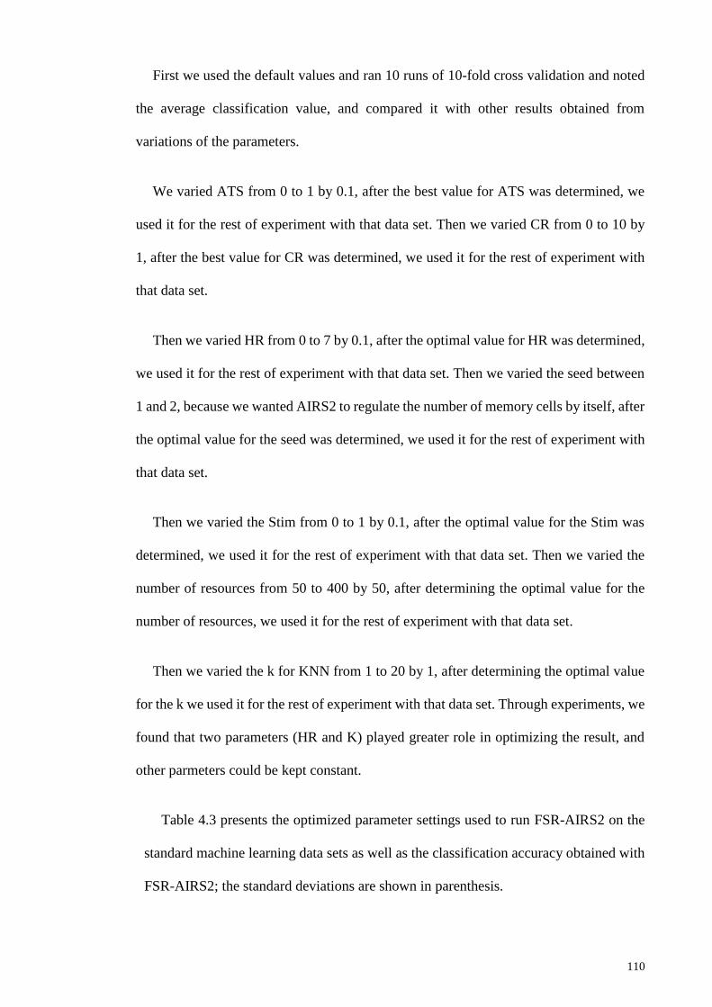
110
First we used the default values and ran 10 runs of 10-fold cross validation and noted
the average classification value, and compared it with other results obtained from
variations of the parameters.
We varied ATS from 0 to 1 by 0.1, after the best value for ATS was determined, we
used it for the rest of experiment with that data set. Then we varied CR from 0 to 10 by
1, after the best value for CR was determined, we used it for the rest of experiment with
that data set.
Then we varied HR from 0 to 7 by 0.1, after the optimal value for HR was determined,
we used it for the rest of experiment with that data set. Then we varied the seed between
1 and 2, because we wanted AIRS2 to regulate the number of memory cells by itself, after
the optimal value for the seed was determined, we used it for the rest of experiment with
that data set.
Then we varied the Stim from 0 to 1 by 0.1, after the optimal value for the Stim was
determined, we used it for the rest of experiment with that data set. Then we varied the
number of resources from 50 to 400 by 50, after determining the optimal value for the
number of resources, we used it for the rest of experiment with that data set.
Then we varied the k for KNN from 1 to 20 by 1, after determining the optimal value
for the k we used it for the rest of experiment with that data set. Through experiments, we
found that two parameters (HR and K) played greater role in optimizing the result, and
other parmeters could be kept constant.
Table 4.3 presents the optimized parameter settings used to run FSR-AIRS2 on the
standard machine learning data sets as well as the classification accuracy obtained with
FSR-AIRS2; the standard deviations are shown in parenthesis.
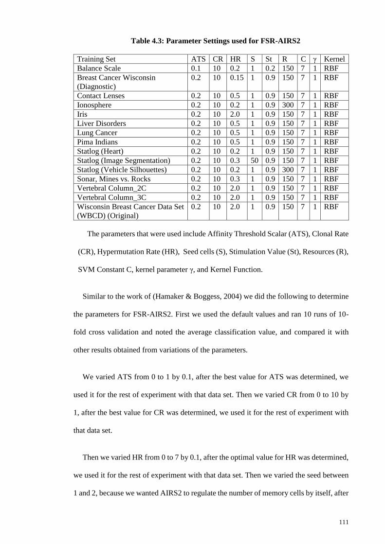
111
Table 4.3: Parameter Settings used for FSR-AIRS2
Training Set ATS CR HR S St R C γ Kernel
Balance Scale 0.1 10 0.2 1 0.2 150 7 1 RBF
Breast Cancer Wisconsin
(Diagnostic)
0.2 10 0.15 1 0.9 150 7 1 RBF
Contact Lenses 0.2 10 0.5 1 0.9 150 7 1 RBF
Ionosphere 0.2 10 0.2 1 0.9 300 7 1 RBF
Iris 0.2 10 2.0 1 0.9 150 7 1 RBF
Liver Disorders 0.2 10 0.5 1 0.9 150 7 1 RBF
Lung Cancer 0.2 10 0.5 1 0.9 150 7 1 RBF
Pima Indians 0.2 10 0.5 1 0.9 150 7 1 RBF
Statlog (Heart) 0.2 10 0.2 1 0.9 150 7 1 RBF
Statlog (Image Segmentation) 0.2 10 0.3 50 0.9 150 7 1 RBF
Statlog (Vehicle Silhouettes) 0.2 10 0.2 1 0.9 300 7 1 RBF
Sonar, Mines vs. Rocks 0.2 10 0.3 1 0.9 150 7 1 RBF
Vertebral Column_2C 0.2 10 2.0 1 0.9 150 7 1 RBF
Vertebral Column_3C 0.2 10 2.0 1 0.9 150 7 1 RBF
Wisconsin Breast Cancer Data Set
(WBCD) (Original)
0.2 10 2.0 1 0.9 150 7 1 RBF
The parameters that were used include Affinity Threshold Scalar (ATS), Clonal Rate
(CR), Hypermutation Rate (HR), Seed cells (S), Stimulation Value (St), Resources (R),
SVM Constant C, kernel parameter γ, and Kernel Function.
Similar to the work of (Hamaker & Boggess, 2004) we did the following to determine
the parameters for FSR-AIRS2. First we used the default values and ran 10 runs of 10-
fold cross validation and noted the average classification value, and compared it with
other results obtained from variations of the parameters.
We varied ATS from 0 to 1 by 0.1, after the best value for ATS was determined, we
used it for the rest of experiment with that data set. Then we varied CR from 0 to 10 by
1, after the best value for CR was determined, we used it for the rest of experiment with
that data set.
Then we varied HR from 0 to 7 by 0.1, after the optimal value for HR was determined,
we used it for the rest of experiment with that data set. Then we varied the seed between
1 and 2, because we wanted AIRS2 to regulate the number of memory cells by itself, after

112
the optimal value for the seed was determined, we used it for the rest of experiment with
that data set. Then we varied the Stim from 0 to 1 by 0.1, after the optimal value for the
Stim was determined, we used it for the rest of experiment with that data set. Then we
varied the number of resources from 50 to 400 by 50, after determining the optimal value
for the number of resources, we used it for the rest of experiment with that data set. One
exception was in case of the Statlog (Image Segmentation) data set, where we found seed
=50 as optimal value. For the SVM, we used RBF as the kernel function, as it is a
reasonable choice for linear and non-linear problems, and most importantly, it has only
two parameters to be set (C and γ) (Hsu, Chang, & Lin, 2003). This study used the default
values C = 7, γ = 1, which were given in LibSVM (Chang & Lin, 2011; EL-Manzalawy
& Honavar, 2005).
4.6.1 Evaluation of FRA-AIRS2
This section compares the results obtained from AIRS (AIRS2) and the FRA-AIRS2.
Since AIRS2 has been a successful classifier, it is important to verify whether or not the
changes to the algorithm have improved the classification accuracy.
4.6.1.1 Classification Accuracy of FRA-AIRS2 versus AIRS2
Table 4.4 shows the best average test set accuracies, together with the standard
deviations (given in parenthesis), obtained from AIRS2 and FRA-AIRS2 on the
benchmark data sets and p-value results of the student t-test comparing the mean
accuracies for AIRS2 and FRA-AIRS2.
All experiments utilized 10 fold cross validation and were averaged over 10 runs. The
Student’s t-test, as described in section 3.4.7, is used for testing the statistical significance
between the mean of the two results.

113
Table 4.4: Comparative Average Accuracies FRA-AIRS2 versus AIRS2
Training Set AIRS2 (STD) FRA-AIRS2
(STD)
p-value
Balance Scale 86.83% (3.14) 90.54% (2.49) p < 0.05
Breast Cancer Wisconsin
(Diagnostic)
96.17% (2.32) 98.08% (1.16) p < 0.05
Contact Lenses 82.83% (22.53) 83.00% (15.81) 0.92
Ionosphere 86.04% (4.84) 93.02% (2.41) p < 0.05
Iris 94.67% (5.36) 96.33% (4.26) 0.89
Liver Disorders 59.80% (8.18) 69.48% (6.3) p < 0.05
Lung Cancer 41.83% (26.64) 49.50% (25.90) p < 0.05
Pima Indians 74.41% (5.11) 86.97% (2.62) p < 0.05
Statlog (Heart) 77.48% (8.42) 80.96% (6.48) p < 0.05
Statlog (Image Segmentation) 88.24% (2.35) 89.65% (4.98) p < 0.05
Statlog (Vehicle Silhouettes) 62.56% (4.64) 71.18% (4.72) p < 0.05
Sonar, Mines vs. Rocks 65.60% (10.48) 72.46% (8.97) p < 0.05
Vertebral Column_2C 76.23% (8.70) 82.79% (5.33) p < 0.05
Vertebral Column_3C 72.84% (8.32) 80.01% (5.26) p < 0.05
Wisconsin Breast Cancer Data
Set (WBCD) (Original)
96.58% (2.19) 98.29% (1.09) p < 0.05
Table 4.4 shows that the changes made to the AIRS2 algorithm have improved the
classification accuracy. Results show that the differences in accuracy for almost all
benchmark are significant at the 95% significant level (α = 0.05) based on a two-tailed
student’s t-test as described in section 3.4.7.
When we compare the mean classification accuracy for the Balance Scale data set
obtained with the AIRS2 (𝑛1 =100, M=86.83%, SD=3.14) to the one obtained with FRA-
AIRS2 (𝑛2 =100, M=90.54%, SD=2.49) p<.05 the results show that the differences are
statistically significant at the 95% significant level (α = 0.05) for this data set. The FRA-
AIRS2 achieved significantly higher classification accuracy.
Comparing the mean classification accuracy for the Breast Cancer Wisconsin
(Diagnostic) data set obtained with AIRS2 (𝑛1 =100, M=96.17%, SD=2.32) to the one
obtained with the FRA-AIRS2 (𝑛2 =100, M=98.08%, SD=1.16) p<.05 the results show
that the differences are statistically significant at the 95% significant level (α = 0.05) for
this data set and the FRA-AIRS2 achieved significantly higher classification accuracy.

114
In the case of Contact Lenses data set, the comparison of the mean classification
accuracy obtained with the AIRS2 (𝑛1 =100, M=82.83%, SD=22.53) to the one obtained
with the FRA-AIRS2 (𝑛2 =100, M=83.0%, SD=15.81) p=.92 shows that the differences
are statistically insignificant at the 95% significant level (α = 0.05) for this data set.
When we compare the mean classification accuracy for the Ionosphere data set
obtained with the AIRS2 (𝑛1 =100, M=86.04%, SD=4.84) to the one obtained with the
FRA-AIRS2 (𝑛2 =100, M=93.02%, SD=2.41) p<.05 the results show that the differences
are statistically significant at the 95% significant level (α = 0.05) for this data set and the
FRA-AIRS2 achieved significantly higher classification accuracy.
Comparing the mean classification accuracy for the Iris data set obtained with the
AIRS2 (𝑛1 =100, M=94.67%, SD=5.36) to the one obtained with the FRA-AIRS2
(𝑛2 =100, M=96.33%, SD=4.26) p<.05 the results show that the differences are
statistically insignificant at the 95% significant level (α = 0.05) for this data set. However,
the FRA-AIRS2 achieved slightly higher classification accuracy.
In the case of Liver Disorders data set, the comparison of the mean classification
accuracy obtained with the AIRS2 (𝑛1 =100, M=59.8%, SD=8.18) to the one obtained
with the FRA-AIRS2 (𝑛2 =100, M=69.48%, SD=6.3) p<.05 the results show that the
differences are statistically significant at the 95% significant level (α = 0.05) for this data
set and the FRA-AIRS2 achieved significantly higher classification accuracy.
When we compare the mean classification accuracy for the Lung Cancer data set
obtained with the AIRS2 (𝑛1 =100, M=41.83%, SD=26.64) to the one obtained with FRA-
AIRS2 (𝑛2 =100, M=49.5%, SD=25.9) p<.05 the results show that the differences are
statistically significant at the 95% significant level (α = 0.05) for this data set and the
FRA-AIRS2 achieved significantly higher classification accuracy.
115
Comparing the mean classification accuracy for the Pima Indians data set obtained
with AIRS2 (𝑛1 =100, M=74.41%, SD=5.11) to the one obtained with FRA-AIRS2
(𝑛2 =100, M=86.97%, SD=2.62) p<.05 the results show that the differences are
statistically significant at the 95% significant level (α = 0.05) for this data set and the
FRA-AIRS2 achieved significantly higher classification accuracy.
In the case of Statlog (Heart) data set, the comparison of the mean classification
accuracy obtained with the AIRS2 (𝑛1 =100, M=77.48%, SD=8.42) to the one obtained
with the FRA-AIRS2 (𝑛2 =100, M=80.96%, SD=6.48) p<.05 the results show that the
differences are statistically significant at the 95% significant level (α = 0.05) for this data
set and the FRA-AIRS2 achieved significantly higher classification accuracy.
When we compare the mean classification accuracy for the Statlog (Image
Segmentation) data set obtained with the AIRS2 (𝑛1 =100, M=88.24%, SD=2.35) to the
one obtained with the FRA-AIRS2 (𝑛2 =100, M=89.65%, SD=4.98) p<.05 the results
show that the differences are statistically significant at the 95% significant level (α = 0.05)
for this data set and the FRA-AIRS2 achieved significantly higher classification accuracy.
Comparing the mean classification accuracy for the Statlog (Vehicle Silhouettes) data
set obtained with AIRS2 (𝑛1 =100, M=62.56%, SD=4.64) to the one obtained with the
FSR-AIRS2 (𝑛2 =100, M=71.18%, SD=4.72) p<.05 the results show that the differences
are statistically significant at the 95% significant level (α = 0.05) for this data set and the
FRA-AIRS2 achieved significantly higher classification accuracy.
In the case of Sonar, Mines vs. Rocks data set, the comparison of the mean
classification accuracy obtained with the AIRS2 (𝑛1 =100, M=65.6%, SD=10.48) to the
one obtained with the FRA-AIRS2 (𝑛2 =100, M=72.46%, SD=4.55) p<.05 the results
116
show that the differences are statistically significant at the 95% significant level (α = 0.05)
for this data set and the FRA-AIRS2 achieved significantly higher classification accuracy.
When we compare the mean classification accuracy for the Vertebral Column_2C data
set obtained with the AIRS2 (𝑛1 =100, M=76.23%, SD=8.7) to the one obtained with the
FRA-AIRS2 (𝑛2 =100, M=82.79%, SD=5.33) p<.05 the results show that the differences
are statistically significant at the 95% significant level (α = 0.05) for this data set and the
FRA-AIRS2 achieved significantly higher classification accuracy.
Comparing the mean classification accuracy for the Vertebral Column_3C data set
obtained with AIRS2 (𝑛1 =100, M=72.84%, SD=8.32) to the one obtained with the FSR-
AIRS2 (𝑛2 =100, M=80.01%, SD=5.26) p<.05 the results show that the differences are
statistically significant at the 95% significant level (α = 0.05) for this data set and the
FRA-AIRS2 achieved significantly higher classification accuracy.
In the case of Wisconsin Breast Cancer Data Set (WBCD) (Original) data set, the
comparison of the mean classification accuracy obtained with the AIRS2 (𝑛1 =100,
M=96.58%, SD=2.19) to the one obtained with the FRA-AIRS2 (𝑛2 =100, M=98.29%,
SD=1.09) p<.05 the results show that the differences are statistically significant at the
95% significant level (α = 0.05) for this data set and the FRA-AIRS2 achieved
significantly higher classification accuracy.
In general, since α ≥ p on almost all benchmark data sets, it can be concluded that
modifications introduced in FRA-AIRS2 appear to have positive effect on the
classification accuracy of the classifier. The comparison with AIRS2 shows that FRA-
AIRS2 has statistically significantly increased the classification accuracy on almost all
(13 out of 15) benchmark data sets.

117
Figure 4.13 illustrates a graphical comparison of classification accuracy on benchmark
data sets obtained with AIRS2 and FRA-AIRS2 algorithms.
Figure 4.13: Comparison of Classification Accuracy AIRS2 versus FRA-AIRS2 on
benchmark data sets
Figure 4.13 shows that FRA-AIRS2 has achieved higher classification accuracy than
AIRS2 on 13 out of 15 benchmark data sets.
4.6.1.2 Comparing Running Time of FRA-AIRS2 and AIRS2 on benchmark data
sets
This section compares the running time results obtained from AIRS2 and the FRA-
AIRS2. Since AIRS2 has been a successful classifier, it is important to verify whether or
not the changes to the algorithm have improved the running time. Table 4.5 shows the
best average test set running time, together with the standard deviations (given in
parenthesis), obtained from AIRS2 and FRA-AIRS2 on the benchmark data sets and p-
0.0010.0020.0030.0040.0050.0060.0070.0080.0090.00
100.00
Balan
ce Scale
Breast C
ancer W
iscon
sin(D
iagno
stic)
Co
ntact Le
nse
s
Ion
osp
here
Iris
Liver Diso
rders
Lun
g Can
cer
Pim
a Ind
ians
Statlog (H
eart)
Statlog (Im
ageSe
gmen
tation
)
Statlog (V
ehicle Silh
ou
ettes)
Son
ar, Min
es vs. Ro
cks
Verte
bral C
olu
mn
_2C
Verte
bral C
olu
mn
_3C
Wisco
nsin
Breast C
ancer
Data Set (W
BC
D) (O
riginal)
Acc
ura
cy
Data sets
AIRS2 FRA-AIRS2
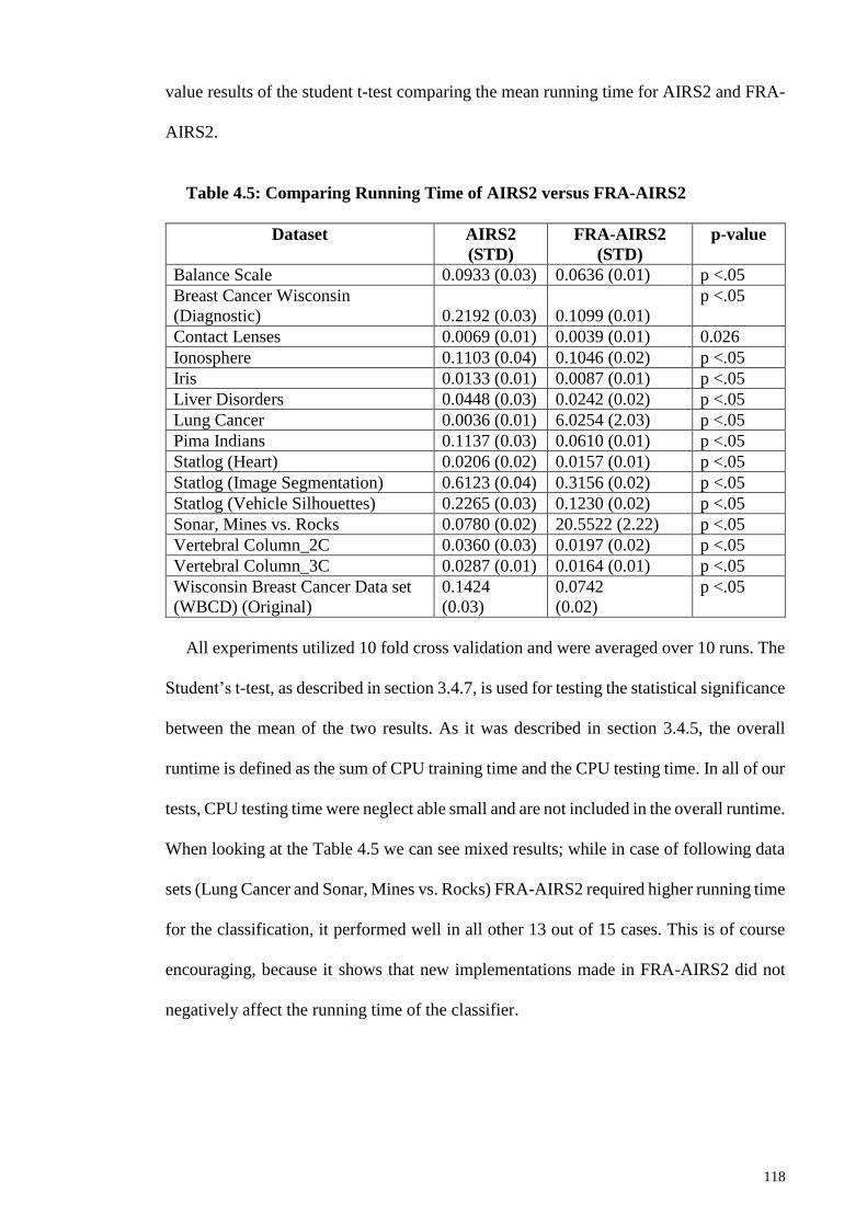
118
value results of the student t-test comparing the mean running time for AIRS2 and FRA-
AIRS2.
Table 4.5: Comparing Running Time of AIRS2 versus FRA-AIRS2
Dataset AIRS2
(STD)
FRA-AIRS2
(STD)
p-value
Balance Scale 0.0933 (0.03) 0.0636 (0.01) p <.05
Breast Cancer Wisconsin
(Diagnostic) 0.2192 (0.03) 0.1099 (0.01)
p <.05
Contact Lenses 0.0069 (0.01) 0.0039 (0.01) 0.026
Ionosphere 0.1103 (0.04) 0.1046 (0.02) p <.05
Iris 0.0133 (0.01) 0.0087 (0.01) p <.05
Liver Disorders 0.0448 (0.03) 0.0242 (0.02) p <.05
Lung Cancer 0.0036 (0.01) 6.0254 (2.03) p <.05
Pima Indians 0.1137 (0.03) 0.0610 (0.01) p <.05
Statlog (Heart) 0.0206 (0.02) 0.0157 (0.01) p <.05
Statlog (Image Segmentation) 0.6123 (0.04) 0.3156 (0.02) p <.05
Statlog (Vehicle Silhouettes) 0.2265 (0.03) 0.1230 (0.02) p <.05
Sonar, Mines vs. Rocks 0.0780 (0.02) 20.5522 (2.22) p <.05
Vertebral Column_2C 0.0360 (0.03) 0.0197 (0.02) p <.05
Vertebral Column_3C 0.0287 (0.01) 0.0164 (0.01) p <.05
Wisconsin Breast Cancer Data set
(WBCD) (Original)
0.1424
(0.03)
0.0742
(0.02)
p <.05
All experiments utilized 10 fold cross validation and were averaged over 10 runs. The
Student’s t-test, as described in section 3.4.7, is used for testing the statistical significance
between the mean of the two results. As it was described in section 3.4.5, the overall
runtime is defined as the sum of CPU training time and the CPU testing time. In all of our
tests, CPU testing time were neglect able small and are not included in the overall runtime.
When looking at the Table 4.5 we can see mixed results; while in case of following data
sets (Lung Cancer and Sonar, Mines vs. Rocks) FRA-AIRS2 required higher running time
for the classification, it performed well in all other 13 out of 15 cases. This is of course
encouraging, because it shows that new implementations made in FRA-AIRS2 did not
negatively affect the running time of the classifier.

119
4.6.2 Evaluation of RRC-AIRS2
This section compares the results obtained from AIRS2 and the proposed RRC-AIRS2.
Since AIRS2 has been a successful classifier, it is important to verify whether or not the
changes to the algorithm have improved the classification accuracy.
4.6.2.1 Classification Accuracy of RRC-AIRS2 versus AIRS2
Table 4.6 shows the best average test set accuracies, together with the standard
deviations (given in parenthesis), obtained from AIRS2 and RRC-AIRS2 on the
benchmark data sets and p-value results of the student t-test comparing the mean
accuracies for AIRS2 and RRC-AIRS2. All experiments utilized 10 fold cross validation
and were averaged over 10 runs. The Student’s t-test, as described in section 3.4.7, is used
for testing the statistical significance between the mean of the two results. Table 4.6
shows that the changes made to the AIRS2 algorithm have improved the classification
accuracy. Results show that the differences in accuracy for some benchmark are
significant at the 95% significant level (α = 0.05) based on a two-tailed student’s t-test.
Table 4.6: Comparative Average Accuracies AIRS2 versus RRC-AIRS2
Training Set AIRS2 (STD) RRC-AIRS2
(STD)
p-value
Balance Scale 86.83% (3.14) 86.9% (2.81) 0.74
Breast Cancer Wisconsin
(Diagnostic)
96.17% (2.32) 96.82% (2.24) 0.94
Contact Lenses 82.83% (22.53) 82.17% (22.88) 0.47
Ionosphere 86.04% (4.82) 86.61% (4.9) 0.21
Iris 94.67% (5.36) 95.69% (4.98) 0.08
Liver Disorders 59.80% (8.18) 60.03% (9.05) 0.80
Lung Cancer 41.83% (26.64) 47.22% (26.59) 0.09
Pima Indians 74.41% (5.11) 73.00% (4.76) p < 0.05
Statlog (Heart) 77.48% (8.42) 79.76% (7.67) p < 0.05
Statlog (Image Segmentation) 88.24% (2.35) 89.32% (2.44) p < 0.05
Statlog (Vehicle Silhouettes) 62.56% (4.64) 63.09% (5.71) 0.36
Sonar, Mines vs. Rocks 65.60% (10.48) 69.28% (11.49) p < 0.05
Vertebral Column_2C 76.23% (8.70) 78.01% (7.56) p < 0.05
Vertebral Column_3C 72.84% (8.32) 74.23% (8.61) 0.1
Wisconsin Breast Cancer Data
Set (WBCD) (Original)
96.58% (2.19) 96.56% (2.24) 0.93

120
When we compare the mean classification accuracy for the Balance Scale data set
obtained with the AIRS2 (𝑛1 =100, M=86.83%, SD=3.14) to the one obtained with RRC-
AIRS2 (𝑛2 =100, M=86.9%, SD=2.81) p=.74 the results show that the differences are
statistically insignificant at the 95% significant level (α = 0.05) for this data set. However,
the RRC-AIRS2 achieved slightly higher classification accuracy.
Comparing the mean classification accuracy for the Breast Cancer Wisconsin
(Diagnostic) data set obtained with the AIRS2 (𝑛1 =100, M=96.17%, SD=2.32) to the one
obtained with the RRC-AIRS2 (𝑛2 =100, M=96.82%, SD=2.24) p=.94 the results show
that the differences are statistically insignificant at the 95% significant level (α = 0.05)
for this data set. However, the RRC-AIRS2 achieved slightly higher classification
accuracy.
In the case of Contact Lenses data set, the comparison of the mean classification
accuracy obtained with the AIRS2 (𝑛1 =100, M=82.83%, SD=22.53) to the one obtained
with the RRC-AIRS2 (𝑛2 =100, M=82.17%, SD=22.88) p=.47 shows that the differences
are statistically insignificant at the 95% significant level (α = 0.05) for this data set.
However, the RRC-AIRS2 achieved slightly lower classification accuracy.
When we compare the mean classification accuracy for the Ionosphere data set
obtained with the AIRS2 (𝑛1 =100, M=86.04%, SD=4.82) to the one obtained with the
RRC-AIRS2 (𝑛2 =100, M=86.61%, SD=4.9) p=.21 the results show that the differences
are statistically insignificant at the 95% significant level (α = 0.05) for this data set.
However, the RRC-AIRS2 achieved slightly higher classification accuracy.
Comparing the mean classification accuracy for the Iris data set obtained with the
AIRS2 (𝑛1 =100, M=94.67%, SD=5.36) to the one obtained with the RRC-AIRS2
(𝑛2 =100, M=95.69%, SD=4.98) p=.0.08 the results show that the differences are

121
statistically insignificant at the 95% significant level (α = 0.05) for this data set. However,
the RRC-AIRS2 achieved higher classification accuracy.
Compared to the mean classification accuracy obtained with the AIRS2 using the Liver
Disorders data set, the mean classification accuracy obtained with the AIRS2 (𝑛1 =100,
M=59.8%, SD=8.18) and the one obtained with the RRC-AIRS2 (𝑛2 =100, M=60.03%,
SD=9.05) p=.8 the differences are statistically insignificant at the 95% significant level
(α = 0.05) for this data set. However, the RRC-AIRS2 achieved slightly higher
classification accuracy.
When we compare the mean classification accuracy for the Lung Cancer data set
obtained with the AIRS2 (𝑛1 =100, M=41.83%, SD=26.64) to the one obtained with
RRC-AIRS2 (𝑛2 =100, M=47.22%, SD=26.59) p=.09 the results show that the differences
are statistically insignificant at the 95% significant level (α = 0.05) for this data set.
However, the RRC-AIRS2 achieved higher classification accuracy.
Comparing the mean classification accuracy for the Pima Indians data set obtained
with AIRS2 (𝑛1 =100, M=74.41%, SD=5.11) to the one obtained with RRC-AIRS2
(𝑛2 =100, M=73.05%, SD=4.76) p<0.05 the results show that the differences are
statistically significant at the 95% significant level (α = 0.05) for this data set. Moreover,
the AIRS2 achieved higher classification accuracy.
In the case of Statlog (Heart) data set, the comparison of the mean classification
accuracy obtained with the AIRS2 (𝑛1 =100, M=77.48%, SD=8.42) to the one obtained
with the RRC-AIRS2 (𝑛2 =100, M=79.76%, SD=7.67) p<.05 shows that the differences
are statistically significant at the 95% significant level (α = 0.05) for this data set. The
RRC-AIRS2 achieved higher classification accuracy.
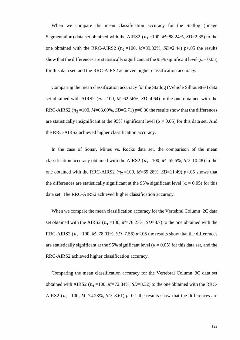
122
When we compare the mean classification accuracy for the Statlog (Image
Segmentation) data set obtained with the AIRS2 (𝑛1 =100, M=88.24%, SD=2.35) to the
one obtained with the RRC-AIRS2 (𝑛2 =100, M=89.32%, SD=2.44) p<.05 the results
show that the differences are statistically significant at the 95% significant level (α = 0.05)
for this data set, and the RRC-AIRS2 achieved higher classification accuracy.
Comparing the mean classification accuracy for the Statlog (Vehicle Silhouettes) data
set obtained with AIRS2 (𝑛1 =100, M=62.56%, SD=4.64) to the one obtained with the
RRC-AIRS2 (𝑛2 =100, M=63.09%, SD=5.71) p=0.36 the results show that the differences
are statistically insignificant at the 95% significant level (α = 0.05) for this data set. And
the RRC-AIRS2 achieved higher classification accuracy.
In the case of Sonar, Mines vs. Rocks data set, the comparison of the mean
classification accuracy obtained with the AIRS2 (𝑛1 =100, M=65.6%, SD=10.48) to the
one obtained with the RRC-AIRS2 (𝑛2 =100, M=69.28%, SD=11.49) p<.05 shows that
the differences are statistically significant at the 95% significant level (α = 0.05) for this
data set. The RRC-AIRS2 achieved higher classification accuracy.
When we compare the mean classification accuracy for the Vertebral Column_2C data
set obtained with the AIRS2 (𝑛1 =100, M=76.23%, SD=8.7) to the one obtained with the
RRC-AIRS2 (𝑛2 =100, M=78.01%, SD=7.56) p<.05 the results show that the differences
are statistically significant at the 95% significant level (α = 0.05) for this data set, and the
RRC-AIRS2 achieved higher classification accuracy.
Comparing the mean classification accuracy for the Vertebral Column_3C data set
obtained with AIRS2 (𝑛1 =100, M=72.84%, SD=8.32) to the one obtained with the RRC-
AIRS2 (𝑛2 =100, M=74.23%, SD=8.61) p=0.1 the results show that the differences are

123
statistically insignificant at the 95% significant level (α = 0.05) for this data set. However
the RRC-AIRS2 achieved higher classification accuracy.
In the case of Wisconsin Breast Cancer Data Set (WBCD) (Original) data set, the
comparison of the mean classification accuracy obtained with the AIRS2 (𝑛1 =100,
M=96.58%, SD=2.19) to the one obtained with the RRC-AIRS2 (𝑛2 =100, M=96.56%,
SD=2.24) p=0.93 shows that the differences are statistically significant at the 95%
significant level (α = 0.05) for this data set. The AIRS2 achieved higher classification
accuracy.
Figure 4.14 illustrates a graphical comparison of classification accuracy on benchmark
data sets obtained with AIRS2 and RRC-AIRS2 algorithms. As it can be seen, RRC-
AIRS2 has increased the classification accuracy on 12 out of 15 benchmark data sets.
124
Figure 4.14: Comparison of Classification Accuracy AIRS2 versus RRC-AIRS2 on
benchmark data sets
In general we can conclude that RRC-AIRS2 has achieved higher classification
accuracy than the AIRS2 on almost all (12 out of 15) benchmark data sets. Only in four
cases the differences are statistically significant in favour of RRC-AIRS2, while in other
cases the differences are statistically insignificant.
0.00
10.00
20.00
30.00
40.00
50.00
60.00
70.00
80.00
90.00
100.00
Balan
ce Scale
Breast C
ancer W
iscon
sin (D
iagno
stic)
Co
ntact Le
nse
s
Ion
osp
here
Iris
Liver Diso
rders
Lun
g Can
cer
Pim
a Ind
ians
Statlog (H
eart)
Statlog (Im
age Se
gmen
tation
)
Statlog (V
ehicle Silh
ou
ettes)
Son
ar, Min
es vs. Ro
cks
Verte
bral C
olu
mn
_2C
Verte
bral C
olu
mn
_3C
Wisco
nsin
Breast C
ancer D
ata Set (W
BC
D) (O
riginal)
Acc
ura
cy
Data sets
AIRS2 RRC-AIRS2
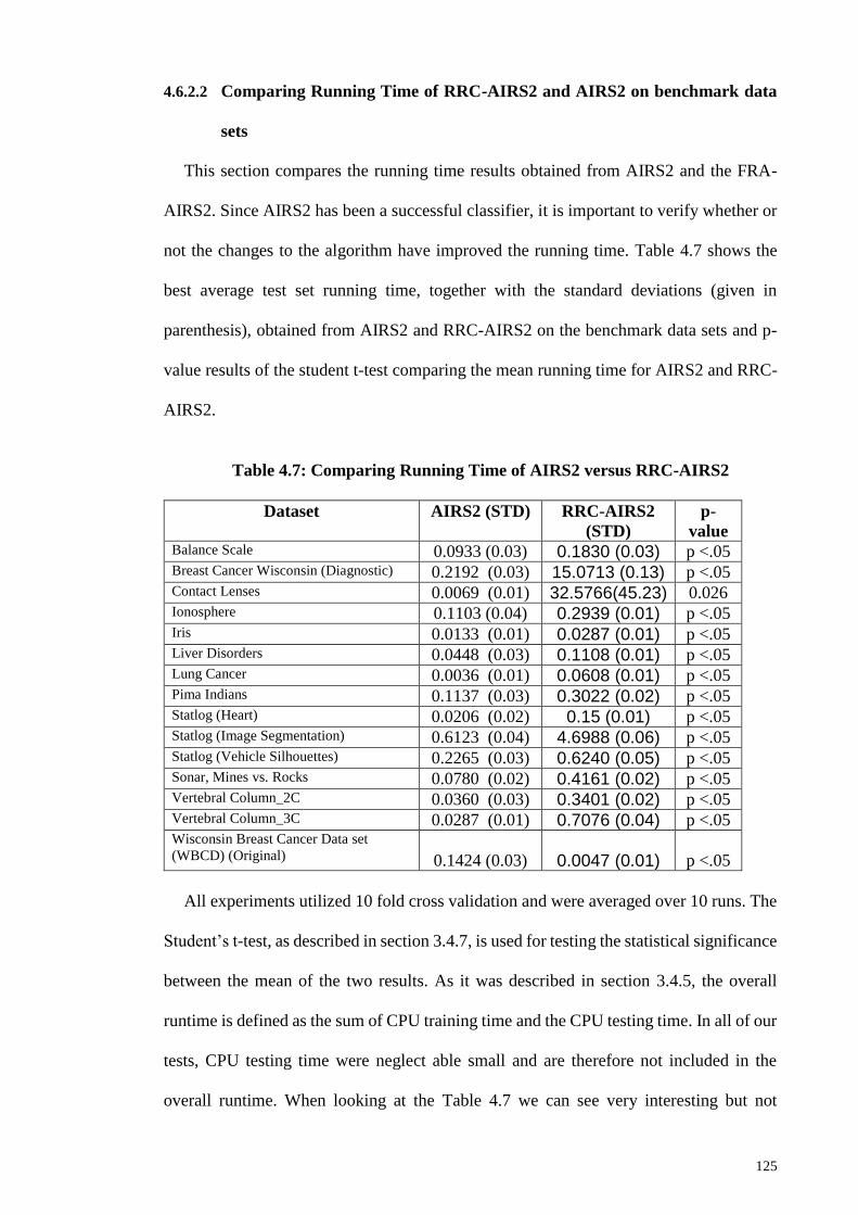
125
4.6.2.2 Comparing Running Time of RRC-AIRS2 and AIRS2 on benchmark data
sets
This section compares the running time results obtained from AIRS2 and the FRA-
AIRS2. Since AIRS2 has been a successful classifier, it is important to verify whether or
not the changes to the algorithm have improved the running time. Table 4.7 shows the
best average test set running time, together with the standard deviations (given in
parenthesis), obtained from AIRS2 and RRC-AIRS2 on the benchmark data sets and p-
value results of the student t-test comparing the mean running time for AIRS2 and RRC-
AIRS2.
Table 4.7: Comparing Running Time of AIRS2 versus RRC-AIRS2
Dataset AIRS2 (STD) RRC-AIRS2
(STD)
p-
value Balance Scale 0.0933 (0.03) 0.1830 (0.03) p <.05 Breast Cancer Wisconsin (Diagnostic) 0.2192 (0.03) 15.0713 (0.13) p <.05 Contact Lenses 0.0069 (0.01) 32.5766(45.23) 0.026 Ionosphere 0.1103 (0.04) 0.2939 (0.01) p <.05 Iris 0.0133 (0.01) 0.0287 (0.01) p <.05 Liver Disorders 0.0448 (0.03) 0.1108 (0.01) p <.05 Lung Cancer 0.0036 (0.01) 0.0608 (0.01) p <.05 Pima Indians 0.1137 (0.03) 0.3022 (0.02) p <.05 Statlog (Heart) 0.0206 (0.02) 0.15 (0.01) p <.05 Statlog (Image Segmentation) 0.6123 (0.04) 4.6988 (0.06) p <.05 Statlog (Vehicle Silhouettes) 0.2265 (0.03) 0.6240 (0.05) p <.05 Sonar, Mines vs. Rocks 0.0780 (0.02) 0.4161 (0.02) p <.05 Vertebral Column_2C 0.0360 (0.03) 0.3401 (0.02) p <.05 Vertebral Column_3C 0.0287 (0.01) 0.7076 (0.04) p <.05 Wisconsin Breast Cancer Data set
(WBCD) (Original) 0.1424 (0.03) 0.0047 (0.01)
p <.05
All experiments utilized 10 fold cross validation and were averaged over 10 runs. The
Student’s t-test, as described in section 3.4.7, is used for testing the statistical significance
between the mean of the two results. As it was described in section 3.4.5, the overall
runtime is defined as the sum of CPU training time and the CPU testing time. In all of our
tests, CPU testing time were neglect able small and are therefore not included in the
overall runtime. When looking at the Table 4.7 we can see very interesting but not

126
surprising results; while only in case of (Wisconsin Breast Cancer Data set (WBCD)
(Original)) RRC-AIRS2 required lower running time for the classification, it required
higher running time in all other 14 out of 15 cases.
The results are not surprising, because when we look at Table 4.6 in section 4.6.2.1,
we can see that RRC-AIRS2 was able to achieve higher classification accuracy than
AIRS2 in 13 out of 15 cases, whereby the results were statistically significant only in 5
cases. It is well known that the price for higher classification is usually higher running
time.
4.6.3 Evaluation of FSR-AIRS2
This section compares the results obtained from AIRS (AIRS2) and the FSR-AIRS2.
Since AIRS2 has been a successful classifier, it is important to verify whether or not the
changes to the algorithm have improved the classification accuracy.
4.6.3.1 Classification Accuracy of FSR-AIRS2 versus AIRS2
Table 4.8 shows the best average test set accuracies, together with the standard
deviations (given in parenthesis), obtained from AIRS2 and FSR-AIRS2 on the
benchmark data sets and p-value results of the student t-test comparing the mean
accuracies for AIRS2 and FSR-AIRS2.
All experiments utilized 10 fold cross validation and were averaged over 10 runs. The
Student’s t-test, as described in section 3.4.7, is used for testing the statistical significance
between the mean of the two results.
Table 4.8 shows that the changes made to the AIRS2 algorithm have improved the
classification accuracy. Results show that the differences in accuracy for almost all
benchmark are significant at the 95% significant level (α = 0.05) based on a two-tailed
student’s t-test as described in section 3.4.7.

127
Table 4.8: Comparative Average Accuracies
Training Set AIRS2 (STD) FSR-AIRS2
(STD)
p-value
Balance Scale 86.83% (3.14) 94.25% (3.30) p < 0.05
Breast Cancer Wisconsin
(Diagnostic)
96.17% (2.32) 100% (0.00) p < 0.05
Contact Lenses 82.83% (22.53) 83.17% (22.79) 0.92
Ionosphere 86.04% (4.84) 100% (0.00) p < 0.05
Iris 94.67% (5.36) 98.00% (6.03) p < 0.05
Liver Disorders 59.80% (8.18) 79.17% (9.49) p < 0.05
Lung Cancer 41.83% (26.64) 96.00% (12.34) p < 0.05
Pima Indians 74.41% (5.11) 99.54% (1.64) p < 0.05
Statlog (Heart) 77.48% (8.42) 84.44% (9.71) p < 0.05
Statlog (Image Segmentation) 88.24% (2.35) 91.05% (9.40) p < 0.05
Statlog (Vehicle Silhouettes) 62.56% (4.64) 79.79% (9.21) p < 0.05
Sonar, Mines vs. Rocks 65.60% (10.48) 98.08% (4.55) p < 0.05
Vertebral Column_2C 76.23% (8.70) 89.36% (6.06) p < 0.05
Vertebral Column_3C 72.84% (8.32) 87.19% (8.08) p < 0.05
Wisconsin Breast Cancer Data
Set (WBCD) (Original)
96.58% (2.19) 100% (0.00) p < 0.05
When we compare the mean classification accuracy for the Balance Scale data set
obtained with the AIRS2 (𝑛1 =100, M=86.83%, SD=3.14) to the one obtained with FSR-
AIRS2 (𝑛2 =100, M=94.5%, SD=3.3) p<.05 the results show that the differences are
statistically significant at the 95% significant level (α = 0.05) for this data set. The FSR-
AIRS2 achieved significantly higher classification accuracy.
Comparing the mean classification accuracy for the Breast Cancer Wisconsin
(Diagnostic) data set obtained with AIRS2 (𝑛1 =100, M=96.17%, SD=2.32) to the one
obtained with the FSR-AIRS2 (𝑛2 =100, M=100%, SD=0.0) p<.05 the results show that
the differences are statistically significant at the 95% significant level (α = 0.05) for this
data set and the FSR-AIRS2 achieved significantly higher classification accuracy.
In the case of Contact Lenses data set, the comparison of the mean classification
accuracy obtained with the AIRS2 (𝑛1 =100, M=82.83%, SD=22.53) to the one obtained
with the FSR-AIRS2 (𝑛2 =100, M=83.17%, SD=22.79) p=.92 shows that the differences

128
are statistically insignificant at the 95% significant level (α = 0.05) for this data set.
However, the FSR-AIRS2 achieved slightly higher classification accuracy.
When we compare the mean classification accuracy for the Ionosphere data set
obtained with the AIRS2 (𝑛1 =100, M=86.04%, SD=4.84) to the one obtained with the
FSR-AIRS2 (𝑛2 =100, M=100%, SD=0.0) p<.05 the results show that the differences are
statistically significant at the 95% significant level (α = 0.05) for this data set and the
FSR-AIRS2 achieved significantly higher classification accuracy.
Comparing the mean classification accuracy for the Iris data set obtained with the
AIRS2 (𝑛1 =100, M=94.67%, SD=5.36) to the one obtained with the FSR-AIRS2
(𝑛2 =100, M=98.00%, SD=6.03) p<.05 the results show that the differences are
statistically significant at the 95% significant level (α = 0.05) for this data set and the
FSR-AIRS2 achieved significantly higher classification accuracy.
In the case of Liver Disorders data set, the comparison of the mean classification
accuracy obtained with the AIRS2 (𝑛1 =100, M=59.8%, SD=8.18) to the one obtained
with the FSR-AIRS2 (𝑛2 =100, M=79.17%, SD=9.49) p<.05 the results show that the
differences are statistically significant at the 95% significant level (α = 0.05) for this data
set and the FSR-AIRS2 achieved significantly higher classification accuracy.
When we compare the mean classification accuracy for the Lung Cancer data set
obtained with the AIRS2 (𝑛1 =100, M=41.83%, SD=26.64) to the one obtained with FSR-
AIRS2 (𝑛2 =100, M=96.00%, SD=12.34) p<.05 the results show that the differences are
statistically significant at the 95% significant level (α = 0.05) for this data set and the
FSR-AIRS2 achieved significantly higher classification accuracy.
Comparing the mean classification accuracy for the Pima Indians data set obtained
with AIRS2 (𝑛1 =100, M=74.41%, SD=5.11) to the one obtained with FSR-AIRS2

129
(𝑛2 =100, M=99.54%, SD=1.64) p<.05 the results show that the differences are
statistically significant at the 95% significant level (α = 0.05) for this data set and the
FSR-AIRS2 achieved significantly higher classification accuracy.
In the case of Statlog (Heart) data set, the comparison of the mean classification
accuracy obtained with the AIRS2 (𝑛1 =100, M=77.48%, SD=8.42) to the one obtained
with the FSR-AIRS2 (𝑛2 =100, M=84.44%, SD=9.71) p<.05 the results show that the
differences are statistically significant at the 95% significant level (α = 0.05) for this data
set and the FSR-AIRS2 achieved significantly higher classification accuracy.
When we compare the mean classification accuracy for the Statlog (Image
Segmentation) data set obtained with the AIRS2 (𝑛1 =100, M=88.24%, SD=2.35) to the
one obtained with the FSR-AIRS2 (𝑛2 =100, M=91.05%, SD=9.40) p<.05 the results
show that the differences are statistically significant at the 95% significant level (α = 0.05)
for this data set and the FSR-AIRS2 achieved significantly higher classification accuracy.
Comparing the mean classification accuracy for the Statlog (Vehicle Silhouettes) data
set obtained with AIRS2 (𝑛1 =100, M=62.56%, SD=4.64) to the one obtained with the
FSR-AIRS2 (𝑛2 =100, M=79.79%, SD=9.21) p<.05 the results show that the differences
are statistically significant at the 95% significant level (α = 0.05) for this data set and the
FSR-AIRS2 achieved significantly higher classification accuracy.
In the case of Sonar, Mines vs. Rocks data set, the comparison of the mean
classification accuracy obtained with the AIRS2 (𝑛1 =100, M=65.6%, SD=10.48) to the
one obtained with the FSR-AIRS2 (𝑛2 =100, M=98.08%, SD=4.55) p<.05 the results
show that the differences are statistically significant at the 95% significant level (α = 0.05)
for this data set and the FSR-AIRS2 achieved significantly higher classification accuracy.

130
When we compare the mean classification accuracy for the Vertebral Column_2C data
set obtained with the AIRS2 (𝑛1 =100, M=76.23%, SD=8.7) to the one obtained with the
FSR-AIRS2 (𝑛2 =100, M=89.36%, SD=6.06) p<.05 the results show that the differences
are statistically significant at the 95% significant level (α = 0.05) for this data set and the
FSR-AIRS2 achieved significantly higher classification accuracy.
Comparing the mean classification accuracy for the Vertebral Column_3C data set
obtained with AIRS2 (𝑛1 =100, M=72.84%, SD=8.32) to the one obtained with the FSR-
AIRS2 (𝑛2 =100, M=87.19%, SD=8.08) p<.05 the results show that the differences are
statistically significant at the 95% significant level (α = 0.05) for this data set and the
FSR-AIRS2 achieved significantly higher classification accuracy.
In the case of Wisconsin Breast Cancer Data Set (WBCD) (Original) data set, the
comparison of the mean classification accuracy obtained with the AIRS2 (𝑛1 =100,
M=96.58%, SD=2.19) to the one obtained with the FSR-AIRS2 (𝑛2 =100, M=100%,
SD=0.0) p<.05 the results show that the differences are statistically significant at the 95%
significant level (α = 0.05) for this data set and the FSR-AIRS2 achieved significantly
higher classification accuracy.
In general, since α ≥ p on all bench mark data sets, it can be concluded that
modifications introduced in FSR-AIRS2 appear to have positive effect on the
classification accuracy of the classifier. The comparison with AIRS2 shows that FSR-
AIRS2 has statistically significantly increased the classification accuracy on almost all
(14 out of 15) benchmark data sets.
Figure 4.15 illustrates a graphical comparison of classification accuracy on benchmark
data sets obtained with AIRS2 and FSR-AIRS2 algorithms. Figure 4.15 shows the
superiority of FSR-AIRS2 over AIRS2.

131
Figure 4.15: Comparison of Classification Accuracy AIRS2 versus FSR-AIRS2 on
benchmark data sets.
4.6.3.2 Classification Accuracy of FSR-AIRS2 versus Other Well-known Classifiers
Table 4.9 shows the best average test set accuracies, together with the standard
deviations (given in parenthesis) obtained from FSR-AIRS2 and other well-known
classifiers: 1-KNN, 7-KNN, C4.5/J48, CLONALG, Immunos99, LibSVM, Logistic,
MLP, Naïve Bayes, RBF Network, SMO, and SMO2 on the Balance Scale data set.
0
10
20
30
40
50
60
70
80
90
100
Balan
ce Scale
Bre
ast Can
cer W
iscon
sin (D
iagno
stic)
Co
ntact Le
nses
Ion
osp
here
Iris
Liver Diso
rders
Lun
g Can
cer
Pim
a Ind
ians
Statlog (H
eart)
Statlog (Im
age Segm
entatio
n)
Statlog (V
ehicle
Silho
uette
s)
Son
ar, Min
es vs. Ro
cks
Ve
rtebral C
olu
mn
_2C
Ve
rtebral C
olu
mn
_3C
Wisco
nsin
Breast C
ancer D
ata Set (W
BC
D) (O
riginal)
Acc
ura
cy
Data Sets
AIRS2
FSR-AIRS2

132
All experiments utilized 10 fold cross validation and were averaged over 10 runs. The
top three classifiers for the data set are presented next.
Table 4.9: Comparison of Classification Results of FSR-AIRS2 and Benchmark
Classifiers on Balance Scale Data Set
FSR-
AIRS2
1KNN 7KNN C4.5/J48 CLONALG Immunos99
94.25
(3.30)
86.72
(2.71)
89.71
(2.33)
77.82
(3.42)
77.46
(5.68)
67.12
(9.59)
LibSVM Logistic MLP NBayes RBF Netw. SMO
89.87
(1.67)
89.44 (3.29)
90.69
(3.04)
90.53
(1.67)
86.18
(3.76)
87.57
(2.49)
SMO2
91.38
(1.93)
Figure 4.16 illustrates a comparative graph of various classifiers on the Balance Scale
data set. Results show that for this data set FSR-AIRS2 achieved the highest classification
accuracy of 94.25% followed by SMO2 and MLP with 91.38% and 90.69% respectively.
These results show that the proposed model compares well with other well-known
classifiers on this data set.
Figure 4.16: Comparison of Balance Scale Accuracy Results
Table 4.10 shows the best average test set accuracies, together with the standard
deviations (given in parenthesis) obtained from FSR-AIRS2 and other well-known
0.0010.0020.0030.0040.0050.0060.0070.0080.0090.00
100.00
Acc
ura
cy
Classifiers

133
classifiers: 1-KNN, 7-KNN, C4.5/J48, CLONALG, Immunos99, LibSVM, Logistic,
MLP, Naïve Bayes, RBF Network, SMO, and SMO2 on the Breast Cancer Wisconsin
(Diagnostic) data sets.
All experiments utilized 10 fold cross validation and were averaged over 10 runs. The
top three classifiers for the data set are presented next.
Table 4.10: Comparison of Classification Results of FSR-AIRS2 and
Benchmark Classifiers on Breast Cancer Wisconsin (Diagnostic) Data Set
FSR-
AIRS2
1KNN 7KNN C4.5/J48 CLONALG Immunos99
100.00
(0.00)
95.64
(2.32)
97.19
(2.10)
93.27
(3.55)
88.82
(4.94)
87.77
(4.10)
LibSVM Logistic MLP NBayes RBF Netw. SMO
62.74
(0.70)
94.46
(3.53)
96.61
(2.45)
93.31
(3.30)
94.22
(3.15)
97.54
(1.85)
SMO2
98.00
(1.82)
Figure 4.17 illustrates a comparative graph of various classifiers on the Breast Cancer
Wisconsin (Diagnostic) data set. Here, the highest accuracy was obtained by FSR-AIRS2
with 100% followed by SMO2 and SMO with 98% and 97.54% respectively.
These results show that the proposed model compares well with other well-known
classifiers. These results show that the proposed model performs better or compares well
with other well-known classifiers on this data set.

134
Figure 4.17: Comparison of Breast Cancer Wisconsin (Diagnostic) Accuracy
Results
Table 4.11 shows the best average test set accuracies, together with the standard
deviations (given in parenthesis) obtained from FSR-AIRS2 and other well-known
classifiers: 1-KNN, 7-KNN, C4.5/J48, CLONALG, Immunos99, LibSVM, Logistic,
MLP, Naïve Bayes, RBF Network, SMO, and SMO2 on the Contact Lenses data sets. All
experiments utilized 10 fold cross validation and were averaged over 10 runs. The top
three classifiers for the data set are presented next.
Table 4.11: Comparison of Classification Results of FSR-AIRS2 and
Benchmark Classifiers on Contact Lenses Data Set
FSR-
AIRS2
1KNN 7KNN C4.5/J48 CLONALG Immunos99
83.17
(22.79)
80.50
(25.19)
63.33
(23.21)
83.50
(22.42)
65.67
(30.87)
58.67
(31.74)
LibSVM Logistic MLP NBayes RBF Netw. SMO
63.83
(23.46)
67.33
(30.05)
74.50
(27.73)
76.17
(25.54)
76.67
(27.22)
72.50
(26.42)
SMO2
76.50
(27.74)
Figure 4.18 illustrates a comparative graph of various classifiers on the Contact Lenses
data set. C4.5/J48 achieved the highest classification accuracy of 83.50% for this data
set, followed by FSR-AIRS2 and 1KNN with 83.17% and 80.5% respectively on the same
0.0020.0040.0060.0080.00
100.00
Acc
ura
cyClassifiers

135
data set. The FSR-AIRS2 algorithm performs only slightly worse than the C4.5/J48.
These results show that the proposed model compares well with other well-known
classifiers.
Figure 4.18: Comparison of Contact Lenses Accuracy Results
Table 4.12 shows the best average test set accuracies, together with the standard
deviations (given in parenthesis) obtained from FSR-AIRS2 and other well-known
classifiers: 1-KNN, 7-KNN, C4.5/J48, CLONALG, Immunos99, LibSVM, Logistic,
MLP, Naïve Bayes, RBF Network, SMO, and SMO2 on the Ionosphere data set. All
experiments utilized 10 fold cross validation and were averaged over 10 runs. The top
three classifiers for the data set are presented next.
Table 4.12: Comparison of Classification Results of FSR-AIRS2 and
Benchmark Classifiers on Ionosphere Data Set
FSR-
AIRS2
1KNN 7KNN C4.5/J48 CLONALG Immunos99
100.00
(0.00)
87.10
(5.12)
84.30
(4.86)
89.74
(4.38)
77.22
(10.65)
71.17
(4.16)
LibSVM Logistic MLP NBayes RBF Netw. SMO
93.05
(3.95)
87.72
(5.57)
91.06
(4.86)
82.17
(6.14)
91.74
(4.62)
88.07
(5.32)
SMO2
90.69
(4.68)
0.00
20.00
40.00
60.00
80.00
100.00A
ccu
racy
Classifiers

136
Figure 4.19 illustrates a comparative graph of various classifiers on the Ionosphere
data set. For this data set, the FSR-AIRS2 algorithm achieved the highest classification
accuracy of 100% followed by LibSVM and RBF with 93.05% and 91.74% respectively.
These results show that the proposed model performs better or compares well with other
well-known classifiers on this data set.
Figure 4.19: Comparison of Ionosphere Accuracy Results
Table 4.13 shows the best average test set accuracies, together with the standard
deviations (given in parenthesis) obtained from FSR-AIRS2 and other well-known
classifiers: 1-KNN, 7-KNN, C4.5/J48, CLONALG, Immunos99, LibSVM, Logistic,
MLP, Naïve Bayes, RBF Network, SMO, and SMO2 on the Iris data set. All experiments
utilized 10 fold cross validation and were averaged over 10 runs. The top three classifiers
for the data set are presented next.
0.00
10.00
20.00
30.00
40.00
50.00
60.00
70.00
80.00
90.00
100.00
Acc
ura
cy
Classifiers
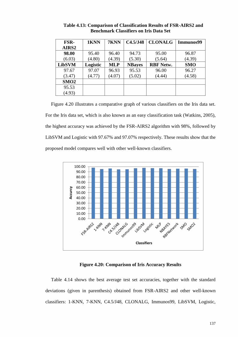
137
Table 4.13: Comparison of Classification Results of FSR-AIRS2 and
Benchmark Classifiers on Iris Data Set
FSR-
AIRS2
1KNN 7KNN C4.5/J48 CLONALG Immunos99
98.00
(6.03)
95.40
(4.80)
96.40
(4.39)
94.73
(5.30)
95.00
(5.64)
96.87
(4.39)
LibSVM Logistic MLP NBayes RBF Netw. SMO
97.67
(3.47)
97.07
(4.77)
96.93
(4.07)
95.53
(5.02)
96.00
(4.44)
96.27
(4.58)
SMO2
95.53
(4.93)
Figure 4.20 illustrates a comparative graph of various classifiers on the Iris data set.
For the Iris data set, which is also known as an easy classification task (Watkins, 2005),
the highest accuracy was achieved by the FSR-AIRS2 algorithm with 98%, followed by
LibSVM and Logistic with 97.67% and 97.07% respectively. These results show that the
proposed model compares well with other well-known classifiers.
Figure 4.20: Comparison of Iris Accuracy Results
Table 4.14 shows the best average test set accuracies, together with the standard
deviations (given in parenthesis) obtained from FSR-AIRS2 and other well-known
classifiers: 1-KNN, 7-KNN, C4.5/J48, CLONALG, Immunos99, LibSVM, Logistic,
0.00
10.00
20.00
30.00
40.00
50.00
60.00
70.00
80.00
90.00
100.00
Acc
urc
y
Classifiers

138
MLP, Naïve Bayes, RBF Network, SMO, and SMO2 on the Liver Disorders data set. All
experiments utilized 10 fold cross validation and were averaged over 10 runs. The top
three classifiers for the data set are presented next.
Table 4.14: Comparison of Classification Results of FSR-AIRS2 and
Benchmark Classifiers on Liver Disorders Data Set
FSR-
AIRS2
1KNN 7KNN C4.5/J48 CLONALG Immunos99
79.17
(9.49)
62.22
(8.18)
62.63
(7.92)
65.84
(7.40)
56.55
(8.19)
51.34
(6.69)
LibSVM Logistic MLP NBayes RBF Netw. SMO
59.37
(2.28)
68.72
(7.98)
57.98
(0.84)
54.89
(8.83)
65.09
(8.88)
57.98
(1.26)
SMO2
58.82
(3.11)
Figure 4.21 illustrates a comparative graph of various classifiers on the Liver Disorders
data set. In case of Liver Disorders, the highest accuracy of 79.17% was obtained with
FSR-AIRS2 followed by Logistic and C4.5/J48 with 68.72% and 65.84% respectively.
These results show that the proposed model performed better other well-known classifiers
on this data set.
Figure 4.21: Comparison of Liver Disorders Accuracy Results
0.0010.0020.0030.0040.0050.0060.0070.0080.0090.00
100.00
Acc
ura
cy
Classifiers
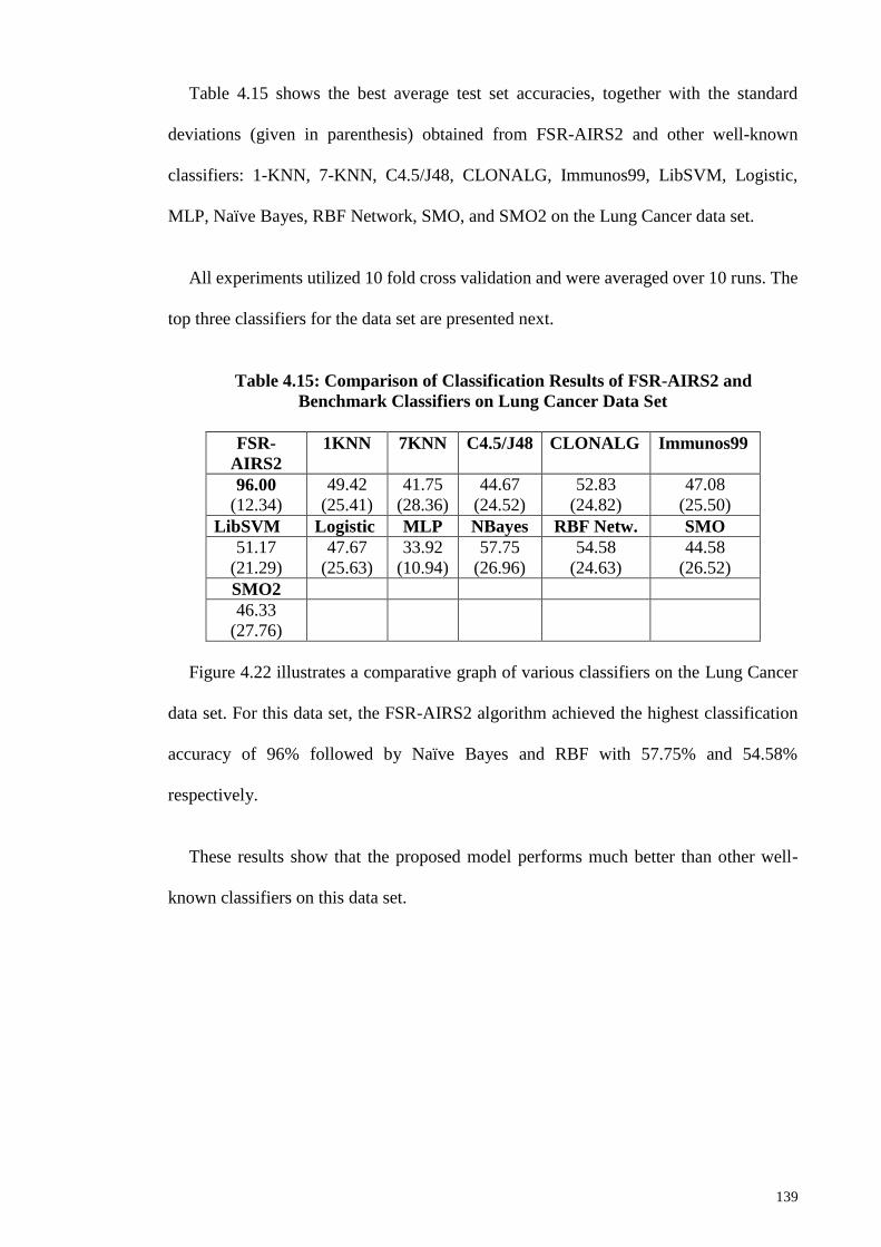
139
Table 4.15 shows the best average test set accuracies, together with the standard
deviations (given in parenthesis) obtained from FSR-AIRS2 and other well-known
classifiers: 1-KNN, 7-KNN, C4.5/J48, CLONALG, Immunos99, LibSVM, Logistic,
MLP, Naïve Bayes, RBF Network, SMO, and SMO2 on the Lung Cancer data set.
All experiments utilized 10 fold cross validation and were averaged over 10 runs. The
top three classifiers for the data set are presented next.
Table 4.15: Comparison of Classification Results of FSR-AIRS2 and
Benchmark Classifiers on Lung Cancer Data Set
FSR-
AIRS2
1KNN 7KNN C4.5/J48 CLONALG Immunos99
96.00
(12.34)
49.42
(25.41)
41.75
(28.36)
44.67
(24.52)
52.83
(24.82)
47.08
(25.50)
LibSVM Logistic MLP NBayes RBF Netw. SMO
51.17
(21.29)
47.67
(25.63)
33.92
(10.94)
57.75
(26.96)
54.58
(24.63)
44.58
(26.52)
SMO2
46.33
(27.76)
Figure 4.22 illustrates a comparative graph of various classifiers on the Lung Cancer
data set. For this data set, the FSR-AIRS2 algorithm achieved the highest classification
accuracy of 96% followed by Naïve Bayes and RBF with 57.75% and 54.58%
respectively.
These results show that the proposed model performs much better than other well-
known classifiers on this data set.
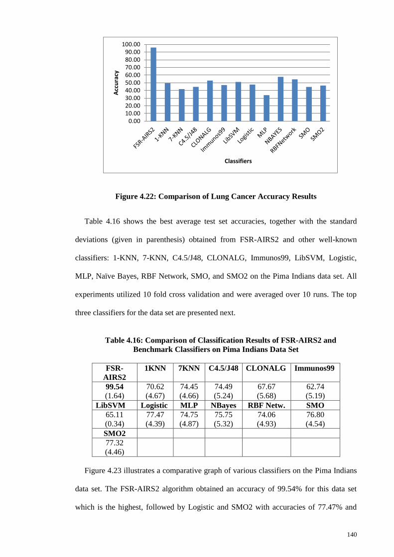
140
Figure 4.22: Comparison of Lung Cancer Accuracy Results
Table 4.16 shows the best average test set accuracies, together with the standard
deviations (given in parenthesis) obtained from FSR-AIRS2 and other well-known
classifiers: 1-KNN, 7-KNN, C4.5/J48, CLONALG, Immunos99, LibSVM, Logistic,
MLP, Naïve Bayes, RBF Network, SMO, and SMO2 on the Pima Indians data set. All
experiments utilized 10 fold cross validation and were averaged over 10 runs. The top
three classifiers for the data set are presented next.
Table 4.16: Comparison of Classification Results of FSR-AIRS2 and
Benchmark Classifiers on Pima Indians Data Set
FSR-
AIRS2
1KNN 7KNN C4.5/J48 CLONALG Immunos99
99.54
(1.64)
70.62
(4.67)
74.45
(4.66)
74.49
(5.24)
67.67
(5.68)
62.74
(5.19)
LibSVM Logistic MLP NBayes RBF Netw. SMO
65.11
(0.34)
77.47
(4.39)
74.75
(4.87)
75.75
(5.32)
74.06
(4.93)
76.80
(4.54)
SMO2
77.32
(4.46)
Figure 4.23 illustrates a comparative graph of various classifiers on the Pima Indians
data set. The FSR-AIRS2 algorithm obtained an accuracy of 99.54% for this data set
which is the highest, followed by Logistic and SMO2 with accuracies of 77.47% and
0.0010.0020.0030.0040.0050.0060.0070.0080.0090.00
100.00
Acc
ura
cy
Classifiers

141
77.32% respectively. These results show that the proposed model performs much better
than other well-known classifiers on this data set.
Figure 4.23: Comparison of Pima Indians Accuracy Results
Table 4.17 shows the best average test set accuracies, together with the standard
deviations (given in parenthesis) obtained from FSR-AIRS2 and other well-known
classifiers: 1-KNN, 7-KNN, C4.5/J48, CLONALG, Immunos99, LibSVM, Logistic,
MLP, Naïve Bayes, RBF Network, SMO, and SMO2 on the Statlog (Heart) data set. All
experiments utilized 10 fold cross validation and were averaged over 10 runs. The top
three classifiers for the data set are presented next.
Table 4.17: Comparison of Classification Results of FSR-AIRS2 and
Benchmark Classifiers on Statlog (Heart) Data Set
FSR-
AIRS2
1KNN 7KNN C4.5/J48 CLONALG Immunos99
84.44
(9.71)
76.15
(8.46)
80.81
(6.73)
78.15
(7.42)
63.26
(7.66)
65.26
(8.61)
LibSVM Logistic MLP NBayes RBF Netw. SMO
55.93
(1.12)
83.67
(6.43)
55.56
(0.00)
83.59
(5.98)
83.11
(6.50)
83.89
(6.62)
SMO2
81.22
(6.62)
0.0010.0020.0030.0040.0050.0060.0070.0080.0090.00
100.00
Acc
ura
cy
Classifiers
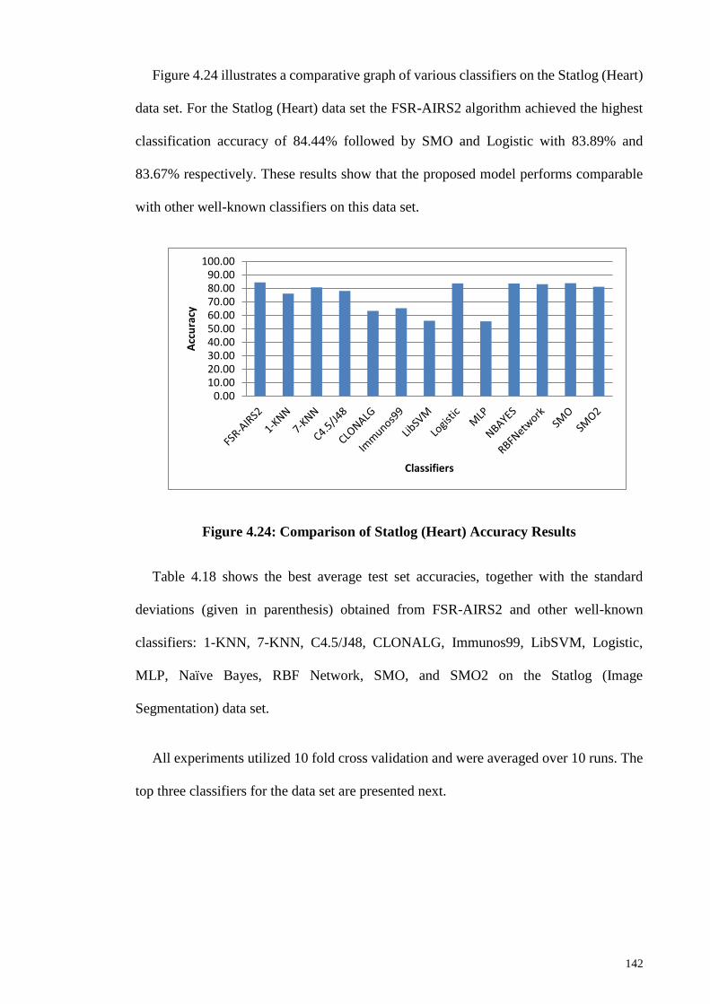
142
Figure 4.24 illustrates a comparative graph of various classifiers on the Statlog (Heart)
data set. For the Statlog (Heart) data set the FSR-AIRS2 algorithm achieved the highest
classification accuracy of 84.44% followed by SMO and Logistic with 83.89% and
83.67% respectively. These results show that the proposed model performs comparable
with other well-known classifiers on this data set.
Figure 4.24: Comparison of Statlog (Heart) Accuracy Results
Table 4.18 shows the best average test set accuracies, together with the standard
deviations (given in parenthesis) obtained from FSR-AIRS2 and other well-known
classifiers: 1-KNN, 7-KNN, C4.5/J48, CLONALG, Immunos99, LibSVM, Logistic,
MLP, Naïve Bayes, RBF Network, SMO, and SMO2 on the Statlog (Image
Segmentation) data set.
All experiments utilized 10 fold cross validation and were averaged over 10 runs. The
top three classifiers for the data set are presented next.
0.0010.0020.0030.0040.0050.0060.0070.0080.0090.00
100.00
Acc
ura
cy
Classifiers

143
Table 4.18: Comparison of Classification Results of FSR-AIRS2 and
Benchmark Classifiers on Statlog (Image Segmentation) Data Set
FSR-
AIRS2
1KNN 7KNN C4.5/J48 CLONALG Immunos99
91.05
(9.40) 97.15
(1.11)
94.89
(1.37)
96.79
(1.29)
57.46
(6.11)
54.17
(2.40)
LibSVM Logistic MLP NBayes RBF Netw. SMO
63.98
(3.47)
95.61
(1.50)
96.18
(1.17)
80.17
(2.12)
87.32
(2.15)
92.92
(1.52)
SMO2
94.68
(1.50)
Figure 4.25 illustrates a comparative graph of various classifiers on the Statlog (Image
Segmentation) data set. For this data set, the highest accuracy was obtained by 1KNN
with 97.15% followed by C4.5/J48 and MLP with 96.79% and 96.18% respectively.
These results show that the proposed model performs comparable with other well-known
classifiers on this data set.
Figure 4.25: Comparison of Statlog (Image Segmentation) Accuracy Results
Table 4.19 shows the best average test set accuracies, together with the standard
deviations (given in parenthesis) obtained from FSR-AIRS2 and other well-known
classifiers: 1-KNN, 7-KNN, C4.5/J48, CLONALG, Immunos99, LibSVM, Logistic,
MLP, Naïve Bayes, RBF Network, SMO, and SMO2 on the Statlog (Vehicle Silhouettes)
0.00
10.00
20.00
30.00
40.00
50.00
60.00
70.00
80.00
90.00
100.00
Acc
urc
y
Classifiers

144
data set. All experiments utilized 10 fold cross validation and were averaged over 10 runs.
The top three classifiers for the data set are presented next.
Table 4.19: Comparison of Classification Results of FSR-AIRS2 and
Benchmark Classifiers on Statlog (Vehicle Silhouettes) Data Set
FSR-
AIRS2
1KNN 7KNN C4.5/J4
8
CLONALG Immunos99
79.79
(9.21)
69.59
(3.77)
70.55
(4.01)
72.28
(4.32)
42.22
(6.55)
46.42
(4.98)
LibSVM Logistic MLP NBayes RBF Netw. SMO
30.06
(2.46)
79.80
(4.03) 81.11
(3.84)
44.68
(4.59)
65.34
(4.32)
74.08
(3.82)
SMO2
80.26
(3.69)
Figure 4.26 illustrates a comparative graph of various classifiers on the Statlog
(Vehicle Silhouettes) data set. The MLP obtained the highest accuracy of 81.11% for this
data set, followed by SMO2 and Logistic with accuracies of 80.26% and 79.8%
respectively. It should be noted that the MLP algorithm performs only slightly better than
the FSR-AIRS2 on this data set.
Figure 4.26: Comparison of Statlog (Vehicle Silhouettes) Accuracy Results
0.0010.0020.0030.0040.0050.0060.0070.0080.0090.00
100.00
Acc
ura
cy
Classifiers

145
Table 4.20 shows the best average test set accuracies, together with the standard
deviations (given in parenthesis) obtained from FSR-AIRS2 and other well-known
classifiers: 1-KNN, 7-KNN, C4.5/J48, CLONALG, Immunos99, LibSVM, Logistic,
MLP, Naïve Bayes, RBF Network, SMO, and SMO2 on the Sonar, Mines vs. Rocks data
set.
All experiments utilized 10 fold cross validation and were averaged over 10 runs. The
top three classifiers for the data set are presented next.
Table 4.20: Comparison of Classification Results of FSR-AIRS2 and
Benchmark Classifiers on Sonar, Mines vs. Rocks Data Set
FSR-
AIRS2
1KNN 7KNN C4.5/J4
8
CLONALG Immunos99
98.08
(4.55)
86.17
(8.45)
79.10
(8.98)
73.61
(9.34)
63.41
(9.95)
61.25
(9.60)
LibSVM Logistic MLP NBayes RBF Netw. SMO
64.99
(7.66)
72.47
(8.90)
81.61
(8.66)
67.71
(8.66)
72.62
(9.91)
76.60
(8.27)
SMO2
83.80
(7.84)
Figure 4.27 illustrates a comparative graph of various classifiers on the Sonar, Mines
vs. Rocks data set. For this data set, the FSR-AIRS2 algorithm achieved the highest
classification accuracy of 98.08% followed by 1KNN and SMO2 with 86.17% and 83.8%
respectively.
These results show that the proposed model performs much better than other well-
known classifiers on this data set.

146
Figure 4.27: Comparison of Sonar, Mines vs. Rocks Accuracy Results
Table 4.21 shows the best average test set accuracies, together with the standard
deviations (given in parenthesis) obtained from FSR-AIRS2 and other well-known
classifiers: 1-KNN, 7-KNN, C4.5/J48, CLONALG, Immunos99, LibSVM, Logistic,
MLP, Naïve Bayes, RBF Network, SMO, and SMO2 on the Vertebral Column_2C data
set. All experiments utilized 10 fold cross validation and were averaged over 10 runs. The
top three classifiers for the data set are presented next.
Table 4.21: Comparison of Classification Results of FSR-AIRS2 and
Benchmark Classifiers on Vertebral Column_2C Data Set
FSR-
AIRS2
1KNN 7KNN C4.5/J48 CLONALG Immunos99
89.36
(6.06)
81.06
(6.18)
78.19
(6.27)
81.39
(6.38)
75.19
(7.82)
72.97
(7.03)
LibSVM Logistic MLP NBayes RBF Netw. SMO
67.74
(0.00)
85.06
(5.85)
85.00
(6.24)
77.87
(6.82)
80.29
(6.72)
78.90
(6.06)
SMO2
79.39
(6.05)
Figure 4.28 illustrates a comparative graph of various classifiers on the Vertebral
Column_2C data set. The FSR-AIRS2 algorithm achieved the highest classification
accuracy of 89.36% followed by Logistic and MLP with 85.06% and 85% respectively.
0.0010.0020.0030.0040.0050.0060.0070.0080.0090.00
100.00
Acc
ura
cy
Classifiers
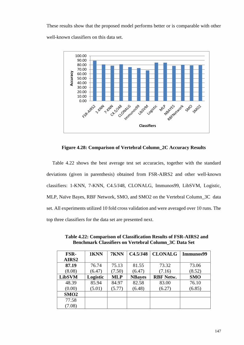
147
These results show that the proposed model performs better or is comparable with other
well-known classifiers on this data set.
Figure 4.28: Comparison of Vertebral Column_2C Accuracy Results
Table 4.22 shows the best average test set accuracies, together with the standard
deviations (given in parenthesis) obtained from FSR-AIRS2 and other well-known
classifiers: 1-KNN, 7-KNN, C4.5/J48, CLONALG, Immunos99, LibSVM, Logistic,
MLP, Naïve Bayes, RBF Network, SMO, and SMO2 on the Vertebral Column_3C data
set. All experiments utilized 10 fold cross validation and were averaged over 10 runs. The
top three classifiers for the data set are presented next.
Table 4.22: Comparison of Classification Results of FSR-AIRS2 and
Benchmark Classifiers on Vertebral Column_3C Data Set
FSR-
AIRS2
1KNN 7KNN C4.5/J48 CLONALG Immunos99
87.19
(8.08)
76.74
(6.47)
75.13
(7.50)
81.55
(6.47)
73.32
(7.16)
73.06
(8.52)
LibSVM Logistic MLP NBayes RBF Netw. SMO
48.39
(0.00)
85.94
(5.01)
84.97
(5.77)
82.58
(6.48)
83.00
(6.27)
76.10
(6.85)
SMO2
77.58
(7.08)
0.0010.0020.0030.0040.0050.0060.0070.0080.0090.00
100.00
Acc
ura
cy
Classifiers

148
Figure 4.29 illustrates a comparative graph of various classifiers on the Vertebral
Column_3C data set. For this data set the FSR-AIRS2 algorithm achieved the highest
classification accuracy of 87.19% followed by Logistic and MLP with 85.94% and
84.97% respectively.
These results show that the proposed model performs better or is comparable with
other well-known classifiers on this data set.
Figure 4.29: Comparison of Vertebral Column_3C Accuracy Results
Table 4.23 shows the best average test set accuracies, together with the standard
deviations (given in parenthesis) obtained from FSR-AIRS2 and other well-known
classifiers: 1-KNN, 7-KNN, C4.5/J48, CLONALG, Immunos99, LibSVM, Logistic,
MLP, Naïve Bayes, RBF Network, SMO, and SMO2 on the Wisconsin Breast Cancer
Data set (WBCD) (Original) data set.
All experiments utilized 10 fold cross validation and were averaged over 10 runs. The
top three classifiers for the data set are presented next.
0.00
10.00
20.00
30.00
40.00
50.00
60.00
70.00
80.00
90.00
100.00
Acc
ura
cy
Classifiers

149
Table 4.23: Comparison of Classification Results of FSR-AIRS2 and
Benchmark Classifiers on Wisconsin Breast Cancer Data set (WBCD) (Original)
Data Set
FSR-
AIRS2
1KNN 7KNN C4.5/J48 CLONALG Immunos99
100.00
(0.00)
95.18
(2.61)
96.80
(2.06)
94.58
(2.49)
61.51
(6.84)
67.90
(1.99)
LibSVM Logistic MLP NBayes RBF Netw. SMO
66.27
(0.98)
96.48
(2.17)
95.67
(2.21)
95.99
(2.25)
95.91
(2.48)
96.61
(2.02)
SMO2
96.47
(2.20)
Figure 4.30 illustrates a comparative graph of various classifiers on the Wisconsin
Breast Cancer Data Set (WBCD) (Original) data set. In case of this data set the highest
classification accuracy of 100% was obtained with the FSR-AIRS2 algorithm followed
by 7KNN and SMO with 96.8% and 96.61% respectively. These results show that the
proposed model performs better or is comparable with other well-known classifiers on
this data set.
Figure 4.30: Comparison of Wisconsin Breast Cancer Data Set (WBCD) (Original)
Accuracy Results
Results show that FSR-AIRS2 has achieved higher classification accuracy in 12 out of
15 cases and in one case it obtained the second highest accuracy on the benchmark data
0.00
10.00
20.00
30.00
40.00
50.00
60.00
70.00
80.00
90.00
100.00
Acc
ura
cy
Classifiers

150
sets. Results show that the FSR-AIRS2 algorithm performs comparatively well in relation
to other classifiers.
The results also suggest that the changes made in the proposed algorithm has
contributed toward the power of AIRS2, as Goodman et al. said major source of power
of the AIRS must lie in the way how it manages its memory cell population (Goodman et
al., 2003). Changes to resource allocation and resource competition mechanism on one
side and using a strong classifier such as SVM on the other hand have given the FSR-
AIRS2 this strength.
4.6.3.3 Data Reduction
One important feature of AIRS2 is its capability to perform the classification task with
the reduced number of data instances. Thus, it is essential to validate the performance of
the proposed algorithm.
Comparison of Evolved Memory Cells through AIRS2 and FRA-AIRS2
The goal of this section is to evaluate the application of the FRA method (introduced
in section 4.2) and verify whether or not this method improves the performance of the
AIRS2.
Table 4.24 presents the total number of instances, the best average test set evolved
memory cells, together with the standard deviations (given in parenthesis) and p-values
obtained from AIRS2 and FRA-AIRS2 on the benchmark data sets. All experiments
utilized 10 fold cross validation and were averaged over 10 runs. The two algorithms were
applied against fifteen data sets and the results are presented next. The results show the
number of memory cells (recognizer records) that were used for the classification. The
Goal of this evaluation is to verify which algorithm could do the classification task with

151
fewer numbers of memory cells (that is: number of records that are used for
classification).
Table 4.24: Comparison of Memory Cells Evolved with AIRS2 and FRA-AIRS2
Training Set Total
Instances
AIRS2
(STD)
FRA-AIRS2
(STD)
p-value
Balance Scale 625 248.68 (9.30) 285.23 (9.79) p < 0.05
Breast Cancer Wisconsin
(Diagnostic)
569 237.09 (10.47) 80.56 (5.60) p < 0.05
Contact Lenses 24 21.28 (0.75) 21.3 (0.75) 0.77
Ionosphere 351 140.78 (6.53) 55.75 (7.16) p < 0.05
Iris 150 47.11 (2.84) 42.36 (2.47) p < 0.05
Liver Disorders 345 196.7 (5.84) 102.95 (6.74) p < 0.05
Lung Cancer 32 15.66 (2.09) 20.51 (2.09) p < 0.05
Pima Indians 768 378.04 (11.24) 183.67 (11.17) p < 0.05
Statlog (Heart) 270 50.37 (6.21) 51.96 (6.02) p < 0.05
Statlog (Image
Segmentation)
2310 219.79 (11.71) 107.77 (7.81) p < 0.05
Statlog (Vehicle
Silhouettes)
846 354.88 (12.30) 132.94 (7.89) p < 0.05
Sonar, Mines vs. Rocks 208 143.33 (8.76) 61.69 (5.83) p < 0.05
Vertebral Column_2C 310 151.75 (6.28) 102.32 (9.26) p < 0.05
Vertebral Column_3C 310 153.52 (6.43) 104.51 (8.34) p < 0.05
Wisconsin Breast Cancer
Data Set (WBCD)
(Original)
699 227.82 (6.60) 214.74 (6.67) p < 0.05
When we compare the mean evolved memory cells for the Balance Scale data set
obtained from the AIRS2 (𝑛1 =100, M=248.68, SD=9.30) to the one obtained with the
FRA-AIRS2 (𝑛2 =100, M=258.23, SD=9.79) the results show that the differences in
average evolved memory cells are significant at the 95% significant level (α = 0.05) for
this data set using student’s t-test as described in section 3.4.7 The results suggest that
applying the FRA method could reduce the size of data set that is needed for classification
for this data set, however the AIRS2 performed slightly better.
When we compare the mean evolved memory cells for the Breast Cancer Wisconsin
(Diagnostic) data set obtained from the AIRS2 (𝑛1 =100, M=237.09, SD=10.47) to the
one obtained from the FRA-AIRS2 (𝑛2 =100, M=80.56, SD=5.60) the results show that

152
the difference in average evolved memory cells is significant at the 95% significant level
(α = 0.05) for this data set using student’s t-test. The difference suggests that applying
the FRA-AIRS2 algorithm causes a decrease of number of evolved memory cells and thus
it can reduce the number of data sets needed for the classification; furthermore, it has also
performed better than the AIRS2.
When we compare the mean evolved memory cells for the Contact Lenses data set
obtained from the AIRS2 (𝑛1 =100, M=21.28, SD=0.75) to the one obtained with the
FRA-AIRS2 (𝑛2 =100, M=21.3, SD=.75) the results show that the differences in average
evolved memory cells are insignificant at the 95% significant level (α = 0.05) for this data
set using student’s t-test. However the difference is a small increase. Thus applying the
FRA-AIRS2 algorithm on this data set reduced the number of data set needed for
classification, but the AIRS2 performed slightly better.
Comparing the results for Ionosphere data set, the mean evolved memory cell obtained
with AIRS2 (𝑛1 =100, M=140.78, SD=6.53) to the one obtained from the FRA-AIRS2
(𝑛2 =100, M=55.75, SD=7.16) the results show that the differences in average evolved
memory cells are statistically significant at the 95% significant level (α = 0.05) using the
student’s t-test. The FRA-AIRS2 algorithm could reduce the data set that is needed for
the classification task and its data reduction performance was better than the AIRS2.
Comparing the results for Iris data set, the mean evolved memory cell obtained with
AIRS2 (𝑛1 =100, M=47.11, SD=2.84) to the one obtained from the FRA-AIRS2
(𝑛2 =100, M=42.36, SD=2.47) the results show that the differences in average evolved
memory cells are statistically significant at the 95% significant level (α = 0.05) using the
student’s t-test. The FRA-AIRS2 algorithm was able to reduce the data set that is needed
for classification task and its data reduction performance was better than AIRS2.
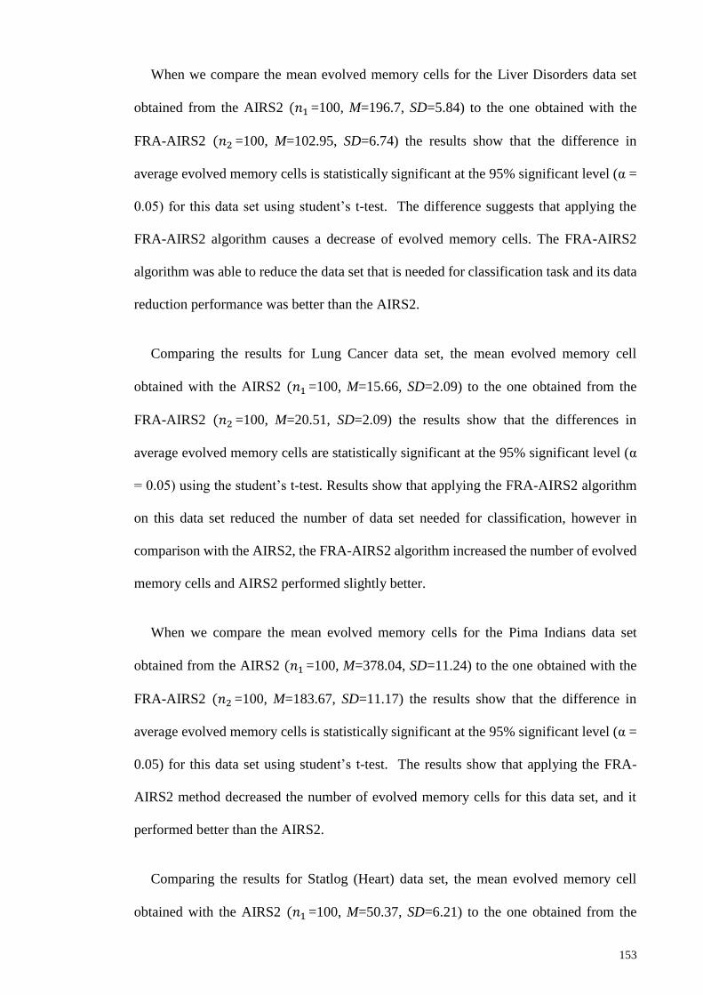
153
When we compare the mean evolved memory cells for the Liver Disorders data set
obtained from the AIRS2 (𝑛1 =100, M=196.7, SD=5.84) to the one obtained with the
FRA-AIRS2 (𝑛2 =100, M=102.95, SD=6.74) the results show that the difference in
average evolved memory cells is statistically significant at the 95% significant level (α =
0.05) for this data set using student’s t-test. The difference suggests that applying the
FRA-AIRS2 algorithm causes a decrease of evolved memory cells. The FRA-AIRS2
algorithm was able to reduce the data set that is needed for classification task and its data
reduction performance was better than the AIRS2.
Comparing the results for Lung Cancer data set, the mean evolved memory cell
obtained with the AIRS2 (𝑛1 =100, M=15.66, SD=2.09) to the one obtained from the
FRA-AIRS2 (𝑛2 =100, M=20.51, SD=2.09) the results show that the differences in
average evolved memory cells are statistically significant at the 95% significant level (α
= 0.05) using the student’s t-test. Results show that applying the FRA-AIRS2 algorithm
on this data set reduced the number of data set needed for classification, however in
comparison with the AIRS2, the FRA-AIRS2 algorithm increased the number of evolved
memory cells and AIRS2 performed slightly better.
When we compare the mean evolved memory cells for the Pima Indians data set
obtained from the AIRS2 (𝑛1 =100, M=378.04, SD=11.24) to the one obtained with the
FRA-AIRS2 (𝑛2 =100, M=183.67, SD=11.17) the results show that the difference in
average evolved memory cells is statistically significant at the 95% significant level (α =
0.05) for this data set using student’s t-test. The results show that applying the FRA-
AIRS2 method decreased the number of evolved memory cells for this data set, and it
performed better than the AIRS2.
Comparing the results for Statlog (Heart) data set, the mean evolved memory cell
obtained with the AIRS2 (𝑛1 =100, M=50.37, SD=6.21) to the one obtained from the

154
FRA-AIRS2 (𝑛2 =100, M=51.96, SD=6.02) the results show that the differences in
average evolved memory cells are statistically significant at the 95% significant level (α
= 0.05) using the student’s t-test. Results show that the FRA-AIRS2 algorithm decreased
the number of evolved memory cells for this data set and its data reduction capability was
better than that of the AIRS2.
When we compare the mean evolved memory cells for the Statlog (Image
Segmentation) data set obtained from the AIRS2 (𝑛1 =100, M=219.79, SD=11.71) to the
one obtained with the FRA-AIRS2 (𝑛2 =100, M=107.77, SD=7.81) the results show that
the difference in average evolved memory cells is statistically significant at the 95%
significant level (α = 0.05) for this data set using student’s t-test. The results show that
applying the FRA-AIRS2 algorithm decreased the number of evolved memory cells for
this data set, and it performed better than the AIRS2.
Comparing the results for the Statlog (Vehicle Silhouettes) data set, the mean evolved
memory cell obtained with the AIRS2 (𝑛1 =100, M=354.88, SD=12.30) to the one
obtained from the FRA-AIRS2 (𝑛2 =100, M=132.94, SD=7.89) the results show that the
differences in average evolved memory cells are statistically significant at the 95%
significant level (α = 0.05) using the student’s t-test. Results show that applying the FRA-
AIRS2 algorithm on this data set reduced the number of data set needed for classification,
and it performed better than the AIRS2.
When we compare the mean evolved memory cells for the Sonar data set obtained
from the AIRS2 (𝑛1 =100, M=143.33, SD=8.76) to the one obtained with the FRA-AIRS2
(𝑛2 =100, M=61.69, SD=5.83) the results show that the difference in average evolved
memory cells is statistically significant at the 95% significant level (α = 0.05) for this data
set using student’s t-test. The results show that applying the FRA-AIRS2 algorithm

155
decreased the number of evolved memory cells for this data set, and it performed better
than the AIRS2.
Comparing the results for the Vertebral Column_2C data set, the mean evolved
memory cell obtained with the AIRS2 (𝑛1 =100, M=151.75, SD=6.28) to the one obtained
from the FRA-AIRS2 (𝑛2 =100, M=102.32, SD=9.26) the results show that the
differences in average evolved memory cells are statistically significant at the 95%
significant level (α = 0.05) using the student’s t-test. Results show that applying the FRA-
AIRS2 algorithm on this data set reduced the number of data set needed for classification,
and it performed better than the AIRS2.
When we compare the mean evolved memory cells for the Vertebral Column_3C data
set obtained from the AIRS2 (𝑛1 =100, M=153.52, SD=6.43) to the one obtained with the
FRA-AIRS2 (𝑛2 =100, M=104.51, SD=8.34) the results show that the difference in
average evolved memory cells is statistically significant at the 95% significant level (α =
0.05) for this data set using student’s t-test. The results show that applying the FRA-
AIRS2 algorithm decreased the number of evolved memory cells for this data set, and it
performed better than the AIRS2.
Comparing the results for the Vertebral Wisconsin Breast Cancer Data Set (WBCD)
(Original) data set, the mean evolved memory cell obtained with the AIRS2 (𝑛1 =100,
M=227.82, SD=6.60) to the one obtained from the FRA-AIRS2 (𝑛2 =100, M=214.74,
SD=6.67) the results show that the differences in average evolved memory cells are
statistically significant at the 95% significant level (α = 0.05) using the student’s t-test.
Results show that applying the FRA-AIRS2 algorithm on this data set reduced the number
of data set needed for classification, and it performed better than the AIRS2.
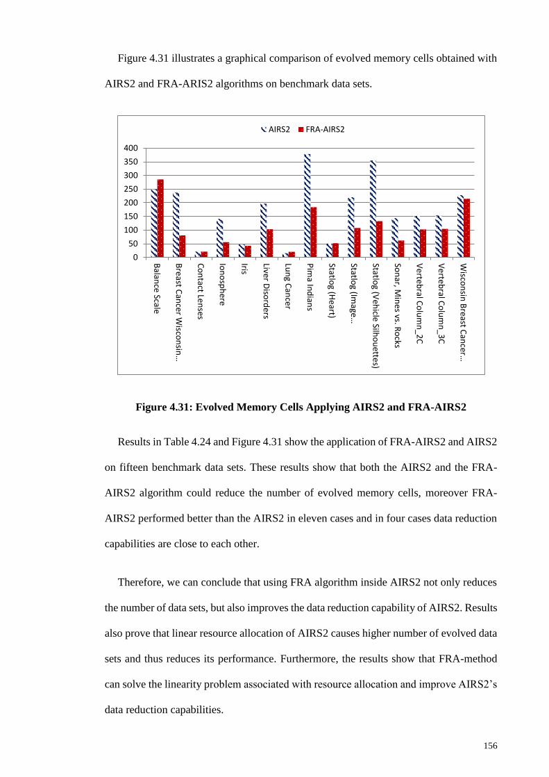
156
Figure 4.31 illustrates a graphical comparison of evolved memory cells obtained with
AIRS2 and FRA-ARIS2 algorithms on benchmark data sets.
Figure 4.31: Evolved Memory Cells Applying AIRS2 and FRA-AIRS2
Results in Table 4.24 and Figure 4.31 show the application of FRA-AIRS2 and AIRS2
on fifteen benchmark data sets. These results show that both the AIRS2 and the FRA-
AIRS2 algorithm could reduce the number of evolved memory cells, moreover FRA-
AIRS2 performed better than the AIRS2 in eleven cases and in four cases data reduction
capabilities are close to each other.
Therefore, we can conclude that using FRA algorithm inside AIRS2 not only reduces
the number of data sets, but also improves the data reduction capability of AIRS2. Results
also prove that linear resource allocation of AIRS2 causes higher number of evolved data
sets and thus reduces its performance. Furthermore, the results show that FRA-method
can solve the linearity problem associated with resource allocation and improve AIRS2’s
data reduction capabilities.
0
50
100
150
200
250
300
350
400
Balan
ce Scale
Bre
ast Can
cer W
iscon
sin…
Co
ntact Le
nses
Ion
osp
here
Iris
Liver Diso
rders
Lun
g Can
cer
Pim
a Ind
ians
Statlog (H
eart)
Statlog (Im
age…
Statlog (V
ehicle
Silho
uette
s)
Son
ar, Min
es vs. Ro
cks
Ve
rtebral C
olu
mn
_2C
Ve
rtebral C
olu
mn
_3C
Wisco
nsin
Breast C
ancer…
AIRS2 FRA-AIRS2

157
Comparison of Data Reduction Capabilities of FSR-AIRS2 and AIRS2
Figure 4.32 illustrates a graphical comparison of data reduction obtained with AIRS2
and FSR-ARIS2 on benchmark data sets.
Figure 4.32: Comparison of Data Reduction between AIRS2 and FSR-AIRS2
0
10
20
30
40
50
60
70
80
90
100
Balan
ce Scale
Bre
ast Can
cer W
iscon
sin (D
iagno
stic)
Co
ntact Le
nses
Ion
osp
here
Iris
Liver Diso
rders
Lun
g Can
cer
Pim
a Ind
ians
Statlog (H
eart)
Statlog (Im
age Segm
entatio
n)
Statlog (V
ehicle
Silho
uette
s)
Son
ar, Min
es vs. Ro
cks
Ve
rtebral C
olu
mn
_2C
Ve
rtebral C
olu
mn
_3C
Wisco
nsin
Breast C
ancer D
ata Set (W
BC
D) (O
riginal)
AIRS2 FSR-AIRS2

158
Table 4.25 presents total number of Instances for each data set, total evolved memory
cells through each algorithm and the percentage of data reduction achieved by AIRS2 and
FSR-AIRS2 on benchmark data sets.
Table 4.25: Comparison of Data Reduction Capabilities of FSR-AIRS2 and
AIRS2
AIRS2 FSR-AIRS2
Training set Total
Instances
Total
Memory
Cell
Data
Reduction
Percentage
Total
Memory
Cell
Data
Reduction
Percentage
Balance Scale 625 293 53.12% 428 31.52%
Breast Cancer
Wisconsin
(Diagnostic)
569 229 59.75% 90 84.18%
Contact Lenses 24 24 0.00% 24 0.00%
Ionosphere 351 148 57.84% 123 64.96%
Iris 150 48 68.00% 50 66.67%
Liver Disorders 345 208 39.71% 186 46.09%
Lung Cancer 32 31 3.13% 28 12.5%
Pima Indians 768 461 39.97% 357 53.52%
Statlog (Heart) 270 154 42.96% 137 49.26%
Statlog (Image
Segmentation)
2310 251 89.13% 93 95.97%
Statlog (Vehicle
Silhouettes)
846 368 56.50% 192 77.30%
Sonar, Mines vs.
Rocks
208 148 28.85% 98 52.89%
Vertebral
Column_2C
310 167 46.13% 160 48.39%
Vertebral
Column_3C
310 160 48.39% 145 53.23%
Wisconsin Breast
Cancer Data Set
(WBCD) (Original)
699 235 66.38% 237 84.18%
Equation (3.3) is used to calculate the data reduction percentage; it compares the
number of developed memory cells with the size of the training data sets. Results show
that both AIRS2 and FSR-AIRS2 can reduce the data sets that are required to perform the
classification tasks. The initial training records were used to create these reduced data
sets, which are evolved memory cells. Results indicate that FSR-AIRS2 shows greater
data reduction tendency than AIRS2. For most of the data sets the degree of data reduction

159
is greatly increased: from 59.75% to 84.18% for Breast Cancer Wisconsin (Diagnostic)
data, from 57.84% to 64.9% for Ionosphere data, from 39.71% to 46.09% for Liver
Disorders data, from 3.13% to 12.5% for Lung Cancer data, from 39.97% to 53.52% for
Pima Indians Diabetes data, from 42.96% to 49.26% for Statlog (Heart) data, from
89.13% to 95.97% for Statlog (Image Segmentation) data, from 56.5% to 77.3% for
Statlog (Vehicle Silhouettes) data, from 28.85% to 52.89% for Sonar data, from 46.13%
to 48.39% for Vertebral Column 2C data, from 48.39% to 53.23% for Vertebral Column
3C data, and from 66.38% to 84.18% for Wisconsin Breast Cancer Data Set (WBCD)
(Original) data. Since the total instance of Contact Lenses is 24, both AIRS2 and FSR-
AIRS2 could not perform classification with less than 24 instances, therefore the data
reduction percentage for both models are 0.00%. It should also be noted that with few
instances, there would not be enough records to perform the 10-fold cross validation.
Many real-world data sets are large in size and any algorithm that can reduce the volumes
of these data sets while maintaining the significant feature Using less of the data sets is
useful. data instances for classification tasks reduces also the classification time. As we
have seen in Table 4.8, FSR-AIRS2’ classification accuracy was higher than that of
AIRS2, this means that the proposed algorithm could reduce the volume of data sets
without sacrificing the classification accuracy. Although FSR-AIRS2 has shown greater
efficiency than AIRS2 without sacrificing accuracy, but it cannot be accepted blindly as
a feature of FSR-AIRS2. Of course, data reduction depends on the domain, and there can
be no assurance that FSR-AIRS2 would keep the trend for all data sets.
4.6.3.4 Comparing Running Time of FSR-AIRS2 with that of benchmark
algorithms
Table 4.26 illustrates the best average test set running time, together with the standard
deviations (given in parenthesis) obtained from FSR-AIRS2 and other well-known
classifiers: AIRS2, 1-KNN, 7-KNN, C4.5/J48, CLONALG, Immunos99, LibSVM,

160
Logistic, MLP, Naïve Bayes, RBF Network, SMO, and SMO2 on the Balance Scale data
sets. All experiments utilized 10 fold cross validation and were averaged over 10 runs.
Table 4.26: Running time measured in seconds [s] on Balance Scale Data Set
FSR-AIRS2 AIRS2 1KNN 7KNN C4.5/J48 CLONALG
0.016
(0.005)
0.111
(0.011)
0.0
(0.0)
0.0
(0.0)
0.012
(0.008)
0.070
(0.008)
Immunos99 LibSVM Logistic MLP NBayes RBF Netw.
0.127
(0.008)
0.041
(0.008)
0.020
(0.007)
0.487
(0.014)
0.0
(0.0)
0.027
(0.007)
SMO SMO2
0.020
(0.007)
0.096
(0.020)
Figure 4.33 illustrate a comparative graph of various classifiers’ running time on the
Balance Scale data sets. By looking at this Figure and Table 4.26 we can see that 1KNN,
7KNN, and NBayes are clear winners; they perform much better than other classifiers,
including FSR-AIRS2. However, FSR-AIRS2 performs better or is comparable with
other well-known classifiers.
Figure 4.33: Comparison of Balance Scale Running time Results
Table 4.27 illustrates the best average test set running time, together with the standard
deviations (given in parenthesis) obtained from FSR-AIRS2 and other well-known
0.00000
0.05000
0.10000
0.15000
0.20000
0.25000
0.30000
0.35000
0.40000
0.45000
0.50000
Ru
nn
ig T
ime
[s]
Classifiers

161
classifiers: AIRS2, 1-KNN, 7-KNN, C4.5/J48, CLONALG, Immunos99, LibSVM,
Logistic, MLP, Naïve Bayes, RBF Network, SMO, and SMO2 on the Breast Cancer
Wisconsin (Diagnostic) data sets.
All experiments utilized 10 fold cross validation and were averaged over 10 runs.
Table 4.27: Running time measured in seconds [s] on Breast Cancer Wisconsin
(Diagnostic) Data Set
FSR-AIRS2 AIRS2 1KNN 7KNN C4.5/J48 CLONALG
0.010
(0.012)
0.210
(0.016)
0.0
(0.0)
0.0
(0.0)
0.022
(0.011)
0.192
(0.01)
Immunos99 LibSVM Logistic MLP NBayes RBF Netw.
0.205
(0.012)
0.215
(0.050)
0.038
(0.009)
3.471
(0.032)
0.004
(0.009)
0.053
(0.016)
SMO SMO2
0.007
(0.008)
0.032
(0.006)
Figure 4.34 illustrate a comparative graph of various classifiers’ running time on the
Breast Cancer Wisconsin (Diagnostic) data sets.
By looking at this Figure and Table 4.27 we can see that 1KNN, 7KNN, and NBayes
are clear winners; they perform much better than other classifiers, including FSR-AIRS2.
However, FSR-AIRS2 performs better or is comparable with other well-known
classifiers.

162
Figure 4.34: Comparison of Breast Cancer Wisconsin (Diagnostic) Running time
Results
Table 4.28 illustrates the best average test set running time, together with the standard
deviations (given in parenthesis) obtained from FSR-AIRS2 and other well-known
classifiers: AIRS2, 1-KNN, 7-KNN, C4.5/J48, CLONALG, Immunos99, LibSVM,
Logistic, MLP, Naïve Bayes, RBF Network, SMO, and SMO2 on the Contact Lenses
data sets. All experiments utilized 10 fold cross validation and were averaged over 10
runs.
Table 4.28: Running time measured in seconds [s] on Contact Lenses Data Set
FSR-AIRS2 AIRS2 1KNN 7KNN C4.5/J48 CLONALG
0.004
(0.007)
0.004
(0.007)
0.0
(0.0)
0.0
(0.0)
0.0
(0.0)
0.003
(0.006)
Immunos99 LibSVM Logistic MLP NBayes RBF Netw.
0.0
(0.0)
0.001
(0.004)
0.0
(0.0)
0.028
(0.007)
0.0
(0.0)
0.003
(0.006)
SMO SMO2
0.010
(0.008)
0.011
(0.007)
Figure 4.35 illustrate a comparative graph of various classifiers’ running time on the
Contact Lenses data sets. By looking at this Figure and Table 4.28 we can see that 1KNN,
7KNN, C4.5/J48, Immunos99, Logistic, and NBayes are clear winners; they perform
0.00000
0.50000
1.00000
1.50000
2.00000
2.50000
3.00000
3.50000
Ru
nn
ig T
ime
[s]
Classifiers

163
much better than other classifiers, including FSR-AIRS2. However, FSR-AIRS2
performs better or is comparable with other well-known classifiers.
Figure 4.35: Comparison of Contact Lenses Running time Results
Table 4.29 illustrates the best average test set running time, together with the standard
deviations (given in parenthesis) obtained from FSR-AIRS2 and other well-known
classifiers: AIRS2, 1-KNN, 7-KNN, C4.5/J48, CLONALG, Immunos99, LibSVM,
Logistic, MLP, Naïve Bayes, RBF Network, SMO, and SMO2 on the Ionosphere data
sets. All experiments utilized 10 fold cross validation and were averaged over 10 runs.
Table 4.29: Running time measured in seconds [s] on Ionosphere Data Set
FSR-AIRS2 AIRS2 1KNN 7KNN C4.5/J48 CLONALG
0.011
(0.008)
0.260
(0.033)
0.0
(0.0)
0.0
(0.0)
0.027
(0.007)
0.128
(0.009)
Immunos99 LibSVM Logistic MLP NBayes RBF Netw.
0.083
(0.007)
0.063
(0.007)
0.026
(0.008)
2.680
(0.026)
0.005
(0.008)
0.021
(0.008)
SMO SMO2
0.017
(0.004)
0.078
(0.017)
Figure 4.36 illustrate a comparative graph of various classifiers’ running time on the
Ionosphere data sets. By looking at this Figure and Table 4.29 we can see that 1KNN,
0.00000
0.00500
0.01000
0.01500
0.02000
0.02500
0.03000
Ru
nn
ig T
ime
[s]
Classifiers

164
7KNN, and NBayes are clear winners; they perform much better than other classifiers,
including FSR-AIRS2. However, FSR-AIRS2 performs better or is comparable with
other well-known classifiers.
Figure 4.36: Comparison of Ionosphere Running time Results
Table 4.30 illustrates the best average test set running time, together with the standard
deviations (given in parenthesis) obtained from FSR-AIRS2 and other well-known
classifiers: AIRS2, 1-KNN, 7-KNN, C4.5/J48, CLONALG, Immunos99, LibSVM,
Logistic, MLP, Naïve Bayes, RBF Network, SMO, and SMO2 on the Iris data sets. All
experiments utilized 10 fold cross validation and were averaged over 10 runs.
Table 4.30: Running time measured in seconds [s] on Iris Data Set
FSR-AIRS2 AIRS2 1KNN 7KNN C4.5/J48 CLONALG
0.001
(0.004)
0.014
(0.006)
0.0
(0.0)
0.0
(0.0)
0.0
(0.0)
0.018
(0.005)
Immunos99 LibSVM Logistic MLP NBayes RBF Netw.
0.005
(0.007)
0.005
(0.007)
0.007
(0.008)
0.200
(0.097)
0.001
(0.024)
0.009
(0.008)
SMO SMO2
0.010
(0.007)
0.012
(0.006)
0.00000
0.50000
1.00000
1.50000
2.00000
2.50000
3.00000R
un
nig
Tim
e [
s]
Classifiers

165
Figure 4.37 illustrate a comparative graph of various classifiers’ running time on the
Iris data sets. By looking at this Figure and Table 4.30 we can see that 1KNN, 7KNN,
and C4.5/J48 are clear winners; they perform much better than other classifiers, including
FSR-AIRS2. However, FSR-AIRS2 performs better or is comparable with other well-
known classifiers.
Figure 4.37: Comparison of Iris Running time Results
Table 4.31 illustrates the best average test set running time, together with the standard
deviations (given in parenthesis) obtained from FSR-AIRS2 and other well-known
classifiers: AIRS2, 1-KNN, 7-KNN, C4.5/J48, CLONALG, Immunos99, LibSVM,
Logistic, MLP, Naïve Bayes, RBF Network, SMO, and SMO2 on the Liver Disorders
data sets. All experiments utilized 10 fold cross validation and were averaged over 10
runs.
Table 4.31: Running time measured in seconds [s] on Liver Disorders Data Set
FSR-AIRS2 AIRS2 1KNN 7KNN C4.5/J48 CLONALG
0.007
(0.008)
0.062
(0.031)
0.0
(0.0)
0.0
(0.0)
0.005
(0.007)
0.042
(0.008)
Immunos99 LibSVM Logistic MLP NBayes RBF Netw.
0.042
(0.007)
0.029
(0.308)
0.004
(0.007)
0.085
(0.008)
0.0
(0.0)
0.008
(0.008)
SMO SMO2
0.005
(0.007)
0.046
(0.014)
0.00000
0.05000
0.10000
0.15000
0.20000
Ru
nn
ig T
ime
[s]
Cassifiers

166
Figure 4.38 illustrate a comparative graph of various classifiers’ running time on the
Liver Disorders data sets. By looking at this Figure and Table 4.31 we can see that 1KNN,
7KNN, and NBayes are clear winners; they perform much better than other classifiers,
including FSR-AIRS2. However, FSR-AIRS2 performs better or is comparable with
other well-known classifiers.
Figure 4.38: Comparison of Liver Disorders Running time Results
Table 4.32 illustrates the best average test set running time, together with the standard
deviations (given in parenthesis) obtained from FSR-AIRS2 and other well-known
classifiers: AIRS2, 1-KNN, 7-KNN, C4.5/J48, CLONALG, Immunos99, LibSVM,
Logistic, MLP, Naïve Bayes, RBF Network, SMO, and SMO2 on the Lung Cancer data
sets. All experiments utilized 10 fold cross validation and were averaged over 10 runs.
Table 4.32: Running time measured in seconds [s] on Lung Cancer Data Set
FSR-AIRS2 AIRS2 1KNN 7KNN C4.5/J48 CLONALG
0.004
(0.007)
0.002
(0.005)
0.0
(0.0)
0.0
(0.0)
0.002
(0.005)
0.019
(0.007)
Immunos99 LibSVM Logistic MLP NBayes RBF Netw.
0.001
(0.004)
0.004
(0.007)
0.018
(0.009)
0.054
(0.009)
0.0
(0.0)
0.006
(0.008)
SMO SMO2
0.011
(0.007)
0.012
(0.007)
0.000000.010000.020000.030000.040000.050000.060000.070000.080000.09000
Ru
nn
ig T
ime
[s]
Classifiers
167
Figure 4.39 illustrate a comparative graph of various classifiers’ running time on the
Lung Cancer data sets. By looking at this Figure and Table 4.32 we can see that 1KNN,
7KNN, and NBayes are clear winners; they perform much better than other classifiers,
including FSR-AIRS2. However, FSR-AIRS2 performs better or is comparable with
other well-known classifiers.
Figure 4.39: Comparison of Lung Cancer Running time Results
Table 4.33 illustrates the best average test set running time, together with the standard
deviations (given in parenthesis) obtained from FSR-AIRS2 and other well-known
classifiers: AIRS2, 1-KNN, 7-KNN, C4.5/J48, CLONALG, Immunos99, LibSVM,
Logistic, MLP, Naïve Bayes, RBF Network, SMO, and SMO2 on the Pima Indians data
sets. All experiments utilized 10 fold cross validation and were averaged over 10 runs.
Table 4.33: Running time measured in seconds [s] on Pima Indians Data Set
FSR-AIRS2 AIRS2 1KNN 7KNN C4.5/J48 CLONALG
0.026
(0.010)
0.130
(0.040)
0.0
(0.0)
0.0
(0.0)
0.009
(0.008)
0.113
(0.010)
Immunos99 LibSVM Logistic MLP NBayes RBF Netw.
0.239
(0.012)
0.125
(0.009)
0.011
(0.007)
0.100
(0.030)
0.002
(0.008)
0.020
(0.008)
SMO SMO2
0.011
(0.008)
0.185
(0.029)
0.00000
0.01000
0.02000
0.03000
0.04000
0.05000
0.06000
Ru
nn
ig T
ime
[s]
Classifiers

168
Figure 4.40 illustrate a comparative graph of various classifiers’ running time on the
Pima Indians data sets. By looking at this Figure and Table 4.33 we can see that 1KNN,
and 7KNN are clear winners; they perform much better than other classifiers, including
FSR-AIRS2. However, FSR-AIRS2 performs better or is comparable with other well-
known classifiers.
Figure 4.40: Comparison of Pima Indians Running time Results
Table 4.34 illustrates the best average test set running time, together with the standard
deviations (given in parenthesis) obtained from FSR-AIRS2 and other well-known
classifiers: AIRS2, 1-KNN, 7-KNN, C4.5/J48, CLONALG, Immunos99, LibSVM,
Logistic, MLP, Naïve Bayes, RBF Network, SMO, and SMO2 on the Statlog (Heart) data
sets. All experiments utilized 10 fold cross validation and were averaged over 10 runs.
Table 4.34: Running time measured in seconds [s] on Statlog (Heart) Data Set
FSR-AIRS2 AIRS2 1KNN 7KNN C4.5/J48 CLONALG
0.026
(0.013)
0.028
(0.021)
0.0
(0.0)
0.0
(0.0)
0.005
(0.007)
0.050
(0.009)
Immunos99 LibSVM Logistic MLP NBayes RBF Netw.
0.031
(0.004)
0.036
(0.008)
0.005
(0.007)
0.097
(0.009)
0.0
(0.0)
0.007
(0.008)
SMO SMO2
0.008
(0.008)
0.032
(0.008)
0.000000.100000.200000.300000.400000.500000.600000.700000.800000.900001.00000
Ru
nn
ig T
ime
[s]
Classifiers

169
Figure 4.41 illustrate a comparative graph of various classifiers’ running time on the
Statlog (Heart) data sets.
By looking at this Figure and Table 4.34 we can see that 1KNN, 7KNN, and NBayes
are clear winners; they perform much better than other classifiers, including FSR-AIRS2.
However, FSR-AIRS2 performs better or is comparable with other well-known
classifiers.
Figure 4.41: Comparison of Statlog (Heart) Running time Results
Table 4.35 illustrates the best average test set running time, together with the standard
deviations (given in parenthesis) obtained from FSR-AIRS2 and other well-known
classifiers: AIRS2, 1-KNN, 7-KNN, C4.5/J48, CLONALG, Immunos99, LibSVM,
Logistic, MLP, Naïve Bayes, RBF Network, SMO, and SMO2 on the Statlog (Image
Segmentation) data sets.
All experiments utilized 10 fold cross validation and were averaged over 10 runs.
0.00000
0.01000
0.02000
0.03000
0.04000
0.05000
0.06000
0.07000
0.08000
0.09000
0.10000
Ru
nn
ig T
ime
[s]
Classifiers

170
Table 4.35: Running time measured in seconds [s] on Statlog (Image
Segmentation) Data Set
FSR-AIRS2 AIRS2 1KNN 7KNN C4.5/J48 CLONALG
0.012
(0.007)
1.320
(0.080)
0.0
(0.0)
0.0
(0.0)
0.118
(0.010)
0.560
(0.015)
Immunos99 LibSVM Logistic MLP NBayes RBF Netw.
2.750
(0.027)
3.191
(0.308)
10.000
(0.017)
12.390
(0.100)
0.0
(0.0)
4.034
(1.350)
SMO SMO2
0.164
(0.010)
0.590
(0.034)
Figure 4.42 illustrate a comparative graph of various classifiers’ running time on the
Statlog (Image Segmentation) data sets. By looking at this Figure and Table 4.35 we can
see that 1KNN, 7KNN, and NBayes are clear winners; they perform much better than
other classifiers, including FSR-AIRS2. However, FSR-AIRS2 performs better or is
comparable with other well-known classifiers.
Figure 4.42: Comparison of Statlog (Image Segmentation) Running time Results
Table 4.36 illustrates the best average test set running time, together with the standard
deviations (given in parenthesis) obtained from FSR-AIRS2 and other well-known
classifiers: AIRS2, 1-KNN, 7-KNN, C4.5/J48, CLONALG, Immunos99, LibSVM,
Logistic, MLP, Naïve Bayes, RBF Network, SMO, and SMO2 on the Statlog (Vehicle
0.00000
2.00000
4.00000
6.00000
8.00000
10.00000
12.00000
14.00000
Ru
nn
ig T
ime
[s]
Classifiers

171
Silhouettes) data sets. All experiments utilized 10 fold cross validation and were averaged
over 10 runs.
Table 4.36: Running time measured in seconds [s] on Statlog (Vehicle
Silhouettes) Data Set
FSR-AIRS2 AIRS2 1KNN 7KNN C4.5/J48 CLONALG
0.014
(0.004)
0.221
(0.030)
0.0
(0.0)
0.0
(0.0)
0.030
(0.007)
0.187
(0.008)
Immunos99 LibSVM Logistic MLP NBayes RBF Netw.
0.343
(0.012)
0.472
(0.041)
0.284
(0.074)
4.428
(0.098)
0.003
(0.006)
0.155
(0.030)
SMO SMO2
0.066
(0.007)
0.323
(0.022)
Figure 4.43 illustrate a comparative graph of various classifiers’ running time on the
Statlog (Vehicle Silhouettes) data sets. By looking at this Figure and Table 4.36 we can
see that 1KNN, 7KNN, and NBayes are clear winners; they perform much better than
other classifiers, including FSR-AIRS2. However, FSR-AIRS2 performs better or is
comparable with other well-known classifiers.
Figure 4.43: Comparison of Statlog (Vehicle Silhouettes) Running time Results
Table 4.37 illustrates the best average test set running time, together with the standard
deviations (given in parenthesis) obtained from FSR-AIRS2 and other well-known
0.00000
0.50000
1.00000
1.50000
2.00000
2.50000
3.00000
3.50000
4.00000
4.50000
Ru
nn
ig T
ime
[s]
Classifiers
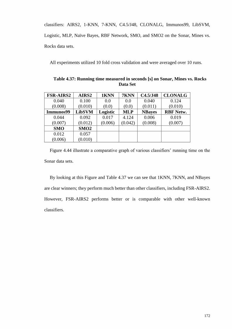
172
classifiers: AIRS2, 1-KNN, 7-KNN, C4.5/J48, CLONALG, Immunos99, LibSVM,
Logistic, MLP, Naïve Bayes, RBF Network, SMO, and SMO2 on the Sonar, Mines vs.
Rocks data sets.
All experiments utilized 10 fold cross validation and were averaged over 10 runs.
Table 4.37: Running time measured in seconds [s] on Sonar, Mines vs. Rocks
Data Set
FSR-AIRS2 AIRS2 1KNN 7KNN C4.5/J48 CLONALG
0.040
(0.008)
0.100
(0.010)
0.0
(0.0)
0.0
(0.0)
0.040
(0.011)
0.124
(0.010)
Immunos99 LibSVM Logistic MLP NBayes RBF Netw.
0.044
(0.007)
0.092
(0.012)
0.017
(0.006)
4.124
(0.042)
0.006
(0.008)
0.019
(0.007)
SMO SMO2
0.012
(0.006)
0.057
(0.010)
Figure 4.44 illustrate a comparative graph of various classifiers’ running time on the
Sonar data sets.
By looking at this Figure and Table 4.37 we can see that 1KNN, 7KNN, and NBayes
are clear winners; they perform much better than other classifiers, including FSR-AIRS2.
However, FSR-AIRS2 performs better or is comparable with other well-known
classifiers.
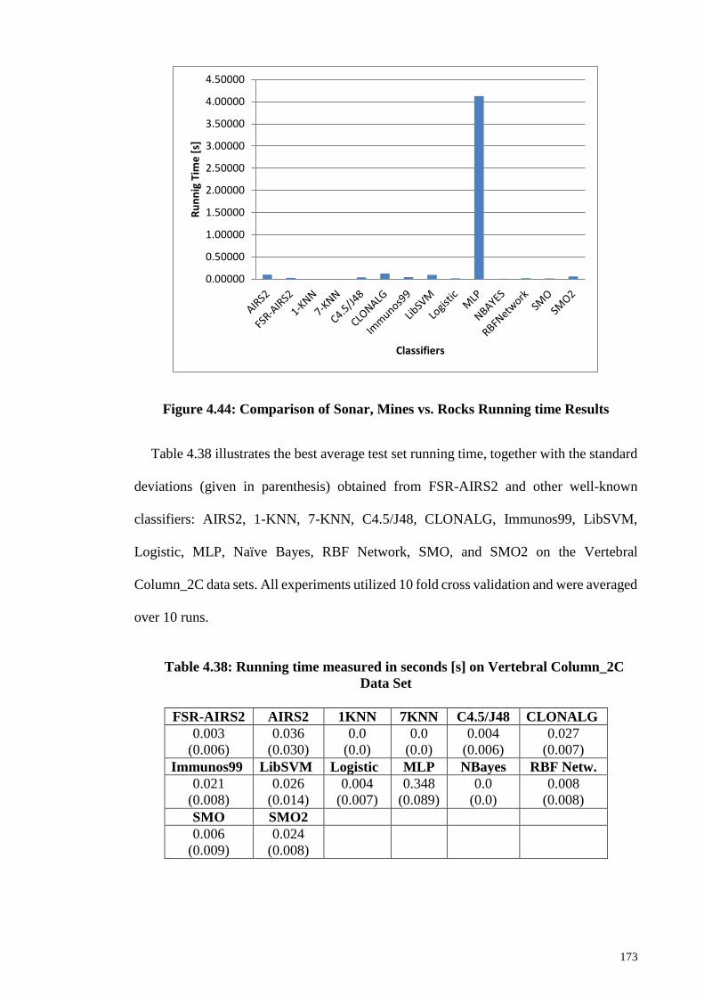
173
Figure 4.44: Comparison of Sonar, Mines vs. Rocks Running time Results
Table 4.38 illustrates the best average test set running time, together with the standard
deviations (given in parenthesis) obtained from FSR-AIRS2 and other well-known
classifiers: AIRS2, 1-KNN, 7-KNN, C4.5/J48, CLONALG, Immunos99, LibSVM,
Logistic, MLP, Naïve Bayes, RBF Network, SMO, and SMO2 on the Vertebral
Column_2C data sets. All experiments utilized 10 fold cross validation and were averaged
over 10 runs.
Table 4.38: Running time measured in seconds [s] on Vertebral Column_2C
Data Set
FSR-AIRS2 AIRS2 1KNN 7KNN C4.5/J48 CLONALG
0.003
(0.006)
0.036
(0.030)
0.0
(0.0)
0.0
(0.0)
0.004
(0.006)
0.027
(0.007)
Immunos99 LibSVM Logistic MLP NBayes RBF Netw.
0.021
(0.008)
0.026
(0.014)
0.004
(0.007)
0.348
(0.089)
0.0
(0.0)
0.008
(0.008)
SMO SMO2
0.006
(0.009)
0.024
(0.008)
0.00000
0.50000
1.00000
1.50000
2.00000
2.50000
3.00000
3.50000
4.00000
4.50000
Ru
nn
ig T
ime
[s]
Classifiers

174
Figure 4.45 illustrate a comparative graph of various classifiers’ running time on the
Vertebral Column_2C data sets.
By looking at this Figure and Table 4.38 we can see that 1KNN, 7KNN, and NBayes
are clear winners; they perform much better than other classifiers, including FSR-AIRS2.
However, FSR-AIRS2 performs better or is comparable with other well-known
classifiers.
Figure 4.45: Comparison of Vertebral Column_2C Running time Results
Table 4.39 illustrates the best average test set running time, together with the standard
deviations (given in parenthesis) obtained from FSR-AIRS2 and other well-known
classifiers: AIRS2, 1-KNN, 7-KNN, C4.5/J48, CLONALG, Immunos99, LibSVM,
Logistic, MLP, Naïve Bayes, RBF Network, SMO, and SMO2 on the Vertebral
Column_3C data sets.
All experiments utilized 10 fold cross validation and were averaged over 10 runs.
0.00000
0.05000
0.10000
0.15000
0.20000
0.25000
0.30000
0.35000
Ru
nn
ig T
ime
[s]
Classifiers

175
Table 4.39: Running time measured in seconds [s] on Vertebral Column_3C
Data Set
FSR-AIRS2 AIRS2 1KNN 7KNN C4.5/J48 CLONALG
0.003
(0.006)
0.029
(0.007)
0.0
(0.0)
0.0
(0.0)
0.005
(0.007)
0.028
(0.010)
Immunos99 LibSVM Logistic MLP NBayes RBF Netw.
0.019
(0.006)
0.033
(0.006)
0.010
(0.010)
0.394
(0.014)
0.0
(0.0)
0.021
(0.009)
SMO SMO2
0.012
(0.007)
0.030
(0.009)
Figure 4.46 illustrate a comparative graph of various classifiers’ running time on the
Vertebral Column_3C data sets. By looking at this Figure and Table 4.39 we can see that
1KNN, 7KNN, and NBayes are clear winners; they perform much better than other
classifiers, including FSR-AIRS2. However, FSR-AIRS2 performs better or is
comparable with other well-known classifiers.
Figure 4.46: Comparison of Vertebral Column_3C Running time Results
Table 4.40 illustrates the best average test set running time, together with the standard
deviations (given in parenthesis) obtained from FSR-AIRS2 and other well-known
classifiers: AIRS2, 1-KNN, 7-KNN, C4.5/J48, CLONALG, Immunos99, LibSVM,
Logistic, MLP, Naïve Bayes, RBF Network, SMO, and SMO2 on the Wisconsin Breast
0.00000
0.05000
0.10000
0.15000
0.20000
0.25000
0.30000
0.35000
0.40000
Ru
nn
ig T
ime
[s]
Classifiers

176
Cancer Data set (WBCD) (Original). All experiments utilized 10 fold cross validation and
were averaged over 10 runs.
Table 4.40: Running time measured in seconds [s] on Wisconsin Breast Cancer
Data Set (WBCD) Original
FSR-AIRS2 AIRS2 1KNN 7KNN C4.5/J48 CLONALG
0.015
(0.008)
0.141
(0.028)
0.0
(0.0)
0.0
(0.0)
0.007
(0.010)
0.11
(0.007)
Immunos99 LibSVM Logistic MLP NBayes RBF Netw.
0.186
(0.007)
0.110
(0.023)
0.020
(0.009)
1.177
(0.077)
0.003
(0.007)
0.029
(0.012)
SMO SMO2
0.007
(0.008)
0.039
(0.009)
Figure 4.47 illustrate a comparative graph of various classifiers’ running time on the
Wisconsin Breast Cancer Data Set (WBCD) (Original). By looking at this Figure and
Table 4.40 we can see that 1KNN, 7KNN, and NBayes are clear winners; they perform
much better than other classifiers, including FSR-AIRS2. However, FSR-AIRS2
performs better or is comparable with other well-known classifiers.
Figure 4.47: Comparison of Wisconsin Breast Cancer Data Set (WBCD) (Original)
Running time Results
0.00000
0.20000
0.40000
0.60000
0.80000
1.00000
1.20000
Ru
nn
ig T
ime
[s]
Classifiers
177
The results show some interesting patterns. While 1-KNN and 7-KNN are the clear
winner in terms of running time among all used classifiers, the running time of FSR-
AIRS2 was on 12 benchmark data sets lower, thus better than that of AIRS2, there was
one case where both of them were tie, and in 2 cases AIRS2 time was better than FSR-
AIRS2. In average, the running time of FSR-AIRS2 and C4.5/J48 were tie, while FSR-
AIRS2 performed faster than C4.5/J48 on 7 benchmark data sets, C4.5/J48 performed on
other 7 bench mark data sets faster and in only on one data set they were equal. The
running time of FSRARIS2 was lower than that of CLONALAG, MLP and SMO2 on all
benchmark data sets. Comparison between FSR-AIRS2 and Immunos99, LibSVM, RBF
Network, and SMO showed that in most cases, FSRARIS2 performed faster in the
running time. However, the running time of Naïve Bayes was in most cases lower than
FSR-AIRS2, only in one case FSR-AIRS2 performed faster.
While 3 classifiers performed faster in running time, FSR-AIRS2 was able to be faster
in most cases on the same benchmark data sets. This is of course encouraging, because it
shows that new implementations made in FSR-AIRS2 did not negatively affect the
running time of the classifier. The results suggest that FSR-AIRS2 is comparable to other
classifiers based on the running time.
4.6.3.5 Area under the curve (AUC)
Table 4.41 presents the best average test set of the area under ROC, together with the
standard deviations (given in parenthesis) obtained from FSR-AIRS2 and other well-
known classifiers: AIRS2, 1-KNN, 7-KNN, C4.5/J48, CLONALG, Immunos99,
LibSVM, Logistic, MLP, Naïve Bayes, RBF Network, SMO, and SMO2 on the Balance
Scale data sets. All experiments utilized 10 fold cross validation and were averaged over
10 runs.

178
Table 4.41: Comparison of FSR-AIRS2 and Other Classifiers' Area under ROC
on Balance Scale Data Set
FSR-AIRS2 AIRS2 1KNN 7KNN C4.5/J48 CLONALG
0.981
(0.023)
0.913
(0.034)
0.978
(0.010)
0.990
(0.006)
0.845
(0.041)
0.823
(0.054)
Immunos99 LibSVM Logistic MLP NBayes RBF Netw.
0.814
(0.062)
0.941
(0.024)
0.981
(0.011)
0.987
(0.014)
0.993
(0.007)
0.971
(0.020)
SMO SMO2
0.926
(0.024)
0.959
(0.019)
Figure 4.48 illustrate a comparative graph of various classifiers’ AUC on the Balance
Scale data sets. For interpretation of the values of area under the curve, this thesis uses
the grading point system that was discussed in section 3.4.6. By looking at Figure 4.48
and Table 4.41, we can see that AUCs of FSR-AIRS2 and ten other classifiers are above
0.9, which indicate that these classifiers perform excellent on this data set. The complete
interpretation is summarized in Table 4.56. The complete explanation is presented at the
end of this section, just after Figure 4.62 and before Table 4.56.
Figure 4.48: Comparison of FSR-AIRS2 and Other Classifiers' Area under ROC
on Balance Scale Data Sets
Table 4.42 presents the best average test set of the area under ROC, together with the
standard deviations (given in parenthesis) obtained from FSR-AIRS2 and other well-
0.00
0.10
0.20
0.30
0.40
0.50
0.60
0.70
0.80
0.90
1.00
AU
C
Classifiers

179
known classifiers: AIRS2, 1-KNN, 7-KNN, C4.5/J48, CLONALG, Immunos99,
LibSVM, Logistic, MLP, Naïve Bayes, RBF Network, SMO, and SMO2 on the Breast
Cancer Wisconsin (Diagnostic) data sets. All experiments utilized 10 fold cross validation
and were averaged over 10 runs.
Table 4.42: Comparison of FSR-AIRS2 and Other Classifiers' Area under ROC
on Breast Cancer Wisconsin (Diagnostic) Data Set
FSR-AIRS2 AIRS2 1KNN 7KNN C4.5/J48 CLONALG
1.000
(0.0)
0.955
(0.029)
0.953
(0.025)
0.990
(0.013)
0.927
(0.042)
0.869
(0.060)
Immunos99 LibSVM Logistic MLP NBayes RBF Netw.
0.840
(0.055)
0.500
(0.0)
0.973
(0.023)
0.992
(0.011)
0.981
(0.019)
0.981
(0.020)
SMO SMO2
0.969
(0.024)
0.975
(0.023)
Figure 4.49 illustrate a comparative graph of various classifiers’ AUC on the Breast
Cancer Wisconsin (Diagnostic) data sets. For interpretation of the values of area under
the curve, this thesis uses the grading point system that was discussed in section 3.4.6.
Figure 4.49: Comparison of FSR-AIRS2 and Other Classifiers' Area under ROC
on Breast Cancer Wisconsin (Diagnostic) Data Set
By looking at Figure 4.49 and Table 4.42, we can see that AUCs of FSR-AIRS2 and
ten other classifiers are above 0.9, which indicate that these classifiers perform excellent
0.000.100.200.300.400.500.600.700.800.901.00
AU
C
Classifiers
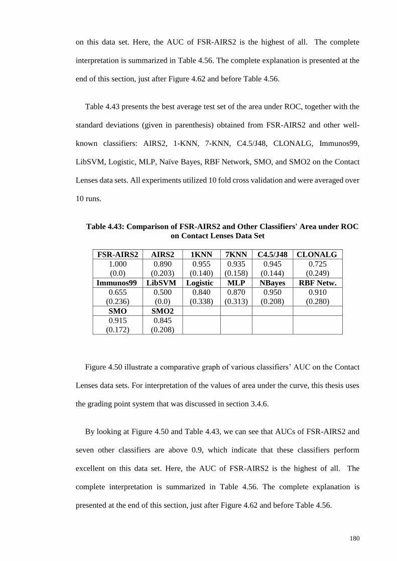
180
on this data set. Here, the AUC of FSR-AIRS2 is the highest of all. The complete
interpretation is summarized in Table 4.56. The complete explanation is presented at the
end of this section, just after Figure 4.62 and before Table 4.56.
Table 4.43 presents the best average test set of the area under ROC, together with the
standard deviations (given in parenthesis) obtained from FSR-AIRS2 and other well-
known classifiers: AIRS2, 1-KNN, 7-KNN, C4.5/J48, CLONALG, Immunos99,
LibSVM, Logistic, MLP, Naïve Bayes, RBF Network, SMO, and SMO2 on the Contact
Lenses data sets. All experiments utilized 10 fold cross validation and were averaged over
10 runs.
Table 4.43: Comparison of FSR-AIRS2 and Other Classifiers' Area under ROC
on Contact Lenses Data Set
FSR-AIRS2 AIRS2 1KNN 7KNN C4.5/J48 CLONALG
1.000
(0.0)
0.890
(0.203)
0.955
(0.140)
0.935
(0.158)
0.945
(0.144)
0.725
(0.249)
Immunos99 LibSVM Logistic MLP NBayes RBF Netw.
0.655
(0.236)
0.500
(0.0)
0.840
(0.338)
0.870
(0.313)
0.950
(0.208)
0.910
(0.280)
SMO SMO2
0.915
(0.172)
0.845
(0.208)
Figure 4.50 illustrate a comparative graph of various classifiers’ AUC on the Contact
Lenses data sets. For interpretation of the values of area under the curve, this thesis uses
the grading point system that was discussed in section 3.4.6.
By looking at Figure 4.50 and Table 4.43, we can see that AUCs of FSR-AIRS2 and
seven other classifiers are above 0.9, which indicate that these classifiers perform
excellent on this data set. Here, the AUC of FSR-AIRS2 is the highest of all. The
complete interpretation is summarized in Table 4.56. The complete explanation is
presented at the end of this section, just after Figure 4.62 and before Table 4.56.
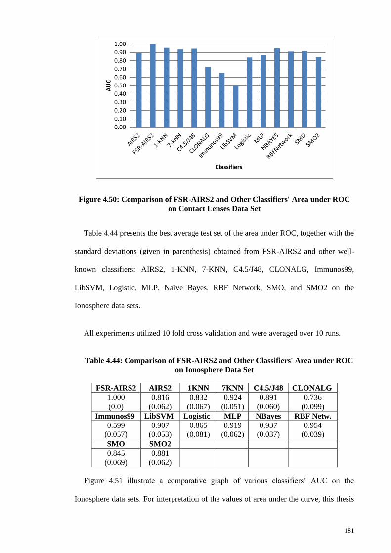
181
Figure 4.50: Comparison of FSR-AIRS2 and Other Classifiers' Area under ROC
on Contact Lenses Data Set
Table 4.44 presents the best average test set of the area under ROC, together with the
standard deviations (given in parenthesis) obtained from FSR-AIRS2 and other well-
known classifiers: AIRS2, 1-KNN, 7-KNN, C4.5/J48, CLONALG, Immunos99,
LibSVM, Logistic, MLP, Naïve Bayes, RBF Network, SMO, and SMO2 on the
Ionosphere data sets.
All experiments utilized 10 fold cross validation and were averaged over 10 runs.
Table 4.44: Comparison of FSR-AIRS2 and Other Classifiers' Area under ROC
on Ionosphere Data Set
FSR-AIRS2 AIRS2 1KNN 7KNN C4.5/J48 CLONALG
1.000
(0.0)
0.816
(0.062)
0.832
(0.067)
0.924
(0.051)
0.891
(0.060)
0.736
(0.099)
Immunos99 LibSVM Logistic MLP NBayes RBF Netw.
0.599
(0.057)
0.907
(0.053)
0.865
(0.081)
0.919
(0.062)
0.937
(0.037)
0.954
(0.039)
SMO SMO2
0.845
(0.069)
0.881
(0.062)
Figure 4.51 illustrate a comparative graph of various classifiers’ AUC on the
Ionosphere data sets. For interpretation of the values of area under the curve, this thesis
0.00
0.10
0.20
0.30
0.40
0.50
0.60
0.70
0.80
0.90
1.00
AU
C
Classifiers

182
uses the grading point system that was discussed in section 3.4.6. By looking at
Figure 4.51 and Table 4.44, we can see that AUCs of FSR-AIRS2 and six other classifiers
are above 0.9, which indicate that these classifiers perform excellent on this data set. Here,
the AUC of FSR-AIRS2 is the highest of all.
The complete interpretation is summarized in Table 4.56. The complete explanation is
presented at the end of this section, just after Figure 4.62 and before Table 4.56.
Figure 4.51: Comparison of FSR-AIRS2 and Other Classifiers' Area under ROC
on Ionosphere Data Set
Table 4.45 presents the best average test set of the area under ROC, together with the
standard deviations (given in parenthesis) obtained from FSR-AIRS2 and other well-
known classifiers: AIRS2, 1-KNN, 7-KNN, C4.5/J48, CLONALG, Immunos99,
LibSVM, Logistic, MLP, Naïve Bayes, RBF Network, SMO, and SMO2 on the Iris data
sets.
All experiments utilized 10 fold cross validation and were averaged over 10 runs.
0.000.100.200.300.400.500.600.700.800.901.00
AU
C
Classifiers

183
Table 4.45: Comparison of FSR-AIRS2 and Other Classifiers' Area under ROC
on Iris Data Set
FSR-AIRS2 AIRS2 1KNN 7KNN C4.5/J48 CLONALG
1.000
(0.0)
1.000
(0.0)
1.000
(0.0)
1.000
(0.0)
0.990
(0.030)
1.000
(0.0)
Immunos99 LibSVM Logistic MLP NBayes RBF Netw.
1.000
(0.0)
1.000
(0.0)
1.000
(0.0)
1.000
(0.0)
1.000
(0.0)
1.000
(0.0)
SMO SMO2
1.000
(0.0)
1.000
(0.0)
Figure 4.52 illustrate a comparative graph of various classifiers’ AUC on the Iris data
sets. For interpretation of the values of area under the curve, this thesis uses the grading
point system that was discussed in section 3.4.6. By looking at Figure 4.52 and Table 4.45,
we can see that AUCs of almost all classifiers equal 1.0, which indicate that these
classifiers perform excellent on this data set.
The complete interpretation is summarized in Table 4.56. The complete explanation is
presented at the end of this section, just after Figure 4.62 and before Table 4.56.
Figure 4.52: Comparison of FSR-AIRS2 and Other Classifiers' Area under ROC
on Iris Data Set
0.00
0.10
0.20
0.30
0.40
0.50
0.60
0.70
0.80
0.90
1.00
AU
C
Classifiers
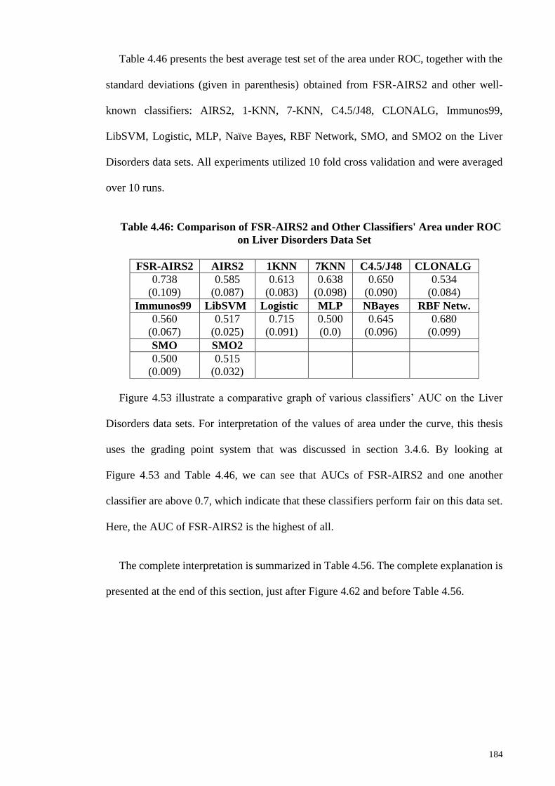
184
Table 4.46 presents the best average test set of the area under ROC, together with the
standard deviations (given in parenthesis) obtained from FSR-AIRS2 and other well-
known classifiers: AIRS2, 1-KNN, 7-KNN, C4.5/J48, CLONALG, Immunos99,
LibSVM, Logistic, MLP, Naïve Bayes, RBF Network, SMO, and SMO2 on the Liver
Disorders data sets. All experiments utilized 10 fold cross validation and were averaged
over 10 runs.
Table 4.46: Comparison of FSR-AIRS2 and Other Classifiers' Area under ROC
on Liver Disorders Data Set
FSR-AIRS2 AIRS2 1KNN 7KNN C4.5/J48 CLONALG
0.738
(0.109)
0.585
(0.087)
0.613
(0.083)
0.638
(0.098)
0.650
(0.090)
0.534
(0.084)
Immunos99 LibSVM Logistic MLP NBayes RBF Netw.
0.560
(0.067)
0.517
(0.025)
0.715
(0.091)
0.500
(0.0)
0.645
(0.096)
0.680
(0.099)
SMO SMO2
0.500
(0.009)
0.515
(0.032)
Figure 4.53 illustrate a comparative graph of various classifiers’ AUC on the Liver
Disorders data sets. For interpretation of the values of area under the curve, this thesis
uses the grading point system that was discussed in section 3.4.6. By looking at
Figure 4.53 and Table 4.46, we can see that AUCs of FSR-AIRS2 and one another
classifier are above 0.7, which indicate that these classifiers perform fair on this data set.
Here, the AUC of FSR-AIRS2 is the highest of all.
The complete interpretation is summarized in Table 4.56. The complete explanation is
presented at the end of this section, just after Figure 4.62 and before Table 4.56.

185
Figure 4.53: Comparison of FSR-AIRS2 and Other Classifiers' Area under ROC
on Liver Disorders Data Set
Table 4.47 presents the best average test set of the area under ROC, together with the
standard deviations (given in parenthesis) obtained from FSR-AIRS2 and other well-
known classifiers: AIRS2, 1-KNN, 7-KNN, C4.5/J48, CLONALG, Immunos99,
LibSVM, Logistic, MLP, Naïve Bayes, RBF Network, SMO, and SMO2 on the Lung
Cancer data sets.
All experiments utilized 10 fold cross validation and were averaged over 10 runs.
Table 4.47: Comparison of FSR-AIRS2 and Other Classifiers' Area under ROC
on Lung Cancer Data Set
FSR-AIRS2 AIRS2 1KNN 7KNN C4.5/J48 CLONALG
0.929
(0.176)
0.658
(0.284)
0.777
(0.252)
0.826
(0.224)
0.714
(0.256)
0.761
(0.260)
Immunos99 LibSVM Logistic MLP NBayes RBF Netw.
0.623
(0.272)
0.500
(0.0)
0.604
(0.428)
0.599
(0.295)
0.818
(0.254)
0.744
(0.312)
SMO SMO2
0.744
(0.271)
0.756
(0.281)
Figure 4.54 illustrate a comparative graph of various classifiers’ AUC on the Lung
Cancer data sets. For interpretation of the values of area under the curve, this thesis uses
0.00
0.10
0.20
0.30
0.40
0.50
0.60
0.70
0.80
0.90
1.00
AU
C
Classifiers
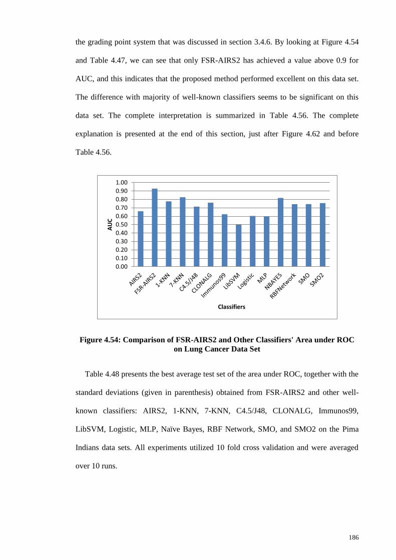
186
the grading point system that was discussed in section 3.4.6. By looking at Figure 4.54
and Table 4.47, we can see that only FSR-AIRS2 has achieved a value above 0.9 for
AUC, and this indicates that the proposed method performed excellent on this data set.
The difference with majority of well-known classifiers seems to be significant on this
data set. The complete interpretation is summarized in Table 4.56. The complete
explanation is presented at the end of this section, just after Figure 4.62 and before
Table 4.56.
Figure 4.54: Comparison of FSR-AIRS2 and Other Classifiers' Area under ROC
on Lung Cancer Data Set
Table 4.48 presents the best average test set of the area under ROC, together with the
standard deviations (given in parenthesis) obtained from FSR-AIRS2 and other well-
known classifiers: AIRS2, 1-KNN, 7-KNN, C4.5/J48, CLONALG, Immunos99,
LibSVM, Logistic, MLP, Naïve Bayes, RBF Network, SMO, and SMO2 on the Pima
Indians data sets. All experiments utilized 10 fold cross validation and were averaged
over 10 runs.
0.00
0.10
0.20
0.30
0.40
0.50
0.60
0.70
0.80
0.90
1.00
AU
C
Classifiers

187
Table 4.48: Comparison of FSR-AIRS2 and Other Classifiers' Area under ROC
on Pima Indians Data Set
FSR-AIRS2 AIRS2 1KNN 7KNN C4.5/J48 CLONALG
0.996
(0.015)
0.694
(0.062)
0.668
(0.051)
0.787
(0.053)
0.751
(0.069)
0.595
(0.073)
Immunos99 LibSVM Logistic MLP NBayes RBF Netw.
0.563
(0.056)
0.500
(0.0)
0.831
(0.049)
0.800
(0.054)
0.815
(0.051)
0.789
(0.056)
SMO SMO2
0.713
(0.055)
0.716
(0.055)
Figure 4.55 illustrate a comparative graph of various classifiers’ AUC on the Pima
Indians data sets. For interpretation of the values of area under the curve, this thesis uses
the grading point system that was discussed in section 3.4.6. By looking at Figure 4.55
and Table 4.48, we can see that only FSR-AIRS2 has achieved a value above 0.9 for
AUC, and this indicates that the proposed method performed excellent on this data set.
The difference with majority of well-known classifiers seems to be significant on this
data set.
The complete interpretation is summarized in Table 4.56. The complete explanation is
presented at the end of this section, just after Figure 4.62 and before Table 4.56.
Figure 4.55: Comparison of FSR-AIRS2 and Other Classifiers' Area under ROC
on Pima Indians Data Set
0.00
0.10
0.20
0.30
0.40
0.50
0.60
0.70
0.80
0.90
1.00
AU
C
Classifiers

188
Table 4.49 presents the best average test set of the area under ROC, together with the
standard deviations (given in parenthesis) obtained from FSR-AIRS2 and other well-
known classifiers: AIRS2, 1-KNN, 7-KNN, C4.5/J48, CLONALG, Immunos99,
LibSVM, Logistic, MLP, Naïve Bayes, RBF Network, SMO, and SMO2 on the Statlog
(Heart) data sets. All experiments utilized 10 fold cross validation and were averaged
over 10 runs.
Table 4.49: Comparison of FSR-AIRS2 and Other Classifiers' Area under ROC
on Statlog (Heart) Data Set
FSR-AIRS2 AIRS2 1KNN 7KNN C4.5/J48 CLONALG
0.846
(0.096)
0.770
(0.084)
0.760
(0.085)
0.873
(0.066)
0.786
(0.094)
0.623
(0.077)
Immunos99 LibSVM Logistic MLP NBayes RBF Netw.
0.653
(0.085)
0.504
(0.013)
0.905
(0.054)
0.500
(0.0)
0.902
(0.054)
0.891
(0.058)
SMO SMO2
0.834
(0.064)
0.808
(0.068)
Figure 4.56 illustrate a comparative graph of various classifiers’ AUC on the Statlog
(Heart) data sets. For interpretation of the values of area under the curve, this thesis uses
the grading point system that was discussed in section 3.4.6. By looking at Figure 4.56
and Table 4.49, we can see that Logistic and NBayes have achieved a value of 0.9 for
AUC, and this indicates that they performed excellent on this data set. FSR-AIRS2 ranked
5th and has got a grade of B (Good).
The complete interpretation is summarized in Table 4.56. The complete explanation is
presented at the end of this section, just after Figure 4.62 and before Table 4.56.
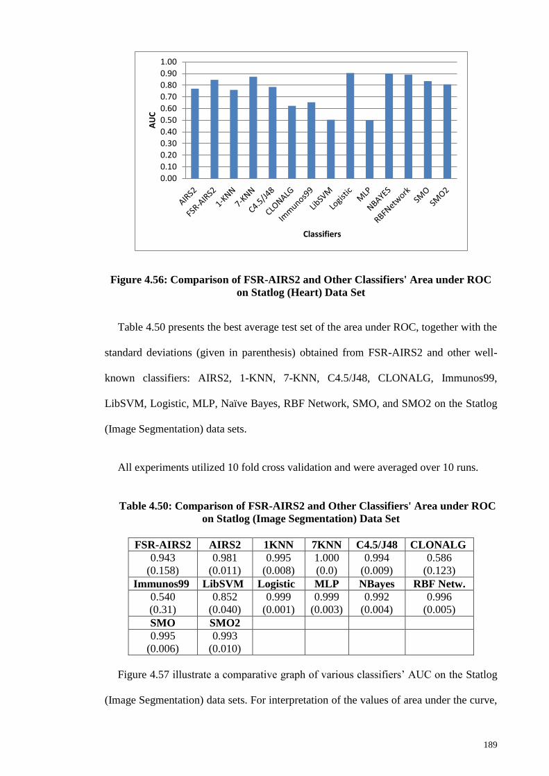
189
Figure 4.56: Comparison of FSR-AIRS2 and Other Classifiers' Area under ROC
on Statlog (Heart) Data Set
Table 4.50 presents the best average test set of the area under ROC, together with the
standard deviations (given in parenthesis) obtained from FSR-AIRS2 and other well-
known classifiers: AIRS2, 1-KNN, 7-KNN, C4.5/J48, CLONALG, Immunos99,
LibSVM, Logistic, MLP, Naïve Bayes, RBF Network, SMO, and SMO2 on the Statlog
(Image Segmentation) data sets.
All experiments utilized 10 fold cross validation and were averaged over 10 runs.
Table 4.50: Comparison of FSR-AIRS2 and Other Classifiers' Area under ROC
on Statlog (Image Segmentation) Data Set
FSR-AIRS2 AIRS2 1KNN 7KNN C4.5/J48 CLONALG
0.943
(0.158)
0.981
(0.011)
0.995
(0.008)
1.000
(0.0)
0.994
(0.009)
0.586
(0.123)
Immunos99 LibSVM Logistic MLP NBayes RBF Netw.
0.540
(0.31)
0.852
(0.040)
0.999
(0.001)
0.999
(0.003)
0.992
(0.004)
0.996
(0.005)
SMO SMO2
0.995
(0.006)
0.993
(0.010)
Figure 4.57 illustrate a comparative graph of various classifiers’ AUC on the Statlog
(Image Segmentation) data sets. For interpretation of the values of area under the curve,
0.00
0.10
0.20
0.30
0.40
0.50
0.60
0.70
0.80
0.90
1.00
AU
C
Classifiers

190
this thesis uses the grading point system that was discussed in section 3.4.6. By looking
at Figure 4.57 and Table 4.50, we can see that 7KNN, Logistic, and MLP, and RBF
Network have achieved a value very close to 1 for AUC. However, FSR-AIRS2 and ten
other well-known classifiers ranked excellent on this data set. The complete interpretation
is summarized in Table 4.56. The complete explanation is presented at the end of this
section, just after Figure 4.62 and before Table 4.56.
Figure 4.57: Comparison of FSR-AIRS2 and Other Classifiers' Area under ROC
on Statlog (Image Segmentation) Data Set
Table 4.51 presents the best average test set of the area under ROC, together with the
standard deviations (given in parenthesis) obtained from FSR-AIRS2 and other well-
known classifiers: AIRS2, 1-KNN, 7-KNN, C4.5/J48, CLONALG, Immunos99,
LibSVM, Logistic, MLP, Naïve Bayes, RBF Network, SMO, and SMO2 on the Statlog
(Vehicle Silhouettes) data sets.
All experiments utilized 10 fold cross validation and were averaged over 10 runs.
0.00
0.10
0.20
0.30
0.40
0.50
0.60
0.70
0.80
0.90
1.00
AU
C
Classifiers
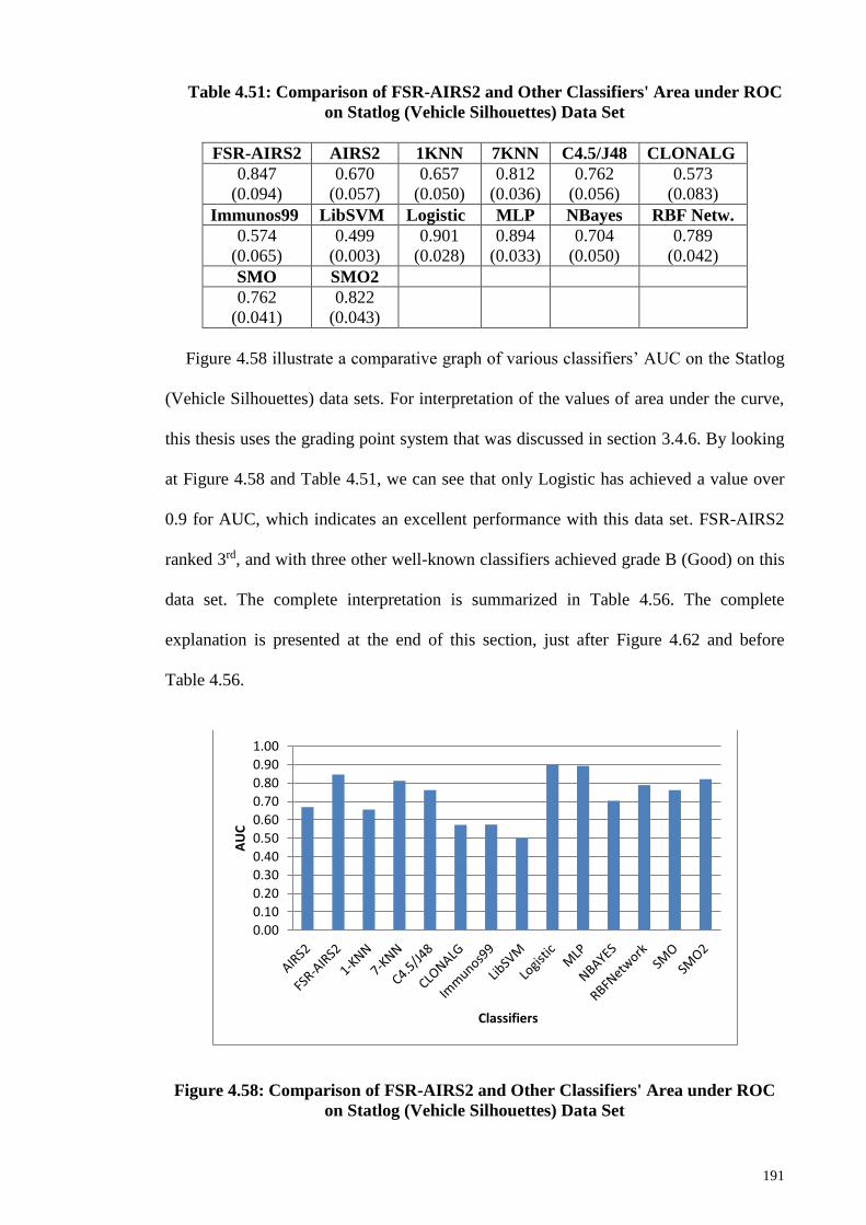
191
Table 4.51: Comparison of FSR-AIRS2 and Other Classifiers' Area under ROC
on Statlog (Vehicle Silhouettes) Data Set
FSR-AIRS2 AIRS2 1KNN 7KNN C4.5/J48 CLONALG
0.847
(0.094)
0.670
(0.057)
0.657
(0.050)
0.812
(0.036)
0.762
(0.056)
0.573
(0.083)
Immunos99 LibSVM Logistic MLP NBayes RBF Netw.
0.574
(0.065)
0.499
(0.003)
0.901
(0.028)
0.894
(0.033)
0.704
(0.050)
0.789
(0.042)
SMO SMO2
0.762
(0.041)
0.822
(0.043)
Figure 4.58 illustrate a comparative graph of various classifiers’ AUC on the Statlog
(Vehicle Silhouettes) data sets. For interpretation of the values of area under the curve,
this thesis uses the grading point system that was discussed in section 3.4.6. By looking
at Figure 4.58 and Table 4.51, we can see that only Logistic has achieved a value over
0.9 for AUC, which indicates an excellent performance with this data set. FSR-AIRS2
ranked 3rd, and with three other well-known classifiers achieved grade B (Good) on this
data set. The complete interpretation is summarized in Table 4.56. The complete
explanation is presented at the end of this section, just after Figure 4.62 and before
Table 4.56.
Figure 4.58: Comparison of FSR-AIRS2 and Other Classifiers' Area under ROC
on Statlog (Vehicle Silhouettes) Data Set
0.00
0.10
0.20
0.30
0.40
0.50
0.60
0.70
0.80
0.90
1.00
AU
C
Classifiers

192
Table 4.52 presents the best average test set of the area under ROC, together with the
standard deviations (given in parenthesis) obtained from FSR-AIRS2 and other well-
known classifiers: AIRS2, 1-KNN, 7-KNN, C4.5/J48, CLONALG, Immunos99,
LibSVM, Logistic, MLP, Naïve Bayes, RBF Network, SMO, and SMO2 on the Sonar,
Mines vs. Rocks data sets. All experiments utilized 10 fold cross validation and were
averaged over 10 runs.
Table 4.52: Comparison of FSR-AIRS2 and Other Classifiers' Area under ROC
on Sonar, Mines vs. Rocks Data Set
FSR-AIRS2 AIRS2 1KNN 7KNN C4.5/J48 CLONALG
0.979
(0.050)
0.662
(0.104)
0.859
(0.086)
0.890
(0.075)
0.753
(0.113)
0.632
(0.101)
Immunos99 LibSVM Logistic MLP NBayes RBF Netw.
0.603
(0.096)
0.629
(0.077)
0.762
(0.101)
0.887
(0.072)
0.800
(0.095)
0.812
(0.092)
SMO SMO2
0.764
(0.083)
0.835
(0.078)
Figure 4.59 illustrate a comparative graph of various classifiers’ AUC on the Sonar,
Mines vs. Rocks data sets. For interpretation of the values of area under the curve, this
thesis uses the grading point system that was discussed in section 3.4.6.
By looking at Figure 4.59 and Table 4.52, we can see that only FSR-AIRS2 has
achieved a value over 0.9 for AUC, which indicates an excellent performance with this
data set. Six of well-known classifiers achieved grade B (Good) on this data set.
The complete interpretation is summarized in Table 4.56. The complete explanation is
presented at the end of this section, just after Figure 4.62 and before Table 4.56.

193
Figure 4.59: Comparison of FSR-AIRS2 and Other Classifiers' Area under ROC
on Sonar, Mines vs. Rocks Data Set
Table 4.53 presents the best average test set of the area under ROC, together with the
standard deviations (given in parenthesis) obtained from FSR-AIRS2 and other well-
known classifiers: AIRS2, 1-KNN, 7-KNN, C4.5/J48, CLONALG, Immunos99,
LibSVM, Logistic, MLP, Naïve Bayes, RBF Network, SMO, and SMO2 on the Vertebral
Column_2C data sets. All experiments utilized 10 fold cross validation and were averaged
over 10 runs.
Table 4.53: Comparison of FSR-AIRS2 and Other Classifiers' Area under ROC
on Vertebral Column_2C Data Set
FSR-AIRS2 AIRS2 1KNN 7KNN C4.5/J48 CLONALG
0.842
(0.104)
0.730
(0.098)
0.801
(0.070)
0.851
(0.064)
0.843
(0.086)
0.695
(0.124)
Immunos99 LibSVM Logistic MLP NBayes RBF Netw.
0.793
(0.058)
0.500
(0.0)
0.936
(0.039)
0.930
(0.045)
0.881
(0.056)
0.881
(0.063)
SMO SMO2
0.709
(0.086)
0.714
(0.089)
Figure 4.60 illustrate a comparative graph of various classifiers’ AUC on the Vertebral
Column_2C data sets. For interpretation of the values of area under the curve, this thesis
uses the grading point system that was discussed in section 3.4.6. By looking at
0.00
0.10
0.20
0.30
0.40
0.50
0.60
0.70
0.80
0.90
1.00
AU
C
Classifiers

194
Figure 4.60 and Table 4.53, we can see that only Logistic and MLP have achieved a value
over 0.9 for AUC, which indicates an excellent performance with this data set. FSR-
AIRS2 ranked sixth, and together with five of well-known classifiers achieved grade B
(Good) on this data set.
The complete interpretation is summarized in Table 4.56. The complete explanation is
presented at the end of this section, just after Figure 4.62 and before Table 4.56.
Figure 4.60: Comparison of FSR-AIRS2 and Other Classifiers' Area under ROC
on Vertebral Column_2C Data Set
Table 4.54 presents the best average test set of the area under ROC, together with the
standard deviations (given in parenthesis) obtained from FSR-AIRS2 and other well-
known classifiers: AIRS2, 1-KNN, 7-KNN, C4.5/J48, CLONALG, Immunos99,
LibSVM, Logistic, MLP, Naïve Bayes, RBF Network, SMO, and SMO2 on the Vertebral
Column_3C data sets.
All experiments utilized 10 fold cross validation and were averaged over 10 runs.
0.00
0.10
0.20
0.30
0.40
0.50
0.60
0.70
0.80
0.90
1.00
AU
C
Classifiers

195
Table 4.54: Comparison of FSR-AIRS2 and Other Classifiers' Area under ROC
on Vertebral Column_3C Data Set
FSR-AIRS2 AIRS2 1KNN 7KNN C4.5/J48 CLONALG
0.890
(0.107)
0.739
(0.106)
0.747
(0.100)
0.890
(0.054)
0.839
(0.087)
0.656
(0.149)
Immunos99 LibSVM Logistic MLP NBayes RBF Netw.
0.752
(0.103)
0.500
(0.0)
0.947
(0.038)
0.940
(0.041)
0.925
(0.047)
0.909
(0.055)
SMO SMO2
0.833
(0.076)
0.852
(0.075)
Figure 4.61 illustrate a comparative graph of various classifiers’ AUC on the Vertebral
Column_3C data sets. For interpretation of the values of area under the curve, this thesis
uses the grading point system that was discussed in section 3.4.6. By looking at
Figure 4.61 and Table 4.54, we can see that Logistic, MLP, NBayes, and RBF Network
have achieved a value over 0.9 for AUC, which indicates an excellent performance with
this data set. FSR-AIRS2 ranked fifth, and together with four of well-known classifiers
achieved grade B (Good) on this data set.
The complete interpretation is summarized in Table 4.56. The complete explanation is
presented at the end of this section, just after Figure 4.62 and before Table 4.56.
Figure 4.61: Comparison of FSR-AIRS2 and Other Classifiers' Area under ROC
on Vertebral Column_3C Data Set
0.00
0.10
0.20
0.30
0.40
0.50
0.60
0.70
0.80
0.90
1.00
AU
C
Classifiers
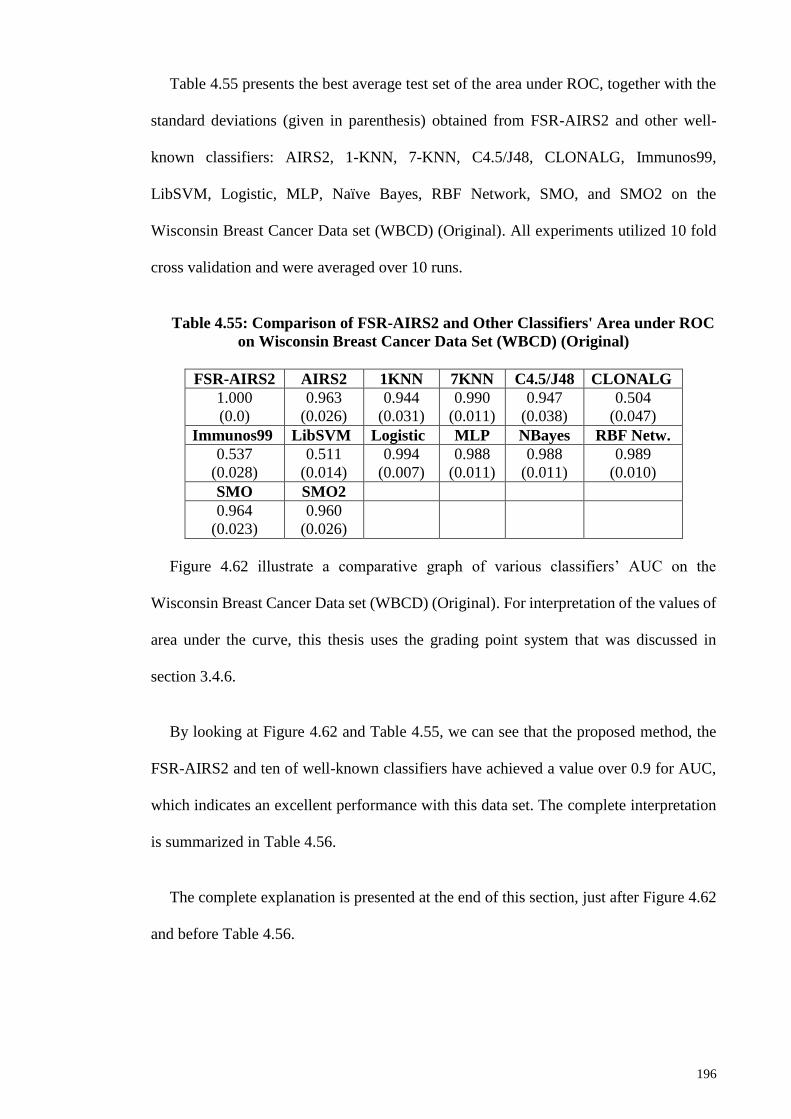
196
Table 4.55 presents the best average test set of the area under ROC, together with the
standard deviations (given in parenthesis) obtained from FSR-AIRS2 and other well-
known classifiers: AIRS2, 1-KNN, 7-KNN, C4.5/J48, CLONALG, Immunos99,
LibSVM, Logistic, MLP, Naïve Bayes, RBF Network, SMO, and SMO2 on the
Wisconsin Breast Cancer Data set (WBCD) (Original). All experiments utilized 10 fold
cross validation and were averaged over 10 runs.
Table 4.55: Comparison of FSR-AIRS2 and Other Classifiers' Area under ROC
on Wisconsin Breast Cancer Data Set (WBCD) (Original)
FSR-AIRS2 AIRS2 1KNN 7KNN C4.5/J48 CLONALG
1.000
(0.0)
0.963
(0.026)
0.944
(0.031)
0.990
(0.011)
0.947
(0.038)
0.504
(0.047)
Immunos99 LibSVM Logistic MLP NBayes RBF Netw.
0.537
(0.028)
0.511
(0.014)
0.994
(0.007)
0.988
(0.011)
0.988
(0.011)
0.989
(0.010)
SMO SMO2
0.964
(0.023)
0.960
(0.026)
Figure 4.62 illustrate a comparative graph of various classifiers’ AUC on the
Wisconsin Breast Cancer Data set (WBCD) (Original). For interpretation of the values of
area under the curve, this thesis uses the grading point system that was discussed in
section 3.4.6.
By looking at Figure 4.62 and Table 4.55, we can see that the proposed method, the
FSR-AIRS2 and ten of well-known classifiers have achieved a value over 0.9 for AUC,
which indicates an excellent performance with this data set. The complete interpretation
is summarized in Table 4.56.
The complete explanation is presented at the end of this section, just after Figure 4.62
and before Table 4.56.
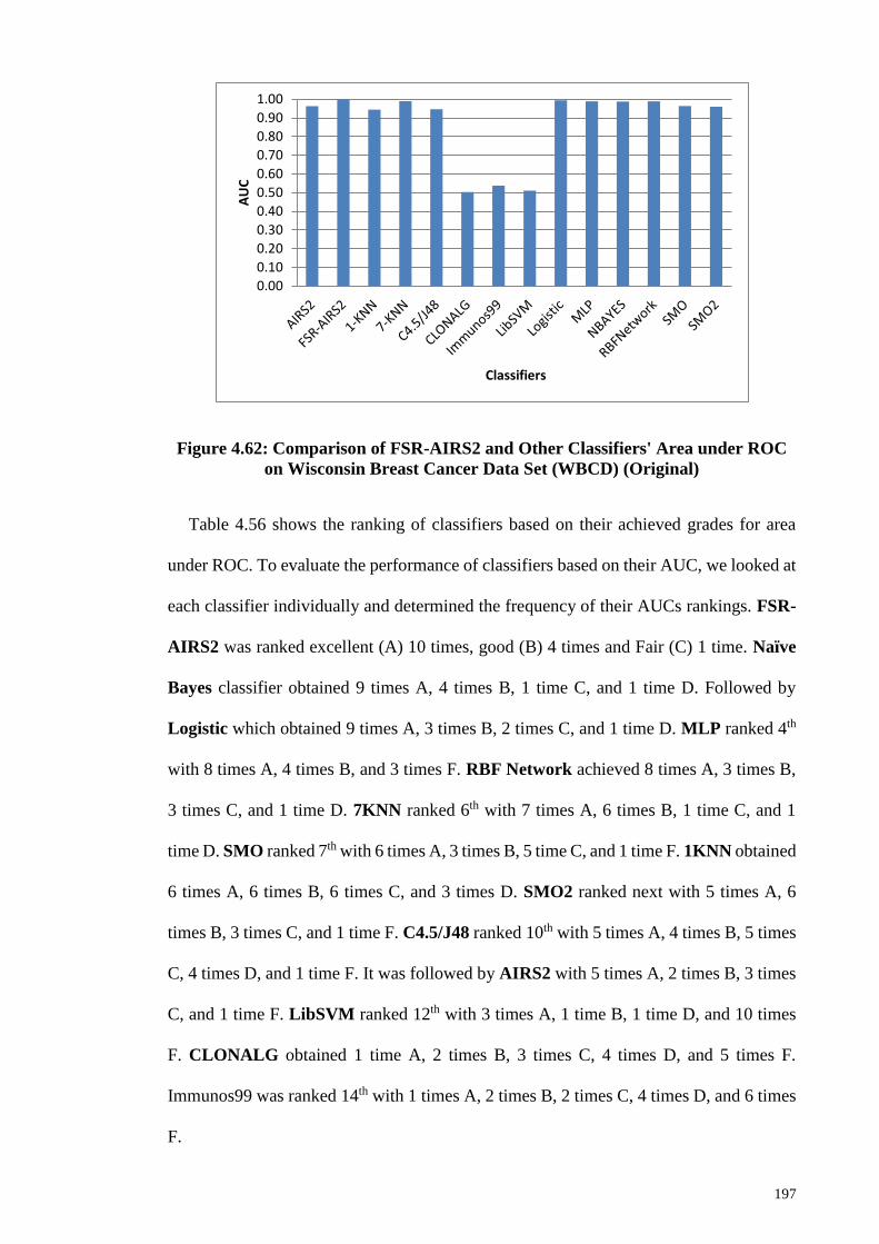
197
Figure 4.62: Comparison of FSR-AIRS2 and Other Classifiers' Area under ROC
on Wisconsin Breast Cancer Data Set (WBCD) (Original)
Table 4.56 shows the ranking of classifiers based on their achieved grades for area
under ROC. To evaluate the performance of classifiers based on their AUC, we looked at
each classifier individually and determined the frequency of their AUCs rankings. FSR-
AIRS2 was ranked excellent (A) 10 times, good (B) 4 times and Fair (C) 1 time. Naïve
Bayes classifier obtained 9 times A, 4 times B, 1 time C, and 1 time D. Followed by
Logistic which obtained 9 times A, 3 times B, 2 times C, and 1 time D. MLP ranked 4th
with 8 times A, 4 times B, and 3 times F. RBF Network achieved 8 times A, 3 times B,
3 times C, and 1 time D. 7KNN ranked 6th with 7 times A, 6 times B, 1 time C, and 1
time D. SMO ranked 7th with 6 times A, 3 times B, 5 time C, and 1 time F. 1KNN obtained
6 times A, 6 times B, 6 times C, and 3 times D. SMO2 ranked next with 5 times A, 6
times B, 3 times C, and 1 time F. C4.5/J48 ranked 10th with 5 times A, 4 times B, 5 times
C, 4 times D, and 1 time F. It was followed by AIRS2 with 5 times A, 2 times B, 3 times
C, and 1 time F. LibSVM ranked 12th with 3 times A, 1 time B, 1 time D, and 10 times
F. CLONALG obtained 1 time A, 2 times B, 3 times C, 4 times D, and 5 times F.
Immunos99 was ranked 14th with 1 times A, 2 times B, 2 times C, 4 times D, and 6 times
F.
0.00
0.10
0.20
0.30
0.40
0.50
0.60
0.70
0.80
0.90
1.00
AU
C
Classifiers
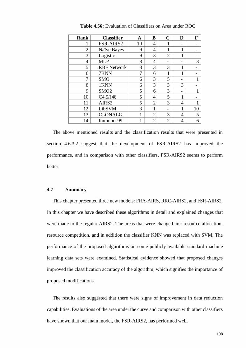
198
Table 4.56: Evaluation of Classifiers on Area under ROC
Rank Classifier A B C D F
1 FSR-AIRS2 10 4 1 - -
2 Naïve Bayes 9 4 1 1 -
3 Logistic 9 3 2 1 -
4 MLP 8 4 - - 3
5 RBF Network 8 3 3 1 -
6 7KNN 7 6 1 1 -
7 SMO 6 3 5 - 1
8 1KNN 6 3 3 3 -
9 SMO2 5 6 3 - 1
10 C4.5/J48 5 4 5 1 -
11 AIRS2 5 2 3 4 1
12 LibSVM 3 1 - 1 10
13 CLONALG 1 2 3 4 5
14 Immunos99 1 2 2 4 6
The above mentioned results and the classification results that were presented in
section 4.6.3.2 suggest that the development of FSR-AIRS2 has improved the
performance, and in comparison with other classifiers, FSR-AIRS2 seems to perform
better.
4.7 Summary
This chapter presented three new models: FRA-AIRS, RRC-AIRS2, and FSR-AIRS2.
In this chapter we have described these algorithms in detail and explained changes that
were made to the regular AIRS2. The areas that were changed are: resource allocation,
resource competition, and in addition the classifier KNN was replaced with SVM. The
performance of the proposed algorithms on some publicly available standard machine
learning data sets were examined. Statistical evidence showed that proposed changes
improved the classification accuracy of the algorithm, which signifies the importance of
proposed modifications.
The results also suggested that there were signs of improvement in data reduction
capabilities. Evaluations of the area under the curve and comparison with other classifiers
have shown that our main model, the FSR-AIRS2, has performed well.

199
As mentioned earlier, some classifiers were faster than FSR-AIRS2 and some slower
in running time. The running times of the FSR-AIRS2 algorithm on benchmark data sets
ranked somewhere among well-known classifiers.
This chapter presented details of FRA-AIRS2 and RRC-AIRS2 algorithms and
compared their results with that of the AIRS2. Results showed that both algorithms
performed well in comparison with the AIRS2.
The "no free lunch theorem" introduced by (Wolpert & Macready, 1997) is still valid,
according to this theorem no classifier can significantly outperform all other classifiers
across all problem domains. It is simply impossible to have a general purpose classifier
that can work on all datasets with highest accuracy, and in least amount of time.

200
CHAPTER 5: CONCLUSIONS AND FUTURE WORK
5.1 Conclusion
There is a huge request for new generations of tools to extract significant and useful
information from rapidly growing data. One of major tasks of data mining is classification
and results of Artificial Immune Recognition System (AIRS2) an immune inspired
algorithm has shown its potential for classification purposes. AIRS2 is a classifier
offering robust and powerful information processing capabilities. It has been shown that
AIRS2 has the potentials to perform better and therefore deserves to be investigated.
Performance of each classifier is measured with its classification accuracy and
efficiency and improving them was the goal of this thesis, therefore this research studied
and analyzed the algorithm of AIRS2. This study has pointed out to some issues that
needed to be addressed.
One of the problems occurred in the resource allocation method of AIRS, where a
linear function was used to determine the amount of resources that needed to be allocated,
and this linearity has increased the running time of AIRS2 and therefore reduced its
efficiency. In order to solve this linearity issue, this thesis replaced the linear function
with a fuzzy function.
Resource competition part of AIRS posed another problem, here, premature memory
cells were generated which were responsible for reduced accuracy. In order to solve this
problem, a new competition mechanism using real world tournament selection strategy
was utilized.
Further AIRS2 uses KNN as a classifier and that makes it severely vulnerable to the
presence of noise, irrelevant features, and the number of attributes. KNN also uses
majority voting and a drawback of this is that the classes with the more frequent instances

201
tend to dominate the prediction of the new instance. The consequence of using KNN was
ultimately reduction of classification accuracy. This thesis solved this problem with
replacing KNN with SVM, which is known as a robust and more accurate classifier.
The new algorithm was dubbed as FSR-AIRS2, its performance was evaluated and
compared with the results obtained with AIRS2 on 15 benchmark data sets obtained from
UCI machine learning repository. The comparison with AIRS2 showed that FSR-AIRS2
has statistically significantly increased the classification accuracy on almost all (14 out
of 15) benchmark data sets.
Comparing the results of FSR-AIRS2 with other classifiers showed that FSR-AIRS2
has achieved higher classification accuracy on majority of data sets. These results
indicated that the FSR-AIRS2 algorithm performs comparatively well in relation to other
classifiers.
Comparing the data reduction capability of FSR-AIRS2 with that of AIRS2 has shown
that FSR-AIRS2 achieved greater efficiency than AIRS2 without sacrificing accuracy.
Data reduction causes less runtime and this way increases the efficiency of the algorithm.
Of course data reduction depends on the domain, and there can be no assurance that FSR-
AIRS2 would keep the trend for all data sets.
While 3 classifiers performed faster in running time, FSR-AIRS2 was able to be faster
in most cases on the same benchmark data sets. This is of course encouraging, because it
shows that FSR-AIRS2 did not negatively affect the running time of the classifier so
much. The results suggest that FSR-AIRS2 is comparable to other classifiers based on the
running time. It is not surprising that when FSRARIRS2 has reduced the data set that we
see an increase in running time.

202
Comparing the AUCs obtained with FSR-AIRS2 to other classifiers showed that that
the FSR-AIRS2 has improved the performance, and in comparison with other classifiers,
FSR-AIRS2 seems to perform better.
5.2 Future Works
This thesis has introduced an improved version of artificial immune recognition
system dubbed as FSRARIS2. The focus of this study was to improve the performance of
AIRS2. As such, there is inevitably more to be done. This section discusses some of these
thoughts here.
5.2.1 Utilizing other Classifiers Instead of SVM
In order to improve the performance of the classifier, this study has utilized Support
Vector Machine instead of KNN, which has been used by the AIRS1 and AIRS2. The
obtained results were encouraging and promising as it has been shown in
chapter CHAPTER 4:. However, the search for a better classifier must continue because
it is highly demanded. Utilizing other well-known classifiers such as, but not limited to:
C4.5, Naïve Bayes, k-Means, and CART may improve the classification performance.
5.2.2 Fuzzy Control of Resources
This study used fuzzy logic to control resource allocation mechanism of the algorithm.
This concept could be extended to the resource competition mechanism as well which
may improve the quality of evolved memory cells and thus improve the performance of
the classifier. This study also recommends exploring other fuzzy methods for controlling
resources.

203
REFERENCES
Adya, M., & Collopy, F. (1998). How effective are neural networks at forecasting and
prediction? A review and evaluation. J. Forecasting, 17, 481-495.
Aggarwal, C. C. (2014a). Data classification: algorithms and applications: CRC Press.
Aggarwal, C. C. (2014b). Instance-Based Learning: A Survey. Data Classification:
Algorithms and Applications, 157.
Ahn, C. W. (2006). Advances in Evolutionary Algorithms: Theory, Design and
Practice: Springer.
Alpaydin, E. (2014). Introduction to machine learning: MIT press.
Antunes, M., Silva, C., Ribeiro, B., & Correia, M. (2011a). A hybrid AIS-SVM ensemble
approach for text classification. Paper presented at the International Conference
on Adaptive and Natural Computing Algorithms.
Antunes, M., Silva, C., Ribeiro, B., & Correia, M. (2011b). A hybrid AIS-SVM
ensemble approach for text classification Adaptive and Natural Computing
Algorithms (Vol. 6594, pp. 342-352). Berlin Heidelberg: Springer.
Aydin, I., Karakose, M., & Akin, E. (2011). A multi-objective artificial immune
algorithm for parameter optimization in support vector machine. Applied Soft
Computing, 11(1), 120-129.
Bach, F. R., Lanckriet, G. R., & Jordan, M. I. (2004). Multiple kernel learning, conic
duality, and the SMO algorithm. Paper presented at the Proceedings of the
twenty-first international conference on Machine learning.
Bache, K., & Moshe, L. (2013, June 2012). UCI Machine Learning Repository
Retrieved from http://archive.ics.uci.edu/ml
Bäck, T. (1995). Evolutionary Algorithms in Theory and Practice : Evolution
Strategies, Evolutionary Programming, Genetic Algorithms: Evolution
Strategies, Evolutionary Programming, Genetic Algorithms. New York: Oxford
University Press, USA.

204
Bäck, T., & Schwefel, H.-P. (1993). An overview of evolutionary algorithms for
parameter optimization. Evolutionary Computation, 1(1), 1-23.
Bandyopadhyay, S., & Pal, S. K. (2007). Classification and Learning Using Genetic
Algorithms: Applications in Bioinformatics and Web Intelligence: Springer
Berlin Heidelberg.
Bethlehem, J. G., & Van Der Heijden, P. G. M. (2000). COMPSTAT: Proceedings in
Computational Statistics ; 14th Symposium Held in Utrecht, The Netherlands,
2000 ; with 96 Tables. Heidelberg: Physica-Verlag.
Boggess, L., & Hamaker, J. S. (2003). The effect of irrelevant features on airs, an
artificial immune-based classifier. Intelligent Engineering Systems through
Artificial Neural Networks (ANNIE), 219-224.
Bongard, J. (2009). Biologically inspired computing. Computer(4), 95-98.
Bouckaert, R. R., Frank, E., Hall, M. A., Holmes, G., Pfahringer, B., Reutemann, P., &
Witten, I. H. (2010). WEKA---Experiences with a Java Open-Source Project.
The Journal of Machine Learning Research, 9999, 2533-2541.
Bradley, A. P. (1997). The use of the area under the ROC curve in the evaluation of
machine learning algorithms. Pattern Recognition, 30(7), 1145-1159.
Brownlee, J. (2005). Artificial immune recognition system (airs)-a review and analysis.
Center for Intelligent Systems and Complex Processes (CISCP), Faculty of
Information and Communication Technologies (ICT), Swinburne University of
Technology, Victoria, Australia.
Brownlee, J. (2011). Clever algorithms : nature-inspired programming recipes (1st ed.).
Raleigh, NC 27607, United States: Lulu Enterprises.
Burnet, S. F. M. (1959). The clonal selection theory of acquired immunity. Nashville,
Tennessee, USA: Cambridge University Press; Vanderbilt University Press
Nashville.
Cadenas, J. M., Garrido, M. C., Martínez, R., & Bonissone, P. P. (2012). OFP_CLASS:
a hybrid method to generate optimized fuzzy partitions for classification. Soft
Computing, 16(4), 667-682.

205
Cantú-Paz, E. (2000). Efficient and accurate parallel genetic algorithms (Vol. 1):
Springer.
Carter, J. H. (2000). The immune system as a model for pattern recognition and
classification. Journal of the American Medical Informatics Association, 7(1),
28-41.
Cendrowska, J. (1987). PRISM: An algorithm for inducing modular rules. International
Journal of Man-Machine Studies, 27(4), 349-370.
Chang, C.-C., & Lin, C.-J. (2011). (LIBSVM): A library for support vector machines.
ACM Transactions on Intelligent Systems and Technology, 2(3), 27:21--27:27.
Chauhan, S., Goel, V., & Dhingra, S. (2012). Pattern recognition system using MLP
neural networks. Pattern Recognition, 4(9), 43-46.
Chen, C. H., Xu, C., Bie, R. F., & Gao, X. Z. (2008). Artificial Immune Recognition
System for DNA Microarray Data Analysis. Paper presented at the Fourth
International Conference on Natural Computation: Icnc
Cheng, H.-P., Lin, Z.-S., Hsiao, H.-F., & Tseng, M.-L. (2010). Designing an Artificial
Immune System-Based Machine Learning Classifier for Medical Diagnosis. In
R. B. Z. Y. C. L. B. X. L. C. F. Zhu (Ed.), Information Computing and
Applications (Vol. 6377, pp. 333-341).
Chien, B.-C., Lin, J.-y., & Yang, W.-P. (2006). A classification tree based on
discriminant functions. Journal of Information Science and Engineering, 22(3),
573.
Chikh, M. A., Saidi, M., & Settouti, N. (2012). Diagnosis of Diabetes Diseases Using
an Artificial Immune Recognition System2 (AIRS2) with Fuzzy K-nearest
Neighbor. Journal of Medical Systems, 36(5), 2721-2729. doi:10.1007/s10916-
011-9748-4
Chou, J.-S., Cheng, M.-Y., & Wu, Y.-W. (2013). Improving classification accuracy of
project dispute resolution using hybrid artificial intelligence and support vector
machine models. Expert Systems with Applications, 40(6), 2263-2274.
doi:http://dx.doi.org/10.1016/j.eswa.2012.10.036
Cintra, M. E., Monard, M. C., & Camargo, H. A. (2013). On Rule Learning Methods: A
Comparative Analysis of Classic and Fuzzy Approaches Soft Computing: State
of the Art Theory and Novel Applications (pp. 89-104): Springer.

206
Cooke, D. E., & Hunt, J. E. (1995). Recognising promoter sequences using an artificial
immune system. Paper presented at the Proceedings of the Third International
Conference on Intelligent Systems for Molecular Biology (ISMB-95).
Cortes, C., & Vapnik, V. (1995). Support-vector networks. Machine Learning, 20(3),
273-297.
Cox, D. R. (1958). The regression analysis of binary sequences. Journal of the Royal
Statistical Society. Series B (Methodological), 215-242.
Das, R., & Sengur, A. (2010). Evaluation of ensemble methods for diagnosing of
valvular heart disease. Expert Systems with Applications, 37(7), 5110-5115.
doi:10.1016/j.eswa.2009.12.085
Dasgupta, D. (1998). An overview of artificial immune systems and their applications
from the book Artificial Immune System and Their Applications: Springer-
Verlag.
Dasgupta, D. (1999). Artificial Immune Systems and Their Applications (1st ed.).
Berlin: Springer-Verlag.
Dasgupta, D. (2006). Advances in artificial immune systems. Computational
Intelligence Magazine, IEEE, 1(4), 40-49.
Dasgupta, D., & Forrest, S. (1998). An anomaly detection algorithm inspired by the
immune system. from the book "Artificial Immune Systems and their
Applications", 262-277.
Dasgupta, D., Ji, Z., & Gonzalez, F. (2003, December 8-12, 2003). Artificial immune
system (AIS) research in the last five years. Paper presented at the Congress on
Evolutionary Computation Conference (CEC), Canberra, Australia.
Dasgupta, D., Yu, S., & Majumdar, N. (2003, July 12-16, 2003). MILA—multilevel
immune learning algorithm. Paper presented at the Genetic and Evolutionary
Computation Conference (GECCO), Chicago, Illinois.
Dasgupta, D., Yu, S., & Nino, F. (2011). Recent Advances in Artificial Immune
Systems: Models and Applications. Applied Soft Computing, 11(2), 1574-1587.
doi:10.1016/j.asoc.2010.08.024
207
De Castro, L. N., & Timmis, J. (2002a, May 2002). An artificial immune network for
multimodal function optimization. Paper presented at the Proceedings of the
Congress on Evolutionary Computation, Honolulu, HI, USA.
De Castro, L. N., & Timmis, J. (2002b). Artificial immune systems: a new
computational intelligence approach: Springer Verlag.
De Castro, L. N., & Timmis, J. (2003). Artificial immune systems as a novel soft
computing paradigm. Soft Computing, 7(8), 526-544.
De Castro, L. N., & Von Zuben, F. J. (2000a). The clonal selection algorithm with
engineering applications. Paper presented at the Proceedings of GECCO, Las
Vegas, USA.
De Castro, L. N., & Von Zuben, F. J. (2000b). An evolutionary immune network for
data clustering. Paper presented at the Neural Networks, 2000. Proceedings.
Sixth Brazilian Symposium on.
De Castro, L. N., & Von Zuben, F. J. (2001). Immune and neural network models:
theoretical and empirical comparisons. International Journal of Computational
Intelligence and Applications, 1(03), 239-257.
De Castro, L. N., & Von Zuben, F. J. (2002). Learning and optimization using the
clonal selection principle. IEEE Transactions on Evolutionary Computation,
6(3), 239-251.
De Jong, K. A. (2006). Evolutionary computation: a unified approach (Vol.
262041944): MIT press Cambridge.
Deng, Z.-l., Tan, G.-z., He, P., & Ye, J.-x. (2014). A fuzzy logic resource allocation and
memory cell pruning based artificial immune recognition system. Journal of
Central South University, 21, 610-617.
Dervilis, N., Choi, M., Taylor, S., Barthorpe, R., Park, G., Farrar, C., & Worden, K.
(2014). On damage diagnosis for a wind turbine blade using pattern recognition.
Journal of sound and vibration, 333(6), 1833-1850.
Dorff, K. C., Chambwe, N., Srdanovic, M., & Campagne, F. (2010). BDVal:
reproducible large-scale predictive model development and validation in high-
throughput datasets. Bioinformatics, 26(19), 2472-2473.
208
Drozda, M., Schaust, S., Schildt, S., & Szczerbicka, H. (2011). Priming: making the
reaction to intrusion or fault predictable. Natural computing, 10(1), 243-274.
doi:10.1007/s11047-010-9219-8
Dua, S., & Du, X. (2011). Data Mining and Machine Learning in Cybersecurity. Boca
Raton, FL, USA: Auerbach Publishers, Incorporated.
Duch, W. (2000). Datasets used for classification: comparison of results. Online:
http://www.phys.uni.torun.pl/kmk/projects/datasets.html.
Duda, R. O., & Hart, P. E. (1973). Pattern classification and scene analysis (Vol. 3):
Wiley New York.
Džeroski, S. (2010). Relational Data Mining. In O. Maimon & L. Rokach (Eds.), Data
Mining and Knowledge Discovery Handbook (pp. 887-911): Springer US.
Eiben, A. E., & Smith, J. E. (2008). Introduction to evolutionary computing (natural
computing series). Berlin: Srpinger-Verlag Berlin, Heidelberg.
EL-Manzalawy, Y., & Honavar, V. (2005). WLSW: Integrating LibSVM into WEKA
Environment. Retrieved from http://www.cs.iastate.edu/~yasser/wlsvm
Elsayed, S. A. M., Rajasekaran, S., & Ammar, R. A. (2012). An artificial immune
system approach to associative classification Computational Science and Its
Applications–ICCSA 2012 (pp. 161-171): Springer.
Farmer, J. D., Packard, N. H., & Perelson, A. S. (1986). The immune system,
adaptation, and machine learning. Physica D: Nonlinear Phenomena, 22(1),
187-204.
Fawcett, T. (2006). An introduction to ROC analysis. Pattern Recognition Letters,
27(8), 861-874.
Felicísimo, Á. M., Cuartero, A., Remondo, J., & Quirós, E. (2013). Mapping landslide
susceptibility with logistic regression, multiple adaptive regression splines,
classification and regression trees, and maximum entropy methods: a
comparative study. Landslides, 10(2), 175-189.
Feyyad, U. M. (1996). Data mining and knowledge discovery: making sense out of data.
IEEE Expert, 11(5), 20-25.

209
Fisher, R. A. (1936). The use of multiple measurements in taxonomic problems. Annals
of eugenics, 7(2), 179-188.
Fogel, L. J., Owens, A. J., & Walsh, M. J. (1966). Artificial intelligence through
simulated evolution. New York: Wiley & Sons.
Forouzideh, N., Mahmoudi, M. T., & Badie, K. (2011). Organizational texts
classification using artificial immune recognition systems. Paper presented at the
IEEE Symposium on Computational Intelligence in Bioinformatics and
Computational Biology (CIBCB).
Forsyth, R. (1990). PC/Beagle User's Guide. BUPA Medical Research Ltd.
Frank, A., & Asuncion, A. (2010, 2010). UCI Machine Learning Repository Retrieved
from http://archive.ics.uci.edu/ml
Freitas, A. A., & Timmis, J. (2007). Revisiting the foundations of artificial immune
systems for data mining. Evolutionary Computation, IEEE Transactions on,
11(4), 521-540.
Garrett, S. M. (2005). How do we evaluate artificial immune systems? Evolutionary
Computation, 13(2), 145-177.
Gelgi, F., Vadrevu, S., & Davulcu, H. (2007). Fixing weakly annotated web data using
relational models. Lecture Notes in Computer Science, 4607, 385.
Ghosh, A., & Jain, L. C. (2005). Evolutionary Computation in Data Mining. Berlin,
Heidelberg: Springer.
Giles, J. (2005). Internet encyclopaedias go head to head. Nature, 438(7070), 900-901.
Glickman, M., Balthrop, J., & Forrest, S. (2005). A machine learning evaluation of an
artificial immune system. Evolutionary Computation, 13(2), 179-212.
Goebel, M., & Gruenwald, L. (1999). A survey of data mining and knowledge
discovery software tools. ACM SIGKDD Explorations Newsletter, 1(1), 20-33.
Gokgoz, E., & Subasi, A. (2015). Comparison of decision tree algorithms for EMG
signal classification using DWT. Biomedical Signal Processing and Control, 18,
138-144. doi:http://dx.doi.org/10.1016/j.bspc.2014.12.005

210
Golzari, S. (2011). Utilisation of Exponential-based Resource Allocation and
Competition in Artificial Immune Recognition System. (PhD), Universiti Putra
Malaysia, Serdang.
Golzari, S., Doraisamy, S., Sulaiman, M. N., & Udzir, N. I. (2008). Effect of Nonlinear
Resource Allocation on AIRS Classifier Accuracy. Paper presented at the
Knowledge Management International Conference, Langkawi, Malaysia. <Go to
ISI>://WOS:000277018100104
Golzari, S., Doraisamy, S., Sulaiman, M. N., & Udzir, N. I. (2009a). Improving the
Accuracy of AIRS by Incorporating Real World Tournament Selection in
Resource Competition Phase. Trondheim, Norway IEEE
Golzari, S., Doraisamy, S., Sulaiman, M. N., & Udzir, N. I. (2009b). Incorporation of
Adapted Real World Tournament Selection into Artificial Immune Recognition
System Studies in Computational Intelligence (Vol. 214, pp. 329-334). Berlin,
Heidelberg: Springer
Golzari, S., Doraisamy, S., Sulaiman, M. N., & Udzir, N. I. (2011). An efficient and
effective immune based classifier. Journal of Computer Science, 7(2), 148-153.
Golzari, S., Doraisamy, S., Sulaiman, M. N., Udzir, N. I., & Norowi, N. M. (2008).
Artificial Immune Recognition System with Nonlinear Resource Allocation
Method and Application to Traditional Malay Music Genre Classification. In P.
J. Bentley, D. Lee, & S. Jung (Eds.), Artificial Immune Systems (Vol. 5132, pp.
132-141). Berlin Heidelberg: Springer.
Goodman, D. E., Boggess, L., & Watkins, A. (2002). Artificial immune system
classification of multiple-class problems. Proceedings of the Artificial Neural
Networks in Engineering ANNIE, 2, 179-183.
Goodman, D. E., Boggess, L., & Watkins, A. (2003, July 20-24, 2003). An investigation
into the source of power for AIRS, an artificial immune classification system.
Paper presented at the International Joing Conference on Neural Networks,
Portland, Oregon.
Gorman, R. P., & Sejnowski, T. J. (1988). Analysis of hidden units in a layered network
trained to classify sonar targets. Neural Networks, 1(1), 75-89.
Graaff, A. J., & Engelbrecht, A. P. (2011). Using sequential deviation to dynamically
determine the number of clusters found by a local network neighbourhood

211
artificial immune system. Applied Soft Computing, 11(2), 2698-2713.
doi:10.1016/j.asoc.2010.10.017
Grauman, K., & Darrell, T. (2005). The pyramid match kernel: Discriminative
classification with sets of image features. Paper presented at the Computer
Vision, 2005. ICCV 2005. Tenth IEEE International Conference on.
Greensmith, J., Aickelin, U., & Tedesco, G. (2010). Information fusion for anomaly
detection with the dendritic cell algorithm. Information Fusion, 11(1), 21-34.
doi:10.1016/j.inffus.2009.04.006
Hadarean, L., Bansal, K., Jovanović, D., Barrett, C., & Tinelli, C. (2014). A Tale of
Two Solvers: Eager and Lazy Approaches to Bit-Vectors. In A. Biere & R.
Bloem (Eds.), Computer Aided Verification (Vol. 8559, pp. 680-695): Springer
International Publishing.
Hamaker, J. S., & Boggess, L. (2004). Non-euclidean distance measures in AIRS, an
artificial immune classification system.
Han, J., & Kamber, M. (2006). Data Mining Concepts and Techniques (2nd ed.):
Morgan Kaufman - Diane Cerra.
Han, J., Kamber, M., & Pei, J. (2012). Data Mining Concepts and Techniques (3rd ed.).
Waltham, MA, USA: Morgan Kaufman.
Hanke, M., Halchenko, Y. O., Sederberg, P. B., Hanson, S. J., Haxby, J. V., &
Pollmann, S. (2009). PyMVPA: A python toolbox for multivariate pattern
analysis of fMRI data. Neuroinformatics, 7(1), 37-53.
Harmer, P. K., Williams, P. D., Gunsch, G. H., & Lamont, G. B. (2002). An artificial
immune system architecture for computer security applications. Evolutionary
Computation, IEEE Transactions on, 6(3), 252-280.
Harrell, F. E. (2013). Regression modeling strategies: with applications to linear
models, logistic regression, and survival analysis: Springer Science & Business
Media.
Hart, E., & Ross, P. (2004). Studies on the implications of shape-space models for
idiotypic networks Artificial Immune Systems (Lecture Notes in Computer
Science ed., Vol. 3239, pp. 413-426): Springer.

212
Hart, E., & Timmis, J. (2008). Application areas of AIS: The past, the present and the
future. Applied Soft Computing, 8(1), 191-201.
Hendrickx, I., & Van den Bosch, A. (2005, October 3-7). Hybrid algorithms with
instance-based classification Paper presented at the Machine Learning: ECML
2005: 16th European Conference on Machine Learning, Porto, Portugal.
Hmeidi, I., Hawashin, B., & El-Qawasmeh, E. (2008). Performance of KNN and SVM
classifiers on full word Arabic articles. Advanced Engineering Informatics,
22(1), 106-111. doi:http://dx.doi.org/10.1016/j.aei.2007.12.001
Hofmeyr, S. A., & Forrest, S. (2000). Architecture for an artificial immune system.
Evolutionary Computation, 8(4), 443-473.
Holland, J. (1975). Adaptation in Natural and Artificial systems. Ann Arbor: The
University of Michigan Press.
Hong, Z.-Q., & Yang, J.-Y. (1991). Optimal discriminant plane for a small number of
samples and design method of classifier on the plane. Pattern Recognition,
24(4), 317-324.
Hsu, C.-W., Chang, C.-C., & Lin, C.-J. (2003). A practical guide to support vector
classification.
Hu, J., Li, D., Duan, Q., Han, Y., Chen, G., & Si, X. (2012). Fish species classification
by color, texture and multi-class support vector machine using computer vision.
Computers and Electronics in Agriculture, 88, 133-140.
Huang, D. S., Gan, Y., Bevilacqua, V., & Figueroa, J. C. (2011). Advanced Intelligent
Computing: 7th International Conference, ICIC 2011, Zhengzhou, China,
August 11-14, 2011. Revised Selected Papers: Springer.
Huang, M.-L., Hung, Y.-H., Lee, W.-M., Li, R., & Wang, T.-H. (2012). Usage of case-
based reasoning, neural network and adaptive neuro-fuzzy inference system
classification techniques in breast cancer dataset classification diagnosis.
Journal of Medical Systems, 36(2), 407-414.
Igawa, K., & Ohashi, H. (2009). A negative selection algorithm for classification and
reduction of the noise effect. Applied Soft Computing, 9(1), 431-438.
doi:10.1016/j.asoc.2008.05.003

213
International-Electrothechnical-Commission. (1997). Industrial Porcess Measurement
and Control: Fuzzy Control Programming IEC, IEC
1131(http://www.fuzzytech.com/binaries/ieccd1.pdf), 53.
Jackson, S. L. (2012). Statistics Plain and Simple, 3rd ed: WADSWORTH Incorporated
FULFILLMENT.
Jenhani, I., & Elouedi, Z. (2012). Re-visiting the artificial immune recognition system: a
survey and an improved version. Artificial Intelligence Review, 1-13.
doi:10.1007/s10462-012-9360-0
Jerne, N. K. (1974). Towards a network theory of the immune system. Annales d'
Immunologie (Inst. Past.), 125C (1-2), 373-389.
Kalita, M., & Sarma, K. K. (2015). Wavelet and Learning Based Image Compression
Systems Advances in Communication and Computing (pp. 61-72): Springer.
Kantardzic, M. (2011). Data mining : concepts, models, methods and algorithms.
Oxford: John Wiley & Sons.
Kara, S., Aksebzeci, B. H., Kodaz, H., Güneş, S., Kaya, E., & Ozbilge, H. (2009).
Medical application of information gain-based artificial immune recognition
system (IG-AIRS): Classification of microorganism species. Expert Systems
with Applications, 36(3), 5168-5172. doi:10.1016/j.eswa.2008.06.029
Kecman, V. (2001). Learning and Soft Computing, Support Vector Machines, Neural
Networks, and Fuzzy Logic Models. Cambridge, Massachusetts, London,
England: The MIT Press.
Keller, J. M., Gray, M. R., & Givens, J. A. (1985). A fuzzy k-nearest neighbor
algorithm. IEEE Transactions on Systems, Man, and Cybernetics(4), 580-585.
Khashei, M., Zeinal Hamadani, A., & Bijari, M. (2012). A novel hybrid classification
model of artificial neural networks and multiple linear regression models. Expert
Systems with Applications, 39(3), 2606-2620.
doi:http://dx.doi.org/10.1016/j.eswa.2011.08.116
Kim, J. W., Bentley, P. J., Aickelin, U., Greensmith, J., Tedesco, G., & Twycross, J.
(2007). Immune system approaches to intrusion detection–a review. Natural
computing, 6(4), 413-466.
214
Kim, T.-h., Adeli, H., Cuzzocrea, A., Arslan, T., Zhang, Y., Ma, J., . . . Song, X. (2011).
Database Theory and Application, Bio-Science and Bio-Technology:
International Conferences, DTA and BSBT 2011, Held as Part of the Future
Generation Information Technology Conference, FGIT 2011, in Conjunction
with GDC 2011, Jeju Island, Korea, December 8-10, 2011. Proceedings (Vol.
258): Springer.
Kleinbaum, D. G., & Klein, M. (2010). Logistic Regression: A Self-Learning Text:
Springer New York.
Knight, T., & Timmis, J. (2001). AINE: An Immunological Approach to Data Mining.
Paper presented at the Proceedings of the 2001 IEEE International Conference
on Data Mining.
Knight, T., & Timmis, J. (2001). Assessing the performance of the resource limited
artificial immune system AINE. Retrieved from Canterburry, kent, UK
Knight, T., & Timmis, J. (2003). A Multi-layered immune inspired machine learning
algorithm. Applications and Science in Soft Computing, 195-202.
Kodaz, H., Babaoğlu, İ., & İşcan, H. (2009). Thyroid disease diagnosis using Artificial
Immune Recognition System (AIRS). Paper presented at the Proceedings of the
2nd International Conference on Interaction Sciences: Information Technology,
Culture and Human.
Kohonen, T. (1990). The self-organizing map. Proceedings of the IEEE, 78(9), 1464-
1480.
Kowalik, J., & Puźniakowski, T. (2012). Using OpenCL: Programming Massively
Parallel Computers. Amsterdam, Netherlands: IOS Press BV.
Kramer, O. (2008). Self-Adaptive Heuristics for Evolutionary Computation (J. Kacprzyk
Ed. Vol. 147). Berlin: Springer.
Kress, M. (2010). Intelligent Business Process Optimization for the Service Industry:
KIT Scientific Publishing.
Kuo, R., Chen, C., Liao, T. W., & Tien, F. (2013). Hybrid of artificial immune system
and particle swarm optimization-based support vector machine for Radio
Frequency Identification-based positioning system. Computers & Industrial
Engineering, 64(1), 333-341.
215
Latifoǧlu, F., Kodaz, H., Kara, S., & Güneş, S. (2007). Medical application of Artificial
Immune Recognition System (AIRS): Diagnosis of atherosclerosis from carotid
artery Doppler signals. Computers in Biology and Medicine, 37(8), 1092-1099.
doi:10.1016/j.compbiomed.2006.09.009
Laura Auria, R. A. M. (2008). Support Vector Machines (SVM) as a Technique for
Solvency Analysis. The Open Access Publication Server of the ZBW – Leibniz
Information Centre for Economics. Retrieved from
http://www.econstor.eu/bitstream/10419/27334/1/576821438.PDF
Le, X., & Mo-Yuen, C. (2008, 20-24 July 2008). Distribution Fault Diagnosis using a
Hybrid Algorithm of Fuzzy Classification and Artificial Immune Systems. Paper
presented at the Power and Energy Society General Meeting - Conversion and
Delivery of Electrical Energy in the 21st Century, 2008 IEEE, Pittsburgh, PA.
Lee, S., Soak, S., Kim, K., Park, H., & Jeon, M. (2008). Statistical properties analysis of
real world tournament selection in genetic algorithms. Applied Intelligence,
28(2), 195-205.
Leitão, P., Barbosa, J., & Trentesaux, D. (2012). Bio-inspired multi-agent systems for
reconfigurable manufacturing systems. Engineering Applications of Artificial
Intelligence, 25(5), 934-944.
Leung, K., Cheong, F., & Cheong, C. (2007a). Consumer credit scoring using an
artificial immune system algorithm. Paper presented at the Evolutionary
Computation, 2007. CEC 2007. IEEE Congress on.
Leung, K., Cheong, F., & Cheong, C. (2007b). Generating compact classifier systems
using a simple artificial immune system. Systems, Man, and Cybernetics, Part
B: Cybernetics, IEEE Transactions on, 37(5), 1344-1356.
Li, F., Xu, L. D., Jin, C., & Wang, H. (2011). Structure of Multi-Stage Composite
Genetic Algorithm (MSC-GA) and its performance. Expert Systems with
Applications, 38(7), 8929-8937.
doi:http://dx.doi.org/10.1016/j.eswa.2011.01.110
Li, Q., Salman, R., Test, E., Strack, R., & Kecman, V. (2013). Parallel multitask cross
validation for Support Vector Machine using GPU. Journal of Parallel and
Distributed Computing, 73(3), 293-302.
Lichman, M. (2013). UCI machine learning repository: University of California, Irvine,
School of Information and Computer Sciences.

216
Lin, H.-C., Su, C.-T., & Wang, P.-C. (2011). An Application of Artificial Immune
Recognition System for Prediction of Diabetes Following Gestational Diabetes.
Journal of Medical Systems, 35(3), 283-289.
Liu, D., Li, T., & Liang, D. (2014). Incorporating logistic regression to decision-
theoretic rough sets for classifications. International Journal of Approximate
Reasoning, 55(1), 197-210.
Liu, J. (2013). Radial Basis Function (RBF) Neural Network Control for Mechanical
Systems: Design, Analysis and Matlab Simulation: Springer Berlin Heidelberg.
Machaka, P., Mabande, T., & Bagula, A. (2012). Monitoring of a Large Wi-Fi Hotspots
Network: Performance Investigation of Soft Computing Techniques Bio-
Inspired Models of Networks, Information, and Computing Systems (pp. 155-
162): Springer.
Mantas, C. J., & Abellán, J. (2014). Credal-C4. 5: Decision tree based on imprecise
probabilities to classify noisy data. Expert Systems with Applications, 41(10),
4625-4637.
Mao, C.-H., Lee, H.-M., & Yeh, C.-F. (2011). Adaptive e-mails intention finding
system based on words social networks. Journal of Network and Computer
Applications, 34(5), 1615-1622. doi:10.1016/j.jnca.2011.03.030
Mark Hall, Eibe Frank, Geoffrey Holmes, Bernhard Pfahringer, Peter Reutemann, &
Witten, I. H. (2009). The WEKA Data Mining Software: An Update. SIGKDD
Explorations, 11(1).
Marwah, G., & Boggess, L. (2002). Artificial immune systems for classification: Some
issues, University of kent at Canterbury.
Mastrogiannis, N., Boutsinas, B., & Giannikos, I. (2009). A method for improving the
accuracy of data mining classification algorithms. Computers & Operations
Research, 36(10), 2829-2839. doi:http://dx.doi.org/10.1016/j.cor.2008.12.011
Meng, L., van der Putten, P., & Wang, H. (2005). A comprehensive benchmark of the
artificial immune recognition system (AIRS). Paper presented at the International
Conference on Advanced Data Mining and Applications.
Mera, N. S., Ingham, D. B., & Elliott, L. (2004). Genetic Algorithms and Their
Application To The Identification Of Hydraulic Properties Of Rocks: Springer.

217
Miller, B. L., & Goldberg, D. E. (1995). Genetic Algorithms, Tournament Selection,
and the Effects of Noise. Complex systems, 9(3), 193-212.
Mishra, V. N., Dwivedi, R., & Das, R. R. (2013). Gases/Odors Identification With
Artificial Immune Recognition System Using Thick Film Gas Sensor Array
Responses. Sensors Journal, IEEE, 13(8), 3039-3045.
doi:10.1109/JSEN.2013.2257741
Mitchell, M., & Taylor, C. E. (1999). Evolutionary computation: an overview. Annual
Review of Ecology and Systematics, 30, 593-616.
Nasaroui, O., Gonzalez, F., & Dasgupta, D. (2002). The fuzzy artificial immune system:
Motivations, basic concepts, and application to clustering and web profiling.
Paper presented at the International Conference on Fuzzy Systems FUZZ-IEEE,
Honolulu, Hawaii.
Nisbet, R., Elder, J., & Miner, G. (2009). Handbook of Statistical Analysis and Data
Mining Applications. Printed in Canada: Elsevier Science.
Nivre, J., Hall, J., Nilsson, J., Chanev, A., Eryigit, G., Kübler, S., . . . Marsi, E. (2007).
MaltParser: A language-independent system for data-driven dependency parsing.
Natural Language Engineering, 13(02), 95-135.
Osyk, B. A., Hung, M. S., & Madey, G. R. (1994). A neural network model for fault
detection in conjunction with a programmable logic controller. Journal of
Intelligent Manufacturing, 5(2), 67-78.
Pang-Ning Tan, M. S., Viping Kumar. (2006). Introduction To Data Mining: Pearson
Addison Wesley.
Pappa, G. L., & Freitas, A. A. (2010). Automating the Design of Data Mining
Algorithms. Retrieved from http://www.myilibrary.com?id=283570
Perelson, A. S. (1989). Immune network theory. Immunological Reviews, 110(1), 5-36.
Pham, H. N. A., & Triantaphyllou, E. (2011). A meta-heuristic approach for improving
the accuracy in some classification algorithms. Computers & Operations
Research, 38(1), 174-189. doi:http://dx.doi.org/10.1016/j.cor.2010.04.011

218
Phinyomark, A., Quaine, F., Charbonnier, S., Serviere, C., Tarpin-Bernard, F., &
Laurillau, Y. (2013). EMG feature evaluation for improving myoelectric pattern
recognition robustness. Expert Systems with Applications, 40(12), 4832-4840.
Platt, J. C. (1999). 12 Fast training of support vector machines using sequential
minimal optimization. Paper presented at the Advances in kernel methods.
Polat, K., & Güneş, S. (2007). An improved approach to medical data sets
classification: artificial immune recognition system with fuzzy resource
allocation mechanism. Expert Systems, 24(4), 252-270.
Polat, K., & Güneş, S. (2008). Artificial immune recognition system with fuzzy
resource allocation mechanism classifier, principal component analysis and FFT
method based new hybrid automated identification system for classification of
EEG signals. Expert Systems with Applications, 34(3), 2039-2048.
doi:10.1016/j.eswa.2007.02.009
Polat, K., Güneş, S., & Tosun, S. (2006). Diagnosis of heart disease using artificial
immune recognition system and fuzzy weighted pre-processing. Pattern
Recognition, 39(11), 2186-2193. doi:10.1016/j.patcog.2006.05.028
Polat, K., Şahan, S., & Güneş, S. (2006). A new method to medical diagnosis: Artificial
immune recognition system (AIRS) with fuzzy weighted pre-processing and
application to ECG arrhythmia. Expert Systems with Applications, 31(2), 264-
269. doi:10.1016/j.eswa.2005.09.019
Polat, K., Şahan, S., & Güneş, S. (2007). A novel hybrid method based on artificial
immune recognition system (AIRS) with fuzzy weighted pre-processing for
thyroid disease diagnosis. Expert Systems with Applications, 32(4), 1141-1147.
doi:10.1016/j.eswa.2006.02.007
Polat, K., Şahan, S., Kodaz, H., & Güneş, S. (2007). Breast cancer and liver disorders
classification using artificial immune recognition system (AIRS) with
performance evaluation by fuzzy resource allocation mechanism. Expert Systems
with Applications, 32(1), 172-183. doi:10.1016/j.eswa.2005.11.024
Prasad, K. N. (2010). Micronutrients in Health and Disease: Taylor & Francis - CRC
Press.
Quinlan, J. R. (1986). Induction of decision trees. Machine Learning, 1(1), 81-106.

219
Quinlan, J. R. (1993). C4. 5: programs for machine learning (Vol. 1): Morgan
kaufmann.
Quinlan, J. R. (2014). C4. 5: programs for machine learning: Elsevier.
Rahmani, A., & Helmi, H. (2008). EIN-WUM an AIS-based Algorithm for Web Usage
Mining. Paper presented at the 10th annual conference on Genetic and
evolutionary computation, Atlanta, Georgia, USA.
Rechenberg, I. (1973). Evolutionsstrategie-Optimierung technischer Systeme nach
Prinzipien der biologischen Evolution. Stuttgart: Frommann-Holzboog.
Şahan, S., Polat, K., Kodaz, H., & Güneş, S. (2007). A new hybrid method based on
fuzzy-artificial immune system and k-nn algorithm for breast cancer diagnosis.
Computers in Biology and Medicine, 37(3), 415-423.
Saidi, M., Chikh, M. A., & Settouti, N. (2011). Automatic identification of Diabetes
Diseases using a Modified Artificial Immune Recognition System2 (MAIRS2).
Paper presented at the Conference internationale sur l ‘informatique et ses
applications, Saida, Algeria.
Seeker, A., & Freitas, A. A. (2007, 25-28 September). Wairs: Improving Classification
Accuracy by Weighting Attributes in the Airs classifier. Paper presented at the
Congress on Evolutionary Computation, Singapore.
Shafigh, P., Hadi, S. Y., & Sohrab, E. (2013). Gravitation based classification.
Information sciences, 220(0), 319-330.
doi:http://dx.doi.org/10.1016/j.ins.2012.07.033
Shahid, R., Bertazzon, S., Knudtson, M., & Ghali, W. (2009). Comparison of distance
measures in spatial analytical modeling for health service planning. BMC Health
Services Research, 9(1), 200.
Shamshirband, S., Hessam, S., Javidnia, H., Amiribesheli, M., Vahdat, S., Petković, D.,
. . . Kiah, M. L. M. (2014). Tuberculosis Disease Diagnosis Using Artificial
Immune Recognition System. International journal of medical sciences, 11(5),
508.
Shepherd, A. d. J. (2012). Second-Order Methods for Neural Networks: Fast and
Reliable Training Methods for Multi-Layer Perceptrons: Springer London.

220
Siebert, J. P. (1987). Vehicle recognition using rule based methods.
Siegler, R. S. (1976). Three aspects of cognitive development. Cognitive psychology,
8(4), 481-520.
Sigillito, V. G., Wing, S. P., Hutton, L. V., & Baker, K. B. (1989). Classification of
radar returns from the ionosphere using neural networks. Johns Hopkins APL
Technical Digest, 10(3), 262-266.
Siniscalchi, S. M., Yu, D., Deng, L., & Lee, C.-H. (2013). Exploiting deep neural
networks for detection-based speech recognition. Neurocomputing, 106, 148-
157.
Sivanandam, S. N., & Deepa, S. N. (2007). Introduction to Genetic Algorithms. Berlin,
Heidelberg: Springer Publishing Company, Incorporated.
Smith, J. W., Everhart, J., Dickson, W., Knowler, W., & Johannes, R. (1988). Using the
ADAP learning algorithm to forecast the onset of diabetes mellitus. Paper
presented at the Proceedings of the Annual Symposium on Computer
Application in Medical Care.
Soman, K., Diwakar, S., & Ajay, V. (2006). Insight into data mining theory and
practice: PHI Learning Pvt. Ltd.
Sompayrac, L. (2012). How the immune system works. Chichester, West Sussex;
Hoboken, NJ: Wiley-Blackwell.
Statsoft. (2013). Support Vector Machines. Retrieved from
http://www.statsoft.com/textbook/support-vector-machines/
Stepney, S., Smith, R. E., Timmis, J., & Tyrrell, A. M. (2004). Towards a conceptual
framework for artificial immune systems Artificial Immune Systems (pp. 53-64):
Springer.
Street, W. N., Wolberg, W. H., & Mangasarian, O. L. (1993). Nuclear feature
extraction for breast tumor diagnosis. Paper presented at the IS&T/SPIE's
Symposium on Electronic Imaging: Science and Technology.
Strzelecki, M., Szczypinski, P., Materka, A., & Klepaczko, A. (2013). A software tool
for automatic classification and segmentation of 2D/3D medical images. Nuclear

221
Instruments and Methods in Physics Research Section A: Accelerators,
Spectrometers, Detectors and Associated Equipment, 702, 137-140.
Sundararajan, N., Saratchandran, P., & Li, Y. (2013). Fully Tuned Radial Basis
Function Neural Networks for Flight Control (Vol. 12): Springer Science &
Business Media.
SVMS.org. (2010). Introduction to Support Vector Machines,
http://www.svms.org/introduction.html. 2011(January 1st), 1.
Swets, J. A., Dawes, R. M., & Monahan, J. (2000). Better decisions through science.
Scientific American, 283, 82-87.
Swiderski, B., Kurek, J., & Osowski, S. (2012). Multistage classification by using
logistic regression and neural networks for assessment of financial condition of
company. Decision Support Systems, 52(2), 539-547.
Tang, N., & Vemuri, V. R. (2005). An artificial immune system approach to document
clustering. Paper presented at the ACM symposium on Applied computing.
Tape, T. G. (2013). Interpreting Diagnosis Test. Retrieved from
http://gim.unmc.edu/dxtests/default.htm
Tarakanov, A. O., & Skormin, V. A. (2002, May). Pattern recognition by
immunocomputing. Paper presented at the Proc. of the 2002 Congress on
Evolutionary Computation, CEC, Honolulu, Hawaii.
Tay, D., Poh, C. L., & Kitney, R. (2013, July 6). An evolutionary data-conscious
artificial immune recognition system. Paper presented at the Proceeding of the
fifteenth annual conference on Genetic and evolutionary computation
conference, Amsterdam, Netherlands.
Timmis, J. (2000). Artificial immune systems: a novel data analysis technique inspired
by the immune network theory. (PhD), University of Kent, UK. Retrieved from
http://kar.kent.ac.uk/21989/
Timmis, J., Hone, A., Stibor, T., & Clark, E. (2008). Theoretical advances in artificial
immune systems. Theoretical Computer Science, 403(1), 11-32.
Timmis, J., & Knight, T. (2002). Artificial immune systems: Using the immune system
as inspiration for data mining. Data Mining: A Heuristic Approach, 209-230.

222
Timmis, J., Knight, T., De Castro, L. N., & Hart, E. (2004). "An overview of artificial
immune systems." Computation in Cells and Tissues. Springer Berlin
Heidelberg, 51-91.
Timmis, J., & Neal, M. (2001). A resource limited artificial immune system for data
analysis. Knowledge-Based Systems, 14(3), 121-130.
Timmis, J., Neal, M., & Hunt, J. E. (2000). An artificial immune system for data
analysis. Biosystems, 55(1-3), 143-150.
Travers, P., Walport, M. J., Janeway, C., & Murphy, K. P. (2008). Janeway's
immunobiology. New York: Garland Science.
Turing, A. M. (1950). Computing machinery and intelligence. Mind, 433-460.
Van der Putten, P. (2010). On data mining in context: Cases, fusion and evaluation.
Leiden: Leiden Institute of Advanced Computer Science (LIACS).
Villalobos-Arias, M., Coello, C. A. C., & Hernández-Lerma, O. (2004). Convergence
analysis of a multiobjective artificial immune system algorithm Artificial
Immune Systems (pp. 226-235): Springer.
Watkins, A. (2001). AIRS: A Resource Limited Artificial Immune Classifier. (Master),
Mississipi State University, Mississipi, USA. Retrieved from
http://www.cse.msstate.edu/~andrew/research/publications/watkins_thesis.pdf
Watkins, A. (2005). Exploiting immunological metaphors in the development of serial,
parallel and distributed learning algorithms. (PhD), University of Kent,
Canterbury, UK. Retrieved from
http://www.cse.msstate.edu/~andrew/research/publications/watkins_phd_dissert
ation.pdf
Watkins, A., & Boggess, L. (2002, May 12-17, 2002). A new classifier based on
resource limited artificial immune systems. Paper presented at the World
Congress on Computational Intelligence Honolulu, HI, USA.
Watkins, A., & Timmis, J. (2002). Artificial immune recognition system (AIRS):
Revisions and refinements. Paper presented at the 1st International Conference
on Artificial Immune Systems, University of Kent at Canterbury, UK.

223
Watkins, A., & Timmis, J. (2004). Exploiting parallelism inherent in AIRS, an artificial
immune classifier. Artificial Immune Systems, 3239(Lecture Notes in Computer
Science), 427-438.
Watkins, A., Timmis, J., & Boggess, L. (2004). Artificial immune recognition system
(AIRS): An immune-inspired supervised learning algorithm. Genetic
Programming and Evolvable Machines, 5(3), 291-317.
Wei, C.-C. (2015). Comparing lazy and eager learning models for water level
forecasting in river-reservoir basins of inundation regions. Environmental
Modelling & Software, 63, 137-155.
White, J. A., & Garrett, S. M. (2003). Improved pattern recognition with artificial clonal
selection? Artificial Immune Systems (pp. 181-193): Springer.
Wikipedia. (2012). Artificial immune system. Retrieved from
http://en.wikipedia.org/wiki/Artificial_immune_system
Wikipedia. (2013). Adaptive immune system. Retrieved from
http://en.wikipedia.org/wiki/Adaptive_immune_system#cite_note-NIAID-5
Witten, I. H., Frank, E., & Hall, M. A. (2011). Data Mining Practical Machine
Learning Tools and Techniques (3rd ed.). Burlington, MA 01803, USA: Morgan
Kaufmann Publishers.
Wolberg, W. H., & Mangasarian, O. L. (1990). Multisurface method of pattern
separation for medical diagnosis applied to breast cytology. Proceedings of the
national academy of sciences, 87(23), 9193-9196.
Wolpert, D. H., & Macready, W. G. (1997). No free lunch theorems for optimization.
Evolutionary Computation, IEEE Transactions on, 1(1), 67-82.
Woolley, N., & Milanović, J. (2009). Application of AIS Based Classification
Algorithms to Detect Overloaded Areas in Power System Networks Artificial
Immune Systems (Vol. 5666, pp. 165-177): Springer.
Wu, X., Kumar, V., Quinlan, J. R., Ghosh, J., Yang, Q., Motoda, H., . . . Steinberg, D.
(2008). Top 10 algorithms in data mining. Knowledge and Information Systems,
14(1), 1-37. doi:10.1007/s10115-007-0114-2
224
Yang, M., Kiang, M., Chen, H., & Li, Y. (2012). Artificial Immune System for Illicit
Content Identification in Social Media. Journal of the American Society for
Information Science and Technology, 63(2), 256-269. doi:10.1002/asi.21673
Yi, P., Wu, Y., & Chen, J. (2011). Towards an Artificial Immune System for Detecting
Anomalies in Wireless Mesh Networks. China Communications, 8(3), 107-117.
Zhang, C., & Yi, Z. (2010). A danger theory inspired artificial immune algorithm for
on-line supervised two-class classification problem. Neurocomputing, 73(7-9),
1244-1255. doi:10.1016/j.neucom.2010.01.005
Zhao, H., Chen, W., Zeng, J., Shi, Y., & Qin, J. (2011). WPMSD: A Malicious Script
Detection Method Inspired by the Process of Immunoglobulin Secretion.
International Journal of Computational Intelligence Systems, 4(5), 788-796.
Zhao, W., & Davis, C. E. (2011). A modified artificial immune system based pattern
recognition approach—An application to clinical diagnostics. Artificial
Intelligence in Medicine, 52(1), 1-9. doi:10.1016/j.artmed.2011.03.001
Zheng, J., Chen, Y., & Zhang, W. (2010). A Survey of artificial immune applications.
Artificial Intelligence Review, 34(1), 19-34.
Zhu, F., & Guan, S. (2004). Feature selection for modular GA-based classification.
Applied Soft Computing, 4(4), 381-393.
doi:http://dx.doi.org/10.1016/j.asoc.2004.02.001
Zięba, M., Tomczak, J. M., Lubicz, M., & Świątek, J. (2014). Boosted SVM for
extracting rules from imbalanced data in application to prediction of the post-
operative life expectancy in the lung cancer patients. Applied Soft Computing,
14, 99-108.

225
LIST OF PUBLICATIONS AND PAPERS PRESENTED
Journals
2015
SAYBANI, MAHMOUD REZA; WAH, TEH YING; AGHABOZORGI, SAEED
REZA; SHAMSHIRBAND, SHAHABODDIN; MAT KIAHF, MISS LAIHA;
BALAS, VALENTINA EMILIA, Diagnosing Breast Cancer with an Improved
Artificial Immune Recognition System. Soft Computing 2015
SAYBANI, M. R.; SHAMSHIRBAND, SHAHABODDIN; GOLZARI, SHAHRAM;
TEH YING; AGHABOZORGI, SAEED; MAT KIAHF, MISS LAIHA;
VALENTINA EMILIA, RAIRS2 a new expert system for diagnosing
tuberculosis with real-world tournament selection mechanism inside artificial
immune recognition system. Medical & biological engineering & computing
2015, 1-15
SAYBANI, M. R.; SHAMSHIRBAND, SHAHABODDIN.; GOLZARI, SHAHRAM;
WAH, TEH YING; AGHABOZORGI, SAEED; POURHOSEINGHOLI,
MOHAMMAD AMIN; OLARIU, TEODORA, Diagnosing Tuberculosis With
a Novel Support Vector Machine-Based Artificial Immune Recognition
System. Iran Red Crescent Med J 2015, 17 (4), e24557
MARANDI, FERYAL; HATAM, AHMAD; SAYBANI, MAHMOUD REZA,
Diagnosing the Location of Gastric Ulcer by Thresholding Method Using the
Image Processing Technique. Journal of Applied Environmental and Biological
Sciences 2015, 5 (4), 239-246

226
MARANDI, FERYAL; HATAM, AHMAD; SAYBANI, MAHMOUD REZA,
Diagnosing Gastric Cancer and Ulcer Using Color Domain and Their
Classifications. J. Appl. Environ. Biol. Sci 2015, 5 (4), 239-246
MARANDI, FERYAL; HATAM, AHMAD; SAYBANI, MAHMOUD REZA,
Diagnosing Gastric Diseases by means of Fuzzy Method and Questionnaire.
gmp review 2015, 16, 4
2014
SADEGHIPOUR, EHSAN; SAYBANI, MAHMOUD REZA; BAHMANZADEH,
ZEINAB, CGBDE-Presentation of a New Combined Method for Optimization.
International Journal of Sciences: Basic and Applied Research (IJSBAR) 2014,
(8), 1504-1509
SADEGHIPOUR, EHSAN; SAYBANI, MAHMOUD REZA; BAHMANZADEH,
ZEINAB, CGBDE - Presentation of a New Combined Method for
Optimization. International Research Journal of Applied and Basic Sciences
2014, 8 (10), 1504-1509
SADEGHIPOUR, EHSAN; SAYBANI, MAHMOUD REZA, CGBDE - Presentation
of a New Combined Method for Optimization. Advances in Environmental
Biology 2014, 8 (11 Special), 1289-1294
SADEGHIPOUR, EHSAN; SAYBANI, MAHMOUD REZA, CGBDE - Presentation
of a New Combined Method for Optimization. Advances in Environmental
Biology 2014, 8 (11), 6

227
SADEGHIPOUR, EHSAN; SAYBANI, MAHMOUD REZA, Firefly algorithm with
the adaptive moving radius. In First National Conference on Innovative
Algorithms and their Applications in Engineering and Basic Sciences, Pardisan
Institute of Higher Education: Feridoonkenar, Iran, 2014
2012
DANESH AMIR SEYED, RODINA AHMAD, SAYBANI MAHMOUD REZA &
TAHIR AMJED 2011. Companies Approaches in Software Release Planning –
Based on Multiple Case Studies. Journal of Software, Vol 7, No 2 (2012), 471-
478.(SCOPUS, ProQuest, EBSCO cited publication).
2011
SAYBANI MAHMOUD REZA, WAH TEH YING, AMINI AMINEH &
AGHABOZORGI SAEED 2011a. Anomaly Detection and Prediction of
Sensors Faults in a Refinery using Data Mining Techniques and Fuzzy Logic.
Journal of Scientific Research and Essays Vol. 6(27), pp. 5685-5695, 16
November, 2011 DOI: 10.5897/SRE11.33 . (ISI cited publication).
SAYBANI MAHMOUD REZA, WAH TEH YING, AMINI AMINEH ,
AGHABOZORGI SAEED & LAHSASNA ADEL 2011b. Applications of
Support Vector Machines in Oil Refineries: A Survey. International Journal of
the Physical Sciences Vol. 6(27), pp. 6295-6302. (ISI cited publication).
AGHABOZORGI SAEED REZA , SAYBANI MAHMOUD REZA& WAH TEH
YING WAH 2011. Incremental Clustering of Time Series Data by Fuzzy

228
Clustering. Journal of Information Science and Engineering.(ISI cited
publication).
DANESH AMIR SEYED , SAYBANI MAHMOUD REZA& DANESH SEYED
YAHYA SEYED 2011. Software release management challenges in industry:
An exploratory study. African Journal of Business Management Vol 5(20),
pp.8050-8056, 16 September 2011, ISSN 1993-8233.(ISI cited publication).
Conferences
2014
SADEGHIPOUR, EHSAN; SAHRAGARD, NASROLLAH; SAYBANI,
MAHMOUD REZA; BAHMANZADEH, ZEINAB, Breast cancer diagnosis
based on a hybrid approach combining algorithm Fireflies and Intelligent
Systems. In International Conference on Economics, Accounting, Management
and Social Sciences & International Conference on Engineering, Arts
Management and Environment, University of Szczecin, Poland (International
Center of Academic Communication): Szczecin, Poland, 2014
HOSSEINZADEH, FARZAD; SADEGHIPOUR, EHSAN; SAYBANI, MAHMOUD
REZA; MARANDI, FERYAL, Optimizing the selection of cluster heads in
wireless sensor networks using frog leaping algorithm. In International
Conference on Economics, Accounting, Management and Social Sciences &
International Conference on Engineering, Arts Management and Environment,
University of Szczecin, Poland (International Center of Academic
Communication): Szczecin, Poland, 2014
229
SADEGHIPOUR, EHSAN; SAYBANI, MAHMOUD REZA, Firefly algorithm with
the adaptive moving radius. In First National Conference on Innovative
Algorithms and their Applications in Engineering and Basic Sciences, Pardisan
Institute of Higher Education: Feridoonkenar, Iran, 2014
2012
TORABI MEHRNOOSH, HASHEMI SATTAR, SAYBANI MAHMOUD REZA
2012 Comparison of artificial neural network and SVM to predict electrical
energy consumption, 6th Iran Data Mining Conference (IDMC), Dec. 18-19 /
2012 Tehran, Iran.
2011
SAYBANI MAHMOUD REZA, WAH TEH YING , LAHSASNA ADEL , AMINI
AMINEH & AGHABOZORGI SAEED 2011. Data Mining Techniques for
Predicting Values of a Faulty Sensor at a Refinery. 6th International Conference
on Computer Sciences and Convergence Information Technology. Jeju Island,
South Korea.
AGHABOZORGI SAEED REZA, WAH TEH YING, AMINI AMINEH &
SAYBANI MAHMOUD REZA 2011. A New Approach to Present Prototypes
in Clustering of Time Series.The 7th International Conference of Data Mining.
Las Vegas, USA.
AMINI AMINEH , WAH TEH YING, SAYBANI MAHMOUD REZA &
AGHABOZORGI SAEED REZA. A Study of Density-Grid based Clustering
Algorithms on Data Streams.The 8th International Conference on Fuzzy

230
Systems and Knowledge Discovery (FSKD), July 2011 2011 Shanghai, China.
1652-1656.
2010
SAYBANI MAHMOUD REZA & YING, W. T. 2010. Data mining and data
gathering in a refinery. Proceedings of the 10th WSEAS international
conference on Applied computer science. Iwate, Japan: World Scientific and
Engineering Academy and Society (WSEAS).
2009
SAYBANI MAHMOUD REZA, WAH TEH YING & LAHSASNA ADEL. Applied
Data Mining Approach in Ubiquitous World of Air Transportation. Computer
Sciences and Convergence Information Technology, 2009. ICCIT '09. Fourth
International Conference on, 24-26 Nov. 2009 2009. 1218-1222.
Attended conference
3rd International Conference on Informatics and Technology (Informatics ’09).
Kuala Lumpur, Malaysia. 27-28 October 2009
Symposiums
Presented at Postgraduate Research Excellence Symposium (PGReS) 2012, 26th
September 2012, Faculty of Computer Science and Information Technology, University
of Malaya, Kuala Lumpur, Malaysia
Presented at Postgraduate Research Excellence Symposium (PGReS) 2011, 26-27
September 2012, Faculty of Computer Science and Information Technology, University
of Malaya, Kuala Lumpur, Malaysia