
A Hitch Hikers Guide to the Pye Laboratory Wind Tunnel LAND and WATER A Hitch Hikers Guide to the...
112
CSIRO LAND and WATER A Hitch Hikers Guide to the Pye Laboratory Wind Tunnel By D. Hughes and M. Bohm CSIRO Land and Water, Canberra Technical Report 10/00, November 2000
Transcript of A Hitch Hikers Guide to the Pye Laboratory Wind Tunnel LAND and WATER A Hitch Hikers Guide to the...

C S I R O L A N D a nd WAT E R
A Hitch Hikers Guide to the Pye Laboratory
Wind Tunnel
By D. Hughes and M. Bohm
CSIRO Land and Water, Canberra
Technical Report 10/00, November 2000

A Hitch Hikers Guide to the Pye Laboratory
Wind Tunnel
By D. Hughes and M. Bohm
CSIRO Land and Water, Canberra
Technical Report 10/00, November 2000

2
Document Revision History.1 November 2000: Minor corrections and additions following review.
Initial release, CSIRO Land and Water Technicalreport 10-00.
Copyright
© 2002 CSIRO Land and Water.To the extent permitted by law, all rights are reserved and no part of this publication covered bycopyright may be reproduced or copied in any form or by any means except with the written permissionof CSIRO Land and Water.
Important Disclaimer
To the extent permitted by law, CSIRO Land and Water (including its employees and consultants)excludes all liability to any person for any consequences, including but not limited to all losses,damages, costs, expenses and any other compensation, arising directly or indirectly from using thispublication (in part or in whole) and any information or material contained in it.

3
Acknowledgements ..................................................................................................... 6
1. History .................................................................................................................... 7
2. Introduction ........................................................................................................... 8
3. Wind Tunnel Experiments: Design and Operation.......................................... 10
3.1 Experimental design .................................................................................................. 10
3.2 Tunnel details ............................................................................................................. 13
3.3 Condensed operating instructions............................................................................ 16
3.4 Recording experimental details ................................................................................ 18
4. Fan control system............................................................................................... 21
4.1 Starting the 5HP motor............................................................................................. 21
4.1 Starting the 30/60HP motor...................................................................................... 234.2.1 Low speed start: ...................................................................................................................234.2.2 High speed start:...................................................................................................................23
4.3 Vane control system................................................................................................... 24
4.4 Wind failure alarm .................................................................................................... 25
5. Traverse gear system............................................................................................ 26
5.1 Co-ordinate system .................................................................................................... 26
5.2 Safety considerations................................................................................................. 27
5.3 Emergency stop.......................................................................................................... 27
5.4 Setting the initialisation limit switch ....................................................................... 28
5.5 Initialising traverse gear hardware ......................................................................... 29
5.6 Setting the origin........................................................................................................ 29
5.7 Traverse gear operating modes ................................................................................ 30
5.8 Height calibration (zcal) ............................................................................................ 31
6. Signal conditioning system.................................................................................. 33
6.1 Measuring gain........................................................................................................... 33
6.2 Measuring offset ........................................................................................................ 34
6.3 Signal conditioner frequency response .................................................................... 34
7. Data collection and logging systems ................................................................... 35
7.1 Important logging system notes................................................................................ 35
8. Using cold wire temperature sensors .................................................................. 37
8.1 Cold wire resistance measurement .......................................................................... 37
8.2 Calculating sensor end points ................................................................................... 37
8.3 Signal conditioner settings ........................................................................................ 38
8.4 Setting up the temperature controlled calibration box.......................................... 39
8.5 Cold wire calibration................................................................................................. 42

4
8.6 Using TCAL.EXE ...................................................................................................... 43
8.7 Notes on the use of cold wire temperature sensors................................................. 46
8.8 One point temperature calibration .......................................................................... 47
9. Pressure measurements........................................................................................ 48
10. Setting the roof profile........................................................................................ 50
10.1 Pressure differential and the Navier Stokes equation.......................................... 50
10.2 Adjusting the tunnel roof ........................................................................................ 51
11. Wind speed measurement using pressure.......................................................... 55
11.1 Bernoulli’s Equation................................................................................................ 55
11.2 Measurement of total head H ................................................................................. 55
11.3 Measurement of static pressure.............................................................................. 57
11.4 Velocity measurement using a Pitot Static tube ................................................... 58
11.5 Measurement errors ................................................................................................ 59
11.6 Using throat pressure for velocity measurements ................................................ 60
12. Calibration of hot wire anemometers ................................................................ 62
12.1 Wire designations..................................................................................................... 62
12.2 Wire uniformity ....................................................................................................... 63
12.3 Wire angle................................................................................................................. 63
12.4 General set up for hot wire calibration ................................................................. 6412.4.1 Wind speed calibration (xcal) procedure ...........................................................................6412.4.2 Yaw angle measurement (yawcal)......................................................................................70
13. The LDV system.................................................................................................. 73
13.1 Calculating fringe spacing ...................................................................................... 73
13.2 Determining flow direction..................................................................................... 74
13.3 Selecting shift frequency ......................................................................................... 74
13.4 High and low pass filter selection........................................................................... 75
13.5 Signal processor minimum cycle requirement...................................................... 77
13.6 Setting the Coincidence time .................................................................................. 78
13.7 Setting up and using the LDV optical hardware .................................................. 81
13.8 Using FIND For Windows ...................................................................................... 84
13.9 Co-ordinate transformation.................................................................................... 85
13.10 Sampling regimes................................................................................................... 8813.10.1 Coincidence mode............................................................................................................8813.10.2 Equal interval sampling mode ..........................................................................................88
13.11 Sample size ............................................................................................................. 89
13.12 Seed particle system............................................................................................... 92
13.13 Data rates................................................................................................................ 93
13.14 Optical configuration ............................................................................................ 9413.14.1 Normal mode....................................................................................................................9413.14.2 Cross coupled mode .........................................................................................................94

5
13.15 Checking probe optical alignment ....................................................................... 95
13.16 Laser tube problems .............................................................................................. 9813:16.1 Changes in laser power output .........................................................................................9813:16.2 Running the laser during an experiment. ........................................................................10013:16.3 Cooling water and air supply..........................................................................................100
14. Useful wind tunnel calculations....................................................................... 101
15. Useful programs and their I/O related files..................................................... 102
15.1 COMPPRES.EXE.................................................................................................. 102
15.2 PSURVEY.EXE ..................................................................................................... 102
15.3 TCAL.EXE ............................................................................................................. 102
15.4 XCAL_THR.EXE .................................................................................................. 103
15.5 PLANE.EXE........................................................................................................... 103
15.6 PROCESS.EXE...................................................................................................... 104
15.7 MATRIX.EXE........................................................................................................ 104
16. Cost of running a wind tunnel experiment...................................................... 105
17. Schematics and technical details ..................................................................... 106
17.1 Vane control system............................................................................................... 106
17.2 Wind failure alarm ................................................................................................ 107
17.3 Temperature control system................................................................................. 109
18. References ......................................................................................................... 111

6
Acknowledgements
It is important to acknowledge the efforts of those who came before us … RobinWooding who designed the tunnel; Phil Mulhearn, John Finnigan, Brian Legg, MikeRaupach, Peter Coppin, Alan Jackson and Paul Hutchinson who set up the basic hardand software systems prior to 1997 and who did much of the early experimentation.Special thanks to John, Mike and Paul for patiently explaining the intricacies of windtunnel measurements and techniques. Thanks to Greg Heath for his efforts in creatingthe photography and line drawings and to Mark Kitchen for creating the circuitdiagrams and the wind failure alarm description. Also thanks to Helen Cleugh for heradvice on content, style and general editing.

7
1. History
The Pye Laboratory Wind Tunnel was designed by Robin Wooding in the mid 1960s.It is an open-return blower tunnel based on the National Physics Laboratory design forboundary layer flows (Wooding 1968). Construction commenced in 1968 and wascompleted on schedule for the (then) princely sum of £16000.
The working section was originally designed to be 7.3m long, 1.78m wide and 0.65mtall. In 1986, the working section was extended to 17m to facilitate development ofan equilibrium boundary layer for rough surfaces such as model forest canopies andsmall hills. Many projects have been carried out over the life of the tunnel. Some ofthe recent ones are listed below:
1980: Investigate wind forces on the Anglo-Australian Telescope building.1980: Investigation of wind entry into Woden Plaza.1980: Dispersion from an elevated line source of contaminant.1981: Dispersion from a plane source of contaminant at ground level.1981: Pressure distribution and heat transfer properties of a grain silo.1981: Pressure distribution, wind-driven air leakage and heat transfer properties of a
sealed grain storage shed.1982: Dispersion of heat from a line source in a vegetation canopy.1982: Dispersion of heat from a plane source in a vegetation canopy.1983: Flow and turbulence over a ridge.1983: Design of windbreaks for Bruce Stadium.1984: Evaluation of a portable wind tunnel for measuring soil erosion by wind.1985: Turbulence structure over a model wheat canopy (preliminary).1985: Examine ventilation in the testing section of Dickson Motor Registry.1986: Investigate wind problems at the Town House Motel in Civic.1986: Study wind flow over a paraboloid sand dune.1987: Investigate wind problems affecting the survival of Abbott’s Booby, a seabird
on Christmas Island.1987: Turbulence structure over a model wheat canopy.1987: Flow and turbulence over a vegetation-covered ridge.1988: Flow and turbulence around windbreaks and shelter belts.1989: Attenuation of concentration fluctuations in a tube. (relevant to aircraft
measurements of greenhouse gas fluxes)1990: Extension and refurbishment of the tunnel.1994: Distribution of Blue-Green algae in lakes.1994: The role of micro-breaking wavelets in a lake.1997: The transport of scalar fluxes in a forest canopy (Blackforest experiment)1998: Flow and turbulence over straight and oblique windbreaks of different
porosities.1998: Measurement of turbulence around the ear and it’s affect on hearing aid
placement.1999: Flow and turbulence over rough hills.
Many of these experiments played a part in the development of the theories that muchof our science is based upon. Current work involves extending and expanding ourunderstanding of fluid dynamics and validation of computational models.

8
2. Introduction
Working in a wind tunnel is an art subtly submersed within intricate technology.When we started the Black Forest Experiment in January 1997, we were bothrelatively inexperienced with the nuances of wind tunnel experimentation. This Guideto the Pye Laboratory Wind Tunnel has stemmed from our efforts to nudge good meanand turbulent velocity and temperature data from the wind tunnel and it’s associatedequipment. Our intention is to (1) provide a comprehensive guide for the first timeuser of the Pye Laboratory Wind Tunnel, (2) provide a starting point for the beginnerand a forum in which advances can be recorded in the future. Most of the techniquesand ideas presented in this Guide have evolved over the lifetime of the tunnel withinput by many eminent researchers. This evolution will continue into the future asnew technologies become available and different experiments are run in the tunnel.
In its present configuration, the Pye Laboratory Wind Tunnel is set up to investigatefluid dynamics in boundary layer flows. Velocity measurements can be made andrecorded at high speed using hotwire or Laser Doppler anemometry. Temperaturefluctuations can be measured using cold wire temperature sensors. Auxiliaryinstrumentation includes Pitot tubes, thermistor beads, infra red thermography andpressure transducers. The tunnel is equipped with a traverse mechanism that can movean instrumented probe in three directions and that can be operated automatically ormanually. There are five systems that control wind tunnel operation:
1. Fan control system
2. Traverse gear system
3. Signal conditioning system
4. Data collection and logging system
5. The flexible roof
Several computer systems are used to control different functions:
• PC Moe controls the Traverse Gear System
• PC Curly operates the Data Collection and Logging Systems
• PC Larry controls the Laser Doppler anemometry System.
Measurement devices and systems are covered in detail:
1. Cold wire temperature measurements
2. Pressure measurements
3. Hotwire anemometry

9
4. Laser Doppler anemometry
See Figure 2.1 for the location of these devices in the tunnel laboratory.
This document starts with a general set of guidelines for designing wind tunnelexperiments together with a list of operating instructions for the Pye Laboratory WindTunnel. The intention is to encapsulate the general working environment so as toprovide the new user with a framework within which they can plan their experiment.Technical details of the various systems in the form of written descriptions and circuitdiagrams, are presented in section 16.
Figure 2.1 General layout of wind tunnel controls and systems

10
3. Wind Tunnel Experiments: Design and Operation
3.1 Experimental design
Economic and logistic constraints as well as complexities in atmosphere-surfaceinteractions limit the usefulness of field programs to investigate fundamentalproperties of fluid dynamics. Such experiments are more conveniently conducted onscale models in a wind tunnel. Wind tunnel experiments have the advantage ofeconomic investigation of spatial variations in the components of scalar, mass andmomentum transfer. Data collected under such controlled conditions can be used toconfirm and extend existing theories. But wind tunnel experiments also havedisadvantages and the resulting data must be interpreted within these constraints.
Wind tunnels enable control of fluid flow through a test region where experimentsmay be performed. The aerodynamic conditions for an experiment are determined bydynamic similarity between flow around the full-scale body in the real world and windtunnel flow around a scaled model of that body. In the atmospheric surface layer, thepredominant factors controlling dynamic similarity are inertia and viscosity throughthe Reynolds number, since the influence of compressibility as described by the Machnumber is negligible (Pankhurst and Holder, 1952:4-7). Thus, in a wind tunnelexperiment studying phenomena in the atmospheric surface layer, dynamic similarityis achieved if the Reynolds numbers for the model experiment and the full-scalephenomenon are similar:
where: Umodel = the mean wind tunnel velocity,lmodel = a linear dimension of the model,Uworld = the mean wind velocity experienced in the real world,andlworld = the associated linear dimension of the object understudy.νair = kinematic viscosity of air.
The implication is that mean wind tunnel velocity need not closely resemble thatexperienced in the real world as long as the products of wind velocity and lineardimension are similar. In practice, the ratio of lmodel : lworld determines the speed atwhich the wind tunnel must operate in order to achieve dynamic similarity. Of courseWind tunnel experiments can never match the real world exactly due to the limitedsize of the tunnel. The maximum eddy size is the order of the tunnel height comparedto the height of the atmospheric boundary layer.
Wind tunnel experiments examining fluid flow around or through an object arefeasible only if the errors due to the limited boundary layer thickness developed alongthe duct floor can be tolerated (Wooding, 1968:9). A non-dimensional parameter δ/h,
νν air
worldworld
air
modelmodel lU=lU(3.1)

11
where δ is boundary layer thickness and h is the height of the roughness element orobstacle, is compared for wind tunnel and natural conditions in a neutral atmosphere,thereby providing an indication of the true dynamical scale of the model and itsapplicability to real world situations.
The ratio δwind tunnel / hmodel can be manipulated to resemble real world conditions byeither reducing the size of the model or by increasing the boundary layer depth.Measurement constraints limit the size of a model, especially if data on scalar, mass,and momentum transfer are required for z < h. Boundary layer depth in the windtunnel, on the other hand, can be increased by inducing a turbulent shear flow wellupstream of the model to allow for subsequent readjustment and smoothing of thevelocity profile (Wooding, 1968a:9). Turbulent flow is generated by using a fence tointroduce turbulence into the uniform flow exiting from the tunnel contraction. Thephysical shape and dimensions of the trip fence determines the nature of theturbulence generated and a specific turbulence profile must be achieved by trial anderror (Wooding, 1968:10). It is important to note that the turbulent boundary layerinduced by a trip fence at the start of the working section does not necessarilyresemble that generated by roughness in the real world. The induced turbulence isgenerated only once, after which it slowly decays along the length of the workingsection whereas turbulent boundary layers generated by roughness are continuouslybeing regenerated as the roughness continues to interact with the mean velocity fieldalong the fetch.
In addition to the above considerations, the flow must be aerodynamically fully rough.This is satisfied if:
5*
Re >=air
oZu
ν (3.2)
Where:Re = Reynolds number,u* = Friction velocity,Zo = zero plane displacement.
Under these conditions the flow resembles that of a neutrally stratified atmosphericboundary layer. Typical values for the Black Forest experiment are: U*= 0.8ms-1, Zo =0.003m and νair = 0.15 x 10⁻⁵m2s-1 (Böhm 2000).
It is useful to be able to calculate U* and Zo for the experimental surface in the windtunnel. This may be done in the following way: (Raupach 1992,1994)
1. Calculate roughness density or frontal area per unit ground area (λ):
S
nbh=λ (3.3)

12
2. Canopy area index (Λ):
λ2=Λ (3.4)
3. Calculate zero plane displacement (d):
( )( )( )Λ
Λ−−=−
1
1exp11
d
d
C
C
h
d(3.5)
4. Calculate roughness length ( Zo):
)*
exp()1( hho
u
U
h
d
h
Z ψκ +−−= (3.6)
5. Calculate ratio */ uUh :
)(
1
* λCrCsu
U h
+= (3.7)
where λ = roughness densityn = number of roughness elements in area Sb = width of elementsh = height of elementsΛ = canopy area indexd = zero plane displacementCd1 = free parameter = 7.5Zo = roughness lengthΨh = parameter = 0.193κ = Von Karman constant ~ 0.4Cs = substrate drag = 0.003Cr = roughness element drag = 0.3u* = friction velocity

13
3.2 Tunnel details
Low speed wind tunnels suitable for studying the atmospheric boundary layer fall intothree main classes (Wooding 1968a:4,7):
1. Closed circuit tunnel, usually driven by a single axial fan. This type ofwind tunnel is most favoured for low-speed aeronautical applications.
2. Open circuit suction tunnel, usually having one or more axial fansdownstream of the working section.
3. Open circuit blower tunnel, having a fan upstream of the settlingchamber. This is the only class of wind tunnel in which much use hasbeen made of the centrifugal fan.
The Pye Laboratory Wind Tunnel is an open-circuit blower tunnel with a double inletcentrifugal fan. A two-dimensional geometry was chosen for the tunnel shell, whichis appropriate to the chosen shape of the working section cross section and isrelatively inexpensive to construct. The contraction ratio is 5.5, adequate for ageneral-purpose tunnel. Several methods of air-speed control are available from highspeeds (up to 25 ms-1) for turbulent boundary layer studies (to maintain a highReynolds number) to low speeds for other experiments and wind instrumentcalibrations.
From the outlet of the fan, the tunnel design comprises (Figure 3.1):
• The centrifugal fan is isolated from the working section by screens and settlingchamber bulge and is insensitive to changes in the inlet flow conditions. Thechoice of two fan motors capable of running at different speeds provide a widerange of tunnel velocities, making the Pye Laboratory Wind Tunnel particularlysuitable for the study of model scale effects (Wooding, 1968b:29). The fan outletarea is about 2.5 times the working cross-sectional area, giving a head loss of 10.2mm of water in the zero-efficiency wide angle diffuser for a velocity of 30 ms-1
(Wooding, 1968b:29).
• A coarse flow straightener consisting of 101.6mm (4in) cubical plywood cells.
• Wide-angle diffuser with three screens embodying a free-streamline inlet andoutlet with a central wedge. With the particular fan chosen, the area ratio of thediffuser is 2.32. No attempt was made in the present diffuser to satisfy thecriterion of zero efficiency accurately. In a zero-efficiency diffuser, the pressuredrop due to each screen is just compensated by the pressure rise due to theincrease in area ratio of the section of the duct preceding the screen (Wooding,1968b:25,30-31). Smoke tests conducted on a model diffuser identified noregions of flow separation indicating that the design was acceptable (Wooding,1968b:36).
• A second flow straightener consisting of 9.5mm aluminium hexagonal cells101.6mm deep.

14
• Settling chamber with a fine straightener and up to four screens. The settlingchamber is 3.35m high and 1.82m wide. After the fine straightener, the availablesettling length before the first screen is 1.52 m. Provision is made for up to fourscreens with K values of about 1.4. A 177.8mm space is allowed between eachpair of screens, so that the entire settling length after the fine straightener is about2.29m.
• A final flow straightener consisting of 280,000 drinking straws, approximately5mm in diameter and 250mm long.
• The contraction ratio is 5.5.
• The working section resembles a wide, shallow duct designed to secure a nearlytwo-dimensional flow. A width:height ratio of at least 3:1 is used to keepsecondary flows to a minimum. The working section is fitted with a flexible roofthat allows control of static pressure to better than 1% (or 0.75Pa at 10ms-1). Theworking section is 1.8m wide, 0.61m high and 12m long.
• Outlet diffuser.
An accurate estimate of turbulence levels is not possible because the fan turbulence isunknown, and its subsequent behaviour in the wide-angle diffuser is little understood.However, there does not appear to be much evidence for large-scale turbulence fromthe fan (Wooding, 1968b:31-32). The scale of eddies from the fan are of the order of0.12m which by Taylor's law would decay to about 3% rms intensity at 3mdownstream in a uniform duct. Altogether, the effect of the screens within the wide-angle diffuser should reduce the rms intensity to about 1.5%. The fine straightenerand four screens in the settling chamber should further reduce the rms intensity so thatthe final transverse rms intensity at the contraction outlet should be about 0.06%. Partof this energy should pass to the axial component as the turbulence becomes moreisotropic (Wooding, 1968b: 32)

15
Figure 3.1 Schematic diagram of the wind tunnel showing the dimension and generallayout.

16
3.3 Condensed operating instructions
Experimental design greatly benefits from being aware of the correct sequence ofevents required to set up and run an experiment in the wind tunnel. Listed below is acondensed set of operating instructions for the Pye Laboratory Wind Tunnel. It isassumed that the model has been installed and that the experiment is ready to run.Steps (1) through (3) usually occur at the beginning of the experiment or whenever amajor change has taken place in the tunnel or tunnel room. Steps (4) through (22)usually occur daily and in some cases several times a day. Each step is described indetail in following pages.
1. The flow of the tunnel must be given sufficient time to come to equilibriumwith the surface. If the experiment is only interested in wind velocitycharacteristics, the wind tunnel comes to equilibrium with the surface quitequickly. However, if using scalars such as heat, as part of the experiment, besure to all allow sufficient time for the tunnel and environment to reachthermal equilibrium. The fan should be running at experiment speed duringthe time it takes for the tunnel surfaces to come to thermal equilibrium. In theBlack Forest Experiment, it took 800 minutes for the system to reach thermal
equilibrium at U = 12ms-1. Each time a window was opened or the windspeed was turned down, it took and additional 10-15 minutes for the air andsurface temperature to re-equilibrate.
2. Once the tunnel is set up and has been allowed to equilibrate, pressuregradients down the length of the tunnel must be nullified. This is done usingthe adjustable roof to compensate for growth of the momentum boundarylayer. (Section 10)
3. Determine the relationship between pressure drop across the throat contractionand wind speed at a known point in the tunnel as measured by a Pitot tube.This relationship is independent of air density and provides a simple methodfor hot wire calibration and for monitoring flow conditions during anexperiment. We usually chose the location to coincide with that at whichhotwire calibration occurs or at a location that can be reached by the LDVduring normal operation. Always take these measurements in the centre of thetunnel to minimise edge effects from the walls. Enter the relationship forconverting pressure drop into wind speed into programs that require thisinformation, e.g. PLANE.FOR and XCAL_THR.FOR.
4. Measure wire resistance and bridge excitation voltage for all cold wiretemperature sensors used in the experiment.
5. Calibrate temperature sensors and any auxiliary instruments. Createappropriate calibration files (e.g., CWI???.CAL for cold wires; THB???.CALfor thermistor beads where ??? is a user chosen identification number).
6. Initialise traverse gear. Calibrate traverse gear height (zcal). Set the origin(0,0,z) for the experiment. If a zcal has been done, check z calibration using a
17
small, self-standing ruler. It is a good idea to do the zcal and zcal checks at thesame place every time.
7. Record date, time, atmospheric pressure and room temperature.
8. Set up the hot wires used in the experiment. Check that the overheat ratio iscorrect. Check that the frequency response, stability and noise level of eachhot wire is satisfactory. Check that the expected voltage output range is within±5V. Ensure that the range setting is correct in all programs and input files i.e.PLANE.INP & XCAL.INP. If the voltage range is exceeded, adjust the voltageoffset. Ensure that the voltage output range is similar for all wire sensors perprobe. The gain setting can be used to bring wire output voltages to withinsimilar ranges.
9. Measure gain and offset for each wire and record the data in XCAL.INP.
10. Measure gain and offset for the pressure transducer channel and record thedata in PIT???.CAL
11. Calibrate hotwire anemometers. Ensure that the anemometer assembly isplaced at exactly the same place as the Pitot tube in step (3). If the hotwireprobes have been removed from the probe assembly on the traverse gear sincethe last calibration, calibration involves three processes:
Wind speed Vs wire voltage calibration (xcal) using ±45o
Wind speed Vs wire angle calibration (yawcal)Wind speed Vs wire voltage calibration using the new wire angles.
12. Check that the hotwire calibration data are correctly saved in XWI???.CAL,including the new wire angles.
13. Ensure that the fan is reset to the required speed for the experiment. Check thatthroat pressure correct for the experiment.
14. Edit PLANE.INP. i.e. Check and or modify:
Three character experiment descriptor,Number of measurement positions,Manual or Automatic movement of traverse gear,Input channel allocations on analogue to digital converterboard, Calibration file numbers (PIT???.CAL,CWI???.CAL, XWI???.CAL) and X, Y, and Z offsetsrelating probe location to tunnel co-ordinates where (0,0,z)was set in step (6)
15. Ensure that the Vaisala temperature sensor and atmospheric pressuretransducer are turned on and connected to the analogue to digital converterboard input channels 14 and 15.

18
16. If the traverse gear is to be operated automatically, determine the locations atwhich measurements are to be made and convert from tunnel to traverse gearco-ordinates. Enter X, Y, Z co-ordinates into traverse input file, ???.TRV,where ??? is the 3 character experiment descriptor described above. Ensurethat the data entered relate to traverse gear co-ordinates and that the probe willnot hit anything when moving to each new position.
17. If the traverse gear is to be operated automatically, switch the traverse controlto AUTOPILOT on PC Moe.
18. Copy all appropriate calibration, input, and traverse files to the experimentdescriptor directory. Check that PLANE.INP is correct.
19. Run PLANE.EXE on PC Curly to acquire data. Ensure that there is sufficientdisk space. Each measurement location requires about 2 Mbyte of disk space.It is easy to fill the hard disk and the network drive T:\Tunnel. Have a systemin place for moving raw data files off the data collection system as soon apossible to avoid delays induced by a lack of disk space.
20. Process the data files using the appropriate version of PROCESS.FOR. Checkprofiles to ensure that the data collected are meaningful.
21. Create backup copies of all raw and processed data together with allcalibration, input and traverse files. A suitable backup medium is a CD ROM.
22. At the conclusion of the day’s work, ensure that the probes are switched tostandby and are positioned well above the surface. If a heated surface is beingused, leave the tunnel running at experimental speed all night.
3.4 Recording experimental details
Achieving high quality data and reproducible results is greatly facilitated by using asystematic method of setting up the instrumentation and recording experimentaldetails. The following sheets show a version used successfully in various experimentsfor setting up the hot wire bridges and associated signal conditioner as well as asuitable sheet for recording xcal details. They cover setting up and calibrating the hotwire anemometers and associated instrumentation. The charts used can be tailored tosuit the particular experiment.
The charts provide a method of recording instrument details and settings and haveproved useful for identifying when problems have occurred. This is particularlyimportant for hot wire probes, sudden changes in calibration can be seen and traced toparticular events. Recording gains and offsets of the various amplifiers and signalconditioners provides a useful measure of system stability.

19
Hot Wire Set-Up Check List
A. General Information.
Date
Time
Wire Name Wire # CEM standard ANNIE # Rcable Rcold Rhot ( × 1.8)
55P63 __ (1)
55P63 __ (2)
55P63 __ (1)
55P63 __ (2)
B. Operational Check List.
Wire Name Wire #ANNIE
Operation Stability Noise Range Offset
55P63 __ (1)
55P63 __ (2)
55P63 __ (1)
55P63 __ (2)
Static-Pitot
C. Data for XCAL.INP.
Wire Name Wire # ANNIE # Gain Switch Actual Gain Filter (Hz) Offset (V)
55P63 __ (1)
55P63 __ (2)
55P63 __ (1)
55P63 __ (2)
Static-Pitot
D. Comments.
_________________________________________________________________________________
_________________________________________________________________________________

20
Mean Wind-Speed Calibration for Hot Wires
Date Gain # 1
Time Gain # 3
Wire # Offset # 3
Last *.CAL Gain # 6
Last *.YAW Offset # 6
CAL # Wire 1 HW2 Wire 2 HW1
Tair (° C) A (slope)
P (mm Hg) EE0
Offset (mV) Alpha
std dev (mV)
VANE U (m/s) E(1)HW2(V) std dev (1) E(2)HW1 (V) std dev (2)
1
2
3
4
5
6
7
8
9
10
11
12
13
14
15
16
Wire 1 HW2 Wire 2 HW1
A
EE0

21
4. Fan control system
The fan system for the Pye Laboratory Wind Tunnel consists of a barrel type airconditioning fan driven either by a 5HP or 30/60HP motor connected through an air-operated clutch. Each motor has its own control system:
• The small 5HP variable speed DC motor can be used to generate air-flowsin the range of 0 to 5ms-1. Adjusting motor speed controls wind speed.The speed control vanes are left fully open.
• The large motor can be operated in two modes, a low speed 30HP mode ora high speed 60HP mode. In either case setting the angle of the vanescontrols the wind speed as the motor runs at a constant speed. Maximumachievable wind speeds are around 12ms-1 for the 30HP mode. Windspeeds of up to 25ms-1 have been recorded when running in the 60HPmode. Note that absolute wind speed depends on air density and tunnelroof setting.
4.1 Starting the 5HP motor
1. Move fan vanes to open position (See figure 2.1 for details).
2. Set speed on the 5HP motor speed control box to the minimum position.
3. Switch interlock on the 30/60HP motor starter to ‘5HP motor on’ position.
4. Switch main switch on the 5HP motor starter to ‘ON’ position.
5. Press START button on the 5HP motor starter.
6. Adjust wind speed using speed control on the 5HP speed control box.
7. The 5HP motor is switched off by pressing the OFF button on the 5HP motorstarter. You will hear the air clutch release at this point.

22
Figure 4.1. Fan motor interlock switch (round switch LHS) located in the fan motorroom.
Figure 4.2. 5HP motor starter in the fan motor room.

23
Figure 4.3. 5HP motor speed controller. This is usuallylocated in the tunnel room, but can be positioned outside the tunnel if required.
4.1 Starting the 30/60HP motor
The 30/60HP motor is the main wind tunnel motor. It can be started and stopped fromeither the wind tunnel room or the fan motor room. The vanes can only be adjustedfrom the wind tunnel room.
4.2.1 Low speed start:
1. Ensure that the vanes are in the fully closed position.
2. Switch interlock on the main motor starter to ‘60HP ON’. Ensure the 5HPmotor starter switch is in the OFF position.
3. Press LOW SPEED motor start button. The motor will run up to speed inabout 20 seconds.
4. Set wind speed by adjusting the angle of the intake vanes.
4.2.2 High speed start:
1. Ensure that the vanes are in the fully closed position.
2. Start the motor as described in 4.2.1.
3. When the motor is up to speed press STOP and then quickly press ‘60HPHIGH SPEED START’ button. The motor will begin to pick up speed.

24
4. Set wind speed by adjusting the angle of the intake vanes when the motor is upto speed.
NOTE: The 30/60HP motor should not be stopped and started repeatedly in quicksuccession as the motor will overheat and may be damaged. The maximum number ofstarts in one hour is 10.
Figure 4.4. 60HP motor start and stop switches in the tunnel room. High speed at topand low speed at bottom.
4.3 Vane control system
The vanes on the fan intake can be positioned manually or automatically via PCCurly. Use the toggle switch on the Vane Control Box located at the double doors toswitch between the two options. The manual control knob is continuously calibratedallowing any speed between minimum and maximum to be selected. The automaticvane control system allows PC Curly to select one vane setting from 16 possiblepreset settings. Automatic control is very useful when calibrating hot wireanemometers and pressure transducers.
Note: There is some hysteresis in the vane position, depending on whether the chosensetting is approached from a more open or closed setting.
Examples of the programming required to automatically step through vane settingscan be found in XCAL_THR.FOR under both the xcal and yawcal portions of theprogram. Technical details in the form of a circuit diagram are presented in Section16.

25
4.4 Wind failure alarm
When running experiments in the tunnel involving heated surfaces, it is useful to beable to monitor the air flow so that the panels don’t overheat in event of a fanstoppage. To this end a Wind Failure Alarm that detects when the fan stops and windflow through the tunnel ceases has been installed in the Pye Laboratory Wind Tunnel.A flap and sensor have been mounted at the open end of the tunnel. In the event ofthe fan stopping, the flap drops and triggers the Wind Failure Alarm. The alarmsystem sounds within the tunnel room and activates a flashing light outside the tunnelroom. Should the tunnel be unattended at the time of wind failure, the flashing alarmwill be detected by security personnel during the next inspection. The appropriateexperimental personnel can then be contacted. Be sure to advise the security office ofeither corrective action or a contact telephone number should the alarm sound.
The alarm system can be disabled by simply unplugging its power supply.
Technical details and a circuit diagram of the alarm are presented in Section 16.
Figure 4.5. Vane control (upper right) and wind failure alarm (lower left) boxes.

26
5. Traverse gear system
The Pye Laboratory Wind Tunnel is fitted with a traverse gear that allows variousinstruments to be moved quickly to almost any position in the tunnel. The TraverseGear System is controlled by PC Moe through software called PILOT. PILOT startsautomatically when PC Moe is booted.
Figure 5.1. The traverse gear inside the wind tunnel.
5.1 Co-ordinate system
The traverse system can be moved in the X, Y and Z directions. The X motion ispositive when the traverse gear moves along the length of the tunnel towards the openend and negative when the gear moves toward the fan. Y motion is positive when thetraverse gear moves across the tunnel towards the northern side, i.e., when the gearmoves towards the door side of the tunnel room. The Z motion is positive when thetraverse gear moves from the floor towards the tunnel roof.
The XY origin (0,0) can be set to be any location in the XY plane that is accessiblewith the traverse gear. A software option allows the origin to be manually set andthen saved. Any movement of the traverse gear is then relative to the defined origin.
When using the traverse system for precision positioning, allowance must be made fora small amount of ‘backlash’ in the system mechanics. The backlash is of order 5mmfor the X motion and is of order 1mm for the Y and Z directions. To avoid positionaluncertainty due to the backlash make all movements in the same direction wheneverpossible. For instance, if you require a sequence of measurements along the x-axis,always move in a single direction rather than backtracking at any stage.

27
The traverse gear will move in all three directions simultaneously when moving fromone location to another. It is important to ensure that the instruments mounted on thetraverse gear will not hit anything when the system follows a vector path to its newposition When performing experiments within canopy space or very close toroughness elements, it is expedient to mark measurement locations on the floor of themodel to ensure that successive profiles are taken at exactly the same place each time.Traverse gear positioning is not accurate enough to ensure that exact locations inspace can be repeatedly sampled in autopilot mode. Manual location of the probes isadvisable when making within canopy measurements.
5.2 Safety considerations
Hotwire anemometers and cold wire temperature sensors are very fragile and easilybroken. Repair, set up and calibration is time-consuming. It is advisable to be verycareful when driving an instrumented traverse gear around the tunnel. It is very easy todrive the probes into the floor or other objects. At the conclusion of a set of runs,ensure that the traverse gear is safely parked away from the floor. This is important asthe traverse gear may drop several centimetres if the power fails. Always leave PILOTin an inactive mode, i.e. no functions selected, when the tunnel is unattended.
Always ensure that the traverse gear and probes do hit any obstacleswhen moving.
5.3 Emergency stop
The traverse gear can be stopped immediately by depressing one of the redEMERGENCY STOP buttons mounted at various positions along the outside wallsof the tunnel. These buttons lock down and must be released to resume normaloperation of the traverse system. The button is released by rotating the red knob in thedirection shown on the button face. The emergency stop sequence also stops allPILOT functions. To resume traverse gear operation after an emergency stop, it isnecessary to exit all functions in PILOT and start again. It may be necessary to re-initialise the traverse gear, check the origin and z calibrations. It is advisable to restartany programs from PC Curly or PC Larry that require traverse gear operation.
The emergency stop buttons shown on the manual and autopilot modescreens do not function!

28
Figure 5.2. Emergency stop button on the outside of the tunnel. These are activatedby depressing them and are released by rotating the red knob in the direction shown by
the arrow on the knob surface.
5.4 Setting the initialisation limit switch
The initialisation limit switch determines where the traverse gear moves to initialiseitself. There are seven fixed positions located near the roof on the southern wallinside the tunnel. A small removable switch is plugged into whichever position ischosen. Traverse gear positioning errors are minimised when the switch is placedclose to the experimental area.
The traverse gear moves in only one direction during initialisation: X direction istowards the fan, i.e., towards the negative X direction; Y direction is towards thewindow side of the room, i.e., negative Y and the Z direction is upwards, i.e., positiveZ direction. The initialisation limit switch must therefore be located between thetraverse gear and the fan end of the tunnel when the Initialise command is given. Ifthis is not the case, the traverse gear will run up the tunnel and hit the end stops andNOT be initialised. Such run-away behaviour should be avoided as it often leads tobroken probes and cables.
Figure 5.3. Initialisation limit switch at top centre of picture.

29
5.5 Initialising traverse gear hardware
When the system is first powered up, a hardware initialisation must be performed.Open any appropriate pilot file, *.PLT, using the file/load option. The file can besaved at anytime with a name more indicative of the current experiment. If a specificpilot file already exists for the experiment, open it using the file/load option.
Select setup/initialise. Select axes to be initialised. It is usual practice to select allthree axes. The traverse gear will then move in 1, 2 or 3 axes towards the ‘hardwarehome’ (initialise) position, depending which axes were selected. At the end of theinitialise sequence, the internal traverse gear count for the axes initialised will be setto zero.
Initialisation can be performed on any axis at any time. During an experimentinitialisation usually occurs when there has been a mechanical problem such asjamming. Initialisation is also repeated any time counts are skipped, indicative of thecontroller losing vital positional information. To exit the Initialise sequence, selectEXIT from the menu bar.
5.6 Setting the origin
Many fluid mechanical studies require spatial information relative to an obstacle orperturbation. A three dimensional origin appropriate to the experiment can be definedand saved. All subsequent traverse gear movements will be relative to the set origin.
Choose a position for the origin that is easy to reach and sight. Errors of parallax arecommon in boundary layer wind tunnels of wide girth. It is sensible to chose theorigin based on some physical reason too. This may save time during data processing.
The origin is set by driving the traverse gear to the point designated as the origin (seeSection 5.1. for comments regarding backlash). Select the setup/offsets for X & Ycommand and enter the co-ordinates to be associated with the origin. Usually theseare (0,0), however any combination of values may be used. Press OK when the desiredvalues have been entered into the appropriate boxes on the screen.

30
5.7 Traverse gear operating modes
Once the traverse gear system is set up, the traverse gear can be controlled in threemodes:
AUTOPILOT - The traverse gear will run from co-ordinates sent to PC Moevia the RS232 port. The RS232 switch selects the source of the co-ordinates.Current and requested co-ordinates are displayed on the screen. Use the EXITcommand on the menu bar to exit autopilot mode.
MANUAL - The traverse gear can be driven to co-ordinates entered by the userusing PC Moe's keyboard. Enter the desired position and select MOVE .The traverse gear will move to the requested position. All fields must havevalid co-ordinates to enable a move. Invalid co-ordinates are identified withan error message displayed on the screen and no movement of the traverse gearoccurs. Use OK to exit from MANUAL mode.
JOYSTICK - The Traverse gear can be driven using the joystick. The joystickcontrol can only operate in two dimensions at a time. XY and YZ modes areselected by switching the appropriate switch on the joystick box. The joystickis attached to a long lead that allows the driver to move relatively freely aroundthe tunnel while driving the traverse gear. Select OK to exit from JOYSTICKmode.
The RESET option reloads the operating system software into the traverse controllerhardware. This is required when traverse controller hardware, and not PC software,‘crashes’ or ‘locks up’.
To EXIT PILOT, select file/exit on the menu bar. This returns you to Windows.
Figure 5.4. Joystick unit.
31
5.8 Height calibration (zcal)
The Z-axis of the traverse mechanism must be calibrated prior to running anexperiment. Performing a Z calibration (zcal) involves accurately measuring theheight of instruments attached to the traverse gear and entering this information intothe traverse system software. If the calibration procedure is properly executed,positional errors in the Z direction should be no more than 1mm.
Step 1: Position the traverse gear.
Position the traverse gear at the desired calibration position. A permanent mark onthe surface is useful to ensure that repeated height calibrations occur at the sameplace. Identify an easily observable object or mark on the traverse gear against whichto calibrate the Z scale. Usually we use the mid-point of the instrument samplingvolume.
A theodolite is used to accurately measure the height of the calibration mark above thefloor. Ensure that the theodolite is level and that there are no errors of parallax.Check that calibration mark is visible from the theodolite at all heights of interestprior to starting the calibration procedure.
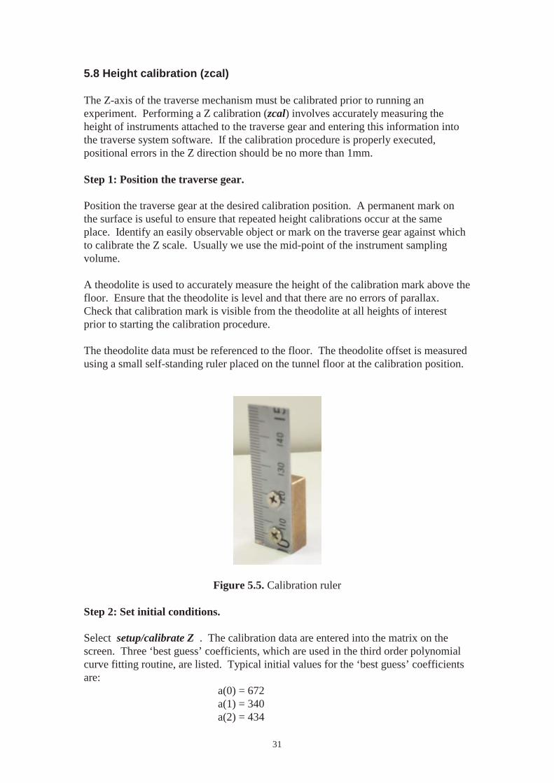
The theodolite data must be referenced to the floor. The theodolite offset is measuredusing a small self-standing ruler placed on the tunnel floor at the calibration position.
Figure 5.5. Calibration ruler
Step 2: Set initial conditions.
Select setup/calibrate Z . The calibration data are entered into the matrix on thescreen. Three ‘best guess’ coefficients, which are used in the third order polynomialcurve fitting routine, are listed. Typical initial values for the ‘best guess’ coefficientsare:
a(0) = 672a(1) = 340a(2) = 434

32
Step 3: Move the traverse gear to a new position.
Select Joystick option and click on the first cell under Counts. Move the traversegear to the required height using the joystick. Select OK or press Enter. Click onthe associated cell under Real(mm) and enter the actual height as determined by thetheodolite. Select OK.
Step 4: Move through the desired range in height.
Repeat Step 3 until the first four positions have been entered into the matrix. Click onCalculate to get new values for a(1), a(2) and a(3). Enter these estimates into the‘best guess’ positions. Repeat the above procedure after 8 positions and then again atthe end.
The recalculation of 'best guess' estimates during the zcal is an effort to prevent a fatal‘divide by zero’ error. This error appears to be random but may also be related tocertain mechanical configurations of the traverse gear.
Step 5: Get final calibration coefficients.
When all positions have been filled, select Calculate. The final calibrationcoefficients are listed. The Error Column in the matrix lists differences betweenactual height and calculated height. These differences should be less than 1mm. Ifthe calibration is unsatisfactory, it may be necessary to alter the configuration of theprobes on the traverse gear and to repeat the calibration.
The curve fitting routine uses a third order polynomial. It is worth plotting thecalibration equation over the height range of most interest in the experiment to ensurethat estimated Vs actual heights are indeed within 1mm at heights not included in thecalibration data set.

33
6. Signal conditioning system
Hot and cold wire output voltages are fed through a Signal Conditioning Systemaffectionately known as ANNIE. ANNIE consists of eight signal conditioners andthree bridge amplifiers. The Signal Conditioner is used to offset, amplify and filterthe signal so that it lies within an acceptable range of amplitude and bandwidth. Dailymeasurement of gain and offset for each ANNIE channel provides a measure ofamplifier and instrument performance and stability. These data are also required inhotwire and pressure transducer calibration and processing.
The following discussion assumes that the signals have been set up correctly. Seesection 3.4 for details of suggested record keeping.
6.1 Measuring gain
Signal gain is measured using a stable precision voltage source and a DigitalVoltmeter (DVM). (Suitable instruments are a YEW DC VOLTAGE CURRENTSTANDARD TYPE 2853 and a KEITHLEY 192 PROGRAMMABLE DMM.) Forgain settings of 10 or less, the voltage standard output is set to 1.000 volts. Gainsettings greater than 10 require that the reference input be reduced so that outputvoltage will be less than ± 12 volts. The digital voltmeter must have sufficientresolution to measure the Voltage Standard output to at least a millivolt. The inputvoltage is called Vin.
1. Switch the offset switches to OFF.
2. Ensure that the gain switch is located at the correct setting as determinedwhen the hot or cold wires were set up.
3. Measure and record the Voltage Standard output using the DVM. In mostapplications the gain setting is less than 10 and 1.000V can be used.
4. Connect the Voltage Standard output to the signal conditioner input andthe DVM that was used to measure the reference voltage to the signalconditioner output.
5. Record output voltage (V1) from the signal conditioner.
6. Swap the polarity of the reference input and record signal conditioneroutput (V2). Measuring the gain using both polarities eliminates anyresidual signal conditioner offset.
7. Signal conditioner gain can be calculate using:
( )inV
VVgain ×
+=
2
21
(6.1)

34
6.2 Measuring offset
1. Switch both OFFSET switches to ON and the gain switch to 1.
2. Connect a short circuit to the input of the signal conditioner.
3. Measure output voltage of the signal conditioner with a suitableDVM.
At the conclusion of the above measurements ensure that the gainswitch is set back to the required value, that the offset switches are setto ON or OFF as required and that the filter selection is at the correctcut off frequency. It is easy to record a large amount of useless data if
the switches are not left at the correct positions.
6.3 Signal conditioner frequency response
The filters used in ANNIE are Bessel type filters with typical response curves shownby Figure 6.1. This data can be used as a guide to select an appropriate filter settingfor each instrument. The choice of filter also depends on the frequency at which thesignal is sampled and whether aliasing effects are of concern. In most Pye LaboratoryWind Tunnel experiments, hot and cold wire data is sampled at 5000Hz. In the BlackForest Experiment, pressure transducer data were low pass filtered at 10Hz.
Typical Signal Conditioner Frequency Responseat each Filter Setting
0
0.1
0.2
0.3
0.4
0.5
0.6
0.7
0.8
0.9
1
10 100 1000 10000 100000
Frequency (Hz)
Am
plit
ud
ere
spo
nse
fo = 1KHz
fo = 2KHz
fo = 5KHz
fo = 10KHz
Figure 6.1. A typical signal conditioner frequency response with various cutofffrequency settings.

35
7. Data collection and logging systems
Data from hot and cold wires, pressure transducer, Vaisala temperature and roompressure are sampled and logged using an analogue data acquisition systemcomprising (Figure 7.1):
1. PC Curly; 486 PC running DOS applications.
2. Analog Devices RTI-860 16 bit Analogue to Digital Converter.
3. 16 way external input box to the Analogue to Digital Converter.
4. Various FORTRAN software to acquire data.
The Laser Doppler Velocimetry system consists of a TSI LDV system controlled byPC Larry. The LDV System uses it’s own logging system which is described insection 13 of this manual.
Figure 7.1. General layout of Data Sampling and Logging Systems.
7.1 Important logging system notes
1. Immediately after powering up PC Curly, run DMALOAD.EXE to configurethe analogue to digital converter. Failure to do so will result in Error 141.DMALOAD.EXE requires CONFIGB.DAT in the directory from whichDMALOAD.EXE is run. In most Pye Laboratory wind tunnel applications,DMALOAD.EXE is run from the current working directory.
2. PC Curly must not be run in ‘turbo’ mode when the RTI-860 analogue todigital converter is being used. The RTI-860 cannot sample fast enough whenthe controlling PC operates at the higher clock speed. Operation at the higherspeed causes corruption of collected data.

36
3. For all hardware and software details on the RTI-860 ADC, see the appropriateUser and Software manuals. These are located in the filing cabinet in the windtunnel room.
4. The Traverse Gear System PC Moe accepts RS232 inputs from the logging PCCurly and the LDV PC Larry. The source of RS232 inputs is set using aswitch box located on top of PC Moe. When sampling hot and cold wire data,the switch should be set to Curly. LDV measurements require that the switchbe set to Larry.
5. Data acquisition using the analogue to digital converter allows simultaneouscapture of four input channels. Simultaneous data capture is required toinvestigate second and higher order moments of turbulence signals. The RTI-860 allows simultaneous sampling of 2 groups of 4 channels. Channels 0through 3 constitute Group 1 and channels 4 through 7 constitute Group 2.Ensure that signals that need to be simultaneously sampled are connected tochannels in the same Group. The number of groups sampled (1 or 2) must becorrectly entered into input files XCAL.INP and PLANE.INP. See the RTImanual for complete details of groups and channels.

37
8. Using cold wire temperature sensors
Heat is often used in the Pye Laboratory wind tunnel as a passive scalar, so accuratemeasurements of temperature is necessary. In scalar transfer experiments accuracy’sof better than 0.1o are required. Careful calibration and operation of the cold wiresensors can achieve this. The following section describes the calibration proceduredeveloped during the Black Forest Experiment to provide high quality temperaturedata.
8.1 Cold wire resistance measurement
The resistance of the cold wire must be measured at room temperature prior tocalibration to determine the endpoints of the calibration. Be careful to select anOhmmeter that does not cause the wire to heat, as this will give erroneous results.Fluke 79 series digital multi-meters have been found to cause minimal internal heatingof the wire. Record the wire resistance as well as the temperature at which theresistance was measured. Most cold wires used in the Pye Laboratory Wind Tunnelhave a resistance in the range of 60 to 120Ω at room temperature. To a certain extent,locally hand made cold wires can have their resistance tailored to any reasonableresistance.
Wire resistance provides an idea of wire sensitivity. Wires with resistances lowerthan 60Ω are insensitive to turbulent heat fluctuations, whereas wires with resistancesgreater than 120Ω are fragile and easily broken. Higher resistance wires have a thinnerand or longer active region and are therefore more sensitive than shorter or thickerwires.
8.2 Calculating sensor end points
The resistance of a conductor (assuming a linear temperature coefficient) at anytemperature can be calculated from:
tmmt RRR ∆+= α (8.1)
where Rt = resistance at temperature t (Ω)Rm = resistance measured at temperature m (usually room
temperature)α = temperature coefficient of resistance∆t = t - m
Equation (8.1) is used to determine the calibration end points for cold wire calibration.Let Tcold be several degrees cooler than ambient temperature and Thot be severaldegrees higher than the maximum temperature likely to be measured during theexperiment. Then:
α = 0.0035 for platinumm = Room temperature = 20oCTcold = 15oCThot = 35oC

38
Rm = 80Ω at room temperature
Calculate from Equation (8.1):Rcold = 78.6ΩRhot = 84.2Ω
Rhot and Rcold are used to set the bridge amplifier on ANNIE using a decade resistancebox to simulate the resistance of the cold wire at various temperatures.
8.3 Signal conditioner settings
The cold wire signal is fed through a bridge amplifier and then through the signalconditioner. The bridge amplifiers are located to the right hand side of ANNIE. Boththe signal conditioner channel and bridge amplifier channel on ANNIE have GAINand OFFSET controls, however only the offset on the bridge amplifier is used.Obtaining a temperature signal is an art made a little easier by following these steps:
1. Signal conditioner: Cold wire signals do not use the Offset option. Select again of 10 and turn the offset switches OFF. Filter cut-off frequency shouldbe selected to give the maximum required frequency response relative tosampling frequency and aliasing problems. Most heat flux experiments thusfar conducted in the Pye Laboratory Wind Tunnel have used a filter cut-offfrequency of 5kHz where sampling occurred at 5kHz and the maximumfrequency response required was of order 500-1000Hz.
2. Bridge amplifier: Cold wire signals do not use the gain or filter option on thebridge amplifier. Set gain switch to 1 and switch the filter switch OFF.Measure bridge excitation voltage on the front panel of the amplifier andadjust bridge excitation to maximum (~ 13 volts). Turn offset to mid range (~5 turns). Turn fine and coarse balance controls fully anticlockwise
3. Connect an oscilloscope to the output of the bridge Amplifier. Theoscilloscope should be DC coupled and set to 5 volts/division. Connect adecade resistance box to the input of the bridge amplifier and set it to Rm (ascalculated in Section 8.2). The voltage on the oscilloscope should be ataround –10 volts. Slowly adjust the coarse balance control until the cold wireoutput voltage increases approximately –2 volts. Adjust the voltage to –2volts using the fine balance control.
4. Disconnect the oscilloscope from the bridge amplifier output and connect thebridge amplifier output to the input of a signal conditioner amplifier. Connectthe oscilloscope to the output of the signal conditioner amplifier. Adjust thefine balance control (and coarse control too if necessary) on the bridgeamplifier to bring the voltage shown on the oscilloscope back to –2 volts.
5. Switch the decade box to Rcold. Check that the cold wire output trace on theoscilloscope does not exceed +5 volts. Switch the decade box to Rhot. Checkthat the trace does not go below –5 volts. The oscilloscope sensitivity shouldbe increased to ensure that the signal stays within the ±5V range. A digitalvoltmeter can be used to achieve the same goal. The signal must not exceed +5

39
or – 5 volts over the temperature range measured in the wind tunnel. Theinput range of the analogue to digital converter is ±5 volts so any data outsideof this range is not recorded. If the voltage from the signal conditioner exceeds±5 volts the range can be reduced by either decreasing the bridge excitationvoltage or reducing the signal conditioner gain.
6. Record the voltage range so that the resolution of the temperature data can bedetermined.
The cold wire should now be operational with sensitivity sufficient for the experimentat hand. Placing the probe over a beaker of hot water can test the operation of the coldwire. The trace on the oscilloscope should resemble that of a turbulent signal.Traverse the probe slowly away from the top of the beaker. The signal on theoscilloscope should show lower amplitude and frequency until no signal is evident.The cold wire is now ready to be calibrated.
Figure 8.1. Bridge amplifiers for cold wire sensors (two RHS modules) alongsidesignal conditioner amplifiers (LHS modules), collectively known as ANNIE.
8.4 Setting up the temperature controlled calibration box
When the bridge amplifier and signal conditioner have been set up, the sensor can beplaced in the temperature controlled calibration box. The temperature inside thecalibration box is controlled over a range of temperatures by a Peltier cell andelectronic feedback control system. Temperature stability of ±0.03o can be easilyachieved. Two small high-speed fans mounted on each side of the calibration area mixthe air inside the box.

40
The cold wire is calibrated in the probe mount that is attached to the traverse gear (seeFigure 8.5) to ensure that calibration occurs under the same configuration as datameasurement. The cold wire is mounted in the calibration space between the two fansand is closely flanked by the temperature controller sensor and a precisionthermometer (THERMOMETRICS TS8901). Be sure to seal the box carefully so asnot to break the cold wire. The cold wire is very vulnerable during temperaturecalibration. If the box is placed over heated panels it should be lifted a fewcentimetres off the floor, otherwise it may be difficult to get the box to temperatureslower than ambient. The gap around the traverse gear and the box should be filledwith tissues so that the exchange of air between the inside of the box and the externalenvironment is reduced
Temperature controller schematics are shown in Figure 8.4. The set temperature isdisplayed on a digital voltmeter. The temperature controller is calibrated in degreesKelvin so that 3.00 volts is equal to 300oK. Another set of terminals on the frontpanel of the temperature controller box allows internal box temperature to bedisplayed. Swapping terminals to the digital voltmeter allows one to monitor thetemperature controlling process and make a decision regarding stability of the system.The Calibration Box takes approximately 10 minutes to equilibrate after the set pointhas been changed.
Figure 8.2. Temperature calibration controller.
Ensure that hot wire anemometers are switched off if they areadjacent to cold wire sensors that are undergoing calibration.
Otherwise gusts of hot air from the hot wires affect thecalibration results.

41
Figure 8.3. Temperature controlled calibration box.
Figure 8.4. Schematic of temperature calibration box and feedback mechanisms.

42
Figure 8.5. Layout of temperature sensors inside the calibration box duringcalibration.
8.5 Cold wire calibration
The temperature coefficient, α (see Equation 8.1), for platinum is essentially linearover the expected temperature range in the Pye Laboratory Wind Tunnel (-5 to 40oC)so that the relationship between cold wire output voltage and temperature is a straightline in our circumstances (Lomas 1986:37).
Although three calibration points should be sufficient to determine the regressionequation, it is wise to extend the calibration to five points to allow for experimentalerror. Each calibration temperature should be separated by 2 or 3o and should span thefull range of expected temperatures. Temperature calibration is a time consumingprocess, so allow at least four hours for a standard five-point calibration.
It takes approximately 10 minutes for the temperature of the calibration box tostabilise after setting a new temperature (Figure 8.6). If the incremental temperaturechange is small, the stabilisation time will decrease. Stability time is similar whenadjusting the temperature up or down.
The temperature of the calibration box is measured using a THERMOMETRICSTS8901 precision thermometer and the data are logged by BOX_TEMP.WK1 runningunder Lotus Measure. The precision thermometer is connected to the logging PC viaa GPIB interface. The data from the precision thermometer can also be manuallyrecorded. Cold wire data are collected via ANNIE and the analogue to digitalconverter through TCAL.EXE which runs on PC Curly (Section 8.6). This programcan record multiple inputs and produces an ASCII file of time, mean voltages andstandard deviations. Since two independent computer systems collect data from twoinstruments with very different response times, it is important that the temperature in

43
the calibration box be stable when data logging is commenced and that the clocks ofthe computers are synchronised. It is useful to ensure that the PC’s used to logtemperature data are synchronised to common time reference.
Temperature Time Series
28
29
30
31
32
33
34
35
36
37
38
11:4
0
11:4
2
11:4
4
11:4
6
11:4
8
11:5
0
11:5
2
11:5
4
11:5
6
11:5
8
12:0
0
Time
Tem
per
atu
re(C
)
Figure 8.6. Typical temperature trace after changing the set temperature in thecalibration box.
8.6 Using TCAL.EXE
TCAL.EXE acts as a sampling voltmeter by recording the mean and standarddeviation of 5000 voltage samples every minute. Up to eight channels can berecorded simultaneously. TCAL.EXE is primarily used for temperature calibration.The temperature sensor signals are fed through the bridge amplifier and signalconditioner to the analogue to digital converter and PC Curly. Input questionsinclude:
1. Calibration number: a sequence number or some value corresponding to thecurrent temperature set point.
2. Number of channels to log: number of sensors being calibrated. Usually 1 or2 channels are used for a standard cold wire calibration.
3. ADC channel used: analogue to digital converter channel numbers to whichthe cold wires or other temperature sensors are connected.
4. Type of sensors connected to each input channel: sensor numbers are 3 forthermistor beads and 4 for cold wires. The sensor type number is not used byTCAL.exe, but in the processing programs only, hence the number can be anyvalue if the data is not used by PROCESS.EXE

44
5. Number of minutes to log: Make this as long as required. For mostapplications 20 minutes per temperature is sufficient as long as thetemperature of the calibration box has already stabilised.
The output data from TCAL.EXE are saved in ASCII format as TCAL???.DAT where??? is the sequence number given in Step 1 above. It is sensible to run TCAL.EXEindependently for each new temperature setting after the Calibration Box has reachedtemperature equilibrium. Multiple runs have the advantage of labelling the output filesaccording to expected box temperature which makes later analysis more selfexplanatory.
The voltage data in TCAL???.DAT are regressed against precision temperature datacollected in Lotus Measure (See section 8.5) to determine a calibration equation forthe sensor of interest. The response times of the cold wire and precision thermometerare quite different as the data recorded by TCAL.EXE is an average of 5000 readingsand the data from the precision thermometer is a single reading. Thus it is importantthat only those data representative of stable temperature conditions in the calibrationbox be used in the regression. An example of a typical calibration run is shown inFigures 8.7 and 8.8. Note that in runs 1, 3 and 5, the temperature in the calibrationbox had not reached equilibrium prior to starting TCAL.EXE as evidenced by thefluctuations on the cold wire trace. The first couple of minutes of data should bediscarded from the calibration regression for these runs.
The results from the regression are input into the appropriate calibration file. For acold wire, the calibration file is called CWI???.CAL. An example of file content islisted in Table 8.1. The calibration number is manually input into PLANE.INP andautomatically input into PROCESS.INP for later reference during data processing.
Table 8.1. Example of a cold wire calibration file. Regression coefficients match thecalibration run shown in Figures 8.7 and 8.8.
Calibration information for TT4 cold wire obtained by calibration Day 218(6 Aug, 1998)
-----------------------------------------------------------------------------------------------------Coefficients of a straight line are:
32.132 a0-8.0351 a10.0000 a2

45
Cold wire time series
-0.5
0
0.5
1
1.5
2
12:5
0:00
13:0
0:00
13:1
0:00
13:2
8:00
13:3
8:00
14:0
5:00
14:1
5:00
14:4
6:00
14:5
6:00
15:2
2:00
15:3
2:00
16:0
0:00
16:1
0:00
16:2
0:00
16:5
1:00
17:0
1:00
Tim e
Co
ldw
ire
volt
age
Figure 8.7. Cold wire output voltages for seven calibration temperatures. The datafor each temperature were recorded in a different TCAL???.DAT file.
Coldwire voltage Vs Temperature
y = -8.0351x + 32.132R2 = 1
15
20
25
30
35
40
-0.5 0 0.5 1 1.5 2
Cold wire Voltage
Tem
per
atu
re
Figure 8.8. Regression of temperature calibration data.

46
8.7 Notes on the use of cold wire temperature sensors
1. Cold wire sensors are fragile and subject to a number of problems. The mostobvious is total failure due to wire fracture. It is useful to monitor outputvoltage so that failure can be quickly identified. It is quite possible to record alot of useless data if this step is not taken.
2. Dust and other airborne substances quickly contaminate cold wire sensors.Severe contamination causes the frequency response of the wire to be greatlycompromised and the effect is clearly visible on an oscilloscope. A moresubtle effect is shifting of the calibration as wire characteristics change. Wefound that the fog used by the laser Doppler system contaminated a cold wirewithin 30 seconds of exposure in the free stream. A more disturbing resultwas the tendency for a cold wire to be contaminated in experiments runimmediately after use of the laser Doppler system. The Rosco fog fluidappears to persist in the tunnel for many weeks after use, the implication beingthat deposited droplets slowly volatilise back into the tunnel atmosphere.Although carefully dipping it in warm soapy water and then flushing it withdistilled water can clean a cold wire, it is better not to allow contamination inthe first place. The wire often breaks during cleaning and if it survives,complete re-calibration is in order as the wire has been mechanicallydisturbed.
3. It is good practice to measure cold wire resistance before each day ofexperiments. We have measured sudden shifts in cold wire resistance fromone day to the next. The cause of these shifts is not known but the outcome isa shift in the intercept of the regression. We took to performing a one-pointcalibration each day of experiments to ensure that the calibration coefficientswere updated on a regular basis.
4. The signal from the cold wire can be contaminated by bursts of hot air blownover from adjacent hotwire probes. Calibration of cold wires should occurwith the hotwires off. Contamination of temperature data from a cold wire co-located with hotwires will occur in any turbulent flow that has lateral and flowreversal components. Although contamination can be minimised by placingthe cold wire slightly in front of the hotwires and offset to the side, thecompromise is increased sampling volume. It is common practise in thesecircumstances to repeat profiles with the hotwires off so that at least a reliablemean temperature and standard deviation can be obtained. However, heat fluxand higher order moment’s uiujt will probably be overestimated.
5. Long term stability of the complete cold wire measurement chain (probe andamplifier) has been found to be approximately to be 0.1oC over a period of 10days. The drift appears to be due to mechanical changes in the sensor wireitself and electrical drift in the amplifiers.

47
8.8 One point temperature calibration
One point temperature calibration is a convenient way of checking the operation of acold wire sensor. The procedure should be used regularly to check that the cold wire isfunctional and that no significant calibration drift has occurred.
Move the traverse gear so that the cold wire (or other temperature sensor) is in the freestream. Place the precision thermometer sensor as close as possible (but not touching)to the cold wire. Run the logging programs for about 30 minutes. The averagetemperature recorded by both devices should be very similar. If there is a significantdifference between the readings then a complete re-calibration will be required.

48
9. Pressure measurements
The Pye Laboratory Wind Tunnel is equipped with several instruments for measuringdynamic and static pressure to determine wind speed, pressure changes down thetunnel and pressure drop across the contraction. Two devices are provided for pressuremeasurements, these being an electronic differential pressure transducer and a watermanometer.
The output from the electronic pressure transducer can be amplified and filtered asrequired by using a signal conditioner amplifier. The water column provides a usefulstandard against which to compare the pressure transducer.
To make the use of the pressure transducer more versatile, the transducer is mountedinside an enclosure which also contains four solenoid valves that allow the inputs ofthe pressure transducer to be ‘shorted’ or switched between two different pressuresources. Shorting the transducer input allows the offset voltage of the pressuretransducer and associated amplifier to be measured. This is required so that we candetermine what the output voltage is for a zero pressure differential input. The valvesdefault to input 1 as shown on the transducer enclosure.
Remote switching (i.e. controlled by PC Curly) of the valves is performed via the vanecontrol interface box. Two outputs are provided to either select the ‘short’ position orto select the required input position. The valves can also be switched manually bymeans of switches on the front panel of the transducer enclosure. In this case the‘Auto/Manual’ switch should be in the ‘Manual’ position and the valves switched asrequired. The ‘Auto’ position is selected when the PC is to control the valves.Indicator LEDS show the current state of the valves.
For maximum stability of the pressure transducer, it should be leftpowered continuously. The enclosure should be left closed as this
improves the thermal stability of the transducer.
Before using the water manometer ensure that:
1. There is sufficient water level in the instrument. Fill with distilled water and adrop of surfactant. (Dishwashing liquid is suitable for this purpose)
2. Check the bubble level on top of the instrument to ensure the instrument islevel.
3. The instrument reads zero when its pressure ports are joined together. Adjustthe scale position by means of the knurled knob on the top of the instrument ifrequired.

49
The water manometer display is calibrated in Pascal not mm of water! (See themanometer manual for details.) Note also that the calibration is exact only for the20oC, however the error is small and can usually be neglected. See the instrumentmanual for details.
Calibration of the pressure transducer should be performed at the commencement ofan experiment. This is easily done using the program COMPPRES.EXE.
Figure 9.1. Pressure transducer enclosure (centre) and water manometer (right).
Transducer
+
-
Input #1+
Input #2 -
#2 +
#1 -
Short
Figure 9.2. Schematic of pressure transducer plumbing inside the transducerenclosure.

50
10. Setting the roof profile
10.1 Pressure differential and the Navier Stokes equation
The first priority of a boundary layer wind tunnel is to produce steady and uniform air-flow into the working section. Once in the working section, the fate of the mean andturbulent flow can be described by the Navier Stokes equation for motion:
In the Pye Laboratory wind tunnel, the flow is steady and Coriolis ( fcΣij3) andbuoyancy (δi3g) terms can be neglected. The viscous terms are small compared withthe turbulent terms can also be neglected. The Navier Stokes equation thus becomes:
x
’u’u
x
P1-=
xU
Uj
ji
ij
ij ∂
∂−
∂∂
∂∂
ρ(10.2)
In the free stream, the turbulent terms are negligible thus we get:
x
P1-=
xU
Uij
ij ∂
∂∂∂
ρ(10.3)
Integrating both sides, we get Bernoulli’s Principle
constant=gzP+U21
j2 +∫ρ (10.4)
In a wind tunnel environment gz is constant and can be rolled into the term on theright hand side of equation 10.4. The first term represents dynamic pressure, whichideally should remain constant throughout the tunnel because the flow is supposed to
be steady without dynamical effects. Thus static pressure P must be constant throughthe length of the tunnel and dP/dx = 0. It follows then that in turbulent flow that issteady without dynamical effects,
x
’u’u
x
U+
x
P1-Uf+g=
xU
U+tU
j
ji
2j
j2
ij3jic3i
j
ij
j
∂∂
−∂∂
∂∂−
∂∂
∂∂
νρ
εδ (10.1)

51
x
’u’u=
xU
Uj
ji
j
ij ∂
∂−
∂∂
(10.5)
which implies that any divergence of flux will manifest itself in an acceleration ordeceleration of mean wind speed, thereby greatly simplifying experimental procedureand data interpretation.
Controlling static pressure fluctuations is achieved via a flexible roof in the workingsection of the wind tunnel. Since tunnel air is not mixed with outside air in theworking section, the ability to adjust the roof height provides a great range of controlallowing both favourable and adverse pressure gradients to be readily obtained. Staticpressure differences should be checked at the beginning of each experiment andwhenever the physical or thermal environment of the tunnel change.
In the Pye Laboratory wind tunnel we aim to reduce the differential along the tunnel toa level that will not affect the experimental results. A suitable value has been found tobe 1%, or less, of the maximum dynamic pressure that is measured by a Pitot Statictube subjected to the maximum wind speed of the experiment. For instance, if thepressure measured by the Pitot Static tube is 80Pa, then the maximum pressuredifferential should be no more than ±0.8Pa. This pressure difference should bemaintained for 4 or 5m upwind of where the measurements are to be made.
10.2 Adjusting the tunnel roof
The tunnel roof is adjustable by means of handles located on the side of the tunnelclosest to the door side of the tunnel room. The roof can be moved up and down insegments of around 1-2m in length. The aim is to adjust the roof so that the pressuredifferential is minimised whilst maintaining a smooth roofline.
Before attempting to measure or adjust the pressure differential, it isimportant to move the traverse gear to a position as close to the open
end of the tunnel as possible. Also ensure that all tunnel accesswindows are closed and experimental conditions prevail.
The pressure differential is measured between pressure ports located along the tunnel.There are 14 ports in total. The first decision to make is where the experiment is to beperformed. This is required so that the reference port can be selected. For example, ifthe experiment were to be performed towards the end of the tunnel, between positions9 and 11 say, then port 10 would be the reference port. The pressure transducernegative input is connected to the reference port. The positive input to the pressuretransducer is then connected to the other ports as required.

52
Figure 10.1. Tunnel wall pressure ports.
To aid the setting of the roof, a program PSURVEY.EXE is provided on PC Curly.This program reads the pressure transducer, prompts the user to change ports asrequired and then displays the results. Psurvey.exe requires some details to beprovided in a file PSURVEY.INP. This file provides the set up details forPSURVEY.EXE.
Table 10.1 Contents of a typical PSURVEY.INP file:
Psurvey initialisation file: PVfact, input channel, Amplifier Gain9.9160710.599
The first entry is the sensitivity of the pressure transducer (also known as Pvfact invarious other programs) in mV/Pa. The second entry is the ADC input channel, thelast entry is the gain of the signal conditioner that the pressure transducer is connectedto. If no signal conditioner is used then this entry should be 1.0
If the roof requires significant adjustment, it is best to start with the ports closest tothe reference port and work out from there. In this case, ignore the prompts ofpsurvey.exe and repeat the measurement at the same port until the pressure differentialis as required. This is an iterative process and it may take some time to get it correct.

53
Figure 10.2. Adjusting the flexible roof.
Once the roof has been adjusted to the correct shape, psurvey.exe can be run throughcompletely. This generates a data file, PSURVEY.DAT.
Table 10.2 Contents of a typical PSURVEY.DAT file:
8.600000E-01 20.5580501.770000 3.1098402.685000 -7.549684E-023.660000 -9.872510E-024.515000 -7.404421E-025.435000 -4.500850E-026.345000 2.177717E-027.285000 -8.856283E-029.100000 -7.404421E-0212.785000 3.484316E-0213.690000 -3.27535114.600000 -2.49861715.520000 -2.932717
The first column is the distance from the start of the tunnel, the second is the pressure(in Pa) with respect to the reference port. We are generally only interested in the partof the tunnel where measurements occur. Figure 10.3 shows the above data plotted:

54
P r e s s u r e V s P o r tP o r t
- 5 . 0 0 E - 0 1
- 4 . 0 0 E - 0 1
- 3 . 0 0 E - 0 1
- 2 . 0 0 E - 0 1
- 1 . 0 0 E - 0 1
0 . 0 0 E + 0 0
1 . 0 0 E - 0 1
2 . 0 0 E - 0 1
3 . 0 0 E - 0 1
4 . 0 0 E - 0 1
5 . 0 0 E - 0 1
2 3 4 5 6 7 8 9 1 0 1 1 1 2
P o r t
P a
Figure 10.3. Typical port pressures along the tunnel.
The roof adjustment is acceptable if the pressure differential is below the 1% of thefree stream dynamic pressure. Note that the run-to-run variability in the measurementis approximately ±0.1Pa, so little is gained by attempting to reduce the differential toless than ±0.1Pa. At this stage the roofline should be viewed. It should be a smoothcurve without any significant bumps. If there are bumps, repeat the adjustment toobtain a smooth roofline.

55
11. Wind speed measurement using pressure
11.1 Bernoulli’s Equation
Recalling eqn (10.4), Bernoulli's equation for steady isentropic flow is:
This may be written as:
Integration of this equation and assuming constant density (i.e. incompressible flow),Bernoulli's equation reduces to:
Where H = total head,P = static pressure
U = wind speed
11.2 Measurement of total head H
The velocity at the nose of a bluff body placed in the fluid stream is zero, and so thepressure at this point is by definition the stagnation pressure. A stagnation pressure isnot determined uniquely by the undisturbed conditions of the fluid, but is associatedwith an arbitrary type of deceleration or recompression. However, provided that thevelocity of the undisturbed flow is subsonic, there is considerable evidence thatsuggests that the stagnation pressure at the nose of a body is very closely equal to thetotal head (H) in the stream tube leading to the stagnation point. This fact is exploitedin the measurement of the total head by the instrument usually referred to as the Pitottube, named after Henry Pitot (1695-1771) who measured the velocity of the RiverSeine using a narrow bent tube. A Pitot tube consists essentially of an open-mouthedtube placed with its axis along the direction of flow and with the open end facingupwind.
A Pitot tube works in the following way: Consider two points 1 and 2 at the samelevel, point 1 being away from the tube and point 2 being immediately in front of theopen end where the fluid velocity is zero. Friction is negligible along a streamlinethrough 1 and 2, so that Bernoulli's equation gives
linestreamalongconstant=zg+dp
+U2
1 2
ρ∫ (11.1)
0=dUU+dp
ρ(11.2)
U2
1=p-H 2ρ (11.3)

56
from which velocity is found as
Pressures at the two points are found from the hydrostatic balanceSo that velocity can be found from
)h-h(g2=U 121 (11.7)
Note that in terms of our earlier definitions, p2 is the stagnation pressure and is larger
than the local static pressure. Stagnation pressure is thus the sum of dynamic (2
2Uρ
)
and static (p) pressures.
ρρρp
=2
U+p
=2
U+p 22
221
21 (11.4)
ρ)p-p(2
=U12
1 (11.5)
hg=p ii ρ (11.6)

57
11.3 Measurement of static pressure
Since the static pressure is constant across the cross section, it can be measured at asolid wall along which the fluid flows. This approach is often desirable, as it is notnecessary to introduce a foreign object into the flow. A small hole is drilled in thewall at the point where the static pressure is to be measured, of diameter about 0.5mm. The fluid flows past the hole but remains at rest in the hole itself if itsdimensions are sufficiently small. The fact that the velocity is different outside andinside the hole is not in contradiction to Bernoulli's equation, since the Bernoulliconstant for the two regions is different (Prandl and Tietjens, 1934).
Owing to the influence of viscosity there is some sucking action which becomessmaller with decreasing hole diameter. Given a hole of diameter around 0.7 mm, theactual pressure exceeds the measured pressure by about 1%. In other words, p0
denotes the actual pressure, p1 the measured pressure, and U the velocity of the fluidflowing along the hole, we have:
It seems to be important that the flow is not disturbed at the point where the staticpressure is measured. For instance, it is necessary to make sure that no burrs exist atthe mouth of the hole. Small inaccuracies in this respect lead to completely falseresults (Prandl and Tietjens, 1934)
Figure 11.1 A Pitot Static (From Goldstein )
2
U0.01+p=p 10
2ρ
(11.8)

58
11.4 Velocity measurement using a Pitot Static tube
The measurement of the total head, H, and the static pressure, p, can be carriedsimultaneously using a Pitot Static tube (figure 11.1). In this case the stagnationpressure is measured at the tip of the tube and the static pressure is measured by holeplaced tangentially around the tube at a distance downwind from the nose of the tube.The use of a differential pressure transducer allows us to directly measure the pressure
difference, H – p. Thus U is determined using:
ρP
U2= (11.9)
where U = local wind speed (mS-1)P = pressure measured by Pitot Static tube (Pa)ρ = air density ( kgm-3)
Air density can be calculated from the air pressure and temperature using:
( )T
Pmm
+=
16.273
46465.0ρ (11.10)
or
( )T
PPa
+=
16.273
3486.0ρ (11.11)
where Pmm = Atmospheric pressure in mm HgPPa = Atmospheric pressure in hPaT = air temperature in degrees Celsius

59
11.5 Measurement errors
It is very important when using a Pitot Static tube to measure wind speed that the noseof the tube is straight into the wind. The angular deviation from this position is knownas the yaw angle. Should the yaw angle not be zero, the measured pressure will be
lower than expected, resulting in an incorrect speed measurement. Errors of 5% in Ucan be expected if the yaw angle of the Pitot Static tube is 15o. It is good practice touse a small spirit level to set the tube to horizontal and to sight down the tunnel toensure that it faces directly into the wind. If desired, it is possible to place weightedstrings in front and behind the tube to line the tube up with the long axis of the tunnel.In practise, however, the zero-yaw position of the Pitot tube head corresponds to themaximum measured pressure, so the tube can be aligned until this maximum isreached (Pankhurst and Holder, 1952:180-181).
Also see Goldstein 1983:Section 3.3 ‘Physical Errors in the Measurement of SteadyPressures’, for a detailed account of errors when using Pitot Static tubes to measurewind speed.

60
11.6 Using throat pressure for velocity measurements
For many experiments it is inconvenient to have a Pitot Static tube mountedpermanently in the tunnel. In this case it is possible to calibrate the pressure dropacross the tunnel contraction against wind speed at the desired measurement position.This cross calibration should be done AFTER the roof has been adjusted. Theadvantage of using throat pressure drop to determine wind speed at a point is that thecalibration relationship is independent of local temperature and pressure conditions,assuming no change in the physical characteristics of the tunnel, i.e., the roof is notchanged and calibration occurred once the tunnel had come to thermal equilibrium.
The program COMPPRES.EXE is very useful for this procedure as it steps the tunnelthrough 16 different wind speeds and records the Pitot Static pressure and throatpressure at each speed. Each pressure can then be converted to an equivalent windspeed and the relationship between the two values can be determined. Alternatively,the water manometer may be used to measure the Pitot Static pressure, which is thencompared with the throat pressure measured by the pressure transducer.
COMPPRES.EXE requires the following plumbing to be set up:
Tra
nsdu
cer
+
-
Transducer enclosure
To throat pressure ports
Wat
erM
anom
eter
#1+
#2+
#1-
#2-
To PitotStatic tube
Figure 11.2. Plumbing for calibrating the pressure transducer and throat pressure.
Using the above set up allows you to calibrate the pressure transducer as well asdetermine the Pitot Vs throat pressure relationship. Typical results from the above setup are:

61
Table 11.1. Transducer and throat pressure calibration.
Pitot Vs throat calibration data file-------Date of calibration :18-05-1998Time of calibration :10:13Calibration number :001Temperature (deg c) 24.3Pressure (mm Hg) 717.4Offset voltage (mV) : -48.115Amplifier gain : 1Speed# Ufree Pitot(Pa) Pitot(mV) Throat(Pa) Throat(mV) Manometer (pa) Pitot(mV)
1 1.421 1.133 11.34 -1.347 -13.481 0.9 11.342 1.29 0.934 9.349 -1.253 -12.541 1 9.3493 1.818 1.855 18.577 -0.549 -5.501 2 18.5774 3.067 5.278 52.84 1.907 19.095 5.5 52.845 4.023 9.082 90.927 4.497 45.028 9.5 90.9276 5.019 14.133 141.497 7.946 79.558 14.6 141.4977 6.055 20.573 205.981 12.414 124.286 21.2 205.9818 6.943 27.044 270.764 16.863 168.828 27.7 270.7649 7.758 33.769 338.099 21.426 214.518 34.5 338.099
10 8.569 41.196 412.456 26.553 265.846 41.7 412.45611 9.142 46.891 469.475 30.265 303.008 47.5 469.47512 9.814 54.042 541.071 35.289 353.309 54.8 541.07113 10.417 60.879 609.522 39.92 399.678 61.8 609.52214 11.266 71.214 712.993 47.284 473.408 72 712.99315 11.775 77.8 778.93 51.447 515.092 78.7 778.9316 12.02 81.063 811.599 53.494 535.584 81.8 811.599
Transducer Calibration: 18 May 1998:Day 138
y = 9.9177x - 1.9311R2 = 1
0
100
200
300
400
500
600
700
800
900
0 20 40 60 80 100
Pressure Input (Pa)
Tra
nsd
uce
rO
utp
ut
(mV
)
Throat Vs Pitot Pressure
y = 1.4587x + 2.6222
R2 = 0.9999
0
10
20
30
40
50
60
70
80
90
-10 0 10 20 30 40 50 60
Throat Pressure (Pa)
Pit
ot
Pre
ssu
re(
Pa)
From the above it is easy to determine the relationship between the velocity measuredby a Pitot Static and the throat pressure. This is useful as it allows the equivalent windspeed to be logged without having a Pitot Static tube mounted permanently in thetunnel.

62
12. Calibration of hot wire anemometers
Accurate and reproducible calibration of hot wire anemometers is critical to thesuccess of any experiment that uses them. The user needs to have a goodunderstanding of how they work and their limitations. The following pages describeboth general and specific points relating to the use of hot wires in the Pye LaboratoryWind tunnel. Setting up the hot wire bridge is well covered in the TSI bridge manualsand will not be repeated here.
The first part of this section will cover the conventions used and some backgroundinformation on the techniques used. Following this will be the detailed steps using theexisting hardware and software.
The system of logging and analysis that has evolved over time requires that certainconventions be adhered to. In particular this applies to the designation of wires in ‘X’and ‘triple’ wire probes. Failure to observe these conventions will result in erroneousdata. In particular, the direction of the wind may be 180 degrees out.
12.1 Wire designations
NOTE: z axis is vertical in the following 3 cases
wire 1 --------------------------// <------- wind direction
---------------------
wire 2 -----------------------\\ <------ wind direction
-------------------------
wire 3 ----------------------|| <------ wind direction
----------------------
The above wire geometry must correspond with particular input channels. i.e.
wire 1 wire 2 wire 3----------------------------------------------------
channel 0 or 3 1 or 4 2 or 6
See the RTI-860 ADC manual for complete details of the channels and groups that areallowed by the ADC hardware and software.

63
12.2 Wire uniformity
It has been found that the sensitivity of each anemometer in a group must be uniformfor best results. This is particularly true when correlation of a number of velocitychannels are required. This means that the output voltage of each anemometer shouldbe more or less the same for the same range of wind speeds. Commerciallymanufactured X wire probes are usually uniform, the real problem occurs whenmaking up probe assemblies with different hot wires. The best solution is to use thesignal conditioner Gain and Offset controls to match the voltages for each hot wire.Typically, the signals can be matched to better than 0.1 volts over a 4 volt range. Aniterative approach is required to set up the signals, the gain control being adjusted atmaximum wind speed and the offset control being adjusted at minimum wind speed asmany times as required to match the wires. If this signal matching is done, then besure to select the ‘measured voltage option (1)’ when XCAL_THR.EXE is run. Whenthis option is selected, the raw voltage is recorded rather than the voltage corrected foramplifier gain and offset. This is then taken into account when the data processing isundertaken.
12.3 Wire angle
The default X wire angles are +45.00o for wire 1, -45.00 o for wire 2 and 0.00 o forwire 3. A yaw calibration (yawcal) procedure can be undertaken to accurately measurethese angles. Whenever any change is made to an individual probe or probe assembly,the yaw calibration should be undertaken. It has been found that over time, wires willdeviate from the above default values by up to ± 3 o.
When the hot wires are installed in the tunnel in whatever probe assembly is used, it isimportant that the probes be accurately aligned with the axis of the tunnel. The probesshould be level and the wires should be completely contained within the measurementplane of interest. For instance, if the U and W velocity components are of interest, thehot wires should be completely in the x z plane.

64
12.4 General set up for hot wire calibration
When calibrating hot wires, a reference wind speed is required. This can be in theform of a Pitot Static tube or the related throat pressure. If a Pitot Static tube is usedthen the hot wires should be as close as possible to the Pitot Static tube. The followingfigure shows one possible configuration:
Figure 12.1. Hot wire calibration set up using a Pitot Static tube.
As mentioned previously, it may be more convenient not to use a Pitot Static tube, butto rely on the throat pressure. In this case it is very important that the Pitot/Throatrelationship be derived with the Pitot Static tube in the exact position where hot wirecalibrations are to take place.
The hot wires are best calibrated in a region where turbulence is low, this usuallymeans a position towards the fan end in the free stream, before the boundary layer hashad time to fully develop. Calibration should be done after the roof has been adjustedfor minimum pressure differential.
12.4.1 Wind speed calibration (xcal) procedure
Each hot wire anemometer needs to be calibrated so that we can determine itscalibration coefficients. We generate a set of coefficients that allow us to fit the hotwire function to Kings Law:
rnUBAV +=2
(12.1)
Where V = output voltage from a hot wire channel measured by the ADCA = zero velocity outputB = sensitivity of wire
U = mean wind speedrn = an exponent to make the expression linear.

65
NOTE: rn is approximately 0.45 if ‘measvolt’ = 0 when running XCAL_THR.EXErn is approximately 0.7 if ‘measvolt’ = 1 “The function of ‘measvolt’ is described in the following notes.
Running XCAL_THR.EXE allows us to determine the above coefficients. This isdone by running the tunnel through a range of 16 wind speeds, recording the hot wirevoltage at each speed, and then fitting the data to a suitable curve.
When a hot wire probe is first assembled a number of steps need to be undertaken:
1. Perform an xcal using default wire angles for each wire, i.e. set the wire anglesto ±45 o for x wires and 0o for normal wires in XCAL.INP
2. Measure the actual wire angle by selecting the yawcal option when runningXCAL_THR.EXE Note that a dummy XWI???.YAW file must be present forthis. The file just needs to exist, it doesn’t matter if it is not relevant to theprobes being used. The later yawcal will create a relevant file.
3. Perform another xcal using the new wire angles determined above tocompletely characterise the hot wire. The new wire angles must be entered intothe file XCAL.INP
4. If the wire has been used in its current configuration, only a single xcalprocedure is required. It is good practice to perform a complete sequencewhenever the probe assembly is moved or altered in any way.
Run XCAL_THR.EXE to start a xcal sequence. XCAL_THR asks a number ofquestions:
Calibration number: This number is a sequence number thattracks the calibration file through its use.The numbers are usually sequential forany particular probe assembly, starting at1 when the probe is first assembled.
Air temperature (C): Get this from the mercury thermometermounted on the side of the tunnel.
Air pressure (mmHg): Get this from the mercury barometerupstairs.
Use (1) Measured or (2) Bridge voltage: This sets the ‘measvolt’ flag thatdetermines whether the voltage measuredby the PC is corrected for the gain andoffset of the signal conditioner. If thewires are well matched in terms ofresistance then select ‘2’, if the wires are

66
not well matched in resistance then select‘1’. (See the comments of wireuniformity above) Selecting ‘1’ in eithercase will do no harm.
Use (1) Throat or (2) Pitot pressure: This determines what is used as thespeed reference for the calibrationsequence. If ‘2’ is selected, a Pitot Statictube is assumed and the wind speed iscalculated directly. If ‘1’ is selected, thenthe transfer function between the throatpressure and wind speed is invoked.
The offset voltage of the pressure transducer is then measured and displayed at thispoint.
Do you wish to perform a Yaw calibration (y/n)? Answer ‘n’ if running and xcal,‘y’ if doing a yawcal.
Assuming you answer ‘n’ to the above, then you are asked:
latest yaw calibration file no: Enter the sequence number of the lastyawcal file here. If this is the first xcal tobe performed, then you will need adummy XWI???.YAW file to be present.See the comments above. xcal will fail ifthe specified file is not present.
Do you wish to perform a normal Answer ‘y’ here to continue thecalibration (y/n)? sequence, ‘n’ will terminate the program
operation.
If the ‘Auto Traverse’ option has been set in XCAL.INP, the probes will now move totheir calibration position and the tunnel will automatically run through a range of 16speeds, the hot wire output being recorded at each speed. At the conclusion of theprogram a file XWI???.CAL will have been created (??? is the sequence numbergiven at the beginning). The XWI???.CAL file will contain the wind speeds measuredat each setting, the corresponding hot wire voltages and the calculated coefficients tofit the data to Kings law.
If the ‘Auto Traverse’ option has not been set, then you will be asked to manuallymove the traverse gear to the correct calibration position before continuing with thecalibration sequence as above.

67
Table 12.1. The contents of a typical XCAL.INP file.
Data file for input to XCALNo. of # to log [i2] :6No. of scan blocks point [i4] :3P sensor # no. (-ve = UNPLUGGED) [i2] :7Pressure sensor gain [f6.3] :10.596Scan frequency in hz [f10] :1000Manual or Automatic Traverse [a1] :AHorizontal sample position (mm) [f7.2] :-4119.70Lateral sample position (mm) [f7.2] : 13.4Vertical sample position (mm) [f7.2] : 323.70Horizontal wall position (mm) [f7.2] :-4284.8Lateral wall position (mm) [f7.2] : 490.00Vertical wall position (mm) [f7.2] : 139.40Horizontal (0) or vertical (1) YAW [i1] :0Upper (1) or lower (2) wire fixed Z [i1] :1X distance: pivot to probe-wire#1 [f7.2] : 220.00Z distance: pivot to probe-wire#1 [f7.2] : 72.00X distance: pivot to probe-wire#2 [f7.2] : 245.00Z distance: pivot to probe-wire#2 [f7.2] : 72.00Wire name OVERHT TCOEFF ALPHA OFFV(V) GAIN IWCHAN INDH
TT1p61f 1.800 0.0044 45.92 3.441 5.581 0 1TT2p61f 1.800 0.0044 -47.55 3.227 5.811 1 2TT3cem2 1.800 0.0044 2.69 3.069 5.041 2 3X1p61g 1.800 0.0044 45.01 3.616 6.187 4 1X2p61g 1.800 0.0044 -46.39 3.473 5.877 5 2
The user must enter the following information into XCAL.INP:
No. of # to log This is the number of input channels to record. The number mustequal the number of hot wires being used plus a channel for thepressure transducer.
No. of scan blocks point This number determines how many samples are recorded for eachwind speed. Each block is 16K samples.
P sensor # no. Specifies which channel the pressure transducer isconnected to. xcal will fail if no transducer is connected.
Pressure sensor gain Gain of pressure transducer signal conditioner.
Scan frequency in Hz Sample rate of ADC.
Manual or Automatic Traverse Selects Automatic or manual movement of the probes to thecalibration position. If the selection is A, the following selectionsare made:
Horizontal sample position (mm) Calibration position of the probe in 3 dimensions : XLateral sample position (mm) YVertical sample position (mm) Z
Horizontal wall position (mm) yawcal adjustment position of probes in 3 dimensions: XLateral wall position (mm) YVertical wall position (mm) Z

68
Horizontal (0) or vertical (1) YAW [I1] Selects yawcal mode, and which probe is thenUpper (1) or lower (2) wire fixed Z [i1] to be considered fixed in position. These are notX distance: pivot to probe-wire#1 [f7.2] required if the yawcal is done in the horizontalZ distance: pivot to probe-wire#1 [f7.2] position.X distance: pivot to probe-wire#2 [f7.2]Z distance: pivot to probe-wire#2 [f7.2]
Wire name Select any suitable name here, an indication of the probe type is agood selection.
OVERHT Hot wire overheat ratio.
TCOEFF Temperature coefficient of wire.
ALPHA The yaw angle, either default to ±45 o or enter the correct angle
OFFV(V) Signal conditioner offset voltage for each input channel.
GAIN Signal conditioner gain for each input channel.
IWCHAN The ADC input channel for each hot wire input.
INDH The wire designation for each wire. The hot wire can be type 1, 2 or3 depending on its angle to the mean wind flow. See the yawcalcalibration section for further details.
Much of the above information stays fixed for the duration of an experiment (or aslong as the actual probe lasts....) Gain and offset figures would be measured regularlyand entered as required. When using the ‘measvolt’ = 2 option, these numbers areused to calculate the hot wire calibration coefficients. If using ‘measvolt’ = 1, thenumbers are not used to calculate coefficients, but serve as a useful record of thesignal conditioner settings.

69
Table 12.2. The contents of a typical XCAL???.CAL file.
------X-wire calibration data file-------Date of calibration :15-07-1998Time of calibration :11:21Date of yaw calib. :13-07-1998Time of yaw calib. :11:22Calibration number :005Temperature (deg c) :19.9Pressure (mm Hg) :715.4No. of wires :05No. of cal points :016
Chan num Overht Tcoeff Alpha Offv(v) Gain IwType WireName0 1.800 .004 45.920 3.441 5.581 1 TT1p61f1 1.800 .004 -47.550 3.227 5.811 2 TT2p61f2 1.800 .004 2.690 3.069 5.041 3 TT3cem24 1.800 .004 45.010 3.616 6.187 1 X1p61g5 1.800 .004 -46.390 3.473 5.877 2 X2p61g
Chan num Rn A Ee0 measvolt0 .700000E+00 .110469E+02 -.491275E+00 11 .680000E+00 .117165E+02 -.190301E+00 12 .720000E+00 .864609E+01 -.170469E+00 14 .750000E+00 .100515E+02 -.408677E+00 15 .740000E+00 .104827E+02 -.909384E+00 1
Mean bridge voltages (=e):Ufree Wire>1 2 3 4 51.026 2.920 3.031 2.957 2.783 2.7311.168 3.035 3.155 3.084 2.904 2.8602.107 3.727 3.831 3.798 3.618 3.5893.037 4.264 4.357 4.351 4.179 4.1564.131 4.778 4.855 4.878 4.717 4.6984.894 5.082 5.152 5.192 5.039 5.0205.981 5.466 5.523 5.588 5.444 5.4266.680 5.687 5.737 5.816 5.679 5.6607.599 5.952 5.995 6.093 5.961 5.9448.237 6.124 6.162 6.271 6.146 6.1278.767 6.260 6.292 6.412 6.290 6.2719.429 6.420 6.449 6.581 6.463 6.4449.954 6.542 6.567 6.709 6.595 6.575
10.774 6.725 6.744 6.901 6.794 6.77211.173 6.810 6.826 6.991 6.888 6.86511.345 6.845 6.861 7.028 6.926 6.902
Bridge voltage standard deviations:Ufree Wire>1 2 3 4 51.026 .006 .010 .013 .006 .0131.168 .012 .003 .011 .009 .0092.107 .009 .011 .009 .010 .0103.037 .011 .012 .011 .012 .0124.131 .013 .012 .012 .014 .0134.894 .014 .014 .013 .017 .0145.981 .015 .014 .013 .017 .0146.680 .015 .014 .013 .018 .0157.599 .015 .015 .012 .018 .0148.237 .017 .017 .015 .020 .0188.767 .016 .016 .016 .020 .0169.429 .018 .017 .012 .021 .0189.954 .015 .013 .017 .018 .013
10.774 .019 .017 .010 .020 .01711.173 .017 .016 .015 .016 .01411.345 .016 .013 .019 .020 .014
The data from table 12.2. can be plotted to show the wire calibration.

70
Hot Wire Calibration
y = 8.6652x - 0.4935
R2 = 0.9999
0
5
10
15
20
25
30
35
40
45
50
0 1 2 3 4 5 6
(Mean Wind Speed) ^ 0.7
(Ho
tW
ire
Vo
ltag
e)^
2
Figure 12.2. Hot wire calibration results.
It is often useful to plot the deviation of the data from the fitted line on the same plot.In this case a second Y axis is required.
12.4.2 Yaw angle measurement (yawcal)
The simplified response of a hot wire anemometer depends to a large extent upon itsangle to the mean airflow. The relationship is:
( ) ( )( )αα 222 sincos ×−= KUUeff (12.2)
where Ueff = the effective wind speed measured by the hot wire probe. This issometimes called the ‘cooling velocity’,
U = the actual wind speed,α = the yaw angle of the wire,K = a factor related to the ratio of the length and diameter of the active part
of the hot wire probe. The factor K needs to be determined, see thereferences given for suitable values. In most cases the value will bebetween 0.18 and 0.22 (Lomas 1986:24)
The purpose of the yawcal procedure is to determine the value of α above.Measurement of the wire angle requires the accurate measurement of the probe angleto the mean wind direction. The following figure shows one possible set up:

71
Figure 12.3. Measuring the angle of the probes to the mean flow with a protractor.
Observe that the probes lie in the horizontal plane. It is much more convenient to dothe calibration when the probes are in the horizontal plane. Rotating the probesexactly 90 o is easily achieved and it makes no difference to the angle determined bythe yawcal procedure. The procedure requires that the probes be able to rotate throughan angle of ± 25 o. It may be necessary to arrange the connecting cable so that this ispossible. The cables can be secured at the conclusion of the procedure. The followingangles are normally selected as suitable increments during the yawcal procedure,however other increments can be used if these are not convenient: -25, -20, -15, -10, -5, -2.5, 0, 2.5, 5, 10, 15, 20, 25 o. At each increment, the wind speed is reduced and thetraverse gear moved to a position suitable to make the yaw angle adjustment, theprobes are then returned to the measurement position and the wind speed ramped upto full. The calibration and adjustment positions are specified in XCAL.INP
It is important that the sign of the angle above be correct. If the sign is not correct forthe yaw angle, the wrong results will be obtained. The following figure shows thecorrect convention used in the Pye lab tunnel:
Figure 12.4. Yaw angle sign convention

72
At the conclusion of the yawcal sequence, the wire angles (α) are calculated. For Xwire probes, the angles will usually be within ± 3 o of 45 o, or ± 3 o for straight wires.If the angles are not within this range, the results should be viewed with suspicion.The most likely problems being the wrong wire number designation (see the sectionon wire designation above), or the wrong angle sign used when moving the probes, orthe wire angle being significantly different to ±45 o or 0 o. If the last situation is thecase, it is probably better to select another probe.
When the wire angles have been determined, the values should be entered into theXCAL.INP file.
The following graph shows a typical result from a yawcal procedure:
Typical Hot Wire Response Vs Angle to Mean Flow
0
2
4
6
8
10
12
-30 -20 -10 0 10 20 30
Angle (Degrees)
Ho
tW
ire
Vo
ltag
e
TT1
TT2
TT3
Figure 12.5. Hot wire response Vs angle. Wire TT1 is at +45 o , wire TT2 is at -45 o
and TT3 is at 0 o to the mean flow.

73
13. The LDV system
The Laser Doppler Velocimetry (LDV) system offers a means of measuring highlyturbulent flows without the usual problem of the measuring device distorting the flow.LDV measurements require that a number of parameters be known or set by the userprior to making any measurements. The listed manuals provide a detailed coverage ofthe specifications and theory of operation of the LDV system. It is important to have agood understanding of how the LDV system works and the required safetyprecautions, the user is urged to read the manuals prior to attempting to use thesystem:
• TSI Model IFA 655 Digital Burst Correlator
• TSI Model 9230 Colorlink Multicolor Receiver
• TSI FIND For Windows V1.0
• Australian Standard AS 2211-1991 Laser Safety
The following calculations are required for each beam pair, and consideration shouldbe given to the fact that the actual velocity of the particles as seen by the LDV may bedifferent to the velocity in the Laboratory co-ordinate space. That is, velocitytransformations may be required if the probes are set up in a co-ordinate space that isnot the same as the laboratory. This is usually the case as it generally most convenientto mount the LDV probes in a non-orthogonal manner.
13.1 Calculating fringe spacing
The spacing of the interference fringes can be calculated using:
κλ sin2/=fd (13.1)
where df = distance between fringes in µmλ = wavelength of laser light in µmk = the half angle of the two intersecting beams.
FIND for Windows calculates this spacing as part of the set up procedure. Thespecifications for the Model 9251 probes we currently have are:

74
Table 13.1. Probe specifications.
With 102 Focusing Lens With 135 Focusing LensWavelength (nm) 514.5 488.0 476.5 514.5 488.0 476.5Probe Beam Diameter (mm) 1.1 1.1 1.1 1.1 1.1 1.1Probe Beam Spacing (mm) 15.0 15.0 15.0 15.0 15.0 15.0Lens Focal Distance (mm) 101.1 101.1 101.1 134.8 134.8 134.8Lens Focal Length (mm) 110.3 110.3 110.3 144.0 144.0 144.0Lens Diameter (mm) 20.0 20.0 20.0 20.0 20.0 20.0Numerical Aperture 0.091 0.091 0.091 0.069 0.069 0.069
Beam-Crossing Half Angle (k) 3.90 3.90 3.90 2.99 2.99 2.99Measurement Volume Diameter(µm) 73.4 69.6 67.9 95.7 90.8 88.6Measurement Volume Length (mm) 1.1 1.0 1.0 1.8 1.7 1.7Fringe Spacing (µm) 3.78 3.59 3.50 4.94 4.68 4.57Number of Fringes 19.4 19.4 19.4 19.4 19.4 19.4
13.2 Determining flow direction
LDV techniques rely on frequency shifting to produce a field of moving fringesthrough which the seed particles pass. It is important that these fringes move in thecorrect direction with respect to the dominant flow. For best results fringe movementshould be in the direction opposite to the dominant flow. This can be achieved intwo ways, either by mechanically mounting each probe in the desired orientation, orby electronically changing the shift direction.
Fringes move from the beam with the higher frequency to that of the lower frequency,thus if the actual beam orientation is incorrect, ie the fringes are moving with theflow, the shifted beam may be ‘downshifted’ so that the effective fringe direction isagainst the dominant flow. The user has the option of selecting either ‘upshift’ or‘downshift’, in either case the shifted beam stays physically the same, but its effectivefringe movement can be changed to suit the required direction.
13.3 Selecting shift frequency
See Appendix B of the TSI Model 9230 Colorlink Multicolor Receiver manual for acomplete description of Frequency Shifting in LDV Measurements.
Unlike Hot Wire Anemometers, LDV techniques are able to resolve recirculatingflows. Thus the first factor to consider in any LDV measurement is the range ofvelocities to be measured, both positive and negative. The maximum negative velocityis important as it is used to determine the amount of frequency shifting required forone beam in each beam pair. Frequency shifting acts like an offset so that the Dopplerfrequency generated will unambiguously indicate the velocity and direction of theparticle. The significance of the shift frequency is that this frequency is the Dopplerfrequency of a stationary particle. Particles moving in a positive direction willgenerate a Doppler frequency greater than the shift frequency, Conversely, particlesmoving in a negative direction will generate a frequency lower than the shiftfrequency.

75
The general rule for measuring flow reversals is to select a magnitudethat is twice the Doppler frequency corresponding to the maximum
negative velocity.
Thus:
fd
Vfs
2= (13.2)
where V = particle velocitydf = fringe spacing in µm(set by probe)fs = shift frequency in MHz
Thus if the maximum negative velocity is estimated to be 3m/s (assuming λ =514nm),
fs = 6 / 4.94*10-6
= 1.224MHz
Hence the Frequency shift would be set to 1.2MHz, however 1MHz would most likelybe used, as this is a standard shift. If required, a custom shift may be selected. Thismay be necessary if a suitable combination of standard shift and filter frequencies willnot provide the required measurement ranges.
13.4 High and low pass filter selection
After selecting the shift frequency, the low and high pass filters have to be selected.First we need to determine the frequency that corresponds to the maximum positivevelocity. This can be calculated from:
fv
d
Vf = (13.3)
where V = particle velocitydf = fringe spacing in µm(set by probe)fv = Doppler frequency in MHz generated by a particle moving with
velocity V when no frequency shifting is used.
Thus if the maximum positive velocity is 10 m/s (assuming λ = 514nm),
ffp = 10 / 4.94*10-6 ffp = fv at maximum positive velocity= 2.04MHz
and the maximum negative velocity is 3 m/s (assuming λ = 514nm),
ffn = 3 / 4.9*10-6 ffn = fv at maximum negative velocity

76
= 0.61MHz
The High pass filter should be set to:
fhp = fs - ffn (13.4)
and the Low pass filter should be set to:
flp = fs + ffp (13.5)
Using values -3 m/s and 10 m/s we get:
fhp = 0.388MHz flp = 3.04MHz
The nearest standard setting would be 300kHz to 3MHz.
The High pass filter is also used to eliminate the ‘pedestal’ component of the Dopplerfrequency burst. This pedestal frequency is calculated from:
mp
d
V
Tf == 1
(13.6)
where fp = pedestal frequencyT = time it takes a particle to cross the measurement volume. (Transit time)
dm = the measurement volume is given by the probe specification.V = velocity of the particle.
For our example of V = 10 m/s (assuming λ = 514nm),
fp = 10 / 95.7*10-6
= 0.105MHz
This frequency is well below the high pass filter setting, so the pedestal component ofthe Doppler frequency will be easily removed.

77
13.5 Signal processor minimum cycle requirement
Following determination of the filter settings, you should check that the shift settingswill meet the requirements for the minimum number of fringes for the SignalProcessor:
v
ss
f
fNN +×= 1 (13.7)
where Ns = number of cycles or fringes generated when frequency shifting is used.N = number of fringes in the measurement volume. (Probe dependant)fs = effective frequency shift.fv = Doppler frequency generated by the particle moving with a velocity (V)
when no frequency shifting is used. (This value is signed.)
Following on with our example above we get for maximum positive velocity:
04.2
114.19 +×=sN
= 28.9 fringes
and for maximum negative velocity we get:
61.0
114.19 −×=sN
= 12.4 fringes
Both of these values exceed the minimum number of cycles required. For the existingFIND software, this value is either 4 or 8 cycles.

78
13.6 Setting the Coincidence time
When using the LDV in 2 or 3 channel modes with the co-ordinate transform matrixrunning in real time, it is necessary to use the coincidence mode. This means that allactive channels must acquire and validate a signal within the specified coincidencewindow. If this does not occur, all channels are released and the data point is notacquired.
What is the best setting for the coincidence time? A number of tests were performedto establish the best setting. Measurements were made in three different flow regimesand the coincidence time was altered to see what changes this made to the acquireddata. The three flow regimes were:
(1) 200mm downwind of a 40mm windbreak on top of a 50mm hill, 50mmabove the surface consisting of 3mm roughness elements. The flow in thisregion is highly turbulent and detached, flow reversal being evident on thevelocity profiles.
(2) 200mm upwind of the windbreak, 50mm above the surface. The air ismoving
forward and upward with normal boundary layer turbulence.
(3) 600mm forward of the windbreak, 200mm above the surface. This is justabout at the top of the boundary layer. The air has little turbulence and can beconsidered to be ‘free stream’.
The LDV was set up in accordance with the usual practice. The high pass filters wereset to 300kHz and the low pass to 3MHz. A 1MHz shift frequency was used.
Figure 13.1. Effect of coincidence time on particles measured.
It can be clearly seen that setting of the coincidence time is important if maximumdata rates are to be obtained. In addition to the above, the processed data was
Count Vs Coincidence time
0
50000
100000
150000
200000
250000
300000
350000
0 10 20 30 40 50 60 70 80 90 100 110 120 130
Coincidence time (uS)
Pa
rtic
leco
un
t
U pts(1)
U pts(2)
U pts(3)

79
compared for the different flow regimes to see if there were any changes to the data.The following data was obtained:
Figure 13.2. Effect of coincidence time on measured velocity.
Figure 13.3. Effect of coincidence time on shear stress.
U1(1) Vs Coincidence time
0.4
0.45
0.5
0.55
0.6
0.65
0.7
0 10 20 30 40 50 60 70 80 90 100 110 120
Coincidence time (uS)
U1(2) Vs Coincidence time
6.2
6.25
6.3
6.35
6.4
6.45
6.5
0 10 20 30 40 50 60 70 80 90 100 110 120
Coincidence time (uS)
U1(3) Vs Coincidence time
9.8
9.85
9.9
9.95
10
10.05
10.1
0 10 20 30 40 50 60 70 80 90 100 110 120
Coincidence time (uS)
U2(1) Vs Coincidence time
0.2
0.25
0.3
0.35
0.4
0.45
0.5
0 10 20 30 40 50 60 70 80 90 100 110 120
Coincidence time (uS)
U2(2) Vs Coincidence time
-0.3
-0.25
-0.2
-0.15
-0.1
-0.05
0
0 10 20 30 40 50 60 70 80 90 100 110 120
Coincidence time (uS)
U2(3) Vs Coincidence time
-0.3
-0.25
-0.2
-0.15
-0.1
-0.05
0
0 10 20 30 40 50 60 70 80 90 100 110 120
Coincidence time (uS)
U3(1) Vs Coincidence time
-0.15
-0.1
-0.05
0
0.05
0.1
0.15
0 10 20 30 40 50 60 70 80 90 100 110 120
Coincidence time (uS)
U3(2) Vs Coincidence time
1.3
1.35
1.4
1.45
1.5
1.55
1.6
0 10 20 30 40 50 60 70 80 90 100 110 120
Coincidence time (uS)
U3(3) Vs Coincidence time
0.3
0.35
0.4
0.45
0.5
0.55
0.6
0 10 20 30 40 50 60 70 80 90 100 110 120
Coincidence time (uS)
u1u2(1) Vs Coincidence time
-0.2
-0.15
-0.1
-0.05
0
0.05
0 10 20 30 40 50 60 70 80 90 100 110 120
Coincidence time (uS)
u1u2(2) Vs Coincidence time
-0.2
-0.15
-0.1
-0.05
0
0.05
0 10 20 30 40 50 60 70 80 90 100 110 120
Coincidence time (uS)
u1u2(3) Vs Coincidence time
-0.2
-0.15
-0.1
-0.05
0
0.05
0 10 20 30 40 50 60 70 80 90 100 110 120
Coincidence time (uS)
u1u3(1) Vs Coincidence time
-0.2
-0.15
-0.1
-0.05
0
0.05
0 10 20 30 40 50 60 70 80 90 100 110 120
Coincidence time (uS)
u1u3(2) Vs Coincidence time
-0.2
-0.15
-0.1
-0.05
0
0.05
0 10 20 30 40 50 60 70 80 90 100 110 120
Coincidence time (uS)
u1u3(3) Vs Coincidence time
-0.2
-0.15
-0.1
-0.05
0
0.05
0 10 20 30 40 50 60 70 80 90 100 110 120
Coincidence time (uS)
u2u3(1) Vs Coincidence time
-0.2
-0.15
-0.1
-0.05
0
0.05
0 10 20 30 40 50 60 70 80 90 100 110 120
Coincidence time (uS)
u2u3(2) Vs Coincidence time
-0.2
-0.15
-0.1
-0.05
0
0.05
0 10 20 30 40 50 60 70 80 90 100 110 120
Coincidence time (uS)
u2u3(3) Vs Coincidence time
-0.2
-0.15
-0.1
-0.05
0
0.05
0 10 20 30 40 50 60 70 80 90 100 110 120
Coincidence time (uS)

80
Figure 13.4. Effect of coincidence time on normal stress.
From the above results it would appear that 80µs would be the best setting forcoincidence time. Using 80µs will give the best data rate, particularly in regions ofhighly turbulent flow. It would appear that shorter coincidence times bias the systemtowards higher velocity particles, giving a higher mean velocity. Much longercoincidence times should be avoided as it would then be possible for multipleparticles to be measured.
u1u1(1) Vs Coincidence time
0.5
0.55
0.6
0.65
0.7
0.75
0 10 20 30 40 50 60 70 80 90 100 110 120Coincidence time (uS)
u1u1(2) Vs Coincidence time
1.5
1.55
1.6
1.65
1.7
1.75
0 10 20 30 40 50 60 70 80 90 100 110 120Coincidence time (uS)
u1u1(3) Vs Coincidence time
0.75
0.8
0.85
0.9
0.95
1
0 10 20 30 40 50 60 70 80 90 100 110 120
Coincidence time (uS)
u2u2(1) Vs Coincidence time
0.25
0.3
0.35
0.4
0.45
0.5
0 10 20 30 40 50 60 70 80 90 100 110 120
Coincidence time (uS)
u2u2(2) Vs Coincidence time
1
1.05
1.1
1.15
1.2
1.25
0 10 20 30 40 50 60 70 80 90 100 110 120
Coincidence time (uS)
u2u2(3) Vs Coincidence time
0.4
0.45
0.5
0.55
0.6
0.65
0 10 20 30 40 50 60 70 80 90 100 110 120
Coincidence time (uS)
u3u3(1) Vs Coincidence time
0.1
0.15
0.2
0.25
0.3
0.35
0 10 20 30 40 50 60 70 80 90 100 110 120
Coincidence time (uS)
u3u3(2) Vs Coincidence time
0.4
0.45
0.5
0.55
0.6
0.65
0 10 20 30 40 50 60 70 80 90 100 110 120
Coincidence time (uS)
u3u3(3) Vs Coincidence time
0.25
0.3
0.35
0.4
0.45
0.5
0 10 20 30 40 50 60 70 80 90 100 110 120
Coincidence time (uS)

81
13.7 Setting up and using the LDV optical hardware
Before attempting to use the laser or LDV optics, it is important to read the followingmanuals:
• Innova 90 Series Ion Laser manual
• TSI Model 9201 Colorburst Multicolor Beam Separator manual
• TSI Model 9800 Series Fiberoptic Probe manual
Ensure that you follow the appropriate safety procedures whenworking with the laser. You can be easily burned or blinded by a laser
beam, or the optical hardware may be damaged!
See AS 2211-1991 for Laser safety details.
The following procedures assume that the laser and colorburst units have been set upcorrectly as described in the relevant manuals. It is important that the six laser beamsare accurately aligned so that they exit the fibre couplers at the correct position.Failure to have the beams in the correct positions may cause damage to the probeoptical fibres. See Chapter 4 of the colorburst manual for details.
If all the above is correct, you are now in a position to follow the set up procedure:
1. Close the shutters on each coupler and the main colorburst unit shutter. Ensurethat nothing flammable or highly reflective is in a likely beam path.
2. Ensure that adequate air and water is available for correct laser operation. Theair supply is used to continuously purge the laser and colorburst of fog particles.Air pressure should be approximately 20kPa. Water pressure should beapproximately 310kPa. Turn on the laser as described the Coherent manualsection 4.2.1
3. Clean the exit lens of each probe. This is done by using a lens cleaning tissueand folding it into a pad. The pad is then wet with acetone. The wet pad is thenwiped across the surface of the lens, in one direction only. Be careful not totouch the lens surface with anything that might scratch or otherwise degrade theoptical finish of the lens.
4. Tune the laser for maximum power on the laser control console. This is doneusing the mirror adjustments of the laser. The process is described fully in thelaser technical manual. Note that maximum power on the console power metermay not correspond to the optimum power for LDV measurements. Thisconsideration is described shortly. The aperture on the laser should be set toposition 3 for setting up as well as making measurements. The power obtained

82
should be at least 2000mW. See section 13.15 for more information on laseroutput power.
5. Turn the laser power down to 500mW or less, and place the laser power meterhead so that a laser beam will be absorbed by the head. It is important to reducethe power so that the possibility of damage to the optical fibre is minimised ifthe coupler alignment is poor. Adjustment of the couplers is facilitated if asensitive analogue voltmeter is connected to the output of the power meter. It ismuch easier to peak the output power on an analogue meter as the response timeis faster than a DVM. Be aware that the input impedance of the meter mustexceed 1MΩ, otherwise incorrect power readings will be obtained.
6. Follow the coupler adjustment procedure as detailed in the colorburst manualpages 4-23 through 4-26. The alignment should be first done at low power,then repeated at maximum power. This ensures that the possibility of damage tothe optical components is minimised. The following output powers are typicalof values obtained at the two laser powers shown:
Table 13.2. Typical laser output power into each beam.
λ (nm) Pin = 350mW Pin = 2000mW514 Unshifted 18mW 150mW514 Shifted 18mW 150mW488 Unshifted 24mW 40mW488 Shifted 24mW 40mW476 Unshifted 5mW 30mW476 Shifted 5mW 30mW
Should these powers not be achieved it will be necessary to realign the colorburst andLaser. It may also be necessary to clean the laser mirrors and the colorburst optics.Note also that the power split between each beam pair is determined by the 40MHzRF input to the Acousto-optic modulator, this can vary at times. Fringe visibility willbe compromised if the power in each beam pair is significantly mismatched, this willhave an effect on the signal to noise ratio of the Doppler burst signal. A powermismatch of greater than 50% should be avoided.

83
Figure 13.5. Set up for measuring laser power.
It has been found that the power out of the 476nm beam pair is often low. A usefultechnique to maximise the power in the 476nm pair is to adjust the laser mirrors formaximum power into the 476nm beams. This will reduce the power in the 514nm and488nm beams, however there is usually ample power available in them. If this is notdone the 476nm beams may be down to only 20mW. Aperture 3 has been found to beoptimum as far as beam power is concerned. Wider apertures will give more power inthe 514nm and 488nm beams at the expense of the power in the 476nm beams.
If your experiment runs for a period of days, it is useful to leave the laser runningcontinuously. This reduces the set up time considerably as thermal equilibrium isreached and the adjustment required to optimise the laser output is much reduced.

84
13.8 Using FIND For Windows
Data acquired by the LDV system is processed using proprietary TSI software calledFIND For Windows. This windows based system allows the user to configure theLDV apparatus, acquire LDV data and process stored data. The use of FIND forWindows is described in the TSI manual:
• TSI FIND For Windows V1.0
This manual describes the program in detail and should be referred too prior to usingthe system.
FIND for Windows V1.0 has a number of known bugs:
• It is not possible to change the transformation matrix used in a particularexperiment after the data has been collected. This is true even if the matrix was notapplied in real time when the data was collected. If the data requires the applicationof another co-ordinate transformation, it has to be done by other programs outsideof FIND for Windows
• When generating LDV statistics, a maximum of 170 files may be selected at onetime. Thus larger processing runs need to be broken up into smaller sections andprocessed separately. When doing this be sure to change the name of the output filefor each section, otherwise the processed data will be written over.
• FIND seems rather more prone to crashing when it is running in the real timedisplay mode. When making configuration changes it appears best to not be in thereal time display mode.

85
13.9 Co-ordinate transformation
See section Co-ordinate Transformation in the TSI FIND for Windows manual forbackground theory.
LDV measurements are frequently made in a co-ordinate space that is not the same asthe laboratory co-ordinate space. That is, the velocities measured directly by the LDVmay need to be transformed or rotated in some way to convert them to the orthogonalco-ordinate space of the laboratory. The theory behind co-ordinate transformations iscovered in the TSI FIND for Windows Manual.
To convert the velocity components measured by the LDV into a suitable laboratoryco-ordinate space, a number of steps need to be undertaken:
1. Determine by calculation or measurement the co-ordinate space of the LDVprobes.
2. Determine a suitable transformation matrix to convert the probe space to the labspace.
3. Enter the transformation matrix into FIND for Windows.
• Be aware of reflected beams when perform the following procedure.Be sure to wear appropriate laser safety glasses! Select a target thatwill not be damaged by the focused laser beam. A piece of blackened
aluminium makes a suitable target.
• Be aware of traverse gear backlash when making the followingmeasurements, always come at the target from the same direction.
NOTE: The following assumes that the target is lying on the floor of the tunnel. Otherconfigurations are possible, and will slightly alter the following steps.
1. Turn the laser to a power low enough to clearly see each of the beams. At lowpower, the green (514nm) beam is less visible than the others are.
2. Place a suitable target at a position where all six beams can be focused to asingle point. Bring all six laser beams to focus at this point. Record the co-ordinates of the traverse gear.
3. Move the traverse gear in a vertical direction up a distance of 100mm.
4. Switch all beams off except the 514nm unshifted beam. Move the traverse geararound in the xy plane until the beam is again on the target. Be aware of

86
traverse gear backlash when doing this. Record the co-ordinates of thisposition.
5. Repeat step 4 above for each of the remaining beams, recording the co-ordinatesof each beam when they are positioned on the target.
Figure 13.6. Target for determining transformation matrix. Note the inscribed lines foraccurately determining the position of the laser beam focal point.
6. From the above results, make up a table that calculates the displacements of eachbeam, for example:
Raw co-ordinatesBeams x y z
all 2381.7 -346.7 7.6514s 2375.4 -283.3 107.6514u 2383.9 -292.9 107.6488s 2384.1 -283 107.6488u 2375.6 -292.6 107.6476s 2383.7 -399 107.6476u 2375.3 -409.4 107.6
Displacement514s -6.3 63.4 100514u 2.2 53.8 100488s 2.4 63.7 100488u -6.1 54.1 100476s 2 -52.3 100476u -6.4 -62.7 100
The displacements are then entered into MATRIX.DAT and processed using theFortran program MATRIX.EXE. This program computes the appropriate matrixelements that are required for the FIND for Windows Transformation Matrix.

87
MATRIX.EXE returns the transformation matrix elements in MATRIX.OUT, for theabove example:
-.6999 .7199 -.0247.7927 .0341 .7978-.0717 -1.3507 1.3600
When the transformation matrix is entered into FIND and the LDV is run, it is usefulto ensure that the LDV is giving correct results. Placing an obstacle in the flow andchecking that the flow around the obstacle makes sense according to the laboratoryco-ordinate space can check the basic operation of the system.
Figure 13.7. Checking LDV operation with a block in the airflow.

88
13.10 Sampling regimes
A number of options exist for acquiring and processing turbulence data:
Acquisition Mode Processing Mode
1. Coincidence With Velocity Bias CorrectionWithout Velocity Bias Correction
2. Equal Interval Sampling Without Velocity Bias Correction
13.10.1 Coincidence mode
This is the usual acquisition mode as it allows the greatest flexibility with respect todata rate and fog density. In this mode a specified number of particles have to bemeasured in a given time period. Should the number of particles specified not bereached during the specified time period, the measurement is terminated. Velocity biasmay be a problem in this mode of operation. Velocity bias has the effect of increasingthe mean velocity measured by the system. An option exists when processing the datato correct for velocity bias. However there does not appear to be agreement on the bestmethod of velocity bias correction, thus the experimenter should consider carefullywhether or not to apply velocity bias correction.The coincidence time should be selected according to section 13.6 above.
See TSI FFW manual and Goldstein 1983: Sect 11.2.3 for further information onVelocity Bias Correction.
13.10.2 Equal interval sampling mode
Equal interval sampling overcomes the velocity bias problem, however the data ratemust be sufficient for the chosen sampling interval. For example, if the samplinginterval is selected to be 1000µS the data rate must be at least 1kHz for best results. Ahigh data rate maybe difficult to maintain behind an obstacle or inside a canopy. Insuch circumstances co-incidence mode is best.

89
13.11 Sample size
The number of sample points to be collected is a compromise between the timerequired to collect each measurement, the amount of storage required to hold the dataset and the accuracy required of the measurement. It has been found that to recordgood quality turbulence data, a minimum of 20 seconds at each sampling point isrequired and that 20,000 data points represents a suitable number of samples. Thisimplies a data rate to at least 1kHz, a rate typical of the current system when runningin the 3D mode. More data points can be collected at the expense of acquisition timeand disk storage. The following tables show some of the differences betweenmeasurement regimes. Data sets were recorded using normal coincidence mode andequal interval sampling for both 20,000 and 80,000 data points. The data was thenprocessed with velocity bias correction on and off as required:

90
Table 13.2. Data set of 10 sequential measurements at a position using 80K samplepoints @ 200mm height.
294f05es 80K equal intervalRUN Z U (80KES) V (80KES) W (80KES) U std(80KES) V std(80KES) W std(80KES) UW (80KES)
1 200 10.293 0.0867195 -0.866499 0.892122 0.713586 0.688282 -0.2853032 200 10.2897 0.0716947 -0.86314 0.880317 0.720595 0.701009 -0.2903733 200 10.309 0.075669 -0.868601 0.887702 0.72725 0.701739 -0.2906784 200 10.2926 0.0767337 -0.86949 0.876113 0.716128 0.68581 -0.2739255 200 10.3057 0.0815296 -0.875287 0.887857 0.725273 0.695747 -0.2838896 200 10.3215 0.0685613 -0.872274 0.875467 0.713727 0.692024 -0.2785257 200 10.2873 0.0776303 -0.875484 0.887126 0.717208 0.688168 -0.279718 200 10.3185 0.0708704 -0.885772 0.869956 0.719801 0.686689 -0.268079 200 10.3057 0.0755472 -0.877921 0.881782 0.717272 0.689359 -0.274674
10 200 10.2971 0.0616825 -0.88615 0.876772 0.717203 0.692039 -0.273849
mean 10.30201 0.07466382 -0.8740618 0.8815214 0.7188043 0.6920866 -0.2798996standard deviation 0.011970468 0.006962715 0.007688882 0.007038499 0.004533902 0.005695834 0.007545826coeff var % 0.116195464 9.325420646 0.879672563 0.798449032 0.630756155 0.822994459 2.695904685
294f04bc 80K bias correctedRUN Z U (80KBC) V (80KBC) W (80KBC) U std(80KBC) V std(80KBC) W std(80KBC) UW (80KBC)
1 200 10.2132 0.0197943 -0.828355 0.864738 0.708248 0.686611 -0.2932592 200 10.22 0.0277505 -0.835528 0.88652 0.70272 0.673977 -0.3081743 200 10.2135 0.027641 -0.826145 0.884365 0.709319 0.683461 -0.3101074 200 10.2568 0.0275233 -0.839042 0.859325 0.695581 0.674815 -0.2943125 200 10.1733 0.0387055 -0.811179 0.886027 0.707392 0.692166 -0.3131276 200 10.172 0.0141571 -0.832416 0.898158 0.71456 0.689519 -0.3153977 200 10.1664 0.0251963 -0.818748 0.890012 0.72362 0.688268 -0.3169938 200 10.1983 0.0507747 -0.836895 0.888855 0.708469 0.684077 -0.2931199 200 10.1887 0.02264 -0.823899 0.896438 0.710457 0.683814 -0.334215
10 200 10.211 0.020128 -0.837162 0.87481 0.716144 0.687437 -0.300947
mean 10.20132 0.02743107 -0.8289369 0.8829248 0.709651 0.6844145 -0.307965standard deviation 0.027573611 0.010477459 0.009075693 0.012815946 0.007576443 0.005938825 0.013035877coeff var % 0.270294536 38.19559062 1.094859348 1.451533084 1.067629471 0.867723361 4.23290872
294f04__ 80K not bias correctedRUN Z U (80K) V (80K) W (80K) U std(80K) V std(80K) W std(80K) UW (80K)
1 200 10.295 0.0327856 -0.862524 0.836626 0.703819 0.68317 -0.260332 200 10.3082 0.0392546 -0.869344 0.847586 0.697979 0.669856 -0.2633883 200 10.2994 0.0389497 -0.860278 0.851881 0.70587 0.679164 -0.2630894 200 10.3319 0.0366398 -0.874986 0.830054 0.690588 0.672143 -0.2589745 200 10.26 0.0462929 -0.845972 0.851428 0.70231 0.686888 -0.2714046 200 10.2619 0.0266832 -0.86865 0.861848 0.707622 0.684503 -0.2681397 200 10.2565 0.0358574 -0.854486 0.857284 0.719103 0.685422 -0.2715858 200 10.2866 0.0623708 -0.870663 0.853497 0.703463 0.680444 -0.2643439 200 10.2758 0.0357273 -0.860684 0.858609 0.703943 0.678642 -0.276171
10 200 10.2995 0.0319283 -0.873083 0.837984 0.709419 0.683014 -0.262287
mean 10.28748 0.03864896 -0.864067 0.8486797 0.7044116 0.6803246 -0.265971standard deviation 0.024156931 0.00980195 0.009069346 0.010513692 0.007391455 0.005603297 0.005595173coeff var % 0.234818744 25.36148514 1.049611405 1.238829234 1.049309107 0.823621146 2.103677859

91
Table 13.3. Data set of 10 sequential measurements at a position using 20K samplepoints @ 200mm height.
294f03es 20K Equal IntervalRUN Z U (20KES) V (20KES) W (20KES) U std(20KES) V std(20KES) W std(20KES) UW (20KES)
1 200 10.2506 0.0778067 -0.845647 0.910816 0.724988 0.693185 -0.2935492 200 10.2555 0.0937709 -0.838706 0.89849 0.70796 0.678448 -0.2742033 200 10.2661 0.0972185 -0.849149 0.900798 0.710953 0.682804 -0.2841374 200 10.3157 0.0901533 -0.865798 0.89439 0.710723 0.696367 -0.2799755 200 10.3015 0.0819756 -0.859229 0.879311 0.719481 0.684069 -0.2672886 200 10.3218 0.0825481 -0.866825 0.870491 0.714764 0.692717 -0.2710147 200 10.2745 0.0602889 -0.849312 0.889153 0.721754 0.693574 -0.2910568 200 10.3918 0.0627213 -0.897451 0.846504 0.679845 0.664872 -0.2564479 200 10.3043 0.0902023 -0.8563 0.915582 0.714689 0.702167 -0.300684
10 200 10.3051 0.0702908 -0.866356 0.859782 0.710488 0.687412 -0.257454
mean 10.29869 0.08069764 -0.8594773 0.8865317 0.7115645 0.6875615 -0.2775807standard deviation 0.041363737 0.012845145 0.016418643 0.022300985 0.012418832 0.010635024 0.015023086coeff var % 0.401640767 15.91762144 1.910305562 2.515531565 1.745285525 1.546774167 5.412150665
294f02bc 20K Bias correctedRUN Z U (20KBC) V (20KBC) W (20KBC) U std(20KBC) V std(20KBC) W std(20KBC) UW (20KBC)
1 200 10.2278 0.0147742 -0.855327 0.886013 0.700428 0.663742 -0.2992162 200 10.2661 0.0201834 -0.868704 0.859479 0.703772 0.665012 -0.2857463 200 10.2133 0.0555641 -0.828457 0.888787 0.693532 0.66699 -0.2804564 200 10.1844 0.0237419 -0.808668 0.884759 0.709242 0.674948 -0.2854355 200 10.2361 0.0137712 -0.853816 0.881515 0.689283 0.663518 -0.2503086 200 10.3062 0.0442824 -0.862448 0.853614 0.692743 0.684258 -0.278367 200 10.2064 0.0225747 -0.818805 0.910262 0.719318 0.681983 -0.327698 200 10.2307 0.033359 -0.826455 0.86726 0.699063 0.66493 -0.2835839 200 10.208 0.0208705 -0.839842 0.87843 0.714406 0.670541 -0.292212
10 200 10.1409 0.0250311 -0.815893 0.917281 0.724611 0.685079 -0.309599
mean 10.22199 0.02741525 -0.8378415 0.88274 0.7046398 0.6721001 -0.2892605standard deviation 0.044532895 0.013316176 0.021176093 0.020141172 0.011931279 0.008792385 0.020469929coeff var % 0.435657787 48.57214914 2.527458175 2.281665301 1.693245074 1.308195763 7.076641633
294f02__ 20K not bias correctedRUN Z U (20K) V (20K) W (20K) U std(20K) V std(20K) W std(20K) UW (20K)
1 200 10.3079 0.0189922 -0.887147 0.854396 0.695854 0.659867 -0.2549432 200 10.337 0.0283795 -0.898293 0.830388 0.7005 0.660503 -0.2615733 200 10.2955 0.0619884 -0.859707 0.860233 0.690351 0.667838 -0.2697474 200 10.2633 0.0344755 -0.842028 0.858886 0.702467 0.67241 -0.2756795 200 10.314 0.0226623 -0.883204 0.850337 0.687281 0.66028 -0.2511256 200 10.3833 0.0468593 -0.894167 0.826054 0.689116 0.678566 -0.2521737 200 10.2931 0.0335201 -0.857333 0.882599 0.712712 0.680368 -0.2810318 200 10.3152 0.0410709 -0.85888 0.83631 0.695781 0.661857 -0.2458159 200 10.2925 0.0323923 -0.869963 0.844478 0.704026 0.669131 -0.261957
10 200 10.236 0.0335166 -0.850986 0.883318 0.718583 0.681592 -0.284542
mean 10.30378 0.03538571 -0.8701708 0.8526999 0.6996671 0.6692412 -0.2638585standard deviation 0.039751249 0.012329505 0.019398255 0.019660883 0.010201777 0.008656298 0.013373634coeff var % 0.385792872 34.84317406 2.229246849 2.305721326 1.458090127 1.293449719 5.068487057
The above results show that recording 80K data points reduces the uncertainty of themeasured velocity by approximately 50%. Velocity bias correction decreases the meanvalues by a small amount. These effects are probably insignificant in the context ofthe types of measurements undertaken in the Pye Laboratory Wind Tunnel. Thereappears to be little to choose from between Equal Interval and normal CoincidenceModes. Due to uncertainties associated with Velocity Bias Correction, it is probablybest to avoid using it. Measurements indicate that the traverse gear causes the greatestuncertainty itself by not returning to exactly the same position each time.
The above data set was recorded at a height of 200mm, the traverse gear was notmoved between measurements. This was done so that effects of moving the traversegear could be eliminated.

92
13.12 Seed particle system
Seed particles for the LDV system are generated using a ‘ROSCO’ brand theatricalfog machine. The seed particles are a mixture of water and glycol of a size suitable forLDV measurements. The fog machine is normally housed in the fan motor room, butif required the machine can be used to generate localised fog for particularexperiments.
Seed particle density can be control by adjusting the on/off time ratio and fluid fogvolume controls on the fog machine. The density depends to a large extent upon thearea where measurements are required. A very dense fog is required if LDVmeasurements are required close to a surface or within a canopy or other enclosedregion. For measurements in the free stream or volumes that have no or few obstaclesto the flow require a much lighter density. In general it is better to err on less fog thantoo much. Overly dense fog can cause saturation of the LDV detector system with aconsequent loss of data.
It is useful to try various fog densities prior to making any serious measurements.Achieving a suitable density is more of an art than a science!
Figure 13.8. ROSCO fog machine. This machine is usually located in the fan motorroom.

93
13.13 Data rates
Typical data rates for a well adjusted 3D system in the free stream are 1.5kHz,dropping to 100Hz close to the surface. Higher data are possible for 2Dmeasurements, typically 5kHz in the free stream and 500Hz close to the surface.
These data rates may seem low, however it has to be remembered that in the normalcoincidence mode of operation, the particles arrive, more or less, at random. Providedthat the sampling period is long enough, all spectral information will be gathered. Ifthe coincidence time were, say, 20µs, then the upper frequency limit of the LDVwould be 25kHz. However it is important to make the sampling period long enough tocollect sufficient low frequency data.
NOTE: When using equal interval sampling, the data rate must be sufficient for theselected sampling interval, otherwise the results may be unreliable.

94
13.14 Optical configuration
The LDV probes can be set up in two ways when the system is being used in the 3Dmode. The scattered light for each wavelength from the fog particles can be collectedby the probe from which it was transmitted, or it can be received by the other probe,i.e. the 514nm signal can be received by the 514/488nm probe or it can be collected bythe 476nm probe. In the first instance the configuration is known as the normal mode,the second instance is known as the cross-coupled mode. Each mode has it’s ownadvantages and disadvantages. The mode is selected by connecting the receiver opticalfibres into the appropriate filter/detector input of the colorlink module in the TSIinstrument rack.
13.14.1 Normal mode
This mode is more forgiving of errors in beam alignment and results in a higher datarate (see section 13.12). However, the sampling volume is larger and back scatterfrom a surface close to the measurement volume can cause saturation of thephotomultiplier tube causing a loss of data.
13.14.2 Cross coupled modeThis mode largely overcomes problems due to back scattered light saturating thephotomultiplier tubes, however beam alignment is more critical and the data rate isoften lower.
Figure 13.9. Optical Fibre Receiver Connections for mode selection

95
a b
Normal mode Cross-coupled mode
Figure 13.10. Optical path for normal and cross-coupled modes.(particle not shown to scale.)
13.15 Checking probe optical alignment
It is often useful to check that the optical alignment and beam quality of the LDAprobes is correct. This is especially the case when using the system in 3D mode wherethe sampling volumes of the two probes have to be exactly aligned. The opticalalignment of the probes can be checked by projecting the intersection of the beamsthrough a microscope objective onto a distant wall. The following picture shows atypical set up for viewing the beams:
Figure 13.11. Set up for viewing the beam intersection and quality.

96
Be aware of reflected beams when viewing the laser beams through themicroscope objective. Always wear safety glasses and use the lowest
possible output power from the laser.
Note that the objective is mounted in a micro-manipulator for ease of adjustment. It isimportant to ensure that the probes are securely mounted on the work bench whileperforming this procedure. If the probes is not held securely the adjustment will bedifficult due to movement and vibration of the probe assembly and there is risk ofdropping the probes onto the floor.
If the probes and lens are correctly a positioned the beams should be visible on thedistant wall. Beam profiles can be traced onto paper for record keeping. The followingfigures show some typical results:
Figure 13.12 LDA beam profile from well adjusted probes. Note the uniform patternof illumination.

97
Figure 13.13 LDA beam profile showing severe distortion of the beam profile. Notethe very bright central spot and the rings of various intensity surrounding the central
portion.
After the above photograph was taken the probe was returned to the manufacturer forrepair. The beam distortion shown in figure 13.9 was caused by a buildup of materialonto the ends of the optical fibre within the probe housing. The material wasgenerated by the action of the laser light on materials within the probe. As of August1999 it is hoped that this problem has been eliminated following modifications of theprobes by the manufacturer.

98
13.16 Laser tube problems
13:16.1 Changes in laser power output
The power output from the laser tube is nominally 6 watts. This figure is with theaperture set to position 0. At the normal aperture setting of 3, you should normallyexpect 4 to 5 watts. However, over time the power output from the laser tube dropsdue to changes in the laser tube. Experience has shown that satisfactory measurementscan be made with a power output as low as 2 watts, but higher power makesalignment of the probes less critical. The output power of the tube decreases due to anumber of factors:
1. A reduction in the tube gas pressure.
2. Contamination of the gas inside the laser tube.
3. Changes in optical alignment of the laser components.
4. The optical components getting dirty.
5. Discolouration of the tube Brewster windows.
6. Cathode sag.
Point 1 is handled automatically by the laser control system. Point 2 can be controlledby running the tube regularly, even when the LDA system is not being used. Asuitable arrangement appears to be to run the laser at full power for 24 hours every 2weeks or so.
Points 3 and 4 can be controlled by aligning and/or cleaning the optical components ofthe tube as described in the laser manual.
Point 5 is not controllable by the user. Discolouration of the tube windows is cause fortube replacement. Problems with the Brewster windows are manifest by an overallreduction of the laser output power, but particularly in the power of the 488nm and476nm lines. Also, after aligning the tube for maximum power, there will be drop offin power output over a few minutes as the window heats up. The windows may bechecked by carefully viewing the windows when the tube is emitting laser light. Lookat the Brewster window through laser safety glasses from the side, there should be nofluorescence visible. Carefully touch the side of the quartz stem that holds theBrewster window, if it is hot then there is a problem with the window. See figure13.14 for details.
If points 1 through 5 have been checked and the laser power is still low it is worthchecking that the cathode of the laser tube has not sagged and partially occluded thebore of the tube. This is done by as follows:
1. Switch the laser off and depress the manual start button on the laser controlconsole.

99
2. Remove the cover from the laser assembly and install the defeat mechanisms forthe interlock switches.
3. Remove the high reflector from the rear of the laser.
4. Slide the cover back from the Brewster window at the output end of the laser andplace a white card in front of the window.
5. Switch the laser on and darken the room lights.
6. Look down the bore of the laser tube from the high reflector end. It should bepossible to see a dull red glow around the bore of the tube. If the cathode itself canbe seen glowing brightly in the bore then the tube has failed and will need to bereplaced.
7. Remove the interlock defeat devices and white card. Reinstall the Brewsterwindow cover, the main enclosure and high reflector. Start the laser and realignthe mirrors as described in the Coherent laser manual.
Figure 13.14 Checking the temperature rise of the Brewster window nearest the highreflector.

100
13:16.2 Running the laser during an experiment.
The best way to operate the laser is to run it continuously during an experiment. Thisalso has the added advantage of reducing experimental set up time as the opticalcomponents are maintained at a constant temperature.
It is useful to record a number of parameters when running the laser. This will givesome idea of how the tube is operating and whether or not the laser tube is operatingin a satisfactory way. The following items should be noted in the wind tunnel logbook:
• Maximum power output at the desired aperture setting
• Tube current at maximum power output
• The aperture setting being used
• The output of each line at alignment power levels and maximum power output
• Cooling water pressure (normally ~310kPa)
• Room temperature
13:16.3 Cooling water and air supply
Proper laser operation relies upon a constant flow of cooling water for the laser tube.The cooling water is filtered by a replaceable cartridge element filter. The filterelement should be replaced regularly. Whenever the filter is replaced the date shouldbe noted in the log book.
To maintain the laser and Colorburst optics in a clean state, a clean air supply hasbeen provided to keep the units at a slight positive pressure with respect to the outsideatmosphere. Ensure that the air supply is turned on whenever the fog machine is runso that fog particles are kept out of the instruments and off the optical surfaces.Regularly check that the bowl on the bottom of the air supply regulator, drain anywater that is present.

101
14. Useful wind tunnel calculations
1. Molecular weight of air = 0.02897 Kg/mole
2. nRTPV = where P = pressure in Pascal (N/m-2)V = volume (m-3)R = universal gas constant
= 8.31J/mole-K (remember that 1J = 1Nm)n = number of moles of airT = air temperature (K)
3. To calculate air density, assume V = 1m3, then:
If pressure is given in Pa:T
P
T
P PaPa 003486.0
31.8
02897.0 ==ρ
Or if pressure is in hPa:T
PhPa3486.0=ρ
Or if pressure is given in mmHg:T
Pmm46465.0=ρ
for example if P = 938.88hPa and T = 18oC
31241.1
1816.273
88.9383486.0
−=
+×=
kgmρ
ρ
5. Useful conversion factor:
332895.11
hpammHg =
7. Wind speed calculation:
ρP
U2= where P = Pitot Static pressure in Pa
ρ = Air density (kgm-3)
U = Wind speed (ms-1)

102
15. Useful programs and their I/O related files
The following list summarises the programs currently being used in the Wind Tunnel,their functions, their required input files and their resultant output files. A sequencenumber of the form ???, which can range between 1 and 999 is used in many of thefollowing files. The number is arbitrary, but the same number must carry through forall experiments that use the same probe and calibration data. In all casesCONFIGB.DAT must be in the directory from which the programs are run andDMALOAD.EXE must be run when the PC is booted.
15.1 COMPPRES.EXE
This program records in the pressure transducer output and sequentially switchesbetween two pressure sources. It is useful for calibrating the pressure transducer aswell as deriving the relationship between the wind speed and the throatpressure/speed.
input file: none
output file: PTR???.DAT This data can be processed into PIT???.CAL forprocessing traverse data.
15.2 PSURVEY.EXE
This program is used to measure and record the pressure drop along the length of thetunnel.
input file: PSURVEY.INP
output file: PSURVEY.DAT
15.3 TCAL.EXE
This program acts as a recording voltmeter for a selected number of input channelsand time period. It is useful for calibrating cold wire sensors, thermistors or any otherinput that remains stable for a period of time.
input file: none
output file: TCAL???.DAT This data ca be processed into CWI???.CAL forprocessing traverse data.

103
15.4 XCAL_THR.EXE
This program is used to calibrate the hot wire anemometers. The program does thefollowing:
- Automatically steps through 16 wind speeds and records the anemometer output ateach speed. The results are then processed to generate the coefficients for Kings Law.This procedure is known as an xcal sequence.
- Control the tunnel wind speed and traverse gear so that the experimenter can adjustthe hot wire probes to various angles to the mean wind direction. This is useful forcalculating the angle of the hot wires to the mean wind direction. This procedure isknown as a yawcal sequence.
input files: XCAL.INP This file contains all the information required tocalibrate the hotwires. This information is theanemometer names, channel allocations, gainand offset values for all the input channels andco-ordinates for the traverse system.
output file: XWI???.CAL This file contains calibration data and calculatedcoefficients. It is then available for processingdata.
XWI???.YAW This contains data used to calculate the yawangles of each hot wire probe. It is usedinternally by XCAL_THR.EXE only.
15.5 PLANE.EXE
This program exists in various forms, however all have the basic function ofcontrolling the position of the hot wire probes and then acquiring the hot and coldwire data at each position. The main difference between versions is how the traversegear moves and in how many dimensions.
input files: PLANE.INP Contains experiment description informationwhich determines where the resultant data isstored. Also contains channel descriptions, inputallocations, calibration file sequence numbersand mechanical details of each probe.
XXX.TRV A file which contains the traverse co-ordinatesexpressed in x, y z sequence. XXX being andexperiment descriptor.

104
output files: XXXYYY.DAT Data files recorded at each traverse position.XXX is an experimental descriptor and YYY isa sequence number starting at 1. The maximumvalue of YYY is the same as the number oftraverse positions in the experiment.
PROCESS.INP Data required to process the acquired traversedata.
15.6 PROCESS.EXE
This program also exists in various forms, but its basic purpose is to process the datacollected by plane.exe.
input files: PROCESS.INP Automatically generated by plane.exe. HoweverPROCESS.INP may be edited if required.
CWI???.CAL Cold wire calibration details which are used byprocess.
XWI???.CAL Hot wire calibration details which are used byprocess.
PIT???.CAL Calibration details for the pressure transducerused by process.
XXXYYY.DAT Data files output by plane
output files: ???XWI1.DAT Processed data file for xwire probes(s).
???XTT1.DAT Processed data file for triple wire probe(s) orheat flux probes.
???PIT1.DAT Processed pressure data.
15.7 MATRIX.EXE
This program computes a transformation matrix used to convert LDV velocity datafrom the measurement co-ordinate system to an orthogonal system that corresponds tothe laboratory reference frame.
input file: MATRIX.DAT A file which contains the measured vectors ofthe LDV optical assembly.
output file: MATRIX.OUT The computed transformation matrix that is thenentered into FIND or Windows.

105
16. Cost of running a wind tunnel experiment
It is worth considering the expenses involved in running an experiment in the windtunnel. The following table gives an estimate of the life and costs of various tunnelapparatus.
Table 16.1 Estimated wind tunnel costs and equipment lifetime @ September 1999.
System Component Life (yr) Cost ($k) cost per yr Est Age (yr)LDV laser 5 60 12.00 5
colorburst & support electronics 5 120 24.00 5probes 2 @$35k ea 5 70 14.00 5computer 3 5 1.67 5software 3 10 3.33 5
Hot Wires bridge 10 50 5.00 30probes 10@$2k ea 1 20 20.00 30signal conditioner 10 20 2.00 20data acquisition PC 3 5 1.67 5data acquisition software 3 10 3.33 5
Pressure Pitot static tubes 10 2 0.20 20pressure transducer 10 5 0.50 20water manometer 10 5 0.50 30
Scalar source heated panels 5 16 3.20 4power supply 5 2 0.40 5measurement instruments 10 10 1.00 20computer 3 5 1.67 5software 3 10 3.33 5
Traverse gear mechanism 5 50 10.00 5computer 3 5 1.67 5software 3 10 3.33 5
Wind tunnel Tunnel structure 40 150 3.75 3030/60HP motor 20 10 0.50 305HP variable speed motor 20 5 0.25 30Vane system 20 10 0.50 30Screens and filters 10 2 0.20 30fog machine 5 2 0.40 5
Misc tools 2 2 1.00 variouspower supplies 5 5 1.00 "general lab equipment 5 5 1.00 "lights 5 2 0.40 "drilling machine 5 20 4.00 "cables (many) 2 2 1.00 "probes holders 2 10 5.00 "laser power meter 5 2 0.40 "oscilloscopes and DVMs 5 15 3.00 "theodolites (2 units) 20 10 0.50 "safety items (glasses and gas masks) 2 1 0.50 "
Total capital value ($k) 743Cost/life per day @100 chargeable days/yr ($k/day) 1.362
consumableshot and cold wire probespowerwaterwater filterfog fluidgas mask filters

106
17. Schematics and technical details
17.1 Vane control system

107
17.2 Wind failure alarm
1. Sensor: The sensor used is an infra red opto-coupler. When no wind is flowing,the “gate” which moves in the breeze, is in such a position so that it cuts off thediode transmitter, leaving the transistor side of the opto-coupler off, i.e., highimpedance. When wind is blowing past the gate, the opto-coupler is in on, i.e., lowimpedance.
2. Circuit turn on: When the circuit is first turned on, the D flip flop U1A has its“CD” pin (clear) effectively tied to ground. This forces the “Q” output to a lowstate. The “CD” pin is then brought high by the charging of C2 through R7,leaving the output to be changed by other means. Transistor Q1 is then highimpedance, and the coil in REL2 is not energised. The normally closed output ofREL2 connects power to the buzzers, and the coil of REL1. The normally openside of REL1 completes the circuit to turn on the flashing blue neon lights. Inshort, the alarm is set on, during turn on.
3. Clearing the alarm: Normally after initial turn on, the alarm is turned off. This isachieved by pushing the spring-loaded switch S1. This briefly connects the “SD”pin (set) to ground, forcing the “Q” output to a high state. This makes Q1 becomelow impedance, energising the coil in REL2, turning off the buzzers and breakingthe neon circuit at REL1.
4. Operation: After turn on and clearing the alarm, before wind passes by the gate,the opto-coupler will have been in its high impedance state. This means thenegative input to the LM324 will be lower than the positive input and the output ofthe LM324 will be high. When wind moves the gate away from the opto-coupler itbecomes low impedance. C1 charges through R1, until the negative input of theLM324 becomes higher than the positive input (in less than 50ms). The output ofthe LM324 goes low. This does nothing to the 74LS74 CLK input (clock), as it ispositively edge triggered. If the wind stops, the opto-coupler goes to highimpedance again, as the gate cuts off the transmitter. C1 then discharges throughR2 in parallel with R1 plus the opto-transistor, until the negative input of theLM324 drops below the positive (approximately 5s). The output goes high,clocking the 74LS74, making the input “D” (ground) appear on the output “Q”.This turns off Q1, and REL2, which turns on the buzzers and the neon circuit. Thealarm then has to be manually reset by pressing S1.
5. Features: Because the alarm is tripped by the opto-coupler being high impedance,if the cable leading to the opto-coupler is broken, or the opto-coupler fails, thealarm will be triggered. If power to the alarm fails, and comes back on, the alarmwill power up, and be on. If power to the alarm fails, and stays off, the neon circuitwill still be completed. If REL2, Q1, or U1A fails, the alarm will come on. C1and R2 (plus the parallel component of R1 and the opto-transistor) form a low passfilter to the input of the LM324, so that if the gate bounces between the opto-coupler due to turbulence, it does not trigger the alarm. The LM324 has substantialpositive feedback, so that the output changes are fast and clean to give a good clocksignal to the 74LS74.

108

109
17.3 Temperature control system
This section describes the operation of the temperature control system that is used tocalibrate ‘cold wire’ temperature sensors in the wind tunnel. The same hardware canbe used to maintain a stable temperature where ever an adjustable, stable temperatureenvironment is required.
The control system is a standard feedback control system as shown in the schematicdiagram. A stable reference voltage of 5.000 VDC is supplied by U1. The output isdivided by several resistors to give a control range of approximately 40o. Theadjustment is calibrated in degrees Kelvin, over a range of approximately 283oK to343oK, nominally 10o to 50 oC. As the system uses a Peltier device, heating andcooling of the box interior is possible. It has been found that the lower limit of coolingis approximately 6o below the ambient box temperature. The maximum temperatureis approximately 40oC.
The selected set point is buffered by U2 and is then fed to the front panel terminal,Tset, which is used to measure the set point voltage. The set point voltage is also sentto the error amplifier, U4. The other input to the error amplifier is the actual boxtemperature, Tbox. The box temperature is sensed by a semiconductor temperaturesensor, type AD592. The output voltage is buffered by U3 and then fed to the erroramplifier and the front panel terminal Tbox. Any difference between Tset and Tboxforces the error amplifier to develop a voltage that is proportional to the temperaturedifference. If Tbox is less than Tset, the positive error voltage forces T1 and T2 todeliver more current into the Peltier device which then raises the box temperature andvice versa for cooling. The feedback process ensures that Tbox stays very close toTset over a wide range of temperatures. It has been found that a temperature stabilityof about ±0.02o is easily achieved. The temperature stability also depends upon therate at which air is moved around inside the calibration box, for the fans used avoltage of 5.5VDC seems close to optimum. Temperature stability after a step changein Tset is achieved after about 12 minutes, but this depends on the temperature lossthrough the walls of the box as well as any other heat sinks or sources within the box.

110

111
18. References
Some useful references relating to the tunnel, Hot and Cold Wire Anemometry andother wind tunnel instrumentation are:
1. Wooding, R. A (1968) A Low-speed Wind Tunnel for Model Studies inMicrometeorology. CSIRO Plant Industry Technical Paper NO 25.
2. Raupach, M. R (1992) Drag and drag partition on rough surfacesBoundary-layer Meteorology 60:375-39
3. Raupach, M. R (1994) Simplified expressions for vegetation roughnessLength and zero-plane displacement as functionsOf canopy height and area index. Boundary-layer Meteorology 71:211-216
4. Bruun, H. H (1995) Hot-Wire AnemometryOxford University Press, New York. ISBN 0198563426
5. Goldstein, R. J (1983) Fluid Mechanics MeasurementsSpringer Verlag, New York. ISBN 0891162445
6. Lomas, C. G (1986) Fundamentals of Hot Wire AnemometryCambridge University Press, Cambridge. ISBN 0521303400
7. Perry, A. E (1982) Hot-Wire Anemometry. Oxford, Clarendon Press.ISBN 0198563272
8. Pankhurst, R.C and D.W Holder (1952) Wind Tunnel Techniques. An acccout ofexperimental methods in low and high-speed wind tunnels. Sir Isaac Pitman andSons, Ltd. London.
9. Prandtl, L. and O.C. Tietjens (1934) Fundamentals of Hydro- and Aeromechanics,Dover Publications, New York.
10. Böhm M (2000) The effect of source distribution on scalar transfer within Plantcanopies. PhD Thesis. Research School of Biological Sciences, The AustralianNational University, Canberra.
11. Australian Standard AS 2211-1991 Laser Safety. Standards Australia, Sydney.
12. TSI equipment manuals and application notes relevant to the equipment beingused. In particular see the manual for the TSI 1053 series of hardware.
13. LOTUS and LOTUS measure software manuals
14. FORTRAN software manuals.