A High Resolution Model for the AeronauticalMultipath Navigation Channel

Alexander Steingass, Andreas Lehner, German Aerospace Center, Germany.Fernando Pérez-Fontán, University of Vigo, Spain.Erwin Kubista, Joanneum Research. Graz. Austria.

Maria Jesús Martín, University of Vigo, Spain.and Bertram Arbesser-Rastburg, European Space Agency, The Netherlands.

Abstract - In this paper we present the results of satellite navigationmultipath channel measurements for aeronautical applications. Forthe most critical scenario - the final approach, we derived a statisticalchannel model which we describe in detail.

I. INTRODUCTION

Along with the development of GALILEO it became necessary toimprove the knowledge about the aeronautical channel. Power,delay and bandwidth of reflections at aircraft structures are notmodeled accurate enough for new GNSS signal structures. Forthat reason the European Space Agency ESA commissioned acontract about a measurement campaign in 2002 to a researchconsortium: JOANNEUM RESEARCH - Austria, UNIVERSITYOF VIGO - Spain and the German Aerospace Center DLR.Only reflections which arrive shorter than the chip durationmainly contribute to the positioning error of a navigation receiver.This nature of the system made it necessary to measure thechannel with an extremely high bandwidth of 100MHz, whichresults in a time resolution of 20ns, enhanced down to 1ns byusing a super-resolution algorithm.One of the most urgent questions of the GALILEO project wasthe confirmation or refutation of the aeronautical channel modelbeing defined in the ESA signal design and transmission study(ESA-SDS [1]):

Let h(t,τ) be the impulse response of the channel model. Thenh(t,τ) is given by

)()(1),(3

1i

iii ttnPth τδτ −⋅⋅+= ∑

=

where Pi is the echo power of the ith path. The signal ni(t) is anoise signal with power 1, and a power spectral density

2/

2/2/

2/

0

/1

0

)(

Bf

BfB

Bf

BfN

>∀<<−∀

−<∀

=

The defined parameters of this model are given in the followingtable.

PathNr.

Name Delay RelativePower

DopplerBandwidth

1 RefractiveComp.

0 ns -10 dB 1 Hz

2 RefractiveComp.

44 ns -6 dB 1 Hz

3 RefractiveComp.

960 ns -20 dB 420 Hz

Table 1 Parameters of the ESA-SDS Model

The characteristic of this model is a direct path with a refractivecomponent (Path #1), an extremely strong echo on the wing that ischanging extremely slow (Path #2), and a quickly changingground echo (Path #3). Please note that the path #2 is the mostcritical one due to the high power on the one hand and the lowbandwidth on the other hand, which is passing the receivers loopfilter unaffected [2].The motivation for this measurement project was to prove orrefute this channel model.

II. MEASUREMENT

Since the final approach is highly critical for aircraft operations,we selected this scenario to perform a measurement campaign. Inthe depicted experiment we used an aircraft (Pilatus Porter) as thetransmitting platform (Figure 1) with an installed helix,hemispherical antenna transmitting a signal on 1,95 GHz using abandwidth of 100 MHz. The receiver was mounted in the 25mspan experimental jet VFW 614 (ATTAS) approaching Thalerhofairport of Graz/Austria by a standard ILS approach. These resultswere expected to be used to achieve knowledge about the timeprogression of the channel impulse response.

To ensure statistically significant results for all azimuths andelevations of the incoming signal, in a second step a helicopter astransmitter circled the parked VFW 614 while the reflections onthe plane were measured. For an extrapolation of themeasurement data to larger aircrafts the ground measurementswere repeated with an Airbus A340 (Figure 2).To evaluate the measurement, the raw data was post processed byusing the super resolution algorithm ISIS that was provided byElektrobit/Switzerland. This algorithm estimates the reflections in

a higher resolved time grid than the measurement bandwidth of100 MHz would allow [3]. The timing quantisation of ISIS hadbeen set to 0.1 ns. Pre-tests had shown that an accuracy of 1 ns inecho timing error is achievable which results in an equivalentobservation bandwidth of 1 GHz. Such a bandwidth would havebeen necessary to provide this timing accuracy. The output of thealgorithm are discrete reflection estimates characterized by: co-polar power, cross-polar-power, delay, phase, Doppler, azimuthand elevation. For the evaluation of the results the ISIS Dirac-impulses must be combined to an impulse response as if an idealomni-directional circular polarised antenna had been used.

Figure 1: Measurement scenario of the Final approach

We name τi the delay of the i-th path, ϕi its phase and Ai the co-polar-amplitude. The theoretical observation bandwidth B hadbeen selected to 1 GHz. Then the interpolated impulse responseof the ISIS data is given by:

∑

−⋅⋅=

i

iii B

tsijAts

τϕτ )exp(),(

where

x

xxsi

)sin()( =

response had been cyclic shifted so that the maximum of theinterpolated impulse response s(t,τ) is at 0 ns. This means thedirect signal LOS (line of sight) can be seen at 0 ns delay. The y-axis shows the consecutive number of snapshot which in otherwords shows the progress in time of the measurement.

This impulse response is plotted in Figure 3. The impulse For themodeling we only used the co-polar component of the receivedsignal.For a further evaluation of the data we created plots showing theangle of arrival as well as the power of the incoming paths whichis displayed in the angle of arrival (AOA) figure.

Figure 2: Plane on ground measurement

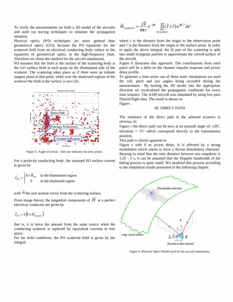
Figure 5 shows all detected rays during a final approach seenfrom the receiver antenna. Clusters indicate the direct signal, areflection zone on the fuselage and a ground reflection. The blacklines are edges of the airplanes structure, indicating e.g. the wings,engines and fuselage.

Figure 3: Channel impulse response of the final approach in a large time scale

Figure 4: Measured impulse response – short time scalePhysical Optics (PO) Simulation

To verify the measurements we built a 3D model of the aircraftsand used ray tracing techniques to simulate the propagationsituation.Physical optics (PO) techniques are more general thangeometrical optics (GO), because the PO equations for thescattered field from an electrical conducting body reduce to theequations of geometrical optics in the high-frequency limit.Therefore we chose this method for the aircraft simulations.PO assumes that the field at the surface of the scattering body isthe GO surface field at each point on the illuminated side of thescatterer. The scattering takes place as if there were an infinitetangent plane at that point, while over the shadowed regions of thescatterer the field at the surface is zero [4].

Figure 5: Angle of arrival – Dot size indicates the echo power.

For a perfectly conducting body, the assumed PO surface currentis given by

×=

region shadowed in the0

region dilluminate in theˆˆPO

TotHnJ�

with n̂ the unit normal vector from the scattering surface.

From image theory, the tangential components of H�

at a perfectelectrical conductor are given by

( )IncidentHnJ ˆˆ2PO ×=�

that is, it is twice the amount from the same source when theconducting scatterer is replaced by equivalent currents in freespace.For far field conditions, the PO scattered field is given by theintegral

∫∫ ⋅− ×≈surfaceLit

’ˆ ’)ˆ(4

dserJer

jH rrjrj

Scattered

���

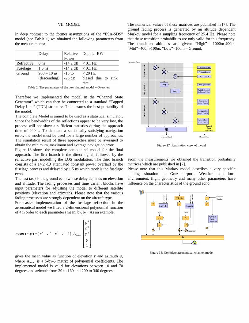
where r is the distance from the origin to the observation pointand r’ is the distance from the origin to the surface point. In orderto apply the above integral, the lit part of the scattering is splitinto small triangular patches to approximate the curved surface ofthe aircraft.Figure 6 illustrates this approach. The contributions from eachpatch will be a delta on the channel impulse response and powerdelay profile.To generate a time series out of these static simulations we usedthe roll, pitch and jaw angles being recorded during themeasurement. By turning the 3D model into the appropriatedirection we recalculated the propagation conditions for everytime instance. The A340 aircraft was simulated by using low passfiltered flight data. The result is shown inFigure .

III. DIRECT PATH

The existence of the direct path in the selected scenario isobvious. InFigure 5 the direct path can be seen at an azimuth angle of -120°,elevation = 15° which correspond directly to the transmissionposition.This path is clearly apparent inFigure 4 with 0 ns access delay. It is affected by a strongmodulation which seems to have a Rician distribution character.Bearing in mind that the time distance between two snapshots is1.25 - 5 s, it can be assumed that the Doppler bandwidth of thefading process is quite small. We modeled this process accordingto the simulation results presented in the following chapter.

Figure 6: Physical Optics Model used for the aircraft simulations.

IV. WING REFLECTION

The inventors of the ESA-SDS Model expected a strong reflectionfrom the wings (see Table 1). We had been very surprised that wewere not able to find any wing reflection in the measurement,neither Figure 4 nor Figure 5 showed a hint to this reflection type.For this reason we used the physical optics model to determinethe expected reflection power. The result of this simulation was asurprise: The power of the wing reflection was around –35 dB(see . Figure 8 (ATTAS) at around 40-50 ns and Figure 9 (A 340)at 50-80 ns). This explains why we were not able to identify thisreflection. This extremely low power level made clear that fromno relevant error contribution can result from the wing. For thisreason we decided not to model this reflection type.

Figure 7: 3D model ATTAS. Green surfaces are visible from the antenna (red dot)

V. FUSELAGE REFLECTION

Examinations of the impulse response plot (Figure 4) and AOA(Figure 5) plot shows that there is a quite strong reflection veryclose to the LOS signal at approximately 1-2 ns delay with acertain modulation on it. This is most easily seen in Figure 9,which is a detail of Figure 3.The highest likelihood for receiving reflections is locatedapproximately at an elevation of -10 degrees. This position is justbelow the receiver antenna on the fuselage. Therefore we will callthis reflection the “fuselage echo”. The power of this echo isestimated to –14.2 dB. Again, having in mind the timing grid, weassume the Doppler bandwidth of this process also to be below0.1 Hz.The existence of the fuselage reflection was proven by a POsimulation. Figure 10 is showing its result. In this scenario theA340 was illuminated from the left side and an elevation of 15

degrees. The colour indicates the power received from therespective reflection areas. There the fuselage echo can clearly beseen as an orange spot close to the antenna on top of the cockpit.

Figure 8: PO Simulation ATTAS – time series

Further trials to find another reflection were carried out. Onlooking carefully on the plots, another reflection could beassumed at approximately 2 - 4 ns. Under closer scrutiny wefigured that these estimated rays are often coming from “nowherein the sky” or from always changing directions. Therefore we arenot able to identify a reflection in this delay range. All the otherreflections shown in the figures cannot be associated to adistinguished part of the airplane. That’s why we assume thatthese “spots” are artifacts or false estimates of the ISIS algorithm.This is the same case for longer delayed reflections. In order toprove this assumption we took a closer look on the circular flightdata. Again no clear echo could be found caused by the airplanestructure. The non-existence of another strong reflection can beseen in Figure 10. Therefore we assume the fuselage echo to bethe only aircraft structure reflection. For the implementation itsbandwidth has to be determined.

Figure 9: PO Simulation Airbus A340 - time series

Since the bandwidth of the fuselage echo is extremely small theISIS algorithm is not able to estimate it. To further investigate thefuselage process, we performed the following simulation:During the flight the experimental jet ATTAS recorded itsmovements. We used the measured roll, yaw and pitch data tomodel the aircrafts orientation in the air. During the finalapproach roll, pitch and yaw angles were recorded on theATTAS. For the aircrafts fuselage a simple cylinder model wasused. For the ATTAS a mean fuselage radius of r = 1.435 m andan antenna height of 5 cm (as during the measurements) was takenfor the model. We assumed an infinite far satellite, therefore wehave parallel incoming signals for our model. Now we calculatedthe reflection points on the surface as the elevation and azimuthslightly changes during the landing. For each data point the angleof arrival was varied according to the flight data by rotating thecylinder model with its antenna. So for each time instance the

Figure 9: Measured impulse response

Figure 10: PO simulation of the A340. The colour indicates the strength of powercontribution to the impulse response (red areas contribute a lot).

From Satellite

direct

reflected

Fuselage

2870 mm

5 cm

Figure 11: Simulating the fuselage echo

reflection point on the cylinder and the excess length of thereflected ray, which is proportional to its relative phase, iscalculated by

∆⋅−=

λπ s

jtsts rec

2exp*)()(

where s∆ is the distance change and λ is the wavelength.

Figure 12: Fuselage echo spectrum

This time variant phase shift causes a parasitic phase modulation.From this process, compared to the direct path, we obtained thefollowing spectrum, as an example for 15° elevation and 75°azimuth (satellite position) in Figure 12. This spectrum shows,that there is a very strong constant (DC) component overlaid by anoisy process (fuselage process). The fuselage process can beapproximated very well by an exponential function by using non-linear regression. The result is shown as well in the examples. Thefuselage process is shown only up to a bandwidth of 2 Hz sincethe recorded ATTAS flight data was sampled at 2 Hz. Analysis of

the fuselage reflections identified in the ISIS estimated powerdelay profile indicate that this exponential spectrum has asignificant larger bandwidth.

We assumed the modulation of the direct path to be highlycorrelated with the fuselage process, because they are very closein terms of delay. So for the final model we modulated also thedirect path signal with this process.To expand our fuselage process model for different elevation andazimuth angles of the incoming rays, we repeated the simulationfor other elevations and azimuths (Fuselage Igloo Approach).All these simulations were performed for the GPS L1 frequencyof 1575.42 MHz. For the simulation the ATTAS roll, pitch andyaw data which had been recorded every 0.5 seconds wereinterpolated in order to not limit the bandwidth of the simulatedfuselage echo. A quarter of an “igloo” was simulated forelevations and azimuths between 0 and 90 degrees in 5 degreesteps. Azimuth 0 degrees points to the nose of the plane. For eachdata point of the igloo the angle of arrival was varied according tothe flight data by rotating the cylinder model with its antenna.Due to the fact that the airplanes fuselage is not a cylinder, thecylindrical model shows an accuracy limit for azimuths around 0and 180 degrees. For this the igloo was limited to elevations from10 to 70 degrees and azimuths between 20 and 90 degrees. Thefollowing figures show the simulation results for the parametersmean, b2 and b3 of the fuselage echo spectrum, where b2 and b3

are the coefficients of the exponential process:

( ) fbproc ebkdBp ⋅⋅+= 3

2

Please note that the total power of this process had been measuredto be –14.2 dB which determines the constant k = -14.2 - mean[dB] in the end. The smallest inner circle is 75 degree elevationand the largest on the outside gives the values for 5 degreeelevation. The azimuth varies from 15 to 165 and 195 to 335degrees respectively.

This simulation shows that the fuselage characteristics changevery little by increasing the fuselage radius.The mean value clearly decreases as the elevation decreases, thatis because the variation in the fuselage reflection is higher due tothe movement of the plane, which is mainly a rotation around theroll axis. We can also see that the mean value is smaller if thesatellite is in front or in the rear of the plane.The scaling factor for the exponential part of the fuselagespectrum b2 does not vary much. It is a little bit higher if thesatellite is at the side of the airplane. More significant is thebehaviour of the exponent b3. This parameter is highest for lowelevations and azimuth directions front and rear. That means, forthis situation the bandwidth is larger and therefore less criticalcompared to a satellite at high elevations at the side of the plane.

When we compare these results to the simulation of the Airbuswith its larger fuselage radius, we can e.g. see that the mean valueis even smaller at low elevations. There is more variation andtherefore a larger bandwidth. The parameters are very similar tothe results of the ATTAS simulation. Over all, the fuselagereflection seems to have a slightly larger bandwidth for theAirbus. The values of the matrices are attached in the appendix ofthis paper.

VI. GROUND REFLECTION

In Figure 13 the ground reflection can be seen clearly prior totouch down in a larger time scale to display the ground reflection.It can explicitly be seen that the ground reflection has a quite lowpower. The dynamic range can be estimated to -15 to -25 dB.The delay is dependent on the altitude and is varying between 900and 10 ns.

Figure 13: Flight 2_7 in a large time scale

For the ground reflection the Doppler spread is large enough forISIS to estimate. We are now going to determine the spectrum ofthe ground reflection.The desired descending speed was around 5 m/s, which is relatedto the strong components at 25 Hz. In the last phase of theapproach, shortly before touch down, the descending speeddecreases and, possibly from the runway, strong reflections can beseen between 10 and 20 Hz offset.Figure 14 gives the ISIS Doppler estimation as function of theactual sink rate during the whole landing approach. The green lineindicates the linear regression of the data. It is obvious that theDoppler shift is related to the sink rate of the plane. Due to thatthe Doppler shift will be zero for a horizontally flying airplane.For this reason we force a zero crossing interpolation (red line) togive us the momentarily Doppler offset. A Doppler offset ofapproximately 6 Hz/(m/s) = 6 wavelengths/m ≈ 1/λ = 6,3 wave-lengths/m. can be estimated. This finally proofs that the constantDoppler shift had been caused by the vertical speed.Removing the Doppler offset from this data we plot the remaining

power weighted ground reflection Doppler distribution of theapproaching plane. Figure 15 indicates that the bandwidth of theground Doppler process is < 10 Hz.Assuming a Gauss distributed ground reflection amplitude withzero mean, we can model the spectrum by

)*(log*202

2

210)(

σ

f

ekP dBGr

−=

where the deviation σ�� ���� ��� �� �� ����� � �� ��� ��� ���flight 2 measurement 7 (σ����������� �������������� ���������(σ���������������������������� �����������������������Figure 15for flight 3 measurement 6.Please note that the Doppler bandwidth of 420 Hz in the oldmodel [1] is significantly too high. For the implementation of theground reflection model the parameter σ can be linearly scaled tothe L1 frequency of 1575.42 MHz.

Figure 14: Doppler offset versus sink rate

This concludes the definition of the Doppler process for theground reflection.Figure 16 shows the occurrence of the ground echo. It is quiteobvious that the ground Echo is modulated by the reflectingterrain structure. To extract this process we divide the finalapproach into 3 different zones of altitude (high, mid and lowaltitude). In each zone the ground reflection is characterized by aMarkov state model [6]. Furthermore we divided the occurringpower levels in four power levels (-15dB, -19dB, -23dB, <-25dB).Now we can obtain the Markov parameters from the quantisedmeasurement data. The transition matrix P where Px,y is theprobability of changing from state x to state y is determined foreach altitude region independently.

Hzf

f

meas

LL 0.31

1 == σσ

Figure 15: Doppler spectrum of ground reflection after vertical speed correction

Figure 16: Altitude dependent ground echo occurrence

The delay of the ground reflection as function of the elevation canbe easily calculated assuming a flat environment around theairport by

0

)sin()(2)(

C

thtground

ετ ⋅⋅=

where h(t) is the current altitude and ε is the elevation angle.

VII. MODEL

In deep contrast to the former assumptions of the “ESA-SDS”model (see Table 1) we obtained the following parameters fromthe measurements:

Delay RelativePower

Doppler BW

Refractive 0 ns -14.2 dB < 0.1 HzFuselage 1.5 ns -14.2 dB < 0.1 HzGround 900 – 10 ns

(descending)-15 to-25 dB

< 20 Hzbiased due to sinkrate

Table 2: The parameters of the new channel model – Overview

Therefore we implemented the model in the “Channel StateGenerator” which can then be connected to a standard “TappedDelay Line” (TDL) structure. This ensures the best portability ofthe model.The complete Model is aimed to be used as a statistical simulator.Since the bandwidths of the reflections appear to be very low, theprocess will not show a sufficient statistics during the approachtime of 200 s. To simulate a statistically satisfying navigationerror, the model must be used for a large number of approaches.The simulation result of these approaches must be averaged toobtain the minimum, maximum and average navigation error.Figure 18 shows the complete aeronautical model for the finalapproach. The first branch is the direct signal, followed by therefractive part modelling the LOS modulation. The third branchconsists of a 14.2 dB attenuated constant power overlaid by thefuselage process and delayed by 1.5 ns which models the fuselageecho.The last tasp is the ground echo whose delay depends on elevationand altitude. The fading processes and time variant blocks haveinput parameters for adjusting the model to different satellitepositions (elevation and azimuth). Please note that the variousfading processes are strongly dependent on the aircraft type.For easier implementation of the fuselage reflection in theaeronautical model we fitted a 2-dimensional polynomial functionof 4th order to each parameter (mean, b2, b3). As an example,

⋅⋅=

1

]1[),( 2

3

4

234

ϕϕϕϕ

εεεεϕε meanAmean

gives the mean value as function of elevation ε and azimuth ϕ,where Amean is a 5-by-5 matrix of polynomial coefficients. Theimplemented model is valid for elevations between 10 and 70degrees and azimuth from 20 to 160 and 200 to 340 degrees.

The numerical values of these matrices are published in [7]. Theground fading process is generated by an altitude dependentMarkov model for a sampling frequency of 25.4 Hz. Please notethat these transition probabilities are only valid for this frequency.The transition altitudes are given: “High”= 1000m-400m,“Mid”=400m-100m, “Low”=100m – Ground.

Figure 17: Realisation view of model

From the measurements we obtained the transition probabilitymatrices which are published in [7].Please note that this Markov model describes a very specificlanding situation at Graz airport. Weather conditions,environment, flight geometry and many other parameters haveinfluence on the characteristics of the ground echo.

Figure 18: Complete aeronautical channel model

VIII. CONCLUSION

We presented a high resolution aeronautical multipath modelcomprising detailed investigations on reflections on aircraftstructures and ground reflections during final approach.Measurements and simulations show a strong reflection at thefuselage close to the antenna as the main contribution to thepositioning error. We may safely assume that wing reflections arenegligible and that echo bandwidths were assumed far too large inthe past. And we were able to approve measurement results andsimulation methods.

„Ground Fading Generator“

State1

State4State3

State2

Ground Path Fading Process

WGN

State1

State4State3

State2

State1

State4State3

State2

Doppler Spectrum

Filter

0

Altitude

Figure 19: Realisation of the ground fading generator module

IX. MODEL DOWNLOAD

The implemented model is available for download. We refer tothe following web sites:

http://www.dlr.de/kn/kn-s/steingasshttp://www.dlr.de/kn/kn-s/lehner

X. AKNOWLEDGEMENTS

The work presented in this paper was carried out under aEuropean Space Agency, ESA, contract entitled "Navigationsignal measurement campaign for critical environments", byJOANNEUM RESEARCH (Austria) with subcontracts to DLR(Germany) and the University of Vigo (Spain).

REFERENCES

[1] R. Schweikert, T. Woerz. Signal design and transmissionperformance study for GNSS-2. Final Report, EuropeanSpace Agency, 1998.

[2] Andreas Lehner, Alexander Steingaß, "The Influence ofMultipath to Navigation Receivers", Global NavigationSatellite Systems Conference (GNSS2003), Graz, Austria

[3] Xuefeng Yin, Bernard H. Fleury, Patrik Jourdan andAndreas Stucki, “Doppler Frequency Estimation for ChannelSounding Using Switched Multiple Transmit and ReceiveAntennas”, GLOBECOM 2003, San Francisco, USA.

[4] W. L. Stutzman and G. A. Thiele Antenna Theory anddesign John Wiley, 1981.

[5] B.W. Parkinson, J.J. Spilker “Global Positioning SystemTheory and Applications I + II”, Volume 164 of Progress inAstronautics and Aeronautics. American Institute ofAeronautics and Astronautics Inc. Washington 1996.

[6] Athanasios Papoulis, “Probability, Random Variables andStochastic Processes” Mc Graw-Hill Book Company, NewYork, 1965

[7] Alexander Steingass, Andreas Lehner, Fernando Pérez-Fontán, Erwin Kubista, Maria Jesús Martín, and BertramArbesser-Rastburg “The High Resolution AeronautiocalMultipath Navigation Channel” ION-NTM 2004, San Diego,USA.