POUR L'OBTENTION DU GRADE DE DOCTEUR ÈS SCIENCES

acceptée sur proposition du jury:

Prof. E. Sanchez, président du juryProf. A. Ijspeert, Prof. G. Tempesti, directeurs de thèse

Dr S. Bocchio, rapporteure Prof. G. de Micheli, rapporteur

Dr G. Sassatelli, rapporteur

A Hardware-Software Codesign Framework for Cellular Computing

THÈSE NO 4354 (2009)

ÉCOLE POLYTECHNIQUE FÉDÉRALE DE LAUSANNE

PRÉSENTÉE LE 5 jUIN 2009

À LA FACULTÉ INFORMATIQUE ET COMMUNICATIONS

GROUPE IjSPEERT

PROGRAMME DOCTORAL EN INFORMATIQUE, COMMUNICATIONS ET INFORMATION

Suisse2009

PAR

Pierre-André MUDRY

A ceux qui sont partiset à ceux qui restent.

Résumé

LA COURSE à la performance commencée il y a plus de trente ans dans l’industrie des processeursvoit se profiler à l’horizon d’un futur désormais proche des limites physiques qui seront difficiles à

franchir. Pour maintenir le rythme de croissance de la puissance de calcul des processeurs, l’utilisationde plusieurs unités de calcul en parallèle est désormais courante. Toutefois, cette augmentation duparallélisme n’est pas sans poser son lot de problèmes liés à la concurrence ou encore au partage desressources. De plus, peu de programmeurs possèdent aujourd’hui une connaissance suffisante de laproblématique de la programmation parallèle pour faire face à l’essor de tels systèmes.

Toutefois, le recours au parallélisme dans cette quête de performance n’exclut pas d’autres pistesde recherche telles que de nouvelles méthodes de fabrication, issues par exemple des nanotechnologies.Celles-ci imposeront probablement le renouvellement des méthodologies de conception des processeursafin de pouvoir faire face à des contraintes telles qu’un nombre accru d’erreurs matérielles ou encore laprogrammation de systèmes contenant plusieurs centaines de processeurs.

Une source d’inspiration possible pour répondre à de telles problématiques se trouve dans labiologie. En effet, les êtres vivants possèdent des caractéristiques intéressantes telles que la résistanceaux dommages, certains organismes tels que les salamandres pouvant se régénérer en partie, ouencore une organisation dynamique, des cellules étant perpétuellement remplacées par de nouvelles.Dans cette optique, un certain nombre de travaux ont mis en évidence l’intérêt d’imiter partiellementcertaines caractéristiques de ces organismes afin de les utiliser dans du matériel informatique. Ainsi,il a été possible de réaliser des systèmes relativement simples inspirés de ces mécanismes, commeune horloge auto-réparante. Toutefois, l’application de ces méthodologies pour des problèmes pluscomplexes reste très délicate en raison de la difficulté à utiliser la polyvalence proposée par ces systèmesmatériels, inhérente à une implémentation complètement matérielle qui, par nature, est complexe àprogrammer.

Dans le cadre de cette thèse, nous nous proposons d’étudier cette problématique en plaçant toutd’abord au cœur de notre approche un processeur totalement flexible, possédant d’une part descaractéristiques permettant d’appliquer des mécanismes issus de la bio-inspiration et, d’autre part,étant à même d’assumer les tâches de calcul que l’on attend généralement d’un processeur. Nousverrons ainsi qu’il est possible d’obtenir un tel processeur et que l’on peut, par exemple, le faire évoluerafin de le spécialiser pour différentes applications.

Dans un deuxième temps, nous nous proposons d’analyser comment la mise en parallèle d’ungrand nombre de ces processeurs sur une plateforme matérielle idoine permet d’explorer différentsaspects de la bio-inspiration dans des situations réelles. Nous mettrons ainsi en lumière que le principedes architectures cellulaires permet, à l’aide de différentes abstractions logicielles, d’utiliser la puissancedes processeurs tout en restant flexible. Par le biais d’une interface graphique facile d’emploi, nousillustrerons comment il est possible de simplifier la programmation de tels systèmes grâce à différentsoutils logiciels. Finalement, nous appliquerons notre jeu d’outils logiciels et matériels afin de montrer,sur des exemples concrets typiques des applications embarquées, comment l’auto-organisation et laréplication peuvent apporter certaines réponses au problème de la performance.

Mots-clés: processeur TTA, Move, matériel électronique bio-inspiré, FPGA, algorithmes d’évolution,réplication, MPSoC, routage, SSSP.

v

Abstract

UNTIL RECENTLY, the ever-increasing demand of computing power has been met on one hand byincreasing the operating frequency of processors and on the other hand by designing architectures

capable of exploiting parallelism at the instruction level through hardware mechanisms such as super-scalar execution. However, both these approaches seem to have reached a plateau, mainly due toissues related to design complexity and cost-effectiveness.

To face the stabilization of performance of single-threaded processors, the current trend in processordesign seems to favor a switch to coarser-grain parallelization, typically at the thread level. In otherwords, high computational power is achieved not only by a single, very fast and very complexprocessor, but through the parallel operation of several processors, each executing a different thread.

Extrapolating this trend to take into account the vast amount of on-chip hardware resources that willbe available in the next few decades (either through further shrinkage of silicon fabrication processesor by the introduction of molecular-scale devices), together with the predicted features of such devices(e.g., the impossibility of global synchronization or higher failure rates), it seems reasonable to foretellthat current design techniques will not be able to cope with the requirements of next-generationelectronic devices and that novel design tools and programming methods will have to be devised.

A tempting source of inspiration to solve the problems implied by a massively parallel organizationand inherently error-prone substrates is biology. In fact, living beings possess characteristics, such asrobustness to damage and self-organization, which were shown in previous research as interesting tobe implemented in hardware. For instance, it was possible to realize relatively simple systems, such asa self-repairing watch.

Overall, these bio-inspired approaches seem very promising but their interest for a wider audienceis problematic because their heavily hardware-oriented designs lack some of the flexibility achievablewith a general purpose processor.

In the context of this thesis, we will introduce a processor-grade processing element at the heartof a bio-inspired hardware system. This processor, based on a single-instruction, features some keyproperties that allow it to maintain the versatility required by the implementation of bio-inspiredmechanisms and to realize general computation. We will also demonstrate that the flexibility of such aprocessor enables it to be evolved so it can be tailored to different types of applications.

In the second half of this thesis, we will analyze how the implementation of a large number of theseprocessors can be used on a hardware platform to explore various bio-inspired mechanisms. Basedon an extensible platform of many FPGAs, configured as a networked structure of processors, thehardware part of this computing framework is backed by an open library of software components thatprovides primitives for efficient inter-processor communication and distributed computation. We willshow that this dual software–hardware approach allows a very quick exploration of different waysto solve computational problems using bio-inspired techniques. In addition, we also show that theflexibility of our approach allows it to exploit replication as a solution to issues that concern standardembedded applications.

Key words: TTA processor, Move, bio-inspired hardware, FPGA, evolutionary algorithms, MPSoC, routing,replication, SSSP.

vii

Remerciements

RÉALISER UNE thèse est un exercice de longue haleine dont il est difficile de comprendre les tenantset les aboutissants sans l’avoir vécu personnellement. Qui plus est, la thèse est un exercice qui

s’effectue majoritairement en solitaire. Toutefois, même si l’activité de la thèse elle-même ne sauraitse partager, l’environnement dans lequel celle-ci est réalisée joue un rôle primordial et qui constituela raison d’être profonde de cette page de remerciements. En effet, à quoi donc auraient ressembléces quatre ans sans votre support à vous, amis, connaissances et collègues qui avez rendu possible cetravail à divers niveaux ? À cette question, je ne peux répondre que par le témoignage de toute magratitude.

Du point de vue académique tout d’abord, celle-ci va aux membres de mon jury de thèse, à savoirGiovanni de Micheli, Gilles Sassatelli ainsi que Sara Bocchio, pour avoir amené leur expertise et leurscommentaires qui ont permis d’améliorer la version finale de ce document ainsi qu’au président dujury, Eduardo Sanchez. Merci à Gianluca Tempesti de m’avoir trouvé ce poste en me laissant une libertétotale et au Fonds national suisse de la recherche scientifique de l’avoir financé. Merci également àAuke Ijspeert de m’avoir accueilli dans son laboratoire en cours de route tout en étant une sourceintarissable et efficace de bons conseils. Finalement, je tiens également à remercier Daniel Mange poursa sympathie et pour avoir pris du temps pour que ma thèse se termine en douceur.

Au niveau de mes collègues de travail, un énorme merci va à notre “bureau du bonheur”, lieumystique de découverte musicale et d’expérience de vie à part entière. Plus précisément, merci à Sarahqui a eu la gentillesse, peut-être bien malgré elle, d’écouter mes états d’âme, doutes et autres coupsde gueule pendant une majeure partie de ma thèse. Nos multiples cafés ont constitué pour moi unvéritable bol d’air frais et je t’en remercie. Merci également à Ludovic, pour nos festives escapades etpour avoir partagé avec moi ses expériences de fin de thèse. Je dois également tirer ma casquette àAlessandro, capable de résoudre absolument tous les problèmes informatiques, souvent même avantqu’ils apparaissent. Merci pour ton aide et ta gentillesse !

J’en profite également pour remercier les étudiants qui m’ont amené par leur travail de l’aide surdifférents points de cette recherche. Plus particulièrement, un grand merci à Guillaume pour le chapitresur l’évolution ainsi que pour le temps que nous avons passé ensemble à travailler et que j’ai beaucoupapprécié. Merci également à Julien pour son travail acharné sur CAFCA et SSSP et à Michel pour lecompilateur.

Bien entendu, avant d’arriver à la thèse, mon parcours a inclus plusieurs années d’étude que j’aieu le plaisir de traverser avec des gens qui méritent la plus grande estime. Un énorme merci donc àDavid, programmeur emeritus aux multiples traits de génie dont la dextérité au clavier n’a d’égaleque la rapidité de programmation et avec qui j’ai eu l’immense honneur de travailler depuis noslaborieux débuts au Poly. Je n’ai jamais autant appris qu’avec toi et ton niveau surhumain m’a forcéà me dépasser constamment, ne serait-ce que pour pouvoir te suivre, enfin sauf en ce qui concerneles flancs d’horloge bien sûr ! Merci aussi à Leto, dont le travail a toujours réussi à conserver cetteaura de magie qui fait rêver. Finalement, merci à Bertrand pour nos toujours sympathiques repas etdiscussions qui couvraient tant les jeux vidéo que les mathématiques les plus complexes auxquelles jefaisais péniblement semblant de comprendre quelque chose.

Le travail étant une chose, il y a une vie en dehors de celui-ci et je n’en serais pas là aujourd’huisans des gens très importants pour moi. Merci donc à Igor, pilote chevronné de presque tous lesmoyens de transport existants, blagueur hors pair qui a même réussi, de manière étonnante et ceci àplusieurs reprises, à me prendre dans son avion. Faire l’école buissonière et manger de la pizza avec

ix

toi comptent clairement parmis mes activités préférées ! Merci aussi, sans aucun ordre particulier, àAntonin pour toutes nos activités campagnardes, à Maître Charvet pour ses discussions avec Rachel, àTorrent pour sa vision du monde, à l’officieux Club de Chibre et à ses membres pour avoir occupé biendes dimanches après-midi, à A.S. pour m’avoir montré quelques arbres dans la forêt et à Depeche Modepour leur musique.

Merci encore à Jacqueline, Pascal et Laurence pour leur accueil ainsi que pour leur gentillessedepuis plus de dix ans maintenant.

Un grand merci à ma famille, dont le dévouement m’a offert l’opportunité de faire mes études etsans qui rien n’aurait été possible.

Le dernier mot sera finalement pour Rachel, incroyable amie qui m’a accompagné pendant unebelle partie de mon chemin et sans qui la vie serait définitivement bien moins drôle. Merci de toutcœur, je n’y serais pas arrivé sans toi !

Contents

1 Introduction 11.1 Motivations and background . . . . . . . . . . . . . . . . . . . . . . . . . . . . . . . . . . 1

1.1.1 The bio-inspired approach . . . . . . . . . . . . . . . . . . . . . . . . . . . . . . . 21.1.2 Cellular architectures . . . . . . . . . . . . . . . . . . . . . . . . . . . . . . . . . . 2

1.2 Objectives . . . . . . . . . . . . . . . . . . . . . . . . . . . . . . . . . . . . . . . . . . . . . 31.3 Thesis plan and contributions . . . . . . . . . . . . . . . . . . . . . . . . . . . . . . . . . . 4

1.3.1 Part 1: A highly customizable processing element . . . . . . . . . . . . . . . . . . 41.3.2 Part 2: Networks of processing elements . . . . . . . . . . . . . . . . . . . . . . . 4

I A highly customizable processing element 9

2 Towards transport triggered architectures 112.1 Introduction . . . . . . . . . . . . . . . . . . . . . . . . . . . . . . . . . . . . . . . . . . . . 11

2.1.1 Preliminary note . . . . . . . . . . . . . . . . . . . . . . . . . . . . . . . . . . . . . 112.2 On processor architectures . . . . . . . . . . . . . . . . . . . . . . . . . . . . . . . . . . . 122.3 RISC architectures . . . . . . . . . . . . . . . . . . . . . . . . . . . . . . . . . . . . . . . . 12

2.3.1 Improving performance . . . . . . . . . . . . . . . . . . . . . . . . . . . . . . . . . 132.4 VLIW architectures . . . . . . . . . . . . . . . . . . . . . . . . . . . . . . . . . . . . . . . . 132.5 Transport triggered architectures . . . . . . . . . . . . . . . . . . . . . . . . . . . . . . . . 15

2.5.1 Beyond VLIW . . . . . . . . . . . . . . . . . . . . . . . . . . . . . . . . . . . . . . 152.5.2 Introducing the Move–TTA approach . . . . . . . . . . . . . . . . . . . . . . . . . 162.5.3 From implicit to explicit specification . . . . . . . . . . . . . . . . . . . . . . . . . 162.5.4 Exposing various levels of connectivity . . . . . . . . . . . . . . . . . . . . . . . . 17

2.6 TTA advantages and disadvantages . . . . . . . . . . . . . . . . . . . . . . . . . . . . . . 182.6.1 Architecture strengths . . . . . . . . . . . . . . . . . . . . . . . . . . . . . . . . . . 182.6.2 Architecture weaknesses . . . . . . . . . . . . . . . . . . . . . . . . . . . . . . . . 20

2.7 A flexible operation-set . . . . . . . . . . . . . . . . . . . . . . . . . . . . . . . . . . . . . 212.8 TTA and soft-cores . . . . . . . . . . . . . . . . . . . . . . . . . . . . . . . . . . . . . . . . 212.9 Conclusion . . . . . . . . . . . . . . . . . . . . . . . . . . . . . . . . . . . . . . . . . . . . 22

3 The ULYSSE processor 273.1 Internal structure overview . . . . . . . . . . . . . . . . . . . . . . . . . . . . . . . . . . . 273.2 Simplified operation . . . . . . . . . . . . . . . . . . . . . . . . . . . . . . . . . . . . . . . 28

3.2.1 Operation example . . . . . . . . . . . . . . . . . . . . . . . . . . . . . . . . . . . 283.2.2 Triggering schemes . . . . . . . . . . . . . . . . . . . . . . . . . . . . . . . . . . . 29

3.3 Different CPU versions . . . . . . . . . . . . . . . . . . . . . . . . . . . . . . . . . . . . . 303.4 Interconnection network . . . . . . . . . . . . . . . . . . . . . . . . . . . . . . . . . . . . . 30

3.4.1 Single slot instructions . . . . . . . . . . . . . . . . . . . . . . . . . . . . . . . . . 313.4.2 Instruction format and inner addressing . . . . . . . . . . . . . . . . . . . . . . . 32

3.5 A common bus interface . . . . . . . . . . . . . . . . . . . . . . . . . . . . . . . . . . . . . 333.6 The fetch unit . . . . . . . . . . . . . . . . . . . . . . . . . . . . . . . . . . . . . . . . . . . 34

3.6.1 Pipelining functional units . . . . . . . . . . . . . . . . . . . . . . . . . . . . . . . 363.7 Memory interface unit . . . . . . . . . . . . . . . . . . . . . . . . . . . . . . . . . . . . . . 38

xi

CONTENTS

3.7.1 Embedded memory controller . . . . . . . . . . . . . . . . . . . . . . . . . . . . . 383.7.2 Asynchronous SRAM FU and controller . . . . . . . . . . . . . . . . . . . . . . . 39

3.8 ULYSSE functional units . . . . . . . . . . . . . . . . . . . . . . . . . . . . . . . . . . . . . 423.8.1 Concatenation unit . . . . . . . . . . . . . . . . . . . . . . . . . . . . . . . . . . . 443.8.2 Conditional instructions (condition unit) . . . . . . . . . . . . . . . . . . . . . . . 443.8.3 Arithmetic and logic functional (ALU) unit . . . . . . . . . . . . . . . . . . . . . 44

3.9 Hardware performance evaluation . . . . . . . . . . . . . . . . . . . . . . . . . . . . . . . 453.9.1 Ulysse’s FU size and speed . . . . . . . . . . . . . . . . . . . . . . . . . . . . . . . 45

3.10 Possible further developments . . . . . . . . . . . . . . . . . . . . . . . . . . . . . . . . . 453.10.1 Permanent connections and meta-operators . . . . . . . . . . . . . . . . . . . . . 46

3.11 Conclusion . . . . . . . . . . . . . . . . . . . . . . . . . . . . . . . . . . . . . . . . . . . . 48

4 Development tools 514.1 The assembler . . . . . . . . . . . . . . . . . . . . . . . . . . . . . . . . . . . . . . . . . . . 51

4.1.1 Assembly process . . . . . . . . . . . . . . . . . . . . . . . . . . . . . . . . . . . . 514.1.2 Memory map definition with file inclusion . . . . . . . . . . . . . . . . . . . . . . 534.1.3 Definition of new operators . . . . . . . . . . . . . . . . . . . . . . . . . . . . . . 544.1.4 Macros and their influence on the definition of a meta-language . . . . . . . . . 544.1.5 Code and data segments . . . . . . . . . . . . . . . . . . . . . . . . . . . . . . . . 554.1.6 Arithmetic expressions . . . . . . . . . . . . . . . . . . . . . . . . . . . . . . . . . 564.1.7 Immediate values and far jumps . . . . . . . . . . . . . . . . . . . . . . . . . . . . 564.1.8 Miscellaneous items . . . . . . . . . . . . . . . . . . . . . . . . . . . . . . . . . . . 584.1.9 JavaCC . . . . . . . . . . . . . . . . . . . . . . . . . . . . . . . . . . . . . . . . . . 584.1.10 Language grammar . . . . . . . . . . . . . . . . . . . . . . . . . . . . . . . . . . . 59

4.2 GCC back-end . . . . . . . . . . . . . . . . . . . . . . . . . . . . . . . . . . . . . . . . . . 594.2.1 Why GCC ? . . . . . . . . . . . . . . . . . . . . . . . . . . . . . . . . . . . . . . . . 594.2.2 The GNU C Compiler – GCC . . . . . . . . . . . . . . . . . . . . . . . . . . . . . . 604.2.3 GCC components . . . . . . . . . . . . . . . . . . . . . . . . . . . . . . . . . . . . 604.2.4 The compilation process . . . . . . . . . . . . . . . . . . . . . . . . . . . . . . . . 60

4.3 Handling function calls . . . . . . . . . . . . . . . . . . . . . . . . . . . . . . . . . . . . . 614.3.1 Saving state . . . . . . . . . . . . . . . . . . . . . . . . . . . . . . . . . . . . . . . . 624.3.2 GCC optimizations . . . . . . . . . . . . . . . . . . . . . . . . . . . . . . . . . . . 624.3.3 ULYSSE peculiarities for GCC . . . . . . . . . . . . . . . . . . . . . . . . . . . . . 634.3.4 Compiler optimizations specific to TTA . . . . . . . . . . . . . . . . . . . . . . . . 64

4.4 Conclusion . . . . . . . . . . . . . . . . . . . . . . . . . . . . . . . . . . . . . . . . . . . . 66

5 Testing and performance evaluation 695.1 Testing methodology . . . . . . . . . . . . . . . . . . . . . . . . . . . . . . . . . . . . . . . 69

5.1.1 Definitions . . . . . . . . . . . . . . . . . . . . . . . . . . . . . . . . . . . . . . . . 695.2 Testing with asserted simulation . . . . . . . . . . . . . . . . . . . . . . . . . . . . . . . . 715.3 In-circuit debugging . . . . . . . . . . . . . . . . . . . . . . . . . . . . . . . . . . . . . . . 735.4 Hierarchical testing of processor components . . . . . . . . . . . . . . . . . . . . . . . . 745.5 Processor validation, performance and results . . . . . . . . . . . . . . . . . . . . . . . . 76

5.5.1 Description of the benchmark suite . . . . . . . . . . . . . . . . . . . . . . . . . . 775.6 Code size comparisons . . . . . . . . . . . . . . . . . . . . . . . . . . . . . . . . . . . . . 805.7 Comparing simulation and execution times . . . . . . . . . . . . . . . . . . . . . . . . . 815.8 Conclusion . . . . . . . . . . . . . . . . . . . . . . . . . . . . . . . . . . . . . . . . . . . . 81

6 Processor evolution 856.1 Introduction and motivations . . . . . . . . . . . . . . . . . . . . . . . . . . . . . . . . . . 856.2 Partitioning with TTA . . . . . . . . . . . . . . . . . . . . . . . . . . . . . . . . . . . . . . 866.3 A basic genetic algorithm for partitioning . . . . . . . . . . . . . . . . . . . . . . . . . . . 86

6.3.1 Programming language and profiling . . . . . . . . . . . . . . . . . . . . . . . . . 866.3.2 Genome encoding . . . . . . . . . . . . . . . . . . . . . . . . . . . . . . . . . . . . 87

xii

CONTENTS

6.3.3 Genetic operators . . . . . . . . . . . . . . . . . . . . . . . . . . . . . . . . . . . . 886.3.4 Fitness evaluation . . . . . . . . . . . . . . . . . . . . . . . . . . . . . . . . . . . . 89

6.4 An hybrid genetic algorithm . . . . . . . . . . . . . . . . . . . . . . . . . . . . . . . . . . 926.4.1 Leveling the representation via hierarchical clustering . . . . . . . . . . . . . . . 926.4.2 Pattern-matching optimization . . . . . . . . . . . . . . . . . . . . . . . . . . . . . 936.4.3 Non-optimal block pruning . . . . . . . . . . . . . . . . . . . . . . . . . . . . . . 94

6.5 User interface . . . . . . . . . . . . . . . . . . . . . . . . . . . . . . . . . . . . . . . . . . . 946.6 Operation example . . . . . . . . . . . . . . . . . . . . . . . . . . . . . . . . . . . . . . . . 956.7 Experimental results . . . . . . . . . . . . . . . . . . . . . . . . . . . . . . . . . . . . . . . 976.8 Conclusion and future work . . . . . . . . . . . . . . . . . . . . . . . . . . . . . . . . . . 99

II Networks of processing elements 103

7 The CONFETTI platform 1057.1 Introduction and motivations . . . . . . . . . . . . . . . . . . . . . . . . . . . . . . . . . . 1057.2 Background . . . . . . . . . . . . . . . . . . . . . . . . . . . . . . . . . . . . . . . . . . . . 106

7.2.1 The BioWall . . . . . . . . . . . . . . . . . . . . . . . . . . . . . . . . . . . . . . . . 1067.3 The CONFETTI experimentation platform . . . . . . . . . . . . . . . . . . . . . . . . . . . 107

7.3.1 Overview – A hierarchical construction . . . . . . . . . . . . . . . . . . . . . . . . 1087.3.2 The cell board . . . . . . . . . . . . . . . . . . . . . . . . . . . . . . . . . . . . . . 1097.3.3 The routing board . . . . . . . . . . . . . . . . . . . . . . . . . . . . . . . . . . . . 1107.3.4 The power supply board . . . . . . . . . . . . . . . . . . . . . . . . . . . . . . . . 1117.3.5 The display board . . . . . . . . . . . . . . . . . . . . . . . . . . . . . . . . . . . . 112

7.4 The CONFETTI system . . . . . . . . . . . . . . . . . . . . . . . . . . . . . . . . . . . . . . 1137.4.1 Power consumption considerations . . . . . . . . . . . . . . . . . . . . . . . . . . 1137.4.2 Thermal management . . . . . . . . . . . . . . . . . . . . . . . . . . . . . . . . . . 1137.4.3 Integrated test and monitoring . . . . . . . . . . . . . . . . . . . . . . . . . . . . . 114

7.5 Conclusion and future work . . . . . . . . . . . . . . . . . . . . . . . . . . . . . . . . . . 115

8 CONFETTI communication and software support 1198.1 Introduction and motivations . . . . . . . . . . . . . . . . . . . . . . . . . . . . . . . . . . 1198.2 High-speed communication links . . . . . . . . . . . . . . . . . . . . . . . . . . . . . . . 1208.3 Routing data in hardware . . . . . . . . . . . . . . . . . . . . . . . . . . . . . . . . . . . . 121

8.3.1 Basic features of NoC communication . . . . . . . . . . . . . . . . . . . . . . . . . 1228.3.2 Brief existing NoC overview . . . . . . . . . . . . . . . . . . . . . . . . . . . . . . 1238.3.3 The HERMES NoC . . . . . . . . . . . . . . . . . . . . . . . . . . . . . . . . . . . . 1238.3.4 MERCURY’s additions to HERMES . . . . . . . . . . . . . . . . . . . . . . . . . . . 125

8.4 Two additional functional units for ULYSSE . . . . . . . . . . . . . . . . . . . . . . . . . . 1258.4.1 The MERCURY FU . . . . . . . . . . . . . . . . . . . . . . . . . . . . . . . . . . . . 1258.4.2 Display and interface FU . . . . . . . . . . . . . . . . . . . . . . . . . . . . . . . . 128

8.5 A software API for routing . . . . . . . . . . . . . . . . . . . . . . . . . . . . . . . . . . . 1288.5.1 Related work . . . . . . . . . . . . . . . . . . . . . . . . . . . . . . . . . . . . . . . 1288.5.2 The CONFITURE communication infrastructure . . . . . . . . . . . . . . . . . . . 129

8.6 A sample application: simulating synchronicity with CAFCA . . . . . . . . . . . . . . . 1328.7 Conclusion and future work . . . . . . . . . . . . . . . . . . . . . . . . . . . . . . . . . . 133

9 A software environment for cellular computing 1419.1 Introduction and motivations . . . . . . . . . . . . . . . . . . . . . . . . . . . . . . . . . . 1429.2 Graphical programming languages . . . . . . . . . . . . . . . . . . . . . . . . . . . . . . 1429.3 A programming model . . . . . . . . . . . . . . . . . . . . . . . . . . . . . . . . . . . . . 143

9.3.1 Directed acyclic graphs programs . . . . . . . . . . . . . . . . . . . . . . . . . . . 1439.3.2 Dataflow / stream programming . . . . . . . . . . . . . . . . . . . . . . . . . . . 144

9.4 Software framework overview . . . . . . . . . . . . . . . . . . . . . . . . . . . . . . . . . 1459.5 Task programming tools . . . . . . . . . . . . . . . . . . . . . . . . . . . . . . . . . . . . . 147

xiii

CONTENTS

9.5.1 Task programming using templates . . . . . . . . . . . . . . . . . . . . . . . . . . 1479.5.2 Task compilation . . . . . . . . . . . . . . . . . . . . . . . . . . . . . . . . . . . . . 1489.5.3 Task simulation . . . . . . . . . . . . . . . . . . . . . . . . . . . . . . . . . . . . . 1499.5.4 Task profiling . . . . . . . . . . . . . . . . . . . . . . . . . . . . . . . . . . . . . . . 1499.5.5 Task library . . . . . . . . . . . . . . . . . . . . . . . . . . . . . . . . . . . . . . . . 150

9.6 Task graph programming . . . . . . . . . . . . . . . . . . . . . . . . . . . . . . . . . . . . 1519.6.1 The graph editor . . . . . . . . . . . . . . . . . . . . . . . . . . . . . . . . . . . . . 1519.6.2 Timing simulation . . . . . . . . . . . . . . . . . . . . . . . . . . . . . . . . . . . . 1519.6.3 Parallel simulation . . . . . . . . . . . . . . . . . . . . . . . . . . . . . . . . . . . . 1549.6.4 Tasks placement . . . . . . . . . . . . . . . . . . . . . . . . . . . . . . . . . . . . . 1559.6.5 Graph compilation . . . . . . . . . . . . . . . . . . . . . . . . . . . . . . . . . . . . 1559.6.6 Graph execution . . . . . . . . . . . . . . . . . . . . . . . . . . . . . . . . . . . . . 157

9.7 Conclusion . . . . . . . . . . . . . . . . . . . . . . . . . . . . . . . . . . . . . . . . . . . . 157

10 Self-scaling stream processing 16310.1 Introduction and motivations . . . . . . . . . . . . . . . . . . . . . . . . . . . . . . . . . . 16310.2 Self-scaling stream processing . . . . . . . . . . . . . . . . . . . . . . . . . . . . . . . . . 164

10.2.1 Task migration . . . . . . . . . . . . . . . . . . . . . . . . . . . . . . . . . . . . . . 16410.2.2 Task duplication . . . . . . . . . . . . . . . . . . . . . . . . . . . . . . . . . . . . . 16510.2.3 A distributed approach . . . . . . . . . . . . . . . . . . . . . . . . . . . . . . . . . 165

10.3 Design . . . . . . . . . . . . . . . . . . . . . . . . . . . . . . . . . . . . . . . . . . . . . . . 16610.3.1 Message types and interface . . . . . . . . . . . . . . . . . . . . . . . . . . . . . . 16610.3.2 Program structure . . . . . . . . . . . . . . . . . . . . . . . . . . . . . . . . . . . . 16710.3.3 Programmer interface . . . . . . . . . . . . . . . . . . . . . . . . . . . . . . . . . . 167

10.4 The replication algorithm . . . . . . . . . . . . . . . . . . . . . . . . . . . . . . . . . . . . 16910.4.1 Free cell search algorithm . . . . . . . . . . . . . . . . . . . . . . . . . . . . . . . . 16910.4.2 The replication function . . . . . . . . . . . . . . . . . . . . . . . . . . . . . . . . . 17010.4.3 Startup and replication mechanisms . . . . . . . . . . . . . . . . . . . . . . . . . . 17110.4.4 Limiting growth . . . . . . . . . . . . . . . . . . . . . . . . . . . . . . . . . . . . . 17110.4.5 Fault tolerance . . . . . . . . . . . . . . . . . . . . . . . . . . . . . . . . . . . . . . 17210.4.6 Limitations . . . . . . . . . . . . . . . . . . . . . . . . . . . . . . . . . . . . . . . . 172

10.5 Performance results - case studies . . . . . . . . . . . . . . . . . . . . . . . . . . . . . . . 17310.5.1 Test setup . . . . . . . . . . . . . . . . . . . . . . . . . . . . . . . . . . . . . . . . . 17310.5.2 AES encryption . . . . . . . . . . . . . . . . . . . . . . . . . . . . . . . . . . . . . 17310.5.3 MJPEG compression . . . . . . . . . . . . . . . . . . . . . . . . . . . . . . . . . . . 175

10.6 Discussion – Policy exploration . . . . . . . . . . . . . . . . . . . . . . . . . . . . . . . . . 17610.6.1 Overall efficiency . . . . . . . . . . . . . . . . . . . . . . . . . . . . . . . . . . . . 17610.6.2 Overgrowth and replication . . . . . . . . . . . . . . . . . . . . . . . . . . . . . . 17710.6.3 Replication policy . . . . . . . . . . . . . . . . . . . . . . . . . . . . . . . . . . . . 17710.6.4 Retirement policy . . . . . . . . . . . . . . . . . . . . . . . . . . . . . . . . . . . . 17810.6.5 Possible policy improvements . . . . . . . . . . . . . . . . . . . . . . . . . . . . . 178

10.7 Conclusion and future work . . . . . . . . . . . . . . . . . . . . . . . . . . . . . . . . . . 178

11 Conclusion 18511.1 First objective . . . . . . . . . . . . . . . . . . . . . . . . . . . . . . . . . . . . . . . . . . . 18511.2 Second objective . . . . . . . . . . . . . . . . . . . . . . . . . . . . . . . . . . . . . . . . . 18511.3 Discussion . . . . . . . . . . . . . . . . . . . . . . . . . . . . . . . . . . . . . . . . . . . . . 186

III Bibliography and appendices 189

Bibliography 191

A Processor implementation appendix 205A.1 Bus interface VHDL entity . . . . . . . . . . . . . . . . . . . . . . . . . . . . . . . . . . . 205

xiv

CONTENTS

A.2 Functional units memory map . . . . . . . . . . . . . . . . . . . . . . . . . . . . . . . . . 206A.2.1 Arithmetic and logic unit . . . . . . . . . . . . . . . . . . . . . . . . . . . . . . . . 206A.2.2 Shift parallel unit . . . . . . . . . . . . . . . . . . . . . . . . . . . . . . . . . . . . 206A.2.3 Concatenation . . . . . . . . . . . . . . . . . . . . . . . . . . . . . . . . . . . . . . 206A.2.4 Comparison / Condition unit . . . . . . . . . . . . . . . . . . . . . . . . . . . . . 206A.2.5 GPIO . . . . . . . . . . . . . . . . . . . . . . . . . . . . . . . . . . . . . . . . . . . 207A.2.6 MERCURY unit . . . . . . . . . . . . . . . . . . . . . . . . . . . . . . . . . . . . . . 207A.2.7 Display interface . . . . . . . . . . . . . . . . . . . . . . . . . . . . . . . . . . . . . 208A.2.8 Timer . . . . . . . . . . . . . . . . . . . . . . . . . . . . . . . . . . . . . . . . . . . 208A.2.9 SRAM interface . . . . . . . . . . . . . . . . . . . . . . . . . . . . . . . . . . . . . 208A.2.10 Assertion unit . . . . . . . . . . . . . . . . . . . . . . . . . . . . . . . . . . . . . . 208A.2.11 Divider unit . . . . . . . . . . . . . . . . . . . . . . . . . . . . . . . . . . . . . . . 209

A.3 Functional unit code samples . . . . . . . . . . . . . . . . . . . . . . . . . . . . . . . . . . 210A.3.1 Concatenation unit . . . . . . . . . . . . . . . . . . . . . . . . . . . . . . . . . . . 210A.3.2 The fetch unit . . . . . . . . . . . . . . . . . . . . . . . . . . . . . . . . . . . . . . . 212A.3.3 The memory unit . . . . . . . . . . . . . . . . . . . . . . . . . . . . . . . . . . . . 219

A.4 Assembler verbose output . . . . . . . . . . . . . . . . . . . . . . . . . . . . . . . . . . . 226A.5 BNF grammar of the assembler . . . . . . . . . . . . . . . . . . . . . . . . . . . . . . . . . 227A.6 Processor simulation environment . . . . . . . . . . . . . . . . . . . . . . . . . . . . . . . 228A.7 Benchmark code template for ULYSSE . . . . . . . . . . . . . . . . . . . . . . . . . . . . . 230

B Software API appendix 231B.1 Ulysse API . . . . . . . . . . . . . . . . . . . . . . . . . . . . . . . . . . . . . . . . . . . . 231B.2 Messaging API . . . . . . . . . . . . . . . . . . . . . . . . . . . . . . . . . . . . . . . . . . 235B.3 Mercury.h File Reference . . . . . . . . . . . . . . . . . . . . . . . . . . . . . . . . . . . . 235

B.3.1 Source code . . . . . . . . . . . . . . . . . . . . . . . . . . . . . . . . . . . . . . . . 237B.4 Confiture.h File Reference . . . . . . . . . . . . . . . . . . . . . . . . . . . . . . . . . . . . 241

B.4.1 Source code . . . . . . . . . . . . . . . . . . . . . . . . . . . . . . . . . . . . . . . . 242B.5 CAFCA code samples . . . . . . . . . . . . . . . . . . . . . . . . . . . . . . . . . . . . . . 245B.6 Software architecture of the GUI . . . . . . . . . . . . . . . . . . . . . . . . . . . . . . . . 253B.7 CAFCA task code template . . . . . . . . . . . . . . . . . . . . . . . . . . . . . . . . . . . 254B.8 SSSP task code template . . . . . . . . . . . . . . . . . . . . . . . . . . . . . . . . . . . . . 258

List of Tables 261

List of Figures 263

List of Programs 265

List of Acronyms 267

Curriculum Vitæ 269

xv

Chapter 1

Introduction

“It all happened much faster than we expected.”

JOHN A. PRESPER ECKERT, ENIAC co-inventor

TRACKING Moore’s Law has been the goal of a major part of the processor industry during the lastthree decades. Until recently, the ever-increasing demand of computing power has been met on

one hand by increasing the operating frequency of processors and on the other hand by designingarchitectures capable of exploiting parallelism at the instruction level through hardware mechanismssuch as super-scalar execution. However, both these approaches seem to have reached a plateau,mainly due to issues related to design complexity and cost-effectiveness.

To face the stabilization of performance of single-threaded processors, the current trend in processordesign seems to favor a switch to coarser-grain parallelization, typically at the thread level. In otherwords, high computational power is achieved not only by a single, very fast and very complexprocessor, but through the parallel operation of several processors, each executing a different thread.This kind of approach is currently implemented commercially through multi-core processors and in theresearch community through the Multi-processors Systems On Chip (MPSoC) approach, which is itselflargely based on the Network On Chip (NoC) paradigm (see [Benini 02, de Micheli 06] or [Dally 01]).

Extrapolating this trend to take into account the vast amount of on-chip hardware resources that willbe available in the next few decades (either through further shrinkage of silicon fabrication processesor by the introduction of molecular-scale devices), together with the predicted features of such devices(e.g., the impossibility of global synchronization or higher failure rates), it seems reasonable to foretellthat current design techniques will not be able to cope with the requirements of next-generationelectronic devices. Novel design tools and programming methods will have to be devised to cope withthese requirements. The research presented in this thesis is an attempt to explore a possible avenue forthe development of such tools.

1.1 Motivations and background

A tempting source of inspiration to solve the problems implied by a massively parallel organizationand inherently error-prone substrates is biology. In fact, the complexity of living systems is apparentboth in their sheer numbers of parts and in their behaviors: organisms are robust to damage and somecan even regenerate (e.g. plants, hydra, salamanders); organisms exhibit dynamic characteristics (cellsdie and are replaced, proteins are synthesized and broken down), giving them enormous adaptivepotential; organisms show developmental homeostasis (the ability to develop correctly despite assaultsfrom the environment or genetic mutations) and developmental plasticity (the ability to make differentand appropriate phenotypes to fit the environment).

Achieving at least a semblance of these properties is a challenge for current electronics systems. Infact, the application of bio-inspired mechanisms such as evolution, growth or self-repair in hardwarerequires resources (fault-detection logic, self-replication mechanisms, . . . ) that are normally not

1

CHAPTER 1. INTRODUCTION

available in traditional off-the-shelf circuits. For these reasons, over the past several years a number ofdedicated hardware devices have been developed, such as the BioWall [Tempesti 01, Tempesti 03], thePOETIC tissue [Thoma 04], or the PERPLEXUS platform [Upegui 07].

1.1.1 The bio-inspired approach

Biological inspiration has been used within these devices following a three tiered model called POE[Sanchez 96], which subdivides the various approaches in different axes:

1. The phylogenetic axis (P), which relates to the development of species through evolution.

2. The ontogenetic axis (O), which concerns the growth of organisms from a single cell to multicellularadults.

3. The epigenetic axis (E), which focuses on the influences of learning and of the environment on anorganism.

The aforementioned devices have been successfully used to explore these various bio-inspiredparadigms, but in general they represent experimental platforms that are very difficult to program andrequire an in-depth understanding of their underlying hardware. As a consequence, these platformsare accessible only to a limited class of programmers who are well-versed in hardware descriptionlanguages (such as VHDL) and who are willing to invest considerable time in learning how to designhardware for a specific, often ill-documented device.

Notwithstanding these issues, hardware remains an interesting option in bio-inspired researchdomains as it can greatly accelerate some operations and because it allows a direct interaction withthe environment. It is however undeniable that the difficulty of efficiently programming hardwareplatforms has prevented their use for complex real-world applications. In turn, the fact that experimentshave been mostly limited to simple demonstrators has hindered the widespread acceptance of thebio-inspired techniques they were meant to illustrate.

Overall, these bio-inspired approaches seem very promising but their interest for a wider audienceis problematic because their heavily hardware-oriented designs lack some of the flexibility achievablewith a general purpose processor.

Thus, the first objective of this thesis will be the introduction of a processor-grade processing elementat the heart of a bio-inspired hardware system. This processor needs to possess key capabilities,such as very good flexibility, to be able to maintain the versatility required by the implementationof bio-inspired mechanisms. Thus, the processing element we will propose will be able to fulfillthe tasks traditionally involved in bio-inspired hardware but it will also enable a more traditional,software-oriented perspective, to realize general computation thanks to tools such as a compiler. Thegoal of this endeavor is to improve the appeal of bio-inspired approaches as a whole by showing howthey can improve certain aspects of computation in real-world applications.

The second objective of this thesis will be to propose different hardware and software solutions tohelp use such a processing element in the context of cellular computing, a paradigm that resembles thecellular organization of living organisms.

1.1.2 Cellular architectures

While, by their very nature, systems that draw their inspiration from the multi-cellular structure ofbiological organisms rely on non-conventional mechanisms, in the majority of cases they bear somedegree of similarity to networks of computational nodes, a structure that comes to resemble anothercomputational paradigm, known as cellular computing.

Loosely based on the observation that biological organisms are in fact highly complex structuresrealized by the parallel operation of vast numbers of relatively simple elements (the cells), the cellularcomputing paradigm tries to draw an analogy between multi-cellular organisms and multi-processorsystems. At the base of this analogy lies the observation that almost all living beings, with the notableexceptions of viruses and bacteria, share the same basic principles for their organization. Based on cell

2

1.2. OBJECTIVES

differentiation, the incredible complexity present in organisms is based on a bottom-up self-assemblyprocess where cells having a limited function achieve very complex behaviors by assembling intospecific structures and operating in parallel. Thus, in the context of thread-level parallelism in acomputing machine, a cellular architecture could be seen as a very large array of similar, relativelysimple interconnected computing elements that execute in parallel the different parts of a givenapplication.

Cellular architectures constitute a relatively recent paradigm in parallel computing. Pushing thelimits of multi-core architectures to their logical conclusion where the programmer has the possibility torun many threads concurrently, this architecture is based on the duplication of many similar computingelements. Containing all the memory, computational power and communication capabilities, eachcell provides a complete environment for running a whole thread. Thus, provided that network andmemory resources are sufficient, the problem of achieving greater performance becomes a matter ofhow many cells can be put in parallel and, by extension, of how well thread-level parallelism canbe extracted from the application. In practice, however, the cells interconnection network, i.e. thecoupling between the cells, imposes limits both because of its topology and its technology.

Cellular organization also brings an interesting advantage in terms of design reuse and hightestability: once a cell design has been tested thoroughly, it can be replicated as many times as thebudget allows. Since the global structure relies on the same block, its assembly can be consideredcorrect, interconnections apart. Another advantage implied by this organization is that faulty parts canbe isolated easily and shut down if required.

Depending on the authors, the cells may comprise different levels of complexity ranging fromvery simple, locally-connected, logic elements to high-performance computing units endowed withmemory and complex network capabilities. Thus, the actual interpretations and implementationsof this paradigm are extremely varied, ranging from theoretical studies [Sipper 99, Sipper 00] tocommercial realizations (notably, the Cell CPU [Pham 05,Pham 06] jointly developed by IBM, Sony andToshiba), through wetware-based systems [Amos 04], OS-based mechanisms [Govil 99] and amorphouscomputing approaches [Abelson 00].

Even if the term of cellular computing regroups very different approaches, it always concernssystems in which a certain form of parallel computation can be performed. However, in and for itself,cellular computing leaves open the question how cells can be programmed. If adequately programminga parallel machine with two or four cores requires skills that not all programmers necessarily possess,with the advent of machines with 64 or even more cores this issue will become even more acute despitethe non-negligible research efforts that have been undertaken to propose solutions to this question. It istherefore legitimate to wonder if the cellular approach can be applied to bio-inspired hardware systemsas well, as a solution to allow researchers to rapidly prototype new ideas and, more importantly, tocope with the complexity of tens, hundreds, or thousands of parallel computational elements.

1.2 Objectives

As stated, the objectives of this thesis are two-fold: to propose a processor flexible enough to be tailoredto different situations and then to propose solutions to use it easily in a parallel environment. Giventhe limitations of previous bio-inspired approaches to cellular computing, which require a considerabletime investment to be used, another objective of this thesis is to propose hardware and software solutionsthat enable novice users to easily harvest the computational power of massively parallel cellular systems.

The central question of our thesis will then be to search if and how bio-inspired cellular architecturescan be made accessible to a wider range of programmers while preserving their characteristics. Thisquestion will raise different issues, such as the impact of the implementation of this computingparadigm on performance but also the feasibility of its application to real programs.

Our work hypothesis is that with an adequate perspective on bio-inspired cellular architectures,which can be attained by different software abstractions, it becomes possible to limit some of the prob-lematic characteristics (such as concurrency issues) of these parallel systems. However, our objective isnot to replace the traditional approach of parallel programming but to propose an alternative vision ofit in which bio-inspiration has a role to play, even if limited. The aim is thus to be able to easily apply

3

CHAPTER 1. INTRODUCTION

some bio-inspired mechanisms to widespread algorithms, such as AES encryption, to demonstrate thevalidity of the approach.

1.3 Thesis plan and contributions

Our thesis is articulated around two major parts. The first one consists of exploring how a little-knownarchitecture, called transport-triggered architecture (TTA), enables on one hand to realize a completegeneral-purpose processor using a single instruction and, on the other hand, to demonstrate thatit can be adapted to the needs of bio-inspired cellular systems. The second part leverages on thedevelopments achieved during the first part by using the realized processor in a networked parallelprototyping platform, supported by a complete software framework that helps develop massivelyparallel applications.

1.3.1 Part 1: A highly customizable processing element

To bridge the gap between programmable logic and the kind of software tools required to implementreal-world applications, we opted for processor-scale computational elements that provide an environmentfor running a thread of a distributed application. These elements also meet quite closely the require-ments of the bio-inspired computing approach: substantially different from conventional computingunits, these processors possess some key features that make them well-suited to implement the cells ofour multi-cellular organisms.

To present this novel processor, we will proceed as follows: in chapter 2, we will first presentan overview of some existing processor architectures and of the relevant features that led to thedevelopment of TTA. In the same chapter, we will also examine the strengths and weaknesses of theTTA approach in the particular context of this thesis.

The model introduced, we will focus in chapter 3 on the different alternatives that had to beconsidered during the implementation of the processor, named ULYSSE, so that it can fulfill all therequirements of the bio-inspired approach.

If the processor in itself presents interesting opportunities, notably in terms of reconfigurabilityand versatility as we will see, its programming model is too different from standard architectures to beeasily programmed with a simple assembler. To limit the influence of the architecture on programming,we will present in chapter 4 two different software tools, consisting of a macro assembler and a GCC-basedcompiler. We will show that these tools enable the programmer to consider our TTA-based processor,depending on the context, either as a bio-inspired processor that possesses key capabilities in terms ofreconfigurability or as a standard processor.

Chapter 5 will be dedicated to the testing and performance evaluation of the processor. Becauseof the importance of having a trustworthy platform, we will show that correct behavior is ensuredby different levels of testing, ranging from low-level hardware assertions to an in-circuit debugger.After that, we will present the different performance benchmarks that were conducted to analyze theprocessor’s performance on several typical embedded applications.

The processor and its programming environment complete, we will then show that its versatilitymakes it an interesting candidate for applying hardware-software co-design techniques to evolve thestructure of the processor itself. Thus, in chapter 6, we will apply a novel partitioning technique based ongenetic algorithms to determine which parts of a program are the most interesting candidates to beimplemented in hardware. As we will see, the hybridization of genetic algorithms, which were usedbefore in partitioning with only relative success , allows to obtain solutions very quickly.

1.3.2 Part 2: Networks of processing elements

The second part of this thesis is based on a multiprocessor platform, named CONFETTI, which consistsof several reconfigurable FPGA circuits organized in a mesh topology. The flexibility of the platformallows the implementation of arbitrary connection networks for inter-processor transmissions, an invalu-

4

1.3. THESIS PLAN AND CONTRIBUTIONS

able capability to approximate the kind of highly-complex communication that enables biological cellsto exchange information within an organism.

Notably, we will analyze the hardware realization of the platform itself in chapter 7 and then wewill demonstrate how a complete routing system, based on the globally-asynchronous, locally-synchronous(GALS) paradigm [Teehan 07], can be implemented. After that, we will show how, in conjunction withthe implementation of ULYSSE inside these FPGAs, different software layers can be applied to simplifythe usage of the hardware platform.

These software layers are of different types: at low-level, they consist of a communication library,described in chapter 8, that can be used for instance to realize cellular automata on an asynchronoushardware substrate with only a few lines of C code.

At a higher level, presented in chapter 9, they consist of a graphical user interface that proposesan entire design flow for cellular applications that leads from application code, written in C, to acomplete parallel system implemented on a hardware substrate. To guide and help developers duringthe realization of cellular applications, several tools are provided such as a profiler or two differentsimulators.

Before concluding, we will present in chapter 10 a dynamic distributed algorithm that enablesapplications to grow and self-organize, i.e. organize their topology according to the application require-ments, on the cellular substrate of CONFETTI. More precisely, we will show how, when a computationnode become overwhelmed by incoming jobs, it replicates on a different processor to balance the load.This algorithm, named self-scaling stream processing (SSSP), will then be validated with two differentstandard applications: AES encryption and MJPEG compression.

In the context of the design of bio-inspired hardware systems, we will demonstrate that two aspectsof these tools are particularly useful. First, they are designed in such a way that it becomes relativelysimple to introduce mechanisms such as learning, evolution, and development to any application.The second useful feature of the tools is that they are not, for the most part, tied to a hardwareimplementation: while we used the above-mentioned hardware setup in our experiments, most of thetools are quite general and can be applied to almost any network of computational nodes, whetherthey be conventional processors or dedicated elements. This flexibility comes from a decouplingbetween the hardware and the software layers, which allows the programmer to prototype bio-inspiredapproaches without necessarily knowing hardware description languages and specific implementationdetails.

Remark on bibliography Each chapter of this thesis is directly followed by a bibliography that includes allthe references cited within the chapter. As the subjects treated in each chapter vary greatly, this solution wasadopted to allow the reader to find the references corresponding to a given subject more easily. In addition, all thereferences are repeated in a global bibliography in the appendix to provide a complete overview of the referencedwork.

5

Bibliography

[Abelson 00] Harold Abelson, Don Allen, Daniel Coore, Chris Hanson, George Homsy, Thomas F.Knight, Radhika Nagpal, Erik Rauch, Gerald Jay Sussman & Ron Weiss. Amorphouscomputing. Communications of the ACM, vol. 43, no. 5, pages 74–82, 2000.

[Amos 04] Martyn Amos. Cellular computing. Oxford University Press, New York, 2004.

[Benini 02] Luca Benini & Giovanni de Micheli. Networks on Chips: A New SoC Paradigm. Computer,vol. 35, no. 1, pages 70–78, 2002.

[Dally 01] William J. Dally & Brian Towles. Route packets, not wires: on-chip inteconnection networks.In DAC ’01: Proc. 38th Conf. on Design automation, pages 684–689, New York, USA,2001. ACM Press.

[de Micheli 06] Giovanni de Micheli & Luca Benini. Networks on Chips: Technology and Tools (Systems onSilicon). Morgan Kaufmann, first edition, 2006.

[Govil 99] Kinshuk Govil, Dan Teodosiu, Yongqiang Huang & Mendel Rosenblum. Cellular Disco:resource management using virtual clusters on shared-memory multiprocessors. In SOSP ’99:Proceedings of the seventeenth ACM symposium on Operating systems principles,pages 154–169, New York, USA, 1999. ACM Press.

[Pham 05] D.C Pham, E. Behnen, M. Bolliger, H.P. Hostee, C. Johns, J. Kalhe, A. Kameyama &J. Keaty. The design methodology and implementation of a first-generation CELL processor: amulti-core SoC. In Proceedings of the Custom Integrated Circuits Conference, pages45–49. IEEE Computer Society, September 2005.

[Pham 06] D.C Pham, T. Aipperspach & D. Boerstler et al. Overview of the architecture, circuit design,and physical implementation of a first-generation CELL processor. IEEE Solid-State Circuits,vol. 41, no. 1, pages 179–196, 2006.

[Sanchez 96] Eduardo Sanchez, Daniel Mange, Moshe Sipper, Marco Tomassini, Andrés Pérez-Uribe & André Stauffer. Phylogeny, Ontogeny, and Epigenesis: Three Sources of BiologicalInspiration for Softening Hardware. In Proceedings of the First International Conferenceon Evolvable Systems (ICES’96), pages 35–54, London, UK, 1996. Springer-Verlag.

[Sipper 99] Moshe Sipper. The emergence of cellular computing. Computer, vol. 32, no. 7, pages 18–26,July 1999.

[Sipper 00] Moshe Sipper & Eduardo Sanchez. Configurable chips meld software and hardware.Computer, vol. 33, no. 1, pages 120–121, January 2000.

[Teehan 07] Paul Teehan, Mark Greenstreet & Guy Lemieux. A Survey and Taxonomy of GALS DesignStyles. IEEE Design and Test, vol. 24, no. 5, pages 418–428, 2007.

[Tempesti 01] Gianluca Tempesti, Daniel Mange, André Stauffer & Christof Teuscher. The BioWall: anelectronic tissue for prototyping bio-inspired systems. In Proceedings of the 3rd Nasa/DoDWorkshop on Evolvable Hardware, pages 185–192, Long Beach, California, July 2001.IEEE Computer Society.

7

BIBLIOGRAPHY

[Tempesti 03] Gianluca Tempesti & Christof Teuscher. Biology Goes Digital: An array of 5,700 SpartanFPGAs brings the BioWall to "life". XCell Journal, pages 40–45, Fall 2003.

[Thoma 04] Yann Thoma, Gianluca Tempesti, Eduardo Sanchez & J.-M. Moreno Arostegui. POEtic:An Electronic Tissue for Bio-Inspired Cellular Applications. BioSystems, vol. 74, pages191–200, August 2004.

[Upegui 07] Andres Upegui, Yann Thoma, Eduardo Sanchez, Andres Perez-Uribe, Juan-Manuel Moreno Arostegui & Jordi Madrenas. The Perplexus bio-inspired reconfigurablecircuit. In Proceedings of the 2nd NASA/ESA Conference on Adaptive Hardware andSystems (AHS07), pages 600–605, Washington, USA, 2007.

8

Part I

A highly customizable processingelement

9

Chapter 2

Towards transport triggeredarchitectures

“He who has not first laid his foundations may beable with great ability to lay them afterwards, but

they will be laid with trouble tothe architect and danger to the building.”

NICCOLÒ MACHIAVELLI, The Prince

2.1 Introduction

PROCESSORS ARE ubiquitous in today’s world. Although some of the most powerful of them act ascentral processing units in desktop PCs or servers, the great majority of processors are used in

embedded systems. As stated in a recent issue of a specialized journal on microprocessors, ”consumer-electronics products are devouring embedded processors by the billions“ [Halfhill 08]. Thus, the mobilephones we use every day can easily contain two or three processor while high-end cars can have asmuch as fifty. In 2007, ARM shipped its ten-billionth core [Halfhill 08], a context that renders easilyunderstandable the fact that every major player in the semiconductor industry proposes embeddedprocessor in their catalog.

In this section, we will examine different programming models that exist among this plethora ofembedded processors. We will begin with a brief historical overview that will enable us to distinguishthree main tendencies in computer architectures. Starting with the Reduced Instruction Set Computer(RISC) model, we will then consider the VLIW (Very Large Instruction Word) model. This quick outlineof various processor architectures will finally bring us to the Transport-Triggered Architecture (TTA)paradigm, the model that was used as the building block of our bio-inspired systems.

2.1.1 Preliminary note

The goal of the forthcoming section is to provide a context for the TTA approach. It should not beunderstood as an exhaustive description of every possible processor architecture through the ages, arole that documents such as [Hennessy 03] or [Patterson 98] fulfill extremely well, but more like as abasic overview.

In addition, the architecture descriptions that we are going to present will be limited to their veryessence: in reality, every implementation of an architecture, understood as an interface between thehardware programmer and the software programmer, is sometimes forced to make concessions to thetheoretical model in order to fit performance and size constraints imposed by the hardware.

11

CHAPTER 2. TOWARDS TRANSPORT TRIGGERED ARCHITECTURES

2.2 On processor architectures

Historically, the 1980s and 1990s saw a ”war“ between two different approaches to realize micropro-cessors, approaches that differed most notably by their instruction set. One of these approaches wascalled CISC, an acronym that stands for Complex Instruction Set Computer. These architectures relied ona wide number of different instructions, using different formats, which required varying numbers ofclock cycles to execute. Notable members of this family were DEC’s VAX, Motorola’s 68000 family andIntel’s x86 processors (before the advent of Pentium processors). The other competing approach, RISC,counted among members processors such as the ARM, MIPS and SPARC.

When considering the embedded market, the outcome of this ”war“ is relatively clear:

“In sheer volumes of 32- and 64-bit processors, RISC massacred CISC. For every PCor server processor that Intel sells, ARM’s army of licensees sells five or ten ARM-basedchips. Adding all the other RISC architectures – ARC, MIPS, SPARC, Tensilica, the PowerArchitecture, and more – makes the RISC victory look overwhelming. Furthermore, RISCprocessors rule the fastest-growing, most innovative markets. Mobile phones, iPods,TiVos, videogame consoles, portable video players, digital cameras, digital TVs, set-topboxes, DVD players, VoIP phones, flash-memory drives, memory cards, and numerousother products have RISC controllers. The x86 is found mostly in traditional PCs andservers.” [Halfhill 08, p.11]

Because of the prevalence of RISC processors in the embedded field, we will now examine in moredetail what makes the RISC processors better suited for the embedded market and, more specifically,we will examine what specificities could be interesting in the context of this research.

2.3 RISC architectures

The first ideas behind RISC date from 1964 when Seymour Cray was working on the CDC 6600machine. During the late 1970s, these concepts were mainly developed in three different projects: theMIPS project at Stanford under the supervision of John Henessy, the RISC-I developed at Berkeley byDavid Patterson1 and his team [Patterson 85] and the IBM 801 [Cocke 90].

In contradiction to the widely spread CISC processors available at that time which sought to achievebetter performance by exploiting complex and powerful instruction sets, the RISC concept emphasizedthe insight that simple instructions could be used to provide higher performance in certain cases.Interestingly, a counter-argument against RISC machines was that more instructions were required toachieve the same goal when compared with a CISC implementation. Nevertheless, the RISC modelwas very prolific and showed high efficiency in many domains. Typical processor features that couldprovide the circumstances required for this to happen are:

• a lot of identical registers that could be used in any context;

• a reduced number of hardware supported data types (integer and floating point data);

• a fixed instruction size and unified instruction format, allowing a simpler decode logic;

• an ideal execution time of one cycle per instruction;

• a reduced number of different, simple instructions;

• a restricted amount of addressing modes;

• memory access only through the use of load and store operations, implying that normally opera-tions are performed with register operands.

1The term RISC was invented for this project.

12

2.4. VLIW ARCHITECTURES

Of course, all these characteristics are implemented differently and to various extents in realprocessors and must be considered more as guidelines than strict requirements. As such, they mustbe more understood in comparison with their CISC alternatives (for instance, complex instructionsworking on string data types) than for themselves only.

2.3.1 Improving performance

Implementing the aforementioned guidelines provided some space for performance improvements.Notably, it became easier to design decode logic and more transistors could be used for the logic partof the CPU. This observation led, sometimes in contradiction with the initial aim of simplicity in RISCarchitectures, to the implementation of several solutions that span different levels of complexity.

Multiple opportunities for improvement appear with the following definition of performance:

Performance =1

Execution time

=fclock · IPC

Instruction count

=fclock

Instruction count ·CPIFirst, the clock rate of processors (fclock) was increased every year, between 1995 and 2005, by about

30% per year [Flynn 99]. Besides this kind of strictly technology-based solutions such as acceleratingthe clock, increasing the performance of a processor was achieved by acting on the following factors:

• By using wider datapaths in processors (nowadays desktop processors generally use 64 bitgeneral purpose registers).

• By reducing the transport penalty implied by memory access. This gave birth to a variety ofcaching techniques.

• By increasing the complexity of instructions. Even if this approach runs contrary to the RISCphilosophy, sometimes it is of interest to increase the code density or when customizable processorsare considered. This will be examined in detail in chapter 6.

• By decreasing the clocks per instruction (CPI), which could be done notably with efficient caching.

• By working on larger data words or on multiple data at the same time. This is the SIMD (SingleInstruction Multiple Data) approach.

• By increasing the number of executed instructions per cycle (IPC). Widespread techniquesto achieve this goal are pipelining and superscalar execution, which augment the number ofinstructions simultaneously executed by the processor.

2.4 VLIW architectures

If instruction-level parallelism (ILP), and hence performance, can be improved by superscalar execution,the technique is not without its problems. Resource allocation, extra pipeline stages but also dependen-cies checking and removal have a non-negligible cost when translated into the number of gates usedin complex hardware design [Johnson 91]. A different approach is used to exploit ILP in Very LargeInstruction Word (VLIW) processors: while many parallel execution units are also present, allocationand dependency check are done at compile time.

The model itself is relatively old and the first commercial implementations of it are the Multiflow[Colwell 88] and the Cydra 5 [Rau 89] machines whereas more recent instances of the model can befound with the Philips Trimedia [van Eijndhoven 99] or Intel Itanium 2 processors [McNairy 03,Huck 00].

ILP in the VLIW model is rendered explicitly visible to the compiler so it can exploit it as muchas possible. Unlike in complex RISC processors, the work of each unit present in the processor is

13

CHAPTER 2. TOWARDS TRANSPORT TRIGGERED ARCHITECTURES

analyzed at compile time and reordered in a way that tries to minimize the dependencies betweeninstructions and maximize the occupation of each computing unit. Once the code has been compiled,it is then assembled in very long instructions that contain the task of every processing unit in theprocessor. Thus, even if VLIW processors possess computation capabilities similar to super-scalar RISCprocessors, their difference resides mainly in the fact that the programming model is parallel for theformer and sequential for the latter.

The major consequence of this difference is that VLIW processors do not look for parallelismat run-time. Because this analysis has already been done at compile-time and also because thedependencies have already been checked, VLIW processors do not need to implement the relativehardware: complexity is reduced thanks to the removal of reordering, renaming and dependency checklogic.

However, several conditions are required to allow this:

1. Transparency – Every register must be accessible to the compiler because a datum must beaccessible from the moment of its creation in a functional unit until its replacement by anotherdatum. For the same reason, register renaming is absent in this architecture.

2. Known instruction latencies – In order to statically manage the dependencies, the compilermust know the latency of every instruction to determine when a datum is “alive”.

3. Deterministic behavior – As execution times must be known by the compiler, several standardoptimizations have to be redesigned. For instance, speculative execution, which basically consistsof executing an operation before knowing if the result will be effectively used, has to be setup insoftware. Another example is that in-order execution is mandatory.

The explicitly-parallel instruction computing (EPIC) model tried to answer the VLIW shortcomings byproposing solutions to the aforementioned problems. A well-known commercial implementation of thisparadigm is the Intel’s Itanium family whereas the IMPACT [Chang 91] or PLAYDOH [Schlansker 00]projects are illustrative research projects featuring EPIC architectures.

In summary, we could say that VLIW processors circumvented complex decoding logic andreordering mechanisms by proposing a more regular architecture which has both the advantagesof being scalable and of enabling eased customization. Consequently, they are good candidates fordeveloping high-performance embedded processors.

However, this came at the cost of binary compatibility, programs having to be recompiled to accom-modate changes in the functional units. Additionally, they require adequate compiler support thattook time to develop, the complexity of automatic parallelization of programs being huge. Finally, thecomplexity of real, implemented VLIW processors, resides in their datapath, which requires multiplebypass channels and heavy register files with a number of ports increasing with each functional unitimplemented.

Nevertheless, the number of VLIW processors developed, notably for the embedded market, isa strong signal that they have a role to play. However, they have failed to replace general purposeprocessors in desktop computers. Does it mean that they are not a viable alternative, at least from acommercial point of view ? This is an ample question that the following opinion summarizes well andthat will conclude our short survey on major existing computer architectures:

“The VLIW did not really fail. It failed in general-purpose computing, because littleparallelism is to be found in control-intensive code, but the VLIW is, and will continue tobe, successful in data-intensive workloads.

If the lesson learned is correct, we should not expect miracles from compilers, becauseif there is no parallelism, the best compiler in the world will not find it. The VLIW’sbroken piece is the program, the algorithm itself. We keep trying to make processorssqueeze the last droplet of performance out of these programs and the compilers that createthem.” [Baron 08]

14

2.5. TRANSPORT TRIGGERED ARCHITECTURES

2.5 Transport triggered architectures

The trend that led to the development of VLIW processors was driven by the constant search for ILPincrease. As can be seen in Figure 2.1, this paradigm shift also meant that an increasing responsibilitywas devoted to the static phase of the execution process: compilation.

������������������Compiler / Staticpart

Hardware / Dynamicpart

Program to run

Front-end optimizations

Dependency analysis

Scheduling

Transports binding

Operations binding

Execution

Superscalar Data�ow VLIW TTA

Exec

utio

n �o

w

Figure 2.1: Separation of hardware-software responsibilities for some processor architectures.

As a result, today’s compilers have to be able not only to produce optimized code but also toencompass a detailed vision of the targeted processor hardware model in order to be able to analyzedependencies between instructions and decide when and where to execute them. When moved tothe static domain, the handling of these tasks becomes a complex matter, partly because the dynamicexecution model of the processor should still be taken into account. In other words, as the informationthat is available at run-time is missing, it should be estimated, a process that constitutes a wholedomain of research in itself and will not be discussed here.

Concurrently, the reduction in hardware complexity so obtained has the advantage of freeingsome of the resources needed by prediction or dependency analysis, which in turn can be invested inimproving the speed of computation.

2.5.1 Beyond VLIW

If this move to shift complexity from hardware to software was already well marked in VLIW andEPIC architectures, the opportunity to move yet more tasks to the software exists: in fact, the busesthat transport the instructions inside the processor can also be made accessible to the programmer’smodel. The result of this shift is that every “traditional” instruction normally available in processorsmust now be considered as a sequence of one or more data transfers, computation being a “side-effect”of these transfers. This paradigm, which possesses several advantages in the context of this thesis(see section 2.6, will serve as a basis for the development of our bio-inspired processor and will bediscussed in the remaining of this chapter.

The idea of triggering operations by data transports is relatively old. The first mentions we couldfind of such a computing paradigm come from middle of the seventies in the work of Lipovskiand Tabak [Lipovski 75, Lipovski 77, Tabak 80]. After that, the idea was used in systolic arrays[Petkov 92], where computations are conducted as side-effects of data transports, in data-streamprocessors [Agerwala 82,Myers 81] and dataflow processors [Grafe 89,Dennis 88]. All those approachescan be regrouped under the term data-centric approaches because they have in common that theyconsider data, and not instructions, as the core of the computation.

15

CHAPTER 2. TOWARDS TRANSPORT TRIGGERED ARCHITECTURES

2.5.2 Introducing the Move–TTA approach

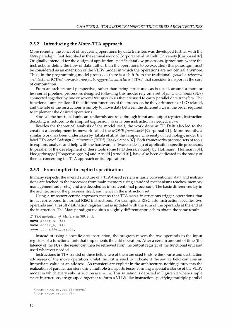
More recently, the concept of triggering operations by data transfers was developed further with theMove paradigm, first described in the seminal work of Corporaal et al. at Delft University [Corporaal 97].Originally intended for the design of application-specific dataflow processors, (processors where theinstructions define the flow of data, rather than the operations to be executed) this paradigm mustbe considered as an extension of the VLIW model in which the operations are not central anymore.Thus, in the programming model proposed, there is a shift from the traditional operation-triggeredarchitectures (OTAs) towards transport-triggered architectures (TTAs) that consider transport at the coreof computation.

From an architectural perspective, rather than being structured, as is usual, around a more orless serial pipeline, processors designed following this model rely on a set of functional units (FUs)connected together by one or several transport buses that are used to carry parallel data transfers. Thefunctional units realize all the different functions of the processor, be they arithmetic or I/O related,and the role of the instructions is simply to move data between the different FUs in the order requiredto implement the desired operations.

Since all the functional units are uniformly accessed through input and output registers, instructiondecoding is reduced to its simplest expression, as only one instruction is needed: move.

Besides the theoretical analysis of the model itself, the work done at TU Delft also led to thecreation a development framework called the MOVE framework2 [Corporaal 91]. More recently, asimilar work has been undertaken by Takala et al. at the Tampere University of Technology, under thelabel TTA-based Codesign Environment (TCE3) [Jääskeläinen 07]. Both frameworks propose sets of toolsto explore, analyze and help with the hardware-software codesign of application-specific processors.In parallel of the development of these tools some PhD theses, notably by Hoffmann [Hoffmann 04],Hoogerbrugge [Hoogerbrugge 96] and Arnold [Arnold 01], have also been dedicated to the study ofthemes concerning the TTA approach or its applications.

2.5.3 From implicit to explicit specification

In many respects, the overall structure of a TTA-based system is fairly conventional: data and instruc-tions are fetched to the processor from main memory using standard mechanisms (caches, memorymanagement units, etc.) and are decoded as in conventional processors. The basic differences lay inthe architecture of the processor itself, and hence in the instruction set.

Using a transport-centric approach means that TTA move instructions trigger operations thatin fact correspond to normal RISC instructions. For example, a RISC add instruction specifies twooperands and a result destination register that is updated with the sum of the operands at the end ofthe instruction. The Move paradigm requires a slightly different approach to obtain the same result:

// TTA equivalent of MIPS: addi $t0, 4, 3;move adder_a, #3;move adder_b, #4;move t0, adder_result;

Instead of using a specific add instruction, the program moves the two operands to the inputregisters of a functional unit that implements the add operation. After a certain amount of time (thelatency of the FUs), the result can then be retrieved from the output register of the functional unit andused wherever needed.

Instructions in TTA consist of three fields: two of them are used to store the source and destinationaddresses of the move operation whilst the last is used to indicate if the source field contains animmediate value or an address. As transfers are explicit in the architecture, nothings prevents therealization of parallel transfers using multiple transports buses, forming a special instance of the VLIWmodel in which every sub-instruction is a move. This situation is depicted in Figure 2.2 where simplemove instructions are grouped together to form a VLIW-like instruction specifying multiple parallel

2http://www.cs.tut.fi/~move/3http://tce.cs.tut.fi/

16

2.5. TRANSPORT TRIGGERED ARCHITECTURES

sourcedesti

Bus 1 slot

...sourcedesti

Bus 2 slot

sourcedesti

Bus n slot

Figure 2.2: VLIW instruction word specification in TTA.

transfers. In this case not only must the data transports be rendered explicit, but also the buses to beused. Thus, almost every detail of the architecture is exposed and made available to the programmer’sview, and hence the compiler.

2.5.4 Exposing various levels of connectivity

Figure 2.3, which is based on the same graphical representation used by Corporaal in [Corporaal 99],depicts a schematic view of an hypothetical TTA processor containing four transport buses and fivefunctional units. The network controller that is present in the figure can be considered as the TTAequivalent of a fetch unit as it is in charge of controlling the pipelining of data transports between theFUs. These latter interface to the interconnection network using sockets, units that can possess eitherread or write ports. They respectively correspond to multiplexers and to demultiplexers that are usedto put information to and from the FUs. Optionally, the FUs can implement a register in the interfaceendpoint with the sockets.

FU FU FU

FU FU

Net

wo

rkco

ntr

olle

r

Interconnectionnetwork

Socket

Read port

Write port

Figure 2.3: General architecture of a TTA processor.

Regarding the interconnection network, its functionality can be implemented in different waysas long as the displacements required by the application are allowed. When considering processorsembedded in a single-chip configuration, it can be achieved using a traditional shared bus structurebut nothing prevents implementations that specify transports outside the boundaries of the chip, aswe will demonstrate in chapter 10.

However, if we limit our current discussion to single-chip configurations, connectivity can rangefrom full-custom connectivity to full connectivity. In the first case, the interconnection network istailored for a specific application: this is the case in Figure 2.3 where four concurrent transports arepossible but only under certain specific circumstances. This yields a lightweight implementation alongwith a reduced bus load, at some expense in versatility. In case of full connectivity, the cost in terms ofhardware is higher but code generation is simplified. We will analyze further this issue in section 4.2,when we consider the implementation challenges and opportunities that such an architecture poses forthe development of a C compiler, but we can already mention that the task of the compiler in a TTAsystem consists of reducing the number of cycles for each data displacement, within the constraints ofa given connectivity.

17

CHAPTER 2. TOWARDS TRANSPORT TRIGGERED ARCHITECTURES

2.6 TTA advantages and disadvantages

If the main advantage of the TTA approach resides in its clear exposition of transport buses, italso enables specific optimizations. Notably, based on the observations that operations results areseldom used more than once and that they are often used immediately after their computation[Lozano 95,Martin 97,Cruz 00], it might be interesting in some cases to devise a new solution to reducethe importance of the monolithic structure that constitutes the register file (RF). This is particularly truein VLIW because of the inherent cost, in terms of material, to implement such structures when multipleaccesses are required, as pointed out in [Corporaal 97, p. 102]:

“VLIWs with K FUs need 3K ports on the RF: 2K read ports and K write ports4. Theseports are needed because in the worst case situation each FU needs to perform two readsand one write on the RF simultaneously.”

In TTA, because every displacement and location must be explicit, it is no longer required tostructure registers in a file, nor to group arithmetic operators into an ALU. Thus, these structures canbe distributed among the different FUs that compose the processor and we will expose notably inchapter 6, the advantages that can be drawn from such a situation. TTA processors offer thus the sameflexibility as VLIW processors in the sense that FUs can be added or removed very easily. However,where VLIW processors have to face a dramatic increase in terms of complexity to implement therequired RF ports and the bypass logic, TTA processors enable a different approach in which this issueis simplified.

2.6.1 Architecture strengths

The TTA approach, in and for itself, does not imply high performance. However, several argumentsin its favor have been proposed, notably in [Corporaal 97, Nikhil 89, Hoogerbrugge 94] where theinterested reader will find a more detailed perspective on the subject. In the context of this thesis, weretained the following pertinent elements:

1. ModularityFrom an architectural point-of-view, the Move model allows a distinct separation between thethree main components at the core of the processor, namely:

• Computation, with the use of distributed functional units instead of regrouped operators.Thus, arithmetic operators are not necessarily regrouped in an arithmetic and logic unit (ALU).

• Storage, with registers not necessarily tied to register files.

• Communication, with a flexible routing infrastructure instead of a rigid data path.

In addition, each FU is connected to the other components of the system by means of a unifiedinterface: the socket. From a designer’s perspective, the modularity offered by this commoninterface is manifold.

Firstly, it is interesting because it inherently implies that every component of a processor –functional units but also bus or memory interfaces – can be designed and tested separately as adistinct block. This allows a simplified generation of work units, which in turn simplifies workdistribution in a team.

Secondly, testability is also increased because each component is independent, which translatesinto the fact it can be fully and independently tested before being integrated with the rest of theprocessor.

Thirdly, in the context of reconfigurable computing, it becomes possible to automate the designof processors by putting together different compatible building blocks that share a commoninterface.

4Assuming a VLIW with a shared RF, and FUs with two source and one destination operands.

18

2.6. TTA ADVANTAGES AND DISADVANTAGES

A supplementary advantage of FU separation resides in the fact that FUs can possess multipleoutputs and inputs, enabling any functionality to be implemented easily, even if it requires morethan two inputs or produces more than one output.

Note that the idea of a modular design that uses various building blocks to create a processor hasalso been used in other architectures, such as [Rabaey 98] or [Hartenstein 99].

2. FlexibilityThe explicit definition of the interconnection network that links the different FUs and the fact thatonly few constraints are imposed on its implementation allow a considerable amount of flexibilityin its design. Notably, the architecture allows the number but also the nature (shared, external,ad-hoc, . . . ) of the buses used to transport instructions to be changed at will. Furthermore, aslong as the implemented FUs adhere to the socket interface, there are no restrictions on how theyare implemented. As a result, they can be easily pipelined and exhibit different latencies.

Of course, VLIW and EPIC architectures also allow multiple operations to be performed inparallel but the addition or removal of any operation (which could roughly correspond to aTTA FU) requires the interconnection network and the register file to be changed accordingly.This process is much simpler with TTA processors thanks to a more marked separation betweentransport and computation.

3. ScalabilityTo keep the hardware footprint as low as possible, a TTA processor can be reduced to its minimalform because unused FUs can be easily removed (see section 3.1). Similarly, adding new FUsis also possible, for example to cope with special processing demands, such as a fast Fouriertransform (FFT) unit.

In addition, because only move operations have to be considered, changing the processor doesnot require the software tools, such as the assembler, to be changed to accommodate differenthardware configurations. Furthermore, binary compatibility can be preserved between differentCPU revisions, even when new FUs are added.

We will see the full range of these advantages when we will consider the development of ad-hocFUs in chapter 6.

4. EfficiencyFrom a strict hardware perspective, there are several advantages in implementing a TTA proces-sor:

• Trivial decoding. Because only a single instruction is present, decoding can be kept verysimple and resources freed for other purposes.

• Fine-grained instruction level parallelism (ILP) is achievable through VLIW-encoded instruc-tions.

• Power savings. In addition to the advantage, in terms of energy, of having a simple decodinglogic, TTA processors can implement clock gating techniques to save power by turning offunused FUs. Moreover, the fact that the data transports are determined at compile timeallows fine-grained power optimizations techniques to be used.

• Limited register file traffic. This advantage comes from the fact that a register file is not strictlyrequired, since a distributed version can be implemented by directly moving data from oneFU to another, taking advantage of the fact that many produced results are used only onceand hence do not need to be allocated to a general purpose register. The outcome of thisdistribution is that the traffic normally passing through the RF (which may constitute abottleneck) is spread over the different FUs.

• Elimination of monolithic structures. By splitting the register file and the ALU in different FUs,resource conflicts are reduced during instruction scheduling, which enables an increase inconcurrency.

19

CHAPTER 2. TOWARDS TRANSPORT TRIGGERED ARCHITECTURES

Software related advantages, implemented as compiler optimizations, will be discussed in detailin section 4.3.4.

5. Hardware neutral perspectiveThe fact that the architecture handles the functional units as “black boxes”, i.e. without anyinherent knowledge of their functionality, implies that the internal architecture of the processorcan be described as a memory map which associates the different possible operations with theaddresses of the corresponding functional units.

We define this hardware viewpoint as hardware neutral because in this situation, the hardwaredoes not need to consider what the transports do, but only where to get and put the data, This isof particular interest for the development of the software tools (more on this in chapter 5).

2.6.2 Architecture weaknesses

Of course, the architecture also presents some drawbacks, which can be categorized into three differentcategories:

1. Code complexityThe major problem with Move processors resides in the fact that programming such processorsrequires a completely different approach from any other architecture. The programmer’s modelthat directly derives from the hardware consists only of move instructions, a narrow perspectivethat forces to think in terms of displacements and requires a long adaptation phase. In otherwords, because the programmer has to manage everything in terms of displacements, assemblyprogramming becomes very difficult.

Of course, the presence of a compiler solves this particular issue. The problem is that Movecompilers are scarce, probably because of the complexity of generating efficient code in thiscontext. In fact, Move processors compilers not only must face the same difficulties tackledas VLIW compilers, but must also be able to handle the specific optimizations allowed by thearchitecture.

2. Expensive exception handlingIf the disappearance of register files as monolithic structures presents some advantages, it rendersexception handling and context saving very expensive. The reasons for this are simple: in theworst case, all the registers that are distributed among the different processor FUs must besaved and restored when an exception occurs. This could generate a prohibitive cost, notablybecause every register present must be made readable and writable to the architecture (hence,fully accessible on the buses). In addition, the problem of pipelined FUs (that present differentlatencies) must also be tackled when an exception or an interrupt occur.

The combination of these two issues leads to problems with context switching, which is requiredfor example by preemptive multitasking, and interrupts. This makes some people concludethat it is “currently considered not feasible” [Jääskeläinen 07] to port a multitasking OS for suchan architecture. Yet, solutions exist (see for example [Corporaal 97, chapter 10]) to implementexceptions support in TTA processors, even if they can be quite expensive.

3. Code sizeLarge instructions translate into large code, because the more parallel transport buses are present,the more data displacements must be specified. EPIC implementations solve the problem bycompressing unused instruction slots that would have otherwise have been filled with nopoperations.

Similarly, code compression is applicable to TTA processors, with the advantage that it reducesmemory needs and also energy consumption (see [Heikkinen 05]). Nevertheless, general codedensity is lower with Move processors than with traditional approaches [Myers 81, pp. 463–494]and [Corporaal 97, p. 243], which translates into higher memory requirements.

20

2.7. A FLEXIBLE OPERATION-SET

The Move model has, until now, been mainly restricted to the academic field. To our knowledge, theonly notable industrial exception is the Maxim’s MaxQ processor5 [Maxim 04], which takes advantageof the clock-gating capabilities of the architecture to reduce power consumption to very low levels (theMAXQ200, a 16-bit microcontroller, can thus reach 3.5 MIPS/mA).

This relative lack of interest in the architecture is probably explained by the general absence ofefficient and mature software tools that can tackle the programming difficulty of such processors andattain the performance of existing solutions.

2.7 A flexible operation-set

Aside from the advantages and disadvantages that have just been described and that aim at character-izing TTA processors from an architectural or implementation point-of-view, we consider that it is ofparticular interest to also examine TTAs from a programmer’s perspective.

Even if the architecture uses only one kind of instruction, it is clear that TTA processors are able toperform more than one type of operation. In this context, an operation can be defined as:

Definition An operation is the set of modifications, in terms of the internal state of a processor, resultingfrom a single instruction.

Even for RISC processors, an instruction covers less than its corresponding operation. Let usconsider the following MIPS instruction:

add r3, r1, r2;

This instruction has three effects. First, it changes the state of the r3 register to correspond to thesum of the registers r1 and r2. Second, the flag register of the processor is also updated to reflectpotential overflows, the sign bit of the result, etc. Third, the PC value is updated to point to the nextinstruction. These three effects, following the aforementioned definition, correspond to the operationconducted. Keeping that in mind, it then becomes possible to define the operation set of a processor.

Definition The operation set of a processor is the set of every operation spanned by the instruction setof the processor.

In traditional architectures, the operation set does not play a very important role because it closelyresembles the instruction set, the differences consisting mainly of the side effects of the instructions6. Thesituation is different for TTA architectures. In fact, from an architectural point-of-view, the situationcan be seen as if such processors were programmed only with side effects.

Even if the instruction set of a TTA processor is reduced to its simplest expression (it is a singletonwhen not considering the parameters of the move instruction), its corresponding operation set spansthe whole range of operations conducted by other processors. As such, TTA processors can alsobe considered as universal Turing machines that can carry any kind of computation using only oneinstruction.

In the context of this work, the existence of a dichotomy between instruction and operation setrepresents an undeniable advantage. In fact, this separation allows drastic changes in the processoroperation set that would be much more difficult to obtain in every other architecture considered.

2.8 TTA and soft-cores

In parallel to all VLSI circuits, reconfigurable logic has also dramatically improved in the last years:FPGAs, for example, have become from a quantitative perspective, large enough to implement com-plete embedded processors. This has led to the appearance of a certain number of soft-cores, i.e.

5http://www.maxim-ic.com/appnotes.cfm/appnote_number/32226Such as flag settings or interrupt triggering.

21

CHAPTER 2. TOWARDS TRANSPORT TRIGGERED ARCHITECTURES

processors that are proposed as software components that can then be realized into hardware withinprogrammable logic circuits.

Some of these soft-cores are fully open-sourced, which is the case for example for the Leon3-SPARCprocessor7, while some are only available as IP modules with a more limited configurability. In this lastcategory, every major company in the reconfigurable logic industry has proposed specific processors(MicroblazeTM8 for Xilinx, NiosTM9 for Altera, to cite only two). All these soft-cores share the capabilityto be configured to implement different modules such as UART communication modules, DMA orJTAG controllers, various memory interfaces. . . . In addition to these modules, which are often pre-defined, there also exists the possibility to implement VHDL components that can then be used bythe processor to generate ad-hoc processors. Inside this plethora of possibilities, some researcherseven propose dynamically reconfigurable processing elements, for example to accelerate some kinds ofcomputation [Campi 07, Mucci 08].

The aforementioned processors are generally based on a RISC instruction set and access the variousperipherals through a dedicated memory zone. One advantage of TTA processors in this context isthat, because their whole operation is based on a memory map, i.e. each operation is implemented inan FU and accessible via a data displacement inside the memory space of the CPU, the architecture iscompletely regular and does not necessitate special mechanisms to implement an arbitrary number ofFUs. As such, they are very good candidates for a configurable soft-core implementation.

Of course, from an hardware point of view, it is also possible to use the same memory mappingmechanism to perform operations in a RISC or VLIW architecture. However, the flexibility attained inthe TTA approach, where the functional units are really pluggable, is undeniable, as we will see in thenext chapters.

2.9 Conclusion

After having described the general strengths and weaknesses of TTA processors, it should be fairly ob-vious that they possess key capabilities in the context of our bio-inspired approach. First, the versatilityof the TTA paradigm fulfills all the requirements for the synthesis of ontogenetic, application specificinstruction set processors (ASIPs), that can assemble from basic building blocks. More specifically, thepossibility of specializing the operation set with ad-hoc functional units enables to adapt the processorto the application while keeping the overall structure of the processor – fetch and decode unit, busstructure, etc. – unchanged. Moreover, the fact that architecturally only data transports are visibleseparates functional units (where computation is done) from their scheduling (when the computationis done).

7http://www.gaisler.com8http://www.xilinx.com/products/design_resources/proc_central/microblaze.htm9http://www.altera.com/products/ip/processors/nios/nio-index.html

22

Bibliography

[Agerwala 82] T. Agerwala. Data Flow Systems: Guest Editors’ Introduction. Computer, vol. 15, no. 2,pages 10–13, 1982.

[Arnold 01] Marnix Arnold. Instruction set extension for embedded processors. PhD thesis, DelftUniversity of Technology, 2001.

[Baron 08] Max Baron. VLIW: Failure or Lesson ? Microprocessor Report, June 2008.

[Campi 07] Fabio Campi, Antonio Deledda, Matteo Pizzotti, Luca Ciccarelli, Pierluigi Rolandi,Claudio Mucci, Andrea Lodi, Arseni Vitkovski & Luca Vanzolini. A dynamicallyadaptive DSP for heterogeneous reconfigurable platforms. In Proceedings of the conferenceon Design, automation and test in Europe (DATE’07), pages 9–14, San Jose, CA, USA,2007. EDA Consortium.

[Chang 91] Pohua P. Chang, Scott A. Mahlke, William Y. Chen, Nancy J. Warter & Wen meiW. Hwu. IMPACT: an architectural framework for multiple-instruction-issue processors.SIGARCH Computer Architecture News, vol. 19, no. 3, pages 266–275, 1991.

[Cocke 90] John Cocke & Victoria Markstein. The evolution of RISC technology at IBM. IBMJournal of Research and Development, vol. 34, no. 1, pages 4–11, 1990.

[Colwell 88] Robert P. Colwell, Robert P. Nix, John J. O’Donnell, David B. Papworth & Paul K.Rodman. A VLIW architecture for a trace scheduling compiler. IEEE Transactions onComputers, vol. 37, no. 8, pages 967–979, 1988.

[Corporaal 91] Henk Corporaal & Hans (J.M.) Mulder. MOVE: a framework for high-performance pro-cessor design. In Supercomputing ’91: Proceedings of the 1991 ACM/IEEE conferenceon Supercomputing, pages 692–701, New York, USA, 1991. ACM.

[Corporaal 97] Henk Corporaal. Microprocessor Architectures: From VLIW to TTA. John Wiley & Sons,Inc., New York, USA, 1997.

[Corporaal 99] Henk Corporaal. TTAs: missing the ILP complexity wall. Journal of Systems Architec-ture, vol. 45, pages 949–973, 1999.

[Cruz 00] José-Lorenzo Cruz, Antonio González, Mateo Valero & Nigel P. Topham. Multiple-banked register file architectures. SIGARCH Computer Architecture News, vol. 28,no. 2, pages 316–325, 2000.

[Dennis 88] J. B. Dennis & G. R. Gao. An efficient pipelined dataflow processor architecture. In Super-computing ’88: Proceedings of the 1988 ACM/IEEE conference on Supercomputing,pages 368–373, Los Alamitos, CA, USA, 1988. IEEE Computer Society Press.

[Flynn 99] Michael J. Flynn, Patrick Hung & Kevin W. Rudd. Deep-Submicron MicroprocessorDesign Issues. IEEE Micro, vol. 19, no. 4, pages 11–22, 1999.

[Grafe 89] V. G. Grafe, G. S. Davidson, J. E. Hoch & V. P. Holmes. The Epsilon dataflow processor.SIGARCH Computer Architecture News, vol. 17, no. 3, pages 36–45, 1989.

23

BIBLIOGRAPHY

[Halfhill 08] Tom R. Halfhill. Intel’s Tiny Atom – New low-power microarchitecture rejuvenates theembedded x86. Microprocessor Report, vol. 1, pages 1–13, April 2008.

[Hartenstein 99] Reiner W. Hartenstein, Michael Herz, Thomas Hoffmann & Ulrich Nageldinger.Mapping Applications onto Reconfigurable Kress Arrays. In FPL ’99: Proceedings of the9th International Workshop on Field-Programmable Logic and Applications, pages385–390, London, UK, 1999. Springer-Verlag.

[Heikkinen 05] J. Heikkinen, A. Cilio, J. Takala & H. Corporaal. Dictionary-based program compressionon transport triggered architectures. In IEEE International Symposium on Circuits andSystems (ISCAS’2005), vol. 2, pages 1122–1125, May 2005.

[Hennessy 03] John L. Hennessy & David A. Patterson. Computer Architecture: A QuantitativeApproach. Morgan Kaufmann, third edition, 2003.

[Hoffmann 04] Ralph Hoffmann. Processeur à haut degré de parallélisme basé sur des composantes sérielles.PhD thesis, École Polytechnique Fédérale de Lausanne, 2004.

[Hoogerbrugge 94] Jan Hoogerbrugge & Henk Corporaal. Transport-Triggering vs. Operation-Triggering.In Proceedings of the 5th International Conference Compiler Construction, pages435–449, January 1994.

[Hoogerbrugge 96] Jan Hoogerbrugge. Code generation for Transport Triggered Architectures. PhD thesis,Delft University of Technology, February 1996.

[Huck 00] Jerry Huck, Dale Morris, Jonathan Ross, Allan Knies, Hans Mulder & Rumi Zahir.Introducing the IA-64 Architecture. IEEE Micro, vol. 20, no. 5, pages 12–23, 2000.

[Jääskeläinen 07] Pekka Jääskeläinen, Vladimír Guzma, Andrea Cilio, Teemu Pitkänen & Jarmo Takala.Codesign toolset for application-specific instruction-set processors. In Reiner Creutzburg,Jarmo Takala & Jianfei Cai, editors, Proceedings SPIE Multimedia on Mobile Devices2007, vol. 6507. SPIE, February 2007.

[Johnson 91] William M. Johnson. Superscalar Microprocessor Design. Prentice Hall, 1991.

[Lipovski 75] G. Jack Lipovski & J.A. Anderson. A Micronetwork for Resource Sharing. In Microar-chitecture of Computer Systems, page 223, Nice, France, 1975.

[Lipovski 77] G. Jack Lipovski. On virtual memories and micronetworks. SIGARCH ComputerArchitecture News, vol. 5, no. 7, pages 125–134, 1977.

[Lozano 95] Luis A. Lozano & Guang R. Gao. Exploiting short-lived variables in superscalar processors.In Proceedings of the 28th annual international symposium on Microarchitecture(MICRO 28), pages 292–302, Los Alamitos, CA, USA, 1995. IEEE Computer SocietyPress.

[Martin 97] Milo M. Martin, Amir Roth & Charles N. Fischer. Exploiting dead value information. InProceedings of the 30th annual ACM/IEEE international symposium on Microar-chitecture (MICRO 30), pages 125–135, Washington, USA, 1997. IEEE ComputerSociety.

[Maxim 04] Maxim. Introduction to the MAXQ Architecture, Application Note 3222. http://pdfserv.maxim-ic.com/en/an/AN3222.pdf, 2004.

[McNairy 03] Cameron McNairy & Don Soltis. Itanium 2 Processor Microarchitecture. IEEE Micro,vol. 23, no. 2, pages 44–55, 2003.

24

BIBLIOGRAPHY

[Mucci 08] Claudio Mucci, Luca Vanzolini, Ilario Mirimin, Daniele Gazzola, Antonio Deledda,Sebastian Goller, Joachim Knaeblein, Axel Schneider, Luca Ciccarelli & Fabio Campi.Implementation of parallel LFSR-based applications on an adaptive DSP featuring a pipelinedconfigurable Gate Array. In Proceedings of the conference on Design, automation andtest in Europe (DATE’08), pages 1444–1449, New York, USA, 2008. ACM.

[Myers 81] Glenford J. Myers. Advances in Computer Architectures. Wiley-Interscience, 1981.

[Nikhil 89] R. S. Nikhil. Can dataflow subsume von Neumann computing? SIGARCH ComputerArchitecture News, vol. 17, no. 3, pages 262–272, 1989.

[Patterson 85] David A. Patterson. Reduced instruction set computers. Communications of the ACM,vol. 28, no. 1, pages 8–21, January 1985.

[Patterson 98] David A. Patterson & John L. Hennessy. Computer Organization and Design. MorganKaufmann, second edition, 1998.

[Petkov 92] N. Petkov. Systolic Parallel Processing. Elsevier Science Inc., New York, USA, 1992.

[Rabaey 98] J. Rabaey & M. Wan. An energy-conscious exploration methodology for reconfigurableDSPs. In Proceedings of the conference on Design, automation and test in Europe(DATE’98), pages 341–342, Washington, USA, 1998. IEEE Computer Society.

[Rau 89] B. Ramakrishna Rau, David W.L. Yen & Ross A. Towle. The Cydra 5 departmentalsupercomputer: design philosophies, decisions and trade-offs. IEEE Computer, vol. 22,no. 1, pages 12–35, 1989.

[Schlansker 00] Michael S. Schlansker & B. Ramakrishna Rau. EPIC: Explicitly Parallel InstructionComputing. Computer, vol. 33, no. 2, pages 37–45, 2000.

[Tabak 80] Daniel Tabak & G. Jack Lipovski. MOVE Architecture in Digital Controllers. IEEETransactions on Computers, vol. 29, no. 2, pages 180–190, 1980.

[van Eijndhoven 99] J. T. J. van Eijndhoven, F. W. Sijstermans, K. A. Vissers, E. J. D. Pol, M. J. A.Tromp, P. Struik, R. H. J. Bloks, P. van der Wolf, A. D. Pimentel & H. P. E. Vranken.TriMedia CPU64 Architecture. In Proceedings of the IEEE International ConferenceOn Computer Design: VLSI In Computers and Processors (ICCD’99), 1999.

25

Chapter 3

The ULYSSE processor

“Heureux qui, comme Ulysse, a fait un beau voyage,Ou comme cestuy-là qui conquit la toison,

Et puis est retourné, plein d’usage et raison,Vivre entre ses parents le reste de son âge !”

JOACHIM DU BELLAY, Les Regrets

TO EVALUATE the different trade-offs, design decisions, but also possible opportunities in termsof bio-inspiration, we have implemented a “soft-core” processor, named ULYSSE, that will be

used as a cornerstone of this thesis. An instance of the TTA model, ULYSSE implements transporttriggering along with different mechanisms to achieve a maximum flexibility along with a good levelof performance.

In this chapter, we will describe the general architecture of this processor and also discuss thedesign decisions taken during the implementation. The software aspects being discussed separatelyin the next chapter together with the performance analysis of the resulting processor, this chapterwill be devoted only to hardware-related issues. When pertinent, we will also compare our designdecisions with the MOVE32INT processor [Corporaal 93], the only other non-commercial instance ofMove processor that we are aware of.

Thus, the topics described in this chapter are the following: the chosen transport model (how dataare transported inside the CPU), how pipelining works at the transport level, and also at the functionalunit level. In addition to the operation of the processor itself, we will cover as well some interestingFUs that were developed in the context of this thesis. Finally, we will end our discussion regarding thehardware architecture with an analysis of further extensions that could be applied to the model.

3.1 Internal structure overview

ULYSSE is a 32-bit soft processor that follows the TTA approach. As such, it can be described in itsessence as a set of FUs linked together with an interconnection network. To implement such a processor,three main classes of components are required:

1. Interconnection networkIt connects the different FUs and allows the data to be moved from one point to another insidethe processor.

Its realization details will be described in section 3.4.

2. Fetch unitIt constitutes the entry point of the instructions inside the processor: it is in the fetch unit that theinstructions are decoded and where reside the registers that permit to determine and change theflow of the program, namely the program counter (PC) and the instruction register (IR).

27

CHAPTER 3. THE ULYSSE PROCESSOR

We will see in section 3.6 how it was realized and in section 3.8.2 how conditional jumps arehandled within the processor.

3. Functional unitsThey determine the operation set of the processor by implementing not only arithmetic operationsbut also more specific functionalities such as I/O operations1, external memory interface orgeneral purpose registers. All these FUs have in common their access method that consists ofaddressable locations that may optionally contain a register.We will detail, starting in section 3.7, the various FUs that we have developed in the context ofthis thesis.

Memoryunit

Interconnection network

Conditionunit

Arithmeticunit

Arithmeticunit

Fetchunit

PCIR

RegisterunitAddressable register

Arithmeticunit

Arithmeticunit

Figure 3.1: Overview of a minimal ULYSSE processor.

Thus, a schematic, minimal version of ULYSSE processor (depicted in Figure 3.1) is composed ofa fetch unit, a memory interface, some arithmetic and logic functional units, a condition unit and aninterconnection network to connect everything together. Depending on the application, it can alsoinclude a register unit containing only registers.

3.2 Simplified operation

As most of the hardware complexity has been transferred to the software side, the basic operation ofthe processor is quite simple. The fetch unit extracts from memory the instruction pointed to by theprogram counter and, after a trivial decoding phase, the address of the location serving as a sourceand the address of the destination location are placed on the interconnection network on two separatebuses.

Every FU possesses an internal address (in what we call the inner addressing space of the processor)that is permanently matched with the source and destination buses. When a match occurs, the FUknows that it is used in an instruction. In that event, it writes or reads the data bus (which is 32 bitswide) depending on the instruction. In the case of immediate values, the data bus is assigned to thefetch unit that extracts immediate values directly from the instruction. By replicating the mechanismseveral times over, it is possible to realize multiple displacements in parallel.

3.2.1 Operation example

Let us now examine the mechanisms that are used in a very simple operation consisting of summingtwo numbers, 5 and 4, and then accumulating the result with 5 twice. The corresponding RISC code isas follows:

addi $t0, zero, 5;addi $t0, $t0, 4;addi $t0, $t0, 5;addi $t0, $t0, 5;

1Such as network interface, display controller, general-purpose I/O pins (GPIOs), . . .

28

3.2. SIMPLIFIED OPERATION

Obtaining the same result with our processor requires a slightly different sequence of instructions.First, the operands to be added should be displaced to an adder FU which, after a certain amount oftime (the latency of the operator, noted λ, in clock cycles units), will make the result available at oneof its output. The result can then be retrieved and reused as an input of the adder FU the requirednumber of times. The corresponding code is as follows:

move adderA, #5;move adderB_t, #4;move adderB_t, adder_r;move adderB_t, adder_r;

AdderA AdderB_t

+

Adder_r

SourceDestinationData

Address = 0 Address = 1

Address = 2

Interconnection bus

PCSrc = 2, Dest = 1

Dest = 0, Data = 5Dest = 1, Data = 4Src = 2, Dest = 1

+

Bus interface Bus interface

1

Instruction memory

Fetch unit Adder FU

Figure 3.2: Schematic TTA adder example.

The operation of the program is represented in Figure 3.2, which depicts how the instructions, whichcorrespond to displacements addresses, are fetched from a memory before being put on dedicatedbuses. In this example, the first move specifies to transfer the immediate value 5 to address 0, whichis the AdderA register. The second displacement indicates that the immediate value 4 must be putinto address 1 (register AdderB_t): here the “_t” suffix indicates that writing to this register triggersthe operation (see next section), which in this case signifies that the value 9 will be put into registerAdder_r. At the end of the execution of this program, Adder_r will store the value 19.

Several remarks can be made concerning this program. We can notably notice that it was possibleto displace the value from the output register to the operand register without going through anintermediary one. Moreover, the final result remains in the output register of the adder unit until anew operation is triggered, which in this situation corresponds to writing to a special register. Otherschemes are possible as we will discuss in the next section.

3.2.2 Triggering schemes

If data transports trigger operations in the chosen architecture, several triggering schemes can be used.In other words, different techniques can be used to determine when operations occur following a datatransfer.

Hoffmann’s taxonomy of triggering schemes [Hoffmann 04, p. 87–88] distinguishes several policiesthat define under which conditions an operator should start a computation and under which conditionsa result should be produced. Besides the concept of triggering operand defined by Corporaal in[Corporaal 97], he defines the concept of neutral operand as an operand that does not produce visibleresults2. Such operands are rather rare and he cites the example of the data memory where the address

2The original text is “C’est l’absence de résultat visible qui justifie le qualificatif de neutre.” [Hoffmann 04, p. 87].

29

CHAPTER 3. THE ULYSSE PROCESSOR

to access the data is first stored before another input is used to define the operation to be carried out.In total, we distinguish at least four different triggering schemes:

1. Co-triggeringThe FU realizes its corresponding operation when all the required operands have been updated.

2. Triggering operandThe update of specific operands (which can be unique or not) triggers an operation, regardless ofthe state of the other operands. This triggering scheme is useful for instance to be able to modifiynon-triggering operands whilst keeping the output valid. This is the scheme used in the exampleof the previous section.

3. Triggering inputAn input of the FU is used only to trigger operations. This method is quite similar to thesecond but allows a bit more flexibility because every input operand is then equivalent (with noside-effect).

4. Triggering readAn operation can be triggered when a particular output (or input) of an FU is read. This can beused for example to realize a FIFO memory FU, where a value is popped everytime it is read.

These different schemes are not exclusive and can be mixed together in a CPU to accommodatevarious needs. In the described processor, the triggering operand is almost always used.

3.3 Different CPU versions

At the time of writing this thesis, three different version of ULYSSE have been implemented on threedifferent hardware platforms. All share the general TTA organization that was presented before andtheir main differences reside in the peripherals they contain, notably due to the requirements of thedifferent hardware platforms targeted.

Historically, the first version developed targeted a PCI board hosted on a PC computer, on a Xilinxr

VIRTEXTM II-3000 FPGA. Because of the relative large size of that FPGA, this first version makes useof embedded memory and can realize two move operations in parallel. For this reason, it is called theVLIW version. Despite this unique feature, this version is of little interest because its development wascompletely stopped at an early stage for reasons that will be explained in section 3.4.1.

The second version of the processor is a standalone version and is depicted in Figure 3.3, whichdetails how the different components of the processor are interconnected but also how it interfaceswith the outside world. This version of the processor targeted small FPGAs and for this reason it usesa SRAM controller along with a serial code-loader. It can also include one or several general purposeI/O (GPIO) controllers to interact with external hardware. Mainly developed as a debugging platform,it was implemented on a Xilinxr SPARTANr 3 3XCS200 FGPA board.

The last version is called the cellular version because it targeted our cellular hardware substrate,discussed later in chapter 7. It is based on the standalone version but with the additional constraint thatit is used in a multiprocessor environment in which it must communicate using a high-speed networkinterface that also serves to update the CPU code. Additionally, it also possesses an interface to a RGBled display. It is the most complete and most tested version of ULYSSE and, unless stated otherwise,we mainly discuss this version even if it is somewhat interchangeable with the standalone version.

3.4 Interconnection network

ULYSSE is programmed using only data transports from FU to FU. They take place on the interconnectionnetwork of the processor. Among the different compromises between performance and size that areavailable to implement the interconnection network, ULYSSE uses a shared bus topology with fullconnectivity, on which FUs are simply plugged in. This means that the interconnection network is

30

3.4. INTERCONNECTION NETWORK

Interconnection busPr

ogra

mm

ing

Mem

ory

Optional units

DCM

Resetmanager

Fetchunit

SRAMunit

Debugunit

GPIOunit

ALUFU

CondFU

ConcatFU

RegisterFU

ShiftFU

Figure 3.3: Detailed view of the ULYSSE processor in its standalone version.

composed of three different buses that contain the source address, the destination address and thedatum to be transported. This network appears in Figure 3.2 or in Figure 3.6.

Even if this kind of connectivity is more expensive from an hardware perspective, it remains rela-tively simple to implement whilst proposing an adequate performance. Scheduling is also simplifiedbecause full connectivity enables displacements from any register to any other register in the CPU.Consequently, code generation is simpler.

In the MOVE32INT processor, a customizable version of the interconnection network was im-plemented, using sockets to add or remove connections from a particular FU to a transport bus. Byanalyzing different connectivity configurations, the influence of the connections on various aspectssuch as processor performance or size could be determined.

Another difference between the two processors lies in the number of parallel transport buses. InMOVE32INT processor, up to four data displacements in parallel can be specified whereas only twoare possible in our case with the VLIW version.

3.4.1 Single slot instructions

The use of multiple slots instructions as proposed in the VLIW version was abandoned in the twomajor implementations – standalone and cellular – we are discussing here. The decision to focus onthe implementation of a single move slot per instruction was made for several reasons:

Difficult programming in the absence of an adequate compiler The ULYSSE processor developmentstarted several years ago, at the very moment we began working on this thesis. At that time,several questions were still open. Notably, the existence of a valid compiler for that newbornprocessor was not certain. Consequently, we decided not to rely too much on this hypothetical

31

CHAPTER 3. THE ULYSSE PROCESSOR

development but we left, as much as possible, the door open to future developments. Thus, aworking version of ULYSSE with parallel displacements was developed but the advantages wereonly slim compared to a non-parallel version, due to the lack of an adequate compiler but alsobecause assembler programming by hand was too difficult. Two main reasons explain this:

• Dependencies checking between the instructions is very difficult to do by hand and is thesource of many errors.

• Writing an optimized program for multiple displacements (i.e. VLIW instructions) requirestwo passes on the code, one for writing what we want the processor to do followed by asecond where the instructions are moved to free slots. The resulting code becomes then verydifficult to read because pieces of code that should normally be together are disseminatedin different slots.

Because of these reasons and the fact that enabling multiple parallel displacements was not ourtop priority, we decided at that time not to continue in that direction.

During the following years it turned out that, with the help of Michel Ganguin who realizedhis master thesis under my supervision, a working version of GCC was made available for thisprocessor (see section 4.2). Of course, due to the huge complexity of such a piece of software,some bugs are still present but they remain completely bearable under the assumption that itis still under ongoing development. However, even if a basic compiler exists, optimizing it soit would be able to use the parallel displacement slots in an intelligent way goes beyond thesubject of this thesis. In fact, the subject was treated in detail by Hoogerbrugge in his PhDdissertation [Hoogerbrugge 96].

Reduced memory size Because the target processing elements we focus our attention on are small-sized, embedded processors, the amount of memory they possess remains relatively modest.Considering the fact that Move code is already less dense than standard code (see [Myers 81, pp.463–494] and [Corporaal 97, p. 243]), it is not realistic to implement enough slots so that VLIWcan be interesting from a performance perspective. Moreover, more slots would even morecomplicate the situation explained in the previous point.

nop instructions and wasted memory The aforementioned limited memory problem also impliesthat space can not be wasted by the insertion of nop instructions to fill the unused slots, whichwould be necessarily the case without optimized and automatic methods to fill them at compiletime. Of course, solutions exists to compress VLIW instructions (for instance [Xie 01, Lin 04]),but their implementation would not change anything to the problem of the lack of an efficientcompiler.

3.4.2 Instruction format and inner addressing

One of the advantage of the Move architecture is that it does not necessitate complex decoding becauseonly one instruction exists, with two variants:

1. move address, address

2. move address, immediate value

The nop “instruction” can be added to these two instructions by defining it as a displacement fromaddress 0 to address 0. This formal definition can also be extended by noting that any displacement toa non-existing address also constitutes a nop instruction, a fact that we will use notably for testing (seesection 5.1).

In summary, each instruction must code the following elements:

• a source address;

• a destination address;

32

3.5. A COMMON BUS INTERFACE

• a flag to indicate if an instruction contains an immediate value or two addresses.

In the standalone and cellular implementations, immediate values are 16 bits3 wide whereas sourceand destination addresses are coded with 15 bits each4. The immediate flag uses one bit. Thus, thespecification of one displacement requires 32 bits with an immediate value and 31 for register-to-register moves. In the latter case, one bit of padding is used to align on the 32 bits boundary word.This gives the following instruction format (P being the padding bit):

Immediate→ Address : 1 | DDDD . . .DDDD︸ ︷︷ ︸15 bits dest.

| IIII . . .IIII︸ ︷︷ ︸16 bits imm. value

(3.1)

Address→ Address : 0 | DDDD . . .DDDD︸ ︷︷ ︸15 bits dest.

| SSSS . . .SSSS︸ ︷︷ ︸15 bits source

| P (3.2)

The inner addressing space (the space that can be addressed with these 15 bits) has been separatedinto 1024 segments (one per functional unit), each permitting 32 addresses that correspond to themaximal number of interfaced register per functional unit. This paginated access was implementedin order to reduce the complexity of the bus interface (see section 3.5) and yields to the followingpaginated representation:

(base, page) with base ∈ [0, 1023] and page ∈ [0, 31]

3.5 A common bus interface

Base address NReg

Matchlogic

Generic parameters

Figure 3.4: Schematic of the common bus interface.

3We will discuss in section 3.8.1 how immediate values that do not fit this range can be used.4The VLIW implementation uses shorter inner addressing space with only 9 bits for immediate values and 8 bits for source

and destination.

33

CHAPTER 3. THE ULYSSE PROCESSOR

An important building block of the processor is the bus interface (Figure 3.4), or socket, that connectsevery FU to the interconnection network of the processor.

In our architecture, one important feature the bus interface had to possess is scalability, in the sensethat the number of input or output registers had to be changed easily to accommodate different needswithin the FU. By developing a standardized interface (the VHDL interface is reported in the annex,section A.1), we managed to achieve independence between the function realized and its interfacewithin TTA. Using the interface, any VHDL component can be easily integrated inside ULYSSE: itsuffices to instantiate the bus interface and specify the number of interface ports (or registers) used toconnect to the system5.

The interface shown in the figure also provides signals (re_regs and we_regs) that indicate,using a one-hot bit encoding, when a register is accessed for reading or writing. This allows for instanceto implement complex triggering schemes based on the fact that a particular location has been read orwritten.

The interest of using a paginated addressing scheme appears clearly: thanks to that, the comparisonwith the FU address uses only BaseRange bits (i.e. 10 bits in the two main implementations).

Annexed listing (Listing A.2, p. 210) provides an example of a very simple FU – used to concatenatetwo immediate, 16 bit values to form a complete 32 bit word – that depicts the basic interface andhow it is used in a real example to provide a simple, yet powerful interface between ULYSSE and itsfunctional units.

3.6 The fetch unit

The primary role of the ULYSSE processor’s fetch unit is to schedule the global operation of theprocessor, which is summarized by its state machine (Figure 3.5).

Debug Stall

ExecuteFetch

Halt

default

(DEST|SRC)==BUSY

defaultNOT Halt

Halt

(DEST|SRC)==BUSY

Rst

Figure 3.5: Fetch unit state machine.

The fetch unit realizes three main operations:

1. Instruction fetchingThe fetch unit is primarily a load unit which is responsible of requesting new instructions fromthe memory. To fulfill this task, it does not include directly a memory controller but it interfaceswith a memory unit (see section 3.7) that handles the low-level transfers with the memory; thisdecoupling enables to use different kinds of memory very easily.

5The maximum number of registers that can be used depends on the number of bits used in the coding of instruction, eachregister corresponding to a page in the base–page terminology (see section 3.4.2). In the case depicted here, 32 registers can beused per FU.

34

3.6. THE FETCH UNIT

The instructions are fetched from addresses stored in the program counter (PC) of the fetch unit.This register is automatically updated to point to the next instruction every time one completes.

The PC register also belongs to the inner addressing space and can also be changed from theFUs, a mechanism used for realizing jumps. Conditional jumps use the standard mechanism ofchanging the PC with a special register (the condition register) that indicates, based on its value,if the jump should be taken or not. Different kind of conditions are possible and are computed inanother FU, the condition unit (see section 3.8.2).

2. Instruction decodingExecute directly follows the Fetch, with no cycle dedicated to the Decode phase. This simplificationwas made possible thanks to a trivial decoding logic that could be integrated at the beginning ofthe Execute phase. Because of its short execution time – basically, decoding in this case is just amultiplexer – this does not penalize the final working frequency.

In our processor, we chose to decode the instructions in a centralized way. In that, it differs fromthe MOVE32INT processor in which the decoding has been distributed into the FUs themselves,the instructions being passed directly to every FU.

3. Transport schedulingWhen the instructions have been decoded, they are executed by the FUs and, after a clock cyclein the normal case, the next instruction is fetched.

An exception to this scheme is that, when required, the processor can be put in Debug mode,which corresponds to a pause in the execution flow. This can be used for debugging purposes andwe used that halt mechanism during the development of an in-circuit debugger (see section 5.3),which can be used to examine and change all the processor’s registers, to execute instructionsstep-by-step, . . . . In this mode, instructions are not fetched using the normal scheme and theautomatic update of the fetch unit registers (the automatic PC increment, for example) is inhibited.

Interconnection bus

Bus interface

Conditionlogic

Statemachine

IR 0 IR

Immediatevalue

RET

PC

Memory interface

External interface

Figure 3.6: The fetch unit.

35

CHAPTER 3. THE ULYSSE PROCESSOR

In the schematic overview of the fetch unit, shown in Figure 3.6, it is worth noting the presenceof an instruction register (IR), even in the absence of a dedicated decoding phase6. Even if it is notstrictly necessary during the normal operation of the processor, the IR is loaded at the same timeas the instruction is executed. However, it is not used to assign the source and destination buseswhich are assigned, like immediate values, directly from the output of the memory unit. Its presenceis justified because when the processor is stalled or in debug mode, the memory interface must bereleased. During that time, buses might need to maintain their value, which is done by using the valuestored in the IR. Finally, as the IR is present in the memory map of the processor, it can be used asa source or as a destination like any other register; this permits “exotic” operations to be performed,which can be used for example in the debugger described in section 5.3.

In addition to the PC and IR registers, the fetch unit also contains another register that is accessiblein the inner addressing space: the return address register (RET). The RET register can be used to storethe return address of the caller function during procedure calls. It does not implement any specialmechanism to support this feature and, if required, it can be used as a general purpose register. Notethat the implementation of this register constitutes only an interesting opportunity offered to theprogrammer but not an architectural obligation.

3.6.1 Pipelining functional units

Handling operators latencies in TTA is somewhat particular in the sense that the operations are realizedbetween two levels of register that are present at the border of FUs (under the hypothesis that FUs areimplementing registers at their addressable locations, which is the case in this work).

When every FU in the processor has an equal latency λ, programming does not require particularattention. Yet, to provide more flexibility in the implementation of FUs, we have chosen to lift thisconstraint by allowing pipelining inside each FU. Consequently, each FU is free to propose operationsthat possess arbitrary fixed latencies or even variable latencies.

Handling different operators latency

Introducing this mechanism yields increasing implementation freedom but presents the disadvantage,from a programmer’s perspective, that the latencies of the different operators have to be explicitlyhandled in assembly, otherwise erroneous values could be used due to a data hazard.

To illustrate the situation, let us imagine an adder FU with a latency λ = 2 clock cycles. Thus, in thefollowing code sample7, in order to add two numbers and use the result, the programmer has to inserta nop instruction to wait until the output register is updated with the result of the operation:

move add_a, #3;move add_b_t, #4; // Triggering operation startnop; // Result not valid yet , wait one cyclemove r0, add_r; // Use the valid result

Listing 3.1: Example of code with arbitrary FU latency.

Without the nop, the result obtained would be incorrect because it would not reflect the resultof the operation. Thus, the latency of the operator must be taken into account in order not to accessthe output before it is updated. In theory, any instruction that does not access output register can beused to make the processor wait for the necessary number of cycles. In practice, when no compileris available, the inserted instructions are often nop for the same reason we mentioned before: thedifficulty of mixing different pieces of code in the flow of a program. Because no safeguard is providedwhen a not yet valid value is used, incorrect programs are frequent.

Another situation that can be problematic arises with operators that have a variable latency, i.e.results that may be produced in a different number of clocks cycles. A simple example of such an

6In traditional processors, the IR contains the decoded instruction at the end of the Decode phase and is used during theExecution phase.

7Note that the ’#’ character is used to differentiate an immediate value from an address.

36

3.6. THE FETCH UNIT

operator is a divider unit: when the divider is equal to 0, the computation does not need to be carriedand multiple cycles can be saved if this situation is detected early.

If the first problem can be easily tackled by compiler scheduling, the second problem requires a bitmore attention. In [Corporaal 91] and [Corporaal 97], several solutions are examined to deal with FUpipelining:

• Continue always. The intermediary stages of the pipeline always update, regardless of the state,possibly producing invalid values.

• Push/pull. The intermediary stages are updated only when requested.

• Hybrid. This method uses the previous two techniques: values are forwarded to the next stage ateach cycle only if they do not overwrite results that have not been used yet.

The last method was chosen in the MOVE32INT processor. Its implementation uses a valid bit thatpermits to determine if a result register is correct or not. If the valid bit is not set when the socket isread, the processor halts and waits.

The busy bit mechanism

ULYSSE uses a technique that enables the FUs to implement any suitable technique at the FU leveldirectly. This is a very flexible solution in which each FU is free to use any scheme it might find useful,a possibility that also includes mimicking the behavior of hybrid pipelining.

This general behavior is achieved with the definition of a busy signal that each FU has to implement.Thus, an instruction requiring more than one cycle is triggered like any other instruction but if theresult is read or another trigger is tried whilst the unit has not yet finished (i.e. its busy signal isasserted), the fetch unit halts until the unit becomes accessible again.

In any case, execution cycles are lost only in situations where invalid results would have beengenerated, which combines two advantages. First, it is not necessary to explicitly take into account thelatencies of the operators when programming in assembly. Second, the possibility to take advantage ofsmart scheduling with a compiler is preserved. In addition, this mechanism enables operators thatimplement variable latencies, a situation that even a compiler could not solve without implementingworst case scenarios (schedule the usage of a result always after the worst case of the variable delay).In other words, the programmer does not need to know anything about latencies expect unless he orshe is interested in taking them into account.

In a sense, the busy bit mechanism simply moves the problem of the latency from software tohardware, which of course translates into a more complex decoding logic that requires to examinewhether an accessed unit is busy or not before dispatching the next instruction.

One can also wonder if this additional cost, especially in the TTA approach that aims at simplifyinghardware as much as possible, is justified. Considering the fact that in the absence of a compiler, thismechanism acts as a safeguard and helps saving time and that when a compiler is used, it still enablesthe use of variable latencies, we think the answer is positive.

Busy bit implementation

To take into account variable latencies, each FU must then provide a busy bit to the fetch unit (the bitcan be forced to 0 if the FU is using no pipelining mechanism). This bit indicates whether the unit isready to receive new operands or if its output is valid. The fetch unit is thus informed, when it decodesinstructions, if the addressed units are ready as source or destination. If it is not the case, the fetch unitwaits until the busy flags revert to their “ready” state before continuing.

In the fetch unit source code (Listing A.3, annex p. 212), it can be seen that even if the principle ofthe mechanism is simple, its implementation requires several corner cases to be considered, whichaugments considerably the complexity of the component.

37

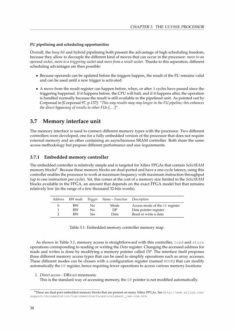
CHAPTER 3. THE ULYSSE PROCESSOR

FU pipelining and scheduling opportunities

Overall, the busy bit and hybrid pipelining both present the advantage of high scheduling freedom,because they allow to decouple the different kind of moves that can occur in the processor: move to anoperand socket, move to a triggering socket and move from a result socket. Thanks to this separation, differentscheduling advantages are then possible:

• Because operands can be updated before the triggers happen, the result of the FU remains validand can be used until a new trigger is activated.

• A move from the result register can happen before, when, or after λ cycles have passed since thetriggering happened. If it happens before, the CPU will halt, and if it happens after, the operationis handled normally because the result is still available in the pipelined unit. As pointed out byCorporaal in [Corporaal 97, p.137]: “This way results may stay longer in the FU pipeline; this enhancesthe direct bypassing of results to other FUs [. . . ]”.

3.7 Memory interface unit

The memory interface is used to connect different memory types with the processor. Two differentcontrollers were developed, one for a fully embedded version of the processor that does not requireexternal memory and an other containing an asynchronous SRAM controller. Both share the sameaccess methodology but propose different performance and size requirements.

3.7.1 Embedded memory controller

The embedded controller is relatively simple and is targeted for Xilinx FPGAs that contain SelectRAMmemory blocks8. Because these memory blocks are dual-ported and have a one-cycle latency, using thiscontroller enables the processor to work at maximum frequency with maximum instruction throughput(up to one instruction per cycle). Yet, this comes at the cost of a memory size limited to the SelectRAMblocks available in the FPGA, an amount that depends on the exact FPGA model but that remainsrelatively low (in the range of a few thousand 32-bits words).

Address RW mode Trigger Name – Function Description

0 RW No Mode Access mode of the DP register1 RW No DP Data pointer register2 RW Yes Data Read or write a data

Table 3.1: Embedded memory controller memory map.

As shown in Table 3.1, memory access is straightforward with this controller, load and storeoperations corresponding to reading or writing the Data register. Changing the accessed address forreads and writes is done by modifying a memory pointer called DP. The interface itself proposesthree different memory access types that can be used to simplify operations such as array accesses.These different modes can be chosen with a configuration register (named MODE) that can modifyautomatically the DP register, hence requiring fewer operations to access various memory locations:

1. Direct access - DREAD mnemonicThis is the standard way of accessing memory, the DP pointer is not modified automatically.

8These are dual-port embedded memory blocks that are present on many Xilinx FPGAs. See http://www.xilinx.com/support/documentation/topicmeminterfacestorelement_ram-rom.htm

38

3.7. MEMORY INTERFACE UNIT

2. Auto-incremented mode - AUTOINC mnemonicEvery read or write operation in memory is followed by an automatic increment of the DP pointer.This mode can be used to read consecutive elements in an array.

3. Stack mode - STACK mnemonicAfter each read operation, the DP pointer is decremented (operation pop) and every writeoperation triggers the increment of the DP (operation push). With this mode a stack segmentcan be easily generated, which is useful for implementing function calls, for example. The stackrealized is of “drum” type, which means that when one of the boundaries of the memory isreached, the memory access is wrapped to the other end. For instance, if the pointer equals to 0and a pop operation is realized, the pointer will be updated with the highest address. Note thatthe position of the pointer is updated after the operation itself (post auto-modified scheme).

3.7.2 Asynchronous SRAM FU and controller

Fetch addressFetch data

Bus interface

Low-levelSRAM Controller

Statemachine

DataAddress[17...0]Data[15...0]nOE

nCS0nCS1

nWE

Interconnection bus

Address[17...0]

Clk

Clk4x

Data[31...0]

Address

SP1 SP2

+

Statemachine

Ext. addressExt. data

Dat

a re

ad[3

1...0

]

Stack o�setselection

Address sourceselection R

ead/

Writ

e op

Ext. REQ

Figure 3.7: The SRAM controller FU schematic.

This memory controller (Figure 3.7) is more complex and enables access to asynchronous SRAMmemory chips. It provides three main functionalities:

1. It provides instructions to the fetch unit. Read requests issued by the fetch unit are handled by adedicated bus between the fetch unit and the controller.

2. It provides access to the memory from the program application: because no dedicated instructionsexist to access memory in the architecture, load and store operations are “emulated” by thereading and writing of an address value at particular locations. These accesses modify a registercalled DATA as follows: when a load operation occurs, the resulting value can be read in thisregister; a store operation requires to write the value to be stored into memory to this registerfirst and then trigger the store operation by writing the address to the corresponding triggerregister.

Two registers, SP1 and SP2 can be used to automatically compute addresses with offset values,which can be handy and save some execution cycles for example in function calls.

39

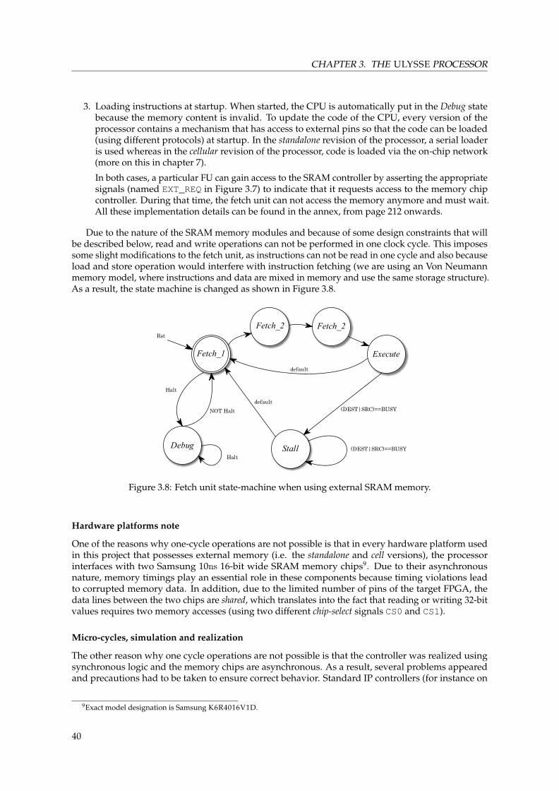
CHAPTER 3. THE ULYSSE PROCESSOR

3. Loading instructions at startup. When started, the CPU is automatically put in the Debug statebecause the memory content is invalid. To update the code of the CPU, every version of theprocessor contains a mechanism that has access to external pins so that the code can be loaded(using different protocols) at startup. In the standalone revision of the processor, a serial loaderis used whereas in the cellular revision of the processor, code is loaded via the on-chip network(more on this in chapter 7).

In both cases, a particular FU can gain access to the SRAM controller by asserting the appropriatesignals (named EXT_REQ in Figure 3.7) to indicate that it requests access to the memory chipcontroller. During that time, the fetch unit can not access the memory anymore and must wait.All these implementation details can be found in the annex, from page 212 onwards.

Due to the nature of the SRAM memory modules and because of some design constraints that willbe described below, read and write operations can not be performed in one clock cycle. This imposessome slight modifications to the fetch unit, as instructions can not be read in one cycle and also becauseload and store operation would interfere with instruction fetching (we are using an Von Neumannmemory model, where instructions and data are mixed in memory and use the same storage structure).As a result, the state machine is changed as shown in Figure 3.8.

Debug Stall

ExecuteFetch_1

Halt

default

(DEST|SRC)==BUSY

defaultNOT Halt

Halt

(DEST|SRC)==BUSY

RstFetch_2 Fetch_2

Figure 3.8: Fetch unit state-machine when using external SRAM memory.

Hardware platforms note

One of the reasons why one-cycle operations are not possible is that in every hardware platform usedin this project that possesses external memory (i.e. the standalone and cell versions), the processorinterfaces with two Samsung 10ns 16-bit wide SRAM memory chips9. Due to their asynchronousnature, memory timings play an essential role in these components because timing violations leadto corrupted memory data. In addition, due to the limited number of pins of the target FPGA, thedata lines between the two chips are shared, which translates into the fact that reading or writing 32-bitvalues requires two memory accesses (using two different chip-select signals CS0 and CS1).

Micro-cycles, simulation and realization

The other reason why one cycle operations are not possible is that the controller was realized usingsynchronous logic and the memory chips are asynchronous. As a result, several problems appearedand precautions had to be taken to ensure correct behavior. Standard IP controllers (for instance on

9Exact model designation is Samsung K6R4016V1D.

40

3.7. MEMORY INTERFACE UNIT

0 1

8061 0002

idle read1 read2 read3 read4 read5 read6 read7 read8 read9 read10 read11 idle

idle fetch1 fetch2 fetch3 idle

execute fetch1 fetch2 fetch3 execute

20ns 40ns 60ns

clkclk 4x

SRAM AddressSRAM Data

nOEnWEnCS0nCS1

SRAM ctrl stateMemory FU state

Fetch unit state

(a) Fetch and execute

0 70 61 0 72 62

0000 0AFE 8063 0048 0000 0AFA

idle w1 w2 w3 w4 w5 w6 w7 idle r1 r2 r3 r4 r5 r6 r7 r8 r9 r10 r11 r1 r2 r3 r4 r5 r6 r7 r8 r9 r10 r11 idle r1

idle prestore_operation store_operation fetch1 fetch2 fetch3 idle load1 load2 load3 fetch1

execute stall fetch1 fetch2 fetch3 execute stall fetch1

40ns 80ns 120ns 160ns 200ns

0

0AF

w1 w2 w3 w4 w5 w6 w7 idle r1 r2 r3 r4 r5 r6 r7 r8 r9 r10 r11 r1 r2 r3 r4 r5 r6 r7 r8 r9 r10 r11 idle r1idle

store_operation

execute

clkclk 4x

SRAM AddressSRAM Data

nOEnWEnCS0nCS1

SRAM ctrl stateMemory FU state

Fetch unit state

(b) Effects of a load after store

Figure 3.9: SRAM controller timings.

OpenCores10) normally require four clock cycles per read and write operation. However, using such acomponent would have required eight clock cycles per memory read, which would have hinderedperformance too much. To avoid this situation, we decided to optimize access as much as possible byimplementing our own controller.

Namely, we developed a controller using a separate clock running four times faster than the CPUclock, which was used to create micro-cycles inside the normal cycle period. Thus, using a clockfrequency of 50 MHz as an input, the fast clock generates four 5ns long cycles for every cycle. The fastclock drives a state machine that is used to ensure that all setup and hold constraints of the memoryare met in every possible case.

We had to use a very precise timing simulation model of the memory chips (with adequate setupand hold time checks) to ensure correct behavior. In addition, an unexpected problem that aroseduring the development of this component was that the different timing constraints also had to bestill valid outside the FPGA so that the memory chips could work. In fact, because of the routing andplacement delays inside the FPGA, signals generated during the same clock edge could present a fewnano-seconds of difference when measured at the FPGA pins.

To ensure correct behavior even in this case, synthesis constraints had to be added. To validate the

10http://www.opencores.org

41

CHAPTER 3. THE ULYSSE PROCESSOR

model on the actual hardware, the complete simulation model also includes place and route routingdelays to reflect as much as possible the real situation.

Figure 3.9 shows both a standard instruction fetch (3.9a) taking 3 cycles and a more interestingwaveform (3.9b) in which a load operation (3 cycles) is performed after a write operation (2 cycles),showing all the accesses of the controller. One can note that because memory load and store operationstake more than one cycle, the fetch unit should be prevented from reading the next instruction while amemory access operation is in progress. This is done using the busy bit mechanism.

Memory map

Address RW mode Trigger Name – Function Description

0 RW No SP1 Stack pointer number 11 RW No SP2 Stack pointer number 22 RW No Data Memory data register3 W Yes Load absolute Data←Memory(Address)4 W Yes Store absolute Memory(Address)← Data5 W Yes Load with offset 1 Data←Mem(Address + SP1)6 W Yes Load with offset 2 Data←Mem(Address + SP2)7 W Yes Store with offset 1 Mem(Address + SP1)← Data8 W Yes Store with offset 2 Mem(Address + SP2)← Data

Table 3.2: SRAM FU Interface.

To close the discussion regarding this functional unit, we present in Table 3.2 a high-level perspectiveof the functional unit showing how the unit is seen from a programmer’s perspective.

3.8 ULYSSE functional units

As shown in Figure 3.10, several functional units were developed as part of this work to accommodatethe various needs of the different versions of the ULYSSE processor. We will not detail them here butthe annex contains (see section A.2, p. 206) a description of the interface of these various operatorsas well as more practical information related to their operation. They can be classified into four maincategories (see Table 3.3):

1. ArithmeticThe first category contains arithmetic operators, i.e. FUs used to compute mathematical and logicalfunctions.

2. InterfaceThe second category contains units used to interface ULYSSE with the outside world.

3. GeneralThe third category is composed of units used in general operation of the ULYSSE processor or asinternal peripherals.

4. DebugThe last category contains functional units that are used for debugging purposes, by providingsimulation or debugging mechanisms.

In the remaining of this section, we will briefly focus on some operators that represent a stretch tothe TTA philosophy or that present some interest from a theoretical standpoint.

42

3.8. ULYSSE FUNCTIONAL UNITS

UlysseGeneral

Debug

Interface

Arith

Utilities

DCM

Register �le

TimerFetch

SRAM unit

Embedded memory

AssertionDebugger

DMA

GPIODisplay interface

Shift

ALUDivider

Multiplier

Concatenation

Comparison

Serial code receiver Mercury interface

Parallel shifter

Serial shifter

IP Divider

SRAM Controller

Functional unit

VHDL component

Figure 3.10: ULYSSE functional units hierarchy.

Name Latency λ Description

ALU 2 Common arithmetic/logic operations: +, −, ∨, ∧, ⊕, ¬, ×. See 3.8.3Shift sequential Vara Sequential version of SHL, SHR, SHRA, SHR, ROTR, ROTLShift parallel 2 Parallel version of SHL, SHR, SHRA, SHR, (ROTR, ROTL optional)Concatenation 2 To concatenate numbers. See 3.8.1Divider 43 To compute a/b and a mod bComparison 2 Allows to do various comparisons between two numbers. Also determines if

a number is positive, negative or null. See 3.8.2

GPIO 2 Simple FU to access the external input and output pins of the circuitCode receiver N/A Can be used to access the SRAM memory of the processor from the outside.

Used to upload the code when the processor is used in standalone modeMercury unit N/A Used in the cellular processor configuration as a high-speed network interface

to a routing system. It will be detailed in section 8.4.1Display interface 2 Used in the cellular processor configuration to interface with a LED display. It

will be detailed in section 8.4.2

Register file 2 Contains up to 32 general purpose registersTimer 2 A resettable timer that provides microsecond resolution to measure timeFetch unit N/A Fetches instructions and executes them. See section 3.6SRAM interf. 2 An interface to asynchronous SRAM memory chips. Provides LOAD and

STORE operations. See 3.7Embedded interf. 2 An interface to the Xilinx SelectRAM dual-ported memory blocks for LOAD

and STORE operations. Used only in the VLIW version of the processor

Assertion unit 2 Generates simulation exceptions and debug messages. See 5.1In-circuit debug. N/A In conjunction with the fetch unit, allows to pause and resume processor

execution. See section 5.3

aDepends on the number of shift operation performed.

Table 3.3: Arithmetic FUs available for the ULYSSE processor.

43

CHAPTER 3. THE ULYSSE PROCESSOR

3.8.1 Concatenation unit

As described in the instruction encoding (section 3.4.2), immediate values are stored in the instructionas 16-bit values.

If a bigger range is required, it is of course possible to compute bigger values with masks and shiftoperations. However, since 32-bits immediate values can be relatively common (and also becauseULYSSE is a full-fledged 32 bit processor), we implemented an unit whose purpose is to realize theconcatenation of values.

The unit is really simple as it contains only two inputs (A and B) and one output (R). It realizesthe following mathematical operation, which is trivial to implement in hardware (consisting of onlywires): R = (A� 16) ∨B.

3.8.2 Conditional instructions (condition unit)

Address RW mode Trigger Name Description

0 RW Yes OpA Operand A1 RW No OpB Operand B2 RW No OPcode Selects the operation performed3 R No Result Depending on OPCode: A < 0, A > 0,

A = 0, A 6= 0, A > B, A ≥ B, A < B,A ≤ B, A = B, A 6= B

Table 3.4: Condition functional unit.

The interest of this functional unit resides in the fact it is normally used to compute conditions forjump operations. In fact, the fetch unit can generate two different kinds of jump operations: eitherimmediate or conditional immediate. In the first case, the jump is always taken and in the second it istaken if and only if the condition register of the fetch unit is equal to 1.

Even if the condition register can be updated by any FU, the condition unit provides severalmethods to “emulate” standard jump conditions, as summarized in its memory map, shown in Table3.4. It can be remarked that we are using a different mapping mechanism for this operator in the sensewe are using an OPcode register that selects among the different operations realized, which all have alatency λ = 2.

This mechanism was chosen due to the large number of operations this FU can perform, which isin fact larger than the number of registers per FU that the VLIW version can address11.

3.8.3 Arithmetic and logic functional (ALU) unit

As we mentioned earlier, most ULYSSE implementations do not implement parallel displacements inthe form of VLIW instructions. Because of this, it becomes possible to regroup multiple arithmeticand logic units together since any scheduling advantage offered by separated FU is lost. Moreover,this grouping also allows to reduce the cost of multiple bus interfaces, which is positive even if businterfaces in themselves are not so costly in terms of hardware.

The ALU FU, for example, regroups many of the mathematical operations that are normally usedin a processor. Its memory map is shown in Table 3.5. Every operation has a latency of λ = 2 and thefunctional unit also presents the advantage that every one of its operations is done in parallel whenthe functional unit is triggered. The results of the different operations can then be read at differentlocations. This means that only one displacement is required to do every possible ALU operation,which in turn enables interesting scheduling opportunities because the results of all these operationscan be retrieved directly.

11Because the internal addressing space in this version is smaller than the others, only 3 bits are devoted to page addresses,which restricts the maximum number of registers per FU to 8.

44

3.9. HARDWARE PERFORMANCE EVALUATION

Address RW mode Trigger Name Description

0 RW No OpA Operand A1 RW Yes OpB Operand B2 R No Add A+B3 R No Substract A−B4 R No OR A ∨B5 R No AND A ∧B6 R No NOT ¬B7 R No XOR A⊕B8 R No Multiplylow (A ·B)[31...0]

9 R No Multiplyhigh (A ·B)[63...32]

Table 3.5: ALU functional unit.

3.9 Hardware performance evaluation

In this section, we will examine the performance of the ULYSSE processor from a hardware perspective,i.e. focusing on hardware requirements such as size estimations per FU, achievable frequencies. . . . Thisanalysis will be completed, in chapter 5 (section 5.5), after programming tools such as the compilerwill be introduced, by an extensive analysis of the processor including different software benchmarks.

Our discussion will be targeted on the cellular version of the processor because it is the mostcomplete and the most interesting in the context of this thesis.

3.9.1 Ulysse’s FU size and speed

Table 3.6 summarizes the hardware related information computed using the Xilinx ISE 10.1 tool suitealong with the Synplify Pro 9.0.1 logic synthesizer. The functional unit figures are estimates based onthe synthesis of the functional unit with its complete bus interface. The three last rows of the tablerepresent final CPU size and speed results based on a post-place-and-route analysis.

3.10 Possible further developments

Developing a processor from the ground up takes time and can be considered as an endless task, newoperators and increased performance being constant objectives. In its current state, the processorcould benefit from the implementation of caching techniques so that it could reduce its CPI, notablywhen using external memory. Of course, more performance could also be attained by overcomingthe weaknesses related to the VLIW revision. Finally, designing a FU to access (or bridge) industry-standard buses such as ARM, AMBA [Flynn 97], or the IBM CoreConnect series (OPB/PLB)12 wouldalso allow various existing IP modules to be used, be they free or commercial.

Besides implementation-related improvements, one research opportunity that could be interestingto follow would be to push the idea of pluggable FUs further by extending the architecture so thatit could support dynamic reconfigurability. Consisting of changing the configuration of parts of thereconfigurable hardware on line, this technique could enable to use free zones that could implementnew operators suitable for different algorithms depending on the executed program. While similarapproaches have been proposed in the past (for example [Epalza 04, Jain 04]), the Move paradigmproposes useful features that other architectures lack.

12http://www.xilinx.com/support/documentation/ip_documentation/opb_v20.pdf

45

CHAPTER 3. THE ULYSSE PROCESSOR

Functional unit description LUT Register bits Max freq.

ALU without 32× 32 multiplier 493 418 > 200 MHzALU with 32× 32 multipliera 525 496 > 200 MHzParallel shifter, without rot ops 606 245 > 200 MHzParallel shifter, with rot ops 1005 486 > 200 MHzConcatenation 76 32 > 200 MHzRF (8 registers) 256 400 > 200 MHzSRAM memory 399 323 > 200 MHz

Condition unitb 254 272 172 MHzTimer 59 40 180 MHzFetch unit 252 121 132 MHzCode uploader 80 61 140 MHzDividerc > 452 > 762 > 50 MHz

Routing interfaced 111 85 100 MHzMercury receiver 299 190 157 MHz

Smalleste CPU 756 362 52 MHz

Usablef CPU 2562 1154 54 MHzFull CPU (after PR) 2975 1371 53 MHz

aUses 4 multiplier blocksbCritical path on the “=” operationcCould only provide lower bounds because IP module can not be fully estimated due to license restrictionsdUses 1 BRAM moduleeSupport FUs onlyf69% of Spartan3–XCS200 FPGA; no mult, no timer, no cat unit

Table 3.6: Size and speed of available ULYSSE functional units.

3.10.1 Permanent connections and meta-operators

We propose here a method that enables, by adding a certain number of buses, to increase ILP sothat more instructions are executed than instruction slots are present. Even if this technique was notimplemented due to time restrictions, we think its description could lead to an interesting increase ofperformance.

In fact, as we have already mentioned, a possible method to increase the performance of a processoris to increase ILP, something TTA enables thanks to VLIW instructions. However, this parallelism islimited by the number of slots per instruction. In case of repetitive operations, it might be interestingto specify that a displacement must be permanently done (at each instruction) until further notice.

As the operators implemented possess for the most part a relatively low latency and because itis simple to move data in series and in parallel, it might be interesting to introduce the concept ofmeta-operator.

To illustrate the concept, let us consider a standard DSP instruction such as the MACC (multiply-and-accumulate). Let us now imagine that this operation is not directly present as an FU but that we want touse it anyway: with one multiply and one add FU, the code corresponding to the MACC operation is thefollowing:

/∗ MACC operation equivalent∗/loop:

move multiplier_a_t, operand1;move multiplier_b, operand2;move adder_a_t, adder_result;move adder_b, multiplier_result;[...]

As the accumulation of results is done during the whole loop, the second displacement couldbe specified as permanent and done in parallel, reducing the size of the operation kernel. Figure3.11 represents the required configuration of an automatic MACC operator, which corresponds to the

46

3.10. POSSIBLE FURTHER DEVELOPMENTS

following code:

/∗ MACC operation with permanent connections∗/move_perm adder_a_t, adder_result;move adder_b, multiplier_result;

loop:move multiplier_a_t, operand1;move multiplier_b, operand2;[...]

Adder

Transport bus 1

Transport bus 0

Transport bus 2

Transport bus 3

Multiplier

Permanent connections

Temporary connections

Figure 3.11: MACC with permanent connections.

The concatenation of the multiply and add operations thanks to permanent connections is what wecall a meta-operator. Its latency is equal to the sum of the latencies of the pipelined functional units. Inthe general case:

λtot =n∑i=0

λi n being the number of operators in series (3.3)

Which yields

λtot ∈ O(n) (3.4)

The working frequency of the resulting system will depend in the worst case of the slowestfunctional unit. As in every operator the critical path traversal time δ is short because it lies betweentwo registers, the resulting pipeline can also work at a high frequency. More formally, we have that:

∀i, i 6= max⇒ δmax > δi max being the latency of the slowest operator (3.5)δtot = δmax ⇒ δtot ∈ O(1) (3.6)

Of course, the use of permanent connections requires supplementary communication buses. Fur-thermore, the assembler or the compiler must be able to take these permanent connections into accountto determine the existence of free transfer buses. In counterpart, processor parallelism is increased asmore displacements than slots can be realized.

Research in this direction could also try to examine automatic allocation and assignation of buses,notably by analyzing if an algorithm could determine an optimal transfer scheme, at the compiler levelfor example, between permanent or temporary moves.

47

CHAPTER 3. THE ULYSSE PROCESSOR

3.11 Conclusion

With the description of the ULYSSE processor from an hardware standpoint, we were able to demon-strate that the architecture suits our needs by providing various levels of flexibility, such as thepluggability of FUs or the pipelining opportunities with the busy bit mechanism, while remainingrelatively cost effective.

One of the main goals of the implementation was to validate the model and to show that it wasable to provide the user with enough flexibility to fulfill its task as a bio-inspired processor. Adding anew operator is simple and straightforward: by implementing the VHDL bus interface and specifyingthe number of accessible registers in the FU, the component is automatically added to the memorymap of the processor. Of course, this must be done before synthesis. Still, it is possible to define anad-hoc processor that can be specific for each application very easily.

The following example shows how this translates in the entity of the processor itself:

entity ulysse_cell isgeneric(

clk_frequency : positive := 50000000;alu_present : positive := 1;enable_multiplier : boolean := true;concat_present : positive := 1;rf_present : positive := 1;divider_present : positive := 0;shift_present : positive := 1;enable_rot_op : boolean := false ;has_timer_1 : boolean := true;has_timer_2 : boolean := true;mercury_interface_present : boolean := true;routing_interface_present : boolean := true;

) ;

With this interface, changing the presence or even the number of instances of a particular FU in animplementation is only a matter of changing the generic parameters of the processor.

In the next chapter, we will examine how the achieved hardware flexibility translates at thesoftware level and also how it can be leveraged to ease development of programs and also of the toolsthemselves.

48

Bibliography

[Corporaal 91] Henk Corporaal & Hans (J.M.) Mulder. MOVE: a framework for high-performanceprocessor design. In Supercomputing ’91: Proceedings of the 1991 ACM/IEEEconference on Supercomputing, pages 692–701, New York, USA, 1991. ACM.

[Corporaal 93] Henk Corporaal & Paul van der Arend. MOVE32INT, a sea of gates realization ofa high performance transport triggered architecture. Microprocessing and Micropro-gramming, vol. 38, pages 53–60, 1993.

[Corporaal 97] Henk Corporaal. Microprocessor Architectures: From VLIW to TTA. John Wiley &Sons, Inc., New York, USA, 1997.

[Epalza 04] Marc Epalza, Paolo Ienne & Daniel Mlynek. Dynamic reallocation of functional unitsin superscalar processors. In Proceedings of the 9th Asia-Pacific Computer SystemsArchitecture Conference, pages 185–198, Beijing, August 2004.

[Flynn 97] D. Flynn. AMBA: enabling reusable on-chip designs. IEEE Micro, vol. 17, no. 4, pages20–27, Jul/Aug 1997.

[Hoffmann 04] Ralph Hoffmann. Processeur à haut degré de parallélisme basé sur des composantessérielles. PhD thesis, École Polytechnique Fédérale de Lausanne, 2004.

[Hoogerbrugge 96] Jan Hoogerbrugge. Code generation for Transport Triggered Architectures. PhD thesis,Delft University of Technology, February 1996.

[Jain 04] Diviya Jain, Anshul Kumar, Laura Pozzi & Paolo Ienne. Automatically customisingVLIW architectures with coarse grained application-specific functional units. In Proceed-ings of the 8th International Workshop on Software and Compilers for EmbeddedSystems (SCOPES’04), pages 17–32, Amsterdam, September 2004.

[Lin 04] C.H. Lin, Y. Xie & W. Wolf. LZW-based Code Compression for VLIW EmbeddedSystems. In Proceedings of the conference on Design, automation and test inEurope (DATE’04), pages 76–81, 2004.

[Myers 81] Glenford J. Myers. Advances in Computer Architectures. Wiley-Interscience, 1981.

[Xie 01] Y. Xie, W. Wolf & H. Lekatsas. Code Compression for VLIW Processors. In Proceedingsof the 34th International Symposium on Microarchitecture (MICRO 01), pages66–75, 2001.

49

Chapter 4

Development tools

“Well, less is more, Lucrezia.”

ROBERT BROWNING, Andrea del Sarto

ONE OF THE dangers in designing complex hardware systems in an academic setting is that thecomplexity of the development, coupled with the difficulty to adequately test the hardware,

often monopolizes all the resources, to the expense of software support. TTA processors do escapethis rule, but their modularity enable the application of interesting techniques for their testing. Incounterpart, their programming in assembly language is more complex than traditional processorsbecause they do not directly provide the programmer the traditional abstractions he or she expects.

The subject of this chapter is to analyze how the latter issue can be tackled with different tech-niques such as macros and how modularity can be exploited to simplify the testing of the processors.This discussion will focus on the ULYSSE processor, but the underlying principles could be, in general,applied to any Move processor.

The second part of this chapter will focus on the peculiarities of Move programming and how theyinfluenced the development of an assembler for the processor. In section 4.2, we will analyze some ofthe difficulties encountered during the port of the GCC compiler for our processor.

4.1 The assembler

The ULYSSE assembler is a software tool that transforms assembly code into its executable binary form.In this section, we will show that the use of a single instruction, because of the narrow perspectiveoffered, limits the low-level programmability of such a processor. To overcome this limit, we willdevelop the notion of macros, an abstraction that offers a higher-level view of the processor whileconserving its basic operation.

Because it also constitutes an essential component of the software tool-chain for the ULYSSE pro-cessor, the assembler has to be carefully designed and a choice must be made among the differentimplementation options offered. In our case, we preferred to focus on the back-end of the tool (thecode generation) by using an existing Java grammar parser generator (explained in section 4.1.9) thatconsiderably simplifies the use of multiple passes during the assembly.

4.1.1 Assembly process

The different assembly phases (shown in Figure 4.1) through which the assembly source code mustbe processed are the following:

1. Lexical verificationDuring this first phase, the part of the assembler called the lexer makes sure that the input pro-gram is compatible with the language grammar. The comments are eliminated along with the

51

CHAPTER 4. DEVELOPMENT TOOLS

Lexer

Parser Treescanning

Assembly programs in

ASCII formatdef val_1, 12;move r0, #val_1;

Representation

Tokens list

VAR, LITERAL,MOVEOP, IDENTIFIER

Representation

Syntactic trees

Representation

Assembled code

00101001010100101001010010

Representation

Figure 4.1: Description of the various phases of assembly.

carriage returns, separators such as “;”, etc. After this phase, the program has been transformedin a set of tokens. This pass is also used to take care of variables declaration: each time a variableis encountered, it is stored in a hash table (the key being the name of the variable) that will beused later on to verify, for example, if a variable has been already declared.

2. Syntactic verificationDuring this phase, the assembler verifies that the program follows the language syntax andproduces the syntactic tree corresponding to the program. Depending on whether an instructioncontains an immediate value or not, two nodes are possible:

(a) Displacement address, immediateThe left child is the destination address and the right child is the immediate value. Thedestination address and the immediate values are stored in the children nodes.

(b) Displacement address, addressThe left child is the destination address and the right child is the source address. Theaddresses are stored in their respective nodes.

This parsing phase was implemented using the Visitor design pattern which was defined byGamma et al. in their seminal work on design patterns [Gamma 95], which presents program-ming practices that can be applied to several common programming problem. We also refer theinterested reader to [Palsberg 98], which gives a more specific overview of the Visitor pattern.

3. Code generationThis last phase generates the executable code of the processor. The generation is done by recur-sively parsing the nodes of the syntactic tree produced during the second phase. Label addressesare computed and variable declarations are checked.

A simple example

We will illustrate now how the phases of the assembly process are applied to a simple program:

def r0, (9, 0); // Declaration of the R0 register using its paginated addressdef v1, 25; // Declaration of an alias for the constant value 25move r0, #v1; // Displacement of the immediate value 25 to the register r0

52

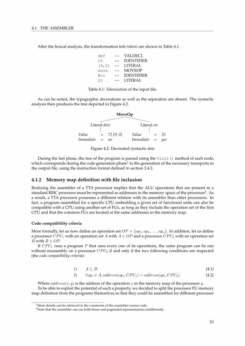
4.1. THE ASSEMBLER

After the lexical analysis, the transformation info tokens are shown in Table 4.1.

def 7→ VALDECLr0 7→ IDENTIFIER(9,0) 7→ LITERALmove 7→ MOVEOP#v1 7→ IDENTIFIER25 7→ LITERAL

Table 4.1: Tokenization of the input file.

As can be noted, the typographic decorations as well as the separators are absent. The syntacticanalysis then produces the tree depicted in Figure 4.2.

MoveOp``````

Literal dest

Value = 72 [9, 0]Immediate = no

Literal src

Value = 25Immediate = yes

Figure 4.2: Decorated syntactic tree

During the last phase, the tree of the program is parsed using the Visit() method of each node,which corresponds during the code generation phase1 to the generation of the necessary transports inthe output file, using the instruction format defined in section 3.4.2.

4.1.2 Memory map definition with file inclusion

Realizing the assembler of a TTA processor implies that the ALU operations that are present in astandard RISC processor must be represented as addresses in the memory space of the processor2. Asa result, a TTA processor possesses a different relation with its assembler than other processors. Infact, a program assembled for a specific CPU embedding a given set of functional units can also becompatible with a CPU using another set of FUs, as long as they include the operation set of the firstCPU and that the common FUs are located at the same addresses in the memory map.

Code compatibility criteria

More formally, let us now define an operation set OP = {op1, op2, . . . , opn}. In addition, let us definea processor CPU1 with an operation set A with A ∈ OP and a processor CPU2 with an operation setB with B ∈ OP .

If CPU1 runs a program P that uses every one of its operations, the same program can be runwithout reassembly on a processor CPU2 if and only if the two following conditions are respected(the code compatibility criteria):

1) A ⊆ B (4.1)2) ∀opi ∈ A, address(opi, CPU1) = address(opi, CPU2) (4.2)

Where address(x, y) is the address of the operation x in the memory map of the processor y.To be able to exploit the potential of such a property, we decided to split the processor FU memory

map definition from the programs themselves so that they could be assembled for different processor

1More details can be retrieved in the comments of the assembler source code.2Note that the assembler can use both linear and paginated representations indifferently.

53

CHAPTER 4. DEVELOPMENT TOOLS

versions without having to change the code itself. The code related to the execution of instructions isthus clearly separated from the hardware dependent source code.

4.1.3 Definition of new operators

The memory mapping mechanism is also interesting when new operators in the form of FUs haveto be added, because assembler support is direct: the operator memory map simply has to be addedto the memory map definition file and it can be then directly used. Modifying in a similar way anassembler for a RISC processor, for example, would require the assembler code to be modified andthen recompiled, at least when changing basic operations such as add. In TTA, as everything can beconsidered as a data displacement, even basic operations can be easily and rapidly changed.

One development that could be interesting to harvest the flexibility of the system would be toautomate the generation of the memory map that corresponds to the program to be executed. By de-termining the set of operators required to execute a given program, a minimal custom processor couldbe automatically generated along with its memory map (see notably on this subject [Hoffmann 04,chapter 19]). Thus, different processors would be easily generated for different programs, with theadvantage that only useful FUs would be present.

4.1.4 Macros and their influence on the definition of a meta-language

Because a n-operand, m result operation can be translated into n+m move operations [Corporaal 99],writing programs using only data transports is a very complex task, at least when realized by hand atthe assembly level. The very low level vision renders basic operations fastidious. Let us now considera small code snippet:

while(c != 0){c--;

}

A direct translation to non-optimized Move assembly, if we suppose variable c is stored in registerr0, gives:

loop:// Compute c−1 and put the result in r0move adder_a, r0;move adder_b_t, #-1;move r0, adder_r;

// Check if r0 == 0move cond_op, #zero;move cond_a_t, r0;move jump_condition, cond_result;

// If r0 != 0, jump to loopmove jabs_cond, #loop;

Even if not impossible, the above code takes time to write and is difficult to read. This can beexplained by the fact that, while seeing the program as displacements provides some advantagesfrom an hardware perspective, considering the program flow as only Move operations requires a nonnegligible amount of adaptation from the programmer.

To counter this situation, we added to the assembler the possibility to define macros, that is, ruleswhich transform a single statement into a sequence of instructions so that programming becomes lessweary. These macros can use an arbitrary number of parameters and calls can be present in their def-inition. Using macros creates distance from the architecture model and allows the creation of a morepractical meta-language that is based on displacements only but whose syntax is closer to traditionalassembly programming. Of course, this approach hides somewhat the fact that every operation con-sists of data displacements in the architecture, but the flexibility gained for the programmer is worth

54

4.1. THE ASSEMBLER

it, especially since the meta-language does not hinder the usage of a more low-level perspective if itis required.

begin:move jump_condition, #1;move jabs_cond, #after ; // Shall normally jump

move assert_line, #current_line;move assert_a_t, #1 || move assert_b, #2; // Hangs if here

after:move adder_b_t, #1;nop;move r0, adder_r;move cond_op, #zero || move cond_a_t, r0;nop;move jump_condition, cond_result;move jabs_cond, #dead_end;move assert_stop, #0;

dead_end:move assert_line, #current_line;move assert_a_t, #1 || move assert_b, #2; // Hangs if here

#include “ macros.inc ”

begin : jump after; // Shall normally jump error ; // Hangs if here

after : add #0 , #1 ; jz add_result, dead_end; exit ; // Everyhing ’ s ok

dead_end : error ;

With macros:Without macros:

Figure 4.3: Code sample written with and without macros.

Defining a meta-language proved very useful and effective, notably from a programmer’s perspec-tive. Figure 4.3 shows the same program implemented once with macros and once without.

It was thus possible to define function calls (with context saving on the stack) in a few lines ofcodes. In addition, the programmer can define additional complex macros that can be used for achiev-ing even higher-level operations (such as loops, complex tests, . . . ).

4.1.5 Code and data segments

The assembler offers the possibility to define various memory segments that refer to different memorylocations to store instructions and data, the first being defined by the .code keyword and the otherby the .data keyword. Even if different segments can be declared in the code by using the keywordsin multiple locations, the segments are gathered when generating the code so that the data segmentsimmediately follow the code segments (which start at address location 0).

To declare a data segment (i.e. variables stored in the memory), the .data keyword must beused. It can be optionally followed by the initial values of this code segment, declared by a label. Thefollowing example shows the process of declaring an array of 10 values with an initial content alongwith a 512-word zone with an initial value of 1 that can be accessed with the address vector_1:

.dataarray:.dw 16,12,14,14,18.dw 11,12,13,17,22

vector_1:.size 512 1

.code[...]

Listing 4.1: Declaration of a data segment.

55

CHAPTER 4. DEVELOPMENT TOOLS

4.1.6 Arithmetic expressions

In assembly, constants that depend on arithmetic expression are sometimes required. This is the casefor example when copying a memory zone. Let us now consider the following example, that uses theembedded memory controller, which proposes different addressing modes (see section 3.7.1):

move mem_op, #autoinc; // Use the auto−incremented addressing modemove dpa, #table_1; // Memory pointer = table_1move r0, #64; // Copy 64 elements

// While R0 6= 0, copy from a FIFO to table_1loop:

move memory_a, fifo; // Copy from a FIFO to table_1subr r0, r0, #1; // Decrement loop counterjnz r0, loop; // Loop counter = 0 ?

Listing 4.2: Non optimized array copy.

When arithmetic expressions are available in the assembler, the above code can be rewritten byusing the expected final value of DPA (computed with an arithmetic expression) as a test condition:

move mem_op, #autoinc; // Use the auto−incremented addressing modemove dpa, #table_1; // Memory pointer = table_1move r0, #(table_1 + 64); // Maximum value, using an arithmetic expression

// While DPA 6= R0, copy from a FIFO to table_1loop:

move memory_a, fifo; // Copy from a FIFO to table_1jneq dpa, r0, loop;

Listing 4.3: Optimized copy of an array.

With this code, the subtraction in the loop can be removed, which in this case translates to areduction of 3 move instructions from the loop (of the 8 initial instructions).

Arithmetic expressions can be used anywhere in the code and can be composed of an arbitrarynumber of parentheses. Labels can also be used in expressions, however only if they have alreadybeen declared when used3. This can be explained by the fact that expression resolution is done duringthe first pass of the assembly process and not during the parsing of the tree, for the sake of simplicity.However, by that time the position of every label is not yet determined. Even if this approach mightbe limited, it still proves useful.

The operators that can be used in the expression are the following4:

Op = {+,−, ∗, /,�,�,∨,∧,⊕}

With these expressions, masks can be realized as well as label relative operations, loop size compu-tations. . . , without having to use constant values in the code, which in any case is a bad programminghabit. Consequently, programs are more readable and more parameterizable, two characteristics thathelp reducing errors.

4.1.7 Immediate values and far jumps

In this section we will tackle the question of far jumps, that is, jumps in a program to an address thatis beyond the zone addressable by immediate values. It was stated in section 3.4.2 that immediatevalues use 16-bit values in the standalone and cellular versions whereas the VLIW version uses 9-bitimmediate values. This leads us to the definition of two kinds of immediate values: the short, whichcan be represented completely in an instruction, and the long, which exceeds the 16- or 9-bit limit. This

3If it is not the case, an error message is generated by the assembler.4The syntax is the one of the C language.

56

4.1. THE ASSEMBLER

differentiation is required whenever as the program is big enough that jumps beyond the immediatevalue limit are required. As it is not reasonable to ask the user to avoid jumping too far or to see if thegenerated code is correct, the assembler had to take these situations into account.

The solution is theoretically simple:

1. During the parsing of the tree, when a node whose value can not be represented by an imme-diate is discovered, multiple instructions have to be generated to separate this value in smallerpieces that fit the instructions. The immediate value so cut is thus displaced to the concatenationunit5 to form a bigger value. For example, completing the following operation:

move r0, #0xabcdef12;

requires to generate the following code to fit the instruction format:

move concat_0, #0xef12; // Low 16 bitsmove concat_1, #0xabcd; // High 16 bitsmove r0, concat_r; // Move result

2. The same solution has to be applied to labels, as they are also stored as immediate values.

The use of long immediate values implies that not one but many lines of code have to be generated.This implies that a further assembly pass is required in order to resolve labels correctly.

To assign addresses to labels, the labels are annotated with the current number of generated lineswhen encountered in the code. However, when a label is used in the code, one must consider thatif its address can not be reached by a short value, multiple instructions have to be generated. Thishas the consequence to invalidate all the labels situated after the line where the immediate had to beexpanded, because the number of lines of the program has been changed. To reflect the new situation,all the affected labels have to be incremented by the number of lines generated by the expansion.

An example makes this concept clearer:

label_1:jump far_label; // Jump to a yet unknown location

label_2: // label_2 value := 2move r1, add_r;

[...] // more than 0xFFFF lines for cell and standalone revisions , 0x1FF for the VLIW version

far_label:move r0, #1;jump label_2; // label_2 value used here is wrong (6= 2), as some lines will be added by the immediate

extension

Listing 4.4: Far jump example.

During the first pass, the jump far_label instruction will generate a node with an unknownvalue, which is normal. However, during the rest of the pass, the label label_2 will be declared aslocated at line 2, which is correct if far_label is not located outside the zone addressable by a shortimmediate, but at that moment we have no way to know it. As we continue parsing the tree, a jumpthat uses the concatenation unit will be done, which will imply that the label_2 and far_label need tobe changed, invalidating the program.

An elegant solution is provided by an additional assembly pass, for the following reasons:

1. The purpose of the Visitor design pattern is to realize different functionalities on a given tree.

5Note that we verify during assembly that such an unit is present in the processor by checking if the corresponding operandsare declared.

57

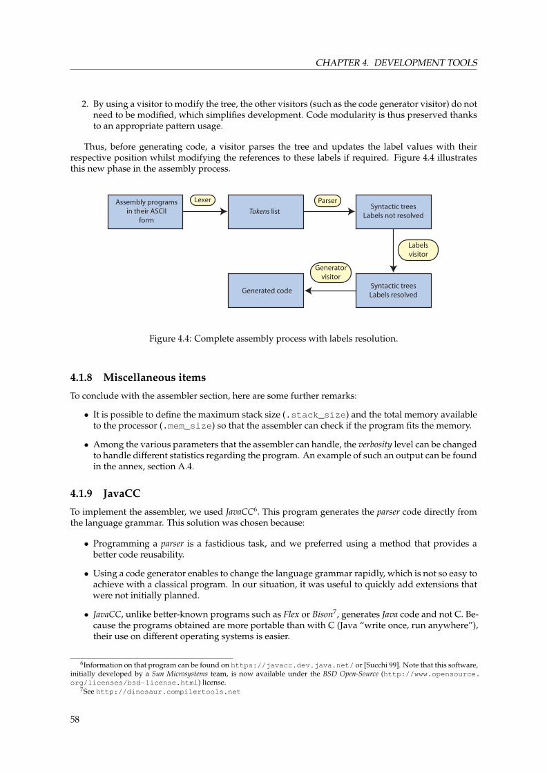
CHAPTER 4. DEVELOPMENT TOOLS

2. By using a visitor to modify the tree, the other visitors (such as the code generator visitor) do notneed to be modified, which simplifies development. Code modularity is thus preserved thanksto an appropriate pattern usage.

Thus, before generating code, a visitor parses the tree and updates the label values with theirrespective position whilst modifying the references to these labels if required. Figure 4.4 illustratesthis new phase in the assembly process.

Lexer Parser

Labelsvisitor

Assembly programsin their ASCII

formTokens list

Syntactic treesLabels resolved

Generatorvisitor

Syntactic treesLabels not resolved

Generated code

Figure 4.4: Complete assembly process with labels resolution.

4.1.8 Miscellaneous items

To conclude with the assembler section, here are some further remarks:

• It is possible to define the maximum stack size (.stack_size) and the total memory availableto the processor (.mem_size) so that the assembler can check if the program fits the memory.

• Among the various parameters that the assembler can handle, the verbosity level can be changedto handle different statistics regarding the program. An example of such an output can be foundin the annex, section A.4.

4.1.9 JavaCC

To implement the assembler, we used JavaCC6. This program generates the parser code directly fromthe language grammar. This solution was chosen because:

• Programming a parser is a fastidious task, and we preferred using a method that provides abetter code reusability.

• Using a code generator enables to change the language grammar rapidly, which is not so easy toachieve with a classical program. In our situation, it was useful to quickly add extensions thatwere not initially planned.

• JavaCC, unlike better-known programs such as Flex or Bison7, generates Java code and not C. Be-cause the programs obtained are more portable than with C (Java “write once, run anywhere”),their use on different operating systems is easier.

6Information on that program can be found on https://javacc.dev.java.net/ or [Succhi 99]. Note that this software,initially developed by a Sun Microsystems team, is now available under the BSD Open-Source (http://www.opensource.org/licenses/bsd-license.html) license.

7See http://dinosaur.compilertools.net

58

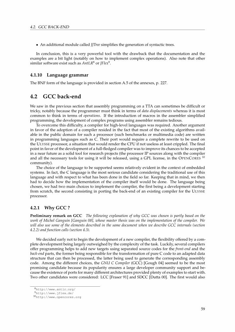
4.2. GCC BACK-END

• An additional module called JJTree simplifies the generation of syntactic trees.

In conclusion, this is a very powerful tool with the drawback that the documentation and theexamples are a bit light (notably on how to implement complex operations). Also note that othersimilar software exist such as AntLR8 or JFlex9.

4.1.10 Language grammar

The BNF form of the language is provided in section A.5 of the annexes, p. 227.

4.2 GCC back-end

We saw in the previous section that assembly programming on a TTA can sometimes be difficult ortricky, notably because the programmer must think in terms of data displacements whereas it is mostcommon to think in terms of operations. If the introduction of macros in the assembler simplifiedprogramming, the development of complex programs using assembler remains tedious.

To overcome this difficulty, a compiler for high-level languages was required. Another argumentin favor of the adoption of a compiler resided in the fact that most of the existing algorithms avail-able in the public domain for such a processor (such benchmarks or multimedia code) are writtenin programming languages such as C. Their port would require a complete rewrite to be used onthe ULYSSE processor, a situation that would render the CPU if not useless at least crippled. The finalpoint in favor of the development of a full-fledged compiler was to improve its chances to be acceptedin a near future as a solid tool for research projects (the processor IP sources along with the compilerand all the necessary tools for using it will be released, using a GPL license, in the OPENCORES 10

community).The choice of the language to be supported seems relatively evident in the context of embedded

systems. In fact, the C language is the most serious candidate considering the traditional use of thislanguage and with respect to what has been done in the field so far. Keeping that in mind, we thenhad to decide how the implementation of the compiler itself would be done. The language beingchosen, we had two main choices to implement the compiler, the first being a development startingfrom scratch, the second consisting in porting the back-end of an existing compiler for the ULYSSEprocessor.

4.2.1 Why GCC ?

Preliminary remark on GCC The following explanation of why GCC was chosen is partly based on thework of Michel Ganguin [Ganguin 08], whose master thesis was on the implementation of the compiler. Wewill also use some of the elements described in the same document when we describe GCC internals (section4.2.2) and function calls (section 4.3).

We decided early not to begin the development of a new compiler, the flexibility offered by a com-plete development being largely outweighed by the complexity of the task. Luckily, several compilersoffer programming helps to add new targets using separated source codes for the front-end and theback-end parts, the former being responsible for the transformation of pure C code to an adapted datastructure that can then be processed, the latter being used to generate the corresponding assemblycode. Among the different choices, the GNU C Compiler (GCC) [Gough 04] seemed to be the mostpromising candidate because its popularity ensures a large developer community support and be-cause the existence of ports for many different architectures provided plenty of examples to start with.Two other candidates were considered: LCC [Fraser 91] and SDCC [Dutta 00]. The first would also

8http://www.antlr.org/9http://www.jflex.de/

10http://www.opencores.org

59

CHAPTER 4. DEVELOPMENT TOOLS

have been appropriate but it was finally rejected due to a more limited documentation. The second,SDCC is aimed more at very small processors that work with less than 32 bits.

4.2.2 The GNU C Compiler – GCC

We followed the incremental approach of writing a back-end described by [Deshpande 07] but also inthe “Workshop on GCC internals”11. We will not go into too much detail here because writing a compilermainly consists of implementation-related issues. However, a complete “walkthrough” describing thewhole process can be found in Michel Ganguin’s master thesis report [Ganguin 08].

4.2.3 GCC components

GCC is more than “just” a compiler as it gathers together a preprocessor, an assembler program, astandard library for linking and, obviously the compiler itself. When GCC is called in a standard way,as in:

gcc [args] cfile.c -o program

In reality, four programs are used to generate the final binary executable code:

cpp -I/stdheaders [cpp specific args] cfile.c -o tmp.icc1 [cc1 specific args] tmp.i -o tmp.sas [as specific args] tmp.s -o tmp.old [ld specific args] -L/stdlibs -lc -lgcc tmp.o -o program

• cpp, the C preprocessor, handles preprocessor directives, such as includes and macro expan-sions. Some of the GCC arguments are passed to cpp, such as the -D flag, to define a macro12.Some target-specific macros are included, i.e. in this port the MOVE macro is defined (usable forexample to produce ULYSSE-specific code with #ifdef MOVE). cpp’s output is a C programwith macros resolved, comments removed, etc. It is part of GCC.

• cc1, the compiler, contains the whole compiler, front-end, “middle-end” and back-end. It pro-duces textual assembler code. Obviously, cc1 is part of GCC.

• as, the assembler program, produces binary code. It is not part of GCC but is a script that callthe real assembler program of the processor or may be a symbolic link to it.

• ld, the linker, brings together several assembled programs and allows the inclusion of libraries.

As we already have created the assembler program, we focused our attention on the cc1 part. Wedid not develop a linker, which means that the input, after preprocessing, has to be one single file(which can be achieved by adequate programming techniques).

4.2.4 The compilation process

When we consider the whole compilation process (Figure 4.5), GCC makes use of three intermediatelanguages:

• Starting from the source language, a front-end transforms the source code (e.g. C) into GENERIC,a high-level tree-based language in which some source-language specifics may remain.

• The second language is GIMPLE, a low-level tree-based language, more restrictive than GENERIC,but still source-language and target machine independent. GCC can perform several optimiza-tions directly on the GIMPLE form of the program (see 4.3.2).

11More details, presentation slides and code samples are available on http://www.cse.iitb.ac.in/~uday/gcc-workshop

12Note that C macros are different from assembly macros and are handled by the preprocessor in this case.

60

4.3. HANDLING FUNCTION CALLS

Parse

Gimplify SSAtransform

Sourcecode

High-level tree

GENERIC language

Representation

Low-level tree

Representation

GIMPLE language

SSA Tree

Representation

Gimpleto RTL

OptimizeRTL

RTL

Representation

List language

Optimized RTL

Representation

List language

Codegeneration

Assemblyform

Representationdef val_1, 12;move r0, #val_1;move adder_a, #1;

Platform independent

Platform dependent

RepresentationHigh-level language

C / C++ / ADA ...

Figure 4.5: The compilation phases.

• The third language is RTL, which consists in a stream of instructions that are transformed, inthe last pass of GCC, directly into assembler.

Writing a back-end is a twofold process. Firstly, the underlying mechanisms of the machine de-scription file, i.e. how instructions and constraints (number of registers, read–write access to register,memory layout, . . . ) are defined, must be understood. Secondly, the code generation process has tobe performed correctly.

In our opinion, the way the instructions are described within GCC is quite effective as it collectstogether different components, used at different locations in GCC’s source code, to minimize coderedundancy and to maintain a good overview of the processor. The GIMPLE to RTL translation isalso very well done: once the register constraints are correctly written, translation is transparent. Asa result, this first phase of the compilation is relatively straightforward.

The next phase, which works on the RTL representation, is more complex as new instructions areintroduced to match the constraints of the architecture. This representation starts with an unlimitednumber of registers. Several optimization passes that could not be done earlier can then be performed(see 4.3.2). Finally, register allocation is done, spilling to memory when required.

After this phase, the assembler code can be generated, based on the optimized RTL representation.

4.3 Handling function calls

In this section, we will explain how the functions are called with GCC. As function calls do not dependonly from the hardware, several implementation alternatives can be chosen. We have decided tostructure memory as depicted in Figure 4.6, with the code and data segments located at address 0 andthe stack growing downwards from the end of the memory.

ULYSSE does not provide a specific method to call functions, in the sense that calls are handled as“normal” jumps. For this reason, a prologue and an epilogue must be added to jumps to make them

61

CHAPTER 4. DEVELOPMENT TOOLS

Text segment (.data)

Code segment (.code)

Code limit

Stack segment

0x00000

0x3FFFF

Figure 4.6: Memory organization as seen by the compiler.

behave like functions calls. The major difference between jumps and calls is that the latter supposethat the control flow is resumed at the end of the call.

4.3.1 Saving state

To achieve this, we have at our disposal a specific register (RET) in which the caller can save the returnaddress before performing the call. From the callee’s perspective, there is only need to jump to thisaddress at function’s return.

Another piece of data that need to be saved are the arguments passed to a function and the returnvalue (in GCC, the latter can be considered as an additional argument). Therefore, for a non-voidfunction, the return value becomes the first argument and every nth argument is considered (n+1)th,as shown here:

// Function definitions can be considered asint foo(int a); -> void foo(int *retval, int a);

// Function calls are transformed to (not ANSI C, but correct in GNU C)int res = foo(43); -> int res = {int retval;

foo(&retval, 43);retval;}

All the function arguments are passed on the stack, in the order they are declared.In short, most of the work is done by the caller (saving the return address and the arguments,

changing the stack pointer) and it cannot leave values in registers across a call, as no register can beconsidered safe13. For the callee, all arguments are put on the stack and the return address is placedin the appropriate register.

4.3.2 GCC optimizations

One of the advantages of using a well-supported compiler such as GCC is that many optimizationsare directly available. Notably, GCC provides optimizations at different language levels, as we willnow examine.

13Which means that to hold a value over a call, it must be stored into memory before the call.

62

4.3. HANDLING FUNCTION CALLS

GIMPLE-level optimizations

In this language several optimizations are performed (see [Stallman 07, section 8.4]). These optimiza-tions are often called the “middle-end” of GCC, for they are source-language and target-architectureindependent. These optimizations include techniques such as:

• inlining, which consists in replacing the call to a function with its body;

• constant propagation, which consists in replacing constants or variables that are never modifiedby immediate values so no memory operation has to be performed;

• transformation into static single assignment (SSA) form, to simplify many aspects of code analysis.

RTL-level optimizations and operations

RTL is a language inspired by the Lisp list and the first form of RTL produced from GIMPLE uses anunlimited number of registers. After a second transformation, each RTL instruction corresponds to anassembler instruction (it is said to be in “strict RTL” form). Several optimization passes (mandatory oroptional, and which could not be done earlier in GIMPLE) are done on this language (see [Stallman 07,section 8.5]). Some of these are listed here:

• Control flow graph cleanupExamples are dead code elimination that removes unreachable code, jump simplification (totransform double jumps into single ones), etc.

• Common subexpression eliminationTo compute only once a common subexpression found in several different expressions.

• Liveness analysisLocates the first and last use of variables so determine the liveness of a variable. If the livenessof two variables overlaps, two different registers are needed to store them, but only one whenthey do not overlap. This analysis is useful, as in the former example, for register allocation butalso to locate unused variables.

• Instruction schedulingWhen there are different latencies for operations, instead of waiting for the end of a “long”operation, it is sometimes possible to execute further instructions. This implies that the programis executed out-of-order.

• Register allocationFinds the best available register candidate and, if there is none, uses a stack slot on memory. Theframe pointer can be eliminated in this pass, by computing its offset from the stack pointer. Thiselimination is mandatory for the ULYSSE processor, because of the limited number of registersthat can be used to directly access memory with an offset (see section 3.7, page 38).

• Final passGenerates the assembler code by translating each strict RTL instruction into its equivalent as-sembler form.

4.3.3 ULYSSE peculiarities for GCC

For some aspects of the compilation, the non-conventional nature of ULYSSE presented difficultiesduring the port of GCC for the architecture. Even if the purpose of this chapter is not to provide adetailed description of the structure of the GCC back-end and of the required implementation changesthat were undertaken to tailor it for ULYSSE, some aspects of its development are worth mentioningto illustrate the difficulties introduced by the use of non-conventional processors.

In fact, because GCC was initially designed for standard RISC/CISC processors in which opera-tions are not simple displacements, it was necessary to tell the compiler that moves into the trigger

63

CHAPTER 4. DEVELOPMENT TOOLS

registers had to be seen as the operations themselves. Because of the special semantics of the moveoperation, we had to inform GCC that some registers trigger operations, i.e. that a displacement tothese registers should not be considered as moves but as the operations themselves. If a read opera-tion of a register triggers an operation, it is also necessary to tell the compiler that the correspondingoperation has a double effect (this is not implemented in our code because all our trigger registers areread-only, see section 3.2.2 page 29.

Moreover, further problems were caused by the fact that some registers are read-only, such as theregisters holding results of operations. For GCC, every register is expected to be fully accessible whenperforming some of the optimization passes. Furthermore, due to the number of constraints on eachregister (readable or not, etc.) in the processor, GCC has sometimes trouble finding solutions forregister allocation.

Finally, we also had to face the fact that the GCC heritage can sometimes be problematic. Forinstance, the fact that ULYSSE uses a full 32-bit approach even for memory access (data words arenot aligned on bytes but on 32-bit words) was a source of multiple bugs during the developmentprocess, GCC being relatively lax on its definition of bytes, words and other sizes. . . . As a result,some constants that were supposed to automatically reflect different sizes had to be changed by handbecause they were implicitly supposing that accesses were done on 8-bit words.

4.3.4 Compiler optimizations specific to TTA

Although the implementation of a compiler for a TTA processor presented in this work remains sim-ple in the sense that a reliability objective was preferred over strict performance, optimizations specificto TTA can be undertaken. Even if these optimizations were not applied in the present GCC port, theyare worth mentioning because they provide interesting opportunities for improvement.

The most important contribution in the domain is the seminal work that was done by Hooger-brugge for his PhD thesis [Hoogerbrugge 96]. Notably, he proposed several kinds of optimizations.Let us now consider the following code14:

add r1, r2, r3; // r1 = r2 + r3;sub r4, r2, r5; // r4 = r2 − r5;store r4, r1; // mem[r4] = r1;

Listing 4.5: Code sample to optimize.

The direct translation of each of these n-operand, m-result operation results in the following n+mmove operations:

move add_a, r2; // first addition operandmove add_b_t, r3; // second addition operandmove r1, add_r; // move addition result to r1

move sub_a, r2; // first subtraction operandmove sub_b, r5; // second subtraction operandmove r4, sub_r; // move subtraction result to r4

move store_a, r4; // store address = r4move store_v_t, r1; // mem[store_address] = r1

Listing 4.6: Translation to move-only operations.

This straightforward translation offers several optimization possibilities, notably if multiple dis-placements are allowed. Before examining them, let us now define the concept of schedule in thecontext of TTA:

14This example is based on the explanation made in [Corporaal 99, p. 19–20] on the same subject and follows the samemethodology, although with a different notation.

64

4.3. HANDLING FUNCTION CALLS

Definition A schedule of a program is the temporal assignation of the corresponding data displace-ments among the different FUs of the processor using the existing move slots.

Using this definition, let us consider an example where four move slots are present in a processoralong with two separate arithmetic units, namely one for the add and one for the sub.

A possible schedule for the program 4.6 is the following :

Cycle Move slot 1 Move slot 2 Move slot 3 Move slot 41 r2→ add_a r3→ add_b_t r2→ sub_a r5→ sub_b2 add_r→ r1 sub_r→ r43 r4→ store_a r1→ store_v_t

If we consider now the possibilities to optimize this code, several opportunities arise, namely:

1. Data bypassingBecause the arithmetic results are present at the output of the two arithmetic units, they can bemoved directly to the memory unit without prior displacement to the r1 and the r4 registers.This allows to spare one cycle. The new scheduling is then:

Cycle Move slot 1 Move slot 2 Move slot 3 Move slot 41 r2→ add_a r3→ add_b_t r2→ sub_a r5→ sub_b2 sub_r→ store_a add_r→ store_v_t add_r→ r1 sub_r→ r4

2. Dead move eliminationIf the purpose of the r1 and r4 registers is only to store the intermediary results for the storeoperation, i.e. they are not used anywhere else before being rewritten, they can be consideredas dead code in the schedule and simply removed. In this example, this optimization does notimprove the timing of the schedule but its memory requirements. Thus, the resulting schedulebecomes:

Cycle Move slot 1 Move slot 2 Move slot 3 Move slot 41 r2→ add_a r3→ add_b_t r2→ sub_a r5→ sub_b2 sub_r→ store_a add_r→ store_v_t

3. Operand reuseIn some cases, operands can be reused if already present in a given FU, removing redundancy.For example, the following code:

add r1, r1, #1;add r2, r1, #1;

translates directly into the following move-only code:

move add_a, #1;move add_b_t, r1;move r1, add_r;move add_a, #1; // Uselessmove add_b_t, r1;move r2, add_r;

As the immediate value 1 is already present in the first operand of the adder, the marked instruc-tion is useless. This is of particular interest in single move bus implementations such as ULYSSEwhere one displacement corresponds directly to one clock cycle and can be used notably tospeed-up loops when adding offsets or increment values.

Even if it can not be considered as an optimization technique itself, TTA processors have the ad-vantage of increased freedom thanks to the fact that displacements and not operations have to bescheduled. Thus, because of the trigger mechanism, operands do not have to be moved at the sametime. Moreover, as many values can be stored directly into FUs without passing trough a central-ized register file, the scheduling constraints are lightened. Both phenomena allow more room forscheduling improvements.

65

CHAPTER 4. DEVELOPMENT TOOLS

4.4 Conclusion

During the development of the software tools to support our processor, we considered reliability ofthe software suite as the most important factor of development. Of course, efficiency is also importantbut we are intimately convinced that a working design is better than a fast but unreliable experience,especially in our context where even the hardware was developed from scratch. Thus, because soft-ware is easier to test than hardware, we put a lot of effort in obtaining robust tools that producedcorrect code.

The goal of a reliable and universal compiler was attained. We will see in the remainder of thiswork that it will be used to compile thousands of lines of C code with negligible problems. Porting acompiler such as GCC is an interesting challenge that requires a considerable amount of work and itshould come as no surprise that some problems and limits still persist:

• First, some optimizations are not always possible, a situation that limits the efficiency of thecode. In most “real”15 cases, optimizations have to be completely turned off, otherwise thecompiler crashes. Many problems have been identified as responsible for this. Unfortunately,solving them was impossible due to time reasons. However, the code produced when no op-timizations are used (which is done by compiling the programs with the -O0 flag) is correct.Thus, the compiler can fail but no incorrect code is ever produced.

• Secondly, neither software floating-point operations nor the C standard library have been en-tirely ported yet.

For further work on the tools themselves, the instruction scheduling should be improved and,since the TTA architecture allows to easily add new operations, the back-end should allow this flex-ibility too. Moreover, even though the hardware may resolve hazard dependencies automaticallythanks to the busy bit mechanism to ensure correct execution, the compiler should, when possible,take latencies of instructions into account to achieve best performance. Otherwise, FUs could unex-pectedly stall and reduce performance of the compiled code. On a more anecdotal level, a linker anda standard library should be also developed.

Except for these limitations, the assembler and the compiler are fully working and the resultsobtained so far are very encouraging: they open the way to the realization of high-complexity appli-cations on our bio-inspired substrate, as we will see in the next chapters.

15When the source code complexity is more than 10 lines

66

Bibliography

[Corporaal 99] Henk Corporaal. TTAs: missing the ILP complexity wall. Journal of Systems Archi-tecture, vol. 45, pages 949–973, 1999.

[Deshpande 07] Sameera Deshpande & Uday P. Khedker. Incremental Machine Description for GCC.Indian Institute of Technology, Bombay, 2007. http://www.cse.iitb.ac.in/~uday/soft-copies/incrementalMD.pdf.

[Dutta 00] Sandeep Dutta. Anatomy of a Compiler – A Retargetable ANSI-C Compiler. CircuitCellar Ink, no. 121, pages 30–35, Aug. 2000.

[Fraser 91] C. W. Fraser & D. R. Hanson. A Retargetable Compiler for ANSI C. Technical reportCS–TR–303–91, Princeton University, Princeton, N.J., 1991.

[Gamma 95] Erich Gamma, Richard Helm, Ralph Johnson & John Vlissides. Design Patterns:Elements of Reusable Object-Oriented Software. Addison-Wesley Professional Com-puting Series. Addison-Wesley Publishing Company, New York, USA, 1995.

[Ganguin 08] Michel Ganguin. A GCC Backend for the MOVE Architecture. Master’s thesis, ÉcolePolytechnique Fédérale de Lausanne (EPFL), 2008.

[Gough 04] Brian J. Gough & Richard M. Stallman. An Introduction to GCC. Network TheoryLtd., 2004.

[Hoffmann 04] Ralph Hoffmann. Processeur à haut degré de parallélisme basé sur des composantessérielles. PhD thesis, École Polytechnique Fédérale de Lausanne, 2004.

[Hoogerbrugge 96] Jan Hoogerbrugge. Code generation for Transport Triggered Architectures. PhD thesis,Delft University of Technology, February 1996.

[Palsberg 98] Jens Palsberg & C. Barry Jay. The Essence of the Visitor Pattern. In Proc. 22nd IEEEInt. Computer Software and Applications Conf., COMPSAC, pages 9–15, 1998.

[Stallman 07] Richard M. Stallman & The GCC Developer Community. GNU Compiler CollectionInternals. For GCC version 4.3.0. Free Software Foundation, 2007. http://gcc.gnu.org/onlinedocs/gcc.pdf.

[Succhi 99] Giancarlo Succhi & Raymond W. Wong. The Application of JavaCC to Develop aC/C++ Preprocessor. ACM SIGAPP Applied Computing Review, vol. 7, no. 3, 1999.

67

Chapter 5

Testing and performance evaluation

“Beware of bugs in the above code;I have only proved it correct, not tried it.”

DONALD KNUTH, 1977

THE DEVELOPMENT of a complete processor, especially with a design starting from scratch, requirescareful planning of the testing methodology to be used throughout the process. The ULYSSE

processor is no exception and we will discuss in this section the methodology we followed during thevarious phases of design. We will also demonstrate that TTA processors also present some advantageswhen it comes to testing, thanks to the common unified interface to which each functional unit mustadhere to.

Once the correct functioning of the processor is guaranteed to a certain extent, we will presentand discuss some experimental results in section 5.5 to evaluate the processor’s performance with aseries of benchmark programs. In this second part of the chapter, we will also evaluate how the codegenerated by our compiler compares, in terms of size and speed, to another 32-bit processor. Thiscomparison will serve as a confirmation that the implementation choices taken were reasonable, butalso that our bio-inspired approach does not hinder performance too much.

5.1 Testing methodology

To define how the processor was tested, some definitions are required.

5.1.1 Definitions

The testing methodology is closely based on the granularity of each component of the processor. Be-cause we used a bottom-up and very compartmentalized approach to build the processor, testing canfollow the same methodology. To determine the extent to which a component can be tested, we definethe following concepts:

1. Definition Two test vectors can be considered equivalent if and only if their application at theinputs of a component under test imply the same changes, in terms of internal state transitions,of the component. In other words, the internal state machine of the component follows the sametransitions, if any, for both test vectors.

To illustrate this concept of equivalence, let us now imagine the following situation, where thedesign of a 8-bit register must be tested.

69

CHAPTER 5. TESTING AND PERFORMANCE EVALUATION

Equivalence example

This component contains an 8-bit bus input for the data and three control inputs that representthe clock, reset and enable signals. The output of the device is also an 8-bit bus. To fully test thiscomponent, a normal test bench would need to check if all of the 211 different inputs combina-tions produce the correct output. However, if we can ensure that, due to the nature of systemunder test, the eight data bits are not used in the determination of the next state, their role isdifferent from that of the other inputs. As such, it is safe to consider equivalent the input vectorsthat only differ by their data bits. It is then possible to reduce the total number of test vectors to23. Of course, this reduction is only possible with a careful examination of the design that limitsits application to small designs, to avoid missing special cases.

2. Definition A testability metric ω is an estimate of the coverage of the total possible test cases bya given test bench. A testability ω = 1 signifies that every state and input combination of anhardware component can be checked and asserted by a test bench. Similarly, a testability ω = 0indicates that nothing can be tested about a component1.

The testability metric can be used, in conjunction with other criteria, to define testability classes,a concept that helps classifying hardware components in different categories that can then beused to pinpoint the origin of errors more easily. In our context, we consider the followingclasses:

(a) Class C1 - Fully testable componentsComponents for which every combination of inputs and states can be tested to guaranteefunctionality. To reduce the number of tests required, equivalent test vectors are used. Thetestability of these components is ω = 1.

(b) Class C2 - Functionally testable componentsComponents that can be tested to a point where it can be stated with a high level of confi-dence that the component’s functionality is verified thanks to a sufficient number of tests,even if an exhaustive test bench is not feasible. Particular attention should be paid to covercorner cases.

(c) Class C3 - Complex componentsComponents that require complex test benches, most of the time generated by programsbecause they imply a complex flow of operations. These components must be heavilyasserted (see next section) to cover all the branches of the flow.

(d) Class C4 - Irregular componentsThis category covers the components that are difficult to test because they possess a highnumber of inputs and internal states that can not be asserted easily. In addition to this, weput in this category every component driven by multiple clocks and/or that must synchro-nize across multiple clock domains.

(e) Class C5 - Black-box componentsThese components have the particularity that they only expose their input and outputssignals but their inside circuitry can not be accessed. The ω value for this kind of compo-nents is difficult, sometimes even impossible, to estimate because the input vectors that canbe applied to the inputs do not necessarily imply that every case is tested because of theinternal memory states.

Of course, ω is only an estimate and remains dependent on the designer’s experience. In andfor itself, the numerical value of the testability metric, besides the extremes, is not essential aslong as it allows to determine the degree of confidence the designer can have in the reliabilityof the component. Thus, during the design and test of the processor, the existence of testability

1Note that a testability of 0 is a degenerated case meaning that nothing can be tested about a component. This could happenfor example in the case of a component without outputs.

70

5.2. TESTING WITH ASSERTED SIMULATION

classes was primarily used to determine more quickly the order in which the components hadto be checked to find an error.

We will now introduce two methods we used to control the validity of the different classes.

5.2 Testing with asserted simulation

Whenever possible, we introduced assertions in the code to detect design failures. According to [Fos-ter 03, page 3], an assertion is

“[...] a statement about a design’s intended behavior (that is, a property), which mustbe verified. Unlike design code, an assertion statement does not contribute in any formto the element being designed. Its sole purpose is to ensure consistency between the de-signer’s intention, and what is created.”

Assertions should not be considered as components used to externally test components but ratherpart of the testing and development itself. During the development of the processor, three levels ofassertion were used, based on the language the assertion was done:

• VHDL levelAt the hardware description level, two different assertion languages were used:

– VHDL assert statements. This basic form of testing belongs directly to the VHDL lan-guage itself. It allows to check the consistency of simple assertions, such as in the followingexample:

assert (data_width - 1 = 31) report "IP Multiplier was generated with 32bits operands. You are using a different data width." severity error;

– Property Specification Language (PSL) statements. This language was recently developed[Foster 05, Eisner 06] to provide an assertion method both for verification and simulation[Boule 05]. It provides a lot more flexibility than standard VHDL asserts because time andstate relationships can be checked. A simple example such as

psl assert never (nCS0 = ’0’ and nCS1 = ’0’) report "Two nCS selected atthe same time";

would be more complex to realize with standard assertions, requiring intermediary signalsto achieve the same behavior. More complex example can also be considered:

−−Make sure that the address won’t change when fetching new datapsl assert always ((rst = ’0’ and fetch_mem_req = ’1’) -> next(prev(

fetch_mem_address) = fetch_mem_address))@(rising_edge(clk))report "Address not stable";

Both languages are supported by the simulator we are using (Mentor ModelSim SE PLUS version6.3f 2) and assertion failures are clearly indicated in the simulator. Depending on the severity ofthe assertion failure, the simulator can be stopped or simply textually indicate that an assertionfailed.

• Assembler levelThe goal of asserting assembly code is to guarantee that certain statements always hold. Situatedat a higher level than VHDL, assembler provides the first abstractions that enable behavioralchecking. In addition, assertions are also used in assembler as a method to report informationto the simulator or even to modify the simulation itself. These two cases are illustrated in thefollowing code:

2http://www.mentor.com

71

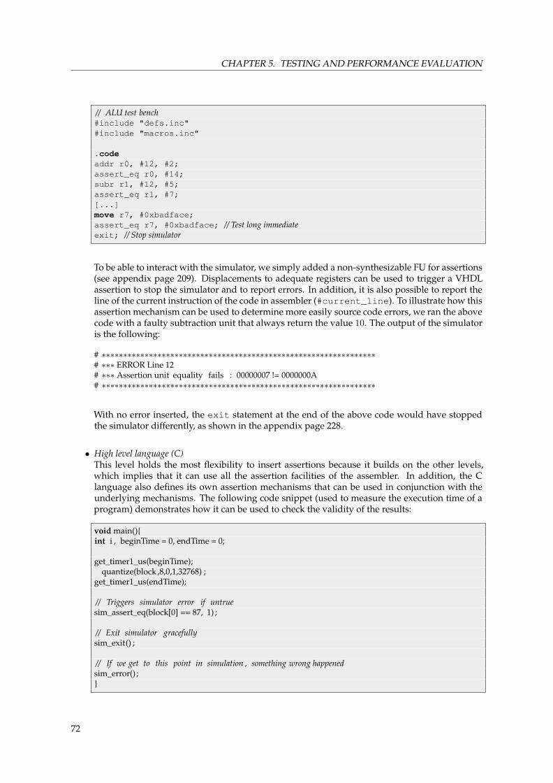
CHAPTER 5. TESTING AND PERFORMANCE EVALUATION

// ALU test bench#include "defs.inc"#include "macros.inc"

.codeaddr r0, #12, #2;assert_eq r0, #14;subr r1, #12, #5;assert_eq r1, #7;[...]move r7, #0xbadface;assert_eq r7, #0xbadface; // Test long immediateexit; // Stop simulator

To be able to interact with the simulator, we simply added a non-synthesizable FU for assertions(see appendix page 209). Displacements to adequate registers can be used to trigger a VHDLassertion to stop the simulator and to report errors. In addition, it is also possible to report theline of the current instruction of the code in assembler (#current_line). To illustrate how thisassertion mechanism can be used to determine more easily source code errors, we ran the abovecode with a faulty subtraction unit that always return the value 10. The output of the simulatoris the following:

# ∗∗∗∗∗∗∗∗∗∗∗∗∗∗∗∗∗∗∗∗∗∗∗∗∗∗∗∗∗∗∗∗∗∗∗∗∗∗∗∗∗∗∗∗∗∗∗∗∗∗∗∗∗∗∗∗∗∗∗∗∗∗∗∗# ∗∗∗ ERROR Line 12# ∗∗∗ Assertion unit equality fails : 00000007 != 0000000A# ∗∗∗∗∗∗∗∗∗∗∗∗∗∗∗∗∗∗∗∗∗∗∗∗∗∗∗∗∗∗∗∗∗∗∗∗∗∗∗∗∗∗∗∗∗∗∗∗∗∗∗∗∗∗∗∗∗∗∗∗∗∗∗∗

With no error inserted, the exit statement at the end of the above code would have stoppedthe simulator differently, as shown in the appendix page 228.

• High level language (C)This level holds the most flexibility to insert assertions because it builds on the other levels,which implies that it can use all the assertion facilities of the assembler. In addition, the Clanguage also defines its own assertion mechanisms that can be used in conjunction with theunderlying mechanisms. The following code snippet (used to measure the execution time of aprogram) demonstrates how it can be used to check the validity of the results:

void main(){int i , beginTime = 0, endTime = 0;

get_timer1_us(beginTime);quantize(block ,8,0,1,32768) ;

get_timer1_us(endTime);

// Triggers simulator error if untruesim_assert_eq(block[0] == 87, 1) ;

// Exit simulator gracefullysim_exit() ;

// If we get to this point in simulation , something wrong happenedsim_error() ;}

72

5.3. IN-CIRCUIT DEBUGGING

Fetchunit

Functionalunit

Functionalunit

Functionalunit

Functionalunit

DestinationSource

Data [31...0]

Memory

Debugunit

To the host system

Dest Src

Figure 5.1: Processor schematic with debug interface.

5.3 In-circuit debugging

The other testing technique we used in our design leverages the fact that every functional unit reactsto the destination and source buses on which the decoded instructions are placed. By temporarilyreplacing the fetch unit on these buses (Figure 5.1), it becomes possible to use all the FUs as indepen-dent modules. The debug unit represented in the same figure contains a few registers, that can beread or written from an external interface, offering a direct access to the FUs. This allows notably:

1. To read the content of every readable FU register (input and output). The whole internal state ofthe processor can thus be accessed and sent to the user to visualize the state of the system.

2. To modify the internal state of the processor by writing in the registers, for debugging purposes.It is thus possible to see the effects of the modification of a register on a program, which can beuseful during the development of programs.

3. To use the FUs without going through the fetch unit. This offers the possibility to realize compu-tations but also, in the situation where the processor contains an I/O interface, to interact withexternal hardware. This can be interesting for example in the case where the processor inter-faces a display, which can then be accessed from the CPU and from the debugging interface ina cooperative manner. Another possibility is to use the FUs only as hardware accelerators thatcan be easily accessed from a host computer.

The first point deserves a particular attention: whereas a standard processor requires to specificallyplan mechanisms (such as a JTAG interface3) to enable access to internal registers, in the case of a TTAprocessor the situation is much simpler. By taking into account this specificity, we have developed adebugger, similar to what many development environments offer.

This tool can be used during the development of programs by providing a faster and simple wayto examine execution, compared to simulation tools. However, it does not allow to examine more finedetails at the cycle level such as timings or fetch mechanisms.

The debugger itself can be called in-circuit, which signifies that it does not simulate but makes useof the finished processor inside a FPGA. It allows to check that the outcome of a program is what isexpected but also to verify that the FU in silico behave like in simulation.

At the hardware level, starting a debugging session corresponds to asserting the halt signal so thatthe processor goes to a state where the fetch unit releases control of the interconnection network andbehaves as a “slave” unit like the others. It is then possible to control the internal buses as would thefetch unit and thus read or write every register in the functional units by putting the correspondingaddresses on the buses. This mechanism can be used not only for debugging but also to modify thecontents of the memory.

3See http://www.jtag.com/.

73

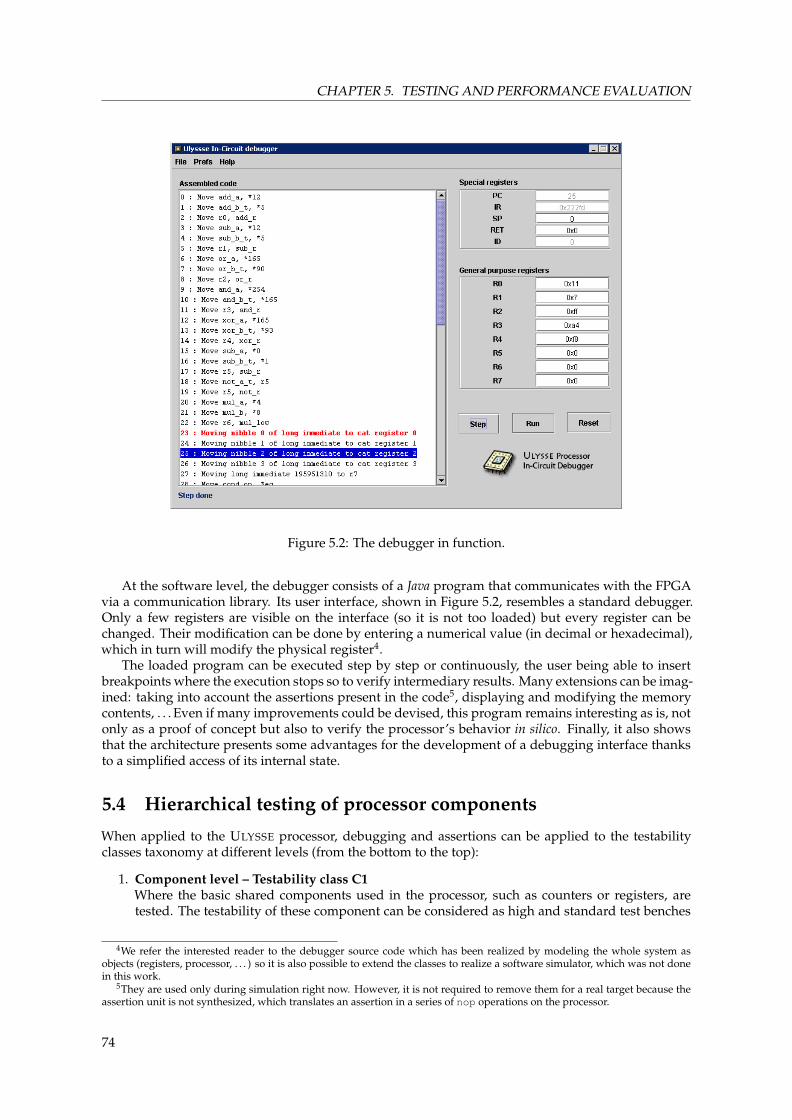
CHAPTER 5. TESTING AND PERFORMANCE EVALUATION

Figure 5.2: The debugger in function.

At the software level, the debugger consists of a Java program that communicates with the FPGAvia a communication library. Its user interface, shown in Figure 5.2, resembles a standard debugger.Only a few registers are visible on the interface (so it is not too loaded) but every register can bechanged. Their modification can be done by entering a numerical value (in decimal or hexadecimal),which in turn will modify the physical register4.

The loaded program can be executed step by step or continuously, the user being able to insertbreakpoints where the execution stops so to verify intermediary results. Many extensions can be imag-ined: taking into account the assertions present in the code5, displaying and modifying the memorycontents, . . . Even if many improvements could be devised, this program remains interesting as is, notonly as a proof of concept but also to verify the processor’s behavior in silico. Finally, it also showsthat the architecture presents some advantages for the development of a debugging interface thanksto a simplified access of its internal state.

5.4 Hierarchical testing of processor components

When applied to the ULYSSE processor, debugging and assertions can be applied to the testabilityclasses taxonomy at different levels (from the bottom to the top):

1. Component level – Testability class C1Where the basic shared components used in the processor, such as counters or registers, aretested. The testability of these component can be considered as high and standard test benches

4We refer the interested reader to the debugger source code which has been realized by modeling the whole system asobjects (registers, processor, . . . ) so it is also possible to extend the classes to realize a software simulator, which was not donein this work.

5They are used only during simulation right now. However, it is not required to remove them for a real target because theassertion unit is not synthesized, which translates an assertion in a series of nop operations on the processor.

74

5.4. HIERARCHICAL TESTING OF PROCESSOR COMPONENTS

that use equivalent test vectors and assertions can be easily used. In our implementation, thefollowing components have been tested using a dedicated test bench:

• generic width counter with settable count value;• generic width shift register with write enable signal;• generic width register with settable initial value;• the bus interface.

2. The functional unit level – Testability class C2Where the behavior of the different functional units is tested separately. Standard test benchescan be easily used, with the advantage that every functional unit can be plugged into similartest benches as they all have the same interface. If possible, for FUs that include other VHDLcomponents (such as IP modules), the external module was tested separately before being inte-grated. This was the case for example for the SRAM controller (section 3.7), which was testedwith asserted simulation and implemented independently to conduct functional testing. Theequivalence of test vectors can also be used to reduce the complexity of the test vectors.

3. The processor level – Testability class C3 / C4Where the global hardware behavior of the processor is tested. Testability at this level becomesmore complex because it requires code to execute, which also means external memory loading,bringing the code generated by the assembler into the simulator, simulation of the externalmemory with timings and CPU interactions . . . Equivalent test vectors are of little use to reducethe complexity of the tests but other debugging techniques can be used.Thus, debugging is done using the MODELSIMTM simulator where all the internal and exter-nal signals of the processor can be examined (see annex, page 229, Figure A.1). In addition tomanual examination of the results within the simulator, this level is also checked with assertedsimulation at all language levels along with debugging.This translates to a whole test suite written in assembler and C that contains test code for dif-ferent functionalities. This test suite is first checked in simulation, using a command-line en-vironment based on the MODELSIMTM interface. Because the GUI of MODELSIMTM is absent,simulations runs faster but at the expense of limited debugging possibilities, the only messagesprinted being those of the assertions in the code. A typical run of such a simulation is shown inannex page 228.The same testing suite can also be generated for an implemented version of the processor tocheck validity of the translation from the simulated model. With this suite, regressions are thussimplified and the correctness of new features can be asserted, following the idea proposedin [Meszaros 03] where systematic tests are used to validate code.As a side remark, we can also mention that test benches on the real platform were developed sothat physical interactions with the hardware are not required and code downloads fast. Thus,testing code only requires a key combination in our development environment, saving timeduring debugging.

4. The routing level – Testability class C4Networks On Chip will be introduced in a further chapter (section 8.3) and we only mention theproblematic here. Later in this work, tens of ULYSSE processors communicate together using aswitched network that dynamically creates communication paths. Testing such a setup requirescareful planning and is difficult, notably because of the highly irregular patterns that may ap-pear, which imply that very complex test vectors have to be generated. Moreover, because thenetwork spans different clock domains, clock relationships must also be considered. Achievinga good testability at this level is complex and requires considerable computational efforts (seefor example [Pande 05] or [Coppola 04] and section 8.3.2).

One advantage of using testability levels resides in the fact that it permits to handle the increasingcomplexity of each level because it builds atop a functionally working module. Of course, the imple-mentation of tests at each level requires a consequent time investment that, in our opinion, is largely

75

CHAPTER 5. TESTING AND PERFORMANCE EVALUATION

compensated by the fact that it becomes then possible to track problems very efficiently because thedifferent layers where the error can reside can be handled separately.

5.5 Processor validation, performance and results

Once a correct processor behavior was achieved, the next logical step was to evaluate and test theprocessor’s performance. To do so, several metrics that rely on different perspectives are possible:

Performance metrics To this category belong figures such as CPI, MIPS, Multiply-ACCumulate persecond. . . .

Single program tests This category contains figures that relate to standard program execution met-rics (such as number of standard blocks processed per second) that highlight different featuresof the processor to estimate its performance. Example of such programs are AES, RSA, imagekernel convolution, . . . .

Synthetic benchmarks This last category summarizes results from different programs (that mightbe contained in the second category above) to compute a benchmark score. The main advantageof this evaluation method is that it enables comparison between different platforms. However,because all the information is condensed into a single number, it might be hard to evaluate anarchitecture in detail. Examples of such benchmarks are the MEDIABENCH [Lee 97, Bishop 99]or EEMBC [Levy 05, Kanter 06], both targeted specifically to embedded processors. Often,other benchmarks (such as the SPEC6 suite) are used to estimate the general-purpose proces-sors present in desktop computers.

Testing and evaluating performance of a processor is a complex process because it involves manycomponents, not only hardware but also software, such as adequate compiler support for the archi-tecture. However, the purpose of this section is not to analyze the processor in depth so it can becompared with every other 32-bit processor available but to give an overview of the capabilities ofthe processor itself. Even when comparing ULYSSE with other similar processors, precautions haveto be taken when interpreting the differences. First, we have to consider that the GCC compiler forULYSSE does not yet support optimizations, which translates into big and inefficient code. Second,we also have to keep in mind that the main objective we pursued during the development of theprocessor was flexibility and not performance.

As a result, we propose in this section to evaluate the processor on several test programs thatcover different domains of computations spanned by embedded systems. Of course, using a com-plete benchmark such as DENBench that “[...] allows users to approximate the performance of processorsubsystems in multimedia tasks such as image, video, and audio file compression and decompression”7 wouldhave provided a better overview of the architecture, but this option was discarded because neither thesuite nor its source code are free and because the compiler is still under development. However, someprograms similar to test of the EEMBC suite could be written from scratch, the descriptions providedin documents such as [EEM 08] being clear enough to write a test program that captures the originalidea and were used for our test suite.

All the test programs were compiled using GCC in -O0 mode and, when possible, we also com-piled the programs for a NXP (founded by Philips) LPC2129 microcontroller8. This processor containsan ARM7TDMI-S core from ARM that can be clocked up to 60 MHz. Because the ARM GCC back-end allows optimizations, we compiled and measured size and execution of two versions of the ARMprogram, one with the same compilation options used with ULYSSE and one with optimization flagsset to -O3, which corresponds to maximum optimization.

The execution times on the ARM platform were measured using the internal high-precision timerthat provides a 0.1 µs resolution. A similar technique was used with the ULYSSE processor using the

6http://www.spec.org/7Taken from EEMBC website http://www.eembc.org/benchmark/digital_entertainment_sl.php8http://www.nxp.com/acrobat/datasheets/LPC2109_2119_2129_6.pdf

76

5.5. PROCESSOR VALIDATION, PERFORMANCE AND RESULTS

timer FU, however with a resolution limited to 1 µs. The code template that was used in both casescan be found in the appendix of this document (see section A.7, page 230).

5.5.1 Description of the benchmark suite

We describe in this section the programs that were used to estimate ULYSSE’s performance in domainssuch as multimedia, with video compression or image filtering, or more general purpose, such assorting. Before that, we need to introduce the notion of acceleration factor, which will be used tocompare the performance of programs when executed on different platforms.

Definition If we consider a program p, ta(p) its execution time within CPUa and tb(p) its executiontime within CPUb, the acceleration factor γ can be considered as:

γba(p) =ta(p)tb(p)

(5.1)

The benchmark suite contains the following programs:

FDCT The forward discrete cosine transform (FDCT) program works on 8x8 image (8 bits deep)blocks. FDCT is a common operation in image compression where it is used to extract themost significant frequency components of an image block.

IDCT The inverse operation of the FDCT that allows the transformation from the frequency domainto the spatial domain.

VLC Variable-length coding (VLC) is a compression scheme used to encode blocks of data, for ex-ample coefficients blocks in the JPEG algorithm or inter-block motion vectors in MJPEG. Thesample application compresses an array of 128x32 bits of data.

IVLC Inverse variable-length coding (IVLC). This is the inverse function of VLC that transformscompressed data to uncompressed ones. Produces an array of 128x32 bits of data.

High pass greyscale filtering This is a sharpening filter (convolution kernel) that exploits CPU mem-ory accesses and MACC operations. In this sample application, it processes 3x3 gray-scale imageblocks.

Quantization Digital signal processing technique that reduces the information to be encoded usingsymbols. Used to perform VLC in image compression for example. The sample applicationworks on a 8x8 data matrix.

RGB to CMYK Color space conversion that consists in transforming Red–Green–Blue (RGB) colorcoded samples into the Cyan-Magenta-Yellow-blacK (CMYK) colors used in the printing indus-try or in printers. The arithmetic operations used for this transformation are basic ones suchas subtraction along with minima extraction. The image sample is an RGB 100x10 image. Thetransformation algorithm is based on the EEMBC databook [EEM 08].

RGB to YUV Color space conversion used in the video reproduction of colors in which RGB samplesare transformed in a color space with one luma (Y) and two chrominance components (UV),used for example in the NTSC or PAL video standards. The algorithm’s input is an 8x8 RGBsample.

Bubble sort Standard sorting algorithm with complexity O(n2), n being the number of elements tosort. In this application sample, an inversely-sorted list of n elements has to be sorted, whichconstitutes the worst execution time for the algorithm.

FIR Finite Impulse Response filter (FIR) is a type of digital filter that is commonly used in digitalsignal processing. Its general form is y[n] =

∑Ni=0 bix[n−i] and theN+1 elements that compose

the right-hand side of the equation are referred as taps.

77

CHAPTER 5. TESTING AND PERFORMANCE EVALUATION

1

10

100

1000

10000

100000

1000000

Exec

uti

on

tim

e [µ

s]

Ulysse

ARM7 ( -O0)

ARM7 ( -O3)

FDCT

High p

assID

CTIV

LC

Quantizatio

n

RGB2YUV

RGB2CMYK

VLC

Bubble(mean)

FIR(m

ean)

(a) Program performance for each considered architecture

500 1000 1500 2000 2500 3000 3500 4000

0

2000

4000

6000

8000

10000

12000

14000

16000

18000

Execution time [µs]

Exec

uti

on

tim

e [µ

s]

Ulysse vs. ARMLinear regression

Linear model f(x) = p1 x + p2

Coefficients p1 = 4.025 p2 = −366.9

(b) Linear regression of ULYSSE versus ARM7 performance

Figure 5.3: Performance measures on various programs.

78

5.5. PROCESSOR VALIDATION, PERFORMANCE AND RESULTS

Sample program pExecution time [µs] Acceleration factor

ULYSSEa ARM7b (-O0) ARM7c (-O3) γba(p) γc

b (p)

FDCT 910 260.31 67.33 3.50 3.86High pass 4607 1412.91 23.54 3.26 60.02IDCT 1026 275.15 96.15 3.73 2.85IVLC 12359 3579.03 818.82 3.45 4.37Quantization 1045 283.23 65.36 3.69 4.33RGB to YUV 1561 413.26 5.5 3.77 75.14RGB to CMYK 17994 4002.77 83.52 4.49 47.93VLC 5847 1855.25 638.46 3.15 2.9

Bubble sort [50]a 10168 2309.5 443.0Bubble sort [100] 40836 9243.3 1760.9Bubble sort [200] 153445 36985.8 7021.7Bubble sort [400] 655338 147964.1 28010.2Bubble average 214947 49125.67 9308.95 4.37 5.27

FIR[1]FIR[2] 124 33.68 2.33FIR[4] 211 56.76 4.00FIR[6] 284 76.98 5.66FIR[8] 346 94.33 7.33FIR average 208 56.56 3.96 3.66 14.26

aThe parameter corresponds to the size of the list to be sorted.

Table 5.1: Performance measures on various programs.

The results of the performance evaluation are summarized in Table 5.1 with more details for theFIR and bubble sort programs because their performance depend on the number of elements of theworking set presented.

In Figure 5.3a, it clearly appears that the performance of the ARM7 platform is better but also thatcompiler optimizations can be really effective sometimes. Concerning the comparison of the ARM7and ULYSSE, as can be seen in Table 5.1, for each program p, the γba(p) value remains relatively stable.On average, ULYSSE is 3.7 times slower (with standard deviation σ = 0.43) than the ARM7TDMI pro-cessor. A further analysis of the performance, done with a linear regression9, depicted in Figure 5.3b,yields a similar estimated ratio (4.025) between the two processors. Even if ULYSSE is outperformedby another CPU, we still consider that this constitutes a reasonable result considering the following:

• The focus was put during the development of the processor on flexibility and correct behaviorrather than raw performance.

• The dual-chip, interleaved memory PCB design requires twice the number of cycles anotherwiring would allow. In other words, using a 32-bit bus instead of 2x16 bits for memory dataaccess would greatly improve the processor performance (at least by 33%).

• The architecture, in and for itself, does not necessarily imply performance as its major advantage.This is especially true when no VLIW instructions are used because a simple operation takesmultiple instructions in TTA, hence the slower execution time. Moreover, GCC generated codefor ULYSSE does not make use of any architectural optimizations.

• ULYSSE is clocked 20% slower than the particular ARM7 CPU used, notably because it does notbenefit from a VLSI implementation as it is the case for the ARM710.

9Bubble sort and FIR programs were not taken into account for this regression.10A more complete comparison would need to take into account power consumption, silicium size, etc. However, an estima-

tion of ULYSSE’s parameters for VLSI was not possible because we did not possess adequate synthesis tools.

79

CHAPTER 5. TESTING AND PERFORMANCE EVALUATION

5.6 Code size comparisons

Sample program pCode size [bytes]

ULYSSE ARM7 (-O0)

FDCT 6524 3984High pass 3580 3060IDCT 16724 7668IVLC 17524 5928Quantization 3848 3240RGB to YUV 2132 1696RGB to CMYK 1900 1552VLC 13816 5752Bubble sort 5524 4328FIR 1524 2388

Table 5.2: Code size measurements.

Besides execution time, code size also plays an important role in embedded systems. For this rea-son, we will now compare the code sizes of the same programs on the ULYSSE and ARM7 platforms11.

6524 3580 16724 17524 3848 2132 1900 13816 5524 1524

3894

3060

7668

5928

3240 1696 1552

5752

4328

2388

0%

10%

20%

30%

40%

50%

60%

70%

80%

90%

100%

FDCT High pass IDCT IVLC Quantization RGB2YUV RGB2CMYK VLC Bubble sort FIR

Ulysse ARM

Figure 5.4: Comparison of different program sizes.

Table 5.2 shows the respective code sizes whereas Figure 5.4 depicts a side-by-side comparisonof the two compiled codes for each program. On average, ULYSSE code size in our experiments islarger (on average 1.59 times, standard deviation σ = 0.70) than the ARM version when using thesame compiler in the same conditions. Unfortunately, even if it would be interesting to compare thesize-optimized versions for both architectures, it is impossible because ULYSSE GCC version does notallow this optimization yet.

It would also be interesting to be able to compare with another processor architecture that tends toovergrow code, such as VLIW, to see how the code increase compares as was done in [Heikkinen 02].

11Because the execution times of the ARM7 were collected via a terminal using printf() statements, we had to removethem in the size measurements to achieve a fair comparison.

80

5.7. COMPARING SIMULATION AND EXECUTION TIMES

5.7 Comparing simulation and execution times

We have at our disposal two different methods to determine the execution time of a program on theULYSSE processor, namely simulation and measure. The advantage of the first method resides in the factthat a real execution platform is not needed to perform measures but also in the fact that the internalsignals of the processor can be examined at each execution step thanks to the simulator’s display. Onthe other hand, the second approach overcomes the limitation of the long evaluation times exhibitedby the simulator by providing a real-time measure of the execution time.

Sample program Simulated exec. time [µs] Execution time [µs] Simulation time [s]

Quantization 1047.580 1045 95IDCT 1026.82 1026 92

Bubble[5]a 97.36 96 5Bubble[10] 396.56 395 21Bubble[15] 900.76 899 43Bubble[20] 1610 1609 83

FIR[1]b 76.8 75 5FIR[2] 124.8 124 6FIR[8] 346.72 346 17

aThe parameter corresponds to the size of the list to be sorted.bThe parameter corresponds to the number of taps to realize.

Table 5.3: Simulation and execution times.

To demonstrate the validity of the simulation environment measurements, Table 5.3 shows the ex-ecution times estimated with the simulator and the measured execution times of some programs. Inthe same table, an approximate12 simulation time is shown for each test program, clearly demonstrat-ing that, even if complete simulation remains an interesting solution notably to discover errors in thecode, it is a relatively slow process.

5.8 Conclusion

The goal of designing a functional, compiler-supported processor was met. A respectable perfor-mance was obtained, as evidenced by the benchmark suite, even if further work on the compiler portto enable the complete spectrum of GCC optimizations would drastically increase the global perfor-mance. Another possibility to improve performance would be to use a different memory PCB layout,a change that would directly translate in doubling the performance.

More importantly, the ULYSSE processor provides a stable and well-tested platform that remainswidely open to further enhancements. With the robust software support, validated with complexapplications, our processor will be used in this thesis for two main purposes:

1. We will show in the next chapter that the flexibility of processor can be further harvested byautomatically developing ad-hoc functional units to adapt the processor to different programs.Thanks to a genetic algorithm, we will evolve the processor in order to accelerate computation inhardware.

2. The ULYSSE processor will be used in the second half of this work as a building block for amassively parallel hardware platform, which will be described starting in chapter 8.

12Exact measures are almost impossible, since the simulator does not always return the same measure for the two identicalexperiments. We estimate the precision to be in the order of ±5 seconds.

81

Bibliography

[Bishop 99] Benjamin Bishop, Thomas P. Kelliher & Mary Jane Irwin. A detailed analysis of Media-Bench. In Proceedings of the IEEE Workshop on Signal Processing Systems (SiPS’99),pages 448–455, 1999.

[Boule 05] Marc Boule & Zeljko Zilic. Incorporating Efficient Assertion Checkers into Hardware Em-ulation. In Proceedings of the 2005 International Conference on ComputerDesign(ICCD’05), pages 221–228, Washington, USA, 2005. IEEE Computer Society.

[Coppola 04] Marcello Coppola, Stephane Curaba, Miltos D. Grammatikakis, Riccardo Locatelli,Giuseppe Maruccia & Francesco Papariello. OCCN: a NoC modeling framework for de-sign exploration. Journal of Systems Architecture, vol. 50, no. 2-3, pages 129–163, 2004.

[EEM 08] EEMBC. DENBench 1.0 – Software benchmark databook, 2008. http://www.eembc.org/techlit/datasheets/denbench_db.pdf.

[Eisner 06] Cindy Eisner & Dana Fisman. A Practical Introduction to PSL. Series on IntegratedCircuits and Systems. Springer-Verlag New York, Inc., Secaucus, NJ, USA, 2006.

[Foster 03] Harry Foster, David Lacey & Adam Krolnik. Assertion-Based Design. Kluwer Aca-demic Publishers, Norwell, MA, USA, 2003.

[Foster 05] Harry Foster, E. Marschner & D. Shoham. Introduction to PSL. Springer-Verlag NewYork, Inc., Secaucus, NJ, USA, 2005.

[Heikkinen 02] J. Heikkinen, J. Takala, A. G. M. Cilio & H. Corporaal. On efficiency of transport triggeredarchitectures in DSP applications, pages 25–29. N. Mastorakis, January 2002.

[Kanter 06] David Kanter. EEMBC Energizes Benchmarking. Microprocessor Report, vol. 1, pages1–7, July 2006.

[Lee 97] Chunho Lee, Miodrag Potkonjak & William H. Mangione-Smith. MediaBench: a toolfor evaluating and synthesizing multimedia and communicatons systems. In MICRO 30:Proceedings of the 30th annual ACM/IEEE international symposium on Microarchi-tecture, pages 330–335, Washington, USA, 1997. IEEE Computer Society.

[Levy 05] Markus Levy. Evaluating Digital Entertainment System Performance. Computer, vol. 38,no. 7, pages 68–72, 2005.

[Meszaros 03] G. Meszaros, S. M. Smith & J. Andrea. The Test Automation Manifesto, vol. 2753 of Lec-ture Notes in Computer Science, pages 73–81. Springer Berlin / Heidelberg, September2003.

[Pande 05] Partha Pratim Pande, Cristian Grecu, André Ivanov, Resve Saleh & Giovannide Micheli. Design, Synthesis, and Test of Network on Chips. IEEE Design & Test ofComputers, vol. 22, no. 5, pages 404–413, 2005.

83

Chapter 6

Processor evolution

“Le seul mauvais choix est l’absence de choix.”

AMÉLIE NOTHOMB, La métaphysique des tubes

ULYSSE’s main strength resides in its capability to easily accommodate changes in its operationset. As such, it can easily adapt to different kind of computations through its FU-based modular

approach. However, in the system described in the previous chapters, the work of determining whichFUs are pertinent to realize a given computation is left to the user. In this chapter, we will see thatthis process of adapting the processor to a particular application can be automated by using a geneticalgorithm (GA), a process that not only determines which FUs to include, but also proposes new FUsif necessary.

6.1 Introduction and motivations

As very efficient heuristics, genetic algorithms have been widely used to solve complex optimizationproblems. However, when the search space to be explored becomes very large, this technique becomesinapplicable or, at least, inefficient. This is the case when GAs are applied to the partitioning problem,which is one of the tasks required for the hardware-software codesign of embedded systems.

Consisting in the concurrent realization of the hardware and the software layers of an embeddedsystem, codesign has been used since the early nineties and is now a technique widely spread inthe industry. This design methodology permits to exploit the different synergies of hardware andsoftware that can be obtained for a particular embedded system. Such systems are usually builtaround a core processor that can be connected to hardware modules tailored for a specific application.This “tailoring” corresponds to the codesign of the system and consist in different tasks, as definedin [Harkin 01]: partitioning, co-synthesis, co-verification and co-simulation.

In this chapter, we will focus on the complex, NP-complete [Oudghiri 92], partitioning problemthat can be defined as follows: starting from a program to be implemented on a digital system andgiven a certain execution time and/or size constraints, the partitioning task consists in the determina-tion of which parts of the algorithm have to be implemented in hardware in order to satisfy the givenconstraints.

As this problem is not new, several methods have been proposed in the past to solve it: Gupta andde Micheli start with a full hardware implementation [Gupta 92], whilst Ernst et al. [Ernst 93,Ernst 02]use profiling results in their COSYMA environment to determine with a simulated annealing algorithmwhich blocks to move to hardware. Vahid et al. [Vahid 94] use clustering together with a binary-constrained search to minimize hardware size while meeting constraints. Others have proposed ap-proaches such as fuzzy logic [Catania 97], genetic algorithms [Dick 98, Srinivasan 98], hierarchicalclustering [Hou 96] or tabu search [Eles 97, Ahmed 04] to solve this task.

We chose to work with a genetic algorithm because of the complex nature of the partitioning taskbut also because partitioning enables the usage of program trees as data structures, a very convenient

85

CHAPTER 6. PROCESSOR EVOLUTION

data type to apply genetic programming (see [Koza 92]). Although some attempts to use genetic al-gorithms have been shown to be less efficient than other techniques such as simulated annealing tosolve the partitioning task [Wiangtong 04, Wiangtong 02], they can be hybridized to take into accountthe particularities of the problem and solve it efficiently.

The improved genetic algorithm we propose starts from a software tree representation and pro-gressively builds a partition of the problem by looking for the best compromise between raw perfor-mance and hardware area increase. In other words, it tries to find the most interesting parts of theinput program to be implemented in hardware, given a limited amount of resources.

The novelty of our approach lies in the several optimizations passes applied to the intermediaryresults of a standard GA, which allows to avoid the most common pitfalls associated with GAs, suchas being trapped in local minima, thanks to a dynamically-weighted fitness function. Thus, we obtainan hybridized algorithm that explores only the most interesting parts of the solution space and, whengood candidates are found, refines them as much as possible to extract their potential. Finally, wewill show that our algorithm is robust and performs well on relatively large programs by quicklyconverging to good solutions.

This chapter is organized as follows: in the next section we formulate the problem in the contextof a genetic algorithm and section 6.4 describes the specific enhancements that are applied to thestandard GA approach. Afterwards, we present some experimental results which show the efficiencyof our approach. Finally, section 6.8 concludes this chapter and introduces future work.

6.2 Partitioning with TTA

We have developed our new partitioning method in the context of the Move processor paradigmbut our approach remains general and could be used for different processor architectures and variousreconfigurable systems with only minor changes. However, the fact that TTAs handle functional unitsas “black boxes”, i.e. without any inherent knowledge of their functionality, implies that the internalarchitecture of the processor can be described as a memory map which associates the different possibleoperations with the addresses of the corresponding functional units. As a result, implementing newFUs is simpler than in other architectures.

Because of the versatility of such processors, automatic partitioning becomes indeed very interest-ing for the synthesis of ontogenetic, application-specific processors: the partitioning can automaticallydetermine which parts of the code of a given program are the best candidates to be implemented asFUs. The algorithm described in this chapter introduces in our global framework a way to automat-ically specializing the instruction set (i.e., defining ad-hoc functional units) to the application whilekeeping the overall structure of the processor unchanged.

6.3 A basic genetic algorithm for partitioning

We describe in this section the basic GA that serves as a basis for our partitioning method and thatwill be enhanced in section 6.4 with TTA-specific improvements. The basic algorithm, whose flowdiagram is depicted in Figure 6.1, works as follows: starting from a program written in a specificlanguage resembling C, a syntactic tree is built and then analyzed by the GA, which then produces avalid, optimized partition. The various parameters of the GA can be specified on the graphical userinterface that has been designed, like all other software described in this section, in Java.

6.3.1 Programming language and profiling

Assembly could have been used as an input for our algorithm but the general structure of a Moveassembly program is difficult to capture because every instruction is considered only as a data dis-placement, introducing a great deal of complexity in the representation of the program’s functionality.Thus, the programs to be evolved by the GA are written in a simplified programming language thatsupports all the classical declarative language constructs in a syntax resembling C. Several limitationshave however been imposed to this programming language:

86

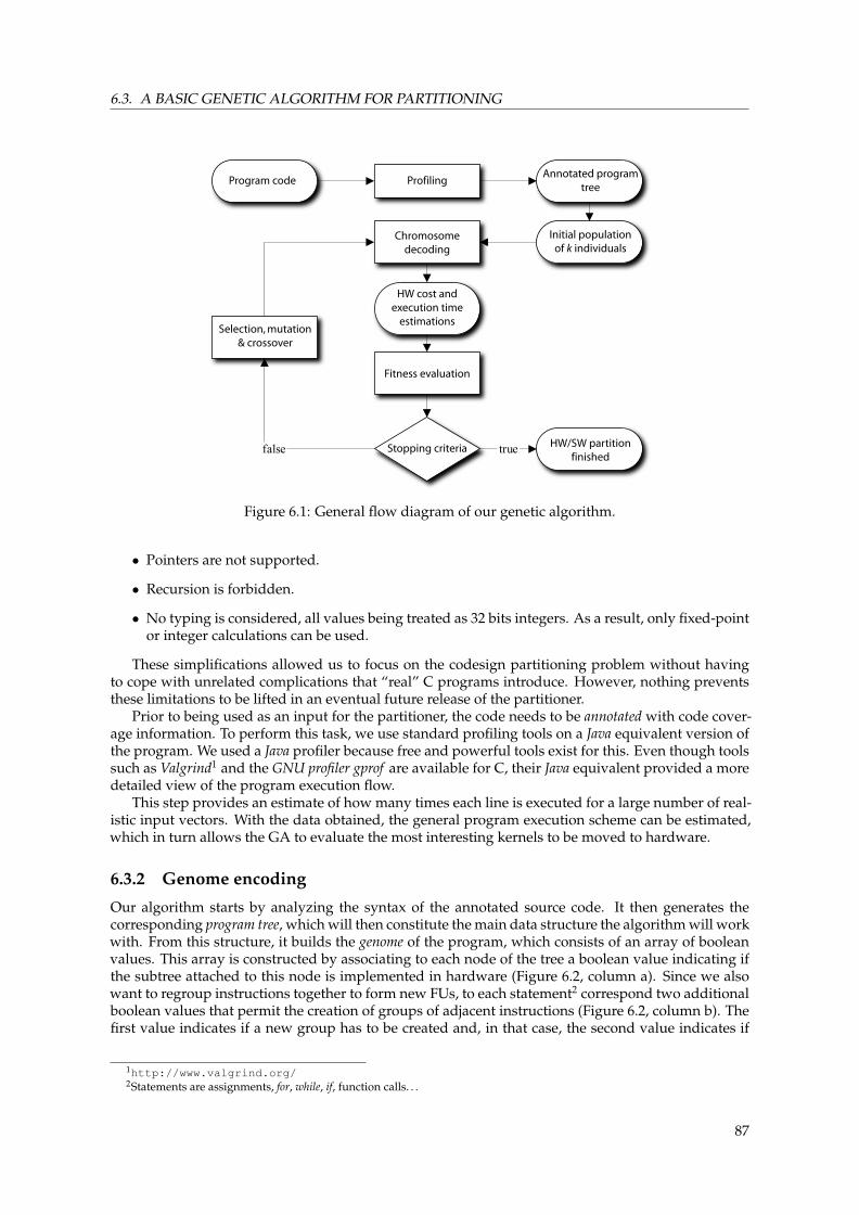
6.3. A BASIC GENETIC ALGORITHM FOR PARTITIONING

false true

Program codeAnnotated program

treeProfiling

Initial populationof k individuals

Chromosomedecoding

HW cost andexecution time

estimations

Fitness evaluation

Stopping criteria HW/SW partitionfinished

Selection, mutation& crossover

Figure 6.1: General flow diagram of our genetic algorithm.

• Pointers are not supported.

• Recursion is forbidden.

• No typing is considered, all values being treated as 32 bits integers. As a result, only fixed-pointor integer calculations can be used.

These simplifications allowed us to focus on the codesign partitioning problem without havingto cope with unrelated complications that “real” C programs introduce. However, nothing preventsthese limitations to be lifted in an eventual future release of the partitioner.

Prior to being used as an input for the partitioner, the code needs to be annotated with code cover-age information. To perform this task, we use standard profiling tools on a Java equivalent version ofthe program. We used a Java profiler because free and powerful tools exist for this. Even though toolssuch as Valgrind1 and the GNU profiler gprof are available for C, their Java equivalent provided a moredetailed view of the program execution flow.

This step provides an estimate of how many times each line is executed for a large number of real-istic input vectors. With the data obtained, the general program execution scheme can be estimated,which in turn allows the GA to evaluate the most interesting kernels to be moved to hardware.

6.3.2 Genome encoding

Our algorithm starts by analyzing the syntax of the annotated source code. It then generates thecorresponding program tree, which will then constitute the main data structure the algorithm will workwith. From this structure, it builds the genome of the program, which consists of an array of booleanvalues. This array is constructed by associating to each node of the tree a boolean value indicating ifthe subtree attached to this node is implemented in hardware (Figure 6.2, column a). Since we alsowant to regroup instructions together to form new FUs, to each statement2 correspond two additionalboolean values that permit the creation of groups of adjacent instructions (Figure 6.2, column b). Thefirst value indicates if a new group has to be created and, in that case, the second value indicates if

1http://www.valgrind.org/2Statements are assignments, for, while, if, function calls. . .

87

CHAPTER 6. PROCESSOR EVOLUTION

{while(a < 10){…}b = c << 1;foo(d);d = d % 3;if(b < 3){…};}

1100100011

(a) (b)

while(a < 10){…}b = c << 1;

HW Group 1

foo(d);d = d % 3; HW

SW Group 1

if(b < 3){…};

11010

Instruction is HW/SWCreate group

Group is HW/SW

Code Genome

HW Group 2

Figure 6.2: Genome encoding.

the whole group has to be implemented in hardware (i.e. to create a new FU). The complete genomeof the program is then formed by the concatenation of the genomes of the single nodes.

Soft group

Hard group

Hardware group

root

=

0 00

if

0 10

while

1 11

*

0a

==

0...

!=

1...

c 24+

1b

d 1

e 30

if(c == 24) {...};a = b * (d+1);while(e != 30) {...};

Figure 6.3: Creation of groups according to the genome.

An example of a program tree with its associated genome is represented in Figure 6.3, whichdepicts the different possible groupings and the representation of the data the algorithm works with.

6.3.3 Genetic operators

When GA are used, several genetic operators are applied (see Figure 6.4). In our approach, we useoperators inspired from [Koza 92], i.e. selection, mutation and crossover.

88

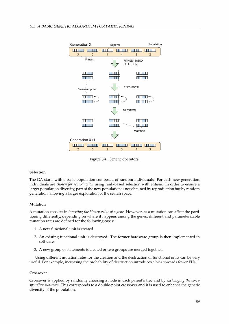
6.3. A BASIC GENETIC ALGORITHM FOR PARTITIONING

3 5 1 4 3 2

2 6 2 5 4 3

Generation X

Generation X+1

Mutation

MUTATION

CROSSOVER

FITNESS-BASEDSELECTION

Fitness

Crossover point

PopulationGenome

Figure 6.4: Genetic operators.

Selection

The GA starts with a basic population composed of random individuals. For each new generation,individuals are chosen for reproduction using rank-based selection with elitism. In order to ensure alarger population diversity, part of the new population is not obtained by reproduction but by randomgeneration, allowing a larger exploration of the search space.

Mutation

A mutation consists in inverting the binary value of a gene. However, as a mutation can affect the parti-tioning differently, depending on where it happens among the genes, different and parameterizablemutation rates are defined for the following cases:

1. A new functional unit is created.

2. An existing functional unit is destroyed. The former hardware group is then implemented insoftware.

3. A new group of statements is created or two groups are merged together.

Using different mutation rates for the creation and the destruction of functional units can be veryuseful. For example, increasing the probability of destruction introduces a bias towards fewer FUs.

Crossover

Crossover is applied by randomly choosing a node in each parent’s tree and by exchanging the corre-sponding sub-trees. This corresponds to a double-point crossover and it is used to enhance the geneticdiversity of the population.

89

CHAPTER 6. PROCESSOR EVOLUTION

6.3.4 Fitness evaluation

Determining hardware size and execution time

Computing hardware size and execution time is one of the key aspects of the algorithm, as it definesthe fitness of an individual which then influences the choice of whether an evolved solution will bekept or not. Different techniques exist to determine these values, for example [Henkel 98] or [Vahid 95]and, more recently, [Pitkänen 05]. The method we chose to use is based on a very fine characteriza-tion of each hardware elementary building block of the targeted hardware platform which, in theimplementation discussed here, is a Xilinxr VIRTEXTM II-3000 field-programmable gate array.

The characterization of each of these building blocks, which carry out very simple logical andarithmetic operations (AND, OR, +, . . . ), allows then to arrange them together to elaborate more com-plex operations that form new FUs in the Move processor. For example, it is possible to reduce theexecution of several software instructions to only one clock cycle by chaining them in hardware, asdepicted in Figure 6.5 (note that the shift operation used in the example is “free” in hardware, i.e. noslices3 are used, because only wires are required to achieve the same result). This simple exampleshows the principles of how the basic blocks are chained and how hardware size and execution timeare predicted.

And32 slices

<20 slices Free slot

Clock period @ 100 MHz

Instruction: ((a << 2) and 4) < 0xFFExecution time : 2.98 nsHardware area needed: 52 slices

0.38 ns 2.60 ns0 ns

Figure 6.5: Hardware time and size estimation principle of a 32-bit software instruction.

The basic blocks’ size and timing metrics have been determined using the SYNPLIFY PROTM syn-thesis solution coupled, in some cases, with the Xilinxr place-and-route tools. Thus, we have ob-tained the number of slices of the FPGA required to implement each block and the length of thecritical path of each basic block. Because this characterization mostly depends on the architecturetargeted and on the software used, it has to be redone for each different hardware platform targeted.This very detailed characterization permitted us to take into account a wide range of timings, fromsub-cycle estimates for combinational operators to multi-cycle estimates for high latency operatorssuch as pipelined dividers. Area estimators were built using the same principles. Using these param-eters, determining size and time for each sub-tree is then relatively straightforward because only twodifferent cases have to be considered:

1. For software sub-trees, the estimation is done recursively over the nodes of the program tree,adding at each step the appropriate execution time and potential hardware unit: e.g. the firsttime an add instruction is encountered, an add FU must be added to compose the minimalprocessor necessary to execute this program.

2. For hardware sub-trees, the computation is a bit more complex because it depends on the po-sition of the considered sub-tree: if it is located at the root of a group, it constitutes a new FUand some computation is needed. In fact, the time to move the data to the new FU and thesize of the registers required for the storage of the local variables have to be taken into account.

3Slices are the fundamental elements of the FPGA. They roughly characterize how much space for logic is available on agiven circuit. The name and implementation of these elements differ from one hardware vendor to one another.

90

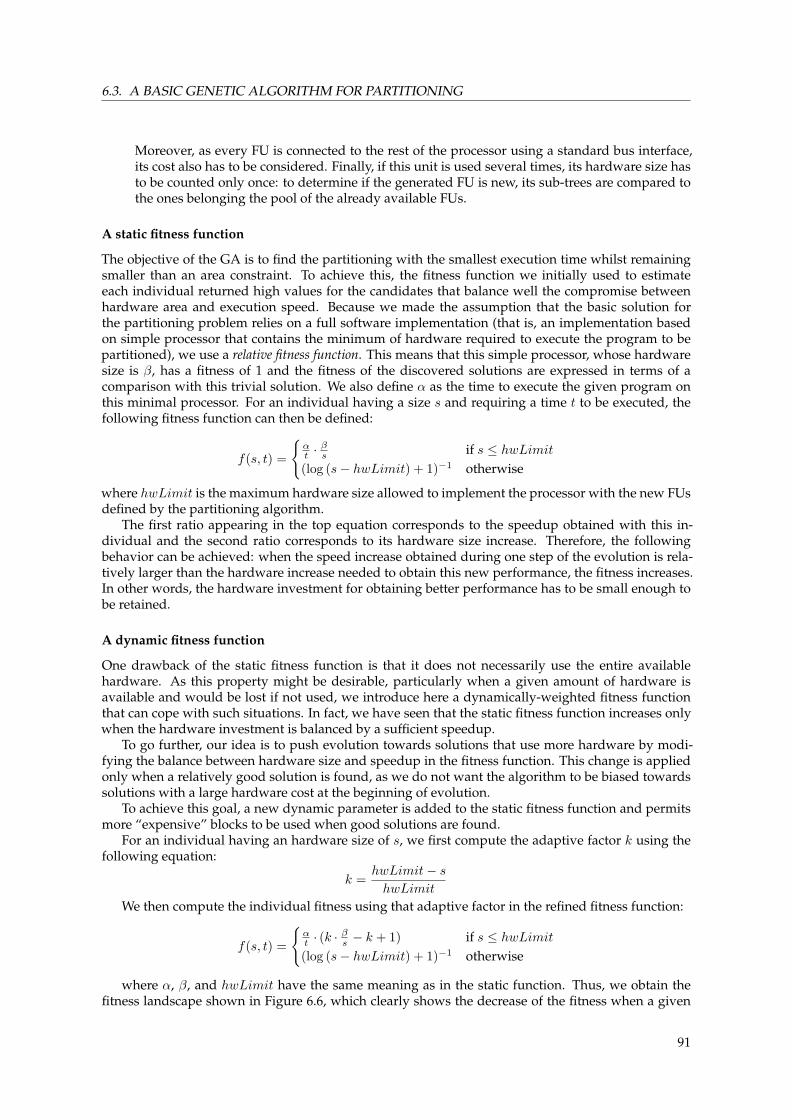
6.3. A BASIC GENETIC ALGORITHM FOR PARTITIONING

Moreover, as every FU is connected to the rest of the processor using a standard bus interface,its cost also has to be considered. Finally, if this unit is used several times, its hardware size hasto be counted only once: to determine if the generated FU is new, its sub-trees are compared tothe ones belonging the pool of the already available FUs.

A static fitness function

The objective of the GA is to find the partitioning with the smallest execution time whilst remainingsmaller than an area constraint. To achieve this, the fitness function we initially used to estimateeach individual returned high values for the candidates that balance well the compromise betweenhardware area and execution speed. Because we made the assumption that the basic solution forthe partitioning problem relies on a full software implementation (that is, an implementation basedon simple processor that contains the minimum of hardware required to execute the program to bepartitioned), we use a relative fitness function. This means that this simple processor, whose hardwaresize is β, has a fitness of 1 and the fitness of the discovered solutions are expressed in terms of acomparison with this trivial solution. We also define α as the time to execute the given program onthis minimal processor. For an individual having a size s and requiring a time t to be executed, thefollowing fitness function can then be defined:

f(s, t) =

{αt ·

βs if s ≤ hwLimit

(log (s− hwLimit) + 1)−1 otherwise

where hwLimit is the maximum hardware size allowed to implement the processor with the new FUsdefined by the partitioning algorithm.

The first ratio appearing in the top equation corresponds to the speedup obtained with this in-dividual and the second ratio corresponds to its hardware size increase. Therefore, the followingbehavior can be achieved: when the speed increase obtained during one step of the evolution is rela-tively larger than the hardware increase needed to obtain this new performance, the fitness increases.In other words, the hardware investment for obtaining better performance has to be small enough tobe retained.

A dynamic fitness function

One drawback of the static fitness function is that it does not necessarily use the entire availablehardware. As this property might be desirable, particularly when a given amount of hardware isavailable and would be lost if not used, we introduce here a dynamically-weighted fitness functionthat can cope with such situations. In fact, we have seen that the static fitness function increases onlywhen the hardware investment is balanced by a sufficient speedup.

To go further, our idea is to push evolution towards solutions that use more hardware by modi-fying the balance between hardware size and speedup in the fitness function. This change is appliedonly when a relatively good solution is found, as we do not want the algorithm to be biased towardssolutions with a large hardware cost at the beginning of evolution.

To achieve this goal, a new dynamic parameter is added to the static fitness function and permitsmore “expensive” blocks to be used when good solutions are found.

For an individual having an hardware size of s, we first compute the adaptive factor k using thefollowing equation:

k =hwLimit− shwLimit

We then compute the individual fitness using that adaptive factor in the refined fitness function:

f(s, t) =

{αt · (k ·

βs − k + 1) if s ≤ hwLimit

(log (s− hwLimit) + 1)−1 otherwise

where α, β, and hwLimit have the same meaning as in the static function. Thus, we obtain thefitness landscape shown in Figure 6.6, which clearly shows the decrease of the fitness when a given

91

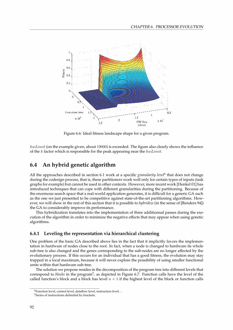
CHAPTER 6. PROCESSOR EVOLUTION

[slices]

Figure 6.6: Ideal fitness landscape shape for a given program.

hwLimit (on the example given, about 19000) is exceeded. The figure also clearly shows the influenceof the k factor which is responsible for the peak appearing near the hwLimit.

6.4 An hybrid genetic algorithm

All the approaches described in section 6.1 work at a specific granularity level4 that does not changeduring the codesign process, that is, these partitioners work well only for certain types of inputs (taskgraphs for example) but cannot be used in other contexts. However, more recent work [Henkel 01] hasintroduced techniques that can cope with different granularities during the partitioning. Because ofthe enormous search space that a real-world application generates, it is difficult for a generic GA suchas the one we just presented to be competitive against state-of-the-art partitioning algorithms. How-ever, we will show in the rest of this section that it is possible to hybridize (in the sense of [Renders 94])the GA to considerably improve its performance.

This hybridization translates into the implementation of three additionnal passes during the exe-cution of the algorithm in order to minimize the negative effects that may appear when using geneticalgorithms.

6.4.1 Leveling the representation via hierarchical clustering

One problem of the basic GA described above lies in the fact that it implicitly favors the implemen-tation in hardware of nodes close to the root. In fact, when a node is changed to hardware its wholesub-tree is also changed and the genes corresponding to the sub-nodes are no longer affected by theevolutionary process. If this occurs for an individual that has a good fitness, the evolution may staytrapped in a local maximum, because it will never explore the possibility of using smaller functionalunits within that hardware sub-tree.

The solution we propose resides in the decomposition of the program tree into different levels thatcorrespond to blocks in the program5, as depicted in Figure 6.7. Function calls have the level of thecalled function’s block and a block has level n + 1 if the highest level of the block or function calls

4Function level, control level, dataflow level, instruction level. . .5Series of instructions delimited by brackets.

92

6.4. AN HYBRID GENETIC ALGORITHM

foo ( val ) { return val + 1 ; }

main () { if ( c == 24 ) { …

}; a = b *( d + 1 ) ; while ( e < 30 ) { foo ( d ) ;

… }; }

level 0

level 1

level 2

level 0

Figure 6.7: Levels definition.

it contains is n, the deepest blocks being at level 0 by definition. These levels represent interestingpoints of separation because they often correspond to the most computationally intensive parts of theprograms (e.g. loops) that are good candidates for being implemented in new FUs.

To circumvent the creation of ill-sized blocks, the GA is recursively applied to each level, startingwith the deepest ones (n = 0). To pass information between each level, the genome of the bestindividual evolved at each level is stored. A mutated version of this genome is then used for eachnew individual created at the next level.

This approach permits to construct the solution progressively by trying to find the optimal solu-tion of each level. It gives priority to nodes close to the leaves to express themselves, and thus goodsolutions will not be hidden by higher level groups. By examining the problem at different levelswe obtain different granularities for the partitioning. As a result, with a single algorithm, we coverlevels ranging from instruction level to process level (cf. [Henkel 01] for a definition of these terms).This specific optimization also dramatically reduces the search space of the algorithm as it only hasto work on small trees representing different levels of complexity in the program. By doing so, thesearch time is greatly reduced while preserving the global quality of the solution.

6.4.2 Pattern-matching optimization

A very hard challenge for evolution is to find reusable functional units that can be employed at differ-ent locations in a program. Two different reasons explain this difficulty, the first being that even if ablock could be used elsewhere within the tree, the GA has to find it only by random mutations. Thesecond reason is that it is possible that, although one FU might not be interesting when used once, itwould become so when reused several times, because the initial hardware investment has to be madeonly once.

To help the evolution to find such blocks, a pattern matching step has been added: every timea piece of code is transformed in hardware, similar pieces are searched in the whole program treeand mutated to become hardware as well. This situation is depicted in Figure 6.8: starting from animplementation using one FU (Figure 6.8.a), this step searches for candidates sub-trees that show astructure similar to the existing FU. A perfect match is not required: variables values, for example, arepassed as parameters to the FU and can differ (Figure 6.8.b). Finally, the software sub-tree is simplyreplaced by a call to that FU (Figure 6.8.c). Reusability is thus greatly improved because only oneoccurrence of a block has to be found, the others being automatically assigned by this new step.

93

CHAPTER 6. PROCESSOR EVOLUTION

*

+ -

a - c 2

x 4

*

+ HW1

a HW1

*

-

c 2

+

a HW1

Candidate

Existing hard group

(a)

(b) (c)

HW1

Figure 6.8: Candidates for pattern-matching removal.

6.4.3 Non-optimal block pruning

Another help is given to the algorithm by “cleaning up” the best individual of each generation. Thisis done by removing all the non-optimal hardware blocks from the genome. These blocks are detectedby computing, for each block or group of similar blocks, the fitness of the individual when that partis implemented in software. If the latter is bigger or equal than the original fitness, it means that theconsidered block does not increase or could even decrease the fitness and is therefore useless. Thegenome is thus changed so that the part in question is no longer implemented as a functional unit.

This particular step, which could be considered as a cleaning pass, was added to remove blocksthat were discovered during evolution but that were not useful for the partition.

6.5 User interface

The above GA partitions quite efficiently programs of useful size, as we shall see. However, thealgorithm itself could obviously be ameliorated by exploiting the latest evolutionary techniques andespecially by identifying the correct parameters for the system. To this end, we designed a graphicaluser interface based on two main windows (Figure 6.9).

The execution window allows the user to set the conventional and the domain-specific parametersof the algorithm. Beside the “standard” mutation and recombination rates, population size, and num-ber of iterations, the key parameters (bottom left) are: the hardware rate of the initial population, themaximum hardware increase with respect to the minimal processor (defined either as a percentageor as an absolute number), and whether an adaptive fitness is used (and, if not, the value of k). Inaddition, a sub-window (not shown) allows the user to change the hardware costs of the basic blocksused to evaluate the size of the processor.

The middle row of commands in the window determines the program to which the algorithmwill be applied (loaded from a source file or generated randomly to allow faster benchmarking) anddisplays the current results of the evolution as numbers that correspond to the graphical display atthe top of the window. These results show the fitness achieved by the best individual in the currentpopulation and the hardware and performance increases for this individual.

Once the evolutionary run is completed, the results window can display various representations ofthe output of the system. Firstly, the performance of the whole evolutionary search can be explored vi-

94

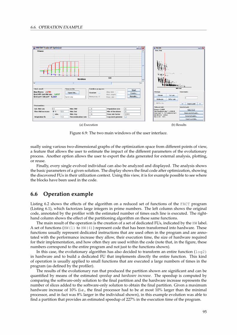
6.6. OPERATION EXAMPLE

(a) Execution (b) Results

Figure 6.9: The two main windows of the user interface.

sually using various two-dimensional graphs of the optimization space from different points of view,a feature that allows the user to estimate the impact of the different parameters of the evolutionaryprocess. Another option allows the user to export the data generated for external analysis, plotting,or reuse.

Finally, every single evolved individual can also be analyzed and displayed. The analysis showsthe basic parameters of a given solution. The display shows the final code after optimization, showingthe discovered FUs in their utilization context. Using this view, it is for example possible to see wherethe blocks have been used in the code.

6.6 Operation example

Listing 6.2 shows the effects of the algorithm on a reduced set of functions of the FACT program(Listing 6.1), which factorizes large integers in prime numbers. The left column shows the originalcode, annotated by the profiler with the estimated number of times each line is executed. The right-hand column shows the effect of the partitioning algorithm on these same functions.

The main result of the operation is the creation of a set of dedicated FUs, indicated by the HW label.A set of functions (HW(1) to HW(4)) represent code that has been transformed into hardware. Thesefunctions usually represent dedicated instructions that are used often in the program and are anno-tated with the performance increase they allow, their execution time, the size of hardware requiredfor their implementation, and how often they are used within the code (note that, in the figure, thesenumbers correspond to the entire program and not just to the functions shown).

In this case, the evolutionary algorithm has also decided to transform an entire function (log2)in hardware and to build a dedicated FU that implements directly the entire function. This kindof operation is usually applied to small functions that are executed a large numbers of times in theprogram (as defined by the profiler).

The results of the evolutionary run that produced the partition shown are significant and can bequantified by means of the estimated speedup and hardware increase. The speedup is computed bycomparing the software-only solution to the final partition and the hardware increase represents thenumber of slices added to the software-only solution to obtain the final partition. Given a maximumhardware increase of 10% (i.e., the final processor had to be at most 10% larger than the minimalprocessor, and in fact was 8% larger in the individual shown), in this example evolution was able tofind a partition that provides an estimated speedup of 227% in the execution time of the program.

95

CHAPTER 6. PROCESSOR EVOLUTION

function isPrime(u) { #28211if(u == 2) {#28211return true; #5000

}max = bin_sqrt(u); #28211

if(u % 2 != 0 && u > 2) { #23211for(i = 3; i < max; i + 2) { #105795if((u % i) == 0) { #95302return false; #7719

}}return true; #10493

}return false; #4999

}

function log2(u) { #164924x = 0; #164924

while(u != 0) { #1168952u = u >> 1; #1004028x = x + 1; #1004028

}return x; #164924

}

function isSquare(u) { #94777low = 0; #94777high = 0; #94777x = 0; #94777

if(u == 1) { #94777return true; #12315

}

low = (log2(u) >> 1) - 1; #82462high = (log2(u) >> 1) + 1; #82462low = pow(2, low); #82462high = pow(2, high); #82462

while(true) { #360086x = (low + high) >> 1; #360086

if(low > high) { #360086return false; #69115

}

if((x * x) < u) { #290971low = x + 1; #129104

}else{if((x*x) > u) { #161867high = x - 1; #148520

}else {return true; #13347

}}}}

Listing 6.1: Original code.

function isPrime (u) {HW(1)HW(3)if (u % 2 != 0 & u > 2) {

for (i = 3;i < max;i + 2) (9.5302) {if (u % i == 0){

return 0;}

}return 1;}

return 0;}

[HW] [HW] - function log2 (u) {x = 0;while (u != 0) (100.4028) {

u = u >> 1;x = x + 1;

}return x;}

function isSquare (u){low = 0;high = 0;x = 0;HW(1)low = log2(u) >> 1 - 1;high = log2(u) >> 1 + 1;low = pow(2, low);high = pow(2, high);while (1) (36.0086) {

x = low + high >> 1;HW(4)if (x * x < u) {

low = HW(2);}else {

if (x * x > u){high = x - 1;

}else{

return 1;}

}}

}

/∗∗∗∗∗∗∗∗∗∗∗∗∗∗∗∗∗∗∗∗∗∗∗/// Block HW(1) (Performance gain : 1.0002143413697018)// (Exec time : 20.0, HW Size : 49.0) − HW Bloc used 3 timesif (v == 0){return 1;

}

// Block HW(2) (Performance gain : 0.997791210375102)// (Exec time : 2.0, HW Size : 38.0) − HW Bloc used 4 timesi + 1

// Block HW(3) (Performance gain : 1.824315957433441)// (Exec time : 44.0, HW Size : 329.0) − HW Bloc used 3 timesmax = bin_sqrt(u);

// HW(4) (Performance gain : 1.0013923806061944)// (Exec time : 81.0, HW Size : 72.0) − HW Bloc used 1 timesif (low > high){

return 0;}/∗∗∗∗∗∗∗∗∗∗∗∗∗∗∗∗∗∗∗∗∗∗∗/

Listing 6.2: Sample result of partitioning.

96

6.7. EXPERIMENTAL RESULTS

6.7 Experimental results

To show the efficiency of our partitioning method, we tested it on two benchmark programs andseveral randomly-generated ones. The size of the applications tested lies between 60 lines of codefor the DCT program, which is an integer direct cosine transform, and 300 lines of code for the FACTprogram, which factorizes large integer in prime numbers. The last kind of programs tested arerandom generated programs with different genome sizes. The quality of our results can be quantifiedby means of the estimated speedup and hardware increase. The speedup is computed by comparingthe software-only solution to the final partition and the hardware increase represents the number ofslices in the VIRTEXTM II-3000 that have to be added to the software-only solution to obtain the finalpartition.

Figure 6.10: Exploration during the evolution (dynamic fitness function).

Figure 6.10 depicts the evolution, using 40 iterations per level, of 30 individuals for the FACT pro-gram using the dynamic fitness function. A maximum hardware increase of 20% has been specified.We can see that the exploration space is well covered during evolution. Figure 6.11 shows the cover-age of the fitness landscape during evolution for both fitness functions along with the best individualtrace for the same program.

Table 6.1 sums up the experiments that have been conducted to test our algorithm using bothfitness functions. Each figure in the table represents the mean of 500 runs. It is particularly interestingto note that all the results were obtained in the order of a few seconds and not minutes or hours as itis usually the case when GAs are involved. Despite that short running time, the algorithm convergedto very efficient solutions during that time.

Unfortunately, even if the domain is a rich source of literature, a direct comparison of our ap-proach to others seems very difficult. Indeed, the large differences that exist in the various designenvironments and the lack of common benchmarking techniques (which can be explained to the dif-ferent inputs of HW/SW partitioners) have already been identified in [López-Vallejo 03] to be a majordifficulty against direct comparisons.

97

CHAPTER 6. PROCESSOR EVOLUTION

Program name Gene Max HW incr. Est. HW. incr. Estimated Run time[bits] [slices] [slices] speedup [ms]

FACT 571∞ 65.17 % 4.41 3447

20 % 19.75 % 3.00 375010 % 9.66 % 2.38 3864

DCT 212 ∞ 71.37 % 2.77 547RND100 100 ∞ 1.4 % 1.23 250RND200 200 ∞ 1.0 % 1.08 734

(a) Static fitness

Program name Gene Max HW incr. Est. HW. incr. Estimated Run time[bits] [slices] [slices] speedup [ms]

FACT 571∞ 213 % 5.69 3250

20 % 19.92 % 2.92 282110 % 9.87 % 1.81 4100

DCT 212 ∞ 73.73 % 2.77 547RND100 100 ∞ 1.4 % 1.23 250RND200 200 ∞ 1.0 % 1.08 734

(b) Dynamic fitness

Table 6.1: Evolution results on various programs (mean value of 500 runs).

(a) Static function (b) Dynamic function

Figure 6.11: Best individual trace along with the explored fitness landscape.

98

6.8. CONCLUSION AND FUTURE WORK

6.8 Conclusion and future work

In this chapter we described an implementation of a new partitioning method using an hybrid GA thatis able to solve relatively large and constrained problems in a very limited amount of time. When con-sidered in the context of our automated software suite for bio-inspired systems generation, this workcan be used to automatically generate ad hoc functional units that can be used for the development ofontogenetic processors.

Albeit our method is tailored for the specific kind of processor architecture we are using in thisthesis, it remains general and could be used for almost every embedded system architecture with onlyminor changes.

The use of a dynamically-weighted fitness function introduced additional flexibility in the GA andpermitted to closely meet the constraints whilst maintaining an interesting performance. By usingseveral optimization passes, we reduced the search space and made it manageable by a GA. More-over, the granularity of the partitioning is determined dynamically rather than fixed before executionthanks to hierarchical clustering. The different levels determined by this technique thus representproblems of growing complexity that can be handled incrementally by the algorithm.

The results presented here, as well as those of others groups who have shown that HW/SW parti-tioning can be successfully used for FPGA soft-cores [Lysecky 05], are encouraging for future researchthat will address the unresolved issues of our system: for example, although the language in whichthe problem has to be specified remains simple, the method should be applied to well-known bench-marking suites to validate it more thoroughly. Another idea would be to work not on C code directlybut to take advantage of an intermediate representation presenting more regularity, such as GIMPLE(discussed in section 4.2).

Future work within this topic calls for two main axes of research. On one hand it would be inter-esting to introduce energy as a parameter for the fitness function in order to optimize the power con-sumption of the desired embedded circuit. On the other hand, it would also be interesting to explorethe possibility of automatically generating the HDL code corresponding to the extracted hardwareblocks, a tool that would allow us to verify our approach on a larger set of problems and also on realhardware. Another solution would be to use direct C to HDL translation based on languages such asHandel-C [Chappell 02] or Impulse C6 [Pellerin 05].

6http://www.impulsec.com

99

Bibliography

[Ahmed 04] Usman Ahmed & Gul N. Khan. Embedded system partitioning with flexible granularityby using a variant of tabu search. In Proceedings of the Canadian Conference onElectrical and Computer Engineering, vol. 4, pages 2073–2076, May 2004.

[Catania 97] Vincenzo Catania, Michele Malgeri & Marco Russo. Applying Fuzzy Logic to Code-sign Partitioning. IEEE Micro, vol. 17, no. 3, pages 62–70, 1997.

[Chappell 02] Stephen Chappell & Chris Sullivan. Handel-C for Co-Processing and Co-Design ofField Programmable System on Chip. In Proceedings of the Jornadas sobre Com-putación Reconfigurable y Aplicaciones (JCRA02), pages 65–70, 2002.

[Dick 98] Robert P. Dick & Niraj K. Jha. MOGAC: a multiobjective genetic algorithm forhardware-software cosynthesis of distributed embedded systems. IEEE Transactions onComputer-Aided Design of Integrated Circuits and Systems, vol. 17, no. 10, pages920–935, October 1998.

[Eles 97] Petru Eles, Krysztof Kuchcinski, Zebo Peng & Alexa Doboli. System Level Hard-ware/Software Partioning Based on Simulated Annealing and Tabu Search. Design Au-tomation for Embedded Systems, vol. 2, pages 5–32, 1997.

[Ernst 93] Rolf Ernst, Jörg Henkel & Thomas Benner. Hardware-Software Cosynthesis for Micro-controllers. In IEEE Design & Test of Computers, pages 64–75, December 1993.

[Ernst 02] Rolf Ernst, Jörg Henkel & Thomas Benner. Readings in Hardware/Software Co-Design,chapter Hardware-software cosynthesis for microcontrollers, pages 18–29. KluwerAcademic Publishers, 2002.

[Gupta 92] Rajesh K. Gupta & Giovanni de Micheli. System-level Synthesis using Re-programmable Components. In Proceedings of the European Design AutomationConference (EDAC), pages 2–7, August 1992.

[Harkin 01] J. Harkin, T. M. McGinnity & L.P. Maguire. Genetic algorithm driven hardware-software partitioning for dynamically reconfigurable embedded systems. Microproces-sors and Microsystems, vol. 25, no. 5, pages 263–274, August 2001.

[Henkel 98] Jörg Henkel & Rolf Ernst. High-Level Estimation Techniques for Usage in Hardware/-Software Co-Design. In Asia and South Pacific Design Automation Conference,pages 353–360, 1998.

[Henkel 01] Jörg Henkel & Rolf Ernst. An Approach to Automated Hardware/Software PartitioningUsing a Flexible Granularity that is Driven by High-Level Estimation Techniques. IEEETransactions on Very Large Scale Integration (VLSI) Systems, vol. 9, no. 2, pages273–289, April 2001.

[Hou 96] Junwei Hou & Wayne Wolf. Process Partitioning for Distributed Embedded Systems. InProceedings of the 4th International Workshop on Hardware/Software Co-Design(CODES’96), page 70, Washington, USA, 1996. IEEE Computer Society.

101

BIBLIOGRAPHY

[Koza 92] John R. Koza. Genetic Programming: On the Programming of Computers by Means ofNatural Selection. MIT Press, 1992.

[López-Vallejo 03] Marisa López-Vallejo & Juan Carlos López. On the Hardware-Software PartitioningProblem: System Modeling and Partitioning Techniques. ACM Transactions on DesignAutomation of Electronic Systems, vol. 8, no. 3, July 2003.

[Lysecky 05] Roman Lysecky & Frank Vahid. A Study of the Speedups and Competitiveness of FPGASoft Processor Cores using Dynamic Hardware/Software Partitioning. In Proceedings ofthe conference on Design, automation and test in Europe (DATE’05), pages 18–23,Washington, USA, 2005. IEEE Computer Society.

[Oudghiri 92] H. Oudghiri & B. Kaminska. Global weighted scheduling and allocation algorithms. InProceedings of the European Conference on Design Automation (DATE’92), pages491–495, March 1992.

[Pellerin 05] David Pellerin & Edward A. Thibault. Practical FPGA Programming in C. PrenticeHall, 2005.

[Pitkänen 05] Teemu Pitkänen, Tommi Rantanen, Andrea G. M. Cilio & Jarmo Takala. HardwareCost Estimation for Application-Specific Processor Design. In Embedded ComputerSystems: Architectures, Modeling, and Simulation, vol. 3553 of Lecture Notes inComputer Science, pages 212–221. Springer Berlin / Heidelberg, 2005.

[Renders 94] J.-M. Renders & H. Bersini. Hybridizing genetic algorithms with hill-climbing methodsfor global optimization: two possible ways. In Proceedings of the First IEEE Conferenceon Evolutionary Computation, vol. 1, pages 312–317, June 1994.

[Srinivasan 98] V. Srinivasan, S. Radhakrishnan & R. Vemuri. Hardware/software partitioning withintegrated hardware design space exploration. In Proceedings of the conference onDesign, automation and test in Europe (DATE’98), pages 28–35, Washington, USA,1998. IEEE Computer Society.

[Vahid 94] Frank Vahid, Daniel D. Gajski & Jie Gong. A binary-constraint search algorithm forminimizing hardware during hardware/software partitioning. In Proceedings of theconference on European design automation (EURO-DAC’94), pages 214–219, 1994.

[Vahid 95] Frank Vahid & Daniel D. Gajski. Incremental Hardware Estimation During Hardware/-Software Functional Partitioning. IEEE Transactions on VLSI Systems, vol. 3, no. 3,pages 459–464, September 1995.

[Wiangtong 02] Theerayod Wiangtong, Peter Y.K. Cheung & Wayne Luk. Comparing Three HeuristicSearch Methods for Functional Partitioning in Hardware-Software Codesign. DesignAutomation for Embedded Systems, vol. 6, no. 4, pages 425–449, July 2002.

[Wiangtong 04] Theerayod Wiangtong. Hardware/Software Partitioning And Scheduling For Reconfig-urable Systems. PhD thesis, Imperial College London, February 2004.

102

Part II

Networks of processing elements

103

Chapter 7

The CONFETTI platform

“The time has come,”the Walrus said,

“to talk of many things.”

LEWIS CARROLL, The Walrus and The Carpenter

7.1 Introduction and motivations

AKEY ASPECT of the research that was pursued, first in the Logic Systems Laboratory (LSL) ledby Professor Daniel Mange and then in the Cellular Architectures Research Group (CARG), has

tried to approach cellular computing by designing large arrays of custom processing elements andby analyzing how some of the mechanisms involved in the development of biological organisms canbe effectively applied to these arrays in order to achieve useful properties such as fault tolerance orgrowth.

Our work represents the continuation of this research, which has traditionally relied on the hard-ware realization of prototype systems in order to experimentally verify their properties and to analyzetheir efficiency. Considering the complexity of this kind of systems, their prototyping in hardware re-quires vast amounts of reconfigurable resources and has led us to the realization of a custom platformspecifically designed to implement and test complex cellular computing arrays. In this chapter, wepresent the salient features of this platform, which we have labeled CONFETTI, for CONFigurable Elec-Tronic TIssue. More precisely, we will present a hardware platform that is able to support the necessarynetworking and computing elements that can then form what we call a scalable Network Of Chips.

The chapter is organized as follows: in the next section, we will give a brief overview of thecomputational approach that motivated the hardware architecture and describe the state of the art inthe domain by analyzing some previous work. The hardware platform itself will then be describedin some detail in section 7.3 before discussing several general issues, such as power consumptionand integrated test and monitoring, in section 7.4. Finally, section 7.5 concludes this chapter andintroduces future work.

Preliminary remark The large majority of the hardware implementations presented in this chapter – be theyschematics or PCBs – was realized by Fabien Vannel in the context of his PhD thesis [Vannel 07], even thoughwe participated in the design and routing of some of the PCBs. On the “middleware side”, i.e. the VHDLcoding of the FPGA, we reused in this project only the code that Dr. Vannel wrote to drive the RGB screen andreconfigure the cell FPGA from the routing layer (see section 7.3.5). Beside that, every software and hardwarecomponent described in this work is our personal contribution.

105

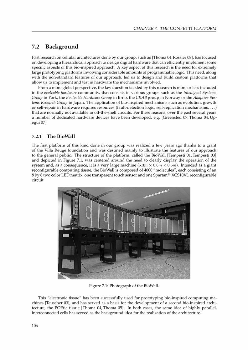
CHAPTER 7. THE CONFETTI PLATFORM

7.2 Background

Past research on cellular architectures done by our group, such as [Thoma 04,Rossier 08], has focusedon developing a hierarchical approach to design digital hardware that can efficiently implement somespecific aspects of this bio-inspired approach. A key aspect of this research is the need for extremelylarge prototyping platforms involving considerable amounts of programmable logic. This need, alongwith the non-standard features of our approach, led us to design and build custom platforms thatallow us to implement and test in hardware the mechanisms involved.

From a more global perspective, the key question tackled by this research is more or less includedin the evolvable hardware community, that consists in various groups such as the Intelligent SystemsGroup in York, the Evolvable Hardware Group in Brno, the CRAB group in Norway or the Adaptive Sys-tems Research Group in Japan. The application of bio-inspired mechanisms such as evolution, growthor self-repair in hardware requires resources (fault-detection logic, self-replication mechanisms, . . . )that are normally not available in off-the-shelf circuits. For these reasons, over the past several yearsa number of dedicated hardware devices have been developed, e.g. [Greensted 07, Thoma 04, Up-egui 07].

7.2.1 The BioWall

The first platform of this kind done in our group was realized a few years ago thanks to a grantof the Villa Reuge foundation and was destined mainly to illustrate the features of our approachto the general public. The structure of the platform, called the BioWall [Tempesti 01, Tempesti 03]and depicted in Figure 7.1, was centered around the need to clearly display the operation of thesystem and, as a consequence, it is a very large machine (5.3m × 0.6m × 0.5m). Intended as a giantreconfigurable computing tissue, the BioWall is composed of 4000 “molecules”, each consisting of an8 by 8 two color LED matrix, one transparent touch sensor and one Spartanr XCS10XL reconfigurablecircuit.

Figure 7.1: Photograph of the BioWall.

This “electronic tissue” has been successfully used for prototyping bio-inspired computing ma-chines [Teuscher 03], and has served as a basis for the development of a second bio-inspired archi-tecture, the POEtic tissue [Thoma 04, Thoma 05]. In both cases, the same idea of highly parallel,interconnected cells has served as the background idea for the realization of the architecture.

106

7.3. THE CONFETTI EXPERIMENTATION PLATFORM

Despite the fact that the BioWall has fulfilled its role and has been successfully used during severalyears, it suffers from several limitations which hinder the development of new applications. Theselimitations are related to the FPGA used, the clock distribution, the autonomy of the system and thedisplay (see for more details [Vannel 07, p. 106]):

• The limitations of the FPGA used in the BioWall are twofold. First, the FPGA model chosenat the time of its conception had to offer good performance at a low price. For these reasons,Spartan XCS10XL were selected. In comparison to what is available on the market today, theperformance of these chips is quite limited.

The second limitation comes from the FPGA configurations. In fact, every FPGA in the BioWallhas to use the same configuration, which limits the functionality of every unit to the 10000equivalent logic gates of the Spartan XCS10XL.

• A a single clock source is used for the whole system. Consequently, the considerable delaysinherent in propagating a global signal over distances measured in meters limit the clock speedto about 1 MHz. This fact confines the system to applications where the required computationalspeed is very low, such as those in which human interaction is required (the intended target ofthe platform).

• The entire system is controlled by an electronic board connected to a PC and aimed at configur-ing all the FPGAs and distributing the clock signal to the 4000 FPGAs. Thus, the BioWall acts asa slave electronic system even if the application does not require any interaction with the hostcomputer once configured. This limitation prevents the BioWall from being fully autonomousand introduces a functional bottleneck at the interface between the PC and the reconfigurablelogic.

• The huge display of the BioWall is only able to display three different colors because it is com-posed of red and green LEDs. Furthermore, as the LEDs’ intensity can not be changed, there isno brightness control and intermediate shades are not available.

• Each FPGA can communicate only with its direct neighbors and no routing mechanism is present.We will discuss this limitation further in chapter 8.

These drawbacks, along with the evolution of programmable logic devices, have led us to definea novel platform for the implementation of our systems. In the next sections, we will present thestructure of the new platform and its salient features.

7.3 The CONFETTI experimentation platform

This novel hardware platform is aimed at the realization of cellular architectures. The system is builthierarchically from a simple computing unit, called the cell, which is based on an FPGA and SRAMmemory. Several of these units can then be connected, using a high-speed serial communication pro-tocol, to a more complex structure (a stack) consisting of four different kinds of interconnected boards(computational, routing, power supply, and display). These stacks can then be joined together to forman arbitrarily large parallel network of programmable circuits. This structure, while theoretically uni-versal in its operation, is however particularly suited for the implementation of cellular computing,as we will see.

The platform consists of a scalable array of homogeneous processing nodes physically arrangedas a networked computing mesh. It is mainly characterized by its flexibility, obtained through a dual-layered arrangement of FPGAs, with a layer dedicated to processing and the other to networking.

This strict separation of computing and networking resources enables independent experimenta-tion of new algorithms in both domains as well as at their interface.

As we will see, the platform tries to avoid the BioWall’s shortcomings by proposing an increasedamount of versatility and interchangeability in the different constituting elements of the hardwaresystem. Moreover, the system is built hierarchically by connecting elements of increasing complexitywhich permits to handle more easily the intricacy of the whole system.

107

CHAPTER 7. THE CONFETTI PLATFORM

7.3.1 Overview – A hierarchical construction

The platform is composed of a set of stacks of printed-circuit boards (PCBs) (Figure 7.2), which can beconnected together side by side. Connecting several stacks together potentially allows the creation ofan arbitrarily large surface of programmable logic that is used, in this present work, as a network ofCPUs where all components can be reconfigured.

Routing

Cell boards

Power

Display

(a) Schematic (b) Photograph

Figure 7.2: A stack schematic and photograph.

Each of these stacks is composed of four kinds of boards:

1. The cell boardsUp to 18 of these boards can be used per stack. They represent the computational part of thesystem and are composed of an FPGA and an 8 Mbit static memory. Each board is directlyplugged, via a connector, into a corresponding routing FPGA in the subjacent routing board.

2. The routing boardThis board constitutes the communication layer of the system. Articulated around 18 FPGAs ina mesh topology, the board can implement different routing algorithms to form a network thatprovides inter-FPGA communication but also communication to other routing boards.

3. The display boardThe topmost layer of the stack is composed of a display board that consists of a RGB matrix LEDdisplay to which a touch sensitive surface has been added.

4. Power supply boardAbove the routing layer lies a board that generates all the power supplies required by the systemand handles functions such as startup and monitoring.

This hardware structure proposes an increased amount of versatility compared to other platforms,notably because its modular organization allows interchanging all the elements of the system. If thismight be interesting in the perspective of debugging and replacing faulty parts, the clear advantage ofthis approach resides in the fact that the computing elements, which are plugged into the system andnot soldered on it, could also be easily replaced. This latter option is of particular interest in the largerperspective of a prototyping board for unconventional computing: nothing prevents the replacementof the current cells with more “exotic” or non-standard units that could potentially be of interest forresearch in bio-inspired mechanisms.

108

7.3. THE CONFETTI EXPERIMENTATION PLATFORM

(a) SRAM chips, FPGA and connector to routing layer

Touch sensor

RGB LED Display

Cell boardfor computation

Routing layer

High-speed link

ConnectorData link

(b) Cell board schematic overview

Figure 7.3: Pictures and schematic of the cell board.

7.3.2 The cell board

This small PCB, depicted in Figure 7.3a, constitutes the basic building block of our hardware platform.It is articulated around a SPARTANr 3 FPGA1 from Xilinxr coupled with 8 Mbit of 10 ns SRAMmemory and a temperature measurement chip. Equivalent to 200′000 logic gates, the core of thisboard possesses some interesting features such as hardware multipliers, 18 kbit of internal dual-portmemory and four digital clock managers (DCM) that allow to obtain, from the 50 MHz local clock,working frequencies up to 300 MHz. All these components are soldered on a very small (26× 26 mm)eight-layer PCB.

The board contains various connections to the others components of the system that all passthrough the connector visible on top of Figure 7.3a and Figure 7.3b. The connectivity of the boardis as follows:

Type Number of lines Description

High-speed bus 6 LVDS Differential high-speed communication with the subjacentFPGA on the routing level (3 pairs in each direction),500 Mbit max. per pair.

Low-speed bus 6 Communication bus to the routing FPGA that carries the dis-play and control signals.

Configuration 5 Used to configure the FPGA via the routing board. The bit-stream is sent serially.

Clock 1 50 MHz clock shared with the underlying routing FPGA.Reset 1 Reset signal generated by the underlying routing FPGA.Temperature 3 Digital temperature readout.Power 12 Carries the power supply of the FPGA and SRAM modules.

Table 7.1: Cell board I/O signals.

The FPGA allows any soft-core CPU to be instantiated as a computing node. In this work how-ever, we will focus only on the use of the ULYSSE processor. In the context of this platform, thecustomization ability of the processor will help to develop an ad-hoc network interface with DMAwith the capability to modify the processor’s code at run-time using specially-formed data packets(see section 8.4.1).

1The exact model is the XC3S200 FPGA.

109

CHAPTER 7. THE CONFETTI PLATFORM

As seen from this board, ULYSSE has access to the touch sensor area above it and to an 8 by 8slice of the RGB display (Figure 7.3b). The information is passed not via a direct connections to theseelements but thanks to a low speed communication bus with the routing board, which is described inthe next section.

7.3.3 The routing board

(a) Top view – The mesh grid arrangement of the FPGAsis clearly visible. Four cells have been inserted in top-leftcorner of the board.

(b) Bottom view – The 50 MHz oscillators are visible alongwith the inter-board connectors.

Figure 7.4: Routing board pictures.

One of the main challenges in today’s hardware architectures resides in implementing versatilecommunication capabilities that are able to provide a sufficient bandwidth whilst remaining cost- andsize-efficient, as evidenced in research on NoC [Bjerregaard 06] and other systems [Moraes 04]. Thisaspect of parallel systems is unfortunately often ignored in bio-inspired hardware approaches and isanother factor that prevent the implementation of complex applications. In our case, the addition ofa network layer enables data to be moved not just within the various FUs of the processor but alsooutside of it to realize a complex Network Of Chips of virtually unlimited size.

To accomplish this, the functions of computation and communication were logically and physi-cally split. With this separation, we were able to preserve the whole of the computational resources ofthe cell board while retaining full flexibility for the communication network in our system within therouting board, which also handles tasks such as system configuration and display management. As itconstitutes a subject in itself, routing and communications will be discussed in the next chapter (section8.3, page 121) and we will only describe here the hardware structure of the routing board.

Measuring 192mm× 96mm, this highly complex board (twelve layers) has components solderedon both sides and can host as many as eighteen cell boards. Based on a six-by-three regular gridtopology (Figure 7.5), this board is composed of a set of 18 reconfigurable FPGA circuits and 18 Flashmemories.

Connectivity

Each of these routing FPGAs is connected to its neighbors with high-speed low-voltage differentialsignalling (LVDS) lines. As the routing boards constitute the communicating backplane of the wholeCONFETTI, connections between the different stacks are also implemented here. External connectorsare present on the four sides of the board and provide the same connectivity as the links betweenthe FPGAs: two adjacent routing boards then represent effectively a single uniform surface of FPGAs.The modularity of the setup allows the creation of systems consisting of several stacks that behave asa single, larger stack.

Configuration of the FPGAs

In parallel to these very high speed links that are used for communication, another bus, working at50 MHz, is also present on the routing layer. This bus, as we will see now, is used for transmitting,

110

7.3. THE CONFETTI EXPERIMENTATION PLATFORM

50MHz

Cellconnector

Spartan 3XCS200

C° sensor

Flash

To powerand display

Figure 7.5: Routing board schematic.

loading and storing different cell configurations.The various reconfigurable circuits used in CONFETTI are all based on SRAM technology, which

means they can be reconfigured an unlimited amount of times and that the configuration requires arelatively short time (typically 20 ms). The routing FPGAs all share the same configuration bitstream,stored in a memory which can be accessed via a JTAG connector on the routing board, i.e. all therouting FPGAs implement the same circuit. The situation is more complex for the FPGAs on the cellboards: as they could have a different configuration and even be reconfigured dynamically, one of theproblems that need to be addressed by the system is how to convey the correct configuration to eachof the cell FPGAs.

This task is performed within the routing board: each routing FPGA can access an adjacent 16 MbitFlash memory, which can be used to store as many as sixteen different configurations for the cellFPGAs or serve as non-volatile memory available for applications.

The contents of this memory can be modified using an external interface connected to a computer(more on this in section 7.4.3). At the moment, this constitutes the only way to store new applicationsbitstreams to be executed by the cells. Of course, the configurability of the routing FPGAs enablesalmost unlimited versatility in the configuration scheme, allowing for example the implementationof applications that would update the Flash contents using external memories or retrieve the cellconfigurations from sources other than the local Flash memory, such as LAN or WiFi connections.

7.3.4 The power supply board

The SPARTANr 3 FPGAs that are used throughout the CONFETTI system are built on a 90 nm CMOSprocess. This gives them the advantage of being very fast and of having lots of embedded features butalso has the disadvantage of needing several low-power voltages. Thus, the FPGA core is powered bya 1.2 V voltage but also needs 2.5 V for the LVDS interface and for configuration purposes. Finally, a3.3 V voltage is needed to interface with the Flash and SRAM memories. Moreover, all these voltagesneed to be well stabilized, as Xilinxr FPGAs allow only ±5 % tolerance.

To cope with all these requirements and the fact that the eighteen cells and the routing board arenot only very complex but also power-hungry, a dedicated power supply board was added. This six-layer PCB, mainly responsible of supplying the correct voltage to all the components on the boardsunderneath, has the same size as the routing board. Articulated around six DC / DC converter, thisboard generates from a global 5 V the three mentioned voltages of 1.2 V, 2.5 V and 3.3 V that arethen brought, using six 8-pins connectors, to the routing board where they are used to power-up the

111

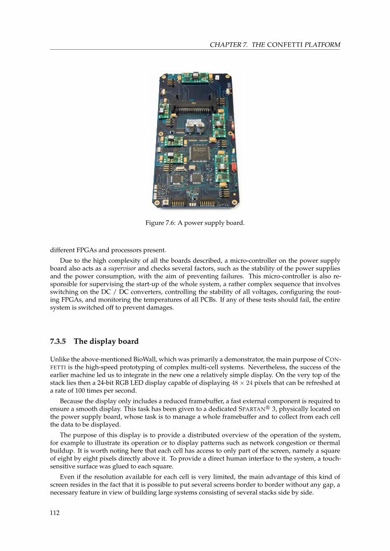
CHAPTER 7. THE CONFETTI PLATFORM

Figure 7.6: A power supply board.

different FPGAs and processors present.

Due to the high complexity of all the boards described, a micro-controller on the power supplyboard also acts as a supervisor and checks several factors, such as the stability of the power suppliesand the power consumption, with the aim of preventing failures. This micro-controller is also re-sponsible for supervising the start-up of the whole system, a rather complex sequence that involvesswitching on the DC / DC converters, controlling the stability of all voltages, configuring the rout-ing FPGAs, and monitoring the temperatures of all PCBs. If any of these tests should fail, the entiresystem is switched off to prevent damages.

7.3.5 The display board

Unlike the above-mentioned BioWall, which was primarily a demonstrator, the main purpose of CON-FETTI is the high-speed prototyping of complex multi-cell systems. Nevertheless, the success of theearlier machine led us to integrate in the new one a relatively simple display. On the very top of thestack lies then a 24-bit RGB LED display capable of displaying 48× 24 pixels that can be refreshed ata rate of 100 times per second.

Because the display only includes a reduced framebuffer, a fast external component is required toensure a smooth display. This task has been given to a dedicated SPARTANr 3, physically located onthe power supply board, whose task is to manage a whole framebuffer and to collect from each cellthe data to be displayed.

The purpose of this display is to provide a distributed overview of the operation of the system,for example to illustrate its operation or to display patterns such as network congestion or thermalbuildup. It is worth noting here that each cell has access to only part of the screen, namely a squareof eight by eight pixels directly above it. To provide a direct human interface to the system, a touch-sensitive surface was glued to each square.

Even if the resolution available for each cell is very limited, the main advantage of this kind ofscreen resides in the fact that it is possible to put several screens border to border without any gap, anecessary feature in view of building large systems consisting of several stacks side by side.

112

7.4. THE CONFETTI SYSTEM

7.4 The CONFETTI system

The previous section has been devoted to the description of a complete basic element: the stack. Aswe mentioned earlier, a complete CONFETTI system consists of an arbitrary number of such stacksseamlessly joined together (through the border connectors in the routing board) in a two-dimensionalarray.

The current test configuration that has been built and tested, for example, consists of six stacks ina 3 by 2 array, as shown in Figure 7.7. The same figure also depicts a different layout of the boardswhere a 2 by 3 array is used. One can also note the presence of a metallic frame to provide a rigidstructure that ensures good connections between the different stacks.

2

1. Stack2. Mechanical support3. Fan board4. Interconnect board

3 4

3

1

(a) Layout 1

1. Mechanical frame2. Fans3. East / West interconnect4. North / South interconnect5. Stack

34

2

2

1

5

(b) Layout 2

Figure 7.7: The CONFETTI system in two different configurations.

The connection of several boards together potentially allows the creation of arbitrarily large sur-faces of programmable logic. However, considerations of power consumption, thermal management,and system monitoring come into play for a system of this kind.

7.4.1 Power consumption considerations

The power consumption of the system is very difficult to determine in advance with a reconfigurablesystem, since it heavily depends on the FPGA configuration, and will change with each application.However, Xilinxr XPowerr2 tools give a worst-case current consumption of 1 A per core. This esti-mation is based on XC3S200-VT100-4 FPGA with a clock frequency of 100 MHz and full utilization ofthe FPGA resources.

As we have a total of thirty-six of these FPGAs for each stack, the maximum current that mightbe drained could be as high as 36 A on the 1.2 V power supply. In comparison, the power estimationfor 2.5 V and 3.3 V are very low, with only 4 A for each. In addition to the FPGAs, the last significantenergy consumer is constituted by screen that can use a maximum of 30 W. Thus, the total maximumconsumption for one stack is 100 W, provided by an external 5 V regulated power supply to the powerboard.

7.4.2 Thermal management

Despite the fact that the reconfigurable circuits in the platform use a state-of-the-art fabrication tech-nology that makes them less power hungry than previous generation FPGAs, the number of circuitsinvolved in the whole system makes thermal management a real issue, each stack consuming a maxi-mum total of 100 W. To solve it, we had to implement an adequate cooling system in order to evacuatethe generated heat. Thus, we integrated boards with fans on the top and bottom borders of the whole

2See [Xil 07] and http://www.xilinx.com/products/design_resources/power_central/index.htm

113

CHAPTER 7. THE CONFETTI PLATFORM

system. Two different types of fan boards have been used: on the bottom, fans are used for introduc-ing cooler air on the FPGAs and on the top, fans extract the hot air away from the boards. Each boardcontains between six and height fans, each independently controllable.

To ensure a good thermal protection without having to turn on all the available fans, the tempera-ture of several components is constantly monitored on:

• every cell;

• every FPGA on the routing board but also three additional locations on the board;

• every power supply board, with six temperature sensors.

It is then relatively easy to detect thermal hot spots and turn on the necessary fans, a process whichis done by a dedicated component described in the next section.

7.4.3 Integrated test and monitoring

Because of the relatively high price of the components and the low number of stacks produced, wetook precautions to minimize the risks of component failure due to short circuits or thermal stress.

LCD Display To power suppliesand fan boards

PIC uController

Mercuryinterface

High-speeddi�erential lines

MicroblazeCPU

OPB

UART

PIC uController

UART

USBinterface

CypressUSB FIFO

OPB

CAN BusParallel bus

Serial link Serial link

Embeddedmemory

Spartan 3-XCS200

Host PC To CONFETTI

Con�gbus

MonitorbusTimer Interrupt

controller

Figure 7.8: Schematic of the monitor and control board.

Thus, each power supply works in limited current mode, in which 20 A at 5 V can be sourced.Moreover, despite the fact that the whole system can be used in a configuration where it is completelyindependent of any external control mechanism, a supervisor board has been developed in order tomonitor the whole system but also to help debugging (Figure 7.8). This board, which lies next to theCONFETTI system, contains several elements:

• a SPARTANr 3 FPGA in which a MICROBLAZETM CPU has been instantiated;

• an USB interface chip for the MICROBLAZETM that allows the transmission of configurationsand data;

114

7.5. CONCLUSION AND FUTURE WORK

• a CAN protocol controller, managed by another micro-controller, which handles the differentpower supplies and fans of the system.

Thanks to the USB connection with an host PC, it becomes possible to monitor and control variousparameters related to the support of the CONFETTI platform. Figure 7.9 shows a control software toolthat was developed for this purpose and that allows to monitor and switch each power supply andfan individually and globally, to monitor the various temperature sensors, and to control differentelectrical parameters.

Figure 7.9: Remote control software of the monitoring tools.

7.5 Conclusion and future work

In this chapter, we described a novel hardware platform aimed at the realization of cellular computingapplications. The versatility of the platform along with its potential computational power offer veryinteresting perspectives not only for the exploration of various routing algorithms but also in termsof future developments.

For example, should more processing power be needed, the cell boards could easily be replacedby a bigger reconfigurable device or by a different kind of circuit. Similarly, the system’s modularityimplies that few changes would be required, for example, to allow different types of cell boards onthe same routing substrate.

Aside from the computational aspect, the system is also open to several improvements related toI/O. For example, it is clear that the current external USB connection is insufficient for high bandwidthapplications and an improvement to the system is the introduction of high-speed I/O boards that,placed on the borders of the array, could allow the implementation of data-intensive applications(video streaming, for example).

To exploit the features of the system, we will describe in the next chapter the necessary set of toolsfor routing data packets inside the CONFETTI platform. This done, we will then demonstrate howparallel applications can be implemented easily thanks to different software abstractions organizedin layers.

115

Bibliography

[Bjerregaard 06] Tobias Bjerregaard & Shankar Mahadevan. A survey of research and practices ofNetwork-on-chip. ACM Computing Survey, vol. 38, no. 1, page 1, 2006.

[Greensted 07] A.J. Greensted & A.M. Tyrrell. RISA: A Hardware Platform for Evolutionary Design. InProc. IEEE Workshop on Evolvable and Adaptive Hardware (WEAH07), pages 1–7,Honolulu, Hawaii, April 2007.

[Moraes 04] Fernando Moraes, Ney Calazans, Aline Mello, Leandro Möller & Luciano Ost. HER-MES: an infrastructure for low area overhead packet-switching networks on chip. IntegratedVLSI Journal, vol. 38, no. 1, pages 69–93, 2004.

[Rossier 08] Joël Rossier. Self-Replication of Complex Digital Circuits in Programmable Logic Devices.PhD thesis, École Polytechnique Fédérale de Lausanne, 2008.

[Tempesti 01] Gianluca Tempesti, Daniel Mange, André Stauffer & Christof Teuscher. The BioWall:an electronic tissue for prototyping bio-inspired systems. In Proceedings of the 3rd Nasa/-DoD Workshop on Evolvable Hardware, pages 185–192, Long Beach, California, July2001. IEEE Computer Society.

[Tempesti 03] Gianluca Tempesti & Christof Teuscher. Biology Goes Digital: An array of 5,700 SpartanFPGAs brings the BioWall to "life". XCell Journal, pages 40–45, Fall 2003.

[Teuscher 03] Christof Teuscher, Daniel Mange, André Stauffer & Gianluca Tempesti. Bio-InspiredComputing Tissues: Towards Machines that Evolve, Grow, and Learn. BioSystems, vol. 68,no. 2–3, pages 235–244, February–March 2003.

[Thoma 04] Yann Thoma, Gianluca Tempesti, Eduardo Sanchez & J.-M. Moreno Arostegui. PO-Etic: An Electronic Tissue for Bio-Inspired Cellular Applications. BioSystems, vol. 74,pages 191–200, August 2004.

[Thoma 05] Yann Thoma. Tissu Numérique Cellulaire à Routage et Configuration Dynamiques. PhDthesis, École Polytechnique Fédérale de Lausanne, 2005.

[Upegui 07] Andres Upegui, Yann Thoma, Eduardo Sanchez, Andres Perez-Uribe, Juan-Manuel Moreno Arostegui & Jordi Madrenas. The Perplexus bio-inspired reconfigurablecircuit. In Proceedings of the 2nd NASA/ESA Conference on Adaptive Hardwareand Systems (AHS07), pages 600–605, Washington, USA, 2007.

[Vannel 07] Fabien Vannel. Bio-inspired cellular machines: towards a new electronic paper architecture.PhD thesis, École Polytechnique Fédérale de Lausanne, Lausanne, 2007.

[Xil 07] Xilinx. Xilinx Power Estimator User Guide, 2007. http://www.xilinx.com/products/design_resources/power_central/ug440.pdf.

117

Chapter 8

CONFETTI communication andsoftware support

“Im Gebirge ist der nächste Weg von Gipfel zu Gipfel:aber dazu musst du lange Beine haben.”

“In the mountains the shortest route is from peak to peak,but for that you must have long legs.”

FRIEDRICH NIETZSCHE, Also sprach Zarathustra

WHEN WE described in the previous chapter the shortcomings of the BioWall, we deliberately didnot expand on what, in our opinion, constitutes the strongest limitation of the system: the lack

of adequate software support to program the platform and the impossibility to communicate fartherthan from the direct neighbor, which greatly limits the range of possible computations.

In this chapter, we will describe how we managed to remove both these constraints in CONFETTIby first implementing an efficient routing algorithm that provides powerful communication capabil-ities to the cells and then by developing a set of tools that attempt to tackle the software problem byproviding a simple but complete software framework to handle the complexity of the system.

8.1 Introduction and motivations

If CONFETTI makes available to the user an impressive amount of raw processing power, the majordifficulty of how to harvest this power remains unsolved. Considering that computing generallyrequires data to work on, this implies that without adequate and efficient means to bring these datato the processing nodes, the risk of underusing the resources due to an ill-designed communicationsystem is high. Moreover, using ULYSSE as a processing element implies the opportunity to considernetworking as a “natural extension” of the Move model in which the data are not displaced only insidea processor but also outside of it, extending the paradigm a step further.

With these elements in mind, we will first consider in this chapter the different possibilities offeredfor communicating. In the next section, we will first detail how local high-speed communication isachieved with the hardware implementation of physical links that provide inter-FPGA communica-tion. We will then explain how these short-distance links can be used in conjunction with a routingelement to provide long-distance point-to-point communication between the PEs. After that, section8.5 will be devoted to the software messaging layer that is built atop that hardware to provide efficientprimitives – such as broadcasting – that simplify the programming of networked applications but alsoacts as an extensible framework for distributed applications. With this software layer, it becomes pos-sible to quickly evaluate new algorithms, techniques and ideas in the field of bio-inspired computingbut also to harvest more easily the computing resources of hundreds of FPGAs. To demonstrate thislast idea, we will validate the whole hardware-software framework presented in this chapter with an

119

CHAPTER 8. CONFETTI COMMUNICATION AND SOFTWARE SUPPORT

application that shows how it can be used to develop a distributed cellular automaton and extendedto less regular computations.

8.2 High-speed communication links

The first step required to be able to transmit information among the different CPUs present in thecell boards is to create local communication between the FPGAs of the routing layer, a step that mustcope with a certain amount of constraints. First, the routing FPGAs possess only a limited numberof wires (6) that can be used to implement high-speed communications in every direction, labeledNorth-East-South-West and Local (connected to the cell board) (see Figure 8.1).

Using only these links, the question is how to communicate efficiently and in full-duplex, i.e. sothat both “sides” can communicate simultaneously, under the additional constraint that since scalabil-ity is a key feature of our architecture, no global clock is available to the system. This latter constraintimplies that synchronization between the different FPGAs is not straightforward, notably to transmitinformation.

The first solution we tried was an asynchronous approach. However, because transmission delayscan be relatively long in our system and only a few bits of parallel data can be used due to the limitednumber of wires, the use of a request-acknowledge pair in asynchronous transmission was too slow(early tests showed that the maximum bandwidth achievable using this technique was limited toabout 50 Mbit/s).

RoutingFPGA

RoutingFPGA

RoutingFPGA

RoutingFPGA

RoutingFPGA

RoutingFPGA

RoutingFPGA

RoutingFPGA

RoutingFPGA

CellFPGA

CellFPGA

CellFPGA

CellFPGA

CellFPGA

CellFPGA

CellFPGA

CellFPGA

CellFPGA

Mercurysender

Mercuryreceiver

rdy

dta

clk

rdy

dta

clk

Figure 8.1: MERCURY high-speed links.

Depicted in Figure 8.1 and Figure 8.2, the solution retained is based on two modules: the first as asender that transmits the clock along with serialized data to the second module that acts as a receiver.This receiver uses a dual-clock, dual-ported 32 bit FIFO queue to resynchronize the incoming flow ofdata to its own clock domain. With this approach, the transmission clock can be independent fromthe receiver’s clock.

The steps of a transmission are as follows (Figure 8.2b): when it is ready for the data, the receiverasserts an acknowledge signal so that the sender can the transmit data synchronously with the clocksignal it generates. The data begin with a start bit that indicates incoming data. If this solutions

120

8.3. ROUTING DATA IN HARDWARE

Mercury receiver Mercury sender

clk B

dataDQ

rdy

data dta

rdy

clk

Cloc

k do

mai

n A

Cloc

k do

mai

n B

S D0...D31Shift regdeserialize

Dual-clockFIFO

clk A

DQ

Serializershift reg

(a) MERCURY sender and receiver modules, with external signals

clk

t=0 t=1 t=2 t=3 t=4 t=5 t=6

dta d31 d30 d29 d28

rdy· · ·

t=30 t=31 t=32 t=33 t=34 t=35 t=36

d3 d2 d1 d0S

(b) Timing

Figure 8.2: MERCURY sender and receiver hardware.

slightly reduces the usable bandwidth (1 bit out of 33 is wasted), it has the advantage to spare onephysical wire that would have been otherwise required.

On the receiver side, once the data has been synchronized using the start bit, the incoming bitsare deserialized in a shift register using the incoming clock signal. Once a complete word has beenreceived, it is copied to the dual-clock FIFO which is used to cross the two different clock domains.

Electrically, LVDS lines are used to transport these high-speed signals, with the consequence thatsignal integrity is preserved over a longer distance at the cost of using twice the number of lines totransmit the signal.

In summary, this solution allows completely unrelated clocks, with different frequencies and/orphase shift, to be used in each clock domain and requires only three lines per link (using the FPGAdifferential I/O drivers) to implement full-duplex transmission in each direction.

A complete transceiver module, called MERCURY, is then composed of one receiver and one senderand can achieve a bandwidth of up to approximately 200 Mbit/s in full-duplex with a transmittingclock of 200 MHz. However, we prefer running it with a frequency of 100 MHz to limit the influenceof electromagnetic interferences1 (EMI). With this slower clock, the maximum data rate, accountingfor overhead due to the start bit, is approximately 97 Mbit/s in each direction.

8.3 Routing data in hardware

Preliminary remark Because the seminal work of Moraes et al. on the subject [Moraes 04] constitutes a firstorder source of information, this section is loosely based on that article, notably to introduce general informationregarding packet-switching networks.

While the above-mentioned high-speed links provide very local physical communication capa-bilities, the routing FPGAs obviously allow the implementation of more complex communicationschemes such as broadcasting or point-to-point communication. According to different authors in

1Whereas the use of LVDS intent is precisely to attain a high tolerance for transmission, some impedance mismatch in thelines were discovered in the CONFETTI’s routing PCB due to inadequate track lengths. For this reason, the system is relativelysensitive to high-frequency electrical noise such as the one generated by mobile phones in the 2.4 GHz spectrum. This translatesto unreliable transmissions at high-speed in presence of mobile phones.

121

CHAPTER 8. CONFETTI COMMUNICATION AND SOFTWARE SUPPORT

the domain [Benini 01, Benini 02, Dally 01, Kumar 02, Pande 05], the use of the Network on Chip (NoC)paradigm appears to emerge as a viable solution for the communication requirements of highly con-nected systems composed of tens or more of IP modules, notably to overcome the scalability andreusability issues of shared bus. The requirements for the connectivity of our platform are similar tothe ones for NoC even if, technically speaking, the network in our architecture is not strictly on-chipcan be extended off-chip.

Essentially consisting of connecting cores via a switched network, the NoC approach providesseveral advantages in terms of [Moraes 04]:

• energy efficiency and reliability;

• scalability of bandwidth with respect to standard bus architecture;

• reusability;

• distributed decisions for routing [Benini 02, Guerrier 00].

Thus, the intent of the NoC routing network we will develop in this section is to provide thenecessary substrate to be able to implement, at the application level, complex data transfers betweenthe cells via a simple network interface.

8.3.1 Basic features of NoC communication

In NoC, end-to-end communication is obtained with the exchange of messages between the differ-ent modules. Because messages can differ greatly based on the application, the notion of packets ispreferred, because it allows to represent information that corresponds to a “fraction, one or even sev-eral messages” [Moraes 04, p. 3]. In most cases, packets are constituted of a header part that storesinformation regarding the rest of the message, called the payload, and sometimes a trailer part thatterminates the message.

The network itself can be characterized through the services it provides and by the communicationsystem it uses.

Services

The ISO OSI model [Day 83] is often used as a base to implement basic services such as data integrityor guarantees on network bandwidth or latency, which are enforced through quality-of-service (QoS)mechanisms. Examples of such mechanisms are fault-tolerance in communication [Dumitras 03] andguarantees on such fault tolerance [Murali 06, Murali 07].

Communication system

This second NoC-defining parameter relates to how packets are transferred in the system, based onthree main parameters:

1. Network topologyDifferent layouts can be used to place the elements within the network, split into two categories:static and dynamic. In the first case, the switches have fixed connections and can be laid outin different topologies such as crossbar, n-dimensional k-ary mesh, fat-tree, torus, . . . Dynamiclayouts use buses or crossbars to change the connectivity of the network at runtime.

2. Switching typeCircuit switching requires a preliminary phase to create a path before sending data whereas packetswitching uses the packets themselves to create the connection. Several modes are available forpacket switching depending on how the packets move between the switches. The most commonare store-and-forward, virtual cut-through [Rijpkema 01] and wormhole routing [Ni 93]. These threetechniques mostly differ in the way packets are buffered inside the switches.

122

8.3. ROUTING DATA IN HARDWARE

3. Routing algorithmThis determines how the paths taken by the packets are computed in the NoC. Starting from asource node, the path can be either determined completely at the beginning of the path (this iscalled source routing) or dynamically at each routing node. This last technique, called distributedrouting [Duato 02], can then either always choose the same direction to route packets, dependingon the source and destination addresses (deterministic distributed routing), or select the directiondepending on the traffic (adaptive routing).

8.3.2 Brief existing NoC overview

The purpose of this brief overview is to give a quick outline of the differences in the various existingimplementations of NoC to explain why the HERMES NoC was chosen for our system. For a muchdeeper discussion on the subject, we refer the interested user to [de Micheli 06].

As the NoC field itself is relatively young, some important contributions in the field focus on thevery concept of NoC and on its importance [Benini 01, Dally 01, Ye 03], although they do not proposeany implementations.

Most of the existing NoC systems found in the literature use packet switching (with the exceptionof aSOC [Liang 00]) with a clear predominance for mesh topologies, a fact that can be easily explainedconsidering the simplified routing offered by this layout but also because this topology enables toscale a platform easily. A logical extension to the bi-dimensional mesh is the torus layout, in which theborders of the mesh are linked together. If this increases the wiring costs it also considerably reducesthe network diameter2 [Marescaux 02, Marescaux 03]. Another possibility to reduce the diameter –hence the latency – of the network is to use fat-tree or ring topologies, solutions chosen respectivelyby the SPIN network [Andriahantenaina 03] and the Octagon NoC [Karim 02].

If some NoC implementations clearly target ASIC (such as SPIN, aSOC [Liang 00] or Æthereal[Rijpkema 01]), FPGA NoC implementations that have been validated with a prototype are relativelyscarce. Among others, Marescaux et al. [Marescaux 02, Marescaux 03] propose a NoC with a 2Dtorus topology that supports virtual channels. Bartic et al. [Bartic 05] have validated a NoC thatsupports arbitrary topologies through parameterizable links with congestion control. However, toour knowledge, only Moraes et al. offer accessible download of the source code of their HERMESNoC [Moraes 04].

8.3.3 The HERMES NoC

Of course, many different types of networking paradigms exist and could be implemented in oursystem, such as [Wiklund 03] or [Amde 05], two examples that cope with constraints such as real-time operation or asynchronous systems. However, when we read about a system closely resemblingours in [Ngouanga 06], we spent some time analyzing the HERMES NoC that was used. We found thatthis NoC provided simple and efficient routing along with a co-simulation environment that, thanksto the FLI library3, permits C and VHDL communication in simulation. Moreover, the availability ofthe source code ensured that appropriate changes could be undertaken if necessary.

Due to all these advantages, the networking layer of CONFETTI uses a packet-switching algorithmloosely based on the HERMES framework, with the notable difference that the routing system imple-ments the GALS paradigm [Teehan 07]: to avoid the issues inherent to large clock trees, only local(hence short) synchronous data transmission is used.

HERMES provides a network switch with five data ports. One is the local port, which interfaces theswitch with the cell it belongs to. The others, the external ports, are connected to neighbor switches inthe four cardinal directions. The role of the switch is to redirect packets, using the addresses embed-ded in the data headers, from any direction to any other direction, enabling point-to-point communi-cation between any arbitrary pair of cell boards in the whole CONFETTI system.

2This is the longest distance from a point to another in the network.3FLI stands for Foreign Language Interface and is a library developed by Mentor Graphics for its MODELSIMTM simulator.

123

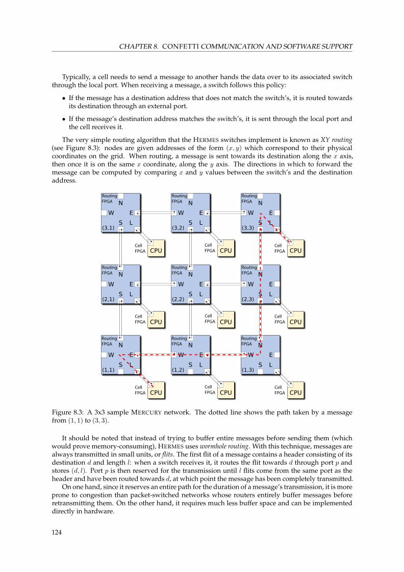
CHAPTER 8. CONFETTI COMMUNICATION AND SOFTWARE SUPPORT

Typically, a cell needs to send a message to another hands the data over to its associated switchthrough the local port. When receiving a message, a switch follows this policy:

• If the message has a destination address that does not match the switch’s, it is routed towardsits destination through an external port.

• If the message’s destination address matches the switch’s, it is sent through the local port andthe cell receives it.

The very simple routing algorithm that the HERMES switches implement is known as XY routing(see Figure 8.3): nodes are given addresses of the form (x, y) which correspond to their physicalcoordinates on the grid. When routing, a message is sent towards its destination along the x axis,then once it is on the same x coordinate, along the y axis. The directions in which to forward themessage can be computed by comparing x and y values between the switch’s and the destinationaddress.

RoutingFPGA

RoutingFPGA

RoutingFPGA

RoutingFPGA

RoutingFPGA

RoutingFPGA

RoutingFPGA

RoutingFPGA

RoutingFPGA

CellFPGA

CellFPGA

CellFPGA

CellFPGA

CellFPGA

CellFPGA

CellFPGA

CellFPGA

CellFPGA

Figure 8.3: A 3x3 sample MERCURY network. The dotted line shows the path taken by a messagefrom (1, 1) to (3, 3).

It should be noted that instead of trying to buffer entire messages before sending them (whichwould prove memory-consuming), HERMES uses wormhole routing. With this technique, messages arealways transmitted in small units, or flits. The first flit of a message contains a header consisting of itsdestination d and length l: when a switch receives it, it routes the flit towards d through port p andstores (d, l). Port p is then reserved for the transmission until l flits come from the same port as theheader and have been routed towards d, at which point the message has been completely transmitted.

On one hand, since it reserves an entire path for the duration of a message’s transmission, it is moreprone to congestion than packet-switched networks whose routers entirely buffer messages beforeretransmitting them. On the other hand, it requires much less buffer space and can be implementeddirectly in hardware.

124

8.4. TWO ADDITIONAL FUNCTIONAL UNITS FOR ULYSSE

8.3.4 MERCURY’s additions to HERMES

One of the main reason HERMES was chosen over different routing algorithms was the availabilityof its source code so that some changes and additions could be applied to accommodate our needs.These changes are of two kinds:

1. Serial protocolHERMES allows some flexibility in the version we started with, regarding the number of wiresused at low level to transport information. However, using a single line of data required tochange the routing core to take into account serialization and deserialization of data.

Moreover, HERMES initially used a FIFO to buffer a certain amount of flits during routing. How-ever, the usage of a serial protocol, requiring multiple clock cycles to transmit a single word,allowed us to remove this internal FIFO to save hardware.

2. Multiple clocksThe HERMES implementation relies heavily on the presence of single clock to synchronize itsinternal functioning. To accommodate our GALS platform, we had to insert adequate mech-anisms to ensure correct behavior in presence of multiple clocks. This translated into insert-ing handshaking mechanisms in the routing elements of HERMES. Luckily, this was relativelystraightforward as we could reuse some of the elements already present in HERMES and usethem with the MERCURY transceivers that also possess handshaking signals.

Thus, in total, every constituting component of HERMES was modified: if the routing algorithmitself was not modified in its essence, every other file was changed to take into account the transceiverpeculiarities as well as our clock requirements.

Routing performance analysis

Besides bandwidth measurements, no in-depth performance testing was undertaken with our im-plementation of HERMES, mostly because, qualitatively, the same performance figures obtained in[Moraes 04] are expected and also because the network performance has never been a limit to any ofour applications, the processor being the real bottleneck of the system.

However, should a more detailed outline be required, methods used in [Coppola 04] or [Pande 05]could be applied.

8.4 Two additional functional units for ULYSSE

To take into account the functionalities of the CONFETTI platform and leverage its advantages in theULYSSE processor, two functional units have been created: the first is a high-speed communication unitthat interfaces the HERMES network through a MERCURY transceiver and the second is a unit to giveULYSSE access to the LED screen and to the touch sensitive area to enable user input and interactions.

8.4.1 The MERCURY FU

As mentioned earlier, every FPGA on the routing substrate is physically linked to its four cardinalneighbors and to the cell board above it (Figure 8.4) using MERCURY interfaces. Thanks to our revisedHERMES implementation, every cell FPGA has now a connection to every other cell in the platformvia a routing algorithm. The role of the FU described here is to interface the ULYSSE processor to thatnetwork.

For this purpose, a MERCURY transceiver is also used to communicate from ULYSSE to the routingFPGA (see Figure 8.4). Embedded inside a complete functional unit, the transceiver gives ULYSSE adirect access to the underlying routing algorithm for sending and receiving data. As this algorithmis clearly separated from the computation happening in the processor itself, testing and developmentof the module was relatively simple. Additionally, this clear separation also implies that different

125

CHAPTER 8. CONFETTI COMMUNICATION AND SOFTWARE SUPPORT

Flash

High-speeddi�erential lines

Cell FPGA

Routing FPGA

Ulysseprocessor

Hermesswitch

Mercury interfaces

rdydtaclk

Figure 8.4: Detail of one routing FPGA and the link with its cell module.

Decodeheader

UpdateRAM 2

Wait fordata

Getheader

Get size

Idle

NOT empty_n

count=packet_size

NOT empty_n

empty_n

RAMrdy=1 & empty_nempty_n & new_data & (accept_dma |memory_valid_n)

rst_n

UpdateRAM 1

Figure 8.5: State machine of the receiver in ULYSSE MERCURY FU.

routing algorithms – be they based on HERMES or not – can be tested without changing this FU aslong as the low-level interface relies on MERCURY.

Data sending from ULYSSE consists of moving the data to be sent to the register embedded inthe FU. Reception is slightly more complex for performance reasons. In fact, we implemented adirect memory access (DMA) from the receiver to main memory so that incoming packets can becopied very fast from the interface to the memory. Without DMA, every word received would haverequired an explicit move operation from the FIFO to the memory, an operation that requires multipledisplacements to setup and execute, which would have rendered reception unnecessarily slow. Apacket reception is handled as follows (Figure 8.5): when new data arrives, if the unit is ready toaccept new packets, the header of the data is first decoded to extract the number of flits composingthe whole data stream; then, every time a new data word has been received and copied to memory(note that two cycles are required to perform this because memory access are 16-bit wide, see section3.7.2, page 40), a counter is incremented to determine when the reception is complete. During thewhole time the unit is waiting for new data to arrive, the processor is put in stalled state and the FUhas direct access to the memory. Of course, this presents the disadvantage that incomplete packetsblock the processor, which could be a problem. This situation can be prevented by adding a timeout

126

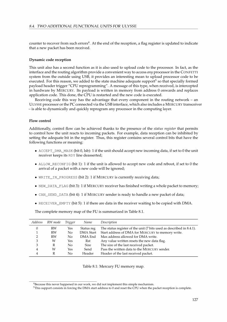
8.4. TWO ADDITIONAL FUNCTIONAL UNITS FOR ULYSSE

counter to recover from such errors4. At the end of the reception, a flag register is updated to indicatethat a new packet has been received.

Dynamic code reception

This unit also has a second function as it is also used to upload code to the processor. In fact, as theinterface and the routing algorithm provide a convenient way to access any processor in the CONFETTIsystem from the outside using USB, it provides an interesting mean to upload processor code to beexecuted. For this reason, we added to the state machine adequate support5 so that specially formedpayload header trigger “CPU reprogramming”. A message of this type, when received, is interceptedin hardware by MERCURY. Its payload is written in memory from address 0 onwards and replacesapplication code. This done, the CPU is restarted and the new code is executed.

Receiving code this way has the advantage that every component in the routing network – anULYSSE processor or the PC connected via the USB interface, which also includes a MERCURY transceiver– is able to dynamically and quickly reprogram any processor in the computing layer.

Flow control

Additionally, control flow can be achieved thanks to the presence of the status register that permitsto control how the unit reacts to incoming packets. For example, data reception can be inhibited bysetting the adequate bit in the register. Thus, this register contains several control bits that have thefollowing functions or meaning:

• ACCEPT_DMA_MASK (bit 0, lsb): 1 if the unit should accept new incoming data, if set to 0 the unitreceiver keeps its RDY line deasserted;

• ALLOW_RECONFIG (bit 1): 1 if the unit is allowed to accept new code and reboot, if set to 0 thearrival of a packet with a new code will be ignored;

• WRITE_IN_PROGRESS (bit 2): 1 if MERCURY is currently receiving data;

• NEW_DATA_FLAG (bit 3): 1 if MERCURY receiver has finished writing a whole packet to memory;

• CAN_SEND_DATA (bit 4): 1 if MERCURY sender is ready to handle a new packet of data;

• RECEIVER_EMPTY (bit 5): 1 if there are data in the receiver waiting to be copied with DMA.

The complete memory map of the FU is summarized in Table 8.1.

Address RW mode Trigger Name Description

0 RW Yes Status reg The status register of the unit (7 bits used as described in 8.4.1).1 RW No DMA Start Start address of DMA for MERCURY to memory write.2 RW No DMA End Max address allowed for DMA write.3 W Yes Rst Any value written resets the new data flag.3 R No Size The size of the last received packet.4 W Yes Send Pass the written data to the MERCURY sender.4 R No Header Header of the last received packet.

Table 8.1: Mercury FU memory map.

4Because this never happened in our work, we did not implement this simple mechanism.5This support consists in forcing the DMA start address to 0 and reset the CPU when the packet reception is complete.

127

CHAPTER 8. CONFETTI COMMUNICATION AND SOFTWARE SUPPORT

8.4.2 Display and interface FU

As the routing board also connects to the LED display, ULYSSE CPUs also have access to the screenportion that lies above them through a dedicated functional unit which uses a slower serial protocolthan MERCURY to communicate with the routing FPGA. Through this FU, each of the controllable 8x8pixels can be accessed with its address and its color changed, using 8 bit values for each of the threebasic color components (red-green-blue).

Additionally, through this FU the CPU can retrieve its X–Y coordinates in the global CONFETTIgrid and sense the value of the touch-sensitive area glued on it. Other registers are also accessible,notably used to access the content of the Flash memory containing the FPGA bitstreams for the cellboards6. Thus, these bitstreams can be accessed and modified directly from ULYSSE, for example tobe updated with new ULYSSE configuration or to implement a different processor than ULYSSE.

Table 8.2 reproduces the interface of this FU as seen by the processor. More details on its usagecan be found in the annexed listing B.1, page 231.

Address RW mode Trigger Name Description

0 R No X X-coordinate of this CPU in the CONFETTI grid.1 R No Y Y-coordinate of this CPU in the CONFETTI grid.0 W No Addr Address of the pixel to modify.1 W Yes Color Sets the color of the pixel.2 R No Touch # of seconds the touch sensor has been pressed continuously.3 R No Graphic Last pixel value written to the graphic memory.

[4. . . 7] RW No GR[0. . . 3] General purpose register [0. . . 3].

Table 8.2: Display FU memory map.

8.5 A software API for routing

Preliminary remark The forthcoming explanation on the software API is partly based, with his authoriza-tion, on Julien Ruffin’s work [Ruffin 08] who did his master thesis on the subject under my supervision.

Following the layered approach traditionally used in communication protocols, we implementedon top of the MERCURY physical layer a software transport layer that manages messages (Figure 8.6).The role of this component is to handle packet transmission and reception, providing more complexcommunication schemes than simple point-to-point communication. It consists of two essential parts:the first acts as a driver for MERCURY proper and provides simple send/receive functionality. Usingit, the second part implements useful operations such as broadcasting or guaranteed-delivery packets. Italso allows waiting for, then receiving, a packet fulfilling a set of given criteria.

8.5.1 Related work

As far as messaging layers are concerned, protocol stacks such as the one proposed by the Nostrumbackbone [Millberg 04] offer functionalities that largely exceed our needs in this project. In compar-ison, the communication system shown in the HS-Scale project [Saint-Jean 07] provides interestingfeatures that more closely resemble our needs, even though we designed simpler primitives than thedata sockets it offers. In fact, HS-Scale makes heavy use of interrupts and their absence in the ULYSSEprocessor required this simplification. Notably, polling has to be used for I/O operations and staticmultitasking is obtained with simple cyclic executives, meaning that the processor always executes

6Low-level access to the Flash modules is handled by the routing FPGA and is not detailed here. We refer the interestedreader to [Vannel 07].

128

8.5. A SOFTWARE API FOR ROUTING

Application

Transport

Network

Data link

Physical

7

4

3

2

1

Mercurylink

Hermesrouting

Mercurylink

Application

Transport

Network

Data link

Physical

7

4

3

2

1

Host /software

Media /hardware

mercury_send()

confiture_send()

mercury_send()

confiture_recv() Host /software

Media /hardware

Figure 8.6: Communication organization, based on OSI layers.

a single computation task. As we will see, notably in the next chapter, this peculiarity will not bewithout consequences in terms of efficiency.

8.5.2 The CONFITURE communication infrastructure

To simplify the use of messaging, we created a base library that is used as a layer between the MER-CURY low-level interface and user applications. Named CONFITURE, it implements a simple messag-ing system on top of the hardware and not only provides functionalities that derive from the hardwareimplementation but also adds its own special features.

Destination Length Sender Type Seq#88161616

Mercury Header Protocol extension

Figure 8.7: Message packet header format.

In practice, this layer extends MERCURY data packets – composed of a single word with destina-tion and length of the packet – into its own format to include sender, message type and sequencenumber information (Figure 8.7). This header consists of the following fields:

• destination The destination address, formatted as (x� 8) ‖ y.

• length The length of the payload of the message, including the CONFITURE header extension.

• sender The address of the message sender, in the same format as the destination.

• type Message types that can have the following values, based on the behavior required:

– Asynchronous, used for one-way messages. No reply is expected and waited by the library.

– Synchronous, used for messages that need to be confirmed when received. When sent, thelibrary function waits for an acknowledgment message from the recipient before consider-ing the send successful.

129

CHAPTER 8. CONFETTI COMMUNICATION AND SOFTWARE SUPPORT

– Broadcast, used for messages that are propagated to the entire grid. These messages exist intwo flavors, depending on their need to be acknowledged, i.e. a “synchronous” broadcastis considered correctly sent when all recipients acknowledge it.

– CPU reprogram, a special message that when received is intercepted in hardware by theULYSSE MERCURY FU. The payload of the message is then written to memory from address0 onwards and replaces application code. This done, the CPU is restarted. Because of this,CONFITURE provides functions to generate such messages but not to receive them.

• sequence number A user-managed field that can be used for example to store sequence informa-tion to reorder packets. It can also be used to define different messages subtypes.

Functions

CONFITURE offers base send() and receive() functions in two different variants, blocking or non-blocking.

Another pair of functions are provided for cell reprogramming. One replicates the node’s programto a given node address and the other, aptly named confiture_spread(), replicates the node’s pro-gram over the entire grid. This latest feature provides a very efficient way to distribute a source codeto the whole grid from the computer by reusing the same code and replicating it thanks to broad-cast functions, which undeniably reduces reprogramming time because the whole routing substrateis used in parallel. The replication mechanism used will be described in detail later in section 10.4.2.

The last function provided by CONFITURE is wait(), which blocks until a message whose headerfields match at least one (sender, type, seq#) tuple in a given list is received.

Even though we will limit our description of this library to this overview, the interested readerwill find in the annex, section B.2, the complete API of the library.

It is worth noting that, feature-wise, the additions of CONFITURE are separated from the way themessages are handled at low-level. Consequently, the code is also separated into two sub-layers: onethat contains the logic behind the additional features of CONFITURE7 while the second acts a driverfor MERCURY8. The advantage of this dual-layered approach is that CONFITURE could thus be portedto other networks than MERCURY by adapting the driver interface only.

Message queues

As mentioned earlier, an interesting constraint of the ULYSSE processor is its complete lack of inter-ruption support. This, as well as the inability to reliably do context switching, prevents any easy useof multitasking. The main consequence of this is that running multiple applications or a micro-kernelbased on timer interrupts is a non-trivial task on ULYSSE.

A common design used in messaging layers puts two message queues between the applicationand the messaging core proper. One of these queues is used for incoming messages and the otherfor outgoing messages; the application then reads in the first and writes in the second at will, themessaging system regularly filling the incoming queue and emptying the outgoing one, as long asthere are messages present.

This works well in multitasking systems where the messaging layer can handle buffers transpar-ently when needed, or in simpler systems using timer interrupts to periodically do the same. Sinceour system is neither multitasking nor able to use interrupts, any queue handling has to be manuallycalled by the application. This imposes a restriction upon applications using the messaging layer:they must consist of a loop alternating their own computation and passing control to the layer.

Such a restriction is a serious drawback. Considering also the potentially large memory require-ments of two queues, we decided to base CONFITURE on a radically different, simpler model. Gettingrid of queues nearly completely, CONFITURE executes operations directly when called without mes-sage buffering, blocking until their completion.

7In file confiture.h, annex p. 242.8In file mercury.h, annex p. 237.

130

8.5. A SOFTWARE API FOR ROUTING

All necessary handling – replying to “synchronous” messages, propagating broadcast messagesand waiting for acknowledgments – is done as needed directly at either message send or reception,blocking until successful completion or error. When a broadcast is sent for the first time or a “syn-chronous” message is sent, the send() function waits for a corresponding reply. Whenever CON-FITURE finds itself receiving a message from MERCURY that requires an acknowledgment in eitherthe receive() and wait() functions, the needed replies are sent before the message is properlydelivered.

As the layer implements wait() functions that block until the right message has been received, itis possible to receive messages while in that waiting state. Those messages are buffered in a small mes-sage queue dedicated to that purpose. The receive() function of CONFITURE first reads messagesoff this queue before querying MERCURY.

The broadcast algorithm

A naive way to implement broadcast would be to sequentially send the message to the whole nodegrid using a simple loop. Let N be the number of nodes in the grid: the same message then needsto be sent (N − 1) times by the initiating node. With a growing N , this becomes not only hard toaccomplish but extremely slow. The time needed to complete such a broadcast grows in O (N).

The solution we propose – and implemented – is more distributed. It uses two message types thatwe call Level-1 broadcast and Level-2 broadcast. To initiate a broadcast, a node sends the message to itsimmediate neighbors. On one axis of the grid, the node sends L1 broadcasts. On the axis orthogonalto it, L2 broadcasts are sent.

L2 broadcasts are propagated along the same axis by any node that receives it, as long as it stays inthe limits of the grid. L1 broadcasts are propagated in the same way, with the addition that they alsosend L2 messages along the orthogonal axis in the likeness of the initiating node. Figure 8.8 illustratesthe algorithm.

· · ·

Figure 8.8: CONFITURE broadcast example. Thick and thin arrows represent (resp.) L1 and L2 broad-cast messages.

This takes advantage of the mesh topology of CONFETTI’s architecture. The average time neededfor messages sent using this method to propagate themselves is by design directly related to theManhattan distance between the origin of the broadcast and the farthest nodes on the grid, whichgrows in O

(√N)

. We found square-root scalability sufficient for the desired applications and didnot consider more complex solutions, although some, such as [Al-Dubai 02], exist.

Another possible solution we set aside is the propagation of broadcast messages along a growingsquare centered on the initial sender. While faster from a propagation time standpoint, it requiresnodes at the corner of the square to propagate the message diagonally. This implies routing throughanother node in a direction to which a message was already sent, thus sending messages in the samedirection twice, which is not desirable.

Note that our broadcast has a guaranteed-delivery (“synchronous”) variant. With it, nodes thatpropagate the broadcast expect and wait for acknowledgment messages, sent back in the reverse pathof the broadcast messages. As such, when the initiating node receives all acknowledgments, it is sureall messages have been successfully received by the entire grid. The “asynchronous” variant does notsend acknowledgments and does not wait.

131

CHAPTER 8. CONFETTI COMMUNICATION AND SOFTWARE SUPPORT

8.6 A sample application: simulating synchronicity with CAFCA

In this section, we validate our hardware–software design approach by showing how a traditionalcellular automaton can be modeled within our framework. Cellular Automata (CA) date back tothe beginnings of Computer Science [Von Neumann 66]. By construction, they are a form of parallelcomputing. The following formal description is quoted from the introduction of [Mitchell 98]:

“A CA consists of two components. The first component is a cellular space: a lattice of Nidentical finite state machines (cells), each with an identical pattern of local connections toother cells for input and output, along with boundary conditions if the lattice is finite. LetΣ denote the set of states in a cell’s finite state machine, and k = |Σ| denote the number ofstates per cell. Each cell is denoted by an index i and its state at time t is denoted sti (wheresti ∈ Σ). The state sti of cell i together with the states of the cells to which cell i is connectedis called the neighborhood ηti of cell i.

The second component is a transition rule (or “CA rule”) φ(ηti) that gives the update states(t+1)i for each cell i as a function of ηti .

Typically in a CA a global clock provides an update signal for all cells: at each time stepall cells update their states synchronously according to φ(ηti).“

In other words, a CA is a set of identical cells aware of their state and that of their neighbors. Ateach time step, they use these data to update their state according to a transition rule. The variantwe are going to consider uses a two-dimensional lattice of square cells and updates their states in asynchronous, deterministic manner.

The task is not trivial because of the lack of global synchronization clocks in the CONFETTI system.Typically, this absence would imply a considerable effort on the programmer’s part to design andimplement alternative synchronization mechanisms, again requiring a strong knowledge of VHDLand of the detailed operation of the hardware.

Main Loop

Initialization

state update

round start

next state

display

messaging

internalinitialization

state display

state computation

init

wait

send

CAFCAMessaging layer User code for CA

Figure 8.9: Structure of an application using CAFCA. Arrows represent function calls.

To overcome this limitation, we developed CAFCA (Cellular Automata Framework for Cellular Ar-chitectures), a software library that runs on the ULYSSE processor and that essentially permits, thanksto the messaging layer, to virtualize the fact that we are running a globally asynchronous system.

This tool represents a good example of the kind of software interfaces that can allow virtually anyresearcher to exploit the power of bio-inspired hardware implementations. In fact, when using thislibrary it becomes then possible to develop parallel applications based on the cellular automata modelby writing only a few C functions without any particular knowledge of the hardware. Because thedevelopment of the library had to be done only once, it greatly enhances the usability of the system.

132

8.7. CONCLUSION AND FUTURE WORK

To achieve a synchronized behavior, a step in the cellular automaton model implemented byCAFCA consists of four phases:

• Synchronization: all nodes wait for a broadcast message indicating the beginning of a computa-tion round. If the node is the “coordinator” node (see below), it sends a synchronous broadcastto synchronize all the other cells.

• Inter-neighbor state exchange: information with the neighbors nodes is exchanged using simpleasynchronous messages.

• Next state update: the value of the next state is computed from the node’s own state and that ofthe neighbors.

• Display: the newly-computed state is sent to the LED display.

CAFCA builds upon the messaging layer and leverages the grid topology of the underlying hard-ware to provide cell synchronization and state exchange between neighbors that belong to differentclock domains. Technically speaking, this is implemented with one of the cells, the “coordinator”,playing the role of a supervisor to ensure, using broadcast messages, that every cell is at the samestep.

Regarding the implementation, the coordinator’s address and the initialization function pointerare the only CAFCA-specific arguments, respectively telling which node should be the coordinatorand providing a pointer to the application’s startup code. As a side note, it is possible to switchbetween Von Neumann and Moore neighborhoods with a compilation parameter. Wrapping is alsoprovided by CAFCA. Thus, the cell space can be toroidal if needed: if a cell’s neighbor happen to beoutside the physical cell grid, the cell at the opposite end of the grid is accessed, “wrapping around”the coordinate axis. This feature is greatly facilitated by message routing.

An application that uses the framework library needs to provide only the functions for the com-putation and display phases, as well as emplacements to store local/neighbor states and their size, asshown on Figure 8.9. By fully handling synchronization and messaging issues, CAFCA enables fastdevelopment strictly centered on the two defining characteristics of a cellular automaton – the statevariables and the state update function.

As an example, a simple implementation of Conway’s Game of Life [Gardner 85] in our frameworktakes less than 100 lines of C code (corresponding to the user code in Figure 8.9). A complete versionwith 64 cells simulated per processor requires a total of about 200 lines of C code (the complete code isreproduced in the annex on page 245). A simplified version, showing a glider in 64 cells per processor,is shown in Listing 8.1.

Other examples we developed, such as a basic version of heat distribution in an homogeneousmetal plate or the simulation of shallow water equations, can be coded in less than one thousandlines. Listing B.5 (p. 248) exemplifies the flexibility of the library by showing how different borderconditions can be easily implemented. Figure 8.10 displays some pictures that were taken during theexecution of various cellular automata9.

8.7 Conclusion and future work

In addition to hardware routing in CONFETTI, which completes the description of our platform, weshowed in this chapter a first type of application that can be realized with it.

As an example of the type of tools that could be invaluable for research in bio-inspired hard-ware, we showed how the framework we have developed can be used to provide an easy and rapidimplementation of a traditional task for cellular hardware systems in the form of cellular automata.By developing several hardware and software components, we were able to drastically reduce thenon-recurrent engineering time generally implied by the usage of intimately linked hardware and

9Videos showing some examples of the library usage on CONFETTI can be found at http://birg.epfl.ch/page69673.html

133

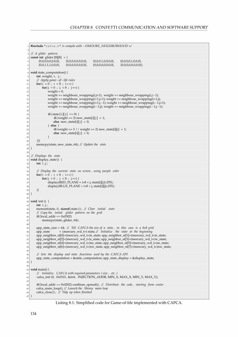
CHAPTER 8. CONFETTI COMMUNICATION AND SOFTWARE SUPPORT

1 #include "cafca.h" /∗ compile with −DMOORE_NEIGHBORHOOD ∗/2

3 // A glider pattern4 const int glider [8][8] = {5 {0,0,0,0,0,0,0,0}, {0,0,0,0,0,0,0,0}, {0,0,0,1,0,0,0,0}, {0,0,0,0,1,0,0,0},6 {0,0,1,1,1,0,0,0}, {0,0,0,0,0,0,0,0}, {0,0,0,0,0,0,0,0}, {0,0,0,0,0,0,0,0}};7

8 void state_computation() {9 int weight, i , j ;

10 // Apply game−of−life rules11 for( i = 0 ; i < 8 ; i++) {12 for( j = 0 ; j < 8 ; j++) {13 weight = 0;14 weight += neighbour_wrapping(i,j+1); weight += neighbour_wrapping(i,j−1);15 weight += neighbour_wrapping(i+1,j+1); weight += neighbour_wrapping(i+1,j);16 weight += neighbour_wrapping(i+1,j−1); weight += neighbour_wrapping(i−1,j+1);17 weight += neighbour_wrapping(i−1,j); weight += neighbour_wrapping(i−1,j−1);18

19 if ( state [ i ][ j ] == 0) {20 if (weight == 3) new_state[i][ j ] = 1;21 else new_state[i][ j ] = 0;22 } else {23 if (weight == 3 || weight == 2) new_state[i][j ] = 1;24 else new_state[i][ j ] = 0;25 }26 }}}27 memcpy(state, new_state, 64); // Update the state28 }29

30 // Displays the state31 void display_state() {32 int i , j ;33

34 // Display the current state on screen , using purple color35 for( i = 0 ; i < 8 ; i++) {36 for( j = 0 ; j < 8 ; j++) {37 display(RED_PLANE + i∗8 + j, state[i][j]∗255) ;38 display(BLUE_PLANE + i∗8 + j, state[i][j]∗255) ;39 }}40 }41

42 void init () {43 int i , j ;44 memset(state, 0, sizeof( state ) ) ; // Clear initial state45 // Copy the initial glider pattern on the grid46 if (local_addr == 0x0302)47 memcpy(state, glider, 64) ;48

49 app_state_size = 64; // Tell CAFCA the size of a state , in this case is a 8x8 grid50 app_state = (mercury_wd_t∗) state; // Initialize the state at the beginning51 app_neighbor_st[0]=(mercury_wd_t∗)n_state; app_neighbor_st[1]=(mercury_wd_t∗)e_state;52 app_neighbor_st[2]=(mercury_wd_t∗)s_state; app_neighbor_st[3]=(mercury_wd_t∗)w_state;53 app_neighbor_st[4]=(mercury_wd_t∗)ne_state; app_neighbor_st[5]=(mercury_wd_t∗)se_state;54 app_neighbor_st[6]=(mercury_wd_t∗)sw_state; app_neighbor_st[7]=(mercury_wd_t∗)nw_state;55

56 // Sets the display and state functions used by the CAFCA API57 app_state_computation = &state_computation; app_state_display = &display_state;58 }59

60 void main() {61 // Initialize CAFCA with required parameters ( size , etc .)62 cafca_init (0, 0x0101, &init, INJECTION_ADDR, MIN_X, MAX_X, MIN_Y, MAX_Y);63

64 if (local_addr == 0x0202) confiture_spread(); // Distribute the code , starting from center65 cafca_main_loop(); // Launch the library main loop66 cafca_close () ; // Tidy up when finished67 }

Listing 8.1: Simplified code for Game-of-life implemented with CAFCA.

134

8.7. CONCLUSION AND FUTURE WORK

(a) Game of life (b) Fire

(c) Heat dissipation (d) Shallow water equation

Figure 8.10: CAFCA examples.

software. This was achieved by delegating all the complexity to a framework which presents to theprogrammer a simplified, yet powerful, view of the system. Thus, with a tool such as CAFCA, everyprogrammer that knows C could exploit the computational power of hundreds of FPGAs with just afew lines of standard code.

A further development of the platform itself would be to implement virtual channels [Mello 05,Mello 06] to provide QoS guarantees on communication. Another interesting topic would consistof replacing ULYSSE with a more standard processor to analyze the impact of the TTA paradigm onperformance at system level.

Regarding further developments of the software presented in this chapter, the implementation ofother software libraries could, for example, take advantage of the reconfigurability of the system toimplement growth or replication but also to realize computationally-intensive functions such as videodecoding by implementing ad-hoc FUs.

In the next chapter, we will examine how different software tools can be designed to help easilydevelop applications for complex hardware platforms such as the one we just presented.

135

Bibliography

[Al-Dubai 02] A. Y. Al-Dubai, M. Ould-Khaoua & L. M. Mackenzie. Towards a scalable broad-cast in wormhole-switched mesh networks. In Proceedings of the 2002 ACMsymposium on Applied computing (SAC’02), pages 840–844, New York, USA,2002. ACM.

[Amde 05] M. Amde, T. Felicijan, A. Efthymiou, D. Edwards & L. Lavagno. Asyn-chronous On-Chip Networks. IEE Proceedings Computers and Digital Tech-niques, vol. 152, no. 2, March 2005.

[Andriahantenaina 03] A. Andriahantenaina & A. Greiner. Micro-network for SoC: implementation of a32-port SPIN network. In Proceedings of the conference on Design, automationand test in Europe (DATE’03), pages 1128–1129, 2003.

[Bartic 05] T.A. Bartic, J.-Y. Mignolet, V. Nollet, T. Marescaux, D. Verkest, S. Vernalde& R. Lauwereins. Topology adaptive network-on-chip design and implementation.IEE Proceedings – Computers and Digital Techniques, vol. 152, no. 4, pages467–472, 2005.

[Benini 01] Luca Benini & Giovanni de Micheli. Power networks on chips: energy-efficientand reliable interconnect design for SoCs. In Proceedings of the 14th InternationalSymposium on Systems Synthesis (ISSS’01), pages 33–38, October 2001.

[Benini 02] Luca Benini & Giovanni de Micheli. Networks on Chips: A New SoC Paradigm.Computer, vol. 35, no. 1, pages 70–78, 2002.

[Coppola 04] Marcello Coppola, Stephane Curaba, Miltos D. Grammatikakis, Riccardo Lo-catelli, Giuseppe Maruccia & Francesco Papariello. OCCN: a NoC modelingframework for design exploration. Journal of Systems Architecture, vol. 50, no. 2-3, pages 129–163, 2004.

[Dally 01] William J. Dally & Brian Towles. Route packets, not wires: on-chip inteconnectionnetworks. In DAC ’01: Proc. 38th Conf. on Design automation, pages 684–689,New York, USA, 2001. ACM Press.

[Day 83] John D. Day & Hubert Zimmermann. The OSI reference model. Proceedings ofthe IEEE, vol. 71, no. 12, pages 1334–1340, 1983.

[de Micheli 06] Giovanni de Micheli & Luca Benini. Networks on Chips: Technology and Tools(Systems on Silicon). Morgan Kaufmann, first edition, 2006.

[Duato 02] Jose Duato, Sudhakar Yalamanchili & Lionel Ni. Interconnection Networks: AnEngineering Approach. Elsevier Science, revised edition, 2002.

[Dumitras 03] Tudor Dumitras, Sam Kerner & Radu Marculescu. Towards on-chip fault-tolerant communication. In ASPDAC: Proceedings of the 2003 conference onAsia South Pacific design automation, pages 225–232, New York, USA, 2003.ACM.

137

BIBLIOGRAPHY

[Gardner 85] Martin Gardner. Wheels, Life, and Other Mathematical Amusements. W.H. Free-man & Company, 1985.

[Guerrier 00] P. Guerrier & A. Greiner. A generic architecture for on-chip packet-switched inter-connections. In Proceedings of the conference on Design, automation and testin Europe (DATE’00), pages 250–256, 2000.

[Karim 02] F. Karim, A. Nguyen & S. Dey. An interconnect architecture for networking sys-tems on chips. IEEE Micro, vol. 22, no. 5, pages 36–45, 2002.

[Kumar 02] S. Kumar, A. Jantsch, J.P. Soininen, M. Forsell, M. Millberg, J. Oberg, K. Tien-syrja & A. Hemani. A network on chip architecture and design methodology. InIEEE Computer Society Annual Symposium on VLSI (ISVLSI’02), pages 105–112, April 2002.

[Liang 00] Jian Liang, Sriram Swaminathan & Russell Tessier. aSOC: A Scalable, Single-Chip Communications Architecture. In Proceedings of the International Con-ference on Parallel Architectures and Compilation Techniques, vol. 0, pages37–46, Los Alamitos, CA, USA, 2000. IEEE Computer Society.

[Marescaux 02] Théodore Marescaux, Andrei Bartic, Diederik Verkest, Serge Vernalde &Rudy Lauwereins. Interconnection Networks Enable Fine-Grain Dynamic Multi-tasking on FPGAs. In Proceedings of 12th International Conference on Field-Programmable Logic and Applications (FPL ’02) - The Reconfigurable Com-puting Is Going Mainstream, pages 795–805, London, UK, 2002. Springer-Verlag.

[Marescaux 03] Théodore Marescaux, Jean-Yves Mignolet, Andrei Bartic, W. Moffat, DiederikVerkest, Serge Vernalde & Rudy Lauwereins. Networks on Chip as HardwareComponents of an OS for Reconfigurable Systems. In Proceedings of 13th Inter-national Conference on Field Programmable Logic and Applications (FPL’03),pages 595–605, 2003.

[Mello 05] Aline Mello, Leonel Tedesco, Ney Calazans & Fernando Moraes. Virtual Chan-nels in Networks on Chip: Implementation and Evaluation on Hermes NoC. In Pro-ceedings of the 18th Symposium on Integrated Circuits and Systems Design(SBCCI’05), pages 178–183. ACM, 2005.

[Mello 06] Aline Mello, Leonel Tedesco, Ney Calazans & Fernando Moraes. Evaluationof current QoS Mechanisms in Networks on Chip. In Proceedings of the Interna-tional Symposium on System-on-Chip, pages 1–4, November 2006.

[Millberg 04] Mikael Millberg, Erland Nilsson, Rikard Thid, Shashi Kumar & Axel Jantsch.The Nostrum Backbone - a Communication Protocol Stack for Networks on Chip. InProceedings of the 17th International Conference on VLSI Design (VLSID’04),page 693, Washington, USA, 2004. IEEE Computer Society.

[Mitchell 98] Melanie Mitchell. Computation in Cellular Automata: A Selected Review. InNonstandard Computation, pages 95–140. VCH Verlagsgesellschaft, 1998.

[Moraes 04] Fernando Moraes, Ney Calazans, Aline Mello, Leandro Möller & Luciano Ost.HERMES: an infrastructure for low area overhead packet-switching networks on chip.Integrated VLSI Journal, vol. 38, no. 1, pages 69–93, 2004.

[Murali 06] Srinivasan Murali, David Atienza, Luca Benini & Giovanni de Micheli. AMulti-Path Routing Strategy with Guaranteed In-order Packet Delivery and FaultTolerance for Networks on Chips. In Proceedings of the Design Automation Con-ference (DAC’06), pages 845–848, 2006.

138

BIBLIOGRAPHY

[Murali 07] Srinivasan Murali, David Atienza, Luca Benini & Giovanni de Micheli. Amethod for routing packets across multiple paths in NoCs with in-order delivery andfault-tolerance guarantees. VLSI Design, vol. 2007, page 11, 2007.

[Ngouanga 06] Alex Ngouanga, Gilles Sassatelli, Lionel Torres, Thierry Gil, André Soares& Altamiro Susin. A contextual resources use: a proof of concept through theAPACHES’ platform. In Proceedings of the IEEE Workshop on Design and Di-agnostics of Electronic Circuits and Systems (DDECS’06), pages 44–49, April2006.

[Ni 93] Lionel M. Ni & Philip K. McKinley. A Survey of Wormhole Routing Techniquesin Direct Networks. IEEE Computer, vol. 26, no. 2, pages 62–76, 1993.

[Pande 05] Partha Pratim Pande, Cristian Grecu, André Ivanov, Resve Saleh & Giovannide Micheli. Design, Synthesis, and Test of Network on Chips. IEEE Design & Testof Computers, vol. 22, no. 5, pages 404–413, 2005.

[Rijpkema 01] Edwin Rijpkema, Kees Goossens & Paul Wielage. A Router Architecture for Net-works on Silicon. In Proceedings of the 2nd Workshop on Embedded Systems(Progress’01), pages 181–188, 2001.

[Ruffin 08] Julien Ruffin. Self-organized Parallel Computation on the CONFETTI Cellular Ar-chitecture. Master’s thesis, École Polytechnique Fédérale de Lausanne, 2008.

[Saint-Jean 07] Nicolas Saint-Jean, Gilles Sassatelli, Pascal Benoit, Lionel Torres & MichelRobert. HS-Scale: a Hardware-Software Scalable MP-SOC Architecture for em-bedded Systems. In Proceedings of the IEEE Computer Society Annual Sympo-sium on VLSI (ISVLSI’07), pages 21–28, 2007.

[Teehan 07] Paul Teehan, Mark Greenstreet & Guy Lemieux. A Survey and Taxonomy ofGALS Design Styles. IEEE Design and Test, vol. 24, no. 5, pages 418–428, 2007.

[Vannel 07] Fabien Vannel. Bio-inspired cellular machines: towards a new electronic paper ar-chitecture. PhD thesis, École Polytechnique Fédérale de Lausanne, Lausanne,2007.

[Von Neumann 66] John Von Neumann. Theory of Self-Reproducing Automata. University of IllinoisPress, Champaign, IL, USA, 1966.

[Wiklund 03] Daniel Wiklund & Dake Liu. SoCBUS: Switched Network on Chip for Hard RealTime Embedded Systems. In Proceedings of the 17th International Symposiumon Parallel and Distributed Processing (IPDPS’03), page 78.1, Washington,USA, 2003. IEEE Computer Society.

[Ye 03] Terry Tao Ye, Luca Benini & Giovanni de Micheli. Packetized On-Chip Intercon-nect Communication Analysis for MPSoC. In Proceedings of the conference onDesign, automation and test in Europe (DATE’03), vol. 1, pages 344–349, LosAlamitos, CA, USA, March 2003. IEEE Computer Society.

139

Chapter 9

A software environment for cellularcomputing

“A worker may be the hammer’s master, but the hammer still prevails.A tool knows exactly how it is meant to be handled,

while the user of the tool can only have an approximate idea.”

MILAN KUNDERA, The Book of Laughter and Forgetting

THE APPLICATION of bio-inspired mechanisms such as evolution, growth or self-repair in hardwarerequires resources (fault-detection logic, self-replication mechanisms, . . . ) that are normally not

available in off-the-shelf circuits. For these reasons, a number of dedicated hardware devices weredeveloped, e.g. [Greensted 07,Tempesti 01,Thoma 04,Upegui 07], with the intent of exploring variousbio-inspired paradigms.

In general however, they represent experimental platforms that are very difficult to program andrequire an in-depth understanding of the underlying hardware. As a consequence, these platformsare accessible only to a limited class of programmers who are well-versed in hardware descriptionlanguages (such as VHDL) and who are willing to invest considerable time in learning how to designhardware for a specific, often ill-documented, device.

Notwithstanding these issues, hardware remains an interesting option in this research domain asit can greatly accelerate some operations and because it allows a direct interaction with the environ-ment. It is however undeniable that the difficulty of efficiently programming hardware platforms hasprevented their use for complex real-world applications. In turn, the fact that experiments have beenmostly limited to simple demonstrators has hindered the widespread acceptance of the bio-inspiredtechniques they were meant to illustrate.

While, by their very nature, bio-inspired systems rely on non-conventional mechanisms, in themajority of cases they bear some degree of similarity to networks of computational nodes, a structurethat is frequently used when dealing with parallel computing systems. In these latter, a softwareabstraction is often used to hide the complexity and details of the underlying hardware and simplifyprogramming. It is therefore legitimate to wonder if such an approach can be applied to bio-inspiredhardware systems as well, to allow researchers to rapidly prototype new ideas and, more importantly,to cope with the complexity of tens or hundreds of parallel computational elements.

In this chapter we describe a set of software tools, gathered in a graphical user interface (GUI),that attempt to help the user with intuitive hints during the critical phases of the design of distributedcellular architectures. More precisely, we will present a software framework that provides a model ofsystems such as CONFETTI to simplify their programming thanks to a strict separation of the hardwareand software. We will see that with this framework, deliberately open and modular so that it can beeasily extended with new modules, it becomes possible to quickly evaluate performance, algorithms,techniques and ideas for the community of researchers interested in bio-inspired hardware.

141

CHAPTER 9. A SOFTWARE ENVIRONMENT FOR CELLULAR COMPUTING

9.1 Introduction and motivations

Although the hardware in almost every desktop computer sold nowadays offers the possibility ofexecuting multiple threads in parallel, a majority of the software written for these machines remainsserial. This situation can be explained, at least partly, by the complexity of writing multithreadedapplications: when multiple threads run in concert, the sequential model of programming breaksdown. For example, the apparition of shared variables necessarily translates to concurrent accesses,which in turn requires to analyze program functions with a broader view than usual, the programmerhaving to think outside the scope of the function.

Of course, several programming languages propose techniques to reduce the complexity penaltyof introducing parallelism: for instance, functional languages such as Haskell1 [Hutton 07] do notinclude the notion of shared state nor that one of sequential execution, and other languages, such asAPL [Iverson 62], remove the limitation of doing a single thing at a time. However, all these languagesare not widespread and they lack the acceptance and backing of the C/C++ or Java languages. Thus,the solution generally used to help parallel programming with more “traditional” languages relies onlibraries, such as the Message Passing Interface (MPI) [Snir 96], that provide an abstraction layer betweenthe parallel system where the application is executed and its software counterpart.

One of the stated objectives of this thesis is to generalize the use of bio-inspired techniques, no-tably in the context of cellular computing. As we have already mentioned, this latter bears some sim-ilarities with parallel programming, although with notable differences in terms of resource availablewhen compared to desktop computing but also in terms of OS stability, desktop computers benefitingfrom software with years of development behind them. Thus, the direct translation of such a libraryis difficult or even impossible, notably due to the heavy resource constraints present in embeddedsystems.

In our opinion, the development of an approach similar to the one proposed by MPI could behelpful for cellular computing in embedded systems: in fact, the need of an intermediate layer tocreate distance between the low-level hardware and the software representation of that hardware iseven more acute in such systems because they often lack a proper operating system that plays thisrole.

In this chapter, we present such a software for our cellular approach, with the main objective ofproposing an unified environment for cellular computing so that any user can rapidly handle complexparallel computing platforms without having to master the nitty-gritty details of that hardware. Thesecondary objective of the interface-based program is to maintain a high level of flexibility so that newcomponents can be easily added to accommodate the needs of different users, different applicationsand rapidly prototype new ideas. In other words, our intention in this chapter is to propose toolsto help embedded developers tackle the problems that arise concurrently with the advent of parallelembedded systems. To achieve this goal we will proceed as follows: in the next section we will presentand justify the validity of the program model we use, which consists in specifying applications as agraph of tasks using a visual interface. We will then present a general overview of the applicationin section 9.4, which articulates around two distinct sets of tools. The first one, aimed at helping theuser create the core functions of the programs, will be detailed in section 9.5. The second set of toolsprovides support for developing and analyzing task graphs, notably thanks to two different graphsimulation environments.

9.2 Graphical programming languages

Visual or graphical programming languages let users create applications by manipulating visually theconstituting elements of a program where a traditional specification would require a textual approach.Thus, the majority of these languages use graphical objects connected together to represent the rela-tions between the various program entities. Often used to describe systems with concurrency issues,visual languages such as Petri nets [Peterson 81] have been notably used to model parallel systems,

1See http://www.haskell.org

142

9.3. A PROGRAMMING MODEL

tackling issues such as resource sharing. More recently, these languages have shown a revamped in-terest because they can be used to represent efficiently dataflow programming (see section 9.3.2), aparadigm which has been identified as a promising candidate for the automatic parallelization of pro-grams [Johnston 04]. In the context of this thesis, the advantage of using such a visual programminglanguage is three-fold:

1. simplify the development of parallel programs by providing a visual and intuitive way to expressapplications in terms of objects linked together;

2. provide a visual feedback of the performance and behavior of the application;

3. create a clear distinction between the software, which is expressed visually to illustrate abstrac-tions, and the hardware itself, which is absent from that visual description.

Naturally, the idea of using a GUI interface for studying and creating parallel programs is not, initself, new. For instance, in 1990, Lewis et al. [Lewis 90] proposed a tool for scheduling large-grainparallel program tasks under the assumption that “the best solutions are obtained in cooperation witha human designer” [Lewis 90, p. 1172]. This statement is based on the observation that, due to thevery different nature of existing problems that might have to be solved by parallel systems, relyingto some extent on human expertise during the design cycle is a good idea, an opinion that we share.As a result, the software GUI we propose contains several components that help the user make gooddecisions, for example with tools to graphically model parallel programs using task graphs or with atool to observe different performance estimates of the program.

Regarding the need for a distinct separation between hardware and software, recent works under-line the importance of the concept, notably for embedded systems. Thus, Engler et al. [Engler 95] orNesbit et al. [Nesbit 08] have shown the advantages of using the notion of virtual machines with whicha software layer can be used to implement policies whilst the hardware provides mechanisms to sup-port them. Even though we will not use the virtual machine paradigm in this work, the approachwe use bears some similarities with the concept in that it uses an interface between hardware andsoftware, an approach also proposed for example in the work of van der Wolf et al. [van der Wolf 04],who stress the importance of such a layer:

“[this interface] should help to close the gap between the application models used forspecification and the optimized implementation of the application on a multi-processorarchitecture [...] Such interface and mapping technology will help to structure MPSoCintegration, thereby enhancing both the productivity and the quality of MPSoC design.”[van der Wolf 04, p. 206]

9.3 A programming model

If visual programming languages allow to manipulate programs, a model for these programs is stillrequired. Luckily, the literature is rich with different solutions for this question. The one we use inthis work is one of the most commonly used, i.e. the directed acyclic graph (DAG) model. Even thoughother interesting alternatives can also be used, such as Kahn process networks [Kahn 74], DAGs aresimple enough to model our needs and are also more widespread, which implies that the considerablework done on this kind of applications could also be applied to suit our current or future needs.

9.3.1 Directed acyclic graphs programs

Definition A directed acyclic graph program is a directed graph without cycles in which vertices rep-resent tasks, characterized by an execution cost, whose connections to other vertices through edgesrepresent precedence relations, potentially characterized by a communication cost [Sarkar 89].

143

CHAPTER 9. A SOFTWARE ENVIRONMENT FOR CELLULAR COMPUTING

a

Kernel 1cost = 1

Kernel 2cost = 3

1

Kernel 4cost = 2

2

b

Kernel 3cost = 4

2

cd

1

output

(a) DAG

// Kernel_1void compute(input, output){output[0] = input[0] + 10;

}

// Kernel_2void compute(input, output){output[0] = input[0] * input[1];

}

// Kernel_3void compute(input, output){output[0] = pow(input[0], input(1));

}

// Kernel_4void compute(input, output){output[0] = input[0] + input[1] - input[2];

}

(b) Corresponding code

Figure 9.1: Sample of an application in DAG form with its corresponding pseudo-code.

Figure 9.1 shows how this graph representation can be used to model a simple parallel programthat computes the value of a+(a+10) · d−(bc). In the graphic representation, each node2 is representedas an ellipse and the execution time of the task is written inside it, whereas the communication cost iswritten on each edge. In this model, a task is triggered (i.e. starts working) when all its predecessorshave produced an output that is then used as an input for the successor node (also known as theasynchrony property, see [Gajski 82]). The second property of the model is called the functionalityproperty (see [Gajski 82]): as every operation is a function and no shared memory is used, side effectsare impossible, i.e. no state is modified in addition to returning a value.

DAGs have been used in the literature to examine notions such as scheduling, a NP-hard prob-lem [Garey 79] which consists in minimizing the total execution time (also called makespan or schedulelength) of parallel programs, by allocating tasks to processors so that the precedence order is main-tained [Ahmad 99]. However, if DAGs can be used to describe the relations between the tasks, theydo not stipulate how the application itself is programmed. As such, they can be considered as a con-ceptual modeling tool for parallel programs to which a programming model should be added to be usedin real situations and that will be examined in the next subsection.

9.3.2 Dataflow / stream programming

The dataflow programming paradigm is a form of parallel processing that simplifies the developmentof certain types of applications, at the expense of some limitations. This model makes use of kernelfunctions, represented with a DAG, that are applied to a set of data called the data stream. In this DAG,the vertices represent the kernel functions and the edges account for the precedence relations takenby the data stream.

The stream programming paradigm closely resembles the dataflow paradigm, with the notable dif-ference that the former tends to consider computation at a lower lever, closer to the machine. In theremainder of this work, these two concepts should be seen as synonyms, even though a differenceexists in terms of the implementation of the model.

Multiple languages were developed with these paradigms as a cornerstone, such as the StreamITlanguage at MIT [Thies 02, Gordon 06], the Brook language at Stanford [Buck 04] or Intel’s Ct [Ghu-loum 07] (which is a proprietary language). These languages were mainly developed for specificso-called stream processors, such as the Stanford Imagine [Kapasi 02] and Merrimac [Dally 03], the MITRAW [Taylor 02] or to a certain extent the Sony-Toshiba-IBM Cell [Pham 06]. However, the scope of

2In this thesis, the terms tasks and nodes have the same meaning and are used indifferently.

144

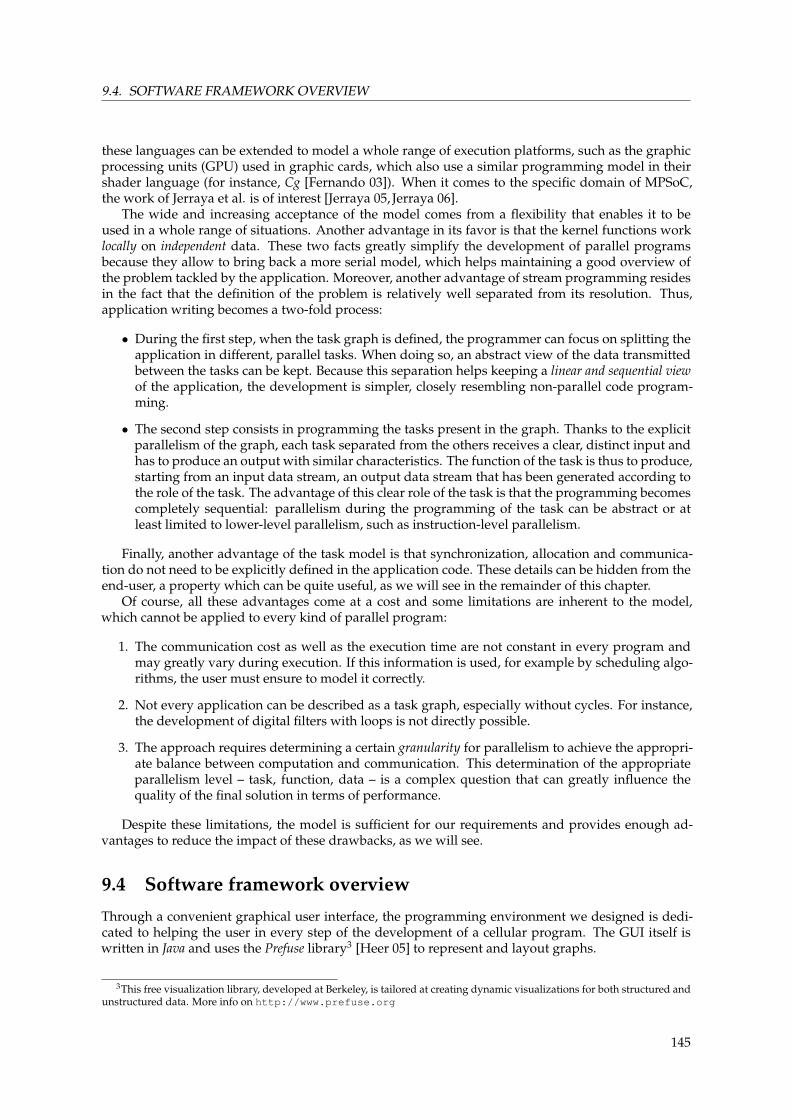
9.4. SOFTWARE FRAMEWORK OVERVIEW

these languages can be extended to model a whole range of execution platforms, such as the graphicprocessing units (GPU) used in graphic cards, which also use a similar programming model in theirshader language (for instance, Cg [Fernando 03]). When it comes to the specific domain of MPSoC,the work of Jerraya et al. is of interest [Jerraya 05, Jerraya 06].

The wide and increasing acceptance of the model comes from a flexibility that enables it to beused in a whole range of situations. Another advantage in its favor is that the kernel functions worklocally on independent data. These two facts greatly simplify the development of parallel programsbecause they allow to bring back a more serial model, which helps maintaining a good overview ofthe problem tackled by the application. Moreover, another advantage of stream programming residesin the fact that the definition of the problem is relatively well separated from its resolution. Thus,application writing becomes a two-fold process:

• During the first step, when the task graph is defined, the programmer can focus on splitting theapplication in different, parallel tasks. When doing so, an abstract view of the data transmittedbetween the tasks can be kept. Because this separation helps keeping a linear and sequential viewof the application, the development is simpler, closely resembling non-parallel code program-ming.

• The second step consists in programming the tasks present in the graph. Thanks to the explicitparallelism of the graph, each task separated from the others receives a clear, distinct input andhas to produce an output with similar characteristics. The function of the task is thus to produce,starting from an input data stream, an output data stream that has been generated according tothe role of the task. The advantage of this clear role of the task is that the programming becomescompletely sequential: parallelism during the programming of the task can be abstract or atleast limited to lower-level parallelism, such as instruction-level parallelism.

Finally, another advantage of the task model is that synchronization, allocation and communica-tion do not need to be explicitly defined in the application code. These details can be hidden from theend-user, a property which can be quite useful, as we will see in the remainder of this chapter.

Of course, all these advantages come at a cost and some limitations are inherent to the model,which cannot be applied to every kind of parallel program:

1. The communication cost as well as the execution time are not constant in every program andmay greatly vary during execution. If this information is used, for example by scheduling algo-rithms, the user must ensure to model it correctly.

2. Not every application can be described as a task graph, especially without cycles. For instance,the development of digital filters with loops is not directly possible.

3. The approach requires determining a certain granularity for parallelism to achieve the appropri-ate balance between computation and communication. This determination of the appropriateparallelism level – task, function, data – is a complex question that can greatly influence thequality of the final solution in terms of performance.

Despite these limitations, the model is sufficient for our requirements and provides enough ad-vantages to reduce the impact of these drawbacks, as we will see.

9.4 Software framework overview

Through a convenient graphical user interface, the programming environment we designed is dedi-cated to helping the user in every step of the development of a cellular program. The GUI itself iswritten in Java and uses the Prefuse library3 [Heer 05] to represent and layout graphs.

3This free visualization library, developed at Berkeley, is tailored at creating dynamic visualizations for both structured andunstructured data. More info on http://www.prefuse.org

145

CHAPTER 9. A SOFTWARE ENVIRONMENT FOR CELLULAR COMPUTING

User driven

Automated

Shape legend

Color legendSoftware execution

Hardware execution

Tasks programming

Application de�nition

Application splittingin tasks

C code programusing templates

Task graph

Compile task

Tasks placement Timingsimulation

Parallelsimulation

Graph compilation

Functional veri�cation

Code correction

Simulated traceanalysis

Trace analysis

Optimization

OptimizationOptimization

Application veri�cation

Code correction

Static execution Dynamic execution

Pro�ling

Pro�le analysis

Task simulation

Optimization

a

b

c

de

f

Figure 9.2: Development environment for cellular programming.

146

9.5. TASK PROGRAMMING TOOLS

A general overview of the functionalities of the applications is depicted in Figure 9.2, which showshow the different phases of the programming process interact4. Following that diagram, the outlineof a typical programming session in the GUI is as follows:

1. For each application, the user starts by manually analyzing and splitting the application intotasks (a), using the methodology presented in section 9.3.1.

2. Each task defined in the application splitting phase is programmed using the C language (b).The tasks can also be profiled and simulated to gather performance estimates.

3. Using the different tasks, the application graph can then be created using a visual programmingapproach (c).

4. The graph generated can then be simulated (d), placed and downloaded (e) to the hardwareplatform.

5. Using the hardware platform, results and performance measures can be gathered on the com-puter and displayed (f). Optionally, the user can decide to use the dynamic replication approachthat will be introduced in the next chapter.

The framework helps the user during most of these phases with different tools, that can be di-vided into two major categories. The first set relates to tools that help the development of the tasksthemselves whereas the second consists of tools that help the development and the execution of thegraphs. Both sets will be examined in details, starting with the task tools.

9.5 Task programming tools

Represented in the bottom left-hand corner of Figure 9.2, the task development tools can be used forprogramming, simulating, profiling and debugging the kernel functions. Let us now consider each ofthese functions, starting with the programming.

9.5.1 Task programming using templates

Writing the tasks’ code uses a set of C code templates proposed within the GUI environment. Thesetemplates, which consist of application skeletons composed of different functions that the user hasto fill, are intimately related to the kind of computation to be undertaken. Thus, different templatesexist for different types of applications.

For instance, a code template for the CAFCA library (presented in section 8.6, page 132), is pro-vided in the annex page 254. With this template, the user has to fill the functions required for dis-playing the state of the cellular automata and for computing the next state. This “code filling” of thetask can be done using the integrated text editor, shown in Figure 9.3, that provides commonly-foundfeatures in such editors, such as syntax highlighting or code folding.

At the time of writing, two distinct code templates have been developed: the one just presentedwhich is tailored for cellular automata and a second for the SSSP dynamic replication environment,which will be examined in the next chapter (chapter 10). Generally speaking, these templates consistof pre-defined functions which have the following targets:

1. Increase the productivity of the user, simplify the programming and also limit the risks of errors. Infact, with templates, since the user “only” has to fill the recurrent functions that must be presentin every task, the programming process is simplified so that the user can focus on the aim of eachkernel without having to cope with the general behavior of the application. With templates,it becomes possible to “hide” some of the complexity to the end-user, which constitutes an

4We also refer the interested reader to the page 253 of the appendix, where the complete architecture of GUI software ispresented.

147

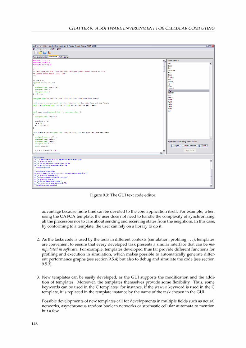
CHAPTER 9. A SOFTWARE ENVIRONMENT FOR CELLULAR COMPUTING

Figure 9.3: The GUI text code editor.

advantage because more time can be devoted to the core application itself. For example, whenusing the CAFCA template, the user does not need to handle the complexity of synchronizingall the processors nor to care about sending and receiving states from the neighbors. In this case,by conforming to a template, the user can rely on a library to do it.

2. As the tasks code is used by the tools in different contexts (simulation, profiling, . . . ), templatesare convenient to ensure that every developed task presents a similar interface that can be ma-nipulated in software. For example, templates developed thus far provide different functions forprofiling and execution in simulation, which makes possible to automatically generate differ-ent performance graphs (see section 9.5.4) but also to debug and simulate the code (see section9.5.3).

3. New templates can be easily developed, as the GUI supports the modification and the addi-tion of templates. Moreover, the templates themselves provide some flexibility. Thus, somekeywords can be used in the C templates: for instance, if the #TASK keyword is used in the Ctemplate, it is replaced in the template instance by the name of the task chosen in the GUI.

Possible developments of new templates call for developments in multiple fields such as neuralnetworks, asynchronous random boolean networks or stochastic cellular automata to mentionbut a few.

148

9.5. TASK PROGRAMMING TOOLS

9.5.2 Task compilation

The second tool was motivated by the observation that, during the development of a program, thecompilation process is always a tedious and time-consuming task. To reduce this time, the GUI pro-poses a single button to compile the tasks programs, which calls a compilation script for the task itself.Every time a new task is created, a dedicated compilation script is generated from a script template toinclude all the requirements of the framework (libraries, compiler flags, etc.) but also so that the usercan change, if required, the compilation script of the task.

In its current state, the compilation process can create two types of executable files: a version fora desktop computer that can be used for simulation (see section 9.5.3) or a version for a dedicatedhardware platform, such as the ULYSSE processor. The output of the compilation process, reportingpotential compilation errors and warnings, is displayed directly in the GUI (shown in the bottom partof Figure 9.3, page 148).

Note that, because the GUI is multi-platform, so are the compilation scripts. For this reason, thesescripts are written in a shell scripting language, in our case bash, that can be run under the majorexisting operating systems.

9.5.3 Task simulation

The third type of tool is related to the need of checking the functionality of the code early in the designprocess even though the application is still incomplete.

Because the tasks are independent in stream computing, there exists the opportunity to simulateand debug them separately. Thus, once the task has been written and successfully compiled, the usercan easily verify that the newly-created task behaves as predicted by simulating it with proper inputs.

As maintaining two different versions of the code, one aimed at simulation and one for execution,would be a waste of time and resources, we introduced in the templates the possibility to generatesmall modifications to account for the differences between the code simulated on a PC and on a differ-ent platform. Thus, a flag in the template can be set during the compilation process to switch betweendifferent main() functions. With this flag, even though the code can start in different functions, thecomputational part of the tasks remains identical for the different versions, the template taking careof calling it according to the situation.

Thanks to the introduction of this mechanism and the execution of the code on a desktop PC, theuser can generate, according to his or her preferences, test vectors for the task, assert the code atdifferent locations, etc. This way, checking the task program functionality is simplified, as the outputinformation of the tasks can be directly displayed in the GUI to verify their proper operation.

9.5.4 Task profiling

The fourth tool finds its roots in the fact that, since some tasks may require specific performanceconstraints, it might prove important to evaluate their most computationally-intensive parts. Thus,we included in the code templates, as well as in the GUI, adequate support to simplify this task.

Using the same methods used for task simulation, a template can contain a dedicated function tobe filled so that the performance of a task can be estimated. It consists of calling a sufficient number oftimes the compute() function of the task so that the code can be annotated with timing and profilinginformation.

The annotation itself is performed using a standard profiler, called gprof 5 [Graham 82,Graham 04].To reduce the inaccuracies inherent to the fact that gprof is using sampling techniques to measurethe time spent in each function, the profiling of the task is done several times before the results areaveraged. Thus, the output of this profiler gives us estimates about:

• the total time of execution;

• the number of times each function has been called;

5This acronym stands for the Gnu PROFiler.

149

CHAPTER 9. A SOFTWARE ENVIRONMENT FOR CELLULAR COMPUTING

• the percentage of the total running time of the program used by each function;

• the number of seconds accounted for by each function;

• the average number of milliseconds spent in each profiled function per call;

• the average number of milliseconds spent in each profiled function and its descendants per call.

(a) Circular tree graph (b) Treemap representation

Figure 9.4: Profiling graphs of a task.

Using the code annotated with the profile information, the GUI can then automatically creategraphs such as the ones shown in Figure 9.4. This representation of profiling, inspired from tools suchas Valgrind [Nethercote 04, Nethercote 06], proposes two distinct views to depict in which functionsthe most time is spent.

The treemap technique [Shneiderman 92], shown on the right of the figure, has the advantage ofproviding a good overview of the program time repartition whereas the circular tree graph (left sideof the figure) presents the call graph6 of the program, with each function being represented by a circlewhose size is proportional to the time spent in the function.

In the example depicted in Figure 9.4, which represents the profile graph of the AES encryptionalgorithm [Daemen 02], it can be seen that the MixColumns() function accounts for roughly 52 per-cent of the total execution time. This fact is shown by a circle area about two times larger than theShiftRows() circle area (23 percent) in the tree graph. Similarly, the area of the function in the treemap is also two times larger. One can also very rapidly distinguish that the AddRoundKey() functionis comparable, in terms of execution time, to the keyexp_round() function.

One aim of this profiling tool was to provide a simple and streamlined way to access performanceinformation so that users can optimize their programs, if required, without needing to know how toset up a software toolchain for that purpose. Moreover, it provides a convenient way to compare twoimplementations to choose the most performant one.

Another goal of the profiling of task programs is to provide to the software framework an estima-tion of the complexity of the tasks, an information that will be important in section 9.6.2 where graphexecution will be simulated using that timing estimation.

6Note that the call graph, i.e. the representation of the program as a tree, is generated by the gprof tool and extracted to bedisplayed in the GUI.

150

9.6. TASK GRAPH PROGRAMMING

If, in our case, that estimation is performed on a desktop PC for simplicity reasons, nothing pre-vents the implementation of a more complex toolchain to profile the tasks on different hardwaresetups and under different conditions.

9.5.5 Task library

When the tasks’ code has been written, optimized and checked with the aforementioned tools, thetasks are stored in a library that collects every realized task so that each kernel function can be madeavailable in different sections of the GUI program for a quick selection.

This library stores in a central directory all the tasks code and related scripts, which provides aconvenient way to retrieve or change the different kernel functions.

9.6 Task graph programming

In the previous section we presented how the development of the kernel functions was simplifiedwithin the GUI thanks to a variety of design tools. Following the same methodology, we will examinenow how the same ideas can be applied to intuitively build and simulate complete application graphsbuilt with these kernel functions.

For the sake of simplicity, both construction and simulation of graphs are presented within a singlewindow, which allows not only to create graphs but also to explore, in a very intuitive way, howdifferent input conditions influence the dynamic evolution of a graph in simulation. More precisely,the GUI proposes three different tools for graphs:

• A graph creator, for editing the graphs.

• A timing simulator, which is used to explore the dynamics of graph execution based only on thetiming information of the tasks.

• A parallel simulator, where the complete graph behavior is simulated with tasks running in par-allel on a desktop computer.

Let us now discuss first the graph creator module before examining two different simulation mod-ules (section 9.6.2 and 9.6.3).

9.6.1 The graph editor

The graph creator and editor module of the GUI is shown in Figure 9.5, the main window containingthe graph. This latter can be interactively edited with mouse operations to add and remove vertices,connect them with edges, etc. The different tasks that can be instantiated can be chosen from a list,shown in the top right-end corner of the figure, containing the task library.

To help the user distinguish the topology of cluttered graphs, hovering the mouse over a taskhighlights with different colors the nodes that are connected to it (see the sink node in Figure 9.5a).For the same reason, different layout algorithms can be applied – statically or dynamically – to thegraph so that it is displayed in an aesthetically pleasing way.

For instance, Figure 9.5b shows the application of a dynamic spring layout algorithm that uses aphysical model so that the vertices of the graph repel and the edges between the nodes act as springs,a configuration that makes the graph react when nodes are dragged for example. The different con-figuration parameters of the layout algorithms, such as in this case the default length of the springs,can be seen on the right-hand side of the picture.

Once the editing process is complete, the generated graph can then be saved as a GXL file, astandard file format using the GraphML (XML based) syntax [Brandes 01] for graphs. Using thisformat has the advantage that the graph can be retrieved in another session but also that it can beused in different graph tools without conversion.

151

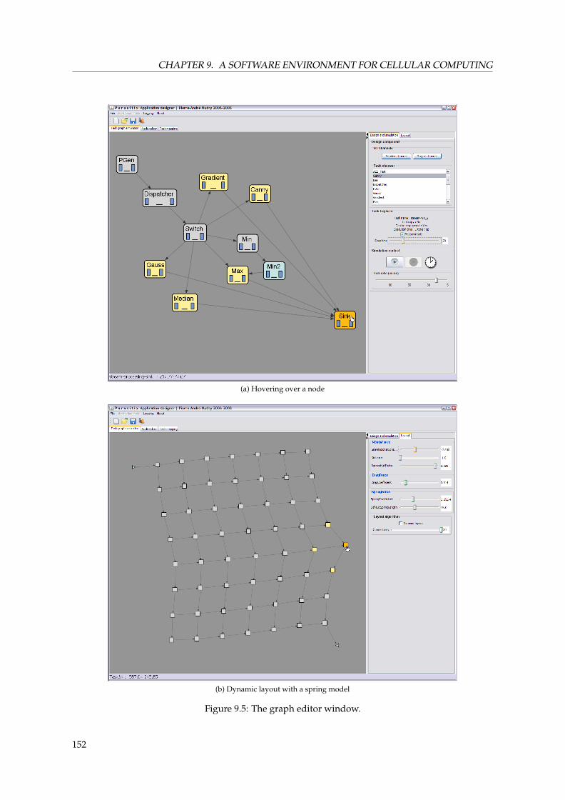
CHAPTER 9. A SOFTWARE ENVIRONMENT FOR CELLULAR COMPUTING

(a) Hovering over a node

(b) Dynamic layout with a spring model

Figure 9.5: The graph editor window.

152

9.6. TASK GRAPH PROGRAMMING

9.6.2 Timing simulation

The first tool to analyze the dynamics of applications proposes to explore the behavior of the graphsbased on the timing information of the tasks, which has been extracted during their profiling. Thissimulation notably enables the user to see the impact of different input scenarios on the graph. Thesescenarios can be chosen by selecting different input channels, i.e. components that generate differenttypes of data at a certain rate. Thus, different input channels were developed using for examplean uniform rate with random data, with data generated following a normal law, etc. More can beimplemented by adding appropriate Java classes.

Figure 9.6: A timing simulation in the GUI.

Bottleneck identification

The second application of these scenarios in a simulation allows to easily identify bottlenecks in theapplication. As shown in Figure 9.6, the tasks can be displayed with three vertical bars that represent,from left to right, the input FIFO level of the task, its load7 and the output FIFO level. In addition,each task can also change the filling color of its background, using different shades to represent theload.

These graphical indications, which are completely flexible because they can be extended to differ-ent models, allow to intuitively identify the presence of “hot-spots” within the application. Moreover, ifrealistic scenarios are used, it also becomes possible to refine the splitting of the graph according tothat information. Finally, it is also possible to plot in real-time the log of different task parameters andsave this information.

7As time is discrete within the simulator, we use the notion of “ticks” represent that a time slot has passed. The load of atask is defined as the ratio of non-idle ticks over a given period.

153

CHAPTER 9. A SOFTWARE ENVIRONMENT FOR CELLULAR COMPUTING

Overall, the animated features of the GUI give a visual feedback to the designer that provides agood insight of the dynamic, global behavior of the application by representing congestions, idlenessand other measures with colors and animations. Thus, it becomes possible to visually represent thepotential problems of a parallel application in ways that are normally difficult or that can be intuitivelymisleading.

Limits

One disadvantage of this timing simulation is that, as it relies heavily on estimates, its quality and itsmatch to reality depends on these estimates and on the model. However, because simulation can beperformed very quickly but also because the simulation model can be improved to take into accountdifferent parameters so that the desired complexity level is attained, this remains a valuable tool thatwill be reused in the next chapter to examine a task replication algorithm (see chapter 10).

9.6.3 Parallel simulation

If the dynamic simulation proposes to focus on the timing characteristics of the graph, the parallel sim-ulation module proposes a way to execute the application code on a distributed environment runningon PC before instantiating it on the target hardware.

In this distributed simulation, each task code is executed in a dedicated thread that can commu-nicate with the other tasks as if they were running in the final hardware, with the notable differencethat here the FIFO-based communication is simulated transparently in the environment by TCP/IPsockets. Thus, from the tasks’ perspective, the code executed is the same as the one on the final hard-ware, all the functionalities provided by the framework libraries, such as the functions to retrieve theFIFO levels, being also simulated.

With this setup, it is possible to run and verify the application in a controlled execution environ-ment which provides debugging functionalities (consoles, breakpoints and step-by-step execution)that the real hardware can not match in its current state.

Receiverthread

Senderthread

Command thread

Task threadcomputation()

Task DLL

Receiverthread

Senderthread

Command thread

Task threadcomputation()

Task DLL

Receiverthread

Senderthread

Command thread

Task threadcomputation()

Task DLL

Java server

Receiverthread

Senderthread

Command thread

Simulation hostlaunchTask()

createTask()

GUI interactions

TCP/IP link

JNI call

Java call

C communication thread

C computation thread

Java thread

Figure 9.7: The parallel simulation environment showing the simulation of three tasks.

From an implementation point of view, this simulation environment is composed of multiple con-current Java and C components which are presented in Figure 9.7. In this schematic, which representsa graph of three tasks in series (see bottom of the figure), each box containing text represents a distinct

154

9.6. TASK GRAPH PROGRAMMING

thread running either in C or Java and its connections with other boxes depict its interactions with theother components.

Starting from a task graph described in the GUI, it is then possible to effectively execute the appli-cation by simulating each task in a parallel thread, also reusing the same C code. A simulation sessionon a PC follows the following procedure:

• A Java server thread is generated to fulfill three different roles:

1. interact with the GUI (and the user);2. ask for tasks to be created or removed;3. communicate with the tasks.

The first role is easily explained by the fact that this server is tightly coupled with the GUIapplication, the user being able to interact with the simulation in real time, which also explainsthe second role of this server.

The communication with the tasks is supported by three different threads, one for receivingapplication data, one for sending data to the application and a last one for passing commandmessages to the tasks. This last category includes special messages which can be used to re-trieve the status of a task (load, FIFO status, . . . ) or to dynamically change the topology of theapplication.

• A Java thread (SimulationHost), triggered by a task creation request by the server, dynamicallyloads the tasks’ C code (which for this phase is compiled as a dynamically-linked library) usinga Java Native Interface (JNI) call8.

• Each time a C task is loaded, it creates two additional threads9 to simulate the FIFOs presentin the hardware interfaces so that the behavior of the task running in a desktop environment issimilar to the behavior in hardware. Each of these communication threads use TCP/IP socketsto communicate from task to task, even though solutions other than FIFO communication orTCP/IP could also be implemented if required. However, the flexibility of TCP/IP allows torun the parallel tasks on different machines if necessary. Finally, for each task loaded, a fourththread is created to react to the commands sent by the Java server.

9.6.4 Tasks placement

The placement of the tasks takes as an input the task graph and a processor graph that contains thetopology of the target hardware to produce as an output a placement of the tasks onto the processors.

At the time of writing, a single type of processor graph has been written, based on the hardwarestructure of the CONFETTI platform, even though everything is planned in the software GUI to easilyintegrate different types of graphs. Also, we only examined with tasks placement the situation inwhich each processor can run at most a single task. The motivation of this decision resides in the lackof a timer interrupt in the ULYSSE processor (see section 2.6.2, page 20) which hinders implementationof a multitasked environment. When used with the CONFETTI platform, the placer module displays(Figure 9.8) the actual topology of the processors as a grid, which helps the user understand theinfluence of the relative placement of the tasks.

For instance, it is relatively obvious that a placement such as the one presented in Figure 9.8apresents several disadvantages when compared to Figure 9.8b. This fact can be rapidly graspedthanks to graphical hints such as the overlapping edges or the fact that the edges are not horizon-tal or vertical, which signifies that routing will have to be done through multiple elements.

Even if we did not investigate or implement the automatic placement of tasks in this work due toa lack of time, this would be an interesting research opportunity that could leverage on an abundantliterature on the subject, such as [Aguilar 97, Bouvry 94].

8JNI is used to call C code within a Java application, see [Liang 99].9All the C threads are created using POSIX threads so that they are compatible with the Linux operating system as well as

with Windows.

155

CHAPTER 9. A SOFTWARE ENVIRONMENT FOR CELLULAR COMPUTING

(a) Bad placement

(b) Good placement

Figure 9.8: The GUI placement module.

156

9.7. CONCLUSION

9.6.5 Graph compilation

Once the application graph is complete and the placement of tasks done, the graph can then be com-piled, i.e. translated into an adequate format to be downloaded to the hardware target. To make thisprocess as extensible as possible, a shell script language is used once again. In the case CONFETTI isused as the hardware target for the graph, the procedure contains the following steps:

1. Each task is compiled for the ULYSSE processor, which is done by calling the makefile of each taskwith a flag indicating the executable type.

2. On demand, a USB interface program is called to download the processors’ code to the CON-FETTI platform according to the mapping information gathered from the placer tool.

The whole procedure of graph compilation is automated and can be launched from the GUI, whichmakes sense as each alteration of the tasks placement or of the tasks’ code require a new graph com-pilation.

9.6.6 Graph execution

To replicate the presence in CONFETTI of a command channel as used in simulation, it is also possibleto send commands to the tasks executed in the real platform thanks to a dedicated program, whoserole is basically to translate messages sent with the TCP/IP protocol to USB commands that are thenrouted to the CONFETTI platform. With this mechanism, the whole hardware platform can be accessedfrom any device capable of TCP/IP connectivity.

An example of the commands that are implemented and that can be sent or received from CON-FETTI – or any other hardware with an adequate protocol – are for instance requesting the status ofa particular processor’s input or output FIFO, retrieving the load of a processor, requesting a proces-sor replication or migration to another location, etc. In fact, any command can be imagined as theirimplementation only requires to add functions to the MERCURY API library presented in section 8.5.

9.7 Conclusion

The GUI program that was demonstrated in this chapter constitutes a valuable tool in providingusers a system view powerful enough to be able to manage the complexity of parallel systems whileremaining simple enough for novices to access complex hardware.

In addition, we also discussed in this chapter how, in order for bio-inspired concepts to be acceptedas valuable tools for the design and use of digital computing systems, they will have to be tested andverified on complex real-world applications. The experimental setups associated with research inthis field, however, are often of limited use in this context because they remain either too specific ortoo difficult to use beyond the proof-of-concept stage. By guiding the user through different explicitand intuitive modules in the GUI the process of developing bio-inspired applications such as cellularautomata with our approach becomes a matter of hours or minutes.

When compared with a traditional approach, such as the one used for the BioWall where onlyhardware programmability was possible, this considerable reduction in design time constitutes a ma-jor step forward. Moreover, not only can the platform be easily used but also the shift from a completehardware approach towards a more software-oriented one allows far more flexibility while preservingthe capability of accessing the low-level hardware if necessary. A possible target for further researchwould be to exploit this flexibility to an even greater degree, notably by directly integrating codesignmodules for the processor in the GUI, for example to take advantage of novel hardware-softwarecodesign techniques, such as UML, as presented in the work of Bocchio et al. (see, for example, [Boc-chio 07, Riccobene 05]).

In the next chapter, we will see how this mixed software/hardware approach is not restrictedto bio-inspired computations but can also be used to accelerate standard algorithms, such as AESencryption, thanks to the self-scaling stream processing paradigm.

157

Bibliography

[Aguilar 97] Jose Aguilar & Erol Gelenbe. Task assignment and transaction clustering heuristics fordistributed systems. Information Sciences, vol. 97, pages 199–219, 1997.

[Ahmad 99] Ishfaq Ahmad & Yu-Kwong Kwok. On Parallelizing the Multiprocessor SchedulingProblem. IEEE Transactions on Parallel and Distributed Systems, vol. 10, no. 4, pages414–432, 1999.

[Bocchio 07] Sara Bocchio, Elvinia Riccobene, Alberto Rosti & Patrizzia Scandurra. Advances inDesign and Specification Languages for Embedded Systems, chapter "A Model-drivenco-design flow for Embedded Systems". Springer, 2007.

[Bouvry 94] Pascal Bouvry, J.-M. Geib & D. Trystram. Analyse et conception d’algorithmes parallèles.Hermes, April 1994.

[Brandes 01] Ulrik Brandes, Markus Eiglsperger, Ivan Herman, Michael Himsolt & M. Scott Mar-shall. GraphML Progress Report, Structural Layer Proposal. In Proceedings of the 9thInternational Symposium on Graph Drawing (GD’2001), pages 501–512, Heidel-berg, 2001. Springer Verlag.

[Buck 04] Ian Buck, Tim Foley, Daniel Horn, Jeremy Sugerman, Kayvon Fatahalian, MikeHouston & Pat Hanrahan. Brook for GPUs: stream computing on graphics hardware. InACM SIGGRAPH 2004 Papers, pages 777–786. ACM, 2004.

[Daemen 02] Joan Daemen & Vincent Rijmen. The Design of Rijndael: AES – the Advanced Encryp-tion Standard. Springer, 2002.

[Dally 03] William J. Dally, Francois Labonte, Abhishek Das, Patrick Hanrahan, Jung-Ho Ahn,Jayanth Gummaraju, Mattan Erez, Nuwan Jayasena, Ian Buck, Timothy J. Knight &Ujval J. Kapasi. Merrimac: Supercomputing with Streams. In SC ’03: Proceedings ofthe 2003 ACM/IEEE conference on Supercomputing, page 35, Washington, USA,2003. IEEE Computer Society.

[Engler 95] D. R. Engler, M. F. Kaashoek & Jr. J. O’Toole. Exokernel: an operating system archi-tecture for application-level resource management. SIGOPS Operating Systems Review,vol. 29, no. 5, pages 251–266, 1995.

[Fernando 03] Randima Fernando & Mark J. Kilgard. The Cg Tutorial: The Definitive Guide to Pro-grammable Real-Time Graphics. Addison-Wesley, Boston, MA, USA, 2003.

[Gajski 82] D. D. Gajski, D. A. Padua, D. J. Kuck & R. H. Kuhn. A Second Opinion on Data FlowMachines and Languages. Computer, vol. 15, no. 2, pages 58–69, 1982.

[Garey 79] M. R. Garey & D. S. Johnson. Computers and Intractability : A Guide to the Theory ofNP-Completeness. Series of Books in the Mathematical Sciences. W.H. Freeman &Company, January 1979.

159

BIBLIOGRAPHY

[Ghuloum 07] Anwar Ghuloum. Ct: channelling NeSL and SISAL in C++. In CUFP ’07: Proceedingsof the 4th ACM SIGPLAN workshop on Commercial users of functional program-ming, pages 1–3, New York, USA, 2007. ACM.

[Gordon 06] Michael I. Gordon, William Thies & Saman Amarasinghe. Exploiting coarse-grainedtask, data, and pipeline parallelism in stream programs. In ASPLOS-XII: Proceedingsof the 12th International Conference on Architectural support for programminglanguages and operating systems, pages 151–162, New York, USA, 2006. ACM.

[Graham 82] Susan L. Graham, Peter B. Kessler & Marshall K. Mckusick. Gprof: A call graphexecution profiler. In SIGPLAN ’82: Proceedings of the 1982 SIGPLAN symposiumon Compiler construction, pages 120–126, New York, USA, 1982. ACM.

[Graham 04] Susan L. Graham, Peter B. Kessler & Marshall K. McKusick. Gprof: A call graphexecution profiler. SIGPLAN Notices, vol. 39, no. 4, pages 49–57, 2004.

[Greensted 07] A.J. Greensted & A.M. Tyrrell. RISA: A Hardware Platform for Evolutionary Design.In Proc. IEEE Workshop on Evolvable and Adaptive Hardware (WEAH07), pages1–7, Honolulu, Hawaii, April 2007.

[Heer 05] Jeffrey Heer, Stuart K. Card & James A. Landay. Prefuse: a toolkit for interactiveinformation visualization. In Proceeding of the SIGCHI conference on Human factorsin computing systems (CHI ’05), pages 421–430, New York, 2005. ACM Press.

[Hutton 07] Graham Hutton. Programming in Haskell. Cambridge University Press, January2007.

[Iverson 62] Kenneth E. Iverson. A Programming Language. John Wiley & Sons, 1962.

[Jerraya 05] Ahmed Jerraya & Wayne Wolf. Multiprocessor Systems-on-Chips. Morgan Kaufmann,San Francisco, California, 2005.

[Jerraya 06] Ahmed Jerraya, Aimen Bouchhima & Frédéric Pétrot. Programming models and HW-SW interfaces abstraction for multi-processor SoC. In Proceedings of the 43rd annualconference on Design automation (DAC’06), pages 280–285, New York, USA, 2006.ACM.

[Johnston 04] Wesley M. Johnston, J. R. Paul Hanna & Richard J. Millar. Advances in dataflowprogramming languages. ACM Computing Survey, vol. 36, no. 1, pages 1–34, 2004.

[Kahn 74] G. Kahn. The Semantics of a Simple Language for Parallel Programming. In J. L. Rosen-feld, editor, Proceedings of the IFIP Congress on Information Processing, pages471–475. North-Holland, New York, USA, 1974.

[Kapasi 02] Ujval Kapasi, William J. Dally, Scott Rixner, John D. Owens & Brucek Khailany. TheImagine Stream Processor. In Proceedings of the IEEE International Conference onComputer Design, pages 282–288, September 2002.

[Lewis 90] T.G. Lewis, H. El-Rewini, J. Chu, P. Fortner & W. Su. Task Grapher: A Tool for Schedul-ing Parallel Program Tasks. Proceedings of the Fifth Distributed Memory ComputingConference, vol. 2, pages 1171–1178, April 1990.

[Liang 99] Sheng Liang. Java Native Interface: Programmer’s Guide and Specification. PrenticeHall, 1999.

[Nesbit 08] K.J. Nesbit, M. Moreto, F.J. Cazorla, A. Ramirez, M. Valero & J.E. Smith. MulticoreResource Management. IEEE Micro, vol. 28, no. 3, pages 6–16, May-June 2008.

[Nethercote 04] Nicholas Nethercote. Dynamic Binary Analysis and Instrumentation. PhD thesis, Uni-versity of Cambridge, November 2004.

160

BIBLIOGRAPHY

[Nethercote 06] N. Nethercote, R. Walsh & J. Fitzhardinge. Building Workload Characterization Toolswith Valgrind. In Proceedingso of the IEEE International Symposium on WorkloadCharacterization, pages 2–2, 2006.

[Peterson 81] James Lyle Peterson. Petri Net Theory and the Modeling of Systems. Prentice Hall PTR,Upper Saddle River, NJ, USA, 1981.

[Pham 06] D.C Pham, T. Aipperspach & D. Boerstler et al. Overview of the architecture, circuitdesign, and physical implementation of a first-generation CELL processor. IEEE Solid-State Circuits, vol. 41, no. 1, pages 179–196, 2006.

[Riccobene 05] Elvinia Riccobene, Patrizzia Scandurra, Alberto Rosti & Sara Bocchio. A SoC De-sign Methodology Involving a UML 2.0 Profile for SystemC. In Proceedings of theconference on Design, Automation and Test in Europe (DATE’05), pages 704–709,Washington, DC, USA, 2005. IEEE Computer Society.

[Sarkar 89] Vivek Sarkar. Partioning and Scheduling Parallel Programs for Multiprocessors. Re-search Monographs in Parallel and Distributed Computing. Pitman, London andthe MIT Press, Cambridge, MA, 1989.

[Shneiderman 92] Ben Shneiderman. Tree visualization with tree-maps: 2-d space-filling approach. ACMTransactions on Graphics, vol. 11, no. 1, pages 92–99, 1992.

[Snir 96] Marc Snir, Steve Otto, Steven Huss-Lederman, David Walker & Jack Dongarra.MPI: The Complete Reference. Scientific and Engineering Computation Series. MITPress, February 1996.

[Taylor 02] Michael Bedford Taylor, Jason Kim, Jason Miller, David Wentzlaff, Fae Ghodrat,Ben Greenwald, Henry Hoffman, Paul Johnson, Jae-Wook Lee, Walter Lee, AlbertMa, Arvind Saraf, Mark Seneski, Nathan Shnidman, Volker Strumpen, Matt Frank,Saman Amarasinghe & Anant Agarwal. The Raw Microprocessor: A ComputationalFabric for Software Circuits and General-Purpose Programs. IEEE Micro, vol. 22, no. 2,pages 25–35, 2002.

[Tempesti 01] Gianluca Tempesti, Daniel Mange, André Stauffer & Christof Teuscher. The BioWall:an electronic tissue for prototyping bio-inspired systems. In Proceedings of the 3rdNasa/DoD Workshop on Evolvable Hardware, pages 185–192, Long Beach, Cali-fornia, July 2001. IEEE Computer Society.

[Thies 02] William Thies, Michal Karczmarek & Saman P. Amarasinghe. StreamIt: A Languagefor Streaming Applications. In Proceedings of the 11th International Conferenceon Compiler Construction (CC’02), pages 179–196, London, UK, 2002. Springer-Verlag.

[Thoma 04] Yann Thoma, Gianluca Tempesti, Eduardo Sanchez & J.-M. Moreno Arostegui. PO-Etic: An Electronic Tissue for Bio-Inspired Cellular Applications. BioSystems, vol. 74,pages 191–200, August 2004.

[Upegui 07] Andres Upegui, Yann Thoma, Eduardo Sanchez, Andres Perez-Uribe, Juan-Manuel Moreno Arostegui & Jordi Madrenas. The Perplexus bio-inspired reconfig-urable circuit. In Proceedings of the 2nd NASA/ESA Conference on Adaptive Hard-ware and Systems (AHS07), pages 600–605, Washington, USA, 2007.

[van der Wolf 04] Pieter van der Wolf, Erwin de Kock, Tomas Henriksson, Wido Kruijtzer & GerbenEssink. Design and programming of embedded multiprocessors: an interface-centric ap-proach. In Proceedings of the 2nd IEEE/ACM/IFIP international conference onHardware/software codesign and system synthesis (CODES+ISSS ’04), pages 206–217, New York, USA, 2004. ACM.

161

Chapter 10

Self-scaling stream processing

“The future has already arrived.It’s just not evenly distributed yet.”

WILLIAM GIBSON

THE EVER-INCREASING demand in processing power imposed, for example, by the popularity ofhigh-definition media, has revamped interest in multiprocessor systems, which can provide sig-

nificant advantages in terms of testability or performance scaling; criteria such as time-to-marketor lower non-recurrent engineering costs thanks to design reuse are also contributing to this trend.Given the difficulty of devising novel high-performance processor microarchitectures, multiproces-sor systems provide another way to exploit the growing number of transistors on a chip by re-usingan identical design several times over.

Unfortunately, decades of compiler research have not yet succeeded in providing an automatedway to exploit the full potential of parallelism. Consequently, multi-threaded applications are stillmostly designed by hand and require strong parallel coding skills, still scarce in the programmingcommunity. One solution that has been proposed to speed up the development of such systemsis to rely on pipeline parallelism, where computation is divided into several stages that process datalocally before forwarding them to the next stage. This kind of parallelism, which was introducedin the previous chapter, possesses several advantages, such as good data locality and the fact that,in opposition to task parallelism, data sharing and synchronization are handled in such a way thatmost of the typical problems of concurrent programming, such as race conditions and deadlocks, areavoided.

10.1 Introduction and motivations

Obviously, several classes of problems solvable in parallel can be tackled more easily by the use ofadequate programming paradigms: parallelism at the task level can thus be handled by threads ordata-level parallelism by SIMD instructions. However, such paradigms are often of little help whenscarce and specific resources have to be used, which is often the case with multiprocessor embeddedsystems. In this context, which often imposes strict cost and performance requirements, completehand design of applications remains common. Such a design follows an iterative process: the ap-plication is split into different tasks or threads which are then mapped to different processors. Thecomplete system is then profiled to determine if it fulfills all timing requirements and the procedureis repeated until all criteria are met. This time-consuming process has to be repeated for every newapplication and the quality of the outcome mainly depends on designer experience.

Several efforts to achieve automatic extraction of pipeline parallelism from programs have beenattempted, either based on fine-grained (instruction-level) [Ottoni 05] or coarse-grained (function-level) [Dai 05] techniques. Other methods such as code annotation [Thies 07] rely on programmerexpertise to extract the underlying parallelism. In addition to pipeline parallelism, task migration in

163

CHAPTER 10. SELF-SCALING STREAM PROCESSING

multiprocessor systems on chip (MPSoC) has been the focus of some interest recently [Bertozzi 06,Ngouanga 06,Pittau 07] and has positioned itself as a partial solution to perform dynamic load distri-bution in academic and commercial systems.

In this chapter, we aim at demonstrating a new technique that combines the different approacheswhile offering the system designer an interesting alternative to completely hand-tailored systems inthe context of coarse-grained streaming applications, a class of problems characterized by a flow of dataon which computation is carried out sequentially [Bridges 08, Buck 04].

Our approach leverages the software GUI presented previously and requires the programmer todivide computation into a graph of independent tasks, which are then mapped onto computing nodes.The main novelty of our solution – largely independent of the nature of the processing nodes that canrange from the elements of a MPSoC to a grid of computers – resides in the dynamic and distributedexecution of an algorithm that enables tasks to replicate on demand. This replication can be initiatedaccording to various criteria, such as CPU load or buffer occupation, without requiring the use of acentralized manager, and allows an application to grow and self-organize.

It should be pointed out from the outset that this technique is based on the strong assumptionthat computing resources are available in large quantities, since it does not hesitate to use resourcesthat are not always strictly necessary. As such, its primary advantage is not optimal performance butthe fact that it can used as a dynamic, distributed and scalable load distribution technique which isable not only to quickly respond to workload changes but also to act as a simple resource allocationheuristic in massively parallel embedded systems.

To show the value of the approach, we applied it to a 36-processor system implemented on ascalable mesh of FPGAs for two different case studies: AES encryption and MJPEG compression. Inthe first case, we obtained up to a ten-fold speedup compared to a static implementation and, in thesecond case, a throughput multiplication of 11.

This chapter is organized as follows: in the next section, we formulate the problem in terms of a dis-tributed replication algorithm. The following section is dedicated to the design and implementationof the algorithm itself. Thereafter, we present some experimental results which show the efficiency ofour approach. Finally, section 10.7 concludes this chapter and introduces future work.

10.2 Self-scaling stream processing

One of the objectives pursued by our software/hardware framework is to provide the user with asimple and automatic method to use parallel systems. As mentioned earlier, pipeline parallelism canbe used to increase application performance. Stream processing is an instance of this model in whichcomputation is transformed into a sequence of independent kernel functions sequentially applied to adata stream. If these functions can run simultaneously, an execution pipeline is formed.

An important advantage of stream processing is the ease with which it can be adapted to run onhighly-parallel computer systems. Thanks to independent kernel functions, concurrency issues aregreatly reduced: no data sharing and synchronization are required, except for the passing of streamdata between successive pipeline stages. Thus, kernel functions can be separated to run on different,separate computational nodes – be they threads, cores, or CPUs – as long as a way to convey databetween them exists. This ability to run separately can lead to an enhancement of the static DAGmodel with the possibility to dynamically create and/or migrate tasks as we will see now.

10.2.1 Task migration

Task migration consists of changing the mapping of tasks to nodes during the execution of the pro-gram. According to [Bouvry 94], this migration can occur in the middle of a computation, an optionwhich requires checkpointing mechanisms, or only at certain locations, such as function boundaries. Inthis work, we will consider this latter option only for the sake of simplicity.

A typical case where migration could occur is when two tasks are executed on a single processorand one of them is migrated to another processor to distribute the load. Another situation that canbenefit from task migration is when a different placement of the tasks within the parallel platform

164

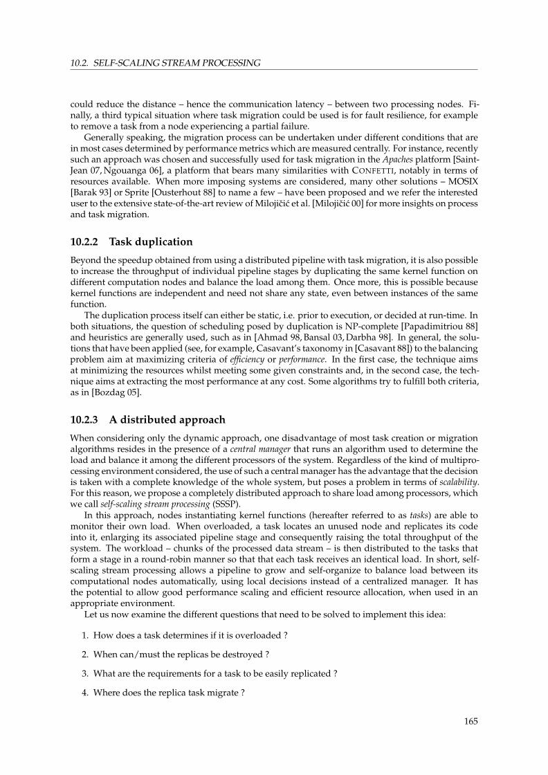
10.2. SELF-SCALING STREAM PROCESSING

could reduce the distance – hence the communication latency – between two processing nodes. Fi-nally, a third typical situation where task migration could be used is for fault resilience, for exampleto remove a task from a node experiencing a partial failure.

Generally speaking, the migration process can be undertaken under different conditions that arein most cases determined by performance metrics which are measured centrally. For instance, recentlysuch an approach was chosen and successfully used for task migration in the Apaches platform [Saint-Jean 07, Ngouanga 06], a platform that bears many similarities with CONFETTI, notably in terms ofresources available. When more imposing systems are considered, many other solutions – MOSIX[Barak 93] or Sprite [Ousterhout 88] to name a few – have been proposed and we refer the interesteduser to the extensive state-of-the-art review of Milojicic et al. [Milojicic 00] for more insights on processand task migration.

10.2.2 Task duplication

Beyond the speedup obtained from using a distributed pipeline with task migration, it is also possibleto increase the throughput of individual pipeline stages by duplicating the same kernel function ondifferent computation nodes and balance the load among them. Once more, this is possible becausekernel functions are independent and need not share any state, even between instances of the samefunction.

The duplication process itself can either be static, i.e. prior to execution, or decided at run-time. Inboth situations, the question of scheduling posed by duplication is NP-complete [Papadimitriou 88]and heuristics are generally used, such as in [Ahmad 98, Bansal 03, Darbha 98]. In general, the solu-tions that have been applied (see, for example, Casavant’s taxonomy in [Casavant 88]) to the balancingproblem aim at maximizing criteria of efficiency or performance. In the first case, the technique aimsat minimizing the resources whilst meeting some given constraints and, in the second case, the tech-nique aims at extracting the most performance at any cost. Some algorithms try to fulfill both criteria,as in [Bozdag 05].

10.2.3 A distributed approach

When considering only the dynamic approach, one disadvantage of most task creation or migrationalgorithms resides in the presence of a central manager that runs an algorithm used to determine theload and balance it among the different processors of the system. Regardless of the kind of multipro-cessing environment considered, the use of such a central manager has the advantage that the decisionis taken with a complete knowledge of the whole system, but poses a problem in terms of scalability.For this reason, we propose a completely distributed approach to share load among processors, whichwe call self-scaling stream processing (SSSP).

In this approach, nodes instantiating kernel functions (hereafter referred to as tasks) are able tomonitor their own load. When overloaded, a task locates an unused node and replicates its codeinto it, enlarging its associated pipeline stage and consequently raising the total throughput of thesystem. The workload – chunks of the processed data stream – is then distributed to the tasks thatform a stage in a round-robin manner so that that each task receives an identical load. In short, self-scaling stream processing allows a pipeline to grow and self-organize to balance load between itscomputational nodes automatically, using local decisions instead of a centralized manager. It hasthe potential to allow good performance scaling and efficient resource allocation, when used in anappropriate environment.

Let us now examine the different questions that need to be solved to implement this idea:

1. How does a task determines if it is overloaded ?

2. When can/must the replicas be destroyed ?

3. What are the requirements for a task to be easily replicated ?

4. Where does the replica task migrate ?

165

CHAPTER 10. SELF-SCALING STREAM PROCESSING

5. How can the global behavior of the application be maintained with dynamically created anddeleted tasks ?

6. How is global performance affected by the dynamic replication of the tasks?

Answering these questions will be the guiding thread of the remainder of this chapter: the firsttwo questions will be examined in detail in section 10.6, the next three in section 10.4 and, finally, theperformance question will be discussed with various experiments in section 10.5.

10.3 Design

Preliminary remark The graphs presented in this section as well as its organization are based on JulienRuffin’s master thesis [Ruffin 08], and were modified with permission.

With the general aim of the algorithm outlined, we will now focus on the requirements needed toimplement the replication algorithm itself.

First, we need a means to distinguish between the different task roles in the pipeline. This isachieved by allocating to a given stage of the pipeline a group identifier at initialization. To create thehierarchy present in the pipeline, each cell also receives a list of its successor groups. For each of thesuccessor group ID, the cells keep a list of the members of that group that is updated by notificationmessages broadcast to the entire grid when a node is created or destroyed.

Kernelfunction

Job FIFO

Kernelfunction

Job FIFO

Kernelfunction

Job FIFO

Input job

Job 1 to 2

Output job

Stage / Group 1

Stage / Group 2

Stage / Group 3

Job 2 to 3

Kernelfunction

Job FIFO

Kernelfunction

Job FIFO

Kernelfunction

Job FIFO

Figure 10.1: Sample 3-stage SSSP pipeline with duplicated stage 2 and 3.

With this organization, every time a cell finishes processing a job, it can dispatch the output furtherto its successors using a round-robin scheduling technique. For instance, Figure 10.1 shows a threelevel pipeline with the second stage distributed on three processors and the last stage on two proces-sors. With round-robin scheduling, any incoming packet arriving in stage 1 is forwarded to one of thecells in stage 2 (the exact destination cell changing for each new packet). In the configuration depictedhere, the next packet arriving in stage 1 would then be forwarded in the upper cell of stage 2 (whichis the next in the schedule) before being sent to a cell in stage 3 that depends upon the round-robinstate of the sender cell in stage 2.

10.3.1 Message types and interface

New message types have been added on top of the MERCURY API to account for the needs of thiskind of pipeline organization. These messages are independent of the type of MERCURY packet in

166

10.3. DESIGN

which they are encapsulated, i.e. they can be used in broadcast or one-way messages without anydifference. Four different message types can be distinguished:

1. Jobs. This first message type contains job data that the task has to work on. The header of themessage itself contains the sender address, the group ID it is destined to, as well as the payloadlength of the data.

2. Control messages. These messages can be used to request information from the tasks (such astheir load) or to inform them of something. The header of the message contains the senderaddress, a control field that indicates the type of request and an optional payload length.

3. Status messages. This type of message is used to reply to a control message. It uses the same typeof header as these latter.

4. Boot message. Message type received to start the task and also to provide run-time information.For instance, the organization of the pipeline is not fixed at compile time but is dynamic. Thus,the function graph can be constructed at runtime in the system with appropriate messages thatindicate to each group its successors, which allows additional flexibility.

10.3.2 Program structure

A typical SSSP application contains several subfunctions that handle the different types of processingrequired in the task, namely the handling of the data I/O operations and the computation itself.

Cyclic executive

The structure of SSSP programs, shown in Figure 10.2, is based on a cyclic executive program thatswitches between I/O and computation phases.

A cell must basically execute two types of operations: the first consists in filling the job FIFO withdata coming from the network1 and the second relates to the computing proper.

This kind of setup is relatively common and is generally handled with interrupts triggered by in-coming data and an infinite loop to process the jobs available. However, as we mentioned earlier (seesection 2.6.2, page 20), interrupts are too complex and computationally intensive in single-instructionarchitectures and they were not implemented. Consequently, the implementation of the SSSP algo-rithm within the ULYSSE processor uses polling for I/O operations and static multitasking is obtainedwith cyclic executives, meaning that the processor always executes a single task, as shown in the fol-lowing code:

void cyclic_executive(){while(1){

fill_queue();process_jobs();

}}

Both functions present in the infinite loop run for a defined period of time in their own processingloop and then return, which enables an alternating behavior. To control the duration of each function,both calls use the timer unit present in ULYSSE to check that a certain amount of time has elapsed.

Of course, the disadvantage of this technique is that the duration of each function has to be deter-mined manually, depending on the ratio of communication time versus computation time of particu-lar applications. As such, the implementation of interrupts would be more elegant but, unfortunately,we did not have time to investigate this solution.

1Note that the job FIFO resides in the program memory and is different from the MERCURY FIFO present in hardware.

167

CHAPTER 10. SELF-SCALING STREAM PROCESSING

Try receiving

Gotmessage?

Handle message(if job: enqueue)

Timeout ?

FIFOfull ?

yes no

no no

Process job(send further job)

FIFO empty ?

Timeout ?

Consider replication or retirement

yes yes

yes

no

yes

no

fill_queue()

process_jobs()

Figure 10.2: Cyclic executive graph.

10.3.3 Programmer interface

The programmer’s interface is similar to CAFCA, presented in section 8.6. As a summary of thedifferent functionalities of the SSSP API, the following code depicts the implementation of the identityfunction, which basically forwards a packet to the next pipeline stage without modifying it:

#include "stream-processing-common.h"const int CODE_BORDER = 0;#include "stream/stream.h"

void computation(job ∗j) {stream_output(out_job); // Send the job "as−is" to the next stage .

}

void init () {app_computation = &computation;stream_duplicable = 0; // Set this to set initial dynamic duplicability

}

void main() {stream_init(INJECTION_ADDR, MIN_X, MAX_X, MIN_Y, MAX_Y, &init);stream_main_loop();

}

Listing 10.1: Stream identity function.

168

10.4. THE REPLICATION ALGORITHM

As with CAFCA, the SSSP framework contains functions that ought to be called at initializationto locate the user’s custom initialization function and the computation function. At startup, a call tothe stream_main_loop() functions starts the cyclic executive which in turn periodically calls thecomputation function.

Every kernel computation function must provide a pointer to a job structure, for this data typecontains not only the sender information but also the data to be processed by the function. The useof a pointer enables to change the size of the data payload along the pipeline if required so that thetransmitted packets remain as small as possible.

Once the computation proper is finished, the framework provides the user with a simple function,stream_output(), that can be used to forward the packet to the task’s successor in the pipeline. Itis worth noting here that it is the framework itself, and not the user, that takes care of determiningaddresses by looking up the target in its next-stage member list using a round-robin selection tobalance the load among the successors. If multiple successor groups are present, a similar functionexists to choose among them.

10.4 The replication algorithm

The SSSP model specifies that a task should replicate when overloaded to enable the approach de-scribed in sections 10.1 and 10.2. In the algorithm considered here, a task simply launches the replica-tion process whenever its input FIFO buffer is filled past a certain threshold. However, the range ofpossible alternative criteria imply the existence of different replication policies which we shall discuss insection 10.6. To avoid overgrowth and allow reuse of computation nodes, SSSP tasks also implementa retirement policy similar to the replication policy. Retired tasks stop processing data.

10.4.1 Free cell search algorithm

When replicating, a working SSSP grows by copying its code to free cells, computation nodes whichare initialized empty at startup or retired SSSP tasks.

To find suitable targets for replication, SSSP tasks in CONFETTI keep track of active computationnodes through messages sent from starting-up and retiring tasks, which are broadcast to the entireprocessor grid. This “state table” is built dynamically since the very beginning of the system: everytime a new cell appears in CONFETTI – either by replication or by instantiation – it broadcasts to theentire grid the fact that it is used. A similar mechanism is also present each time a cell is removedfrom the grid. Thus, each node knows exactly the state of each cell of the grid (that busy table is alsocopied in the replication process).

9 10 11 12 13

14

16

18

20 21 22 23 24

15

17

19

1

4

6

2 3

5

87

Figure 10.3: Free cell search algorithm order.

When needed, the free cell search algorithm uses this information to find a suitable replicationtarget, beginning with the eight immediate neighbors of the cell it runs in (the exact order2 is shownin Figure 10.3), then gradually increasing the search perimeter until a free cell is found or it outgrows

2Other search orders are possible, for example to reduce the number of hops between two replica.

169

CHAPTER 10. SELF-SCALING STREAM PROCESSING

the bounds of the processor grid. This local search algorithm is based upon the observation thatcommunication is less susceptible to create congestions in the underlying network by having relatedmessages always go to the same area instead of having messages scattered among different locationson the grid.

For very large computational grids, the scalability of the presented technique could pose a prob-lem, notably in terms of memory required to store the list of the available cells. If scale does becomean issue (which was not the case in our system), many other techniques can of course be applied. Forexample, instead of keeping a list to determine the state of a cell, another solution would have beento implement a query mechanism. However, concerns about the relative slowness of the approach andthe potential issues in terms of concurrency that could appear with such a technique made us preferthe former solution.

10.4.2 The replication function

We will now examine how the replication mechanism is implemented within CONFETTI. As men-tioned earlier in section 8.4.1 (page 127), the ULYSSE processor present in the computation nodes inCONFETTI can be reprogrammed at runtime with a specific message. This is very practical for testing,as the PC interface to the system needs only send such a message to the nodes it wants to reprogramwith the executable code as payload.

In the case of cell replication, the initiating running node wants to copy its code over to another.For efficiency reasons, no separate copy of the code is kept to this end; the sent code has to be extractedfrom the node’s own. When doing so, it is easy to know where the code begins, as it is loaded fromaddress 0. However, determining where in memory code ends and data begins is non-trivial.

CODE_BORDER

bu�ersruntime data

program codelookup tables send

crop

Source memory content

Con�ture messagetype: reprogramdestination: targetlength: &CODE_BORDERpayload: CODE_BORDER

bu�ersruntime data

program codelookup tablesreceive

initialize

program codelookup tables

Destination memory content

Figure 10.4: Summary of CONFITURE code replication (memory contents not to scale).

Copying the entire memory contents is not an option. Currently, the sent code must hold in asingle CONFITURE message, which limits its size to 65534 32-bit words3. Bearing this in mind, astraightforward solution would be to write the code size at a given address at compile-time. Whilepossible, this proves relatively inelegant.

Our attempt at a solution uses existing features to make the compiler and assembler work towardseasily finding code size. It stems from the following observations:

1. The compiler allocates data words for global variables with initial values in declaration order inthe output assembly.

3The maximum size of a MERCURY packet minus one word used for the CONFITURE header extension.

170

10.4. THE REPLICATION ALGORITHM

2. The assembler relocates the aforementioned data words after the code in memory, but beforeglobal variables without initial content.

3. Global variables (including buffers) need not be copied as long as they are all initialized at runtime. What matters is the room allocated to them by the compiler.

This said, the solution, summarized in Figure 10.4, involves declaring a given global constant withan initial value (currently named CODE_BORDER) at the very beginning of the application code (seeListing 10.1 for example). When replicating, the code is taken between address 0 and the address ofthe constant (obtained in C with the &CODE_BORDER expression), then sent. The target’s MERCURYreceiver checks the message type, as declared in the CONFITURE header, and notices it contains code:its DMA unit writes the message payload from address 0 onwards to replace current application code.

All global variables with initial values declared before CODE_BORDER will be part of the replicatedcode. Any global variable declared after it will not see its initial content sent. Special care must betaken to ensure such globals are initialized at runtime. Using this setup, a typical SSSP task replicationtakes between 50 ms and 100 ms.

By modifying the replication function so that it copies its entire memory content, it would alsobe possible to migrate a task completely. However, it would require to implement a checkpointingmechanism (see [Milojicic 00]) to retrieve the location of the PC after migration, which can be donefor example by adding at memory location 0 a jump to the desired PC location.

10.4.3 Startup and replication mechanisms

Now that the question of how replication is performed is answered, let us now examine how it can beused by the SSSP algorithm to copy a cell’s code into a free node. In fact, although code replication isfairly simple, precautions need to be taken in order to keep SSSP nodes in a consistent state. In orderto understand why, it is necessary to briefly explain the boot process of SSSP tasks.

SSSP nodes start up in two phases. First, they are programmed with the task they must imple-ment. Then, they are set up using a boot message to provide up-to-date runtime information, includ-ing pipeline structure and lists of the addresses of the tasks in the next stage of the pipeline. Thesemessages are sent by the PC interface when the SSSP is initialized, or by a replicating task to its target.

The boot message allows major parameters of a SSSP (including pipeline structure) to be changedat initialization without the need to recompile the task code. However, the drawback of this two-phase startup lies in potential concurrency issues when two tasks A and B try to replicate themselvesinto the same free cell C. The worst-case scenario happens when C gets completely reprogrammedand initialized by A, and then right afterwards by B. In this case, other tasks register C as being acopy of both A and B, which is incorrect.

Since in CONFETTI reprogramming is handled in hardware and immediately suspends currently-running program code to replace it with the new code, a task has no way to indicate others the above-mentioned situation is happening. It is thus an issue fairly specific to our platform.

To avoid this issue of concurrent cell reprogramming, a locking mechanism is used, as depicted inFigure 10.5.

A task wanting to replicate itself first sends a replication request message to its target; only whena replication granted message has been received does reprogramming take place. This confirmationis not waited for by the originating task, which continues operating normally. Only free cells grantoverwriting of their code, once. Thus, only the first task from which the request was received willactually send a reprogramming and boot messages. Finally, once a task has been programmed andhas received its boot message, it broadcasts its creation to the entire cell grid. This allows all concernedSSSP tasks to update their address lists, making the newly-created task part of the system. From thereon, it will receive data to process as a member of the pipeline stage it belongs to.

10.4.4 Limiting growth

The described replication algorithm is susceptible to sudden, explosive growth: once a new task iscreated, it takes a certain amount of time for the system to stabilize in its new configuration and

171

CHAPTER 10. SELF-SCALING STREAM PROCESSING

Cell A Cell BFree cell

Cell A(copy)

Request duplication

Proceed with duplication

Update free cell listUpdate target list if needed

Request granted

Request denied (no answer)

Request duplication

[reprogram and reset]

Init

Wait for boot message

Finish startup, broadcast creation

Update free cell listUpdate target cell if needed

[duplication request]

[duplication request][request granted]

[reprogramming message]

[boot message]

[creation noti�cation] [creation noti�cation]

Figure 10.5: Concurrent duplication attempt in SSSP.

balance workload. Before this happens, tasks can still saturate, which can lead to new replications.To avoid flooding the system, a task that just sent a replication request must wait before sending

another. Currently set to one second, this refractory phase allows the system to stabilize. Interestingly,this limitation dictates the maximum growth rate of the pipeline, which can potentially double in sizeevery wait period.

10.4.5 Fault tolerance

The free cell search algorithm along with the replication mechanism allow some fault tolerance in thenodes themselves, with some similarities with the solution proposed in [Bauch 94]: if during thereplication process a faulty node is chosen as a destination, the replication can be retriggered if noanswer from the replica is received. The mechanism works as follows: if the destination node can notacknowledge the fact that it is ready as a duplicate, the node that had initiated the copy will chooseanother destination after a certain time has elapsed.

Another possibility exists to tolerate faults in the system. As each node knows the state of everyother cell in the system, a particular node can be marked as non-available, which is achieved througha message broadcast to the system, so that it will not be considered during replication. Thus, it ispossible to remove the non-working nodes from the scheduling algorithm dynamically and easily.

10.4.6 Limitations

The scheduling approach we propose has some limitations in its current form, the most important be-ing that it assumes a feed-forward type of application without internal states, at least for the tasks thatcan replicate. This means that no state can be kept across the computations because that state wouldnot be synchronized among the different replicas. Thus, having neither global state nor centralizedcontrol grants the ability to scale to a large number of nodes, but comes at a cost.

Another limitation is that the algorithm, in its current form, does not provide fairness guaranteesin resource-limited cases. For instance, when two applications are run simultaneously on the plat-

172

10.5. PERFORMANCE RESULTS - CASE STUDIES

form, both are considered equally important and the allocation of free processors to one or the otherdepends only on the timing of the algorithm, free processors being granted to the first asking. How-ever, it would be possible to integrate guarantees, notably by integrating them inside the replicationpolicies and in the replication algorithm so that priorities, either defined manually or automaticallycould be enforced.

Regarding the fairness of the system, it is also worth noting that, in its current state, the algorithmimplies a higher replication probability for the tasks at the beginning of the pipeline than for the tasksat the end. In fact, because the data arrive serially in the pipeline, the tasks getting the data first aremore prone to replicate. However, this does not pose any particular problem in the system under thehypothesis that every task that needs replicating has the opportunity to do so.

The last remark on this replication algorithm concerns the granularity of the tasks, which shouldnot be too fine. In fact, tasks must be complex enough that their computation time remains balancedwith communication, because running too simple tasks would result in a longer pipeline latency, mostof the time being spent waiting for packets. This issue mainly arises because the cyclic executive weuse is hand-tuned, which means that the communication delay must be set manually. Again, usinginterrupts would, at least partially, solve this problem.

10.5 Performance results - case studies

In this section, we present the results we obtained using SSSP on two well-known algorithms, AESencryption and MJPEG encoding, implemented on the CONFETTI system.

10.5.1 Test setup

In order to test the capabilities of our implementation of the SSSP model, we built a test bench on a6x6-node CONFETTI grid.

Aside from a SSSP pipeline, the test bench contains three tasks needed to use, control and monitorit: source, join and split. The source task is in charge of feeding input data to the pipeline input data, asthe USB interface to the PC currently cannot provide input fast enough to exploit self-scaling streamprocessing to its full extent. The join task gathers output data from the pipeline, which can come fromany task in the last stage. The split task acts as the first stage of every pipeline in our test bench: itnever duplicates and passes input data to the first computation stage of the pipeline.

Due to network routing constraints, not every node in the grid can send data back to the PC; thejoin task is placed so that it can. In order to obtain the maximum possible throughput between thesource and the join, we decided to keep them separate as very simple programs. On the other hand,split is a SSSP task which acts as the first stage of every pipeline in our test bench. As the source ignoresthe fact that tasks can duplicate and feeds inputs to a single fixed address, two possible solutions areeither to provide a fixed entry point for the pipeline, or to make the source track the first stage’sreplications. We decided upon the former because it implies a less complex source.

The split task is thus this single entry point: it never duplicates and passes input data to the first“real” computation stage of the pipeline. A potential drawback to having a single entry point is ofcourse the possibility of causing a bottleneck (we discuss the effect of this in our results). However,we can already mention that to limit this bottleneck effect, the split task is a stripped-down version ofthe SSSP base system to render it as fast as possible.

Control of the system is granted through packets sent from the USB interface to the source task toactivate or deactivate it as well as to control the interval between two data sends, effectively influenc-ing the rate at which data is fed to the pipeline. Monitoring is handled by the join task: it periodicallysends a status packet to the PC through the USB interface with performance information gatheredinternally as well as from updates sent to it by the pipeline and the source task. Processed and logged,these status packets provide the measurements we discuss in the next section.

173

CHAPTER 10. SELF-SCALING STREAM PROCESSING

10.5.2 AES encryption

This simple pipeline is composed – apart from the split and join nodes – of a single node that usesthe AES algorithm to encrypt 128-bit data blocks with a 256-bit key. Together, the data and key formthe 384-bit packets passed around the system. Using this setup, the maximum sustained throughputof an “empty” pipeline (one with no actual computation) reaches 3930 packets per second. Whencomputation is introduced in form of a non-replicating AES node, the throughput of the pipeline fallsto 250 packets encrypted per second.

Source Split AES Join

Figure 10.6: AES encryption pipeline.

To observe the effects of dynamic task replication, we use the following workload scenario (sce-nario 1): starting from a very low value, the source’s input rate is approximately doubled every 5seconds until performance peaks. As shown in Figure 10.7, tasks replicate in order to cope with theincreasing workload, until the system’s performance stabilizes at an average peak rate of 2160 packetsper second, which represents a 8.64 increase over the single-node pipeline with a total of 17 processorsused. The small fluctuations seen each time the rate is changed can be explained by the fact that, dur-ing the replication process, the nodes stop processing data and, when they resume execution, morepackets are present in their queues and can be handled directly.

0 5 10 15 20 25 30 35 400

1000

2000

3000

NP

ack

ets

⋅s−

1

0 5 10 15 20 25 30 35 400

5

10

15

20

Time [s]

NT

ask

s

Figure 10.7: AES – Input scenario 1.

Interestingly, the heuristic nature of the replication algorithm yields different results dependingon how the input rate changes. For instance, in the second scenario (scenario 2) shown in Figure10.8, instead of a periodic and progressive increase, the input rate is set to its maximum value attime t = 10. To cope with this heavy load, 12 additional processors are quickly generated (in about5 seconds, because of the growth rate limitation mentioned earlier). In this scenario, the system ismore efficient and is able to encrypt 2440 packets per second with 13 processors dedicated to AESencryption, achieving a tenfold increase over the single-node pipeline.

To characterize the differences between the two scenarios more precisely, we define the efficiencyof a task graph as e = α

β , with α as the number of packets per second processed and β as the numberof computation nodes present in the pipeline; it is equivalent to average task throughput.

From the analysis of the two scenarios, we have determined that efficiency depends not only onthe input rate but also on its evolution through time. Interestingly, efficiency also depends on the

174

10.5. PERFORMANCE RESULTS - CASE STUDIES

0 5 10 15 20 250

1000

2000

3000

NP

ack

ets

⋅s−

1

0 5 10 15 20 250

5

10

15

20

Time [s]

NT

asks

Figure 10.8: AES – Input scenario 2 (best run).

0 5 10 15 20 250

100

200

300

Time [s]

Node e

ffic

iency

Initial conditions 1Initial conditions 2Initial conditions 3

Figure 10.9: Efficiency comparison in scenario 2.

initial placement of tasks on the grid (see section 10.6). This is shown in Figure 10.9, which representsthe second scenario with three different initial layouts for the pipeline. Conditions 2 and 3 representdifferent runs starting with the same initial layout. Placement 1, used in the runs shown up to now,yields more efficient nodes.

10.5.3 MJPEG compression

Split

RGB2YUV Join

FDCT

Quantize

VLCSource

Figure 10.10: MJPEG compression pipeline.

The MJPEG application consists of a four-stage computation pipeline whose last stage, consistingin a variable-length coding (VLC) algorithm, is not allowed to replicate as it keeps history informationto improve compression.

The data to be compressed are composed of 192-byte packets corresponding to an 8x8 array of pix-els using 24-bit color. With this data type, the maximum rate achievable when the split node’s outputis fed directly to the join node (bypassing the pipeline) is of 700 packets per second, which roughly

175

CHAPTER 10. SELF-SCALING STREAM PROCESSING

corresponds to 1 Mbit/s. Although this number might seem relatively low, it is worth rememberinghere that the processing power of the computation nodes is of merely 13 MIPS and that the compilerused, although based on GCC, is still under development and does not currently allow optimizations.

0 5 10 15 20 25 30 35 40 450

200

400

600

800

NP

ack

ets

⋅s−

1

0 5 10 15 20 25 30 35 40 450

10

20

30

Time [s]

NT

ask

s

Figure 10.11: MJPEG replication – Scenario 3.

Figure 10.11 depicts a workload scenario in which the source input rate is approximately doubledevery 5 seconds. It is similar to scenario 1 in the AES application, with the notable difference thatat t = 40 the input rate is set to zero. This sudden drop in load results in a fast reduction of thepipeline to its initial state, illustrating the operation of task retirement. When the performance peaks,the average output rate is of 675 packets per second, which is very close to the above-mentionedmaximum performance of 700 packets per second. With replication disabled, the performance tops atabout 60 packets per second: our technique allows to multiply the throughput by a factor of 11 using28 processors in total (plus source, split and join).

10.6 Discussion – Policy exploration

Our algorithm demonstrates an interesting degree of scalability. The processors used in our experi-ment are relatively slow and their use in a normal stream processing pipeline yields modest results.Enabling the pipeline’s tasks to replicate results in a considerable increase in maximum throughput,achieved by tapping into available resources as needed, without any need for programmer interven-tion.

10.6.1 Overall efficiency

Since our algorithm acts as a local heuristic for the task allocation problem, its results vary dependingon the pipeline’s initial layout, workload, and components. All three have an impact on overallefficiency.

The initial layout of the pipeline has an influence on efficiency because of the underlying network.Of the many possible layouts of the initial pipeline (with a single task per stage), some tend to yieldincreased network congestion, which in turn decreases the average task throughput. One solutionto limit the impact of the initial layout resides in the possibility to determine, using the GUI toolspresented in the previous chapter, the most computationally intensive tasks so that they are placed ina region where enough room is free to allow replication to happen.

176

10.6. DISCUSSION – POLICY EXPLORATION

Interestingly, the algorithm tolerates that all processors are allocated: as no further replications arepossible, the performance peaks until some cells are made available by the retirement policy.

The workload has an influence on efficiency, both by its size and its variations. The larger theworkload, the larger the pipeline; but as we showed, the very way the workload is increased can alsoinfluence the behavior of the system. A sudden increase to a given workload yields better efficiencythan progressively ramping it up: this can be explained by the fact our algorithm has a tendency toovergrow. We already limit the growth rate as explained at the end of section 10.4, and this workswell when facing sudden load increases. However, this fails to cope with progressive raises: whenthe tasks of a stage saturate, due to the round-robin dispatch they will all do so nearly simultaneouslyand will all want to replicate, making the stage double in size. An overgrown pipeline uses moretasks than necessary and exhibits a lower-than-optimal efficiency.

Finally, the pipeline’s components also have an influence on the system’s behavior, as in the case ofMJPEG compression, which consists of four stages instead of one for AES. The MJPEG pipeline hasa larger resilience to changes and exhibits less overgrowth than AES, as it consists of more pipelinestages, making it harder to saturate and slower to evolve because in the larger MJPEG pipeline thebottleneck can be found in the last stage, which is the slowest. The early stages provide stabilityagainst sudden workload surges that would make this last stage overgrow. This effect can be seenwhen comparing graphs 10.7 and graphs 10.11: in the latter, it takes longer to attain a stable state.

The reason why efficiency – average task throughput – is stressed as being important here is thatit influences throughput. Larger pipelines yield higher network congestion, which means decreasedthroughput. For this very reason, a pipeline should only consist of the smallest possible number oftasks it needs.

Overall, there are two ways to limit overgrowth, as we will discuss in the next sections.

10.6.2 Overgrowth and replication

The first method is to reduce the effects of abusive replication by introducing a limiting mechanism,for instance by reducing the growth rate. One could imagine modifying our current system by makingreplication requests be broadcast and have all the tasks of a given pipeline stage reset their limitationtimer when they receive such a request, thus reducing the growth rate of the entire stage to approxi-mately one per wait cycle.

10.6.3 Replication policy

The other way is by acting upon its cause: the replication policy. Currently, we use a FIFO occupa-tion policy: when a task’s FIFO is filled past a given threshold, the task replicates. This policy hasbeen shown to perform well for threshold values set between 50% and 100% of FIFO size. In ourexperiments, AES uses a threshold of 16 (full FIFO) while MJPEG has a threshold of 10, except for itslast, slower stage which uses a threshold of 8. Through extensive testing, these values were found tomaximize throughput.

FIFO-based policies can use more complex metrics than occupation alone and these metrics canbe simulated within the GUI environment presented in the previous chapter. Preliminary tests usingsimulation thus showed that a comparison of the rate at which a FIFO fills versus the rate at whichit empties would provide a useful estimate of the workload trend. Time could also be introducedin the decision, to allow replication only if all criteria have been met for a certain period, avoidingovergrowth in the case of transient workload peaks.

Beside FIFO occupation, it would also be possible to base the replication policy on the measuredthroughput of the task, preferably smoothed over time: a task aware that its throughput is reachingits upper limit could replicate. The difficulty resides in knowing this limit, as it heavily depends onthe nature of the computation: it could be provided in advance by measurements on a single cell, orusing an adaptive algorithm to determine the value at runtime.

Such a throughput-based policy presents the advantage of being explicitly geared towards maxi-mizing efficiency, since it aims at maximizing task throughput. A drawback is that it assumes max-imum task throughput to be more or less constant, i.e. that computation requires roughly the same

177

CHAPTER 10. SELF-SCALING STREAM PROCESSING

time on all input data, which might not always be the case. Moreover, in our experiments, the large in-fluence of network overhead on efficiency and throughput that we observed can be readily explainedby the fact that the used processors cannot overlap computation and communication. Then, sincenetwork I/O is blocking, congestion slows down communication, which hinders computation andleads to decreased throughput.

10.6.4 Retirement policy

The retirement policy should also be studied. An ideal retirement policy fulfills the same role as anideal replication policy, namely by maximizing pipeline efficiency. The difference lies in the fact thatduplication policies are critical to efficiency when the workload increases, while retirement policiesare critical when the workload decreases. Whether a good duplication policy (with the necessaryadaptations) is also a good retirement policy is yet to be determined.

The same metrics can be used with replication and retirement policies. We currently use through-put: below a certain average incoming rate, tasks retire. A grace delay is used to inhibit retirement fora small amount of time after the task starts, giving it time to ramp up to its normal throughput.

10.6.5 Possible policy improvements

Another improvement to the replication and retirement policies could be the inclusion of additionalinformation. Currently, tasks use information completely local to their processing node as metrics, butit might be possible to take into account more global information such as the relative distances andpositions of tasks. Using network load or congestion statistics might also be of great help in makingpipelines more efficient. The use of temperature information could allow the pipeline to conform tothermal constraints, of potential interest in embedded systems [Carta 07]. The use of such externalmetrics could also allow the creation of a free node search algorithm taking into account not onlyproximity but also pipeline efficiency. In short, letting our heuristic use external information fromneighboring tasks and the networking layer could improve its efficiency.

Of course, an effective policy can also be determined by means other than systematic testing. Net-work calculus, for example, provides a theoretical framework for the study and optimization of net-works with packet queues [Boudec 01] that is well adapted to our model. In particular, the extensionsof the model proposed by Chakraboty et al. [Chakraborty 03, Chakraborty 06], Thiele et al. with themodular-performance analysis framework4 (MPA) [Thiele 05] or Maxiaguine [Maxiaguine 04] couldenable interesting improvements in the algorithm.

For instance, Maxiaguine in his PhD thesis [Maxiaguine 05] introduces the notion of variability-characterization curves (VCC) which “[. . . ] enable system-level performance analysis of heteroge-neous multiprocessor architectures under workloads characterized by variability of several parame-ters, such as task’s execution demands and I/O rates. ” [Maxiaguine 05, p. 24]. Implementing suchVCC analysis in the global framework would allow an analysis of the tasks’ requirements in termsof FIFO memory needed and maximum execution time, which could be useful to provide real-timeguarantees and to provide new interesting perspectives for enhancing the policies.

10.7 Conclusion and future work

With the foreseeable development of embedded massively parallel systems in the near future, excitingchallenges await the programming community. However, the problem of how to leverage the powerof thousands of processors to implement a given application remains unsolved.

In this chapter, we have demonstrated a novel distributed heuristic method to handle dynamictask mapping and load balancing in very large arrays of processors that could be helpful in thiscontext. The SSSP model uses only local information available to the processor and, as such, im-plies excellent scalability. The validation of the model through the implementation of two standard

4http://www.mpa.ethz.ch/

178

10.7. CONCLUSION AND FUTURE WORK

applications for embedded systems, AES encryption and MJPEG compression, has shown how thisscalability applies to a real system.

The use of a dynamic approach over a static one offers interesting opportunities such as the pos-sibility to add or remove processors as the platform is running or to run multiple applications in par-allel on the platform. In addition, the approach is computationally lightweight and largely platform-independent: although our implementation used some of the specific features of the CONFETTI plat-form (e.g., hardware-managed code replication), none of these features is vital, while on the otherhand the lack of more conventional features, such as interrupts, was a distinct disadvantage.

In the future, it would be interesting to implement the SSSP approach on other processor arraysor multiprocessor systems, possibly running real-time operating systems, which could provide differ-ent perspectives (and other challenges). Additionally, the study of the algorithm’s dynamic behavioralong with its applicability in the context of soft-real time systems would provide interesting cluesfor improvement, most notably when coupled with more complex replication policies including vari-ous parameters such as neighborhood status, network load and thermal information. More complexpipeline structures with multiple branches could also be analyzed, for instance in audio data process-ing.

Another possible improvement would be to consider the application of the SSSP algorithm withinan heterogeneous environment, as in [Steensgaard 95], so that the algorithm could harvest the differ-ent strengths proposed by the nodes. An example of such a setup would be a platform that includesgeneral purpose processors, DSP and reconfigurable FPGAs. By adding the possibility to the algo-rithm to know the characteristics of each of these elements, it would be possible to duplicate and/ormigrate the task to a more efficient location dynamically. To achieve this behavior, the process statewould need to be saved in a machine-independent representation that allows to execute the processon different architectures. This could be achieved, for example, by running virtual machines insidethe nodes so that they could execute a hardware-independent language.

Another research opportunity would be not to consider only processing scalability but also to al-low some scalability in the networking capabilities of the system to be sure it does not become thebottleneck of the system. Opportunities to attain such a feature reside notably in the reconfigurabilityof the networking layer of CONFETTI, which could allow for example to perform dynamic modifica-tions of the routing algorithm to adapt to different scenarios at run-time.

Finally, as in CONFETTI each processing unit along with its corresponding routing unit runs in itsown clock domain and possesses its own clock generator, it would be possible to explore, in a futurework, dynamic clock-scaling algorithms to be used in conjunction with dynamic task replication.

179

Bibliography

[Ahmad 98] Ishfaq Ahmad & Yu-Kwong Kwok. On exploiting task duplication in parallel programscheduling. IEEE Transactions on Parallel and Distributed Systems, vol. 9, no. 9, pages872–892, 1998.

[Bansal 03] Savina Bansal, Padam Kumar & Kuldip Singh. An Improved Duplication Strategy forScheduling Precedence Constrained Graphs in Multiprocessor Systems. IEEE Transactions onParallel and Distributed Systems, vol. 14, no. 6, pages 533–544, 2003.

[Barak 93] Amnon Barak, Shai Guday & Richard G. Wheeler. The MOSIX distributed operating sys-tem. Springer-Verlag, 1993.

[Bauch 94] A. Bauch, E. Maehle & F. Markus. A distributed algorithm for fault-tolerant dynamic taskscheduling. In Proceedings of the second Euromicro Workshop on Parallel and Dis-tributed Processing, pages 309–316, 1994.

[Bertozzi 06] Stefano Bertozzi, Andrea Acquaviva, Davide Bertozzi & Antonio Poggiali. Supportingtask migration in multi-processor systems-on-chip: a feasibility study. In Proceedings of theconference on Design, automation and test in Europe (DATE’06), pages 15–20, 2006.

[Boudec 01] Jean-Yves Le Boudec & Patrick Thiran. Network calculus: a theory of deterministic queuingsystems for the internet. Springer-Verlag, New York, USA, 2001.

[Bouvry 94] Pascal Bouvry, J.-M. Geib & D. Trystram. Analyse et conception d’algorithmes parallèles.Hermes, April 1994.

[Bozdag 05] Doruk Bozdag, Fusun Ozguner, Eylem Ekici & Umit Catalyurek. A Task DuplicationBased Scheduling Algorithm Using Partial Schedules. In Proceedings of the 2005 Interna-tional Conference on ParallelProcessing (ICPP’05), pages 630–637, Washington, USA,2005. IEEE Computer Society.

[Bridges 08] Matthew J. Bridges, Neil Vachharajani, Yun Zhang, Thomas Jablin & David I. August.Revisiting the Sequential Programming Model for the Multicore Era. IEEE Micro, January2008.

[Buck 04] Ian Buck, Tim Foley, Daniel Horn, Jeremy Sugerman, Kayvon Fatahalian, Mike Hous-ton & Pat Hanrahan. Brook for GPUs: stream computing on graphics hardware. In ACMSIGGRAPH 2004 Papers, pages 777–786. ACM, 2004.

[Carta 07] Salvatore Carta, Andrea Acquaviva, Pablo G. Del Valle, David Atienza, Giovanni DeMicheli, Fernando Rincon, Luca Benini & Jose M. Mendias. Multi-processor operatingsystem emulation framework with thermal feedback for systems-on-chip. In GLSVLSI ’07: Pro-ceedings of the 17th ACM Great Lakes symposium on VLSI, pages 311–316. ACM, 2007.

[Casavant 88] T.L. Casavant & J.G. Kuhl. A taxonomy of scheduling in general-purpose distributed comput-ing systems. IEEE Transactions on Software Engineering, vol. 14, no. 2, pages 141–154,1988.

181

BIBLIOGRAPHY

[Chakraborty 03] Samarjit Chakraborty, Simon Kunzli & Lothar Thiele. A General Framework forAnalysing System Properties in Platform-Based Embedded System Designs. In Proceedingsof the conference on Design, automation and test in Europe (DATE’03), page 10190,Washington, USA, 2003. IEEE Computer Society.

[Chakraborty 06] Samarjit Chakraborty, Yanhong Liu, Nikolay Stoimenov, Lothar Thiele & ErnestoWandeler. Interface-Based Rate Analysis of Embedded Systems. In Proceedings of the 27thIEEE International Real-Time Systems Symposium (RTSS ’06), pages 25–34, Washing-ton, USA, 2006. IEEE Computer Society.

[Dai 05] Jinquan Dai, Bo Huang, Long Li & Luddy Harrison. Automatically partitioning packetprocessing applications for pipelined architectures. In Proceedings of the 2005 Conferenceon Programming Language Design and Implementation, pages 237–248, 2005.

[Darbha 98] Sekhar Darbha & Dharma P. Agrawal. Optimal Scheduling Algorithm for Distributed-Memory Machines. IEEE Transactions on Parallel and Distributed Systems, vol. 9, no. 1,pages 87–95, 1998.

[Maxiaguine 04] Alexander Maxiaguine, Simon Künzli & Lothar Thiele. Workload CharacterizationModel for Tasks with Variable Execution Demand. In Proceedings of the conference onDesign, automation and test in Europe (DATE’04), page 21040, Washington, USA, 2004.IEEE Computer Society.

[Maxiaguine 05] Alexandre Maxiaguine. Modeling Multimedia Workloads for Embedded System Design.PhD thesis, ETH Zurich, Aachen, oct 2005.

[Milojicic 00] Dejan S. Milojicic, Fred Douglis, Yves Paindaveine, Richard Wheeler & Songnian Zhou.Process migration. ACM Computing Survey, vol. 32, no. 3, pages 241–299, 2000.

[Ngouanga 06] Alex Ngouanga, Gilles Sassatelli, Lionel Torres, Thierry Gil, André Soares & AltamiroSusin. A contextual resources use: a proof of concept through the APACHES’ platform. InProceedings of the IEEE Workshop on Design and Diagnostics of Electronic Circuitsand Systems (DDECS’06), pages 44–49, April 2006.

[Ottoni 05] Guilherme Ottoni, Ram Rangan, Adam Stoler & David August. Automatic Thread Ex-traction with Decoupled Software Pipelining. In Proceedings of the 38th International Sym-posium on Microarchitecture (MICRO 2005), pages 105–118, November 2005.

[Ousterhout 88] John. K. Ousterhout, Andrew R. Cherenson, Frederik Douglis, Michael N. Nelson& Brent B. Welch. The Sprite Network Operating System. IEEE Computer, vol. 21, no. 2,pages 23–36, 1988.

[Papadimitriou 88] Christos Papadimitriou & Mihalis Yannakakis. Towards an architecture-independentanalysis of parallel algorithms. In Proceedings of the 20th annual ACM symposium onTheory of computing (STOC ’88), pages 510–513, New York, USA, 1988. ACM.

[Pittau 07] M. Pittau, A. Alimonda, S. Carta & A. Acquaviva. Impact of Task Migration on StreamingMultimedia for Embedded Multiprocessors: A Quantitative Evaluation. In Proceedings ofthe Workshop on Embedded Systems for Real-Time Multimedia (ESTIMedia’07), pages59–64, 2007.

[Ruffin 08] Julien Ruffin. Self-organized Parallel Computation on the CONFETTI Cellular Architecture.Master’s thesis, École Polytechnique Fédérale de Lausanne, 2008.

[Saint-Jean 07] Nicolas Saint-Jean, Gilles Sassatelli, Pascal Benoit, Lionel Torres & Michel Robert. HS-Scale: a Hardware-Software Scalable MP-SOC Architecture for embedded Systems. In Pro-ceedings of the IEEE Computer Society Annual Symposium on VLSI (ISVLSI’07), pages21–28, 2007.

182

BIBLIOGRAPHY

[Steensgaard 95] B. Steensgaard & E. Jul. Object and Native Code Thread Mobility. In Proceedings of the15th Symposium on Operating Systems principles, pages 68–78, 1995.

[Thiele 05] Lothar Thiele. Modular Performance Analysis of Distributed Embedded Systems. In FOR-MATS 2005, vol. 3829, pages 1–2. Springer Verlag, 2005.

[Thies 07] William Thies, Vikram Chandrasekhar & Saman P. Amarasinghe. A Practical Approachto Exploiting Coarse-Grained Pipeline Parallelism in C Programs. In Proceedings of the 40thInternational Symposium on Microarchitecture (MICRO 2007), pages 356–369, 2007.

183

Chapter 11

Conclusion

“This is the end,My only friend, the end.”

JIM MORRISSON, The End

IN THIS LAST chapter, we will consider to what extent the presented framework fulfills the initialgoals that were outlined in the introduction and briefly discuss the outcome of this thesis as whole.

11.1 First objective

The first objective of this thesis was to introduce a processor-grade processing element capable ofachieving a flexibility absent in traditional hardware bio-inspired platforms. This task was fulfilledwith the introduction of ULYSSE, a complete single-instruction processor that proposes very good flex-ibility thanks to pluggable functional units. We were able to demonstrate that, despite a non-standardapproach to computing, this processor could support the implementation of standard tools, such asa back-end for the GCC compiler, whilst still showing reasonable performance when compared tocommercial-grade processors. In addition to a good characterization of its performance, the proces-sor was also validated through different testing methods and tools such as an in-circuit debugger,whose development was simplified thanks to the peculiarities of the architecture itself.

In the context of the design of bio-inspired hardware systems, we showed that it was relativelysimple to introduce mechanisms such as genetic evolution, so that it can play an important role inthe design. Thus, with the introduction of a novel hardware-software partitioning method, we wereable to propose a tool that helps the user determine how to optimize the processor for different ap-plications. This genetic algorithm-based partitioner also showed that, thanks to different and novelhybridization techniques, it was possible to achieve quick and reliable convergence of solutions.

With a processor substantially different from conventional computing units, we were able tobridge the gap between the standard programmable logic on which previous work in bio-inspiredhardware focused while preserving enough flexibility to implement real-world applications.

11.2 Second objective

The second objective of this thesis was to propose different hardware and software solutions in thecontext of cellular computing.

The platform we used for our experiments was CONFETTI, which consists of a scalable three-dimensional array of FPGAs that provides a considerable amount of computational resources andgreatly enhances the communication capabilities, compared to traditional solutions. For instance,it allows the implementation of arbitrary connection networks for inter-processor communication,a capability invaluable both to approximate the kind of highly-complex transmission that enables

185

CHAPTER 11. CONCLUSION

biological cells to exchange information within an organism and to instantiate self-organization algo-rithms. We were thus able to develop a complete hardware routing network, based on the HERMESsystem, modified to work with a limited number of serial links in a GALS environment. In addition,we also developed an USB interface card for the platform that serves both as an interface to a PC andto monitor different parameters of the system.

After implementing the ULYSSE processor inside the CONFETTI nodes and interfacing them tothe networking layer with ad-hoc FUs, we developed the CONFITURE library that is used to providenot only messaging capabilities, such as broadcasting, to the processors, but also a way to replicatethemselves onto different locations in the system.

This library served as a base to support the CAFCA framework, which was used both to validatethe underlying hardware and software setup and to realize synchronous cellular automata on anasynchronous hardware sub-system. Portable, the framework can also be reused very easily on anyplatform with similar communication capabilities as the ones offered by CONFITURE.

On the software side, in the second part of this thesis we developed a design flow that leads fromapplication code, written as tasks graphs realized in C, to a complete parallel system implemented ona hardware substrate. Supported by a GUI that helps create the task graph applications, several toolsto program the task were shown, such as template-based programming, that enable for example veryquick profiling and testing of the tasks. The GUI also provides different simulation environmentsfor task graphs, one based on a timing characterization of the tasks only while the other provides acomplete distributed simulation based on TCP/IP. The GUI also serves as a platform to access theCONFETTI platform to place, download and monitor complete application graphs.

Finally, a distributed and dynamic scheduling algorithm was introduced with the SSSP framework.It allows task graphs to grow and self-organize according to their needs and was validated with twotraditional applications used in embedded systems.

11.3 Discussion

Overall, the different hardware modules and software tools constitute a complete, modular codesignframework for cellular architectures. We showed with this thesis that the proposed framework wascompletely functional and very flexible, as it could be extended at each of its constituting levels: theprocessor can accommodate additional FUs, the hardware platform can be tailored to different ap-plications by replacing the cells by other elements than FPGAs or by implementing different routingalgorithms, and the different software layers can handle applications ranging from cellular automatato more standard applications such as AES. Moreover, an useful feature of the tools is that they arenot, for the most part, tied to a hardware implementation: while we used the above-mentioned hard-ware platform in our experiments, most of the tools are quite general and can be applied to almostany network of computational nodes, whether they be conventional processors or dedicated elements.This flexibility comes from a decoupling between the different hardware and software layers, whichallows the programmer to prototype bio-inspired approaches without necessarily knowing hardwaredescription languages and specific implementation details.

The approach we proposed takes advantage of reconfigurability on several levels: at the designlevel, where the VHDL description of the processors and of the network can be manipulated througha set of more or less automated software tools; at the system level, where processing nodes can bespawned and killed to satisfy the needs of the application or to respond to faults; at the processorlevel, where the processor can self-reconfigure both its executable code and its very structure (byreconfiguring the FPGA that implements its functional units).

Our final objective was to develop a set of design tools that could allow researchers to exploitthis reconfigurability easily and without specific knowledge of the underlying hardware, in order toharness the power of bio-inspired approaches in the context of real-world applications. While thisobjective was met to some considerable extent, improvements at different levels are possible, as wediscussed in the concluding sections of each chapter. Notably, some of the most interesting researchdirections for future work call for further development of the integration of heterogeneous processingelements in the framework. The introduction of heterogeneity would allow more flexibility in terms

186

11.3. DISCUSSION

of hardware and performance, at the cost, obviously, of a higher complexity in certain aspects ofthe system. Some interesting research in terms of software could target the reduction of this cost,notably through the introduction of concepts such as virtualization, that is, mechanisms to separatethe operating system from the underlying platform resources. In turn, virtualization, along withother similar mechanisms, could benefit from a more developed version of processor evolution, whichcould be executed dynamically on the nodes themselves and introduce new hardware functional unitsas they are required.

187

Part III

Bibliography and appendices

189

Complete bibliography

[Abelson 00] Harold Abelson, Don Allen, Daniel Coore, Chris Hanson, George Homsy, Thomas F.Knight, Radhika Nagpal, Erik Rauch, Gerald Jay Sussman & Ron Weiss. Amorphouscomputing. Communications of the ACM, vol. 43, no. 5, pages 74–82, 2000.

[Agerwala 82] T. Agerwala. Data Flow Systems: Guest Editors’ Introduction. Computer, vol. 15, no. 2,pages 10–13, 1982.

[Aguilar 97] Jose Aguilar & Erol Gelenbe. Task assignment and transaction clustering heuristics fordistributed systems. Information Sciences, vol. 97, pages 199–219, 1997.

[Ahmad 98] Ishfaq Ahmad & Yu-Kwong Kwok. On exploiting task duplication in parallel programscheduling. IEEE Transactions on Parallel and Distributed Systems, vol. 9, no. 9,pages 872–892, 1998.

[Ahmad 99] Ishfaq Ahmad & Yu-Kwong Kwok. On Parallelizing the Multiprocessor SchedulingProblem. IEEE Transactions on Parallel and Distributed Systems, vol. 10, no. 4, pages414–432, 1999.

[Ahmed 04] Usman Ahmed & Gul N. Khan. Embedded system partitioning with flexible granularityby using a variant of tabu search. In Proceedings of the Canadian Conference onElectrical and Computer Engineering, vol. 4, pages 2073–2076, May 2004.

[Al-Dubai 02] A. Y. Al-Dubai, M. Ould-Khaoua & L. M. Mackenzie. Towards a scalable broadcast inwormhole-switched mesh networks. In Proceedings of the 2002 ACM symposium onApplied computing (SAC’02), pages 840–844, New York, USA, 2002. ACM.

[Amde 05] M. Amde, T. Felicijan, A. Efthymiou, D. Edwards & L. Lavagno. Asynchronous On-Chip Networks. IEE Proceedings Computers and Digital Techniques, vol. 152, no. 2,March 2005.

[Amos 04] Martyn Amos. Cellular computing. Oxford University Press, New York, 2004.

[Andriahantenaina 03] A. Andriahantenaina & A. Greiner. Micro-network for SoC: implementation of a32-port SPIN network. In Proceedings of the conference on Design, automation andtest in Europe (DATE’03), pages 1128–1129, 2003.

[Arnold 01] Marnix Arnold. Instruction set extension for embedded processors. PhD thesis, DelftUniversity of Technology, 2001.

[Bansal 03] Savina Bansal, Padam Kumar & Kuldip Singh. An Improved Duplication Strategyfor Scheduling Precedence Constrained Graphs in Multiprocessor Systems. IEEE Transac-tions on Parallel and Distributed Systems, vol. 14, no. 6, pages 533–544, 2003.

[Barak 93] Amnon Barak, Shai Guday & Richard G. Wheeler. The MOSIX distributed operatingsystem. Springer-Verlag, 1993.

[Baron 08] Max Baron. VLIW: Failure or Lesson ? Microprocessor Report, June 2008.

191

COMPLETE BIBLIOGRAPHY

[Bartic 05] T.A. Bartic, J.-Y. Mignolet, V. Nollet, T. Marescaux, D. Verkest, S. Vernalde &R. Lauwereins. Topology adaptive network-on-chip design and implementation. IEE Pro-ceedings – Computers and Digital Techniques, vol. 152, no. 4, pages 467–472, 2005.

[Bauch 94] A. Bauch, E. Maehle & F. Markus. A distributed algorithm for fault-tolerant dynamictask scheduling. In Proceedings of the second Euromicro Workshop on Parallel andDistributed Processing, pages 309–316, 1994.

[Benini 01] Luca Benini & Giovanni de Micheli. Power networks on chips: energy-efficient and reli-able interconnect design for SoCs. In Proceedings of the 14th International Symposiumon Systems Synthesis (ISSS’01), pages 33–38, October 2001.

[Benini 02] Luca Benini & Giovanni de Micheli. Networks on Chips: A New SoC Paradigm. Com-puter, vol. 35, no. 1, pages 70–78, 2002.

[Bertozzi 06] Stefano Bertozzi, Andrea Acquaviva, Davide Bertozzi & Antonio Poggiali. Support-ing task migration in multi-processor systems-on-chip: a feasibility study. In Proceedingsof the conference on Design, automation and test in Europe (DATE’06), pages 15–20,2006.

[Bishop 99] Benjamin Bishop, Thomas P. Kelliher & Mary Jane Irwin. A detailed analysis of Media-Bench. In Proceedings of the IEEE Workshop on Signal Processing Systems (SiPS’99),pages 448–455, 1999.

[Bjerregaard 06] Tobias Bjerregaard & Shankar Mahadevan. A survey of research and practices ofNetwork-on-chip. ACM Computing Survey, vol. 38, no. 1, page 1, 2006.

[Bocchio 07] Sara Bocchio, Elvinia Riccobene, Alberto Rosti & Patrizzia Scandurra. Advances inDesign and Specification Languages for Embedded Systems, chapter "A Model-drivenco-design flow for Embedded Systems". Springer, 2007.

[Boudec 01] Jean-Yves Le Boudec & Patrick Thiran. Network calculus: a theory of deterministicqueuing systems for the internet. Springer-Verlag, New York, USA, 2001.

[Boule 05] Marc Boule & Zeljko Zilic. Incorporating Efficient Assertion Checkers into HardwareEmulation. In Proceedings of the 2005 International Conference on ComputerDesign(ICCD’05), pages 221–228, Washington, USA, 2005. IEEE Computer Society.

[Bouvry 94] Pascal Bouvry, J.-M. Geib & D. Trystram. Analyse et conception d’algorithmes parallèles.Hermes, April 1994.

[Bozdag 05] Doruk Bozdag, Fusun Ozguner, Eylem Ekici & Umit Catalyurek. A Task DuplicationBased Scheduling Algorithm Using Partial Schedules. In Proceedings of the 2005 Inter-national Conference on ParallelProcessing (ICPP’05), pages 630–637, Washington,USA, 2005. IEEE Computer Society.

[Brandes 01] Ulrik Brandes, Markus Eiglsperger, Ivan Herman, Michael Himsolt & M. Scott Mar-shall. GraphML Progress Report, Structural Layer Proposal. In Proceedings of the9th International Symposium on Graph Drawing (GD’2001), pages 501–512, Hei-delberg, 2001. Springer Verlag.

[Bridges 08] Matthew J. Bridges, Neil Vachharajani, Yun Zhang, Thomas Jablin & David I. Au-gust. Revisiting the Sequential Programming Model for the Multicore Era. IEEE Micro,January 2008.

[Buck 04] Ian Buck, Tim Foley, Daniel Horn, Jeremy Sugerman, Kayvon Fatahalian, MikeHouston & Pat Hanrahan. Brook for GPUs: stream computing on graphics hardware.In ACM SIGGRAPH 2004 Papers, pages 777–786. ACM, 2004.

192

COMPLETE BIBLIOGRAPHY

[Campi 07] Fabio Campi, Antonio Deledda, Matteo Pizzotti, Luca Ciccarelli, Pierluigi Rolandi,Claudio Mucci, Andrea Lodi, Arseni Vitkovski & Luca Vanzolini. A dynamicallyadaptive DSP for heterogeneous reconfigurable platforms. In Proceedings of the confer-ence on Design, automation and test in Europe (DATE’07), pages 9–14, San Jose,CA, USA, 2007. EDA Consortium.

[Carta 07] Salvatore Carta, Andrea Acquaviva, Pablo G. Del Valle, David Atienza, Gio-vanni De Micheli, Fernando Rincon, Luca Benini & Jose M. Mendias. Multi-processoroperating system emulation framework with thermal feedback for systems-on-chip. InGLSVLSI ’07: Proceedings of the 17th ACM Great Lakes symposium on VLSI, pages311–316. ACM, 2007.

[Casavant 88] T.L. Casavant & J.G. Kuhl. A taxonomy of scheduling in general-purpose distributedcomputing systems. IEEE Transactions on Software Engineering, vol. 14, no. 2, pages141–154, 1988.

[Catania 97] Vincenzo Catania, Michele Malgeri & Marco Russo. Applying Fuzzy Logic to CodesignPartitioning. IEEE Micro, vol. 17, no. 3, pages 62–70, 1997.

[Chakraborty 03] Samarjit Chakraborty, Simon Kunzli & Lothar Thiele. A General Framework forAnalysing System Properties in Platform-Based Embedded System Designs. In Proceed-ings of the conference on Design, automation and test in Europe (DATE’03), page10190, Washington, USA, 2003. IEEE Computer Society.

[Chakraborty 06] Samarjit Chakraborty, Yanhong Liu, Nikolay Stoimenov, Lothar Thiele & ErnestoWandeler. Interface-Based Rate Analysis of Embedded Systems. In Proceedings of the27th IEEE International Real-Time Systems Symposium (RTSS ’06), pages 25–34,Washington, USA, 2006. IEEE Computer Society.

[Chang 91] Pohua P. Chang, Scott A. Mahlke, William Y. Chen, Nancy J. Warter & Wen meiW. Hwu. IMPACT: an architectural framework for multiple-instruction-issue processors.SIGARCH Computer Architecture News, vol. 19, no. 3, pages 266–275, 1991.

[Chappell 02] Stephen Chappell & Chris Sullivan. Handel-C for Co-Processing and Co-Design of FieldProgrammable System on Chip. In Proceedings of the Jornadas sobre ComputaciónReconfigurable y Aplicaciones (JCRA02), pages 65–70, 2002.

[Cocke 90] John Cocke & Victoria Markstein. The evolution of RISC technology at IBM. IBMJournal of Research and Development, vol. 34, no. 1, pages 4–11, 1990.

[Colwell 88] Robert P. Colwell, Robert P. Nix, John J. O’Donnell, David B. Papworth & Paul K.Rodman. A VLIW architecture for a trace scheduling compiler. IEEE Transactions onComputers, vol. 37, no. 8, pages 967–979, 1988.

[Coppola 04] Marcello Coppola, Stephane Curaba, Miltos D. Grammatikakis, Riccardo Locatelli,Giuseppe Maruccia & Francesco Papariello. OCCN: a NoC modeling framework fordesign exploration. Journal of Systems Architecture, vol. 50, no. 2-3, pages 129–163,2004.

[Corporaal 91] Henk Corporaal & Hans (J.M.) Mulder. MOVE: a framework for high-performanceprocessor design. In Supercomputing ’91: Proceedings of the 1991 ACM/IEEE con-ference on Supercomputing, pages 692–701, New York, USA, 1991. ACM.

[Corporaal 93] Henk Corporaal & Paul van der Arend. MOVE32INT, a sea of gates realization of a highperformance transport triggered architecture. Microprocessing and Microprogramming,vol. 38, pages 53–60, 1993.

[Corporaal 97] Henk Corporaal. Microprocessor Architectures: From VLIW to TTA. John Wiley &Sons, Inc., New York, USA, 1997.

193

COMPLETE BIBLIOGRAPHY

[Corporaal 99] Henk Corporaal. TTAs: missing the ILP complexity wall. Journal of Systems Architec-ture, vol. 45, pages 949–973, 1999.

[Cruz 00] José-Lorenzo Cruz, Antonio González, Mateo Valero & Nigel P. Topham. Multiple-banked register file architectures. SIGARCH Computer Architecture News, vol. 28,no. 2, pages 316–325, 2000.

[Daemen 02] Joan Daemen & Vincent Rijmen. The Design of Rijndael: AES – the Advanced Encryp-tion Standard. Springer, 2002.

[Dai 05] Jinquan Dai, Bo Huang, Long Li & Luddy Harrison. Automatically partitioning packetprocessing applications for pipelined architectures. In Proceedings of the 2005 Confer-ence on Programming Language Design and Implementation, pages 237–248, 2005.

[Dally 01] William J. Dally & Brian Towles. Route packets, not wires: on-chip inteconnection net-works. In DAC ’01: Proc. 38th Conf. on Design automation, pages 684–689, NewYork, USA, 2001. ACM Press.

[Dally 03] William J. Dally, Francois Labonte, Abhishek Das, Patrick Hanrahan, Jung-Ho Ahn,Jayanth Gummaraju, Mattan Erez, Nuwan Jayasena, Ian Buck, Timothy J. Knight& Ujval J. Kapasi. Merrimac: Supercomputing with Streams. In SC ’03: Proceedingsof the 2003 ACM/IEEE conference on Supercomputing, page 35, Washington, USA,2003. IEEE Computer Society.

[Darbha 98] Sekhar Darbha & Dharma P. Agrawal. Optimal Scheduling Algorithm for Distributed-Memory Machines. IEEE Transactions on Parallel and Distributed Systems, vol. 9,no. 1, pages 87–95, 1998.

[Day 83] John D. Day & Hubert Zimmermann. The OSI reference model. Proceedings of theIEEE, vol. 71, no. 12, pages 1334–1340, 1983.

[de Micheli 06] Giovanni de Micheli & Luca Benini. Networks on Chips: Technology and Tools (Systemson Silicon). Morgan Kaufmann, first edition, 2006.

[Dennis 88] J. B. Dennis & G. R. Gao. An efficient pipelined dataflow processor architecture. In Super-computing ’88: Proceedings of the 1988 ACM/IEEE conference on Supercomputing,pages 368–373, Los Alamitos, CA, USA, 1988. IEEE Computer Society Press.

[Deshpande 07] Sameera Deshpande & Uday P. Khedker. Incremental Machine Description for GCC.Indian Institute of Technology, Bombay, 2007. http://www.cse.iitb.ac.in/~uday/soft-copies/incrementalMD.pdf.

[Dick 98] Robert P. Dick & Niraj K. Jha. MOGAC: a multiobjective genetic algorithm for hardware-software cosynthesis of distributed embedded systems. IEEE Transactions on Computer-Aided Design of Integrated Circuits and Systems, vol. 17, no. 10, pages 920–935,October 1998.

[Duato 02] Jose Duato, Sudhakar Yalamanchili & Lionel Ni. Interconnection Networks: An Engi-neering Approach. Elsevier Science, revised edition, 2002.

[Dumitras 03] Tudor Dumitras, Sam Kerner & Radu Marculescu. Towards on-chip fault-tolerant com-munication. In ASPDAC: Proceedings of the 2003 conference on Asia South Pacificdesign automation, pages 225–232, New York, USA, 2003. ACM.

[Dutta 00] Sandeep Dutta. Anatomy of a Compiler – A Retargetable ANSI-C Compiler. CircuitCellar Ink, no. 121, pages 30–35, Aug. 2000.

[EEM 08] EEMBC. DENBench 1.0 – Software benchmark databook, 2008. http://www.eembc.org/techlit/datasheets/denbench_db.pdf.

194

COMPLETE BIBLIOGRAPHY

[Eisner 06] Cindy Eisner & Dana Fisman. A Practical Introduction to PSL. Series on IntegratedCircuits and Systems. Springer-Verlag New York, Inc., Secaucus, NJ, USA, 2006.

[Eles 97] Petru Eles, Krysztof Kuchcinski, Zebo Peng & Alexa Doboli. System Level Hardware/-Software Partioning Based on Simulated Annealing and Tabu Search. Design Automationfor Embedded Systems, vol. 2, pages 5–32, 1997.

[Engler 95] D. R. Engler, M. F. Kaashoek & Jr. J. O’Toole. Exokernel: an operating system archi-tecture for application-level resource management. SIGOPS Operating Systems Review,vol. 29, no. 5, pages 251–266, 1995.

[Epalza 04] Marc Epalza, Paolo Ienne & Daniel Mlynek. Dynamic reallocation of functional unitsin superscalar processors. In Proceedings of the 9th Asia-Pacific Computer SystemsArchitecture Conference, pages 185–198, Beijing, August 2004.

[Ernst 93] Rolf Ernst, Jörg Henkel & Thomas Benner. Hardware-Software Cosynthesis for Micro-controllers. In IEEE Design & Test of Computers, pages 64–75, December 1993.

[Ernst 02] Rolf Ernst, Jörg Henkel & Thomas Benner. Readings in Hardware/Software Co-Design,chapter Hardware-software cosynthesis for microcontrollers, pages 18–29. KluwerAcademic Publishers, 2002.

[Fernando 03] Randima Fernando & Mark J. Kilgard. The Cg Tutorial: The Definitive Guide to Pro-grammable Real-Time Graphics. Addison-Wesley, Boston, MA, USA, 2003.

[Flynn 97] D. Flynn. AMBA: enabling reusable on-chip designs. IEEE Micro, vol. 17, no. 4, pages20–27, Jul/Aug 1997.

[Flynn 99] Michael J. Flynn, Patrick Hung & Kevin W. Rudd. Deep-Submicron MicroprocessorDesign Issues. IEEE Micro, vol. 19, no. 4, pages 11–22, 1999.

[Foster 03] Harry Foster, David Lacey & Adam Krolnik. Assertion-Based Design. Kluwer Aca-demic Publishers, Norwell, MA, USA, 2003.

[Foster 05] Harry Foster, E. Marschner & D. Shoham. Introduction to PSL. Springer-Verlag NewYork, Inc., Secaucus, NJ, USA, 2005.

[Fraser 91] C. W. Fraser & D. R. Hanson. A Retargetable Compiler for ANSI C. Technical reportCS–TR–303–91, Princeton University, Princeton, N.J., 1991.

[Gajski 82] D. D. Gajski, D. A. Padua, D. J. Kuck & R. H. Kuhn. A Second Opinion on Data FlowMachines and Languages. Computer, vol. 15, no. 2, pages 58–69, 1982.

[Gamma 95] Erich Gamma, Richard Helm, Ralph Johnson & John Vlissides. Design Patterns: Ele-ments of Reusable Object-Oriented Software. Addison-Wesley Professional ComputingSeries. Addison-Wesley Publishing Company, New York, USA, 1995.

[Ganguin 08] Michel Ganguin. A GCC Backend for the MOVE Architecture. Master’s thesis, ÉcolePolytechnique Fédérale de Lausanne (EPFL), 2008.

[Gardner 85] Martin Gardner. Wheels, Life, and Other Mathematical Amusements. W.H. Freeman &Company, 1985.

[Garey 79] M. R. Garey & D. S. Johnson. Computers and Intractability : A Guide to the Theoryof NP-Completeness. Series of Books in the Mathematical Sciences. W.H. Freeman &Company, January 1979.

[Ghuloum 07] Anwar Ghuloum. Ct: channelling NeSL and SISAL in C++. In CUFP ’07: Proceedingsof the 4th ACM SIGPLAN workshop on Commercial users of functional program-ming, pages 1–3, New York, USA, 2007. ACM.

195

COMPLETE BIBLIOGRAPHY

[Gordon 06] Michael I. Gordon, William Thies & Saman Amarasinghe. Exploiting coarse-grainedtask, data, and pipeline parallelism in stream programs. In ASPLOS-XII: Proceedings ofthe 12th International Conference on Architectural support for programming lan-guages and operating systems, pages 151–162, New York, USA, 2006. ACM.

[Gough 04] Brian J. Gough & Richard M. Stallman. An Introduction to GCC. Network TheoryLtd., 2004.

[Govil 99] Kinshuk Govil, Dan Teodosiu, Yongqiang Huang & Mendel Rosenblum. CellularDisco: resource management using virtual clusters on shared-memory multiprocessors. InSOSP ’99: Proceedings of the seventeenth ACM symposium on Operating systemsprinciples, pages 154–169, New York, USA, 1999. ACM Press.

[Grafe 89] V. G. Grafe, G. S. Davidson, J. E. Hoch & V. P. Holmes. The Epsilon dataflow processor.SIGARCH Computer Architecture News, vol. 17, no. 3, pages 36–45, 1989.

[Graham 82] Susan L. Graham, Peter B. Kessler & Marshall K. Mckusick. Gprof: A call graphexecution profiler. In SIGPLAN ’82: Proceedings of the 1982 SIGPLAN symposiumon Compiler construction, pages 120–126, New York, USA, 1982. ACM.

[Graham 04] Susan L. Graham, Peter B. Kessler & Marshall K. McKusick. Gprof: A call graphexecution profiler. SIGPLAN Notices, vol. 39, no. 4, pages 49–57, 2004.

[Greensted 07] A.J. Greensted & A.M. Tyrrell. RISA: A Hardware Platform for Evolutionary Design. InProc. IEEE Workshop on Evolvable and Adaptive Hardware (WEAH07), pages 1–7,Honolulu, Hawaii, April 2007.

[Guerrier 00] P. Guerrier & A. Greiner. A generic architecture for on-chip packet-switched interconnec-tions. In Proceedings of the conference on Design, automation and test in Europe(DATE’00), pages 250–256, 2000.

[Gupta 92] Rajesh K. Gupta & Giovanni de Micheli. System-level Synthesis using Re-programmable Components. In Proceedings of the European Design Automation Con-ference (EDAC), pages 2–7, August 1992.

[Halfhill 08] Tom R. Halfhill. Intel’s Tiny Atom – New low-power microarchitecture rejuvenates theembedded x86. Microprocessor Report, vol. 1, pages 1–13, April 2008.

[Harkin 01] J. Harkin, T. M. McGinnity & L.P. Maguire. Genetic algorithm driven hardware-softwarepartitioning for dynamically reconfigurable embedded systems. Microprocessors and Mi-crosystems, vol. 25, no. 5, pages 263–274, August 2001.

[Hartenstein 99] Reiner W. Hartenstein, Michael Herz, Thomas Hoffmann & Ulrich Nageldinger.Mapping Applications onto Reconfigurable Kress Arrays. In FPL ’99: Proceedings of the9th International Workshop on Field-Programmable Logic and Applications, pages385–390, London, UK, 1999. Springer-Verlag.

[Heer 05] Jeffrey Heer, Stuart K. Card & James A. Landay. Prefuse: a toolkit for interactiveinformation visualization. In Proceeding of the SIGCHI conference on Human factorsin computing systems (CHI ’05), pages 421–430, New York, 2005. ACM Press.

[Heikkinen 02] J. Heikkinen, J. Takala, A. G. M. Cilio & H. Corporaal. On efficiency of transporttriggered architectures in DSP applications, pages 25–29. N. Mastorakis, January 2002.

[Heikkinen 05] J. Heikkinen, A. Cilio, J. Takala & H. Corporaal. Dictionary-based program compressionon transport triggered architectures. In IEEE International Symposium on Circuits andSystems (ISCAS’2005), vol. 2, pages 1122–1125, May 2005.

196

COMPLETE BIBLIOGRAPHY

[Henkel 98] Jörg Henkel & Rolf Ernst. High-Level Estimation Techniques for Usage in Hardware/Soft-ware Co-Design. In Asia and South Pacific Design Automation Conference, pages353–360, 1998.

[Henkel 01] Jörg Henkel & Rolf Ernst. An Approach to Automated Hardware/Software PartitioningUsing a Flexible Granularity that is Driven by High-Level Estimation Techniques. IEEETransactions on Very Large Scale Integration (VLSI) Systems, vol. 9, no. 2, pages273–289, April 2001.

[Hennessy 03] John L. Hennessy & David A. Patterson. Computer Architecture: A Quantitative Ap-proach. Morgan Kaufmann, third edition, 2003.

[Hoffmann 04] Ralph Hoffmann. Processeur à haut degré de parallélisme basé sur des composantessérielles. PhD thesis, École Polytechnique Fédérale de Lausanne, 2004.

[Hoogerbrugge 94] Jan Hoogerbrugge & Henk Corporaal. Transport-Triggering vs. Operation-Triggering. In Proceedings of the 5th International Conference Compiler Construc-tion, pages 435–449, January 1994.

[Hoogerbrugge 96] Jan Hoogerbrugge. Code generation for Transport Triggered Architectures. PhD thesis,Delft University of Technology, February 1996.

[Hou 96] Junwei Hou & Wayne Wolf. Process Partitioning for Distributed Embedded Systems. InProceedings of the 4th International Workshop on Hardware/Software Co-Design(CODES’96), page 70, Washington, USA, 1996. IEEE Computer Society.

[Huck 00] Jerry Huck, Dale Morris, Jonathan Ross, Allan Knies, Hans Mulder & Rumi Zahir.Introducing the IA-64 Architecture. IEEE Micro, vol. 20, no. 5, pages 12–23, 2000.

[Hutton 07] Graham Hutton. Programming in Haskell. Cambridge University Press, January2007.

[Iverson 62] Kenneth E. Iverson. A Programming Language. John Wiley & Sons, 1962.

[Jääskeläinen 07] Pekka Jääskeläinen, Vladimír Guzma, Andrea Cilio, Teemu Pitkänen & JarmoTakala. Codesign toolset for application-specific instruction-set processors. In ReinerCreutzburg, Jarmo Takala & Jianfei Cai, editors, Proceedings SPIE Multimedia onMobile Devices 2007, vol. 6507. SPIE, February 2007.

[Jain 04] Diviya Jain, Anshul Kumar, Laura Pozzi & Paolo Ienne. Automatically customisingVLIW architectures with coarse grained application-specific functional units. In Proceed-ings of the 8th International Workshop on Software and Compilers for EmbeddedSystems (SCOPES’04), pages 17–32, Amsterdam, September 2004.

[Jerraya 05] Ahmed Jerraya & Wayne Wolf. Multiprocessor Systems-on-Chips. Morgan Kaufmann,San Francisco, California, 2005.

[Jerraya 06] Ahmed Jerraya, Aimen Bouchhima & Frédéric Pétrot. Programming models and HW-SW interfaces abstraction for multi-processor SoC. In Proceedings of the 43rd annualconference on Design automation (DAC’06), pages 280–285, New York, USA, 2006.ACM.

[Johnson 91] William M. Johnson. Superscalar Microprocessor Design. Prentice Hall, 1991.

[Johnston 04] Wesley M. Johnston, J. R. Paul Hanna & Richard J. Millar. Advances in dataflowprogramming languages. ACM Computing Survey, vol. 36, no. 1, pages 1–34, 2004.

[Kahn 74] G. Kahn. The Semantics of a Simple Language for Parallel Programming. In J. L. Rosen-feld, editor, Proceedings of the IFIP Congress on Information Processing, pages 471–475. North-Holland, New York, USA, 1974.

197

COMPLETE BIBLIOGRAPHY

[Kanter 06] David Kanter. EEMBC Energizes Benchmarking. Microprocessor Report, vol. 1, pages1–7, July 2006.

[Kapasi 02] Ujval Kapasi, William J. Dally, Scott Rixner, John D. Owens & Brucek Khailany. TheImagine Stream Processor. In Proceedings of the IEEE International Conference onComputer Design, pages 282–288, September 2002.

[Karim 02] F. Karim, A. Nguyen & S. Dey. An interconnect architecture for networking systems onchips. IEEE Micro, vol. 22, no. 5, pages 36–45, 2002.

[Koza 92] John R. Koza. Genetic Programming: On the Programming of Computers by Means ofNatural Selection. MIT Press, 1992.

[Kumar 02] S. Kumar, A. Jantsch, J.P. Soininen, M. Forsell, M. Millberg, J. Oberg, K. Tiensyrja &A. Hemani. A network on chip architecture and design methodology. In IEEE ComputerSociety Annual Symposium on VLSI (ISVLSI’02), pages 105–112, April 2002.

[Lee 97] Chunho Lee, Miodrag Potkonjak & William H. Mangione-Smith. MediaBench: a toolfor evaluating and synthesizing multimedia and communicatons systems. In MICRO 30:Proceedings of the 30th annual ACM/IEEE international symposium on Microar-chitecture, pages 330–335, Washington, USA, 1997. IEEE Computer Society.

[Levy 05] Markus Levy. Evaluating Digital Entertainment System Performance. Computer,vol. 38, no. 7, pages 68–72, 2005.

[Lewis 90] T.G. Lewis, H. El-Rewini, J. Chu, P. Fortner & W. Su. Task Grapher: A Tool for Schedul-ing Parallel Program Tasks. Proceedings of the Fifth Distributed Memory ComputingConference, vol. 2, pages 1171–1178, April 1990.

[Liang 99] Sheng Liang. Java Native Interface: Programmer’s Guide and Specification. PrenticeHall, 1999.

[Liang 00] Jian Liang, Sriram Swaminathan & Russell Tessier. aSOC: A Scalable, Single-ChipCommunications Architecture. In Proceedings of the International Conference on Par-allel Architectures and Compilation Techniques, vol. 0, pages 37–46, Los Alamitos,CA, USA, 2000. IEEE Computer Society.

[Lin 04] C.H. Lin, Y. Xie & W. Wolf. LZW-based Code Compression for VLIW Embedded Sys-tems. In Proceedings of the conference on Design, automation and test in Europe(DATE’04), pages 76–81, 2004.

[Lipovski 75] G. Jack Lipovski & J.A. Anderson. A Micronetwork for Resource Sharing. In Microar-chitecture of Computer Systems, page 223, Nice, France, 1975.

[Lipovski 77] G. Jack Lipovski. On virtual memories and micronetworks. SIGARCH Computer Ar-chitecture News, vol. 5, no. 7, pages 125–134, 1977.

[López-Vallejo 03] Marisa López-Vallejo & Juan Carlos López. On the Hardware-Software PartitioningProblem: System Modeling and Partitioning Techniques. ACM Transactions on DesignAutomation of Electronic Systems, vol. 8, no. 3, July 2003.

[Lozano 95] Luis A. Lozano & Guang R. Gao. Exploiting short-lived variables in superscalar pro-cessors. In Proceedings of the 28th annual international symposium on Microarchi-tecture (MICRO 28), pages 292–302, Los Alamitos, CA, USA, 1995. IEEE ComputerSociety Press.

[Lysecky 05] Roman Lysecky & Frank Vahid. A Study of the Speedups and Competitiveness of FPGASoft Processor Cores using Dynamic Hardware/Software Partitioning. In Proceedings ofthe conference on Design, automation and test in Europe (DATE’05), pages 18–23,Washington, USA, 2005. IEEE Computer Society.

198

COMPLETE BIBLIOGRAPHY

[Marescaux 02] Théodore Marescaux, Andrei Bartic, Diederik Verkest, Serge Vernalde & RudyLauwereins. Interconnection Networks Enable Fine-Grain Dynamic Multi-tasking on FP-GAs. In Proceedings of 12th International Conference on Field-Programmable Logicand Applications (FPL ’02) - The Reconfigurable Computing Is Going Mainstream,pages 795–805, London, UK, 2002. Springer-Verlag.

[Marescaux 03] Théodore Marescaux, Jean-Yves Mignolet, Andrei Bartic, W. Moffat, Diederik Verk-est, Serge Vernalde & Rudy Lauwereins. Networks on Chip as Hardware Componentsof an OS for Reconfigurable Systems. In Proceedings of 13th International Conferenceon Field Programmable Logic and Applications (FPL’03), pages 595–605, 2003.

[Martin 97] Milo M. Martin, Amir Roth & Charles N. Fischer. Exploiting dead value information.In Proceedings of the 30th annual ACM/IEEE international symposium on Microar-chitecture (MICRO 30), pages 125–135, Washington, USA, 1997. IEEE Computer So-ciety.

[Maxiaguine 04] Alexander Maxiaguine, Simon Künzli & Lothar Thiele. Workload CharacterizationModel for Tasks with Variable Execution Demand. In Proceedings of the conference onDesign, automation and test in Europe (DATE’04), page 21040, Washington, USA,2004. IEEE Computer Society.

[Maxiaguine 05] Alexandre Maxiaguine. Modeling Multimedia Workloads for Embedded System Design.PhD thesis, ETH Zurich, Aachen, oct 2005.

[Maxim 04] Maxim. Introduction to the MAXQ Architecture, Application Note 3222. http://pdfserv.maxim-ic.com/en/an/AN3222.pdf, 2004.

[McNairy 03] Cameron McNairy & Don Soltis. Itanium 2 Processor Microarchitecture. IEEE Micro,vol. 23, no. 2, pages 44–55, 2003.

[Mello 05] Aline Mello, Leonel Tedesco, Ney Calazans & Fernando Moraes. Virtual Channels inNetworks on Chip: Implementation and Evaluation on Hermes NoC. In Proceedings ofthe 18th Symposium on Integrated Circuits and Systems Design (SBCCI’05), pages178–183. ACM, 2005.

[Mello 06] Aline Mello, Leonel Tedesco, Ney Calazans & Fernando Moraes. Evaluation of cur-rent QoS Mechanisms in Networks on Chip. In Proceedings of the International Sym-posium on System-on-Chip, pages 1–4, November 2006.

[Meszaros 03] G. Meszaros, S. M. Smith & J. Andrea. The Test Automation Manifesto, vol. 2753of Lecture Notes in Computer Science, pages 73–81. Springer Berlin / Heidelberg,September 2003.

[Millberg 04] Mikael Millberg, Erland Nilsson, Rikard Thid, Shashi Kumar & Axel Jantsch. TheNostrum Backbone - a Communication Protocol Stack for Networks on Chip. In Proceed-ings of the 17th International Conference on VLSI Design (VLSID’04), page 693,Washington, USA, 2004. IEEE Computer Society.

[Milojicic 00] Dejan S. Milojicic, Fred Douglis, Yves Paindaveine, Richard Wheeler & SongnianZhou. Process migration. ACM Computing Survey, vol. 32, no. 3, pages 241–299,2000.

[Mitchell 98] Melanie Mitchell. Computation in Cellular Automata: A Selected Review. In Nonstan-dard Computation, pages 95–140. VCH Verlagsgesellschaft, 1998.

[Moraes 04] Fernando Moraes, Ney Calazans, Aline Mello, Leandro Möller & Luciano Ost. HER-MES: an infrastructure for low area overhead packet-switching networks on chip. Inte-grated VLSI Journal, vol. 38, no. 1, pages 69–93, 2004.

199

COMPLETE BIBLIOGRAPHY

[Mucci 08] Claudio Mucci, Luca Vanzolini, Ilario Mirimin, Daniele Gazzola, Antonio Deledda,Sebastian Goller, Joachim Knaeblein, Axel Schneider, Luca Ciccarelli & FabioCampi. Implementation of parallel LFSR-based applications on an adaptive DSP featur-ing a pipelined configurable Gate Array. In Proceedings of the conference on Design,automation and test in Europe (DATE’08), pages 1444–1449, New York, USA, 2008.ACM.

[Murali 06] Srinivasan Murali, David Atienza, Luca Benini & Giovanni de Micheli. A Multi-Path Routing Strategy with Guaranteed In-order Packet Delivery and Fault Tolerance forNetworks on Chips. In Proceedings of the Design Automation Conference (DAC’06),pages 845–848, 2006.

[Murali 07] Srinivasan Murali, David Atienza, Luca Benini & Giovanni de Micheli. A methodfor routing packets across multiple paths in NoCs with in-order delivery and fault-toleranceguarantees. VLSI Design, vol. 2007, page 11, 2007.

[Myers 81] Glenford J. Myers. Advances in Computer Architectures. Wiley-Interscience, 1981.

[Nesbit 08] K.J. Nesbit, M. Moreto, F.J. Cazorla, A. Ramirez, M. Valero & J.E. Smith. MulticoreResource Management. IEEE Micro, vol. 28, no. 3, pages 6–16, May-June 2008.

[Nethercote 04] Nicholas Nethercote. Dynamic Binary Analysis and Instrumentation. PhD thesis, Uni-versity of Cambridge, November 2004.

[Nethercote 06] N. Nethercote, R. Walsh & J. Fitzhardinge. Building Workload Characterization Toolswith Valgrind. In Proceedingso of the IEEE International Symposium on WorkloadCharacterization, pages 2–2, 2006.

[Ngouanga 06] Alex Ngouanga, Gilles Sassatelli, Lionel Torres, Thierry Gil, André Soares & Al-tamiro Susin. A contextual resources use: a proof of concept through the APACHES’ plat-form. In Proceedings of the IEEE Workshop on Design and Diagnostics of ElectronicCircuits and Systems (DDECS’06), pages 44–49, April 2006.

[Ni 93] Lionel M. Ni & Philip K. McKinley. A Survey of Wormhole Routing Techniques in DirectNetworks. IEEE Computer, vol. 26, no. 2, pages 62–76, 1993.

[Nikhil 89] R. S. Nikhil. Can dataflow subsume von Neumann computing? SIGARCH ComputerArchitecture News, vol. 17, no. 3, pages 262–272, 1989.

[Ottoni 05] Guilherme Ottoni, Ram Rangan, Adam Stoler & David August. Automatic ThreadExtraction with Decoupled Software Pipelining. In Proceedings of the 38th InternationalSymposium on Microarchitecture (MICRO 2005), pages 105–118, November 2005.

[Oudghiri 92] H. Oudghiri & B. Kaminska. Global weighted scheduling and allocation algorithms. InProceedings of the European Conference on Design Automation (DATE’92), pages491–495, March 1992.

[Ousterhout 88] John. K. Ousterhout, Andrew R. Cherenson, Frederik Douglis, Michael N. Nelson &Brent B. Welch. The Sprite Network Operating System. IEEE Computer, vol. 21, no. 2,pages 23–36, 1988.

[Palsberg 98] Jens Palsberg & C. Barry Jay. The Essence of the Visitor Pattern. In Proc. 22nd IEEEInt. Computer Software and Applications Conf., COMPSAC, pages 9–15, 1998.

[Pande 05] Partha Pratim Pande, Cristian Grecu, André Ivanov, Resve Saleh & Giovannide Micheli. Design, Synthesis, and Test of Network on Chips. IEEE Design & Testof Computers, vol. 22, no. 5, pages 404–413, 2005.

200

COMPLETE BIBLIOGRAPHY

[Papadimitriou 88] Christos Papadimitriou & Mihalis Yannakakis. Towards an architecture-independentanalysis of parallel algorithms. In Proceedings of the 20th annual ACM symposiumon Theory of computing (STOC ’88), pages 510–513, New York, USA, 1988. ACM.

[Patterson 85] David A. Patterson. Reduced instruction set computers. Communications of the ACM,vol. 28, no. 1, pages 8–21, January 1985.

[Patterson 98] David A. Patterson & John L. Hennessy. Computer Organization and Design. MorganKaufmann, second edition, 1998.

[Pellerin 05] David Pellerin & Edward A. Thibault. Practical FPGA Programming in C. PrenticeHall, 2005.

[Peterson 81] James Lyle Peterson. Petri Net Theory and the Modeling of Systems. Prentice Hall PTR,Upper Saddle River, NJ, USA, 1981.

[Petkov 92] N. Petkov. Systolic Parallel Processing. Elsevier Science Inc., New York, USA, 1992.

[Pham 05] D.C Pham, E. Behnen, M. Bolliger, H.P. Hostee, C. Johns, J. Kalhe, A. Kameyama &J. Keaty. The design methodology and implementation of a first-generation CELL proces-sor: a multi-core SoC. In Proceedings of the Custom Integrated Circuits Conference,pages 45–49. IEEE Computer Society, September 2005.

[Pham 06] D.C Pham, T. Aipperspach & D. Boerstler et al. Overview of the architecture, circuitdesign, and physical implementation of a first-generation CELL processor. IEEE Solid-State Circuits, vol. 41, no. 1, pages 179–196, 2006.

[Pitkänen 05] Teemu Pitkänen, Tommi Rantanen, Andrea G. M. Cilio & Jarmo Takala. HardwareCost Estimation for Application-Specific Processor Design. In Embedded Computer Sys-tems: Architectures, Modeling, and Simulation, vol. 3553 of Lecture Notes in Com-puter Science, pages 212–221. Springer Berlin / Heidelberg, 2005.

[Pittau 07] M. Pittau, A. Alimonda, S. Carta & A. Acquaviva. Impact of Task Migration on Stream-ing Multimedia for Embedded Multiprocessors: A Quantitative Evaluation. In Proceed-ings of the Workshop on Embedded Systems for Real-Time Multimedia (ESTIMe-dia’07), pages 59–64, 2007.

[Rabaey 98] J. Rabaey & M. Wan. An energy-conscious exploration methodology for reconfigurableDSPs. In Proceedings of the conference on Design, automation and test in Europe(DATE’98), pages 341–342, Washington, USA, 1998. IEEE Computer Society.

[Rau 89] B. Ramakrishna Rau, David W.L. Yen & Ross A. Towle. The Cydra 5 departmentalsupercomputer: design philosophies, decisions and trade-offs. IEEE Computer, vol. 22,no. 1, pages 12–35, 1989.

[Renders 94] J.-M. Renders & H. Bersini. Hybridizing genetic algorithms with hill-climbing methodsfor global optimization: two possible ways. In Proceedings of the First IEEE Conferenceon Evolutionary Computation, vol. 1, pages 312–317, June 1994.

[Riccobene 05] Elvinia Riccobene, Patrizzia Scandurra, Alberto Rosti & Sara Bocchio. A SoC DesignMethodology Involving a UML 2.0 Profile for SystemC. In Proceedings of the conferenceon Design, Automation and Test in Europe (DATE’05), pages 704–709, Washington,DC, USA, 2005. IEEE Computer Society.

[Rijpkema 01] Edwin Rijpkema, Kees Goossens & Paul Wielage. A Router Architecture for Networkson Silicon. In Proceedings of the 2nd Workshop on Embedded Systems (Progress’01),pages 181–188, 2001.

[Rossier 08] Joël Rossier. Self-Replication of Complex Digital Circuits in Programmable Logic Devices.PhD thesis, École Polytechnique Fédérale de Lausanne, 2008.

201

COMPLETE BIBLIOGRAPHY

[Ruffin 08] Julien Ruffin. Self-organized Parallel Computation on the CONFETTI Cellular Architec-ture. Master’s thesis, École Polytechnique Fédérale de Lausanne, 2008.

[Saint-Jean 07] Nicolas Saint-Jean, Gilles Sassatelli, Pascal Benoit, Lionel Torres & Michel Robert.HS-Scale: a Hardware-Software Scalable MP-SOC Architecture for embedded Systems.In Proceedings of the IEEE Computer Society Annual Symposium on VLSI(ISVLSI’07), pages 21–28, 2007.

[Sanchez 96] Eduardo Sanchez, Daniel Mange, Moshe Sipper, Marco Tomassini, Andrés Pérez-Uribe & André Stauffer. Phylogeny, Ontogeny, and Epigenesis: Three Sources of Biolog-ical Inspiration for Softening Hardware. In Proceedings of the First International Con-ference on Evolvable Systems (ICES’96), pages 35–54, London, UK, 1996. Springer-Verlag.

[Sarkar 89] Vivek Sarkar. Partioning and Scheduling Parallel Programs for Multiprocessors. Re-search Monographs in Parallel and Distributed Computing. Pitman, London andthe MIT Press, Cambridge, MA, 1989.

[Schlansker 00] Michael S. Schlansker & B. Ramakrishna Rau. EPIC: Explicitly Parallel InstructionComputing. Computer, vol. 33, no. 2, pages 37–45, 2000.

[Shneiderman 92] Ben Shneiderman. Tree visualization with tree-maps: 2-d space-filling approach. ACMTransactions on Graphics, vol. 11, no. 1, pages 92–99, 1992.

[Sipper 99] Moshe Sipper. The emergence of cellular computing. Computer, vol. 32, no. 7, pages18–26, July 1999.

[Sipper 00] Moshe Sipper & Eduardo Sanchez. Configurable chips meld software and hardware.Computer, vol. 33, no. 1, pages 120–121, January 2000.

[Snir 96] Marc Snir, Steve Otto, Steven Huss-Lederman, David Walker & Jack Dongarra. MPI:The Complete Reference. Scientific and Engineering Computation Series. MIT Press,February 1996.

[Srinivasan 98] V. Srinivasan, S. Radhakrishnan & R. Vemuri. Hardware/software partitioning withintegrated hardware design space exploration. In Proceedings of the conference on De-sign, automation and test in Europe (DATE’98), pages 28–35, Washington, USA,1998. IEEE Computer Society.

[Stallman 07] Richard M. Stallman & The GCC Developer Community. GNU Compiler CollectionInternals. For GCC version 4.3.0. Free Software Foundation, 2007. http://gcc.gnu.org/onlinedocs/gcc.pdf.

[Steensgaard 95] B. Steensgaard & E. Jul. Object and Native Code Thread Mobility. In Proceedings ofthe 15th Symposium on Operating Systems principles, pages 68–78, 1995.

[Succhi 99] Giancarlo Succhi & Raymond W. Wong. The Application of JavaCC to Develop a C/C++Preprocessor. ACM SIGAPP Applied Computing Review, vol. 7, no. 3, 1999.

[Tabak 80] Daniel Tabak & G. Jack Lipovski. MOVE Architecture in Digital Controllers. IEEETransactions on Computers, vol. 29, no. 2, pages 180–190, 1980.

[Taylor 02] Michael Bedford Taylor, Jason Kim, Jason Miller, David Wentzlaff, Fae Ghodrat,Ben Greenwald, Henry Hoffman, Paul Johnson, Jae-Wook Lee, Walter Lee, AlbertMa, Arvind Saraf, Mark Seneski, Nathan Shnidman, Volker Strumpen, Matt Frank,Saman Amarasinghe & Anant Agarwal. The Raw Microprocessor: A ComputationalFabric for Software Circuits and General-Purpose Programs. IEEE Micro, vol. 22, no. 2,pages 25–35, 2002.

202

COMPLETE BIBLIOGRAPHY

[Teehan 07] Paul Teehan, Mark Greenstreet & Guy Lemieux. A Survey and Taxonomy of GALSDesign Styles. IEEE Design and Test, vol. 24, no. 5, pages 418–428, 2007.

[Tempesti 01] Gianluca Tempesti, Daniel Mange, André Stauffer & Christof Teuscher. The BioWall:an electronic tissue for prototyping bio-inspired systems. In Proceedings of the 3rdNasa/DoD Workshop on Evolvable Hardware, pages 185–192, Long Beach, Cali-fornia, July 2001. IEEE Computer Society.

[Tempesti 03] Gianluca Tempesti & Christof Teuscher. Biology Goes Digital: An array of 5,700 Spar-tan FPGAs brings the BioWall to "life". XCell Journal, pages 40–45, Fall 2003.

[Teuscher 03] Christof Teuscher, Daniel Mange, André Stauffer & Gianluca Tempesti. Bio-InspiredComputing Tissues: Towards Machines that Evolve, Grow, and Learn. BioSystems,vol. 68, no. 2–3, pages 235–244, February–March 2003.

[Thiele 05] Lothar Thiele. Modular Performance Analysis of Distributed Embedded Systems. InFORMATS 2005, vol. 3829, pages 1–2. Springer Verlag, 2005.

[Thies 02] William Thies, Michal Karczmarek & Saman P. Amarasinghe. StreamIt: A Languagefor Streaming Applications. In Proceedings of the 11th International Conference onCompiler Construction (CC’02), pages 179–196, London, UK, 2002. Springer-Verlag.

[Thies 07] William Thies, Vikram Chandrasekhar & Saman P. Amarasinghe. A Practical Ap-proach to Exploiting Coarse-Grained Pipeline Parallelism in C Programs. In Proceedingsof the 40th International Symposium on Microarchitecture (MICRO 2007), pages356–369, 2007.

[Thoma 04] Yann Thoma, Gianluca Tempesti, Eduardo Sanchez & J.-M. Moreno Arostegui. PO-Etic: An Electronic Tissue for Bio-Inspired Cellular Applications. BioSystems, vol. 74,pages 191–200, August 2004.

[Thoma 05] Yann Thoma. Tissu Numérique Cellulaire à Routage et Configuration Dynamiques. PhDthesis, École Polytechnique Fédérale de Lausanne, 2005.

[Upegui 07] Andres Upegui, Yann Thoma, Eduardo Sanchez, Andres Perez-Uribe, Juan-Manuel Moreno Arostegui & Jordi Madrenas. The Perplexus bio-inspired reconfig-urable circuit. In Proceedings of the 2nd NASA/ESA Conference on Adaptive Hard-ware and Systems (AHS07), pages 600–605, Washington, USA, 2007.

[Vahid 94] Frank Vahid, Daniel D. Gajski & Jie Gong. A binary-constraint search algorithm forminimizing hardware during hardware/software partitioning. In Proceedings of the con-ference on European design automation (EURO-DAC’94), pages 214–219, 1994.

[Vahid 95] Frank Vahid & Daniel D. Gajski. Incremental Hardware Estimation During Hardware/-Software Functional Partitioning. IEEE Transactions on VLSI Systems, vol. 3, no. 3,pages 459–464, September 1995.

[van der Wolf 04] Pieter van der Wolf, Erwin de Kock, Tomas Henriksson, Wido Kruijtzer & Ger-ben Essink. Design and programming of embedded multiprocessors: an interface-centricapproach. In Proceedings of the 2nd IEEE/ACM/IFIP international conference onHardware/software codesign and system synthesis (CODES+ISSS ’04), pages 206–217, New York, USA, 2004. ACM.

[van Eijndhoven 99] J. T. J. van Eijndhoven, F. W. Sijstermans, K. A. Vissers, E. J. D. Pol, M. J. A.Tromp, P. Struik, R. H. J. Bloks, P. van der Wolf, A. D. Pimentel & H. P. E. Vranken.TriMedia CPU64 Architecture. In Proceedings of the IEEE International ConferenceOn Computer Design: VLSI In Computers and Processors (ICCD’99), 1999.

[Vannel 07] Fabien Vannel. Bio-inspired cellular machines: towards a new electronic paper architecture.PhD thesis, École Polytechnique Fédérale de Lausanne, Lausanne, 2007.

203

COMPLETE BIBLIOGRAPHY

[Von Neumann 66] John Von Neumann. Theory of Self-Reproducing Automata. University of IllinoisPress, Champaign, IL, USA, 1966.

[Wiangtong 02] Theerayod Wiangtong, Peter Y.K. Cheung & Wayne Luk. Comparing Three Heuris-tic Search Methods for Functional Partitioning in Hardware-Software Codesign. DesignAutomation for Embedded Systems, vol. 6, no. 4, pages 425–449, July 2002.

[Wiangtong 04] Theerayod Wiangtong. Hardware/Software Partitioning And Scheduling For Reconfig-urable Systems. PhD thesis, Imperial College London, February 2004.

[Wiklund 03] Daniel Wiklund & Dake Liu. SoCBUS: Switched Network on Chip for Hard Real TimeEmbedded Systems. In Proceedings of the 17th International Symposium on Paralleland Distributed Processing (IPDPS’03), page 78.1, Washington, USA, 2003. IEEEComputer Society.

[Xie 01] Y. Xie, W. Wolf & H. Lekatsas. Code Compression for VLIW Processors. In Proceedingsof the 34th International Symposium on Microarchitecture (MICRO 01), pages 66–75, 2001.

[Xil 07] Xilinx. Xilinx Power Estimator User Guide, 2007. http://www.xilinx.com/products/design_resources/power_central/ug440.pdf.

[Ye 03] Terry Tao Ye, Luca Benini & Giovanni de Micheli. Packetized On-Chip InterconnectCommunication Analysis for MPSoC. In Proceedings of the conference on Design,automation and test in Europe (DATE’03), vol. 1, pages 344–349, Los Alamitos, CA,USA, March 2003. IEEE Computer Society.

204

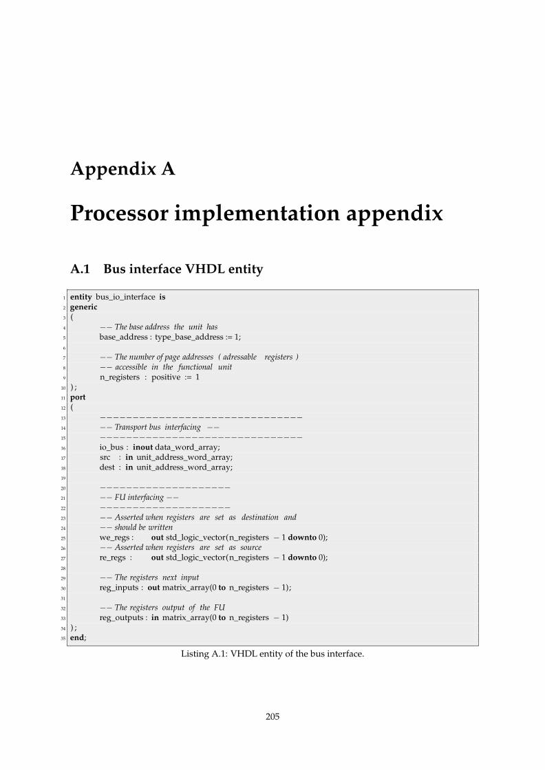
Appendix A

Processor implementation appendix

A.1 Bus interface VHDL entity

1 entity bus_io_interface is2 generic3 (4 −− The base address the unit has5 base_address : type_base_address := 1;6

7 −− The number of page addresses ( adressable registers )8 −− accessible in the functional unit9 n_registers : positive := 1

10 ) ;11 port12 (13 −−−−−−−−−−−−−−−−−−−−−−−−−−−−−−−14 −− Transport bus interfacing −−15 −−−−−−−−−−−−−−−−−−−−−−−−−−−−−−−16 io_bus : inout data_word_array;17 src : in unit_address_word_array;18 dest : in unit_address_word_array;19

20 −−−−−−−−−−−−−−−−−−−−21 −− FU interfacing −−22 −−−−−−−−−−−−−−−−−−−−23 −− Asserted when registers are set as destination and24 −− should be written25 we_regs : out std_logic_vector(n_registers − 1 downto 0);26 −− Asserted when registers are set as source27 re_regs : out std_logic_vector(n_registers − 1 downto 0);28

29 −− The registers next input30 reg_inputs : out matrix_array(0 to n_registers − 1);31

32 −− The registers output of the FU33 reg_outputs : in matrix_array(0 to n_registers − 1)34 ) ;35 end;

Listing A.1: VHDL entity of the bus interface.

205

APPENDIX A. PROCESSOR IMPLEMENTATION APPENDIX

A.2 Functional units memory map

A.2.1 Arithmetic and logic unit

Address RW mode Trigger Name Description

0 RW No A Operand A1 RW Yes B Operand B2 R No ADD A+B3 R No SUB A−B4 R No OR A ∨B5 R No AND A ∧B6 R No NOT ¬B7 R No XOR A⊕B8 R No MULTlow (A ·B)[31...0]

9 R No MULThigh (A ·B)[63...32]

Table A.1: ALU functional unit memory map.

A.2.2 Shift parallel unit

A generic parameter can configure the parallel shift unit to include or not the rotation operation.

Address RW mode Trigger Name Description

0 RW Yes A Operand A1 RW No N Number of bits for the operation2 R No Shift right A� N3 R No Shift right arithmetic (A� N)arith

4 R No Shift left A� N5 R No Rotate left A x B6 R No Rotate right A y A

Table A.2: Parallel shifter memory map.

A.2.3 Concatenation

This unit is automatically used by the assembler to generate long immediates, as described in section3.8.1.

Address RW mode Trigger Name Description

0 W No A Operand A, width = size of short immediate value1 W No B Operand B, width = size of short immediate value0 R No OUT Out = (A� 16) ∨B1 R No ZERO Always zero

Table A.3: Concatenation unit memory map.

A.2.4 Comparison / Condition unit

This unit is mostly used to generate conditions for jumps, as described in section 3.8.2.

206

A.2. FUNCTIONAL UNITS MEMORY MAP

Address RW mode Trigger Name Description

0 RW Yes OP_A Operand A1 RW No OP_B Operand B2 RW No OPCODE Selects the operation performed3 R No RESULT Depending on OPCODE: A < 0, A > 0, A = 0, A 6= 0, A > B,

A ≥ B, A < B, A ≤ B, A = B, A 6= B

Table A.4: Condition functional unit memory map.

A.2.5 GPIO

This unit can be used to provide general-purpose I/O pins to the processor to interface to the outsideworld.

Address RW mode Trigger Name Description

0 RW Yes GPIO_OUT Output word on GPIO pins. The number of GPIO pins foroutput is generic.

1 R No GPIO_IN Value read on GPIO pins. The number of GPIO pins for inputis generic.

Table A.5: GPIO functional unit memory map.

A.2.6 MERCURY unit

This unit is used to interface to the CONFETTI subsystem via the standard MERCURY interface, asdescribed in section 8.4.1.

Address RW mode Trigger Name Description

0 RW Yes STATUS The status register of the unita.1 RW No DMAstart Start address of DMA for MERCURY to memory write.2 RW No DMAend Max address allowed for DMA write.3 W Yes RST Any value written resets the new data flag.3 R No SIZE The size of the last received packet.4 W Yes SEND Pass the written data to the MERCURY sender.4 R No HEADER Header of the last received packet.

a

- ACCEPT_DMA_MASK (bit 0, lsb): 1 if the unit should accept new incoming data, if set to 0 the unit receiver keeps its RDYline deasserted;

- ALLOW_RECONFIG (bit 1): 1 if the unit is allowed to accept new code and reboot, if set to 0 the arrival of a packet with anew code will be ignored;

- WRITE_IN_PROGRESS (bit 2): 1 if MERCURY is currently receiving data;

- NEW_DATA_FLAG (bit 3): 1 if MERCURY receiver has finished writing a whole packet to memory;

- CAN_SEND_DATA (bit 4): 1 if MERCURY sender is ready to handle a new packet of data;

- RECEIVER_EMPTY (bit 5): 1 if there are data in the receiver waiting to be copied with DMA.

Table A.6: Mercury FU memory map.

207

APPENDIX A. PROCESSOR IMPLEMENTATION APPENDIX

A.2.7 Display interface

This unit interfaces with the display area on top of the cell in the CONFETTI platform, as described insection 8.4.2.

Address RW mode Trigger Name Description

0 R No X X-coordinate of this CPU in the CONFETTI grid.1 R No Y Y-coordinate of this CPU in the CONFETTI grid.0 W No ADDR Address of the pixel to modify.1 W Yes COLOR Sets the color of the pixel.2 R No TOUCH # of seconds the touch sensor has been pressed continuously.3 R No GRAPHIC Last pixel value written to the graphic memory.

[4. . . 7] RW No GR[0. . . 3] General purpose register [0. . . 3].

Table A.7: Display FU memory map.

A.2.8 Timer

This unit can be used to accurately measure time with a µs resolution. The unit uses a generic defini-tion of the processor speed, provided in the entity of the unit, to accomodate different clock periods.More precisely, the counter is updated every ( clk_frequency

106 − 1).

Address RW mode Trigger Name Description

0 R No US_COUNTER Number of µs since last processor or timer reset.0 W Yes RST Resets the timer counter.

Table A.8: Timer FU memory map.

A.2.9 SRAM interface

This functional unit can be used to connect asynchronous SRAM memory to ULYSSE, as described insection 3.7.2.

Address RW mode Trigger Name – Function Description

0 RW No SP1 Stack pointer number 11 RW No SP2 Stack pointer number 22 RW No DATA Memory data register3 W Yes Load absolute Data←Memory(Address)4 W Yes Store absolute Memory(Address)← Data5 W Yes Load with offset 1 Data←Mem(Address + SP1)6 W Yes Load with offset 2 Data←Mem(Address + SP2)7 W Yes Store with offset 1 Mem(Address + SP1)← Data8 W Yes Store with offset 2 Mem(Address + SP2)← Data

Table A.9: SRAM FU Interface memory map.

A.2.10 Assertion unit

This unit is used in the context of asserted simulation (see section 5.2).

208

A.2. FUNCTIONAL UNITS MEMORY MAP

Address RW mode Trigger Name – Function Description

0 W No A Operand A1 W No B Operand B2 W No LINE Line of code currently asserted (to be displayed in

MODELSIMTM in case of error).3 W Yes STOP Stop simulation in MODELSIMTM at current line.4 W Yes DUMPstart Start dumping memory in MODELSIMTM with address

DUMPstart.5 W Yes DUMPaddress Display memory content of address DUMPaddress in

MODELSIMTM.6 W Yes DUMPstop Stop dumping memory in MODELSIMTM.

Table A.10: Assertion FU memory map.

A.2.11 Divider unit

This unit is articulated around an IP module published by Xilinx and accessible with its CoreGen tool.As this divider is pipelined, maximum throughput is achieved when data are input every cycle anddivisions made in a row, especially since initial latency in the chosen configuration1 is 41 cycles. As themodule does not provide a signal to indicate valid results, we had to implement a state machine thatcounts the number of cycle corresponding to latency to know when the operator completes, assertingthe busy bit of the unit that time.

Address RW mode Trigger Name Description

0 RW No OP_A Dividend1 RW Yes OP_B Divisor2 R No QUOTIENT Dividend/Divisor, with “/” integer division3 R No REMAINDER Dividend−Quotient ·Divisor

Table A.11: Divider unit memory map.

1Dividend, divisor, remainder and quotient all on 32 bits

209

APPENDIX A. PROCESSOR IMPLEMENTATION APPENDIX

A.3 Functional unit code samples

A.3.1 Concatenation unit

1 −−2 −− EPFL3 −− Ulysse processor − Concatenation unit for 16 bits immediate values4 −− Pierre−Andre Mudry, 20085 −−6

7 library ieee , ulysse;8 USE ieee.numeric_std.ALL;9 USE ieee.std_logic_1164.ALL;

10 use ieee .std_logic_unsigned.all;11 use ulysse. ulysse_utils . all ;12

13 architecture str of concat is14 signal reg_0_in, reg_0_out, reg_1_in, reg_1_out : type_immediate;15 signal big_reg_0_in, big_reg_1_in : data_word;16

17 subtype data_range is integer range immediate_size − 1 downto 0;18 signal reg_out : data_word;19 signal we_regs : std_logic_vector(1 downto 0);20 signal we_0, we_1 : std_logic ;21 begin22

23 −− Asserted when writing to page 024 we_0 <= we_regs(0);25 −− Asserted when writing to page 126 we_1 <= we_regs(1);27

28 −− Size mapping29 reg_0_in <= big_reg_0_in(data_range);30 reg_1_in <= big_reg_1_in(data_range);31

32 −− This FU is never busy, latency 133 busy <= ’0’;34

35 −− Register to store the low immediate value36 i_reg_0 : entity ulysse.reg generic map (register_width => immediate_size)37 port map (clk => clk, we => we_0, rst => rst , input => reg_0_in,38 output => reg_0_out);39

40 −− Register to store the high immediate value41 i_reg_1 : entity ulysse.reg generic map (register_width => immediate_size)42 port map (clk => clk, we => we_1, rst => rst , input => reg_1_in,43 output => reg_1_out);44

45 −− Instantiate the bus interface46 i_bus_in : entity ulysse.bus_io_interface generic map47 (base_address => base_address, n_registers => 2) port map48 (io_bus => io_bus,49 src => src,50 dest => dest,51 we_regs => we_regs,52 re_regs => open,53 reg_inputs(0) => big_reg_0_in,54 reg_inputs(1) => big_reg_1_in,

210

A.3. FUNCTIONAL UNIT CODE SAMPLES

55 reg_outputs(0) => reg_out,56 reg_outputs(1) => zero_dw −− Always zero57 ) ;58

59 −− Concatenate the two immediate values60 process(reg_1_out, reg_0_out)61 begin62 reg_out <= reg_1_out & reg_0_out;63 end process;64

65 end str ;

Listing A.2: Concatenation unit implementation.

211

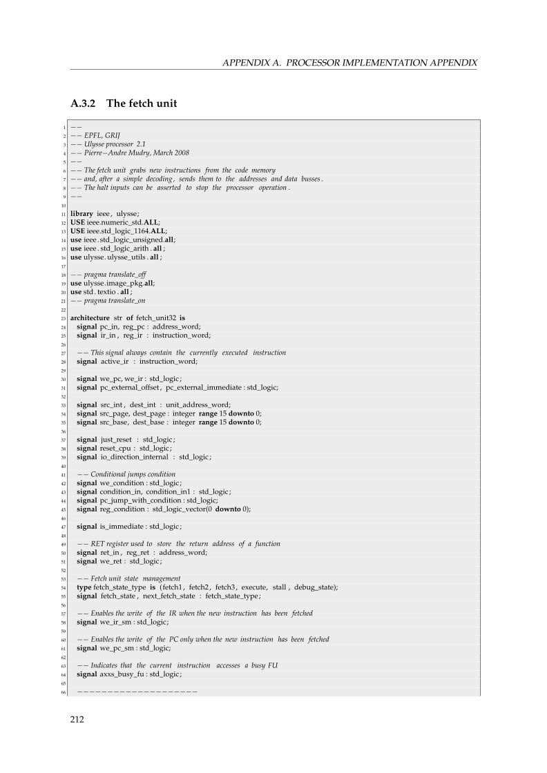
APPENDIX A. PROCESSOR IMPLEMENTATION APPENDIX

A.3.2 The fetch unit

1 −−2 −− EPFL, GRIJ3 −− Ulysse processor 2.14 −− Pierre−Andre Mudry, March 20085 −−6 −− The fetch unit grabs new instructions from the code memory7 −− and, after a simple decoding , sends them to the addresses and data busses .8 −− The halt inputs can be asserted to stop the processor operation .9 −−

10

11 library ieee , ulysse;12 USE ieee.numeric_std.ALL;13 USE ieee.std_logic_1164.ALL;14 use ieee .std_logic_unsigned.all;15 use ieee . std_logic_arith . all ;16 use ulysse. ulysse_utils . all ;17

18 −− pragma translate_off19 use ulysse.image_pkg.all;20 use std. textio . all ;21 −− pragma translate_on22

23 architecture str of fetch_unit32 is24 signal pc_in, reg_pc : address_word;25 signal ir_in , reg_ir : instruction_word;26

27 −− This signal always contain the currently executed instruction28 signal active_ir : instruction_word;29

30 signal we_pc, we_ir : std_logic ;31 signal pc_external_offset , pc_external_immediate : std_logic;32

33 signal src_int , dest_int : unit_address_word;34 signal src_page, dest_page : integer range 15 downto 0;35 signal src_base, dest_base : integer range 15 downto 0;36

37 signal just_reset : std_logic ;38 signal reset_cpu : std_logic ;39 signal io_direction_internal : std_logic ;40

41 −− Conditional jumps condition42 signal we_condition : std_logic ;43 signal condition_in, condition_in1 : std_logic ;44 signal pc_jump_with_condition : std_logic;45 signal reg_condition : std_logic_vector(0 downto 0);46

47 signal is_immediate : std_logic ;48

49 −− RET register used to store the return address of a function50 signal ret_in , reg_ret : address_word;51 signal we_ret : std_logic ;52

53 −− Fetch unit state management54 type fetch_state_type is (fetch1 , fetch2 , fetch3 , execute, stall , debug_state);55 signal fetch_state , next_fetch_state : fetch_state_type;56

57 −− Enables the write of the IR when the new instruction has been fetched58 signal we_ir_sm : std_logic;59

60 −− Enables the write of the PC only when the new instruction has been fetched61 signal we_pc_sm : std_logic;62

63 −− Indicates that the current instruction accesses a busy FU64 signal axxs_busy_fu : std_logic ;65

66 −−−−−−−−−−−−−−−−−−−−

212

A.3. FUNCTIONAL UNIT CODE SAMPLES

67 −− Debugging related68 −−−−−−−−−−−−−−−−−−−−69 −− pragma translate_off70 −− Stores the instruction strings for debugging purposes71 type array_instr is array (integer range <>) of string(1 to 60) ;72 signal currentInstr : string(1 to 60) ;73

74 −− Reads the file containing the instructions in a textual form so they75 −− can be displayed directly in the simulator76 procedure readIstrFile( instr : inout array_instr) is77 file data_file : text open read_mode is debug_istr_fileName;78 variable l : line ;79 variable current_address : natural := 0;80 variable s : string(1 to 60) ;81 begin82 While Not Endfile(data_file) Loop83 s := (others => ’ ’) ;84 Readline(data_file , l ) ;85 Read(l, s( l ’range)); −− Reads the string from the line86 instr (current_address) := s ;87 current_address := current_address + 1;88 End Loop;89 end procedure readIstrFile;90 −− pragma translate_on91

92 begin93

94 reset_cpu <= restart_cpu or rst ;95

96 −−−−−−−−−−−−−−−−−−−−−−−−−−−−−−−−−−−−−−−−−97 −− Registers present in the fetch unit98 −−−−−−−−−−−−−−−−−−−−−−−−−−−−−−−−−−−−−−−−−99 i_pc : entity ulysse.reg generic map (register_width => (memory_height))

100 port map (clk => clk, we => we_pc, rst => reset_cpu, input => pc_in, output => reg_pc);101

102 i_ir : entity ulysse.reg generic map (register_width => instruction_width∗instruction_slots)103 port map (clk => clk, rst => reset_cpu, we => we_ir, input => ir_in, output => reg_ir) ;104

105 i_condition : entity ulysse. regbit106 port map (clk => clk, rst => reset_cpu, we => we_condition, input => condition_in, output => reg_condition(0));107

108 i_jrst : entity ulysse. regbit109 port map (clk => clk, rst => ’0’, we => ’1’, input => rst , output => just_reset ) ;110

111 i_ret : entity ulysse.reg generic map(register_width => memory_height)112 port map (clk => clk, rst => reset_cpu, we => we_ret, input => ret_in, output => reg_ret);113

114 assert (current_n_fu = 4 or current_n_fu = 8 or current_n_fu = 16 or current_n_fu = 32 or current_n_fu = 64)115 report string ’("Number of FU specified not a power of 2 or not < 128") severity failure;116

117

118 −− Halt and write signals must be able to reflect the busy conditions coming from the119 −− functional units120 we_ir <= (not halt ) and we_ir_sm;−−and not(axxs_busy_fu);121

122 −− The IR is the content of the memory location pointed by the PC123 ir_in <= mem_q;124

125 −−−−−126 −− BUSY FU Management127 −− The idea here is when an operation takes more than one cycle it asserts128 −− it’s busy flag and, while no other operation tries to read or write to129 −− the busy FU, the processor behaves normally. However, if an operation130 −− needs to read or write the busy FU, the processor is halted until131 −− the FU is no more busy in order to resolve the dependency automatically .132 −−−−−133 −− Is the currently active instruction containing an immediate value ?134 process(active_ir )

213

APPENDIX A. PROCESSOR IMPLEMENTATION APPENDIX

135 begin136 is_immediate <= ’0’;137 if ( active_ir (is_immediate_field) = ’1’) then138 is_immediate <= ’1’;139 end if ;140 end process;141

142 −− SRC and DST page and base extraction143 process(src_int , dest_int)144 begin145 src_page <= extract_page(src_int) ;146 dest_page <= extract_page(dest_int);147

148 src_base <= to_integer(ieee .numeric_std.unsigned(src_int(7 downto 4)));149 dest_base <= to_integer(ieee .numeric_std.unsigned(dest_int(7 downto 4)));150 end process;151

152 −− IO Process for transport bus 1153 process(active_ir , reg_pc, is_immediate, io_bus, halt ,154 reg_ret , fetch_state , reg_ir , src_base, src_page,155 dest_base, dest_page)156 begin157 io_bus(0) <= z_dw;158

159 pc_external_offset <= ’0’;160 pc_external_immediate <= ’0’;161 pc_jump_with_condition <= ’0’;162 condition_in1 <= ’0’;163

164 −− RET165 we_ret <= ’0’;166 ret_in <= (others => ’0’) ;167

168 −− Default is to read the io_bus169 io_direction_internal <= ’1’;170

171 −− If the fetch unit is used as a source172 if (src_base = base_address and fetch_state = execute) then173 io_direction_internal <= ’0’;174

175 −− Output to bus the immediate value contained in the instruction176 if (is_immediate = ’1’) then177 io_bus(0) <= sxt( active_ir (immediate_field), data_width);178 else179 −− Output to the bus the PC or the IR180 case(src_page) is181 when 1 => io_bus(0) <= pad_with_zeroes(reg_pc, data_width);182 when 2 => io_bus(0) <= pad_with_zeroes(reg_ir, data_width);183 when 3 => io_bus(0) <= pad_with_zeroes(reg_ret, data_width);184 −−when 4 => io_bus(0) <= ext(processor_id , data_width) ;185 when others => null;186 end case;187 end if ;188 end if ;189

190 −− PC modifications from the outside ( relative and absolute jumps)191 −− Aka the fetch unit is used as a destination192 if (dest_base = base_address and halt = ’0’) then193 −− Input from bus194 case(dest_page) is195 when 1 =>196 pc_external_offset <= ’1’;197 when 2 =>198 pc_external_immediate <= ’1’;199 when 3 =>200 ret_in <= io_bus(0)(memory_height − 1 downto 0);201 we_ret <= ’1’;202 when 4 =>

214

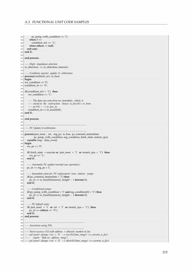
A.3. FUNCTIONAL UNIT CODE SAMPLES

203 pc_jump_with_condition <= ’1’;204 when 5 =>205 condition_in1 <= ’1’;206 when others => null;207 end case;208 end if ;209

210 end process;211

212 −− High−impedance selection213 io_direction <= io_direction_internal ;214

215 −− Condition register update & arbitration216 process(condition_in1, io_bus)217 begin218 we_condition <= ’0’;219 condition_in <= ’0’;220

221 if (condition_in1 = ’1’) then222 we_condition <= ’1’;223

224 −− The data can come from an immediate, which is225 −− stored in the instruction (hence io_bus (0) ) or from226 −− an FU −−> io_bus_in227 condition_in <= io_bus(0)(0) ;228 end if ;229

230 end process;231

232 −−−−−−−−−−−−−−−−−−−−−−−−−−−−−233 −− PC Update & arbitration234 −−−−−−−−−−−−−−−−−−−−−−−−−−−−−235 process( just_reset , rst , reg_pc, io_bus, pc_external_immediate,236 pc_jump_with_condition, reg_condition, fetch_state, restart_cpu)237 variable tmp : data_word;238 begin239 we_pc <= ’0’;240

241 if ( fetch_state = execute or just_reset = ’1’ or restart_cpu = ’1’) then242 we_pc <= ’1’;243 end if ;244

245 −− Automatic PC update (normal case operation )246 pc_in <= reg_pc + 1;247

248 −− Immediate value for PC replacement (non relative jump)249 if (pc_external_immediate = ’1’) then250 pc_in <= io_bus(0)(memory_height − 1 downto 0);251 end if ;252

253 −− Conditional jumps254 if (pc_jump_with_condition = ’1’ and reg_condition(0) = ’1’) then255 pc_in <= io_bus(0)(memory_height − 1 downto 0);256 end if ;257

258 −− PC default value259 if ( just_reset = ’1’ or rst = ’1’ or restart_cpu = ’1’) then260 pc_in <= (others => ’0’) ;261 end if ;262 end process;263

264 −−−−−−−−−−−−−−−−−−−−−−−−−−−−265 −− Assertions using PSL266 −−−−−−−−−−−−−−−−−−−−−−−−−−−−267 −− Never access a FU with address > allowed number of fus268 −− psl assert always ( rst = ’0’ −> (src(0) (base_range) <= current_n_fu))269 −− report "Bad src address range";270 −− psl assert always ( rst = ’0’ −> (dest(0) (base_range) <= current_n_fu))

215

APPENDIX A. PROCESSOR IMPLEMENTATION APPENDIX

271 −− report "Bad dest address range";272 process(src_int , dest_int , fetch_state )273 begin274 if ( fetch_state = execute) then275 src (0) <= pad_with_zeroes(src_int(7 downto 0), 15);276 dest(0) <= pad_with_zeroes(dest_int(7 downto 0), 15);277 else278 src (0) <= (others => ’0’) ;279 dest(0) <= (others => ’0’) ;280 end if ;281 end process;282

283 −− Code memory interface284 process(reg_pc)285 begin286 mem_address <= reg_pc;287 end process;288

289 process(fetch_state , ir_in , reg_ir)290 begin291 if ( fetch_state = execute) then292 active_ir <= ir_in ;293 else294 active_ir <= reg_ir;295 end if ;296 end process;297

298 −−−−−−−−−−−−−−−−−−−−−−−−−−−−299 −− Fetch unit state machine300 −−−−−−−−−−−−−−−−−−−−−−−−−−−−301 fetch_sm :302 process(fetch_state , busy_flags, is_immediate, active_ir , dest_base, src_base, halt )303 begin304 mem_req <= ’0’;305 we_ir_sm <= ’0’;306 we_pc_sm <= ’0’;307 axxs_busy_fu <= ’0’;308

309 src_int <= (others => ’0’) ;310 dest_int <= (others => ’0’) ;311

312 case fetch_state is313 when fetch1 =>314 debug_out <= x"1";315

316 if (halt = ’1’) then317 next_fetch_state <= debug_state;318 else319 we_pc_sm <= ’1’;320 next_fetch_state <= fetch2;321 mem_req <= ’1’;322 end if ;323

324 when fetch2 =>325 debug_out <= x"2";326 mem_req <= ’1’;327 next_fetch_state <= fetch3;328

329 when fetch3 =>330 debug_out <= x"3";331 mem_req <= ’1’;332 next_fetch_state <= execute;333

334 when execute =>335 debug_out <= x"4";336 we_ir_sm <= ’1’;337

338 −− Normal case

216

A.3. FUNCTIONAL UNIT CODE SAMPLES

339 next_fetch_state <= fetch1;340 mem_req <= ’1’; −− Indicate memory that next state should be loading341

342 −− Internal source and destination busses assignment343 dest_int <= active_ir ( destination_field ) ;344 if (is_immediate = ’0’) then345 src_int <= active_ir (source_field) ;346 end if ;347

348 −− If the destination we want is busy,349 −− then stall until free again350 if (busy_flags(dest_base) = ’1’) then351 next_fetch_state <= stall ;352 axxs_busy_fu <= ’1’;353 mem_req <= ’0’;354 elsif (is_immediate = ’0’ and busy_flags(src_base) = ’1’) then355 −− If the source we want is busy (and not an immediate) ,356 −− then stall until free again357 axxs_busy_fu <= ’1’;358 next_fetch_state <= stall ;359 mem_req <= ’0’;360 end if ;361

362 when stall =>363 debug_out <= x"5";364 dest_int <= active_ir ( destination_field ) ;365

366 if (is_immediate = ’0’) then367 src_int <= active_ir (source_field) ;368 end if ;369

370 −− If the destination we want is busy,371 −− then stall until free again372 if (busy_flags(dest_base) = ’1’) then373 next_fetch_state <= stall ;374 axxs_busy_fu <= ’1’;375 elsif (is_immediate = ’0’ and busy_flags(src_base) = ’1’) then376 −− If the source we want is busy (and not an immediate) ,377 −− then stall until free again378 next_fetch_state <= stall ;379 axxs_busy_fu <= ’1’;380 else381 next_fetch_state <= fetch1;382 mem_req <= ’1’; −− Indicate memory that next state should be loading383 end if ;384

385 when debug_state =>386 debug_out <= x"6";387 next_fetch_state <= debug_state;388

389 if (halt = ’0’) then390 next_fetch_state <= fetch1;391 mem_req <= ’1’; −− Indicate memory that next state should be loading392 end if ;393

394 end case;395 end process;396

397 −− Fetch unit State machine updater398 fetch_state_updater:399 process(clk, rst )400 begin401 if ( rst = ’1’) then402 fetch_state <= fetch1;403 elsif (rising_edge(clk)) then404 fetch_state <= next_fetch_state;405 end if ;406 end process;

217

APPENDIX A. PROCESSOR IMPLEMENTATION APPENDIX

407

408 −−−−−−−−−−−−−−−−−−−−−−−−−−−−409 −− The rest of this file is used only during debugging to help410 −− the programmer.411 −−−−−−−−−−−−−−−−−−−−−−−−−−−−412 −− pragma translate_off413 process(reg_pc, fetch_state , pc_in)414 variable instructions : array_instr(0 to 262143);415 variable initDone : boolean := false ;416 begin417 −− At first call , load the file containing the textual418 −− representation of the instructions and put it in the419 −− instructions array420 if (not initDone) then421 readIstrFile ( instructions ) ;422 currentInstr <= instructions (0) ;423 initDone := true;424 else425 if ( fetch_state = execute) then426 currentInstr <= instructions(to_integer(ieee .numeric_std.unsigned(pc_in)));427 else428 currentInstr <= instructions(to_integer(ieee .numeric_std.unsigned(reg_pc)));429 end if ;430 end if ;431 end process;432

433 −− Dumps various debugging information such as434 −− number of cycles, current instruction ... in the simulator435 process(clk)436 variable d : line ;437 variable clk_cycle : integer := 0;438 variable clk_cycle_since_rst : integer := 0;439 variable cycle_count : integer := 0;440 begin441 if (rising_edge(clk)) then442 if ( rst = ’0’) then443 clk_cycle := clk_cycle + 1;444 clk_cycle_since_rst := clk_cycle_since_rst + 1;445

446 if (dump_instr and next_fetch_state = execute) then447 cycle_count := cycle_count + 1;448 write(d, string ’("* Clk since begin " & integer’image(clk_cycle) & " / Total clk " & integer’image(

clk_cycle_since_rst) & " - cycle " & integer’image(cycle_count)));449 writeline(output, d);450 write(d, string ’(" * Execute " & currentInstr));451 writeline(output, d);452 end if ;453

454 if (dump_instr = false and next_fetch_state = execute) then455 if ( clk_cycle_since_rst mod 1000 = 0) then456 write(d, string ’("+"));457 writeline(output, d);458 end if ;459 end if ;460 else461 clk_cycle_since_rst := 0;462 cycle_count := 0;463 end if ;464 end if ;465 end process;466 −− pragma translate_on467 end str ;

Listing A.3: Fetch unit code.

218

A.3. FUNCTIONAL UNIT CODE SAMPLES

A.3.3 The memory unit

1 library ieee , ulysse;2 use ieee .numeric_std.all;3 use ieee .std_logic_1164.all ;4 use ieee . std_logic_arith . all ;5 use ieee .std_logic_unsigned.all;6 use ulysse. ulysse_utils . all ;7

8 −− pragma translate_off9 use ulysse.image_pkg.all;

10 use std. textio . all ;11 −− pragma translate_on12

13 entity harvard_memory_unit is14 generic15 (16 base_address : type_base_address := 1217 ) ;18 port19 (20 clk : in std_logic ;21 clk4x : in std_logic ;22 rst : in std_logic ;23 is_idle : out std_logic ;24

25 −− Ulysse standard access26 busy : out std_logic ;27 io_bus : inout data_word_array;28 src : in unit_address_word_array;29 dest : in unit_address_word_array;30

31 −− Connexion to fetch unit32 fetch_mem_address : in address_word;33 fetch_mem_data : out instruction_word;34 fetch_mem_req : in std_logic;35

36 −− External control of memory37 external_req : in std_logic ;38 external_address : in address_word;39 external_data : in instruction_word;40 external_rw : in std_logic ; −− Direction of transfer41

42 −− To the SRAMs IO Ports43 a : out address_word;44 d : inout std_logic_vector(half_instruction_width − 1 downto 0);45 nCS0 : out std_logic ;46 nCS1 : out std_logic ;47 nWE : out std_logic;48 nOE : out std_logic ;49 nLB : out std_logic ;50 nUB : out std_logic51 ) ;52 end;53

54 architecture str of harvard_memory_unit is55 signal enable, wr : std_logic ;56

57 signal data_towrite, data_read : data_word;58 signal address : address_word;59

60 type state_type is ( idle , fetch1 , fetch2 , fetch3 , load1, load2, load3, store_operation, prestore_operation);61 signal state , next_state : state_type;62

63 signal we_sp1, we_sp2, we_data : std_logic;64 signal re_sp1, re_sp2, re_data : std_logic ;65 signal sp1_in, reg_sp1 : address_word;66 signal sp2_in, reg_sp2 : address_word;

219

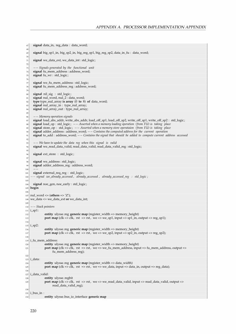
APPENDIX A. PROCESSOR IMPLEMENTATION APPENDIX

67 signal data_in, reg_data : data_word;68

69 signal big_sp1_in, big_sp2_in, big_reg_sp1, big_reg_sp2, data_in_fu : data_word;70

71 signal we_data_ext, we_data_int : std_logic;72

73 −− Signals generated by the functional unit74 signal fu_mem_address : address_word;75 signal fu_wr : std_logic ;76

77 signal we_fu_mem_address : std_logic;78 signal fu_mem_address_reg : address_word;79

80 signal nil_sig : std_logic ;81 signal nul_word, nul_2 : data_word;82 type type_nul_array is array (0 to 8) of data_word;83 signal nul_array_in : type_nul_array;84 signal nul_array_out : type_nul_array;85

86 −− Memory operation signals87 signal load_abs_addr, write_abs_addr, load_off_sp1, load_off_sp2, write_off_sp1, write_off_sp2 : std_logic ;88 signal load_op : std_logic ; −− Asserted when a memory loading operation (from FU) is taking place89 signal store_op : std_logic ; −− Asserted when a memory store operataion (from FU) is taking place90 signal adder_address : address_word; −− Contains the computed address for the current operation91 signal to_add : address_word; −− Contains the signal that should be added to compute current address accessed92

93 −− We have to update the data reg when this signal is valid94 signal we_read_data_valid, read_data_valid, read_data_valid_reg : std_logic;95

96 signal ext_store : std_logic ;97

98 signal we_address : std_logic;99 signal adder_address_reg : address_word;

100 −−101 signal external_req_reg : std_logic ;102 −− signal we_already_accessed , already_accessed , already_accessed_reg : std_logic ;103

104 signal noe_gen, noe_early : std_logic ;105 begin106

107 nul_word <= (others => ’Z’);108 we_data <= we_data_ext or we_data_int;109

110 −− Stack pointers111 i_sp1:112 entity ulysse.reg generic map (register_width => memory_height)113 port map (clk => clk, rst => rst , we => we_sp1, input => sp1_in, output => reg_sp1);114

115 i_sp2:116 entity ulysse.reg generic map (register_width => memory_height)117 port map (clk => clk, rst => rst , we => we_sp2, input => sp2_in, output => reg_sp2);118

119 i_fu_mem_address:120 entity ulysse.reg generic map (register_width => memory_height)121 port map (clk => clk, rst => rst , we => we_fu_mem_address, input => fu_mem_address, output =>

fu_mem_address_reg);122

123 i_data:124 entity ulysse.reg generic map (register_width => data_width)125 port map (clk => clk, rst => rst , we => we_data, input => data_in, output => reg_data);126

127 i_data_valid:128 entity ulysse. regbit129 port map (clk => clk, rst => rst , we => we_read_data_valid, input => read_data_valid, output =>

read_data_valid_reg);130

131 i_bus_in :132 entity ulysse.bus_io_interface generic map

220

A.3. FUNCTIONAL UNIT CODE SAMPLES

133 (base_address => base_address, n_registers => 9) port map134 (io_bus => io_bus,135 src => src,136 dest => dest,137 we_regs(0) => we_sp1, −− sp1 = io_bus138 we_regs(1) => we_sp2, −− sp2 = io_bus139 we_regs(2) => we_data_ext,−− data = io_bus140 we_regs(3) => load_abs_addr, −− data = mem(abs)141 we_regs(4) => write_abs_addr, −− mem(abs) = data142 we_regs(5) => load_off_sp1, −− data = mem(SP1 + offset1)143 we_regs(6) => load_off_sp2, −− data = mem(SP2 + offset2)144 we_regs(7) => write_off_sp1, −− mem(SP1 + offset1) = data145 we_regs(8) => write_off_sp2, −− mem(SP2 + offset2) = data146

147 re_regs(0) => re_sp1, −− io_bus = sp1148 re_regs(1) => re_sp2, −− io_bus = sp2149 re_regs(2) => re_data, −− io_bus = data150 re_regs(3) => nil_sig ,151 re_regs(4) => nil_sig ,152 re_regs(5) => nil_sig ,153 re_regs(6) => nil_sig ,154 re_regs(7) => nil_sig ,155 re_regs(8) => nil_sig ,156

157 reg_inputs(0) => big_sp1_in,158 reg_inputs(1) => big_sp2_in,159 reg_inputs(2) => data_in_fu,160 reg_inputs(3) => nul_array_in(3),161 reg_inputs(4) => nul_array_in(4),162 reg_inputs(5) => nul_array_in(5),163 reg_inputs(6) => nul_array_in(6),164 reg_inputs(7) => nul_array_in(7),165 reg_inputs(8) => nul_array_in(8),166

167 reg_outputs(0) => big_reg_sp1,168 reg_outputs(1) => big_reg_sp2,169 reg_outputs(2) => reg_data,170 reg_outputs(3) => nul_array_out(3),171 reg_outputs(4) => nul_array_out(4),172 reg_outputs(5) => nul_array_out(5),173 reg_outputs(6) => nul_array_out(6),174 reg_outputs(7) => nul_array_out(7),175 reg_outputs(8) => nul_array_out(8)176 ) ;177

178 sp1_in <= big_sp1_in(memory_height − 1 downto 0);179 sp2_in <= big_sp2_in(memory_height − 1 downto 0);180 big_reg_sp1 <= ext(reg_sp1, data_width);181 big_reg_sp2 <= ext(reg_sp2, data_width);182

183 −− Asserted when a FU loading operation is taking place184 load_op <= load_off_sp1 or load_off_sp2 or load_abs_addr;185 store_op <= write_abs_addr or write_off_sp1 or write_off_sp2;186

187 sram_controller :188 entity ulysse.sram_controller(str) port map189 (190 clk => clk,191 clk4x => clk4x,192 rst => rst ,193 −− Ctrl signals194 enable => enable,195 address => address,196 data_towrite => data_towrite,197 data_read => data_read,198 wr => wr,199 −− SRAM IO pins200 nCS0_reg => nCS0,

221

APPENDIX A. PROCESSOR IMPLEMENTATION APPENDIX

201 nCS1_reg => nCS1,202 a => a,203 d => d,204 nWE => nWE,205 nOE => nOE_gen,206 nLB => nLB,207 nUB => nUB208 ) ;209

210 datasrc_chooser:211 process(external_req, external_data, we_data_int, data_read, data_in_fu)212 begin213 if (external_req = ’1’) then214 data_in <= external_data;215 elsif (we_data_int = ’1’) then216 data_in <= data_read;217 else218 data_in <= data_in_fu;219 end if ;220 end process;221

222 −−−−−−−−−−−−−−−−−−−−−−−−−−−223 −− Assertions using PSL224 −−−−−−−−−−−−−−−−−−−−−−−−−−−225

226 −− Make sure that the address won’t change when fetching a new data227 −−−− psl assert always (( rst = ’0’ and fetch_mem_req = ’1’) −> next(prev(fetch_mem_address) = fetch_mem_address))@(

rising_edge( clk ) )228 −−−− report "Address not stable ";229

230 nOE <= noe_gen or noe_early;231

232 process(state , fetch_mem_req, fetch_mem_address,233 data_read, read_data_valid_reg,234 load_op, store_op, external_req,235 reg_data, adder_address_reg)236 begin237 −− Memory ctrl238 enable <= ’0’;239 address <= (others => ’0’) ;240 wr <= ’0’;241 data_towrite <= reg_data;242

243 −− Data register input244 we_data_int <= ’0’;245

246 −− Ctrl for the various FU operations247 fu_mem_address <= (others => ’0’);248 fu_wr <= ’0’;249 we_fu_mem_address <= ’0’;250

251 we_address <= ’0’;252

253 busy <= ’0’;254

255 we_read_data_valid <= ’0’;256 read_data_valid <= ’0’;257 fetch_mem_data <= data_read;258

259 ext_store <= ’0’;260 is_idle <= ’0’;261

262 noe_early <= ’0’;263

264 case state is265 when idle =>266 next_state <= idle ;267 is_idle <= ’1’;

222

A.3. FUNCTIONAL UNIT CODE SAMPLES

268

269 −− Register the data read if previous operation was a read270 if (read_data_valid_reg = ’1’) then271 assert not(is_x(data_read)) report272 string ’("Data read not valid. Memory not initialized before read ?")273 severity failure ;274 we_read_data_valid <= ’1’;275 read_data_valid <= ’0’;276 we_data_int <= ’1’; −− Data is now valid277 is_idle <= ’0’;278 end if ;279

280 −− If memory is controlled from the outside of the CPU281 −− let’s be controlled from the outside282 if (external_req = ’1’) then283 −− Write current data284 we_data_int <= ’1’;285 next_state <= prestore_operation;286 we_address <= ’1’;287 ext_store <= ’1’;288 else289 −− Fetch unit requests access to the RAM290 if (fetch_mem_req = ’1’) then291 next_state <= fetch1;292 end if ;293

294 −− Excecute phase requests a load295 if (load_op = ’1’) then296 next_state <= load1;297 we_address <= ’1’;298 busy <= ’1’;299 end if ;300

301 −− Execute phase request a write302 if (store_op = ’1’) then303 next_state <= prestore_operation;304 we_address <= ’1’;305 busy <= ’1’;306 end if ;307 end if ;308

309 when fetch1 =>310 −− Register the data read if previous operation was a read311 if (read_data_valid_reg = ’1’) then312 assert not(is_x(data_read)) report313 string ’("Data read not valid. Memory not initialized before read ?")314 severity failure ;315 we_read_data_valid <= ’1’;316 read_data_valid <= ’0’;317 we_data_int <= ’1’; −− Data is now valid318 end if ;319

320 noe_early <= ’0’;321 wr <= ’0’;322 enable <= ’1’;323 address <= fetch_mem_address;324 next_state <= fetch2;325

326 −− When the fetch unit has the control327 when fetch2 =>328 noe_early <= ’0’;329 address <= fetch_mem_address;330 next_state <= fetch3;331

332 −− When the fetch unit has the control333 when fetch3 =>334 noe_early <= ’0’;335 address <= fetch_mem_address;

223

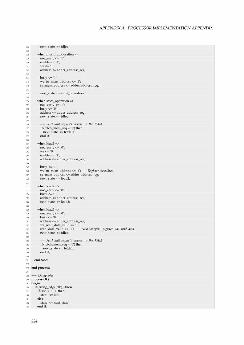
APPENDIX A. PROCESSOR IMPLEMENTATION APPENDIX

336 next_state <= idle ;337

338 when prestore_operation =>339 noe_early <= ’1’;340 enable <= ’1’;341 wr <= ’1’;342 address <= adder_address_reg;343

344 busy <= ’1’;345 we_fu_mem_address <= ’1’;346 fu_mem_address <= adder_address_reg;347

348 next_state <= store_operation;349

350 when store_operation =>351 noe_early <= ’1’;352 busy <= ’0’;353 address <= adder_address_reg;354 next_state <= idle ;355

356 −− Fetch unit requests access to the RAM357 if (fetch_mem_req = ’1’) then358 next_state <= fetch1;359 end if ;360

361 when load1 =>362 noe_early <= ’0’;363 wr <= ’0’;364 enable <= ’1’;365 address <= adder_address_reg;366

367 busy <= ’1’;368 we_fu_mem_address <= ’1’; −− Register the address369 fu_mem_address <= adder_address_reg;370 next_state <= load2;371

372 when load2 =>373 noe_early <= ’0’;374 busy <= ’1’;375 address <= adder_address_reg;376 next_state <= load3;377

378 when load3 =>379 noe_early <= ’0’;380 busy <= ’0’;381 address <= adder_address_reg;382 we_read_data_valid <= ’1’;383 read_data_valid <= ’1’; −− Next clk cycle register the read data384 next_state <= idle ;385

386 −− Fetch unit requests access to the RAM387 if (fetch_mem_req = ’1’) then388 next_state <= fetch1;389 end if ;390

391 end case;392

393 end process;394

395 −− SM updater396 process(clk)397 begin398 if (rising_edge(clk)) then399 if ( rst = ’1’) then400 state <= idle ;401 else402 state <= next_state;403 end if ;

224

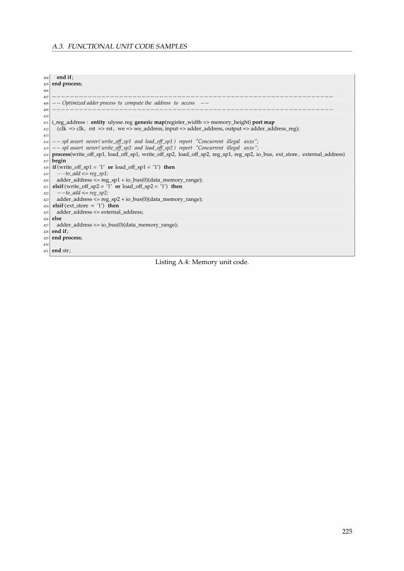
A.3. FUNCTIONAL UNIT CODE SAMPLES

404 end if ;405 end process;406

407 −−−−−−−−−−−−−−−−−−−−−−−−−−−−−−−−−−−−−−−−−−−−−−−−−−−−−−−−−−−−−−−408 −− Optimized adder process to compute the address to access −−409 −−−−−−−−−−−−−−−−−−−−−−−−−−−−−−−−−−−−−−−−−−−−−−−−−−−−−−−−−−−−−−−410

411 i_reg_address : entity ulysse.reg generic map(register_width => memory_height) port map412 (clk => clk, rst => rst , we => we_address, input => adder_address, output => adder_address_reg);413

414 −− spl assert never( write_off_sp1 and load_off_sp1 ) report "Concurrent illegal axxs";415 −− spl assert never( write_off_sp2 and load_off_sp2 ) report "Concurrent illegal axxs";416 process(write_off_sp1, load_off_sp1, write_off_sp2, load_off_sp2, reg_sp1, reg_sp2, io_bus, ext_store , external_address)417 begin418 if (write_off_sp1 = ’1’ or load_off_sp1 = ’1’) then419 −−to_add <= reg_sp1;420 adder_address <= reg_sp1 + io_bus(0)(data_memory_range);421 elsif (write_off_sp2 = ’1’ or load_off_sp2 = ’1’) then422 −−to_add <= reg_sp2;423 adder_address <= reg_sp2 + io_bus(0)(data_memory_range);424 elsif (ext_store = ’1’) then425 adder_address <= external_address;426 else427 adder_address <= io_bus(0)(data_memory_range);428 end if ;429 end process;430

431 end str ;

Listing A.4: Memory unit code.

225

APPENDIX A. PROCESSOR IMPLEMENTATION APPENDIX

A.4 Assembler verbose output

_____________________________________________

Ulysse processor assembler - 2.31Pierre-Andre Mudry, EPFL 2004-2008

__________________________________________________

File "output/test_segments_simple.remap" opened.Starting assembly... success !

__Code Statistics__________________

Memory available : 262144 32-bits wordsData seg (static data only) memory usage : 0 %, 6 32-bits wordsCode segment : 0.01 %, 27 instructions writtenStack reserved space : 12.5 % - 32768 32-bits wordsMemory used : 12.51 % - 32801 wordsNop instructions : 0 %

__Labels___________________________

0 : the_end - Value : 191 : there - Value : 202 : here - Value : 163 : begin - Value : 0

__Data labels______________________

0 : three - Value : 51 : ones - Value : 0

__Output files_____________________

Memory (unified) - "output/test_segments_simple" writtenData segment only - "output/test_segments_simple.mem" written

226

A.5. BNF GRAMMAR OF THE ASSEMBLER

A.5 BNF grammar of the assembler

Note that this grammar is almost completely LL12, with the exception of labels and macro that haveidentifier as a prefix. This case is treated by a look-ahead of 2 to remove ambiguities.

<INCLUDE: "#include">| <MOVE: "move">| <DEF: "def">| <NOP: "nop">| <MACRO_START: "macro">| <MACRO_END: "end">| <PARA: "||">| <IMM_SYMBOL: "#">| <DATA_SEG: ".data">| <CODE_SEG: ".code">| <MEM_SIZE: ".mem_size">| <STACK_SIZE: ".stack_size">

<OPERATOR: "+" | "−" | "&" | "|" | "<<" | ">>" | "^" | "∗" | "/">

<INTEGER_LITERAL: (["−"])? (<DECIMAL_LITERAL> (["l","L"])? | <HEX_LITERAL> (["l","L"])? | <BINARY_LITERAL> (["l","L"])?)>

| <#DECIMAL_LITERAL: ["0"−"9"] (["0"−"9"])∗>| <#HEX_LITERAL: "0" ["x","X"] (["0"−"9","a"−"f","A"−"F"])+>| <#BINARY_LITERAL: "0" ["b","B"] (["0"−"1"])+>

<IDENTIFIER: <LETTER> (<LETTER> | <DIGIT>)∗> | <#LETTER: ["$", "_","a"−"z","A"−"Z"]> | <#DIGIT:["0"−"9"]>

<FILENAME: <LETTER> (<LETTER> | <DIGIT> | <SYMBOL>)∗> | <#SYMBOL: [".","−"]>

Listing A.5: Assembly grammar tokens.

Start ::= (Inclusion)∗ (ValDecl | MacroDef)∗ (Directive)∗ (((<DATA_SEG>(DataDecl)∗) | (<CODE_SEG>Program))∗) <EOF>

Inclusion ::= <INCLUDE> (("<"<FILENAME>">") | ("\""<FILENAME>"\"")) StartMacroDef ::= "macro" <IDENTIFIER> "(" (<IDENTIFIER>(",")?)∗")" "macro" (";")?ValDecl ::= <DEF> <IDENTIFIER> (Literal | Address) (";")∗Directive ::= (<MEM_SIZE> | <STACK_SIZE>) LiteralDataDecl ::= Label ( (". dw" (<INTEGER_LITERAL> ",")∗ <INTEGER_LITERAL> (";")∗)+ | (".size" <

INTEGER_LITERAL> (<INTEGER_LITERAL>)?))Program ::= (Operation | Label)+Operation ::= (FullMove | Nop | Macro)Label ::= <IDENTIFIER> ":"Macro ::= <IDENTIFIER> (TypedLiteral ("," )?)∗ ";" (Operation)∗ <EOF>FullMove ::= MoveOp ((<PARA> MoveOp ";") | (";" ))MoveOp ::= "move" TypedLiteral "," TypedLiteralNop ::= ("nop" ";")Literal ::= (<INTEGER_LITERAL> | <IDENTIFIER>)Address ::= "(" Literal "," Literal ") "Identifier ::= <IDENTIFIER>TypedLiteral ::= ("#" PrimaryExpression | PrimaryExpression)PrimaryExpression ::= (Literal ( <OPERATOR> PrimaryExpression)? | "(" PrimaryExpression ")" (<

OPERATOR> PrimaryExpression)? )

Listing A.6: Assembly grammar non terminals.

2Which means that the reading of only one token is required to determine the current location in a production.

227

APPENDIX A. PROCESSOR IMPLEMENTATION APPENDIX

A.6 Processor simulation environment

The following text represents the output of an asserted simulation session within the MODELSIMTM

simulator.Figure A.1 depicts the complete simulation environment for the processor.

# ****************************************************# *** Ulysse simulator 1.13, Pierre-André Mudry 2008# ****************************************************## * Clk since begin 1409 / Total clk 1409 - cycle 1# * Execute Move sp1, *1# * Clk since begin 1413 / Total clk 1413 - cycle 2# * Execute Move sp2, *2# * Clk since begin 1417 / Total clk 1417 - cycle 3# * Execute Move mem, *123# * Clk since begin 1421 / Total clk 1421 - cycle 4# * Execute Move assert_line, *current_line(31)# * Clk since begin 1425 / Total clk 1425 - cycle 5

[...]

# * Clk since begin 1713 / Total clk 1713 - cycle 69# * Execute Move assert_a_t, mem# * Clk since begin 1717 / Total clk 1717 - cycle 70# * Execute Move assert_stop, *0## ****************************************************************# *** Program end# ****************************************************************# *** Clks cycles used since CPU restart or rst: 312# *** 6.240000e+000 us @ 50MHz# ****************************************************************

228

A.6. PROCESSOR SIMULATION ENVIRONMENT

Figure A.1: Typical processor simulation and debugging session with MODELSIMTM.

229

APPENDIX A. PROCESSOR IMPLEMENTATION APPENDIX

A.7 Benchmark code template for ULYSSE

1 #include "ulysse.h"2

3 #define SIMULATION 14

5 // The function to be measured6 int foo()7 {8 [...]9 }

10

11 void main()12 {13 int i ;14 int beginTime, endTime;15

16 get_timer1_us(beginTime);17 foo() ;18 get_timer1_us(endTime);19

20 #if SIMULATION_ONLY == 021 clear_screen() ;22 display_bin(endTime−beginTime, 0);23 #else24 sim_assert_eq(block[0] == 87, 1) ;25 sim_exit() ;26 #endif27

28 // If we get to this point in simulation , something wrong happened29 sim_error() ;30

31 // Infinite loop32 while(1)33 {}

Listing A.7: Benchmark code template.

230

Appendix B

Software API appendix

B.1 Ulysse API

This API provides several C functions to access low-level capabilities of the ULYSSE processor withouthaving to use assembly.

1 /∗∗∗∗2 ∗∗∗∗ EPFL − IC − GRIJ3 ∗∗∗∗ Utility library of the Ulysse processor running on CONFETTI4 ∗∗∗∗ Rev 1.05 ∗∗∗∗ Pierre−Andre Mudry, March 20086 ∗∗∗∗/7

8 /∗∗∗∗∗∗∗∗∗∗∗∗∗∗∗∗∗∗∗∗∗∗∗∗∗∗∗9 ∗∗ Low level macros and defines

10 ∗∗∗∗∗∗∗∗∗∗∗∗∗∗∗∗∗∗∗∗∗∗∗∗∗∗∗∗/11

12 /∗ Reset Ulysse’s timer unit . ∗/13 #define reset_timer1() \14 asm("move rst_timer_1, #(0);")15

16 /∗ Reset Ulysse’s _second_ timer unit . ∗/17 #define reset_timer2() \18 asm("move rst_timer_2, #(0);")19

20 #define get_timer1_us(var) \21 asm("move %0, current_us_1;":"=r"(var));22

23 #define get_timer2_us(var) \24 asm("move %0, current_us_2;":"=r"(var));25

26 /∗ Display a pixel on the cell display27 ∗ Address valid values is 8 bits28 ∗ Range 0..63 Red pixels29 ∗ Range 64..127 Green pixels30 ∗ Range 128..191 Blue pixels31

32 ∗ Data valid values is 8 bits representing the brightness of each color33 ∗ For example :34 ∗ display (0, 255) displays a red pixel (max intensity ) in the35 ∗ top left corner of the display36 ∗ display (63, 127) displays a red pixel ( half intensity ) in the37 ∗ bottom right corner of the display38 ∗ display (64, 255) displays a green pixel (max intensity ) in the39 ∗ top left corner of the display40 ∗/41 #define display(address, data) \42 ({\43 asm("move display_address, %0;\nmove display_data, %1;"::"r"(address), "r"(data));\44 })

231

APPENDIX B. SOFTWARE API APPENDIX

45

46 #define display_red(data) \47 ({\48 asm("move red, %0;"::"r"(data));\49 })50

51 #define display_green(data) \52 ({\53 asm("move green, %0;"::"r"(data));\54 })55

56 #define display_blue(data) \57 ({\58 asm("move blue, %0;"::"r"(data));\59 })60

61 // Returns the current cell x position (8 bit value) in the whole Confetti structure62 #define get_x(x_pos) \63 ({\64 asm("move %0, x_pos;":"=r"(x_pos));\65 })66

67 // Returns the current cell y position (8 bit value) in the whole Confetti structure68 #define get_y(y_pos) \69 ({\70 asm("move %0, y_pos;":"=r"(y_pos));\71 })72

73 /∗ Returns the value of the touch sensor (8 bit value) with the following meaning74 ∗ MSB ... LSB75 ∗ 0 0 S5 S4 S3 S2 S1 SR76 ∗ Bit 0 − SR : Sensor current state (debounced)77 ∗ Bit 1 − S1 : Means that the touch membrane has been activated during at least 1 sec78 ∗ Bit 2 − S2 : Means that the touch membrane has been activated during at least 2 sec79 ∗ Bit 3 − S3 : Means that the touch membrane has been activated during at least 3 sec80 ∗ Bit 4 − S4 : Means that the touch membrane has been activated during at least 4 sec81 ∗ Bit 5 − S5 : Means that the touch membrane has been activated during at least 5 sec82 ∗ Bit 6 − S6 : Means that the touch membrane has been activated during at least 6 sec83 ∗84 ∗ Note that if the membrane is pressed during more than 5 seconds ,85 ∗ the FPGA might be reconfigured from the routing layer86 ∗/87 #define get_touch_sensor(touch_value) \88 ({\89 asm("move %0, touch_sensor;":"=r"(touch_value):);\90 })91

92 /∗∗∗∗∗∗∗∗∗∗∗∗∗∗∗∗∗∗∗∗∗∗∗∗∗∗∗∗∗∗∗∗∗∗∗∗∗∗∗∗∗∗∗∗∗∗∗/93 /∗ Simulation assertions ∗/94 /∗∗∗∗∗∗∗∗∗∗∗∗∗∗∗∗∗∗∗∗∗∗∗∗∗∗∗∗∗∗∗∗∗∗∗∗∗∗∗∗∗∗∗∗∗∗∗/95 // Report error with correct line of code in C96 #define sim_assert_eq(a, b) \97 ({\98 asm("assert_eq_with_line %0, %1, %2;\99 // Report error with correct line of code in C"\

100 : \101 :"r"(a), "r"(b), "i"(__LINE__));\102 })103

104 // Passes only if a <= b105 void sim_assert_seq(int a, int b)106 {107 int result = a <= b;108 sim_assert_eq(result, 1) ;109 }110

111 #define sim_error() {asm("error;");}112 #define sim_exit() {asm("exit;");}

232

B.1. ULYSSE API

113

114 /∗∗∗∗∗∗∗∗∗∗∗∗∗∗∗∗∗∗∗∗∗∗∗∗∗∗∗∗∗∗∗∗∗∗∗∗∗∗∗∗∗∗∗∗∗∗∗/115 /∗ Mercury related ∗/116 /∗∗∗∗∗∗∗∗∗∗∗∗∗∗∗∗∗∗∗∗∗∗∗∗∗∗∗∗∗∗∗∗∗∗∗∗∗∗∗∗∗∗∗∗∗∗∗/117 #define get_mercury_status(stat) \118 ({\119 asm("move %0, mercury_status;":"=r"(stat));\120 })121

122 // Get the last packet size (which does not include the Mercury header)123 #define get_mercury_packet_size(size) \124 ({\125 asm("move %0, mercury_packet_size;":"=r"(size));\126 })127

128 // Get the Confiture header of the last incoming packet129 #define get_confiture_header(header) \130 ({\131 asm("move %0, confiture_header;":"=r"(header));\132 })133

134 // Get the DMA start address135 #define get_dma_start_address(address) \136 ({\137 asm("move %0, mercury_dma_start_address;":"=r"(address));\138 })139

140 // Allows to receive packets and configuration141 #define allow_reconfigure() {asm("move mercury_status, #(ACCEPT_DMA_MASK |

ALLOW_RECONFIGURATION_MASK);");}142

143 // Disable any incoming thing from Mercury144 #define disable_reception() {asm("move mercury_status, 0;")};145

146 #define clear_nd_bit() {asm("move mercury_rst_new_data_flag, #1;");}147

148 #define set_mercury_status(status) \149 ({\150 asm("move mercury_status, %0;"::"r"(data));\151 })152

153 // Send a packet throught the Mercury interface154 #define m_send(send) \155 ({\156 asm("move mercury_send_data, %0;"::"r"(send));\157 })158

159 // Sets the address where the incoming packets from Mercury will be put160 #define mDma_start_address(address) \161 ({\162 asm("move mercury_dma_start_address, %0;"::"r"(address));\163 })164

165 /∗∗∗∗∗∗∗∗∗∗∗∗∗∗∗∗∗∗∗∗∗∗∗∗∗∗∗166 ∗∗ Utility functions167 ∗∗∗∗∗∗∗∗∗∗∗∗∗∗∗∗∗∗∗∗∗∗∗∗∗∗∗∗/168 #define RED_PLANE 0169 #define GREEN_PLANE 64170 #define BLUE_PLANE 128171

172 // Displays the to_display value as a binary number on the display173 // plane_offset refers the three different color planes174 void display_bin(int to_display, int plane_offset)175 {176 int i = 0;177 int k = to_display;178

179 // For each bit of the given parameter , display it

233

APPENDIX B. SOFTWARE API APPENDIX

180 for( i = 0; i < 32; i++)181 {182 if (k & 0x1)183 display(i+plane_offset, 255);184 else185 display(i+plane_offset, 0) ;186

187 k >>= 1;188 }189 }190 static unsigned long __next_rand = 1;191

192 /∗ POSIX Implementation of rand ∗/193 /∗ RAND_MAX assumed to be 32767 ∗/194 int rand(void) {195 __next_rand = __next_rand ∗ 1103515245 + 12345;196 return((unsigned)(__next_rand/65536) % 32768);197 }198

199 void set_seed(int seed)200 {201 __next_rand = seed;202 }203

204 void clear_screen()205 {206 for(int k = 0;k < 192; k++)207 {208 display(k, 0) ;209 }210 }211

212 /∗∗∗∗∗∗∗∗∗∗∗∗∗∗∗∗∗∗∗∗∗∗∗∗∗∗∗213 ∗∗ Compiler functions214 ∗∗∗∗∗∗∗∗∗∗∗∗∗∗∗∗∗∗∗∗∗∗∗∗∗∗∗∗/215 void ∗ memcpy(void ∗ dst0, const void ∗ src0, int n)216 {217 int ∗dst = (int ∗) dst0;218 int ∗src = (int ∗) src0 ;219 int ∗ save = dst0;220

221 while(n)222 {223 ∗dst = ∗src ;224 src++;225 dst++;226 n−−;227 }228

229 return save;230 }

Listing B.1: Ulysse.h source file.

234

B.2. MESSAGING API

B.2 Messaging API

This is the complete API on how to use the messaging system of MERCURY. As explained in section8.5, we used a bottom approach to build the messaging API: the MERCURY layer handles the low-levels calls whereas the CONFITURE layer provides functionalities such as broadcasting.

B.3 Mercury.h File Reference

Data Structures

• struct packetBase packet type to encapsulate messages.

Defines

• #define PKT_HEADER_LENGTH 1Packet header length.

• #define PKT_TYPE_UNDEF 0Undefined type (means any/none).

• #define PKT_TYPE_ASYNC 1One-way message (needs not be acked).

• #define PKT_TYPE_SYNC 2Synchronous message (needs to be ACKed).

• #define PKT_TYPE_ACK 3Acknowledge for the previous.

• #define PKT_TYPE_SYNC_BCAST 4Broadcast with ACKs.

• #define PKT_TYPE_ASYNC_BCAST 5Broadcast without ACKs.

• #define PKT_TYPE_SYNC_BCAST1 6First-level broadcast (send further along the same axis, send second-level broadcast into the other, perpendicularaxis).

• #define PKT_TYPE_SYNC_BCAST2 7Second-level broadcast (send further along the same axis only.

• #define PKT_TYPE_ASYNC_BCAST1 8First-level broadcast (send further along the same axis, send second-level broadcast into the other, perpendicularaxis).

• #define PKT_TYPE_ASYNC_BCAST2 9Second-level broadcast (send further along the same axis only.

235

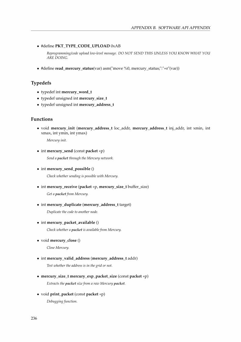
APPENDIX B. SOFTWARE API APPENDIX

• #define PKT_TYPE_CODE_UPLOAD 0xAB

Reprogramming/code upload low-level message. DO NOT SEND THIS UNLESS YOU KNOW WHAT YOUARE DOING.

• #define read_mercury_status(var) asm("move %0, mercury_status;":"=r"(var))

Typedefs

• typedef int mercury_word_t

• typedef unsigned int mercury_size_t

• typedef unsigned int mercury_address_t

Functions

• void mercury_init (mercury_address_t loc_addr, mercury_address_t inj_addr, int xmin, intxmax, int ymin, int ymax)

Mercury init.

• int mercury_send (const packet ∗p)

Send a packet through the Mercury network.

• int mercury_send_possible ()

Check whether sending is possible with Mercury.

• int mercury_receive (packet ∗p, mercury_size_t buffer_size)

Get a packet from Mercury.

• int mercury_duplicate (mercury_address_t target)

Duplicate the code to another node.

• int mercury_packet_available ()

Check whether a packet is available from Mercury.

• void mercury_close ()

Close Mercury.

• int mercury_valid_address (mercury_address_t addr)

Test whether the address is in the grid or not.

• mercury_size_t mercury_exp_packet_size (const packet ∗p)

Extracts the packet size from a raw Mercury packet.

• void print_packet (const packet ∗p)

Debugging function.

236

B.3. MERCURY.H FILE REFERENCE

Variables

• int local_addrAddress constants. They must be initialized correctly at runtime.

• mercury_address_t north_addraddresses for the NSEW neighbors.

• mercury_address_t injection_addrThe address used by the injection point into the grid, to be considered valid !

• mercury_address_t northeast_addrAddresses for the diagonal neighbors.

• int min_addr_xAddress limits. They have to be initialized correctly at runtime to delimit the node grid.

• int grid_xdimUpdated dynamically to store the current Confetti limits.

B.3.1 Source code

1 #ifndef MERCURY_H2 #define MERCURY_H3

4 #include "util.h"5

6 #ifdef TESTING7 #include <stdio.h>8 #include <sys/types.h>9 #include <sys/ipc.h>

10 #include <sys/msg.h>11 #include <errno.h>12 #include <signal.h>13 #include <stdlib .h>14 #include <unistd.h>15 #endif16

17 /∗∗∗∗∗∗∗∗∗∗∗∗∗∗∗∗∗∗∗∗∗∗/18 /∗ PACKET DEFINITIONS ∗/19 /∗∗∗∗∗∗∗∗∗∗∗∗∗∗∗∗∗∗∗∗∗∗/20

21 /∗ primitive types ∗/22 typedef int mercury_word_t; /∗ meant to be 32 bits ∗/23 typedef unsigned int mercury_size_t; /∗ in mercury_word_t words ∗/24 typedef unsigned int mercury_address_t;25

26 /∗ base packet type . might be resized to fit expanding requirements ...27 note that the first two fields must follow the conventions used by the underlying28 bus, ie . Mercury.29

30 Note that lengths and sizes are all in 32−bit words.31

32 Null values for addresses , types and sequence numbers33 mean "undefined" and are used as "any" values in conditional functions .34 ∗/35 typedef struct {36 /∗ fields are inverted in the real Hermes header.37 It seems our MOVE compiler stores bitfields the other way38 We would like them to be , on a 32−bit basis ∗/

237

APPENDIX B. SOFTWARE API APPENDIX

39

40 /∗ ought to be sender | length ∗/41 mercury_size_t length : 16; /∗ implies a maximal message payload of42 64k−1 32−bit words: the header43 takes 1 in this , so this length44 is the real data length + 1.45 This is a Mercury requirement.46 ∗/47 mercury_address_t destination : 16; /∗ implies at most 256 destinations . ∗/48 /∗ ought to be : sender | type | seqnum, inverted to compensate for the compiler ∗/49 unsigned int seqnum : 8;50 unsigned int type : 8; /∗ implies at most 256 packet types ∗/51 mercury_address_t sender : 16; /∗ implies at most 256 senders . ∗/52 mercury_word_t data[0]; /∗ pointer to the beginning of the payload , 32−bit words ∗/53 } __attribute__ ((__packed__)) packet;54

55 /∗ Pack the structure as tight as possible with a __packed__ attribute .56 Very important if the fields are not strictly byte−aligned ∗/57

58 /∗ This length is defined as the length of the data that is not59 taken into consideration in the "length" field of the packet struct .60 Currently , this is 1 − the Mercury header itself only consists of the61 32 first bits of the packet header we use . The rest of the struct is62 specific and its length is taken into account in the length field .63 ∗/64 #define PKT_HEADER_LENGTH 165

66

67 /∗∗∗∗∗∗∗∗∗∗∗∗∗∗∗∗∗/68 /∗ MESSAGE TYPES ∗/69 /∗∗∗∗∗∗∗∗∗∗∗∗∗∗∗∗∗/70

71 /∗ undefined type (means any/none) ∗/72 #define PKT_TYPE_UNDEF 073 /∗ one−way message (needs not be acked) ∗/74 #define PKT_TYPE_ASYNC 175 /∗ synchronous message (needs to be ACKed) ∗/76 #define PKT_TYPE_SYNC 277 /∗ acknowledge for the previous ∗/78 #define PKT_TYPE_ACK 379 /∗ Broadcast with ACKs ∗/80 #define PKT_TYPE_SYNC_BCAST 481 /∗ Broadcast without ACKs ∗/82 #define PKT_TYPE_ASYNC_BCAST 583 /∗ first −level broadcast (send further along the same axis ,84 send second−level broadcast into the other , perpendicular axis )∗/85 #define PKT_TYPE_SYNC_BCAST1 686 /∗ second−level broadcast (send further along the same axis only ∗/87 #define PKT_TYPE_SYNC_BCAST2 788 /∗ first −level broadcast (send further along the same axis ,89 send second−level broadcast into the other , perpendicular axis )∗/90 #define PKT_TYPE_ASYNC_BCAST1 891 /∗ second−level broadcast (send further along the same axis only ∗/92 #define PKT_TYPE_ASYNC_BCAST2 993

94 /∗ reprogramming/code upload low−level message.95 DO NOT SEND THIS UNLESS YOU KNOW WHAT YOU ARE DOING. ∗/96 #define PKT_TYPE_CODE_UPLOAD 0xAB97

98 /∗ Initialize Mercury. This MUST be done before trying anything else .99 Behavior is undefined otherwise .

100

101 ∗/102 void mercury_init(mercury_address_t loc_addr, mercury_address_t inj_addr,103 int xmin, int xmax, int ymin, int ymax);104

105 /∗ Send a packet through the Mercury network.106

238

B.3. MERCURY.H FILE REFERENCE

107 This function waits for the Mercury send buffer to have room, then sends108 the packet proper , possibly blocking if Mercury itself blocks ( full buffer ) .109 A timeout mechanism prevents blocking forever . If this happens, ERROR_TIMEOUT110 is returned , otherwise SUCCESS is returned when the transmission ends.111 ∗/112 int mercury_send(const packet ∗p);113

114 /∗ Check whether sending is possible with Mercury.115 If the Mercury hardware layer reports this is possible , the function returns116 TRUE. Otherwise, it returns FALSE.117 ∗/118 int mercury_send_possible();119

120 /∗ Get a packet from Mercury.121

122 This function waits until a packet is available in the Mercury reception buffer .123 Unless a timeout occurs , in which case it returns ERROR_TIMEOUT, it returns with124 SUCCESS and the packet.This function can also return ERROR_BUFFER in the cases where the125 entire packet is too large to fit in the given buffer size .126 ∗/127 int mercury_receive(packet ∗p, mercury_size_t buffer_size);128

129 /∗ Duplicate the code to another node.130

131 This function sends a packet to the given node that reprograms it with132 the sending node’s code . For this to work, the CODE_BORDER constant has133 to be declared at the beginning of the application code , before all134 relevant includes (even mercury/ confiture ) . All constant arrays and variables135 declared BEFORE it will be sent , but those declared AFTER will be truncated136 at send. ∗/137 int mercury_duplicate(mercury_address_t target);138

139 /∗ Check whether a packet is available from Mercury.140

141 If there is at least one packet in the receive buffer , return TRUE.142 Otherwise, return FALSE.143 ∗/144 int mercury_packet_available();145

146 /∗ Close Mercury.147

148 Of limited use in architectures that do not need to properly "quit"149 an application using Mercury...150 ∗/151 void mercury_close();152

153 /∗ Test whether the address is in the grid or not . ∗/154 int mercury_valid_address(mercury_address_t addr);155

156 mercury_size_t mercury_exp_packet_size(const packet ∗p);157

158

159 /∗∗∗∗∗∗∗∗∗∗∗∗∗∗∗∗∗∗∗/160 /∗ DEBUG FUNCTIONS ∗/161 /∗∗∗∗∗∗∗∗∗∗∗∗∗∗∗∗∗∗∗/162 void print_packet(const packet ∗p);163

164 #ifdef TESTING165 /∗ Called in debug testing when the application gets a SIGINT ∗/166 void clean_exit () ;167 #endif168

169

170 /∗∗∗∗∗∗∗∗∗∗∗∗∗∗∗∗∗∗∗∗∗∗∗∗∗∗∗∗∗∗∗∗∗∗∗∗∗∗∗∗∗∗∗∗∗/171 /∗ CONSTANTS, GLOBAL VARIABLES, BUFFERS, ETC ∗/172 /∗∗∗∗∗∗∗∗∗∗∗∗∗∗∗∗∗∗∗∗∗∗∗∗∗∗∗∗∗∗∗∗∗∗∗∗∗∗∗∗∗∗∗∗∗/173

174 #ifndef TESTING

239

APPENDIX B. SOFTWARE API APPENDIX

175 /∗ hardware−specific constants .176 be careful to update them accordingly if they are changed! ∗/177 #define ACCEPT_DMA_MASK 0x00000001178 #define ALLOW_RECONFIGURATION_MASK 0x00000002179 #define WRITE_IN_PROGRESS_MASK 0x00000004180 #define NEW_DATA_FLAG_MASK 0x00000008181 #define CAN_SEND_DATA_MASK 0x00000010182 #define RECEIVER_EMPTY_DATA_MASK 0x00000020183

184 /∗ hardware defines ∗/185 // sample : asm("move %0, %1":"=r"(dest):"r"(src)) ;186 #define read_mercury_status(var) \187 asm("move %0, mercury_status;":"=r"(var))188 #define read_mercury_pkt_size(var) \189 asm("move %0, mercury_packet_size;":"=r"(var))190 #define read_confiture_header(var) \191 asm("move %0, confiture_header;":"=r"(var))192 #define write_mercury_status(var) \193 asm("move mercury_status, %0;"::"r"(var))194 #define write_mercury_status_val(val) \195 asm("move mercury_status, %0;"::"i"(val))196 #define write_mercury_data(var) \197 asm("move mercury_send_data, %0;"::"r"(var))198 #define write_dma_start_addr(var) \199 asm("move mercury_dma_start_address, %0;"::"r"(var))200 #define write_dma_end_addr(var) \201 asm("move mercury_dma_end_address, %0;"::"r"(var))202 #endif203

204 #define ERROR_TIMEOUT 2205 #define ERROR_BUFFER 3206 #define ERROR_ADDRESS 4207 #define ERROR_NOT_READY 5208 #define ERROR_OVERFLOW 6209

210 /∗ address constants . They must be initialized correctly at runtime ∗/211 int local_addr, local_addr_x, local_addr_y; /∗ address of self ∗/212 /∗ addresses for the NSEW neighbors ∗/213 mercury_address_t north_addr, south_addr, east_addr, west_addr;214

215 /∗ the address used by the injection point into the grid ,216 to be considered valid ! ∗/217 mercury_address_t injection_addr;218

219 // # ifdef MOORE_NEIGHBORHOOD220 /∗ addresses for the diagonal neighbors ∗/221 mercury_address_t northeast_addr, southeast_addr, southwest_addr, northwest_addr;222 // #endif223

224 /∗ address limits . have to be initialized correctly at runtime225 to delimit the node grid . ∗/226 int min_addr_x, max_addr_x, min_addr_y, max_addr_y;227

228 /∗ grid dimensions, computed from the above . ∗/229 int grid_xdim, grid_ydim;230

231 #ifndef TESTING232 /∗ the MOVE GCC has no linker. ∗/233 #include "mercury.c"234 #endif235

236 #endif

Listing B.2: MERCURY API layer.

240

B.4. CONFITURE.H FILE REFERENCE

B.4 Confiture.h File Reference

Data Structures

• struct cond_s

A condition structure used to match packets.

Defines

• #define CONFITURE_MAX_PACKET_SIZE 92

Buffer size in 32-bit words.

• #define CONFITURE_BUFFER_SIZE 16

Buffer size in packets.

Functions

• void confiture_init (mercury_address_t loc_addr, mercury_address_t inj_addr, int xmin, intxmax, int ymin, int ymax)

Initialize the Confiture messaging layer.

• int confiture_try_send (packet ∗p)

Send a packet using Confiture.

• int confiture_receive (packet ∗p, mercury_size_t buffer_size)

Receive a packet using Confiture.

• int confiture_check_receive (packet ∗p, mercury_size_t buffer_size)

Receive a packetp. using Confiture.

• int confiture_wait_packet (packet ∗p, mercury_size_t buffer_size, const cond_s ∗conditions,unsigned int ncond)

Wait for a packet of given type and sequence number, potentially buffering any packetp.structpacket that comesinbetween.

• int confiture_handle_packet_reception (packet ∗p)

Handle a packet’s reception.

• int confiture_propagate_broadcast (packet ∗p)

Propagate broadcast packets according to the algorithm we use.

• int confiture_spread_code ()

Spread code further on the grid.

241

APPENDIX B. SOFTWARE API APPENDIX

B.4.1 Source code

1 #ifndef CONFITURE_H2 #define CONFITURE_H3 #include "mercury.h"4

5 /∗ buffer size in 32−bit words ∗/6 #ifndef CONFITURE_MAX_PACKET_SIZE7 #define CONFITURE_MAX_PACKET_SIZE 928 #endif9

10 /∗ buffer size in packets ∗/11 #ifndef CONFITURE_BUFFER_SIZE12 #define CONFITURE_BUFFER_SIZE 1613 #endif14

15 /∗∗∗∗∗∗∗∗∗∗∗∗∗∗/16 /∗ STRUCTURES ∗/17 /∗∗∗∗∗∗∗∗∗∗∗∗∗∗/18 typedef struct {19 int sender;20 int type;21 int seqnum;22 } cond_s;23

24 /∗∗∗∗∗∗∗∗∗∗∗∗∗∗∗∗∗∗∗∗/25 /∗ PUBLIC FUNCTIONS ∗/26 /∗∗∗∗∗∗∗∗∗∗∗∗∗∗∗∗∗∗∗∗/27 void confiture_init (mercury_address_t loc_addr, mercury_address_t inj_addr,28 int xmin, int xmax, int ymin, int ymax);29

30 /∗ Send a packet using Confiture .31

32 This function is expected to block until : 1. the message could be33 transmitted correctly to the hardware layer , 2. any necessary answers34 have been obtained (ACK messages).35

36 Thus, if the function returns with value SUCCESS, one can be sure the37 message went through. When messages that use acknowledgements are used,38 one can even be sure the application received the message correctly .39

40 Timeouts are implemented to prevent blocking forever in failure cases .41 On such occasions , the function returns ERROR_TIMEOUT.42

43 See confiture_try_send () for a variant that does not wait for the hardware44 layer to be available .45

46 Be aware that the function can modify some fields47 ( destination , sequence number) at will .48 ∗/49 int confiture_send(packet ∗p);50

51 /∗ Send a packet using Confiture .52

53 This function does not wait until the hardware layer is ready , but returns54 FAILURE instead. If the hardware is available , it still waits until all55 proper answers have arrived , though, in which case it returns SUCCESS56 (or ERROR_TIMEOUT if a timeout occured).57

58 Be aware that the function can modify some fields59 ( destination , sequence number) at will .60 ∗/61 int confiture_try_send(packet ∗p);62

63 /∗ Receive a packet using Confiture .64

65 This function is expected to block until : 1. a message has been received ,66 2. the message has been handled by Confiture . Only then the function returns

242

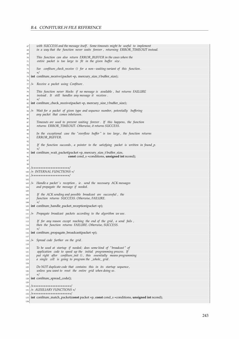
B.4. CONFITURE.H FILE REFERENCE

67 with SUCCESS and the message itself . Some timeouts might be useful to implement68 in a way that the function never waits forever , returning ERROR_TIMEOUT instead.69

70 This function can also return ERROR_BUFFER in the cases where the71 entire packet is too large to fit in the given buffer size .72

73 See confiture_check_receive () for a non−waiting variant of this function .74 ∗/75 int confiture_receive(packet ∗p, mercury_size_t buffer_size);76

77 /∗ Receive a packet using Confiture .78

79 This function never blocks if no message is available , but returns FAILURE80 instead . It still handles any message it receives .81 ∗/82 int confiture_check_receive(packet ∗p, mercury_size_t buffer_size);83

84 /∗ Wait for a packet of given type and sequence number, potentially buffering85 any packet that comes inbetween.86

87 Timeouts are used to prevent waiting forever . If this happens, the function88 returns ERROR_TIMEOUT. Otherwise, it returns SUCCESS.89

90 In the exceptional case the "overflow buffer " is too large , the function returns91 ERROR_BUFFER.92

93 If the function succeeds , a pointer to the satisfying packet is written in found_p.94 ∗/95 int confiture_wait_packet(packet ∗p, mercury_size_t buffer_size,96 const cond_s ∗conditions, unsigned int ncond);97

98

99 /∗∗∗∗∗∗∗∗∗∗∗∗∗∗∗∗∗∗∗∗∗∗/100 /∗ INTERNAL FUNCTIONS ∗/101 /∗∗∗∗∗∗∗∗∗∗∗∗∗∗∗∗∗∗∗∗∗∗/102

103 /∗ Handle a packet ’ s reception , ie . send the necessary ACK messages104 and propagate the message if needed.105

106 If the ACK sending and possible broadcast are successful , the107 function returns SUCCESS. Otherwise, FAILURE.108 ∗/109 int confiture_handle_packet_reception(packet ∗p);110

111 /∗ Propagate broadcast packets according to the algorithm we use .112

113 If for any reason except reaching the end of the grid , a send fails ,114 then the function returns FAILURE. Otherwise, SUCCESS.115 ∗/116 int confiture_propagate_broadcast(packet ∗p);117

118 /∗ Spread code further on the grid .119

120 To be used at startup if needed; does some kind of "broadcast" of121 application code to speed up the initial programming process. If122 put right after confiture_init () , this essentially means programming123 a single cell is going to program the _whole_ grid .124

125 Do NOT duplicate code that contains this in its startup sequence ,126 unless you want to reset the entire grid when doing so .127 ∗/128 int confiture_spread_code();129

130 /∗∗∗∗∗∗∗∗∗∗∗∗∗∗∗∗∗∗∗∗∗∗∗/131 /∗ AUXILIARY FUNCTIONS ∗/132 /∗∗∗∗∗∗∗∗∗∗∗∗∗∗∗∗∗∗∗∗∗∗∗/133 int confiture_match_packet(const packet ∗p, const cond_s ∗conditions, unsigned int ncond);134

243

APPENDIX B. SOFTWARE API APPENDIX

135 int confiture_buffer_empty();136

137 int confiture_find_free_buffer () ;138

139 #ifndef TESTING140 /∗ the MOVE GCC has no linker. ∗/141 #include "confiture.c"142 #endif143

144 #endif

Listing B.3: CONFITURE API layer.

244

B.5. CAFCA CODE SAMPLES

B.5 CAFCA code samples

1 // Spaceship motive2 const int wss1[8][8] = {3 {0,0,0,0,0,0,0,0}, {0,0,0,0,0,0,0,0}, {0,0,0,0,0,0,0,0},4 {0,0,1,1,1,0,0,0}, {0,0,1,1,0,0,1,0}, {0,0,0,0,1,1,1,0},5 {0,0,1,0,0,1,0,1}, {0,1,0,0,0,0,1,0}};6

7 const int wss2[8][8] = {8 {0,0,0,0,0,0,0,0}, {0,0,0,0,0,0,0,0}, {0,0,0,0,0,0,0,0},9 {0,0,0,0,1,0,0,0}, {1,1,0,1,1,0,0,0}, {0,0,0,1,0,0,0,0},

10 {0,0,0,1,0,0,0,0}, {0,0,0,1,0,0,0,0}};11

12 const int wss3[8][8] = {13 {0,1,0,0,0,0,1,0}, {0,0,1,0,0,1,0,1}, {0,0,0,0,1,1,1,0},14 {0,0,1,1,0,0,1,0}, {0,0,1,1,1,0,0,0}, {0,0,0,0,0,0,0,0},15 {0,0,0,0,0,0,0,0}, {0,0,0,0,0,0,0,0}};16

17 const int wss4[8][8] = {18 {0,0,0,1,0,0,0,0}, {0,0,0,1,0,0,0,0}, {0,0,0,1,0,0,0,0},19 {1,1,0,1,1,0,0,0}, {0,0,0,0,1,0,0,0}, {0,0,0,0,0,0,0,0},20 {0,0,0,0,0,0,0,0}, {0,0,0,0,0,0,0,0}};21

22 const int CODE_BORDER = 0;23

24 #include "../cafca/cafca.h" /∗ compile with −DMOORE_NEIGHBORHOOD ∗/25

26 #ifdef TESTING27 #include <stdio.h>28 #include <stdlib .h>29 #include <assert .h>30 #endif31

32 /∗ Grid dimensions ∗/33 #ifdef TESTING34 #define MIN_X 135 #define MAX_X 336 #define MIN_Y 137 #define MAX_Y 338 #else39 #define MIN_X 140 #define MAX_X 641 #define MIN_Y 142 #define MAX_Y 643 #endif44

45 /∗ " injection " address for an interface outside the grid ∗/46 #define INJECTION_ADDR 0x000147

48 int state [8][8], new_state[8][8], north_state [8][8], east_state [8][8], west_state [8][8], south_state [8][8],49 northeast_state [8][8], southeast_state [8][8], southwest_state[8][8], northwest_state [8][8];50

51 /∗ Get a neighbor ∗/52 int neighbour8_wrapping(int i, int j) {53 if ( i<0) {54 if ( j < 0) return northwest_state[8+i][8+j ];55 if ( j > 7) return northeast_state[8+i ][ j−8];56 return north_state[8+i ][ j ];57 }58 if ( i>7) {59 if ( j < 0) return southwest_state[i−8][8+j];60 if ( j > 7) return southeast_state[ i−8][j−8];61 return south_state[i−8][j ];62 }63 if ( j<0) return west_state[i][8+ j ];64 if ( j>7) return east_state [ i ][ j−8];65 return state [ i ][ j ];

245

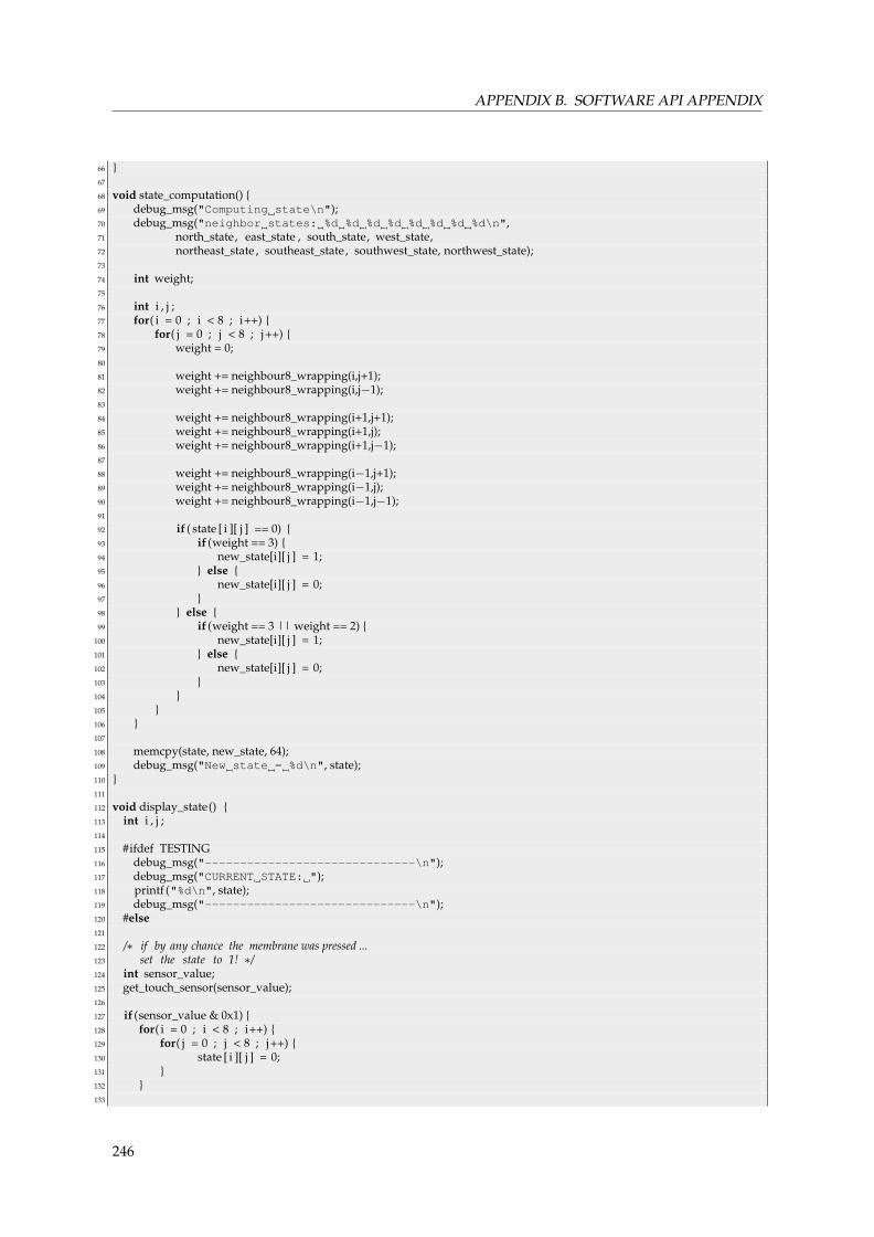
APPENDIX B. SOFTWARE API APPENDIX

66 }67

68 void state_computation() {69 debug_msg("Computing state\n");70 debug_msg("neighbor states: %d %d %d %d %d %d %d %d\n",71 north_state, east_state , south_state, west_state,72 northeast_state , southeast_state, southwest_state, northwest_state);73

74 int weight;75

76 int i , j ;77 for( i = 0 ; i < 8 ; i++) {78 for( j = 0 ; j < 8 ; j++) {79 weight = 0;80

81 weight += neighbour8_wrapping(i,j+1);82 weight += neighbour8_wrapping(i,j−1);83

84 weight += neighbour8_wrapping(i+1,j+1);85 weight += neighbour8_wrapping(i+1,j);86 weight += neighbour8_wrapping(i+1,j−1);87

88 weight += neighbour8_wrapping(i−1,j+1);89 weight += neighbour8_wrapping(i−1,j);90 weight += neighbour8_wrapping(i−1,j−1);91

92 if ( state [ i ][ j ] == 0) {93 if (weight == 3) {94 new_state[i][ j ] = 1;95 } else {96 new_state[i][ j ] = 0;97 }98 } else {99 if (weight == 3 || weight == 2) {

100 new_state[i][ j ] = 1;101 } else {102 new_state[i][ j ] = 0;103 }104 }105 }106 }107

108 memcpy(state, new_state, 64);109 debug_msg("New state = %d\n", state);110 }111

112 void display_state() {113 int i , j ;114

115 #ifdef TESTING116 debug_msg("------------------------------\n");117 debug_msg("CURRENT STATE: ");118 printf ("%d\n", state);119 debug_msg("------------------------------\n");120 #else121

122 /∗ if by any chance the membrane was pressed ...123 set the state to 1! ∗/124 int sensor_value;125 get_touch_sensor(sensor_value);126

127 if (sensor_value & 0x1) {128 for( i = 0 ; i < 8 ; i++) {129 for( j = 0 ; j < 8 ; j++) {130 state [ i ][ j ] = 0;131 }132 }133

246

B.5. CAFCA CODE SAMPLES

134 // GLIDER135 state [3][3] = 0; state [3][4] = 1; state [3][5] = 0; state [4][3] = 0;136 state [4][4] = 0; state [4][5] = 1; state [5][3] = 1; state [5][4] = 1;137 state [5][5] = 1;138

139 // ACORN140 /∗const int acorn [8][8] = {141 {0,0,0,0,0,0,0,0},142 {0,0,0,0,0,0,0,0},143 {0,0,1,0,0,0,0,0},144 {0,0,0,0,1,0,0,0},145 {0,1,1,0,0,1,1,1},146 {0,0,0,0,0,0,0,0},147 {0,0,0,0,0,0,0,0},148 {0,0,0,0,0,0,0,0}149 }; ∗/150

151 // memcpy(state, acorn, 64) ;152 }153

154 #ifndef DEBUG155 for( i = 0 ; i < 8 ; i++) {156 for( j = 0 ; j < 8 ; j++) {157 display(RED_PLANE + i∗8 + j, state[i][j]∗255) ;158 display(BLUE_PLANE + i∗8 + j, state[i][j]∗255) ;159 }160 }161 #endif162

163 #endif164 }165

166 void init () {167 int i , j ;168 for( i = 0 ; i < 8 ; i++) {169 for( j = 0 ; j < 8 ; j++) {170 state [ i ][ j ] = 0;171 }172 }173

174 // Copy the initial pattern175 if (local_addr == 0x0302)176 memcpy(state, wss1, 64);177 else if (local_addr == 0x0402)178 memcpy(state, wss2, 64);179 else if (local_addr == 0x0301)180 memcpy(state, wss3, 64);181 else if (local_addr == 0x0401)182 memcpy(state, wss4, 64);183

184 clear_screen() ;185

186 /∗ set CAFCA constants the way it ought to be ∗/187 app_state_size = 64;188

189 app_state = (mercury_word_t∗) state;190 app_neighbor_states[0] = (mercury_word_t∗) north_state;191 app_neighbor_states[1] = (mercury_word_t∗) east_state;192 app_neighbor_states[2] = (mercury_word_t∗) south_state;193 app_neighbor_states[3] = (mercury_word_t∗) west_state;194 app_neighbor_states[4] = (mercury_word_t∗) northeast_state;195 app_neighbor_states[5] = (mercury_word_t∗) southeast_state;196 app_neighbor_states[6] = (mercury_word_t∗) southwest_state;197 app_neighbor_states[7] = (mercury_word_t∗) northwest_state;198

199 // Sets the display and state functions used by the CAFCA API200 app_state_computation = &state_computation;201 app_state_display = &display_state;

247

APPENDIX B. SOFTWARE API APPENDIX

202 }203

204 void main() {205 cafca_init (0, 0x0101, &init, INJECTION_ADDR, MIN_X, MAX_X, MIN_Y, MAX_Y);206

207 // Self− replicate the code208 if (local_addr == 0x0202)209 {210 confiture_spread();211 }212

213 cafca_main_loop();214 cafca_close () ;215 }

Listing B.4: Sample code for Game-of-life implemented with CAFCA.

1 // available values : jet512 , hot5122 #ifdef JET_PALETTE3 #define PALETTE jet5124 #include "../common/jet512.c"5 #else6 #define PALETTE hot5127 #include "../common/hot512.c"8 #endif9

10 const int CODE_BORDER = 0;11

12 #include "../cafca/cafca.h" /∗ compile with −DMOORE_NEIGHBORHOOD ∗/13 #ifdef TESTING14 #include <stdio.h>15 #include <stdlib .h>16 #include <assert .h>17 #endif18

19 /∗ Grid dimensions ∗/20 #ifdef TESTING21 #define MIN_X 122 #define MAX_X 323 #define MIN_Y 124 #define MAX_Y 325 #else26 #define MIN_X 127 #define MAX_X 628 #define MIN_Y 129 #define MAX_Y 630 #endif31

32 /∗ " injection " address for an interface outside the grid ∗/33 #define INJECTION_ADDR 0x000134

35 // Heat constants36 #define DISSIPATION 110037

38 // Used to slow down the computation of the new states39 // 0 is maximum speed40 #define SLOWDOWN_FACTOR 241

42 int state [8][8], new_state[8][8], north_state [8][8], east_state [8][8], west_state [8][8], south_state [8][8],43 northeast_state [8][8], southeast_state [8][8], southwest_state[8][8], northwest_state [8][8];44

45 // Border condition where we simply copy the state of the border when pertinent46 int get_copy(int i , int j ) {47

48 if ( i<0) {49 if (local_addr_y == MAX_Y) {50 return state [0][ j ];51 }

248

B.5. CAFCA CODE SAMPLES

52 else53 {54 if ( j < 0)55 {56 if (local_addr_x == MIN_X)57 return state [0][0];58 else59 return northwest_state[8+i][8+j ];60 }61 if ( j > 7)62 {63 if (local_addr_x == MAX_X)64 return state [0][7];65 else66 return northeast_state[8+i ][ j−8];67 }68 return north_state[8+i ][ j ];69 }70 }71

72 if ( i>7){73 if (local_addr_y == MIN_Y) {74 return state [7][ j ];75 }76 else77 {78 if ( j < 0)79 {80 if (local_addr_x == MIN_X)81 return state [7][0];82 else83 return southwest_state[i−8][8+j];84 }85 if ( j > 7)86 {87 if (local_addr_x == MAX_X)88 return state [7][7];89 else90 return southeast_state[ i−8][j−8];91

92 // Random, comrade. Random.93 set_seed(local_addr);94 }95

96 return south_state[i−8][j ];97 }98 }99

100 if ( j<0) {101 if (local_addr_x == MIN_X)102 return state [ i ][0];103 else104 return west_state[i][8+ j ];105 }106

107 if ( j>7) {108 if (local_addr_x == MAX_X)109 return state [ i ][7];110 else111 return east_state [ i ][ j−8];112 }113 return state [ i ][ j ];114 }115

116 // Border condition with toroidal wrapping117 int get64(int i , int j ) {118 if ( i<0) {119 if ( j < 0) return northwest_state[8+i][8+j ];

249

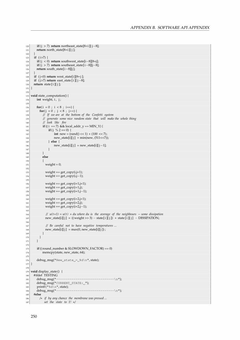
APPENDIX B. SOFTWARE API APPENDIX

120 if ( j > 7) return northeast_state[8+i ][ j−8];121 return north_state[8+i ][ j ];122 }123 if ( i>7) {124 if ( j < 0) return southwest_state[i−8][8+j];125 if ( j > 7) return southeast_state[ i−8][j−8];126 return south_state[i−8][j ];127 }128 if ( j<0) return west_state[i][8+ j ];129 if ( j>7) return east_state [ i ][ j−8];130 return state [ i ][ j ];131 }132

133 void state_computation() {134 int weight, i , j ;135

136 for( i = 0 ; i < 8 ; i++) {137 for( j = 0 ; j < 8 ; j++) {138 // If we are at the bottom of the Confetti system139 // generate some nice random state that will make the whole thing140 // look like fire141 if (( i == 7) && local_addr_y == MIN_Y) {142 if ( j % 2 == 0) {143 int new = (rand() << 1) + (100 << 7);144 new_state[i][ j ] = min(new, (511<<7));145 } else {146 new_state[i][ j ] = new_state[i][ j−1];147 }148 }149 else150 {151 weight = 0;152

153 weight += get_copy(i,j+1);154 weight += get_copy(i,j−1);155

156 weight += get_copy(i+1,j+1);157 weight += get_copy(i+1,j);158 weight += get_copy(i+1,j−1);159

160 weight += get_copy(i+2,j+1);161 weight += get_copy(i+2,j);162 weight += get_copy(i+2,j−1);163

164 // u(t+1) = u(t ) + du where du is the average of the neighbours − some dissipation165 new_state[i][ j ] = ((weight >> 3) − state[ i ][ j ]) + state [ i ][ j ] − DISSIPATION;166

167 // Be careful not to have negative temperatures ...168 new_state[i][ j ] = max(0, new_state[i][ j ]) ;169 }170 }171 }172

173 if (( round_number & SLOWDOWN_FACTOR) == 0)174 memcpy(state, new_state, 64);175

176 debug_msg("New state = %d\n", state);177 }178

179 void display_state() {180 #ifdef TESTING181 debug_msg("------------------------------\n");182 debug_msg("CURRENT STATE: ");183 printf ("%d\n", state);184 debug_msg("------------------------------\n");185 #else186 /∗ if by any chance the membrane was pressed ...187 set the state to 1! ∗/

250

B.5. CAFCA CODE SAMPLES

188 int sensor_value;189 int i , j ;190 get_touch_sensor(sensor_value);191

192 // make things a bit more random at the bottom (rand. button presses )193 if (( sensor_value & 0x1) || ((local_addr_y == min_addr_y) && (rand() < 327))) {194 state [3][3] = 0 xffff ;195 state [4][4] = 0 xffff ;196 state [3][4] = 0 xffff ;197 state [4][3] = 0 xffff ;198 state [2][3] = 0xfd00;199 state [2][4] = 0xfd00;200 state [3][2] = 0xfd00;201 state [4][2] = 0xfd00;202 state [3][5] = 0xfd00;203 state [4][5] = 0xfd00;204 state [5][3] = 0xfd00;205 state [5][4] = 0xfd00;206 state [2][2] = 0xf000;207 state [2][5] = 0xf000;208 state [5][2] = 0xf000;209 state [5][5] = 0xf000;210 }211

212 #ifndef DEBUG213 int color_bias ;214 if (local_addr_y > 3)215 color_bias = 64;216 else217 color_bias = 0;218

219 for( i = 0 ; i < 8 ; i++) {220 for( j = 0 ; j < 8 ; j++) {221 int clr = state [ i ][ j ] >> 7;222

223 int pos = i∗8 + j ;224

225 int red = max(((signed) PALETTE[clr][0]) − color_bias, 0);226 int green = max(((signed) PALETTE[clr][1]) − color_bias, 0);227 int blue = max(((signed) PALETTE[clr][2]) − color_bias, 0);228 display(RED_PLANE + pos, red);229 display(GREEN_PLANE + pos, green);230 display(BLUE_PLANE + pos, blue);231 }232 }233 #endif234 #endif235 }236

237 void init () {238 debug_msg("HELLO WORLD, INIT\n");239

240 clear_screen() ;241

242 // initialize the state as empty243 int i , j ;244 for( i = 0 ; i < 8 ; i++) {245 for( j = 0 ; j < 8 ; j++) {246 state [ i ][ j ] = 0;247 }248 }249

250 /∗ set CAFCA constants the way they ought to be ∗/251 app_state_size = 64;252

253 app_state = (mercury_word_t∗) state;254 app_neighbor_states[0] = (mercury_word_t∗) north_state;255 app_neighbor_states[1] = (mercury_word_t∗) east_state;

251

APPENDIX B. SOFTWARE API APPENDIX

256 app_neighbor_states[2] = (mercury_word_t∗) south_state;257 app_neighbor_states[3] = (mercury_word_t∗) west_state;258 app_neighbor_states[4] = (mercury_word_t∗) northeast_state;259 app_neighbor_states[5] = (mercury_word_t∗) southeast_state;260 app_neighbor_states[6] = (mercury_word_t∗) southwest_state;261 app_neighbor_states[7] = (mercury_word_t∗) northwest_state;262

263 // Sets the function that computes the next state264 app_state_computation = &state_computation;265

266 // And the display function267 app_state_display = &display_state;268

269 // Random, comrade. Random.270 set_seed(local_addr);271 }272

273 void main() {274 cafca_init (0, 0x0101, &init, INJECTION_ADDR, MIN_X, MAX_X, MIN_Y, MAX_Y);275

276 // Self− replication of the code277 if (local_addr == 0x0202) {278 confiture_spread();279 }280

281 cafca_main_loop();282 cafca_close () ;283 }

Listing B.5: Sample code for fire effect implemented with CAFCA.

252

B.6. SOFTWARE ARCHITECTURE OF THE GUI

B.6 Software architecture of the GUI

parasitix

GraphEditor.javaPConstants.java

confetti

ConfettiSocketInterface.javaConfettiState.javaConfettiStats.java

environment

SimpleEnvironment.javaSimulationApp.java

plots

JConfettiPerformancePlot.javaJGlobalPerformancePlot.java

JTaskStatusPlot.javaJVCCPlot.java

prefuse

GraphUtilities.java

simulation

Simulatable.javaSimulator.java

StackSimulator.java

substrate

Mesh2D.javaTopology.java

taskgraph

GraphicTaskGraph.javaGraphicTaskGraphLoader.java

tasks

IOStack.javaNonExistingTaskException.java

PerfCounter.javaSimpleTasks.java

State.javaTask.java

TaskGraph.javaTaskManager.java

tests

GraphModificationsTest.java

ui

JSliderValue.javaPopupMenuController.javaSimulationAppState.java

util

Pastels.javaResourceLocator.javaStatDumper.java

visualization

GraphVisulalizer.javaMapperPanel.java

confetti.actions

ConfettiUploadAction.javaGenerateSSSPGraphFileAction.java

MapGraphToGridAction.javaSenderRateChangedAction.java

updaters

GlobalPerformancePlotUpdater.javaTaskPlotUpdater.java

plots_actions

plots.actions

IOChannelColorAction.javaMapToGridAction.javaNodeColorAction.java

SizeResettingAnimator.java

activity

UpdateListener.java

data

CGraph.java

renderers

ComplexEdgeRenderer.javaIOChannelRenderer.javaTaskRenderer.java

utils

real

ExecutionEnvironment.javaExecutor.javaGenerator.javaRemover.java

samplegraphs

EmptyGraph.javaExampleGraph.javaGraphTypes.java

LineTasksGraph.javaMeshTaskGraph.javaTrivialGraph.java

channels

Channel.javaInputChannel.java

NoDelayChannel.javaOutputChannel.javaPeriodicChannel.java

manager

CentralizedGluttonousManager.javaDistributedGluttonousManager.java

muxes

Demultiplexer.javaMultiplexer.java

streams

RandomDataStreamsNormalDataStream.java

ui.actions

ActionConstants.javaCreateGlobalPerformancePlotAction.java

CreateTaskDialogAction.javaDeleteTaskDialogAction.java

InstanciateNewGraphAction.javaInstanciateVCCGrapherAction.javaInstanciateNewChannelAction.javaInstanciateNewTaskAction.javaLayoutGraphAsATreeAction.java

LoadGraphAction.javaRemoveTaskFromGraphAction.java

SaveGraphAction.javaSaveTaskAction.java

ToggleSimulationRunningAction.java

menu

JExtendedMenu.javaMenuFactory.java

panels

JChannelEditor.javaJClockPanel.java

JComponentChooserPanel.javaJForcePanel.java

JMapperControlPanel.javaJMapperPanel.java

JSimulationControlPanel.javaJTaskChooserPanel.javaJTaskEditorPanel.java

JTaskInfoDisplayPanel.java

toolbars

ToolBarFactory.java

force

GridWellForce.java

Figure B.1: Software architecture of the GUI.

253

APPENDIX B. SOFTWARE API APPENDIX

B.7 CAFCA task code template

1 /∗2 ∗∗ CAFCA Template3 ∗∗ For simulation only :4 ∗∗ Beware that every global variable declared here lies in the5 ∗∗ shared segment of the thread , which means that every task that implements6 ∗∗ this task has access to the SAME memory. Hence, every global data is7 ∗∗ shared among the instances of the thread .8 ∗∗9 ∗∗ Pierre−Andre Mudry, EPFL, 2008

10 ∗∗/11 #include "TASK_NAME.h"12 #include "stdio.h"13

14 // available values : jet512 , hot51215 #ifdef JET_PALETTE16 #define PALETTE jet51217 #include "../common/jet512.c"18 #else19 #define PALETTE hot51220 #include "../common/hot512.c"21 #endif22

23 const int CODE_BORDER = 0;24

25 #include "../cafca/cafca.h" /∗ compile with −DMOORE_NEIGHBORHOOD ∗/26

27 int state [8][8], new_state[8][8], north_state [8][8], east_state [8][8], west_state [8][8], south_state [8][8],28 northeast_state [8][8], southeast_state [8][8], southwest_state[8][8], northwest_state [8][8];29

30 /∗31 ∗ CAFCA task execution function32 ∗/33 void state_computation() {34 // TODO Insert your state computation code here35 int weight, i , j ;36

37 for( i = 0 ; i < 8 ; i++) {38 for( j = 0 ; j < 8 ; j++) {39 new_state[i][ j ] = 0;40 }41 }42

43 memcpy(state, new_state, 64);44 }45

46 // Entry point for the task when executed in the simulation environment47 #ifdef _SIM48 void init () {49 // Initialize the state as empty50 int i , j ;51 for( i = 0 ; i < 8 ; i++) {52 for( j = 0 ; j < 8 ; j++) {53 state [ i ][ j ] = 0;54 }55 }56

57 /∗ set CAFCA constants the way they ought to be ∗/58 app_state_size = 64;59

60 app_state = (mercury_word_t∗) state;61 app_neighbor_states[0] = (mercury_word_t∗) north_state;62 app_neighbor_states[1] = (mercury_word_t∗) east_state;63 app_neighbor_states[2] = (mercury_word_t∗) south_state;64 app_neighbor_states[3] = (mercury_word_t∗) west_state;65 app_neighbor_states[4] = (mercury_word_t∗) northeast_state;

254

B.7. CAFCA TASK CODE TEMPLATE

66 app_neighbor_states[5] = (mercury_word_t∗) southeast_state;67 app_neighbor_states[6] = (mercury_word_t∗) southwest_state;68 app_neighbor_states[7] = (mercury_word_t∗) northwest_state;69 }70

71 void ∗task_init (void ∗taskParameters)72 {73 byte db = 0;74 int status = C_NOCOMMAND;75

76 stack instack , outstack;77 sTask_init ∗ initParams = (sTask_init ∗)taskParameters;78

79 memset(instack.buffer, 0, BUFSIZE);80 instack . level = 0;81 instack .socket = 0;82 instack .command = C_NOCOMMAND;83 instack .port = initParams−>inPort;84

85 memset(outstack.buffer, 0, BUFSIZE);86 outstack. level = 0;87 outstack.socket = 0;88 outstack.command = C_NOCOMMAND;89 outstack.port = initParams−>outPort;90

91 init_sim_lib(&instack, &outstack);92

93 printf ("CAFCA Task created, name is %s, listening on port : %d and sending to port %d\n",initParams−>taskname, instack.port, outstack.port);

94

95 while(1)96 {97 status = getStackStatus(&instack);98

99 // If data present in input stack100 if (status != C_NOCOMMAND)101 {102 printf ("command received %x\n", status);103 }104 else if (! inputEmpty(&instack))105 {106 // Read data chunk107 db = popInput(&instack);108

109 // Wait until output stack can accept new data110 while(outputFull()) {};111

112 // Push the result113 pushOutput(state_computation(), &outstack);114 }115

116 // If simulated in a windows environment, sleep117 #ifdef _WIN32118 Sleep(1) ;119 #endif120 }121

122 pthread_exit(NULL);123 }124 #endif125

126 // Entry point for the task when executed in a standalone environment127 #ifdef _PROFILING128

129 void init () {130 // Initialize the state as empty131 int i , j ;132 for( i = 0 ; i < 8 ; i++) {

255

APPENDIX B. SOFTWARE API APPENDIX

133 for( j = 0 ; j < 8 ; j++) {134 state [ i ][ j ] = 0;135 }136 }137

138 /∗ set CAFCA constants the way they ought to be ∗/139 app_state_size = 64;140

141 app_state = (mercury_word_t∗) state;142 app_neighbor_states[0] = (mercury_word_t∗) north_state;143 app_neighbor_states[1] = (mercury_word_t∗) east_state;144 app_neighbor_states[2] = (mercury_word_t∗) south_state;145 app_neighbor_states[3] = (mercury_word_t∗) west_state;146 app_neighbor_states[4] = (mercury_word_t∗) northeast_state;147 app_neighbor_states[5] = (mercury_word_t∗) southeast_state;148 app_neighbor_states[6] = (mercury_word_t∗) southwest_state;149 app_neighbor_states[7] = (mercury_word_t∗) northwest_state;150 }151

152 void main()153 {154 // TODO Replace with your own profiling code155 int i = 0;156

157 init () ;158

159 for( i = 0; i < 10000000; i++)160 {161 state_computation();162 }163 }164 #endif165

166 // Entry point for the task when executed in a standalone environment167 #ifdef _REAL168 void display_state() {169

170 // TODO Insert the code to display the state here171 int sensor_value;172 int i , j ;173

174 /∗ if by any chance the membrane was pressed ...175 set the state to 1! ∗/176 get_touch_sensor(sensor_value);177

178 if (sensor_value & 0x1)179 state [3][3] = 0 xffff ;180 state [4][4] = 0 xffff ;181 state [3][4] = 0 xffff ;182 state [4][3] = 0 xffff ;183 }184

185 // Display the cell state using a palette186 for( i = 0 ; i < 8 ; i++) {187 for( j = 0 ; j < 8 ; j++) {188 int clr = state [ i ][ j ] >> 7;189 int pos = i∗8 + j ;190

191 int red = max(((signed) PALETTE[clr][0]) − color_bias, 0);192 int green = max(((signed) PALETTE[clr][1]) − color_bias, 0);193 int blue = max(((signed) PALETTE[clr][2]) − color_bias, 0);194 display(RED_PLANE + pos, red);195 display(GREEN_PLANE + pos, green);196 display(BLUE_PLANE + pos, blue);197 }198 }199 }200

256

B.7. CAFCA TASK CODE TEMPLATE

201 void init () {202 // TODO Change the init function to store the state size or use different neighborhood ...203 clear_screen() ;204

205 // Initialize the state as empty206 int i , j ;207 for( i = 0 ; i < 8 ; i++) {208 for( j = 0 ; j < 8 ; j++) {209 state [ i ][ j ] = 0;210 }211 }212

213 /∗ set CAFCA constants the way they ought to be ∗/214 app_state_size = 64;215

216 app_state = (mercury_word_t∗) state;217 app_neighbor_states[0] = (mercury_word_t∗) north_state;218 app_neighbor_states[1] = (mercury_word_t∗) east_state;219 app_neighbor_states[2] = (mercury_word_t∗) south_state;220 app_neighbor_states[3] = (mercury_word_t∗) west_state;221 app_neighbor_states[4] = (mercury_word_t∗) northeast_state;222 app_neighbor_states[5] = (mercury_word_t∗) southeast_state;223 app_neighbor_states[6] = (mercury_word_t∗) southwest_state;224 app_neighbor_states[7] = (mercury_word_t∗) northwest_state;225

226 // Sets the function that computes the next state227 app_state_computation = &state_computation;228

229 // And the display function230 app_state_display = &display_state;231

232 // Random, comrade. Random.233 set_seed(local_addr);234 }235

236 void main() {237 cafca_init (0, 0x0101, &init, INJECTION_ADDR, MIN_X, MAX_X, MIN_Y, MAX_Y);238

239 // Self− replication of the code ( if required )240 if (local_addr == 0x0202) {241 confiture_spread();242 }243

244 // Call CAFCA main loop245 cafca_main_loop();246 cafca_close () ;247 }248 #endif

Listing B.6: Code template for a CAFCA task.

257

APPENDIX B. SOFTWARE API APPENDIX

B.8 SSSP task code template

1 /∗∗2 ∗∗ SSSP code TEMPLATE3 ∗∗4 ∗∗ For simulation only :5 ∗∗ Beware that every global variable declared here lies in the6 ∗∗ shared segment of the thread , which means that every task that implements7 ∗∗ this task has access to the SAME memory. Hence, every global data is8 ∗∗ shared among the instances of the thread .9 ∗∗

10 ∗∗ Pierre−Andre Mudry, EPFL, 200811 ∗∗/12

13 #include "TASK_NAME.h"14 #include "stdio.h"15

16 const int CODE_BORDER = 0;17

18 #include "stream/stream.h"19

20 // The task ’ s execution function21 int compute(int val)22 {23 // TODO Replace with your own code24 int result = val + 2;25 return result ;26 }27

28 // Entry point for the task when executed in the simulation environment29 #ifdef _SIM30 void ∗task_init (void ∗taskParameters)31 {32 byte db = 0;33 int status = C_NOCOMMAND;34

35 stack instack , outstack;36 sTask_init ∗ initParams = (sTask_init ∗)taskParameters;37

38 memset(instack.buffer, 0, BUFSIZE);39 instack . level = 0;40 instack .socket = 0;41 instack .command = C_NOCOMMAND;42 instack .port = initParams−>inPort;43

44 memset(outstack.buffer, 0, BUFSIZE);45 outstack. level = 0;46 outstack.socket = 0;47 outstack.command = C_NOCOMMAND;48 outstack.port = initParams−>outPort;49

50 init_sim_lib(&instack, &outstack);51

52 printf ("Task created, name is %s, listening on port : %d and sending to port %d\n", initParams−>taskname, instack.port, outstack.port);

53

54 while(1)55 {56 status = getStackStatus(&instack);57

58 // If data present in input stack59 if (status != C_NOCOMMAND)60 {61 printf ("command received %x\n", status);62 }63 else if (! inputEmpty(&instack))64 {

258

B.8. SSSP TASK CODE TEMPLATE

65 // Read data chunk66 db = popInput(&instack);67

68 // Wait until output stack can accept new data69 while(outputFull()) {};70

71 // Push the result72 pushOutput(compute(db), &outstack);73 }74

75 // If simulated in a windows environment, sleep76 #ifdef _WIN3277 Sleep(1) ;78 #endif79 }80

81 pthread_exit(NULL);82 }83 #endif84

85 // Entry point for the task when executed in a standalone environment86 #ifdef _PROFILING87 void main()88 {89 // TODO Replace with your own profiling code90 int i = 0;91

92 for( i = 0; i < 10000000; i++)93 {94 compute(i);95 }96 }97 #endif98

99 // Entry point for the task when executed in SSSP environment100 #ifdef _REAL101 void computation(job ∗j) {102 // TODO Replace with your own code103 my_job ∗aj = (my_job∗) j−>data; // Cast the job type .104

105 // TODO Do you processing here106 compute(YOUR_DATA);107

108 // Display.109 #ifdef DEBUG110 display_bin(aj−>state[DEBUG_POS], GREEN_PLANE+32);111 #endif112

113 // Correct the job type .114 j−>type = app_destination_gids[0];115

116 // Send as−is. The sender is automatically corrected by117 // the send() function .118 stream_output(j);119 }120

121 void init () {122 app_computation = &computation;123 stream_status_array = status_array;124 }125

126 void main() {127 stream_init(INJECTION_ADDR, MIN_X, MAX_X, MIN_Y, MAX_Y, &init);128 stream_main_loop();129 }130 #endif

Listing B.7: Code template for a SSSP task.

259

List of Tables

3.1 Embedded memory controller memory map. . . . . . . . . . . . . . . . . . . . . . . . . . 383.2 SRAM FU Interface. . . . . . . . . . . . . . . . . . . . . . . . . . . . . . . . . . . . . . . . . 423.3 Arithmetic FUs available for the ULYSSE processor. . . . . . . . . . . . . . . . . . . . . . . 433.4 Condition functional unit. . . . . . . . . . . . . . . . . . . . . . . . . . . . . . . . . . . . . 443.5 ALU functional unit. . . . . . . . . . . . . . . . . . . . . . . . . . . . . . . . . . . . . . . . 453.6 Size and speed of available ULYSSE functional units. . . . . . . . . . . . . . . . . . . . . . 46

4.1 Tokenization of the input file. . . . . . . . . . . . . . . . . . . . . . . . . . . . . . . . . . . . 53

5.1 Performance measures on various programs. . . . . . . . . . . . . . . . . . . . . . . . . . 795.2 Code size measurements. . . . . . . . . . . . . . . . . . . . . . . . . . . . . . . . . . . . . 805.3 Simulation and execution times. . . . . . . . . . . . . . . . . . . . . . . . . . . . . . . . . . 81

6.1 Evolution results on various programs (mean value of 500 runs). . . . . . . . . . . . . . . 98

7.1 Cell board I/O signals. . . . . . . . . . . . . . . . . . . . . . . . . . . . . . . . . . . . . . . 109

8.1 Mercury FU memory map. . . . . . . . . . . . . . . . . . . . . . . . . . . . . . . . . . . . . 1278.2 Display FU memory map. . . . . . . . . . . . . . . . . . . . . . . . . . . . . . . . . . . . . 128

A.1 ALU functional unit memory map. . . . . . . . . . . . . . . . . . . . . . . . . . . . . . . . 206A.2 Parallel shifter memory map. . . . . . . . . . . . . . . . . . . . . . . . . . . . . . . . . . . 206A.3 Concatenation unit memory map. . . . . . . . . . . . . . . . . . . . . . . . . . . . . . . . . 206A.4 Condition functional unit memory map. . . . . . . . . . . . . . . . . . . . . . . . . . . . . 207A.5 GPIO functional unit memory map. . . . . . . . . . . . . . . . . . . . . . . . . . . . . . . 207A.6 Mercury FU memory map. . . . . . . . . . . . . . . . . . . . . . . . . . . . . . . . . . . . . 207A.7 Display FU memory map. . . . . . . . . . . . . . . . . . . . . . . . . . . . . . . . . . . . . 208A.8 Timer FU memory map. . . . . . . . . . . . . . . . . . . . . . . . . . . . . . . . . . . . . . 208A.9 SRAM FU Interface memory map. . . . . . . . . . . . . . . . . . . . . . . . . . . . . . . . 208A.10 Assertion FU memory map. . . . . . . . . . . . . . . . . . . . . . . . . . . . . . . . . . . . 209A.11 Divider unit memory map. . . . . . . . . . . . . . . . . . . . . . . . . . . . . . . . . . . . . 209

261

List of Figures

2.1 Separation of hardware-software responsibilities for some processor architectures. . . 152.2 VLIW instruction word specification in TTA. . . . . . . . . . . . . . . . . . . . . . . . . 162.3 General architecture of a TTA processor. . . . . . . . . . . . . . . . . . . . . . . . . . . . 17

3.1 Overview of a minimal ULYSSE processor. . . . . . . . . . . . . . . . . . . . . . . . . . . 283.2 Schematic TTA adder example. . . . . . . . . . . . . . . . . . . . . . . . . . . . . . . . . 293.3 Detailed view of the ULYSSE processor in its standalone version. . . . . . . . . . . . . . 313.4 Schematic of the common bus interface. . . . . . . . . . . . . . . . . . . . . . . . . . . . 333.5 Fetch unit state machine. . . . . . . . . . . . . . . . . . . . . . . . . . . . . . . . . . . . . 343.6 The fetch unit. . . . . . . . . . . . . . . . . . . . . . . . . . . . . . . . . . . . . . . . . . . 353.7 The SRAM controller FU schematic. . . . . . . . . . . . . . . . . . . . . . . . . . . . . . 393.8 Fetch unit state-machine when using external SRAM memory. . . . . . . . . . . . . . . 403.9 SRAM controller timings. . . . . . . . . . . . . . . . . . . . . . . . . . . . . . . . . . . . 413.10 ULYSSE functional units hierarchy. . . . . . . . . . . . . . . . . . . . . . . . . . . . . . . 433.11 MACC with permanent connections. . . . . . . . . . . . . . . . . . . . . . . . . . . . . . 47

4.1 Description of the various phases of assembly. . . . . . . . . . . . . . . . . . . . . . . . 524.2 Decorated syntactic tree . . . . . . . . . . . . . . . . . . . . . . . . . . . . . . . . . . . . 534.3 Code sample written with and without macros. . . . . . . . . . . . . . . . . . . . . . . . 554.4 Complete assembly process with labels resolution. . . . . . . . . . . . . . . . . . . . . . 584.5 The compilation phases. . . . . . . . . . . . . . . . . . . . . . . . . . . . . . . . . . . . . 614.6 Memory organization as seen by the compiler. . . . . . . . . . . . . . . . . . . . . . . . 62

5.1 Processor schematic with debug interface. . . . . . . . . . . . . . . . . . . . . . . . . . . 735.2 The debugger in function. . . . . . . . . . . . . . . . . . . . . . . . . . . . . . . . . . . . 745.3 Performance measures on various programs. . . . . . . . . . . . . . . . . . . . . . . . . 785.4 Comparison of different program sizes. . . . . . . . . . . . . . . . . . . . . . . . . . . . 80

6.1 General flow diagram of our genetic algorithm. . . . . . . . . . . . . . . . . . . . . . . . 876.2 Genome encoding. . . . . . . . . . . . . . . . . . . . . . . . . . . . . . . . . . . . . . . . 886.3 Creation of groups according to the genome. . . . . . . . . . . . . . . . . . . . . . . . . 896.4 Genetic operators. . . . . . . . . . . . . . . . . . . . . . . . . . . . . . . . . . . . . . . . . 906.5 Hardware time and size estimation principle of a 32-bit software instruction. . . . . . 916.6 Ideal fitness landscape shape for a given program. . . . . . . . . . . . . . . . . . . . . . 916.7 Levels definition. . . . . . . . . . . . . . . . . . . . . . . . . . . . . . . . . . . . . . . . . 936.8 Candidates for pattern-matching removal. . . . . . . . . . . . . . . . . . . . . . . . . . . 946.9 The two main windows of the user interface. . . . . . . . . . . . . . . . . . . . . . . . . 956.10 Exploration during the evolution (dynamic fitness function). . . . . . . . . . . . . . . . 976.11 Best individual trace along with the explored fitness landscape. . . . . . . . . . . . . . 98

7.1 Photograph of the BioWall. . . . . . . . . . . . . . . . . . . . . . . . . . . . . . . . . . . . 1067.2 A stack schematic and photograph. . . . . . . . . . . . . . . . . . . . . . . . . . . . . . . 1087.3 Pictures and schematic of the cell board. . . . . . . . . . . . . . . . . . . . . . . . . . . . 1097.4 Routing board pictures. . . . . . . . . . . . . . . . . . . . . . . . . . . . . . . . . . . . . . 110

263

LIST OF FIGURES

7.5 Routing board schematic. . . . . . . . . . . . . . . . . . . . . . . . . . . . . . . . . . . . 1117.6 A power supply board. . . . . . . . . . . . . . . . . . . . . . . . . . . . . . . . . . . . . . 1127.7 The CONFETTI system in two different configurations. . . . . . . . . . . . . . . . . . . . 1137.8 Schematic of the monitor and control board. . . . . . . . . . . . . . . . . . . . . . . . . . 1147.9 Remote control software of the monitoring tools. . . . . . . . . . . . . . . . . . . . . . . 115

8.1 MERCURY high-speed links. . . . . . . . . . . . . . . . . . . . . . . . . . . . . . . . . . . 1208.2 MERCURY sender and receiver hardware. . . . . . . . . . . . . . . . . . . . . . . . . . . 1218.3 A 3x3 sample MERCURY network. . . . . . . . . . . . . . . . . . . . . . . . . . . . . . . . 1248.4 Detail of one routing FPGA and the link with its cell module. . . . . . . . . . . . . . . . 1268.5 State machine of the receiver in ULYSSE MERCURY FU. . . . . . . . . . . . . . . . . . . 1268.6 Communication organization, based on OSI layers. . . . . . . . . . . . . . . . . . . . . 1298.7 Message packet header format. . . . . . . . . . . . . . . . . . . . . . . . . . . . . . . . . 1298.8 CONFITURE broadcast example. . . . . . . . . . . . . . . . . . . . . . . . . . . . . . . . . 1318.9 Structure of an application using CAFCA. . . . . . . . . . . . . . . . . . . . . . . . . . . 1328.10 CAFCA examples. . . . . . . . . . . . . . . . . . . . . . . . . . . . . . . . . . . . . . . . . 135

9.1 Sample of an application in DAG form with its corresponding pseudo-code. . . . . . . 1449.2 Development environment for cellular programming. . . . . . . . . . . . . . . . . . . . 1469.3 The GUI text code editor. . . . . . . . . . . . . . . . . . . . . . . . . . . . . . . . . . . . . 1489.4 Profiling graphs of a task. . . . . . . . . . . . . . . . . . . . . . . . . . . . . . . . . . . . 1509.5 The graph editor window. . . . . . . . . . . . . . . . . . . . . . . . . . . . . . . . . . . . 1529.6 A timing simulation in the GUI. . . . . . . . . . . . . . . . . . . . . . . . . . . . . . . . . 1539.7 The parallel simulation environment showing the simulation of three tasks. . . . . . . 1549.8 The GUI placement module. . . . . . . . . . . . . . . . . . . . . . . . . . . . . . . . . . . 156

10.1 Sample 3-stage SSSP pipeline with duplicated stage 2 and 3. . . . . . . . . . . . . . . . 16610.2 Cyclic executive graph. . . . . . . . . . . . . . . . . . . . . . . . . . . . . . . . . . . . . . 16810.3 Free cell search algorithm order. . . . . . . . . . . . . . . . . . . . . . . . . . . . . . . . . 16910.4 Summary of CONFITURE code replication. . . . . . . . . . . . . . . . . . . . . . . . . . . 17010.5 Concurrent duplication attempt in SSSP. . . . . . . . . . . . . . . . . . . . . . . . . . . . 17210.6 AES encryption pipeline. . . . . . . . . . . . . . . . . . . . . . . . . . . . . . . . . . . . . 17410.7 AES – Input scenario 1. . . . . . . . . . . . . . . . . . . . . . . . . . . . . . . . . . . . . . 17410.8 AES – Input scenario 2 (best run). . . . . . . . . . . . . . . . . . . . . . . . . . . . . . . . 17510.9 Efficiency comparison in scenario 2. . . . . . . . . . . . . . . . . . . . . . . . . . . . . . 17510.10 MJPEG compression pipeline. . . . . . . . . . . . . . . . . . . . . . . . . . . . . . . . . . 17510.11 MJPEG replication – Scenario 3. . . . . . . . . . . . . . . . . . . . . . . . . . . . . . . . . 176

A.1 Typical processor simulation and debugging session with MODELSIMTM. . . . . . . . . 229

B.1 Software architecture of the GUI. . . . . . . . . . . . . . . . . . . . . . . . . . . . . . . . 253

264

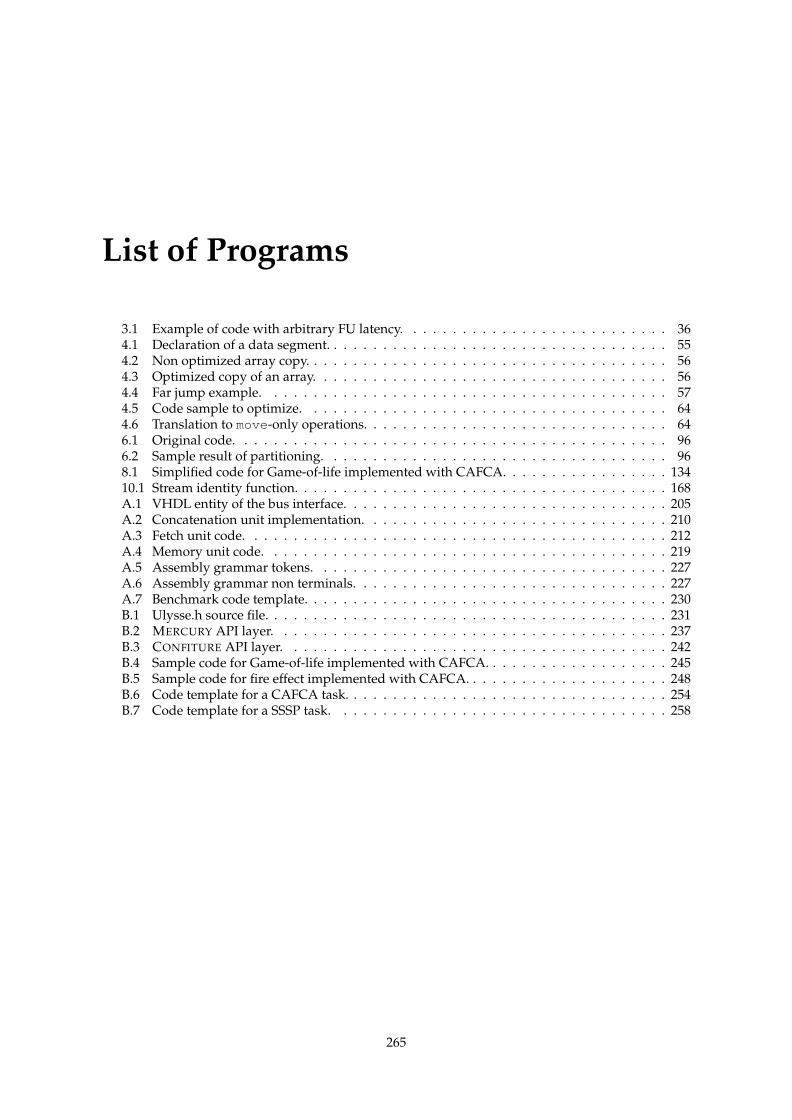
List of Programs

3.1 Example of code with arbitrary FU latency. . . . . . . . . . . . . . . . . . . . . . . . . . . 364.1 Declaration of a data segment. . . . . . . . . . . . . . . . . . . . . . . . . . . . . . . . . . . 554.2 Non optimized array copy. . . . . . . . . . . . . . . . . . . . . . . . . . . . . . . . . . . . . 564.3 Optimized copy of an array. . . . . . . . . . . . . . . . . . . . . . . . . . . . . . . . . . . . 564.4 Far jump example. . . . . . . . . . . . . . . . . . . . . . . . . . . . . . . . . . . . . . . . . 574.5 Code sample to optimize. . . . . . . . . . . . . . . . . . . . . . . . . . . . . . . . . . . . . 644.6 Translation to move-only operations. . . . . . . . . . . . . . . . . . . . . . . . . . . . . . . 646.1 Original code. . . . . . . . . . . . . . . . . . . . . . . . . . . . . . . . . . . . . . . . . . . . 966.2 Sample result of partitioning. . . . . . . . . . . . . . . . . . . . . . . . . . . . . . . . . . . 968.1 Simplified code for Game-of-life implemented with CAFCA. . . . . . . . . . . . . . . . . 13410.1 Stream identity function. . . . . . . . . . . . . . . . . . . . . . . . . . . . . . . . . . . . . . 168A.1 VHDL entity of the bus interface. . . . . . . . . . . . . . . . . . . . . . . . . . . . . . . . . 205A.2 Concatenation unit implementation. . . . . . . . . . . . . . . . . . . . . . . . . . . . . . . 210A.3 Fetch unit code. . . . . . . . . . . . . . . . . . . . . . . . . . . . . . . . . . . . . . . . . . . 212A.4 Memory unit code. . . . . . . . . . . . . . . . . . . . . . . . . . . . . . . . . . . . . . . . . 219A.5 Assembly grammar tokens. . . . . . . . . . . . . . . . . . . . . . . . . . . . . . . . . . . . 227A.6 Assembly grammar non terminals. . . . . . . . . . . . . . . . . . . . . . . . . . . . . . . . 227A.7 Benchmark code template. . . . . . . . . . . . . . . . . . . . . . . . . . . . . . . . . . . . . 230B.1 Ulysse.h source file. . . . . . . . . . . . . . . . . . . . . . . . . . . . . . . . . . . . . . . . . 231B.2 MERCURY API layer. . . . . . . . . . . . . . . . . . . . . . . . . . . . . . . . . . . . . . . . 237B.3 CONFITURE API layer. . . . . . . . . . . . . . . . . . . . . . . . . . . . . . . . . . . . . . . 242B.4 Sample code for Game-of-life implemented with CAFCA. . . . . . . . . . . . . . . . . . . 245B.5 Sample code for fire effect implemented with CAFCA. . . . . . . . . . . . . . . . . . . . . 248B.6 Code template for a CAFCA task. . . . . . . . . . . . . . . . . . . . . . . . . . . . . . . . . 254B.7 Code template for a SSSP task. . . . . . . . . . . . . . . . . . . . . . . . . . . . . . . . . . 258

265

List of Acronyms

ASIP Application Specific Instruction set Processors

CISC Complex Instruction Set Computer

CPI Clocks Per Instruction

DAG Directed Acyclic Graph

DFT Discrete Fourier Transform

DMA Direct Memory Access

EMI ElectroMagnetic Interference

EPIC Explicitely-Parallel Instruction Computing

FDCT Forward Discrete Cosine Transform

FFT Fast Fourier Transform

FPGA Field Programmable Gate Array

GPIO General Purpose Input Output

GUI Graphical User Interface

IDCT Inverse Discrete Cosine Transform

IPC Instructions Per Cycle

ILP Instruction level parallelism

IO Input Output

IR Instruction Register

JNI Java Native Interface

JTAG Joint Test Action Group

LVDS Low Voltage Differential Signalling

MPI Message Passing Interface

MPSoC Multi-processors Systems on Chip

NoC Network on Chip

OOO Out Of Order execution

PE Processing element

267

APPENDIX B. LIST OF ACRONYMS

PC Program Counter

PSL Property Specification Language

QoS Quality of Service

RF Register File

RISC Reduced Instruction Set Computer

SoC System-on-Chip

SIMD Single Instruction Multiple Data

SSA Static Single Assignment

TTA Transport Triggered Architecture

UART Universal Asynchronous Receiver Transmitter

VCC Variability Characterization Curve

VLC Variable Length Coding

VLIW Very Large Instruction Word

268

Pierre-André MudryPhD in Computer Science

Av. de Préfaully 381020 Renens, Switzerland

B pierre-andre.mudry@a3.epfl.chH +41-79-507.89.36T +41-21-634.81.89

31 years oldSwiss citizen

Education2004–2009 PhD in Computer Science, École Polytechnique Fédérale, Lausanne.

A Hardware-Software Codesign Framework for Cellular Computing1998–2004 Master in Computer Science, École Polytechnique Fédérale, Lausanne.1993-1998 Maturité cantonale, Lycée-collège de St-Guérin, Sion.

Orientation socio-économique (type E)

LanguagesFrench Native speakerGerman Basic Basic reading and writing skills. Steadily improving in speaking.English Advanced Fluent in writing and speaking. Daily use.Italian Basic Simple written and oral understanding, limited speaking.

Skills by domain

Hardware developmentArchitectures Development of DSP and MOVE processors, cellular architectures

Processors MOVE, ARM7, 8051, PIC, DSP, MicroblazeProtocols USB, I2C, SPI, PCI, 1-Wire

PCB Schematic and routing (Altium Designer and Orcad). FabricationQuality

insuranceSymbolic debugging. Code regressions and multi-level code assertion

Programming and EDASystems Linux, Windows Documents Matlab, LATEX, MS Office

Programming Java, C, C++, assembly GUI Visual Basic, C++, SwingEDA VHDL, Modelsim, Xilinx EDK and

ISE, SynplifyWeb HTML, CSS

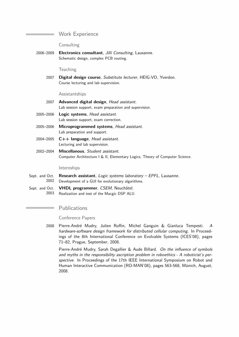
Work Experience

Consulting2006–2009 Electronics consultant, Jilli Consulting, Lausanne.

Schematic design, complex PCB routing.

Teaching2007 Digital design course, Substitute lecturer, HEIG-VD, Yverdon.

Course lecturing and lab supervision.

Assistantships2007 Advanced digital design, Head assistant.

Lab session support, exam preparation and supervision.2005–2006 Logic systems, Head assistant.

Lab session support, exam correction.2005–2006 Microprogrammed systems, Head assistant.

Lab preparation and support.2004–2005 C++ language, Head assistant.

Lecturing and lab supervision.2002–2004 Miscellanous, Student assistant.

Computer Architecture I & II, Elementary Logics, Theory of Computer Science.

InternshipsSept. and Oct.

2002Research assistant, Logic systems laboratory – EPFL, Lausanne.Development of a GUI for evolutionary algorithms.

Sept. and Oct.2003

VHDL programmer, CSEM, Neuchâtel.Realization and test of the Macgic DSP ALU.

PublicationsConference Papers

2008 Pierre-André Mudry, Julien Ruffin, Michel Ganguin & Gianluca Tempesti. Ahardware-software design framework for distributed cellular computing. In Proceed-ings of the 8th International Conference on Evolvable Systems (ICES’08), pages71–82, Prague, September, 2008.Pierre-André Mudry, Sarah Degallier & Aude Billard. On the influence of symbolsand myths in the responsibility ascription problem in roboethics - A roboticist’s per-spective. In Proceedings of the 17th IEEE International Symposium on Robot andHuman Interactive Communication (RO-MAN’08), pages 563-568, Münich, August,2008.

Andrej Gams & Pierre-André Mudry. Gaming controllers for research robots: control-ling a humanoid robot using a WIIMOTE. In Proceedings of the 17th InternationalElectrotechnical and Computer Science Conference (ERK’08), Portorož, September,2008. To appear.

2007 Pierre-André Mudry, Fabien Vannel, Gianluca Tempesti & Daniel Mange. CON-FETTI : A reconfigurable hardware platform for prototyping cellular architectures.In Proceedings of the Parallel and Distributed Processing Symposium (IPDPS’07),pages 1–8, Long Island, March, 2007.

2006 Pierre-André Mudry, Guillaume Zufferey & Gianluca Tempesti. A dynamically con-strained genetic algorithm for hardware-software partitioning. In Proceedings of the8th annual Conference on Genetic and Evolutionary Computation (GECCO’06), pages769–776, Seattle, July, 2006.Gianluca Tempesti, Daniel Mange, Pierre-André Mudry, Joël Rossier & André Stauf-fer. Self-replication for reliability: bio-inspired hardware and the embryonics project.In Proceedings of the 3rd Conference on Computing frontiers, pages 199–206, Ischia,2006.Gianluca Tempesti, Pierre-André Mudry & Guillaume Zufferey. Hardware/softwarecoevolution of genome programs and cellular processors. In Proceedings of the 1stNASA/ESA Conference on Adaptive Hardware and Systems (AHS’06), pages 129–136, Istanbul, June, 2006.Pierre-André Mudry, Guillaume Zufferey & Gianluca Tempesti. A hybrid genetic algo-rithm for constrained hardware-software partitioning. In Proceedings of the 2006 IEEEWorkshop on Design and Diagnostics of Electronic Circuits and Systems (DDECS’06),pages 3–8, Prague, April, 2006.Joël Rossier, Yann Thoma, Pierre-André Mudry & Gianluca Tempesti. MOVE pro-cessors that self-replicate and differentiate. In Proceedings of the 2nd InternationalWorkshop on Biologically Inspired Approaches to Advanced Information Technology(BioADIT’06), pages 160–175, Osaka, January, 2006.

2005 Gianluca Tempesti, Pierre-André Mudry & Ralph Hoffmann. A MOVE processor forbio-inspired systems. In Proceedings of the NASA/DoD Conference on EvolvableHardware (EH’2005), pages 262–271, Washington, June, 2005.

Journal papers2007 Gianluca Tempesti, Daniel Mange, Pierre-André Mudry, Joël Rossier & André Stauf-

fer. Self-replicating hardware for reliability: The embryonics project. In ACM Journalon Emerging Technologies in Computing Systems (JETC), volume 3, number 2, 2007.