A H -A A -I SYSTEMS - McGill Universitydigitool.library.mcgill.ca/thesisfile95154.pdf · et les...
102
Mathieu Paul Constantin PELLISSIER, 2010, All rights reserved OPTIMIZATION VIA CFD OF AIRCRAFT HOT-AIR ANTI-ICING SYSTEMS MATHIEU PAUL CONSTANTIN PELLISSIER Computational Fluid Dynamics Laboratory, Department of Mechanical Engineering, McGill University, Montréal, Québec, Canada June 2010 A thesis submitted to McGill University in partial fulfillment of the requirements of the degree of Master of Engineering
Transcript of A H -A A -I SYSTEMS - McGill Universitydigitool.library.mcgill.ca/thesisfile95154.pdf · et les...

Mathieu Paul Constantin PELLISSIER, 2010, All rights reserved
OPTIMIZATION VIA CFD
OF
AIRCRAFT HOT-AIR ANTI-ICING SYSTEMS
MATHIEU PAUL CONSTANTIN PELLISSIER
Computational Fluid Dynamics Laboratory, Department of Mechanical Engineering,
McGill University, Montréal, Québec, Canada
June 2010
A thesis submitted to McGill University in partial fulfillment of the requirements of
the degree of Master of Engineering

ii
ACKNOWLEDGEMENTS
I would like to especially thank my supervisor Professor Wagdi Habashi for having
made this privileged experience possible and for his precious advice and guidance all
along this Master’s research project.
I would like to gratefully acknowledge the fact that this project was funded by the
NSERC - J. Armand Bombardier Industrial Research Chair for Multidisciplinary CFD.
I would also like to address a special thanks to my lab-mates at the CFD Lab whose
support and contributions were particularly appreciated. Thank you very much to
Mostafa Najafiyazdi, Dr. Marco Fossati, Vladislav Lappo, Shezad Nilamdeen, Amir
Borna, and Dr. Rooh-Ul-Amin Khurram.
I would like to gratefully thank Dr. Alberto Pueyo and Corentin Brette from
Bombardier Aerospace Advanced Aerodynamics Aero-Icing Group for their advice,
time and consideration.
I would also like to mention the highly appreciated availability and help of Yves
Simard, the CFD Lab’s System Administrator, the NTI (Newmerical Technologies
International) team, Dr. Guido Baruzzi, Martin Aubé, HongZhi Wang, Karim Moumen,
Patrick Lagacé, Cristhian Aliaga, Thomas Reid and Bruno Cassagne, and from the
CFD Lab Associate Professor, Dr. Siva Nadarajah.
Last, but not least, I would like to gratefully thank my fiancée Maude for her
unconditional support through this entire project.

iii
ABSTRACT
In-flight icing is a major concern in aircraft safety and a non-negligible source of
incidents and accidents, and is still a serious hazard today. It remains consequently a
design and certification challenge for aircraft manufacturers. The aerodynamic
performance of an aircraft can indeed degrade rapidly when flying in icing conditions,
leading to incidents or accidents. In-flight icing occurs when an aircraft passes
through clouds containing supercooled water droplets at or below freezing
temperature. Droplets impinge on its exposed surfaces and freeze, causing
roughness and shape changes that increase drag, decrease lift and reduce the stall
angle of attack, eventually inducing flow separation and stall. This hazardous ice
accretion is prevented by the use of dedicated anti-icing systems, among which hot-
air-types are the most common for turbofan aircraft.
This work presents a methodology for the optimization of such aircraft hot-air-type
anti-icing systems, known as Piccolo tubes. Having identified through 3D
Computational Fluid Dynamics (CFD) the most critical in-flight icing conditions, as
well as determined thermal power constraints, the objective is to optimize the heat
distribution in such a way to minimize power requirements, while meeting or
exceeding all safety regulation requirements. To accomplish this, an optimization
method combining 3D CFD, Reduced-Order Models (ROM) and Genetic Algorithms
(GA) is constructed to determine the optimal configuration of the Piccolo tube (angles
of jets, spacing between holes, and position from leading edge). The methodology
successfully results in increasingly optimal configurations from three up to five design
variables.

iv
RESUME
Le givrage en vol constitue encore et toujours un souci majeur de sûreté en aviation
et demeure une source non négligeable d’incidents et d’accidents. Ainsi, le givrage en
vol reste un défi de taille en termes de conception et de certification pour les
constructeurs aéronautiques. Les performances aérodynamiques d’un avion peuvent
en effet se dégrader rapidement quand il vole en conditions givrantes, et ainsi
engendrer des incidents ou même des accidents. Le givrage en vol a lieu quand un
avion traverse des nuages contenant des gouttelettes d’eau surfondues à des
températures inférieures ou égales au point de congélation. Les gouttelettes
impactent sur les zones exposées et gèlent, ce qui augmente la rugosité, provoquant
une augmentation de la traînée, une diminution de la portance et de l’angle de
décrochage, et induisant éventuellement la séparation de l’écoulement et le
décrochage. L’accrétion de glace est empêchée par l’utilisation de systèmes dédiés
d’antigivrage, parmi lesquels les systèmes à air chaud sont les plus utilisés par les
avions de ligne.
Cet ouvrage présente une méthodologie en vue de l’optimisation de tels systèmes
d’antigivrage à air chaud appelés tubes Piccolo. Ayant identifié les conditions de
givrage en vol les plus sévères à l’aide de la CFD (Computational Fluid Dynamics, ou
simulation numérique en dynamique des fluides) tridimensionnelle ainsi que les
contraintes de puissance thermique liées au système de dégivrage, l’objectif est
d’optimiser la distribution de chaleur de façon à minimiser la puissance thermique
requise, tout en satisfaisant aux réglementations de sûreté en vol. Dans ce but, une
méthode d’optimisation combinant la CFD 3D, la Modélisation d’Ordre Réduit (MOR)
et les Algorithmes Génétiques (AG), est développée afin de déterminer la
configuration optimale du tube Piccolo (en termes d’angles de jets, de distance entre
les jets et de distance au bord d’attaque). Cette méthodologie mène à des
configurations d’optimalité croissante de trois à cinq variables.

v
TABLE OF CONTENTS
ACKNOWLEDGEMENTS ................................................................................ II
ABSTRACT ............................................................................................. III
RESUME ................................................................................................IV
TABLE OF CONTENTS ................................................................................. V
NOMENCLATURE ...................................................................................... VII
LIST OF FIGURES ...................................................................................... X
LIST OF TABLES ..................................................................................... XIII
1. INTRODUCTION .................................................................................. 1
1.1 In-Flight Icing ............................................................................... 1
1.2 In-Flight Icing Protection: Anti-Icing/De-Icing ................................... 3
1.3 Experimental and Numerical In-Flight Icing ...................................... 4
1.4 Objective of the Current Work ......................................................... 5
2. STATE OF THE ART .............................................................................. 6
2.1 Physical Models ............................................................................. 6
2.2 Aircraft In-Flight Anti-Icing Systems ................................................ 6
2.3 Impinging Jet Flow ........................................................................ 7
2.4 Anti-Icing Systems Optimization Methodology ................................... 8
3. OPTIMIZATION METHODOLOGY .............................................................. 10
3.1 Parameterization ......................................................................... 10
3.1.1 Geometry of the System ......................................................................... 10
3.1.2 Parameterization of the Problem .............................................................. 11
3.2 Optimization Methodology ............................................................ 12
3.2.1 Overview .............................................................................................. 12
3.2.2 Genetic Algorithms ................................................................................. 14
vi
3.2.3 Objective Function ................................................................................. 16
3.2.4 Proper Orthogonal Decomposition ............................................................ 18
3.3 Numerical Models ........................................................................ 21
3.3.1 External Flow ........................................................................................ 21
3.3.2 Internal Flow ......................................................................................... 22
3.3.3 From 3D Internal Flow Simulation to 3D Internal Flow Correlation ................ 23
3.3.4 Water Runback ...................................................................................... 26
3.3.5 Validation Results .................................................................................. 33
4. APPLYING THE OPTIMIZATION METHODOLOGY ............................................ 36
4.1 Genetic Algorithm’s Convergence .................................................. 36
4.2 3-Design-Variable Configurations .................................................. 40
4.3 4-Design-Variable Configurations .................................................. 41
4.4 5-Design-Variable Configuration .................................................... 42
4.5 Results Summary ........................................................................ 43
CONCLUSION AND FUTURE WORK ................................................................ 47
REFERENCES ......................................................................................... 48
APPENDIX A .......................................................................................... 54
A. SENSITIVITY ANALYSIS OF THE IMPACT OF WALL TEMPERATURE ...................... 54
APPENDIX B .......................................................................................... 63
B. 3D-CFD-BASED HEAT TRANSFER COEFFICIENT CORRELATION ....................... 63
APPENDIX C.......................................................................................... 74
C. APPROXIMATION OF WATER RUNBACK SOLUTION USING POD ........................ 74
APPENDIX D ......................................................................................... 82
D. DIRECT OPTIMIZATION VERSUS SEQUENTIAL OPTIMIZATION .......................... 82

vii
NOMENCLATURE
Symbols
A, Γ Energy equation influence matrix [J/s/K]
[b], [b°], [b*] Energy equation Right Hand Side vector [J/s]
c Distance between adjacent jets [m]
cp Specific heat capacity [J/kg/K]
d Piccolo tube jet nozzle diameter [m]
dr Radius increment [m]
dZW Spanwise width of local cell [m]
D Piccolo tube diameter [m]
e Airfoil skin thickness [m]
f Freezing fraction []
frec Recovery factor []
GA Genetic Algorithm
hc Local heat transfer coefficient [W/m²/K]
hf Local water film height [m]
Hr Relative humidity []
k Thermal conductivity of the fluid [W/m/K]
K Continuity equation influence matrix [kg/s/m]
Lfus Latent heat of fusion [J/m3]
Lvap Latent heat of vaporization [J/m3]
LWC Liquid Water Content [kg/m3]
M Mach number []
m Mass flow rate [kg/s]
m Mass flux [kg/s/m²]
nm Number of modes
ns Number of snapshots
Nur Local Nusselt number based on Piccolo hole diameter [], cNu h d k
Nu Mean Nusselt number based on Piccolo hole diameter [], cNu h d k
ObjFct Objective function []
p Penalty factor []
P, Ps Local static pressure [Pa]
Pvap Saturation vapor pressure [Pa]
POD Proper Orthogonal Decomposition

viii
Pr Prandtl number [], Pr Cp k
Q Thermal power [J/s]
Q Heat flux [J/s/m2]
r, R Radial distance from Piccolo jet axis [m]
[R] Energy equation residual vector [J/s]
Re Jet Reynolds number [], Re 4 jetm d
ROM Reduced Order Model
s Curvilinear coordinate [m]
S Surface area of local cell [m2]
T , T Local and reduced local temperature [K], 273.15T T
[T] Temperature vector [K]
Uj POD snapshot solution vector [-]
Û POD target solution vector [-]
Ud Droplet free stream velocity [m/s]
fU Water film mean velocity [m/s]
U, V Velocity [m/s]
XPic, YPic Local Cartesian coordinates of the Piccolo tube axis [m]
zn Normal distance from Piccolo hole to internal surface skin [m]
α Relaxation factor []
αij POD snapshot coefficient []
ˆi POD target coefficient []
β Water droplets collection efficiency
[Δhf] Film height delta vector [m]
Δs Length of local cell [m]
[ΔT] Temperature delta vector [K]
ε Skin emissivity []
θ Jet orientation angle [°]
λ Thermal conductivity of the metal skin [W/m/K]
μ Dynamic viscosity [Pa.s]
ρ Density [kg/m3]
τW Wall shear stress [Pa]
σ Boltzmann constant [σ =5.670×10⁻⁸ W/m2/K4]
Φi POD eigenfunction [-]

ix
Subscripts
adiab Adiabatic
anti-ice Anti-icing
cond Conduction
conv Convection
d Droplet
evap, vap Evaporation
exhaust Piccolo exhaust
ext External flow
f Water film
fus Fusion
ice Ice
ideal Ideal target
in, IN Coming in the control volume
int Internal flow
jet Piccolo jet
loss Losses within Piccolo tube system
mean Mean
out, OUT Coming out of the control volume
Pic Piccolo tube
rad Radiation
rb Water runback
ref Reference value
tot Total
w Water
W Wall
β Droplet impingement
∞ External flow free-stream value
Superscripts
POD Derived from POD solution
total Over the entire leading edge
upper Over the upper surface of the leading edge
x
LIST OF FIGURES
Figure 1-1: Aircraft components affected by in-flight icing, and effect. .................................. 1
Figure 1-2: Rime ice (left) and glaze ice (right) ................................................................. 2
Figure 1-3: Additional non-negligible side effects of in-flight icing ........................................ 2
Figure 1-4: Aerodynamic effects of in-flight icing ............................................................... 3
Figure 3-1: 3D generic constant chord swept wing. .......................................................... 10
Figure 3-2: Piccolo tube section on the wing slat in smooth configuration. ........................... 10
Figure 3-3: Piccolo tube geometric configuration. ............................................................. 11
Figure 3-4: Geometric parameters. ................................................................................ 12
Figure 3-5: Optimization methodology diagram. .............................................................. 13
Figure 3-6: Genetic algorithms procedure. ...................................................................... 14
Figure 3-7: Illustration of the concepts of local POD and local Kriging in 2D. ....................... 21
Figure 3-8: 3D flow around swept wing (left) and corresponding droplet impingement (right).
........................................................................................................................... 22
Figure 3-9: 3D internal flow inside Piccolo anti-icing system. ............................................. 23
Figure 3-10: Internal heat transfer coefficient distribution from CFD and correlation............. 24
Figure 3-11: Mass and energy balance over a control volume. ........................................... 26
Figure 3-12: Water film breaking into rivulets. ................................................................. 31
Figure 3-13: Example of water film solution. ................................................................... 32
Figure 3-14: Experimental and numerical icing test results. ............................................... 34
Figure 3-15: Sketch of a slat hot-air anti-icing system section. .......................................... 35
Figure 4-1: Genetic algorithm’s convergence. .................................................................. 36
Figure 4-2: 2D optimization example. ............................................................................. 37
Figure 4-3: Initial population uniformly spread using Lp-τ. ................................................ 37
Figure 4-4: Partial GA convergence. ............................................................................... 38
Figure 4-5: Final GA convergence. ................................................................................. 38
Figure 4-6: Optimal design configuration versus slightly off-design configurations. ............... 39
Figure 4-7: Initial generic configuration and corresponding water runback. ......................... 40
Figure 4-8: First 3-design-variable optimal configuration and corresponding water runback. . 41
Figure 4-9: Second 3-design-variable optimal configuration and corresponding water runback.
........................................................................................................................... 41
Figure 4-10: First 4-design-variable optimal configuration and corresponding water runback. 42
Figure 4-11: Second 4-design-variable optimal configuration and corresponding water runback.
........................................................................................................................... 42
Figure 4-12: 5-design-variable optimal configuration and corresponding water runback. ....... 43
Figure 4-13: Optimal configuration obtained without POD and corresponding water runback. 46
Figure A-1. Imposed wall temperature boundary conditions. ............................................. 54
Figure A-2. Wall pressure distribution along the skin. ....................................................... 55

xi
Figure A-3. Wall shear stress distribution along the skin. .................................................. 55
Figure A-4. Convective heat flux distribution along the skin. .............................................. 56
Figure A-5. Heat transfer coefficient distribution along the skin. ......................................... 56
Figure A-6. Local liquid water content distribution along the skin. ...................................... 57
Figure A-7. Collection efficiency distribution along the skin. ............................................... 58
Figure A-8. Impingement mass flux distribution along the skin. ......................................... 58
Figure A-9. Temperature boundary condition on the inner skin wall. ................................... 59
Figure A-10. Heat transfer coefficient distribution on the inner skin wall for cases 1 & 3. ....... 60
Figure A-11. Relative error distribution on the inner skin wall for cases 1 & 3. ..................... 60
Figure A-12. Heat transfer coefficient distribution on the inner skin wall for cases 1 & 2. ....... 61
Figure A-13. Relative error distribution on the inner skin wall for cases 2 & 3. ..................... 61
Figure A-14. Heat transfer coefficient distribution on the inner skin wall for cases 2 & 3. ....... 62
Figure A-15. Relative error distribution on the inner skin wall for cases 1 & 2. ..................... 62
Figure B-1. Heat transfer coefficient distributions from original correlation vs. CFD. ............. 64
Figure B-2. Water film thickness distributions with HTC from original correlation vs. CFD. ..... 65
Figure B-3. Original correlation variations with normal distance and radial distance. ............. 65
Figure B-4. New correlation variations with normal distance and radial distance. .................. 65
Figure B-5. HTC distributions from new correlation vs. CFD, case # 1. ................................ 66
Figure B-6. HTC distributions from new correlation vs. CFD, case # 1 (close-up).................. 66
Figure B-7. HTC distributions from new correlation vs. CFD, case # 2. ................................ 67
Figure B-8. HTC distributions from new correlation vs. CFD, case # 2 (close-up).................. 67
Figure B-9. HTC distributions from new correlation vs. CFD, case # 3. ................................ 68
Figure B-10. HTC distributions from new correlation vs. CFD, case # 3 (close-up). ............... 68
Figure B-11. HTC distributions from new correlation vs. CFD, case # 4. .............................. 69
Figure B-12. HTC distributions from new correlation vs. CFD, case # 4 (close-up). ............... 69
Figure B-13. HTC distributions from new correlation vs. CFD, case # 5. .............................. 70
Figure B-14. HTC distributions from new correlation vs. CFD, case # 5 (close-up). ............... 70
Figure B-15. HTC distributions from new correlation vs. CFD, case # 6. .............................. 71
Figure B-16. HTC distributions from new correlation vs. CFD, case # 6 (close-up). ............... 71
Figure B-17. HTC distributions from new correlation vs. CFD, case # 7. .............................. 72
Figure B-18. HTC distributions from new correlation vs. CFD, case # 7 (close-up). ............... 72
Figure B-19. HTC distributions from new correlation vs. CFD, case # 8. .............................. 73
Figure B-20. HTC distributions from new correlation vs. CFD, case # 8 (close-up). ............... 73
Figure C-1. Original and POD water runback mass flow distributions for 3 design variables. .. 75
Figure C-2. Original and POD wall temperature distributions for 3 design variables. .............. 75
Figure C-3. Original and POD water runback mass flow distributions for 3 design variables. .. 76
Figure C-4. Original and POD wall temperature distributions for 3 design variables. .............. 76
Figure C-5. Original and POD water runback mass flow distributions for 4 design variables. .. 77
Figure C-6. Original and POD wall temperature distributions for 4 design variables. .............. 77

xii
Figure C-7. Original and POD water runback mass flow distributions for 4 design variables. .. 78
Figure C-8. Original and POD wall temperature distributions for 4 design variables. .............. 78
Figure C-9. Original and POD water runback mass flow distributions for 5 design variables. .. 79
Figure C-10. Original and POD wall temperature distributions for 5 design variables. ............ 79
Figure C-11. Original and POD water runback mass flow distributions for 5 design variables. . 80
Figure C-12. Original and POD wall temperature distributions for 5 design variables. ............ 80
Figure D-1. 2D optimization example via direct optimization. ............................................. 82
Figure D-2. Direct optimization from initial to final GA generation. ..................................... 83
Figure D-3. 2D optimization example via sequential optimization: first step......................... 84
Figure D-4. Sequential optimization step 1: from initial to final GA generation. .................... 85
Figure D-5. Sequential optimization step 2: from initial to final GA generation. .................... 86
Figure D-6. Sequential optimization step 3: from initial to final GA generation. .................... 87
Figure D-7. Sequential optimization step 4: from initial to final GA generation. .................... 88

xiii
LIST OF TABLES
Table 1: Mass balance terms ......................................................................................... 29
Table 2: Energy balance terms ...................................................................................... 29
Table 3: Icing experimental test case parameters. ........................................................... 33
Table 4. Summary of the different optimal configurations compared to initial generic design. 43
Table 5. Consecutive optimal configurations compared to initial generic design. ................... 44
Table 6. Optimal configuration obtained without POD. ...................................................... 45
1
1. INTRODUCTION
1.1 In-Flight Icing
In-flight icing is a major concern in aircraft safety, a non-negligible source of
accidents and is still a serious hazard today [1-3]. As a consequence, it remains a
design and certification challenge for the aircraft manufacturers.
Indeed, the aerodynamic performance of an unprotected aircraft flying in icing
conditions can degrade rapidly and if not treated appropriately, lead to incidents and
accidents. In-flight icing generally occurs at or below the freezing point when an
aircraft passes through clouds containing supercooled droplets [4-9] (unstable
physical state where droplets remain liquid even far below freezing point). Also,
freezing rain can occur at the interface between warm and cold fronts (in this case,
the droplets are usually of bigger size and referred to as “Supercooled Large
Droplets” or SLD).
Aerodynamic surfaces Anti-icing or de-icing
system
Impact on aerodynamic
performance and control
Engine inlets
Anti-icing or de-icing
system
Impact on engine
performance
Wind shield Electro-thermal anti-
icing system
Impact on visibility
Radome, antennas, probes Electro-thermal anti-icing
system
Impact on communication
Figure 1-1: Aircraft components affected by in-flight icing, and effect.
Supercooled droplets impinging on the aircraft’ exposed surfaces (cf. Figure 1-1,
adapted from [10]) will either freeze upon impact to form rime ice, or run back on
the surface and freeze further downstream to form glaze ice. In rime-ice conditions
or “dry regime” (usually for air temperatures below -20°C) the ice will accrete in a
dense opaque streamlined shape. In glaze-ice conditions or “wet regime” (usually for
air temperatures between 0°C and -20°C) the ice will accrete in transparent irregular
horn-like shapes (cf. Figure 1-2). Mixed-ice conditions can also be encountered. The
severity of ice accretion, in terms of quantity and location, is affected by:
The flight configuration:

2
- Free-stream velocity
- Angle of Attack (AoA)
- Altitude
- High-lift systems configuration
- Flight phase
The icing conditions:
- Ambient air temperature
- Liquid Water Content (LWC)
- Droplet size distribution
These parameters directly impact the droplet collection efficiency and the ice
accretion is then highly dependent on the exposure time and the efficiency of the
anti-icing system.
Figure 1-2: Rime ice (left) and glaze ice (right)
Beside the risks of decreasing pilots’ visibility and putting in jeopardy the efficiency of
the aircraft radar, communication antennas and probes (cf. Figure 1-3), in-flight icing
can considerably affect the aerodynamic as well as control and stability performances
of the aircraft.
Figure 1-3: Additional non-negligible side effects of in-flight icing
Droplets impinge on the exposed surfaces of the aircraft and freeze, increasing
surface roughness and inducing early boundary-layer transition to turbulent flow. Ice
accretion also leads rapidly to increased drag, decreased lift (cf. Figure 1-4), with a

3
corresponding increase in stall speed and decrease in stall angle which constitute
propitious conditions for flow separation and stall even at sometimes significantly
lower angles of attack [5, 7, 9, 11], especially in the maneuver, holding, take-off and
landing phases. It will also modify the pressure distribution and the load dispatch,
induce vibrations and decrease the aircraft’s maneuverability. In-flight icing is also an
issue for engines and propellers, degrading performances, blocking inlets, and
possibly damaging in case of ice ingestion.
Figure 1-4: Aerodynamic effects of in-flight icing
1.2 In-Flight Icing Protection: Anti-Icing/De-Icing
To avoid such events, aircraft are equipped with systems to prevent ice accretion on
the exposed critical aerodynamic and control surfaces during flight. These anti-icing
systems must comply with flight safety regulations outlined by national certification
authorities such as the FAA [5-6, 12] (Federal Aviation Administration), the EASA
[13] (European Aviation Safety Agency) and Transport Canada [14], or other
governmental entities [7-9].
As opposed to ground icing, which can be visually checked and taken care of on the
runway, in-flight icing requires rigorous procedures and systems to address flight
safety regulations outlined by national certification authorities. Such systems include
ice detection systems coupled to ice protection systems (de-icing or anti-icing
systems), usually located at the leading edge of the exposed surfaces. De-icing
systems are reactive and commonly consist in mechanically deformable membranes
or electro-impulse devices. Such systems are used periodically to remove already
accreted ice. Anti-icing systems, such as hot-bleed-air circulation systems or electro-
thermal devices, are preemptive and designed to prevent ice accretion by
evaporating the impinging droplets.
One of the most widely used anti-icing devices for wings, stabilizer and engine
nacelles of commercial and corporate turbofan engine aircraft is a high-temperature

4
bleed-air anti-icing system, commonly called Piccolo tube. This system circulates hot-
air, collected from the engine’s first compressor, to the areas to be protected.
1.3 Experimental and Numerical In-Flight Icing
The physics of in-flight icing have been greatly investigated and are increasingly
understood, but not yet totally elucidated. Numerical models have been developed to
compute ice accretion, evaluate the consequent performance degradation, study and
design anti-icing systems and evaluate their efficiency and performance throughout
the in-flight icing envelop. In-flight icing software were usually focused on the
external aspect, meaning the external flow, droplet impingement and computing the
ice accretion, all this mostly in 2D. Some additional features like coupling with bleed-
air systems internal flow or with electro-thermal anti-icing were developed to further
study the anti-icing aspect itself. The new generation of software, like FENSAP-ICE,
has the capability to handle 3D complex geometries in a coupled way with all
external flow, droplet impingement, internal flow, heat conduction and ice accretion
thermodynamics, in the case of steady or unsteady ice accretion.
On the one hand, flight-testing in natural icing conditions is expensive, and difficult
to run since it is dangerous and not all conditions outlined in the FAA’s FAR (Federal
Airworthiness Regulations) Part 25 Appendix C [12] or the EASA’s CS (Certification
Specifications) Part 25 Appendix C [13] can be reproduced. On the other hand, icing-
wind-tunnel-testing is costly and somewhat limiting. Both approaches are suitable for
analyzing a system but can hardly be used as a design platform. Therefore, it is
logical to benefit from CFD to model and optimize anti-icing systems, before they are
built and tested.
Nevertheless, fully-coupled 3D simulations including 3D external flow, corresponding
water impingement and ice accretion, 3D conduction through the skin and 3D
internal flow coupled using Conjugate Heat Transfer (CHT), are quite demanding in
terms of computing resources. As a result, exploring the design space to come up
with an optimal design, which would require a large number of CFD simulations,
would not be cost-effective in an industrial framework.
As the number of design variables is relatively high and their combination leads to a
large variety of configurations, the design space is wide and possesses several local
extrema. In such conditions, classic gradient-based optimization methods are
inefficient and most often get stuck in local extrema.
In order to study the sensitivity of anti-icing power to geometric parameters of the
Piccolo, a substantial number of CFD simulations of the 3D external and internal

5
flows need to be conducted. The size of meshes being relatively large, this demands
quite important computational resources.
1.4 Objective of the Current Work
It is important to consider that safety has a significant cost. Indeed the amount of air
bled from the engine for ice protection, along with conditioning and cabin
pressurization can represent 5% to 10% of the core engine mass flow [15], half of
which is for anti-icing purpose alone [16]. Additionally, bleed-air collection induces
engine performance penalties such as increase of specific fuel consumption, power
loss and increase in turbine gas temperature [15-16]. The high bypass ratios and the
ever-smaller core engine sizes of the modern turbofan engines make it crucial to
maximize anti-icing system efficiency in order to minimize the amount of necessary
bleed air.
The present work’s motivation is thus to develop a Piccolo tube optimization
methodology, with the idea of firstly uncoupling the problem to limit its size, secondly
using a Reduced-Order Model (ROM), such as Proper Orthogonal Decomposition
(POD), to limit the number of necessary computations, and thirdly applying an
evolutionary optimization approach, such as Genetic Algorithms (GA), to efficiently
search the wide multidimensional design space. This approach focuses, in the context
of this Master’s research project, on single objective optimization based on geometric
parameters. The associated models are 3D CFD-based and include solving for water
runback.
This work will first introduce the state of the art of bleed-air anti-icing systems study,
then present the optimization methodology and the different models, next provide
test case results, and finally draw conclusions and outline some recommendations for
future work.
6
2. STATE OF THE ART
2.1 Physical Models
In-flight icing and anti-icing topics are widely addressed in the literature. The
physical models dealing with ice accretion and water film runback phenomena are
usually based on a Messinger-type control-volume-based finite difference scheme
[17-24] and possibly including the anti-icing aspect [25-35]. These icing simulations
are run using commercial, in-house or research icing codes like LEWICE [10, 36],
ICECREMO [23, 26], ANTICE [37] or CANICE [31-34, 38-39] which rely on CFD
computations using CFD commercial or in-house codes to get the external flow
and/or water droplet impingement solutions. Fully integrated CFD/Icing packages
also exist, such as FENSAP-ICE [40-46], which even provides a Conjugate Heat
Transfer (CHT) framework to execute fully coupled1 in-flight icing computations to
simulate anti-icing systems.
2.2 Aircraft In-Flight Anti-Icing Systems
Some of the anti-icing studies focus on electro-thermal anti-icing systems [26-30,
32-33, 37, 47-48] which are usually easier to implement since for all practical
purposes the problem can be reduced to 2D and the anti-icing heat flux distribution is
directly applied as a wall boundary condition.
In this work, the attention is focused on the study of hot-bleed-air anti-icing systems
which are widely covered in the literature [15, 25, 31, 34, 36, 38-39, 42, 45, 49-65].
Current methods include 2D icing CFD-based uncoupled simulations in “wet air”2
conditions which rely on heat transfer coefficient correlations to represent the
internal flow [25, 31, 34], 2D uncoupled CFD simulations of the 2D internal flow [39]
and 2D icing CFD-based coupled simulations, using CFD to compute the internal flow,
in “dry air” [54] and “wet air” [38] conditions.
2.5D3 icing CFD-based coupled simulations in “wet air” conditions, using CFD to
compute the internal flow, is mentioned in [36].
1 The term “coupled” refers to the fact that external flow and internal flow solutions are computed in a coupled manner, usually
through CHT, with or without considering the conduction within the skin.
2 As opposed to “dry air”, “wet air” means that the LWC is non-zero and thus implies solving for droplet impingement, water runback
and ice accretion. 3 2.5D stands for solving external and internal flows in 3D and computing water runback and ice accretion in a two-dimensional
manner.

7
3D icing CFD-based coupled simulations, using CFD to compute the internal flow,
were also covered in “dry air” [45, 50, 53-55] and “wet air” conditions [42].
Most of these studies compared their results against experimental icing tunnel test
results or against other computational results obtained with different codes.
Also, experimental [57, 61, 63] and computational [15, 58, 60, 64] investigations
and parametric studies of hot-air anti-icing systems were carried out to evaluate the
efficiency and performance of such systems, investigate their sensitivity to in-flight
icing conditions and Piccolo tube geometric and thermodynamic parameters, and
examine their behavior to off-design conditions.
2.3 Impinging Jet Flow
The study of heat transfer from an impinging jet onto a surface is also a well-
addressed topic. The local Nusselt number is recovered either from heat/mass
transfer analogy using the sublimation of a volatile chemical like naphthalene at the
wall, or from the temperature distribution when imposing a constant and uniform
heat flux via a thin metallic foil covering the surface. The main objective of such
studies is usually to investigate experimentally and/or numerically the impact of
certain parameters such as the jet Reynolds number, the normal distance from hole
to surface, the jet diameter and the radial distance from the jet stagnation point, on
the heat transfer to the wall, in order to elaborate a correlation for the average
Nusselt number.
For this purpose, experimental studies of a single impinging jet on a flat plate are
done [66-71]. Also, parametric investigations about staggered impinging jet arrays
on a flat plate were addressed experimentally and/or numerically [72-74], including
the effect of the jet-to-jet spacing on the Nusselt number [72, 74].
In order to get more specific to the Piccolo tube anti-icing system geometry, 3D
numerical studies of the flow and heat transfer of an hot-air impinging jet array on a
concave surface were proposed [52, 75].
Moreover, experimental and numerical studies were engaged directly on hot-air anti-
icing systems to obtain Nusselt number correlations. Brown et al. [49] ran
experimental investigations on a nacelle inlet hot-air anti-icing system model, a
three-row staggered jet array Piccolo tube, and proposed an average Nusselt number
correlation independent of the normal distance from hole to surface.
Planquart et al. [59] presented an experimental and numerical study on a wing slat
three-row staggered jet array Piccolo tube, using infrared thermography combined
with the heating foil method to recover the thermal exchange coefficient distribution.

8
The experimental data is used to obtain a Nusselt number correlation and to validate
the corresponding numerical simulations.
Wright [65] presented a review of Nusselt number correlations for three-row
staggered jet Piccolo tube application. The aim of the study was to do an evaluation
of the jet impingement heat transfer correlations by integrating them to anti-icing
numerical simulations and validating against experimental data in “wet air”
conditions.
2.4 Anti-Icing Systems Optimization Methodology
Up to this point, the optimization as such of anti-icing systems was not addressed
and is not widely represented in the literature; quite the contrary.
Wang et al. [48] proposed a thermo-fluid optimization methodology to improve the
de-icing strategy thermal effectiveness of an electrically-heated intake scoop of a
helicopter engine cooling-bay inlet. The optimization method involved the Latin
Hypercube Design of Experiments (DOE) method, the Boender-Timmer-Rinnooy-Kan
(BTRK) clustering algorithm coupled with an adaptive-response-surface-based
reduced-order model method. The methodology was able to handle up to four
geometric parameters and one thermodynamic parameter as design variables.
Concerning hot-bleed-air anti-icing systems, there are two particularly relevant
articles of great insight in terms of optimization methods.
Santos et al. [76] performed a sensitivity analysis on a 6-parameter internal flow
correlation that was coupled with external flow, droplet impingement and ice
accretion 2D solvers. The sensitivity analysis methodology was performed to reveal
the most significant geometrical and operational parameters of the hot-bleed-air
anti-icing system in order to provide guidelines for parametric optimization. This
methodology, which does not strictly speaking constitute an optimization procedure,
relies on a Sobol design of experiments procedure and a response-surface-based
reduced-order model method. It was able to handle four geometric parameters and
two thermodynamic parameters as design variables.
Last but not least, Saeed and Paraschivoiu [77] used a Micro-Genetic-Algorithm
optimization code to determine the optimum Piccolo tube configuration for a given
range of flight and icing conditions. The methodology relied on an internal flow 2D
correlation coupled with the 2D icing code CANICE and managed two independent
geometric parameters and one thermodynamic parameter as design variables. The
problem is set like a multi-objective optimization problem with two icing parameters
and three flight parameters defined within a chosen in-flight icing envelop. Their

9
preliminary results suggested that the genetic-algorithm-based optimization had a
great application potential for the design of hot-air anti-icing systems.
These references were of great interest and inspiration for the elaboration of the
optimization methodology presented in this work.
The present work’s optimization methodology is pushed further by incorporating the
3D external flow CFD solution and an internal flow 3D CFD-based correlation to a
Messinger water film model, with the possibility to integrate higher fidelity solutions,
and by combining “classic” (as opposed to micro) genetic algorithms and POD-based
reduced-order model and managing up to five independent geometric parameters as
design variables.
10
3. OPTIMIZATION METHODOLOGY
3.1 Parameterization
3.1.1 Geometry of the System
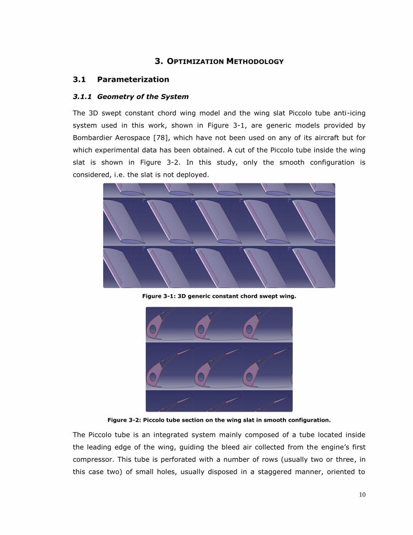
The 3D swept constant chord wing model and the wing slat Piccolo tube anti-icing
system used in this work, shown in Figure 3-1, are generic models provided by
Bombardier Aerospace [78], which have not been used on any of its aircraft but for
which experimental data has been obtained. A cut of the Piccolo tube inside the wing
slat is shown in Figure 3-2. In this study, only the smooth configuration is
considered, i.e. the slat is not deployed.
Figure 3-1: 3D generic constant chord swept wing.
Figure 3-2: Piccolo tube section on the wing slat in smooth configuration.
The Piccolo tube is an integrated system mainly composed of a tube located inside
the leading edge of the wing, guiding the bleed air collected from the engine’s first
compressor. This tube is perforated with a number of rows (usually two or three, in
this case two) of small holes, usually disposed in a staggered manner, oriented to

11
blow the hot air onto the wing’s leading edge inner skin surface, as shown on a close-
up of the anti-icing system in Figure 3-3. The function of the Piccolo tube is primarily
to heat up the skin so as to evaporate most of the impinging water droplets, and
thereby prevent dangerous ice accumulation on the wings.
Fixing and arranging the geometry are important steps in order to be able to properly
generate the CFD mesh, smoothly run the CFD computation, and get accurate
results. The adjustments on the geometry aim to keep only the relevant features
while discarding unnecessary complexities. Also, the quality of the surfaces’
definition, when importing from the virtual design definition process to the mesh
generation process, is crucial. Indeed, as the mesh is projected onto the CAD
(Computer Aided Design) surface, a low quality definition or “kinky” surface will lead
to bad quality mesh. This is all the more critical in this particular case where heat
fluxes and flow variables are to be extracted at the wall.
3.1.2 Parameterization of the Problem
Figure 3-3: Piccolo tube geometric configuration.
In the perspective of single-objective optimization, the proposed approach considers
a single in-flight icing condition which is a combination of a flight configuration
(ambient pressure, air speed, angle of attack) and icing conditions (ambient
temperature, liquid water content, droplets size). This particular in-flight icing
condition is based on maximum total catch rate in the case of the Appendix C 45-
minute holding, as it is considered as one of the most adverse design points. The
above parameters, along with the corresponding constrained available anti-icing
power for holding flight regime (bleed air mass flow, total pressure and temperature
levels) were chosen as a generic, yet realistic, design point and were provided by
Bombardier Aerospace.

12
As a proof of concept, five geometric parameters were considered as design
variables, as shown in Figure 3-4:
the Piccolo tube horizontal and vertical positions inside the slat:
20 30Picmm X mm and 1.5 8Picmm Y mm
the jet orientation angle for each of the two rows:
{160 0 and
2 10 45 } or { 45 30mean and 30 }
the spacing between adjacent jets: 25 75mm c mm
Piccolo tube location Jets orientation Spanwise jet nozzle spacing
Figure 3-4: Geometric parameters.
The Piccolo tube diameter, number of rows, and the Piccolo holes diameter were
fixed. Concerning the Piccolo thermodynamic parameters, the jet air temperature and
total pressure as well as the available mass flow were also given. In this study, the
thermodynamic parameters will not be considered as design variables, even though
their impact on the anti-icing heat transfer is great, since they depend on the flight
phase or more precisely on the engine regime.
Concerning the handling of several design points (external conditions), the method
can still be applied with an adaptation of the objective function to account for the
additional constraints or with the construction of a Pareto front in a multi-objective
optimization framework [79].
3.2 Optimization Methodology
3.2.1 Overview
In the context of numerous design variables and therefore extended
multidimensional design space, optimization faces challenges in terms of feasibility
and cost-effectiveness, especially when 3D CFD coupled simulations are involved. In
the particular case of Conjugate Heat Transfer (CHT) coupled with icing and 3D CFD,
solving the fully coupled problem is not feasible in an industrial context. It would also
necessitate re-computing the external flow each time which in the current case of
single-objective optimization would be unnecessarily redundant.

13
Therefore the present methodology proposes to uncouple the problem, thus
computing the external flow only once and solving the internal flow and water film for
each design. The conduction normal to the metal skin will be neglected.
The size of the multidimensional design space would require the use of an
evolutionary research algorithm which will still necessitate a relatively high number
of computations. To decrease both the computational cost and the number of
computations, the present methodology proposes the use of a reduced-order model
(ROM).
Worst In-Flight Icing Condition
3D External Flow & Droplet Impingement
CFD Computation
POD Computations
Optimization via Genetic Algorithm
Optimal PiccoloConfiguration
3D Internal FlowCorrelation
Piccolo System Inputs
Generate POD Snapshots
Water Film Model
Figure 3-5: Optimization methodology diagram.
The optimization methodology is illustrated in the diagram of Figure 3-5. It is
designed in a modular fashion to allow easy upgrading of any module independently.
The top left module refers to the external flow simulation. Using the single set of
identified worst-case in-flight icing condition, the 3D external flow and associated
droplet impingement solutions are computed. The bottom left module refers to the
internal flow simulation. Given the Piccolo system inputs, the 3D internal flow is
computed and provides the corresponding anti-icing heat transfer coefficient
distribution. Combining these entries into the water film model module, a water
runback solution is computed. A set of water runback solutions, spanning the
different sets of design variables, is pre-computed to constitute the snapshots
database of the POD (Proper Orthogonal Decomposition) module. The optimization

14
core of the methodology, here in green on the diagram, is composed of a Genetic
Algorithm (GA) module coupled with a POD-based ROM module.
The methodology was embedded in MATLAB, integrating the modules in a main
routine, calling for the different modules coded in MATLAB or in FORTRAN, and
managing the input and output files.
A description of these modules as well as the different models used in the
methodology is presented in the next sections.
3.2.2 Genetic Algorithms
Fittest Individual
Initial Population
Reproduction
Selection
Evaluation
Next Generation
Figure 3-6: Genetic algorithms procedure.
Genetic Algorithms (GA) are already widely used as single- or multi-objective global
optimization strategies involving CFD [80-82]. It is frequently coupled with
interpolation techniques, such as Kriging [79, 83-86], especially in the case of large
multidimensional design space, where they perform better than other optimization
methods [87] (namely gradient-based methods). In this project, the GA module of
the MATLAB optimization toolbox was used.
GA used as optimization tools were inspired by evolution and natural selection
theories which advocates the survival of the fittest individual. The term individual
refers here to a particular set of design variables, encoded (usually in binary format)
as a chromosome, whose genes refer to each design variable. From an initial group
of individuals, referred as the population, some of the best individuals are selected
according to their fitness in order to perform reproduction which gives birth to a new
generation [88-92]. This recursive procedure is repeated until convergence, leading
to the fittest individual, i.e. the global optimum, as illustrated in Figure 3-6.
An important point concerning the use of this method is to maintain a certain degree
of diversity inside the population to avoid converging towards local extrema, while
limiting the population size and number of generations to get reasonably fast

15
convergence [93]. For this purpose, the different parameters of the GA have to be
carefully selected.
The evaluation of individuals through the fitness corresponding to objective (or
cost) function is reinterpreted as selection proportionality rate by a fitness
scaling, usually defined as proportional to the fitness or rank-based in the case of
a “flat” objective function.
Concerning the selection method, the roulette wheel is considered a “fair”
selection algorithm (choosing the parents randomly with a probability rate
proportional to their fitness), whereas the tournament (choosing each parent as
the best individual out of a small set of randomly chosen individuals) is a more
local method in the sense that it better preserves diversity (less chance to fall in
a local minimum but usually longer to converge).
In terms of reproduction, the cross-over method is the most commonly used. It
consists in exchanging parts of the chromosomes of the parents. A multiple-point
cross-over implies bigger difference between parents and children than single-
point, thus providing wider diversity (again at the cost of longer convergence).
The elite option enables to preserve the “history” of the fittest individuals. The
cross-over fraction is usually set between 70% and 90%, the remaining is
obtained by mutation (random bit changes within the chromosome), in addition
to the fittest individuals introduced by the elite option. Note that increasing
mutation would ensure a higher diversity level, which is essential in the case of a
small population size. Ideally, it would be beneficial to have a higher mutation
rate for the first generations and a decreasing rate towards the last generations.
The resolution is also an important parameter. It depends on the size (number of
bit) of the chromosome, more precisely the size of each gene, and the width of
the corresponding variable interval.
The more complex the fitness function, the bigger the population, with eventually
higher mutation rate to limit population size.
It can be interesting to use subpopulations (each evolving separately), especially
in the case of multiple-optima fitness functions. In this case, niching is a way to
increase diversity (since it preserves local ecosystems), and migration allows
some mixing between subpopulations.
In this work, the GA module was configured in the following manner. The tournament
selection method was chosen with proportional fitness scaling. The reproduction
method relies on a single point cross-over fraction of 75% (and thus a 25% mutation
16
rate) and an elite count of two. The population size is 20 (respectively 25 and 30) for
three (respectively four and five) design variables. No subpopulations were used. The
number of generations was set to 50.
Generally, a GA population of 30 individuals for 50 generations leads to 1500
evaluations and thus 1500 associated computations. In order to run the optimization
loop in reasonable time, the optimization procedure relies on POD-computed
solutions to explore the wide multidimensional design space. Indeed, using fully 3D
CFD computation for the internal flow and water film model requires 30hrs per run.
Replacing the 3D CFD internal flow computation by a 3D heat transfer coefficient
correlation requires about 5mins per run, whereas using POD brings the
computational time down to 15s per run.
Familiarization with GA was accomplished by solving for the Brachistochrone problem
with a simple GA code and using B-spline control points as variables. This was done
to have a better understanding of the different GA parameters, as well as how to
express the constrained design variables and choose the objective function.
3.2.3 Objective Function
In order to compare individuals, the genetic algorithm procedure involves evaluating
each of them by means of an objective function (or “cost” function) closely related to
the intrinsic specifications of the system. In the case of a thermal anti-icing system,
the aim is ideally to achieve the evaporation of all the impinging water, on both
upper and lower surfaces, within the heated area. It means that there should be no
water running back past the limits of the heated zone. It is possible that more than
one configuration could lead to fully evaporative conditions. In such case, the most
energy efficient configuration would be chosen, i.e. maximizing the actual transferred
anti-icing power ( anti iceQ ) to potential total anti-icing power
( ref Piccolo p PiccoloQ m c T T ) ratio and thus the objective function would be:
anti ice vap refObjFct Q Q Q (1)
In practice, this “globally fully-evaporative” condition may be quite difficult to fulfil on
both upper and lower surfaces and may necessitate an over-designed energy
requirement. In such case, especially if the given potential total anti-icing power is
inadequate to achieve globally fully-evaporative in any configuration, then another
more realistic and practical criterion can be used. This criterion could be defined as
follows: fulfil fully-evaporative conditions on the upper surface and ensure minimal

17
runback on the lower surface. Using this new criterion, the optimization goal is
reformulated:
From given available anti-icing power, minimize the water runback on the
lower surface of the slat while enforcing fully-evaporative condition on the
upper surface, within the range of the design parameters.
Therefore, the cost function is defined as the global wasted power to global available
power ratio (where the wasted power is simply the power that was not used for
evaporation purpose), in the case of running back or partially evaporative
configurations:
1p p
ref vap ref vap refObjFct Q Q e Q Q e Q (2)
This expression of the objective function is chosen to be more consistent with
partially evaporative configurations, with additional penalty in the presence of
runback out of the protected zone on the upper surface. The penalty term p is
expressed as a function of the mass flow rate of upper surface runback.
10 upper total
rb outp m m (3)
Another way to look at it is to directly consider the amount of wasted energy at the
anti-icing system exhaust:
ref exhaust ref Pic p Pic exhaust ref Pic exhaust PicObjFct Q Q Q m c T T Q T T T T (4)
This is actually the inverse of the global thermal efficiency defined by de Mattos and
Oliviera [50]. This last cost function definition is actually very close to the actual
transferred anti-icing power to potential total anti-icing power ratio ( anti ice refQ Q )
defined earlier since the reference available anti-icing power can be expressed as
ref anti ice exhaust lossQ Q Q Q where the losses are reduced to zero if the rear walls of
the slat are considered adiabatic. However, this way of expressing the objective
function was not used since it did not explicitly contain the key aspect of water
evaporation.
Note that earlier into the project, the cost function was defined as:
2
anti ice idealObjFct Q Q (5)
In this expression, idealQ would be the ideal target anti-icing heat flux distribution.
However, idealQ does not have an analytical expression and it would therefore be an
optimization problem itself to find such distribution. This would correspond more

18
closely to the way to proceed in the case of the electro-thermal type of anti-icing. A
few attempts were made using genetic algorithms on the parameters of analytic
distributions like piecewise continuous, quadratic, Gaussian and double-Gaussian.
These attempts were however not very conclusive, so idealQ was then considered as
the “locally fully evaporative” distribution, meaning enforcing instantaneous
evaporation of incoming water. Within the impingement zone, the local temperature
level would correspond to the local amount of impinging water to be evaporated.
Outside, the anti-icing heat flux would be either considered null or corresponding to a
wall temperature of 0°C. Actually, not only the heat flux distribution is compared to
the ideal one, but also the temperature level, especially with regards to the
evaporation process which is mainly dependent on temperature.
Unfortunately, the anti-icing heat flux distribution obtained with a Piccolo tube is not
at all uniform like the ideal one would be, which makes this choice of cost function
unsuitable in this case. Indeed, even though having an anti-icing heat flux
distribution as uniform as possible would be desirable, it would not be achievable
with such an anti-icing system.
3.2.4 Proper Orthogonal Decomposition
Reduced-Order Modeling, such as Proper Orthogonal Decomposition, has already
been applied in the field of CFD [94-98] and is increasing in popularity, especially in
the context of CFD-based optimization [99-101]. The main idea is to greatly decrease
the computational cost of a CFD solution by decreasing the number of degrees of
freedom of the system to be solved, keeping the order of accuracy of the models
identical. POD aims to reconstruct an intermediate target solution from a set of
previously computed high fidelity solutions, referred to as set of snapshots.
The distribution of the snapshots within the design space has a great impact on the
performance of POD. Indeed, the Reduced-Order Model constructed from the set of
snapshots can only reproduce the physical features inherent to the database. Physics
that would not be present in the snapshots would not appear in the target POD
computation. Therefore, the snapshots must be chosen with care and judiciously
distributed over the design space in order to enforce a more diverse combination of
the parameters and avoid or reduce unnecessary redundancy in the physical features
captured by the snapshots. For this purpose, the Lp-τ space filling method [102-107]
was used since it ensures both uniformity and dispersion of the sampling. A
supplementary and useful feature of the Lp-τ method is that if additional design

19
points are required, they will simply be added to the already computed list of
snapshots, avoiding computing again the entire set of solutions. In this work, a set of
120 (160 and 200, respectively) snapshots was computed for the 3-design-variable
case (4- and 5-design-variable cases respectively). Each of these sets of snapshots
was judiciously distributed over their corresponding design space using the Lp-τ
method.
Once a suitable database of snapshots is selected and acquired (in this case, the wall
temperature and the water runback mass flow rate distributions from the water film
model, cf. Appendix C), the snapshots can be decomposed into a linear combination
of “basis functions” or “eigenfunctions” and associated coefficients (cf. Equation (6)).
1
ns
j i j i
i
U
(6)
These basis functions are extracted by means of the POD method [108-111], from
the eigenvalue problem associated to the cross-correlation matrix of the combined
snapshots, which indicates how the snapshots are correlated to one another. Solving
the eigenvalue problem provides an eigenvalue-eigenvector pair for each mode,
sorted from highest to lowest in terms of energy content, the principal features being
contained into the most energetic modes. Thus, the first 10 or 15 modes
(corresponding to normalized energy contents higher than 10-5 and a cumulative
energy content of 99.9% or even 99.99%) would usually suffice to obtain the target
computed solution, decreasing again to some extent the computational cost. There
are as many modes as the number of snapshots considered by the POD model.
As the vector space spanned by the basis functions is orthonormal by definition, each
coefficient is simply the dot-product of the corresponding eigenfunction with the
corresponding snapshot itself.
The target solution can also be expressed as a linear combination of the basis
functions, as shown in Equation (7). Among the different existing methods to obtain
the corresponding target coefficients, interpolation methods constitute certainly the
cheapest and most effective ones. In the present case, the Kriging interpolation
method [79, 83-86] was used for its strong capacity to handle multidimensional
space.
1
ˆ ˆnm ns
i i
i
U
(7)
In this work, the current ROM module is based on the previous work of McGill
University CFD Laboratory Masters students Kunio Nakakita [112-113] and Vladislav

20
Lappo [114-115]. Additional features were implemented in order to improve the
speed and to some extent the accuracy. These features can be identified as local-
POD – local-Kriging. The idea is to select a lower number of snapshots but of higher
relevance to build the POD model and compute the target solutions.
The Kriging model is not based on a deterministic approach and it could in some
cases encounter difficulties managing a high number of snapshots (about 80 and
over in this particular case of interpolating temperature and water runback flow rate
distributions). This would also motivate the choice of the local features.
The initial “global” POD-Kriging model would build the POD model out of the entire
set of snapshots and then would interpolate the target coefficient with Kriging also
using the coefficients from the entire set of snapshots. This POD-Kriging version
would perform poorly below 40 snapshots and achieve best cost-effective
performance for about 50 to 60 snapshots. In this case, the snapshots are the
“global” ones, i.e. following the order of the list provided by Lp-τ.
The first variant can be identified as global-POD – local-Kriging. This feature allows
reducing the “pollution” of the target solution with irrelevant features contained in
remote snapshots as well as decreasing the load on the POD and the interpolation
modules, by considering a certain set of closest snapshots instead of the entire set to
interpolate the POD coefficients for each target solution. Therefore, out of a data set
of about 55 snapshots, 15 to 20 target-dependent closest snapshots would be chosen
to achieve Kriging interpolation.
The second and more adequate variant is the one currently used in this work and can
be identified as local-POD – local-Kriging, as illustrated in an example for two-
dimensional design space in Figure 3-7. The blue dots represent the snapshots,
uniformly distributed over the design space using the Lp-τ space filling method. The
red dot represents the target solution to be computed with POD. The POD model is
then built from a set of closest snapshots, represented as the black dots within the
black circle. Again, this is done in order to reduce the “pollution” of the target
solution with irrelevant features contained in remote snapshots, decrease the load on
the POD module and gain in speed without compromising the accuracy. The target’s
linear combination coefficients are then interpolated using Kriging from a possibly
even closer set of snapshots, represented as the green dots within the green circle in
Figure 3-7. Again, this is done in order to get a more coherent solution with respect
to the neighbouring snapshots by reducing the range and the number of degrees of
freedom and therefore ease the interpolation process.

21
The global set of snapshots can be more substantial to better represent the whole
design space, while building the POD model and interpolating with closest snapshots
containing the most relevant physical features provides better and more cost-
effective results. 40 to 60 snapshots out of the global set would be used as closest
set for the POD model, along with 15 to 20 even closer snapshots (within the 40) for
the Kriging interpolation.
Figure 3-7: Illustration of the concepts of local POD and local Kriging in 2D.
The POD-Kriging module is called by the Genetic Algorithm module in order to quickly
and efficiently compute the objective function for each individual of each generation:
1POD POD
evap refObjFct Q Q or POD POD POD
Anti ice evap refObjFct Q Q Q with
POD POD POD
evap evap vap rb vapQ m L m m L and int
POD POD
Anti ice c Piccolo wQ h S T T .
After having defined the optimization core of the methodology, the following section
describes the different models used in the external flow, internal flow and water
runback modules.
3.3 Numerical Models
3.3.1 External Flow
In the context of single objective optimization, the external flow and water
impingement solution are computed once, for the conditions mentioned in section
3.1.2. The three-dimensional external flow and associated droplet solution were
computed on a close to 1.5-million-node structured C-H mesh, solving the Navier-
Stokes equations and the Eulerian multiphase flow equations using state-of-the-art

22
3D CFD simulation tools [46]. Here, the Spalart-Allmaras one-equation turbulence
model was chosen.
The fluid domain over the constant chord swept wing is limited at both ends by a
periodic boundary plane and surrounded by a far-field boundary condition.
Figure 3-8 illustrates the 3D external flow results computed by FENSAP and the
droplet impingement computed by DROP3D.
Figure 3-8: 3D flow around swept wing (left) and corresponding droplet impingement (right).
A sensitivity analysis was done, which revealed weak dependence of the relevant flow
variables and particularly of the heat transfer coefficient distribution, to wall
temperature boundary condition (cf. Appendix A). Thus, a boundary temperature
distribution chosen as the mean value between free stream and Piccolo reference
temperatures is imposed on the airfoil exchange surface. This arbitrary boundary
condition is chosen in order to ensure the condition Tw-Tref ≥ 40 K for which the
impact of wall temperature stays below 1%.
Therefore, external and internal flow computations are uncoupled, meaning that they
are computed separately, essentially to reduce the computational cost.
In fact, solving for the complete coupled problem (external flow, internal flow, heat
conduction via conjugate heat transfer and ice accretion) within the optimization
framework would not be computationally affordable. Convergence for a single run
would necessitate about a week on a 64-CPU cluster.
3.3.2 Internal Flow
Figure 3-9 illustrates the 3D internal flow solution, also computed using FENSAP. On
the left hand side is the anti-icing heat flux distribution on the slat’s surface. The
other two pictures show the internal flow streamlines, which reveal highly three-
dimensional flow features.

23
Figure 3-9: 3D internal flow inside Piccolo anti-icing system.
The internal fluid domain is composed of the smallest periodic pattern, delimited on
each side by periodic boundary conditions. The meshes used for these simulations
contained about 500,000 nodes and were based on tetrahedral elements with prism
layers normal to each wall (first layer of one micron in thickness), and density boxes
to refine the mesh along each jet.
Some issues arose concerning the setting of boundary conditions. The inlet boundary
conditions were imposed as velocity profile boundary condition, calculated from the
total pressure and static pressure data. Then, as the pressure level has to be set
somewhere in the domain, it was applied as outlet boundary condition. The actual
outlet had to be extruded far enough to allow the flow to be properly guided out of
the fluid domain, because of convergence problems. Also, the pressure level and
mass flow rate had to be matched at the inlets, playing on the outlet pressure.
Concerning the temperature boundary conditions at the walls, the heat exchange
surface was treated in the same way as the external surface to ensure minimal
impact on the flow, while the remaining walls were treated as adiabatic surfaces.
3.3.3 From 3D Internal Flow Simulation to 3D Internal Flow Correlation
In order to reduce computational time and cost, and given that heat transfer
coefficient is the only field of interest extracted from internal flow computations, the
costly internal flow 3D CFD simulations were replaced by 3D impinging jet
correlations, as shown in Figure 3-10.

24
The heat transfer coefficient distribution on the internal skin is obtained, based on an
average Nusselt number correlation determined by Goldstein [66]. This strategy was
mentioned by Wright [65] and used by Lee [36]. The correlation is presented in
Equation (8).
1.2850.76
0Re 24 7.75 533 44
r
nNu z d r d (8)
where Re is the Reynolds number based on the hole diameter d, r is the radial
distance from the impinging jet stagnation point on the wall and zn is the normal
distance from the hole to the wall. The correlation was developed for Reynolds
numbers up to 124000, normal distances from 6 to 12 hole diameters, and radial
distances up to 32 hole diameters. Even though this correlation was developed for a
single jet impinging on a flat plate, which is not very representative of the problem at
hand, it was one of the very few correlations that could provide the average Nusselt
number as an explicit function of the radial distance (cf. [65]).
The local Nusselt number is recovered from the integral definition of the average
Nusselt number as developed in the following expressions:
2
002
R R
rNu R Nu r dr (9)
2
002
R dR R dR
rNu R dR Nu r dr
(10)
2
002
R dR R R dR
r rR
Nu R dR Nu r dr Nu r dr
(11)
If dR is taken small enough, then the local Nusselt number can be considered
constant over the annulus of radius R and thickness dR:
Figure 3-10: Internal heat transfer coefficient distribution from CFD and correlation.

25
22
2 20 0
22
R dR R R dR
r R R
RNu Nu Nu R
R dR R dR
(12)
Equivalently, from a simple area average on a disk of radius (r+dr), we get the same
expression illustrated in Equation (13).
22 2
0
20
r
r dr rr Nu r dr r NuNu
r dr
(13)
Therefore the local Nusselt number is obtained from the average Nusselt number as
shown in Equation (14), slightly simplified in Equation (15) when neglecting certain
second order terms as dr is already taken small.
2 2 2 2
0 02 2
r dr r
rNu r dr rdr dr Nu r rdr dr Nu
(14)
2
0 02 2
r dr r
rNu r dr rdr Nu r dr Nu
(15)
When r gets close to zero, i.e. near to the stagnation point of the jet, the average
Nusselt number tends towards the local Nusselt number, as illustrated in Equation
(16) and therefore the local Nusselt number at the jet stagnation point is taken as
the average Nusselt number for r equal zero.
22 2
0
200 0lim lim
r
r dr r
rr r
r Nu r dr r NuNu Nu
r dr
(16)
Finally, the corresponding local heat transfer coefficient distribution is recovered, as
shown in Equation (17).
intc rh r Nu k d (17)
The correlation is applied on each node for each of the neighbouring Piccolo hole and
the heat transfer coefficient distribution is taken as the global maximum.
Note that the Reynolds number used in the correlation is based on the jet mass flow
rate. Since the total Piccolo mass flow rate is fixed, the jet mass flow rate is
indirectly a function of the distance between holes until the jet gets chocked.
The above correlation was actually adapted to the current problem and fitted to 3D
CFD simulations of the internal flow for different geometric configurations using
FENSAP. Thus, the curvature of the impinged surface and to some extent the
interaction between jets are much better accounted for (cf. Appendix B). The CFD-
computed heat transfer coefficients are obtained from the Gresho convective heat
flux (mentioned in [35]) at the wall and the temperature difference between the

26
reference Piccolo temperature and the local wall temperature, as presented in
Equation (18).
intc
c int
Pic w
qh
T T
(18)
The 3D fitted correlations are presented in Equation (19) and Equation (20).
1.2850.76 0.42
0Re Pr 33 2.8 533 44
r
nNu z d r d (19)
2 0.25
0 02 1 15 2.6 15
r dr rr
r n nNu r dr dr r Nu Nu z z e
(20)
The gain in terms of computational time is considerable. Indeed, the correlation
takes less than 1 second to compute as opposed to the internal 3D CFD computation
on a 64-CPU cluster which requires 30 hours to run.
3.3.4 Water Runback
The wing is virtually divided into an upper part and a lower part, from the stagnation
line at the leading edge to the upper and lower ends of the protected area. Each part
is discretized, according to the external flow surface mesh, therefore recovering the
relevant external flow parameters (pressure, convective heat flux, wall shear stress,
water collection efficiency) at the nodes.
The water runback and surface temperature distributions were computed using a
quasi-2D control-volume-based finite difference model solving for the mass and
energy balance on the water film, along 2D cuts linked by transversal conduction,
integrating the 3D internal flow and 3D external flow data. This model, illustrated in
Figure 3-11 (adapted from [40] ), is based on the water film thermodynamic analysis
which was first introduced by Messinger [21], and further improved for aircraft icing
[22, 25, 29, 34].
ConvQImpingement
Convection
Evaporation
Runback outRunback in
Water
Film
Solid wall
,rb in rb inm Q
,m Q
,rb out rb outm Q
Control
volume
,evap evapm Q
Anti iceQ
Conduction inConduction out
Cond inQCond outQ
,Ice Icem Q
ConvQImpingement
Convection
Evaporation
Runback outRunback in
Water
Film
Solid wall
,rb in rb inm Q
,m Q
,rb out rb outm Q
Control
volume
,evap evapm Q
Anti iceQ
Conduction inConduction out
Cond inQCond outQ
,Ice Icem Q
Figure 3-11: Mass and energy balance over a control volume.
27
Inputs
The water film model uses as inputs relevant flow variables which are extracted from
the external flow, droplet impingement and internal flow computations. The water
droplet collection efficiency is used to compute the local water mass flow rate
impinging on the wing surface. The wall shear stress is used to deduce the water film
thickness from the computed water runback. The external local pressure is used to
compute the amount of evaporating water. The external local heat flux and imposed
boundary temperature, along with the corresponding local adiabatic temperature are
used to compute the external local heat transfer coefficient distribution. The adiabatic
temperature distribution itself is obtained from an external flow computation at the
same conditions except for adiabatic boundary conditions at the wall.
Note that the external convection is referred to the local adiabatic wall temperature
in order to take into account the kinetic or aerodynamic heating through viscous
friction and avoid referring to a mean recovery reference temperature ref rec totT f T
defined by means of a recovery factor 20.2rec totf T T T M and usually of
the order of 0.88. The adiabatic wall temperature distribution is computed for the
same flow conditions, replacing the temperature boundary condition by an adiabatic
boundary condition at the wall. The external heat transfer coefficient distribution is
obtained from the Gresho convective heat flux distribution at the wall as follows.
c ext
c ext
w adiab
qh
T T
(21)
Also, introducing the adiabatic wall temperature as a reference is a more physical
way to look at convective heat transfer and the physical meaning of heat transfer
coefficient, which can be considered as the capacity of the fluid flow to locally extract
heat from a temperature difference. Indeed, having locally a zero temperature
difference does not necessarily mean that the fluid flow has no potential energy
extraction capability, even though the local heat transfer is zero.
The local internal heat transfer coefficient distribution (cf. Equation (17)) is obtained
from the impinging jet correlation and derived from the Nusselt number expressions
presented in Equation (19) and Equation (20).
Assumptions
Before introducing the equations involved in the water film model, the physical
assumptions considered in this work are presented.

28
The phenomena of interest are considered stationary and fully developed.
The water runback within and beyond the impingement zone is considered as a
uniform water film flowing from the stagnation point on. The formation of the film
from the coalescence of impinging water droplets is not addressed.
The water film is considered smooth and the perturbation, splashing and
bouncing of impinging droplets are neglected, as well as the breaking of the film
into rivulets.
The water film is solved over the minimum spanwise periodic pattern, discretized
with about 150 spanwise cuts.
The control volume is located parallel to the wing’s skin in the flow direction and
includes the metal skin and the water film. At the surface, the cell has a length of
Δs and a width of dZw.
The water film inertia terms are considered negligible compared to the viscous
terms and the velocity profile within the film is considered linear.
The droplet kinetic energy is computed using an impact velocity taken as the
free-stream velocity.
The water film is considered thermally fully developed and the film thickness is so
thin (of the order of tens of microns) that there is no temperature gradient within
the water film normal to the wall. The local temperatures of the water film and
the metal skin are considered equal.
There is no temperature gradient across the metal skin normal to the wall which
means that the conduction from inner to outer skin is neglected ( w w ext w intT T T )
The presence of the water film does not affect the air flow. The mean water film
velocity being very small compared to the free stream velocity, the wall shear
stress at the air/film interface is assumed equal to the wall shear stress computed
by the air flow CFD simulation directly at the wall.
All physical and thermodynamic variables are considered constant within a given
control volume.
Mass and energy balance
The water film model consists in a local mass and energy balance, solving for local
steady-state wall temperature and water runback mass flow rate over the airfoil
surface. It was implemented using a control-volume-based finite difference scheme.
The mass balance is expressed as follows in Equation (22).
IN rb in rb out evap ice OUTm m m m m m m (22)

29
Water impingement mass flow rate wm LWC V S
Water runback mass flow rate rb out w w f fm dZ h U
Water evaporative mass flow rate 0.7 c ext w vap w r vap
evap
p s w
h S P H Pm
c P
Table 1: Mass balance terms
vap wP is the saturation vapor pressure at the wall, Hr is the relative humidity, vapP is
the saturation vapor pressure in ambient air and s wP is the static pressure above the
control volume.
Note that the water running back into the control volume is equal to the water
running back out of the previous cell.
The energy balance is expressed as follows:
0out
rb anti ice cond cond conv evap rad icein
Q Q Q Q Q Q Q Q Q (23)
Water runback enthalpy rb rb p w rbQ m c T
Impinging droplets total enthalpy 2
,2d p w dQ m U c T
Ice and phase change enthalpy ice ice fus p ice wQ m L c T
Evaporative power evap evap vapQ m L
Internal convective power anti ice c int w Pic wQ h S T T
External convective power conv c ext w w adiabQ h S T T
Tangential conductive power 1 1 1 1cond w i i i i i iQ e dZ T T s T T s
Transversal conductive power 1 1 1 12 2cond i i j j j wQ e s s T T T dZ
Irradiative power 4 4
rad w wQ S T T
Table 2: Energy balance terms
The streamwise conductive heat transfer terms along the 2D cuts are expressed as
tangential conduction whereas the spanwise conductive heat transfer terms in-
between 2D cuts are expressed as transversal conduction.
The system of equations for the energy balance is put in matrix form and solved
iteratively from an initial temperature distribution. The temperature dependent mass
balance is updated at each iteration until convergence.
bA T R A T (24)
30
A is the influence matrix, [b] the forcing vector, [R] the residual vector and the
temperature vector [T] is obtained as follows: 1 1n n n
T T T .
Note that in the context of this study of anti-icing system, the main focus is what is
occurring within the heated zone in terms of water runback or ice accretion. On this
protected area, the temperature would very rarely reach the freezing point or below,
which is why the ice accretion terms are expressed between brackets in the above
equations. However, in the occurrence of subzero temperature, a flag is triggered
and the system is then expressed slightly differently with a new variable defined as
the freezing fraction (i.e. fraction of incoming liquid water that freezes), as shown in
Equation (25) and Equation (26). The unknowns become the surface temperature
and the freezing fraction.
ice IN ice rb inf m m m m m (25)
1 1rb out evap IN rb inm m f m f m m (26)
Substituting the terms in both the mass continuity and the energy equations, and
first assuming Tw=273.15 K, the freezing fraction is evaluated. A negative freezing
fraction would imply that the surface temperature should be in fact greater than
273.15 K, so f would be set to zero and Tw recomputed. Having 0 1f implies
that the initial guess for Tw was correct. A freezing fraction greater than unity would
imply that the surface temperature should be in fact lower than 273.15 K so f would
be set to one and Tw recomputed. The freezing fraction and surface temperature are
thus computed iteratively until convergence [25, 34].
Once the wall temperature, water runback, water evaporation and eventual ice
accretion are computed, the water film height is deduced from the water runback
mass flow rate, assuming a linear velocity profile in the film, as shown in Equation
(27) and Equation (28).
1
( )2
wrb out w w f f w w f f
w
m dZ h U dZ h h
(27)
2 rb outw
f
w w w
mh
dZ
(28)
Within the impingement zone, the impinging droplets coalesce to form a water film
which will remain until the impingement limit or as long as its height is important
enough. Otherwise, below a minimum height defined as a function of the maximum

31
bead height and contact angle, the film breaks into rivulets [17-20, 47] as illustrated
in Figure 3-12 (adapted from [19]).
Figure 3-12: Water film breaking into rivulets.
Practically speaking, this phenomenon induces a decrease of the thermal exchange
surface and thus a local loss of anti-icing performance since some increasing part of
the exchange surface is directly exposed to external convection instead of providing
energy to the water. This aspect was not implemented in the current model since the
main focus was not the accuracy of the icing model.
A finite-element-based water film model inspired by the PDE (Partial Differential
Equation) expression of water runback was also implemented in order to solve
directly for the water film thickness [43-44, 116].
Indeed, from the continuity and energy equations of the water film expressed in PDE
form, we get:
f
w f f evap ice
hU h m m m
t
(29)
2
,2f p w w
w f f p w w d p w d
evap evap conv w adiab cond rad anti ice ice fus p ice w
h c TU h c T m U c T
t
m L h T T Q Q Q m L c T
(30)
Again, considering steady state conditions and a linear velocity profile inside the
water film, neglecting the radiation and assuming no ice accretion inside the heated
zone, the equations become:
2
2
ww f evap
w
h m m
(31)
2
2
w p w
w f w evap conv cond anti ice
w
ch T Q Q Q Q Q
(32)
Integrating over the domain, using the weak Galerkin formulation with linear shape
functions, we get in matrix form the following coupled systems of equations:

32
* *
f f
w w
K h R b K h
T R b T
(33)
Here K and Γ refer to the influence matrices of the continuity and energy equations
respectively; [R°] and [R*] are the residual vectors and [b°] and [b*] the forcing
vectors. The matrix systems are solved iteratively from initial guess solutions.
Implementing the finite element method to solve directly for temperature and water
film height brought interesting insights and better understanding concerning the
numerical behaviour of the discretized equations and the implementation and
treatment of the boundary conditions, but this model was not further used in this
work due to stability issues in a few cases which made it difficult to manage in the
frame of an GA-based optimization loop.
Water Film Solution
1. Internal heat transfer coefficients 2. Wall temperature 3. Anti-icing heat flux
4. Water evaporation 5. Water runback 6. Water film thickness
1 2 3
4 5 6
Figure 3-13: Example of water film solution.
Figure 3-13 illustrates an example of water film solution in the case of non-fully-
evaporative conditions. Actually, in this case, a fully-evaporative state is still reached
on the upper surface. The results are presented over a section of three periodic
patterns for better visibility. From external flow inputs and correlated anti-icing heat
transfer coefficient distribution (cf. Picture (1)), the surface temperature is obtained
(cf. Picture (2)) which leads to the anti-icing heat flux distribution provided to the
skin (cf. Picture (3)). Picture (4) shows the distribution of evaporated water. Picture

33
(5) presents the water runback on the airfoil skin, whose corresponding film
thickness is shown in Picture (6). In this case, we are only interested in what is
occurring on the heated zone. If any water runback is exiting the zone of interest, it
might eventually freeze further downstream which leads to the definition of the
optimization criterion introduced in the previous section.
This water film model was validated with respect to icing tunnel test results provided
by Bombardier Aerospace [78].
3.3.5 Validation Results
Two sets of icing tunnel experimental data obtained over the currently used generic
swept wing were available and provided by Bombardier Aerospace [78]. These data
consists in temperature sensor data taken over a cut on the wing surface located in-
between two consecutive Piccolo holes, and compiled for two different test
conditions. The first set is obtained in “dry air” condition (with zero Liquid Water
Content) and the second one in “wet air” condition. Table 3 summarizes the test
conditions with the external flow parameters presented in blue and the Piccolo tube
flow parameters in red.
Flow Parameters Dry Air Test Case Wet Air Test Case
Angle of Attack 4.7° 4.5°
Free-Stream Velocity 76.7 m/s 76.4 m/s
Free-Stream Mach Number 0.234 0.233
Free-Stream Total Pressure 103421 Pa 103421 Pa
Free-Stream Temperature 266.6 K 266.7 K
Liquid Water Content 0 g/m3 0.62 g/m3
Median Volume Diameter N/A 40 μm
Bleed-Air Temperature 445.6 K 482 K
Bleed-Air Total Pressure 257702 Pa 186796 Pa
Total Bleed-Air Mass Flow Rate 75.54 g/s 40.96 g/s
Bleed-Air Mass Flow Rate per Hole 1.3 g/s 0.7 g/s
Table 3: Icing experimental test case parameters.
These icing experimental test cases were treated as test cases for the models
presented in the previous sections, in the sense that the corresponding numerical

34
solutions were computed according to the methodology. Strictly speaking, the
internal heat transfer coefficient distributions were directly extracted from the
internal flow 3D CFD computations, and the version of the water film solver included
the transversal (spanwise) conduction.
Comparison between experimental and numerical results is presented in Figure 3-14.
270
290
310
330
350
370
390
-100 -50 0 50 100 150 200
Wall tem
pera
ture
[K
]
Curvilinear coordinate [mm]
Experimental and Numerical Wall Temperature
Exp dry air Num dry airExp wet air Num wet air
Figure 3-14: Experimental and numerical icing test results.
The numerical results revealed quite acceptable match with the experimental results,
particularly in the region located in the vicinity of the jets impact zones
( 40 mm 80 mms ) where the relative error would be less than ±3%. The average
temperature difference was 4.4˚C for the “dry air” case and 5.6˚C for the “wet air”
case. The error increased towards the upper end of the slat to about 8% and 5% for
the “dry air” and the “wet air” conditions, respectively. The highest discrepancies
occurred towards the lower end of the slat where the relative error would reach 13%
and 8%, respectively. These discrepancies are attributed on the one hand to the
difficulty to accurately compute the internal flow through the slot and rear bay
because of geometric simplifications, and on the other hand to the presence of the
exhaust flow and conduction through the stiffener, as illustrated in Figure 3-15
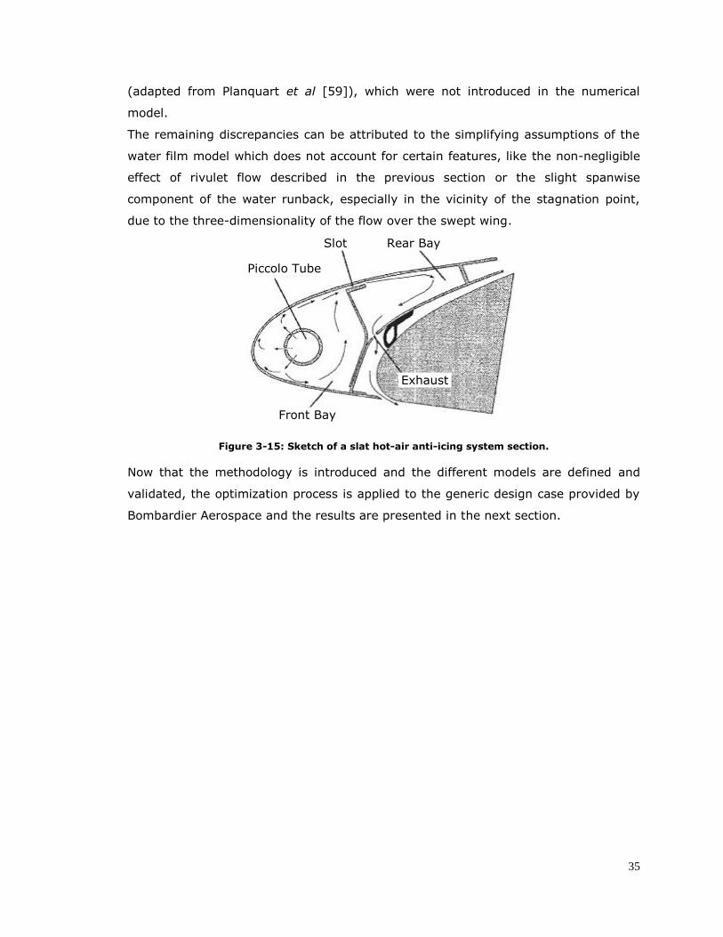
35
(adapted from Planquart et al [59]), which were not introduced in the numerical
model.
The remaining discrepancies can be attributed to the simplifying assumptions of the
water film model which does not account for certain features, like the non-negligible
effect of rivulet flow described in the previous section or the slight spanwise
component of the water runback, especially in the vicinity of the stagnation point,
due to the three-dimensionality of the flow over the swept wing.
Figure 3-15: Sketch of a slat hot-air anti-icing system section.
Now that the methodology is introduced and the different models are defined and
validated, the optimization process is applied to the generic design case provided by
Bombardier Aerospace and the results are presented in the next section.
Exhaust
Rear Bay
Front Bay
Piccolo Tube
Slot

36
4. APPLYING THE OPTIMIZATION METHODOLOGY
4.1 Genetic Algorithm’s Convergence
Figure 4-1 illustrates the typical convergence behavior of the genetic algorithms.
a
Generation
Fitnes
s val
ue
Mean & best fitness value
aaa
Generation
Fitnes
s val
ue
Mean & best fitness value
b
Generation
Mea
n d
ista
nce
Mean distance b/w individuals
b
Generation
Mea
n d
ista
nce
Mean distance b/w individuals
c
Generation
Fitnes
s val
ue
Mean & range of fitness value
c
Generation
Fitnes
s val
ue
Mean & range of fitness value
Figure 4-1: Genetic algorithm’s convergence.
The red dots in Picture (a) show the evolution of the best individual from generation
to generation, which gradually converges towards the global optimum. The blue dots
represent the average of the population, which also gradually evolves towards the
best individual. In Picture (b) the mean distance between individuals tends to
decrease as the generation number grows. In fact, the population is initially
uniformly distributed across the design space using the Lp-τ method and will

37
gradually contract and converge towards the global optimum, as summarized in
Picture (c) which shows the evolution of the mean value and range of the population
with the generations. Note that a gap in the mean distance or the range of fitness
value between two consecutive generations, like between generations 17 and 18 in
Figure 4-1, can be explained as the result of stochastic mutations (cf. section 3.2.2).
As a lower-dimension analogy, easier to visualize, a simpler 2D optimization example
with a relatively simple arbitrarily chosen objective function containing a global
optimum and a local one is presented in Figure 4-2.
Figure 4-2: 2D optimization example.
Figure 4-3: Initial population uniformly spread using Lp-τ.

38
The GA initial population (in this case 23 individuals) is first uniformly distributed
over the design space, as shown in Figure 4-3. The GA processes unfold with the
generations. Partial convergence is shown at generation #5 and #8 in Figure 4-4 and
the finally converged population is obtained for generation #12, as shown in Figure
4-5.
Figure 4-4: Partial GA convergence.
Figure 4-5: Final GA convergence.
In order to illustrate the subtleties of Piccolo tube optimization with fixed available
anti-icing power, Figure 4-6 presents three Piccolo tube configurations (cf. Pictures
denoted by -a) with their associated water runback solutions (cf. Pictures denoted by
-b).

39
1a 1b1a1a 1b1b
2a2b
2a2a2b2b
3a 3b3a3a 3b3b
Figure 4-6: Optimal design configuration versus slightly off-design configurations.
In this study, the given anti-icing enthalpy seemed to be inadequate to achieve fully
evaporative in any configuration within the range of the design variables. Therefore,
the lower surface minimum water runback criterion, mentioned in section 3.3.3, was
used.

40
The second configuration in Picture (2a) refers to the optimal geometric configuration
in the case of 3 design variables (jet angles and distance between holes). It shows
fully evaporative conditions by the end of the upper heated surface with minimal
runback out of the lower heated surface, as shown in Picture (2b). Configurations (1)
and (3) correspond to slight variations about the optimal point. On the one hand, the
first configuration (cf. Picture (1a)) leads to stronger evaporative conditions on the
upper heated surface, but to more runback on the lower heated surface (cf. Picture
(1b)). On the other hand, the third configuration (cf. Picture (3a)) leads to water
runback on both upper and lower surfaces (cf. Picture (3b)). It is important pointing
out that, for all three configurations, the available anti-icing power (i.e. the Piccolo
tube air temperature and mass flow rate) is identical.
The optimization results for 3, 4 and 5 design variables presented in the following
sections for different arrangements are compared to the initial generic geometric
configuration and water film results (cf. configuration #0 in Figure 4-7).
Figure 4-7: Initial generic configuration and corresponding water runback.
These results are the optimal geometric configurations obtained in the context of this
particular single objective optimization and within the range of the design variables.
Also, the following results represent a mean of 3 to 5 GA results in order to better
represent the coherence of the results and level down the slight variations in the
results introduced by the non-deterministic nature of genetic algorithms.
4.2 3-Design-Variable Configurations
The first arrangement for 3 design variables consists of the two jet angles and the
distance between holes (cf. configuration #1 in Figure 4-8). The second arrangement
for 3 design variables consists of one jet angle (keeping a 30° opening between the
two rows) and the x- and y- positions of the Piccolo tube (cf. configuration #2 in
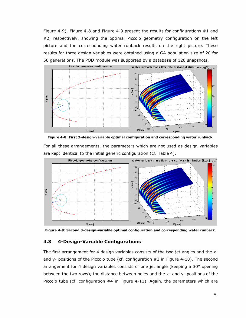
41
Figure 4-9). Figure 4-8 and Figure 4-9 present the results for configurations #1 and
#2, respectively, showing the optimal Piccolo geometry configuration on the left
picture and the corresponding water runback results on the right picture. These
results for three design variables were obtained using a GA population size of 20 for
50 generations. The POD module was supported by a database of 120 snapshots.
Figure 4-8: First 3-design-variable optimal configuration and corresponding water runback.
For all these arrangements, the parameters which are not used as design variables
are kept identical to the initial generic configuration (cf. Table 4).
Figure 4-9: Second 3-design-variable optimal configuration and corresponding water runback.
4.3 4-Design-Variable Configurations
The first arrangement for 4 design variables consists of the two jet angles and the x-
and y- positions of the Piccolo tube (cf. configuration #3 in Figure 4-10). The second
arrangement for 4 design variables consists of one jet angle (keeping a 30° opening
between the two rows), the distance between holes and the x- and y- positions of the
Piccolo tube (cf. configuration #4 in Figure 4-11). Again, the parameters which are
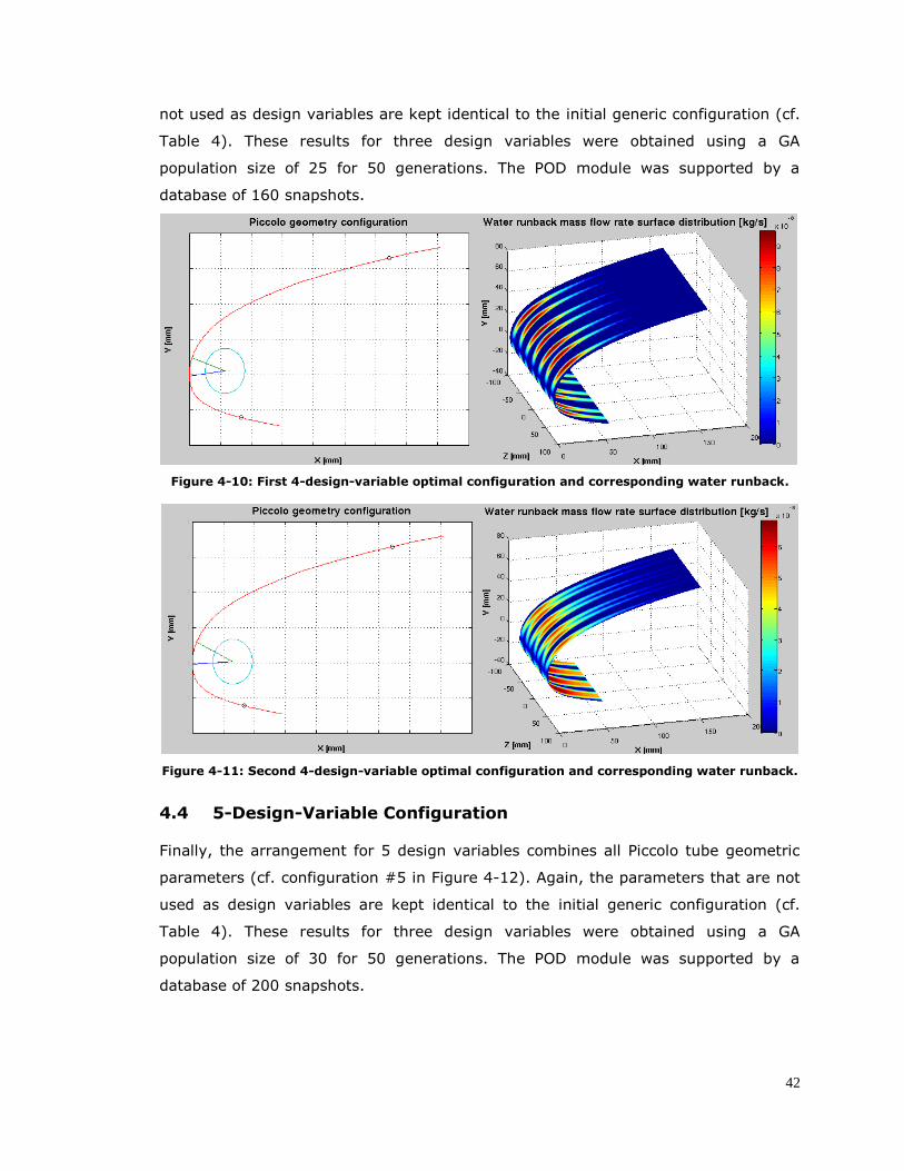
42
not used as design variables are kept identical to the initial generic configuration (cf.
Table 4). These results for three design variables were obtained using a GA
population size of 25 for 50 generations. The POD module was supported by a
database of 160 snapshots.
Figure 4-10: First 4-design-variable optimal configuration and corresponding water runback.
Figure 4-11: Second 4-design-variable optimal configuration and corresponding water runback.
4.4 5-Design-Variable Configuration
Finally, the arrangement for 5 design variables combines all Piccolo tube geometric
parameters (cf. configuration #5 in Figure 4-12). Again, the parameters that are not
used as design variables are kept identical to the initial generic configuration (cf.
Table 4). These results for three design variables were obtained using a GA
population size of 30 for 50 generations. The POD module was supported by a
database of 200 snapshots.
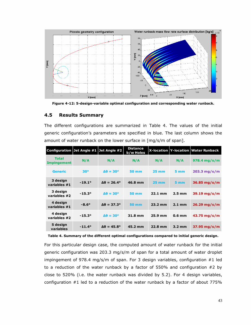
43
Figure 4-12: 5-design-variable optimal configuration and corresponding water runback.
4.5 Results Summary
The different configurations are summarized in Table 4. The values of the initial
generic configuration’s parameters are specified in blue. The last column shows the
amount of water runback on the lower surface in [mg/s/m of span].
Configuration Jet Angle #1 Jet Angle #2Distance
b/w HolesX-location Y-location Water Runback
Total
ImpingementN/A N/A N/A N/A N/A 978.4 mg/s/m
Generic 30° Δθ = 30° 50 mm 25 mm 5 mm 203.3 mg/s/m
3 design
variables #1-19.1° Δθ = 26.4° 46.8 mm 25 mm 5 mm 36.85 mg/s/m
3 design
variables #2-15.3° Δθ = 30° 50 mm 22.1 mm 2.5 mm 39.19 mg/s/m
4 design
variables #1-8.6° Δθ = 37.3° 50 mm 23.2 mm 2.1 mm 26.29 mg/s/m
4 design
variables #2-15.3° Δθ = 30° 31.8 mm 25.9 mm 0.6 mm 43.75 mg/s/m
5 design
variables-11.4° Δθ = 45.8° 45.2 mm 22.8 mm 3.2 mm 37.95 mg/s/m
Table 4. Summary of the different optimal configurations compared to initial generic design.
For this particular design case, the computed amount of water runback for the initial
generic configuration was 203.3 mg/s/m of span for a total amount of water droplet
impingement of 978.4 mg/s/m of span. For 3 design variables, configuration #1 led
to a reduction of the water runback by a factor of 550% and configuration #2 by
close to 520% (i.e. the water runback was divided by 5.2). For 4 design variables,
configuration #1 led to a reduction of the water runback by a factor of about 775%

44
and configuration #2 by 465%. Finally, for 5 design variables, the obtained optimal
configuration led to a reduction of the water runback by a factor of 535%.
Considering a more coherent way to look at the results by comparing only the related
configurations gives an interesting perspective regarding the consistency of the
results. Logically, releasing an additional degree of freedom, i.e. adding a design
variable, will lead to a “better” optimum. Actually, the optimal configuration of the
subspace might only be a local optimum of the higher-dimension space. It is the
most probable case since the subspace is constrained arbitrarily with respect to the
remaining design variables. This improvement of the optimal configuration was in
fact experienced when progressing from three to four design variables (cf. Table 5).
Configuration Jet Angle #1 Jet Angle #2Distance
b/w HolesX-location Y-location Water Runback
Total
ImpingementN/A N/A N/A N/A N/A 978.4 mg/s/m
Generic 30° Δθ = 30° 50 mm 25 mm 5 mm 203.3 mg/s/m
3 design
variables-15.3° Δθ = 30° 50 mm 22.1 mm 2.5 mm 39.19 mg/s/m
4 design
variables-8.6° Δθ = 37.3° 50 mm 23.2 mm 2.1 mm 26.29 mg/s/m
5 design
variables-11.4° Δθ = 45.8° 45.2 mm 22.8 mm 3.2 mm 37.95 mg/s/m
Table 5. Consecutive optimal configurations compared to initial generic design.
However, this was not satisfied for five design variables, even though the design was
greatly improved with respect to the generic configuration (in the context of this
single objective optimization) and still better than the 3-design-variable optimal
configuration.
Unfortunately, releasing an additional degree of freedom expands the size of the
design space whose accurate exploration is thus made more difficult as more POD
snapshots would be needed. Also, it is important to keep in mind that the GA
procedure is based on POD approximate evaluations which can introduce increasing
error with the number of dimensions and mislead GA convergence. This is in relation
to the Kriging interpolation method as well, which contains non-deterministic
components and gets more delicate to perform with increasing number of dimension
and associated increasing non-linearity of the problem. Not only that, but also the set
of POD snapshots used for three, four and five design variables was different by
definition since discretizing different subspaces. This would affect the optimization
process by modifying the way the physical features are incorporated into the POD

45
model. Another related aspect concerns the repeatability of the genetic algorithm
which is intrinsically non-deterministic. In any case, there is also a compromise
between accuracy and computational cost since increasing the population size will
help the exploration of the design space and increase the consistency of the model,
while increasing the number of generations will improve the convergence level and
the consistency and repeatability of the results, at least as far as the genetic
algorithm is concerned, but certainly at the cost of additional computations.
Here, the optimization was not done sequentially, since for each of these
configurations the GA was re-initialized to a uniformly distributed initial population.
However, sequential optimization was investigated with moderate results. Indeed,
starting from the lower-dimension optimal GA population results would not
necessarily lead to significant improvement, even if the population is uniformly
spread in the supplementary dimension. This bias in the GA initial population could
lead to the convergence towards a local optimum and therefore would not guaranty
convergence towards the best possible optimum of the constrained design space. It
would even result in a more laborious convergence, since it would require a higher
rate of mutation to recover the necessary diversity in the population.
As a lower-dimension analogy, a simpler 2D optimization example with a relatively
simple arbitrarily chosen objective function containing a global optimum and a local
one was implemented (cf. Appendix D) and the trends mentioned above were
verified.
In order to clarify this matter, the optimization methodology was run for five design
variables without the POD-Kriging module, with the Genetic Algorithm module
directly linked to the water film solver. It led to a clear convergence towards a much
more consistent result (885% improvement in terms of water runback), as shown in
Table 6.
Configuration Jet Angle #1 Jet Angle #2Distance
b/w HolesX-location Y-location Water Runback
Total
ImpingementN/A N/A N/A N/A N/A 978.4 mg/s/m
Generic 30° Δθ = 30° 50 mm 25 mm 5 mm 203.3 mg/s/m
5 design
variables
w/o POD
-17.8° Δθ = 36.6° 74.4 mm 23.6 mm 1.1 mm 23.03 mg/s/m
Table 6. Optimal configuration obtained without POD.
The optimal Piccolo geometric configuration and associated water runback solution is
presented in Figure 4-13.
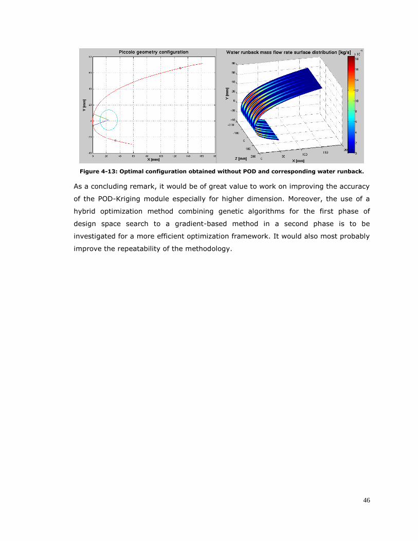
46
Figure 4-13: Optimal configuration obtained without POD and corresponding water runback.
As a concluding remark, it would be of great value to work on improving the accuracy
of the POD-Kriging module especially for higher dimension. Moreover, the use of a
hybrid optimization method combining genetic algorithms for the first phase of
design space search to a gradient-based method in a second phase is to be
investigated for a more efficient optimization framework. It would also most probably
improve the repeatability of the methodology.

47
CONCLUSION AND FUTURE WORK
This work tries to bring some rigor to a field long governed by trial-and-error and
empiricism. It presents an optimization methodology for anti-icing systems based on
3D CFD computations and combining powerful tools such as a genetic evolutionary
algorithm, which is ideal for searching multi-dimensional design space, and a POD-
based Reduced-Order Model allowing to greatly reducing the computational cost.
Being thus affordable and modular, this optimization method is promising and
adaptable to handle more complex 3D geometries and physics. This method was
successfully applied and led to optimal geometric configurations for 3- to 5-
dimensional design spaces, improving the initial generic design by up to 885%.
In terms of future developments, geometric shape and Piccolo power inputs
variations in the spanwise direction can be taken into account, as well as wing tip and
root effects. The ROM module can be upgraded to improve accuracy. Moreover, the
correlation can be upgraded back to a 3D CFD computation, while the water film
model could be replaced by the ICE3D module of FENSAP-ICE.
Concerning the handling of several design points (external conditions), the method
can still be applied with an adaptation of the objective function to account for the
additional constraints or with the construction of a Pareto front in a multi-objective
optimization framework.
Further research could focus on applying the Reduced-Order Model directly to fully
coupled computations constituting the snapshots, and running the genetic algorithm
module with such a higher-fidelity POD model. An interesting future application would
be to adapt this method to electro-thermal anti-icing systems.
In addition to the new technical skills that I acquired and perfected throughout this
project, in thermodynamics, CFD, optimization and Reduced-Order Modelling, this
experience constituted a personal challenge which I am particularly proud to have
accomplished.

48
REFERENCES
[1] National Transportation Safety Board, Annual Review of Aircraft Accident Data, U.S. General Aviation, 2005.
[2] K. R. Petty, and C. D. J. Floyd, "A Statistical Review of Aviation Airframe Icing
Accidents in the US," 11th ASM Conference on Aviation, Range, and Aerospace, Hyannis, MA, USA, 2004.
[3] European Aviation Safety Agency, Annual Safety Review 2007, EASA, 2007. [4] S. G. Cober, and G. A. Isaac, "Aircraft Icing Environments Observed In Mixed-Phase
Clouds," 40th AIAA Aerospace Sciences Meeting and Exhibit, AIAA-2002-675, Reno, NV, USA, 2002.
[5] Federal Aviation Administration, General Aviation Safety Challenges 2008 - Part 2,
FAA, 2008. [6] United States Department of Transportation, In-Flight Aircraft Icing Plan, FAA, 1997. [7] Civil Aviation Authority of New Zealand, Aircraft Icing Handbook, Lower Hutt, New
Zealand, 2000.
[8] I. Paraschivoiu, and M. T. Brahimi, Aircraft In-Flight Icing, Centre de Développement Technologique, École Polytechnique de Montréal, Montreal, QC, Canada, 1997.
[9] G. Mingione, and M. Barocco, Flight in Icing Conditions Summary, French DGAC, 1997. [10] M. G. Potapczuk, "A Review of NASA Lewis' Development Plans for Computational
Simulation of Aircraft Icing," AIAA Paper, AIAA–1999–243, 1999. [11] J. Steuernagle, K. Roy, and D. Wright, Safety Advisor : Aircraft Icing, AOPA Air Safety
Foundation, 2008. [12] Federal Aviation Administration, Airworthiness Standards: Transport Category
Airplanes, Part 25, Appendix C, FAA, 2007.
[13] European Aviation Safety Agency, Certification Specifications for Large Aeroplanes CS-25, Appendix C, EASA, 2003.
[14] Transport Canada. "Canadian Aviation Regulations 2009-2," http://www.tc.gc.ca/civilaviation/regserv/affairs/cars/menu.htm.
[15] K. E. Yeoman, "Efficiency of a Bleed Air Powered Inlet Icing Protective System," 32nd AIAA Aerospace Sciences Meeting and Exhibit, AIAA-1994-717, Reno, NV, USA, 1994.
[16] R. M. Norris, K. J. Rumford, and D. S. Youd, Anti-icing valve United States Patent
4831819,to Avco Corporation (Providence, RI) 1989. [17] K. M. Al-Khalil, T. G. Keith Jr., and K. J. De Witt, “New Concept in Runback Water
Modeling for Anti-Iced Aircraft Surfaces,” Journal of Aircraft, vol. 30, no. 1, pp. 41-49, 1993.
[18] K. M. Al-Khalil, T. G. Keith Jr., and K. J. De Witt, “Development of an Improved Model for Runback Water on Aircraft Surfaces,” Journal of Aircraft, vol. 31, no. 2, pp. 271-
278, 1994. [19] G. Fortin, A. Ilinca, J.-L. Laforte, and V. Brandi, “New Roughness Computation Method
and Geometric Accretion Model for Airfoil Icing,” Journal of Aircraft, vol. 41, no. 1, pp. 119-127, 2004.
[20] G. Fortin, J.-L. Laforte, A. Ilinca, and V. Brandi, "Prediction of 2D Airfoil Ice Accretion by Bisection Method and by Rivulets and Beads Modeling," 39th Aerospace Sciences Meeting and Exhibit, AIAA-2003-1076, Reno, NV, USA, 2003.
[21] B. L. Messinger, “Equilibrium Temperature of an Unheated Icing Surface as a Function of Airspeed,” Journal of Aeronautical Sciences, vol. 20, no. 1, pp. 29-42, 1953.
[22] T. G. Myers, “Extension to the Messinger Model for Aircraft Icing,” AIAA Journal, vol. 39, no. 2, pp. 211-218, 2001.
[23] T. G. Myers, J. P. F. Charpin, and S. J. Chapman, “The Flow and Solification of a Thin Fluid Film on an Arbitrary Three-Dimensional Surface,” Journal of Phisics of Fluids, vol. 14, no. 8, pp. 2788-2803, 2002.
[24] T. G. Myers, and C. P. Thompson, “Modeling the Flow of Water on Aircraft in Icing Conditions,” AIAA Journal, vol. 36, no. 6, pp. 1010-1013, 1998.
[25] C. N. Donatti, R. A. Silveira, C. R. Maliska, and A. F. C. da Silva, "Ice Accretion Simulation in Presence of a Hot Air Anti-Icing System," 19th COBEM International Congress of Mechanical Engineering, Brasília, DF, Brazil, 2007.
49
[26] O. Harireche, P. Verdin, C. P. Thompson, and D. W. Hammond, “Explicit Finite Volume
Modeling of Aircraft Anti-Icing and De-Icing,” Journal of Aircraft, vol. 45, no. 6, pp. 1924-1936, 2008.
[27] S. Kato, “Solution for Aircraft Anti-Icing System Simulation by a Modified Perturbation Method,” Journal of Aircraft, vol. 43, no. 2, pp. 544-554, 2006.
[28] G. A. Lima da Silva, O. de Mattos Silvares, and E. J. Godoy de Jesus Zerbini, "Simulation of an Airfoil Electro-Thermal Anti-Ice System Operating in Running Wet Regime," 43rd AIAA Aerospace Sciences Meeting and Exhibit, AIAA 2005-1374, Reno, NV, USA, 2005.
[29] G. A. Lima da Silva, O. de Mattos Silvares, and E. J. Godoy de Jesus Zerbini, “Numerical Simulation of Airfoil Thermal Anti-Ice Operation, Part 1: Mathematical Modeling,” Journal of Aircraft, vol. 44, no. 2, pp. 627-634, 2007.
[30] G. A. Lima da Silva, O. de Mattos Silvares, and E. J. Godoy de Jesus Zerbini, “Numerical Simulation of Airfoil Thermal Anti-Ice Operation, Part 2: Implementation and Results,” Journal of Aircraft, vol. 44, no. 2, pp. 635-641, 2007.
[31] F. Morency, M. T. Brahimi, F. Tezok, and I. Paraschivoiu, "Hot Air Anti-Icing System Modelization in the Ice Prediction Code CANICE," 36th AIAA Aerospace Sciences
Meeting and Exhibit, AIAA-1998-192, Reno, NV, USA, 1998.
[32] F. Morency, F. Tezok, and I. Paraschivoiu, “Anti-Icing System Simulation Using CANICE,” Journal of Aircraft, vol. 36, no. 6, pp. 999-1006, 1999.
[33] F. Morency, F. Tezok, and I. Paraschivoiu, “Heat and Mass Transfer in the Case of Anti-Icing System Simulation,” Journal of Aircraft, vol. 37, no. 2, pp. 245-252, 2000.
[34] F. Saeed, “State-of-the-Art Aircraft Icing and Anti-Icing Simulation,” ARA Journal, vol. 2000-2002, no. 25-27, pp. 106-113, 2003.
[35] H. Wang, “3D Conjugate Heat Transfer Simulation of Aircraft Hot-Air Anti-Icing
Systems,” Masters Thesis, Mechanical Engineering, McGill University, Montreal, QC, Canada, 2005.
[36] J. Lee, D. Rigby, W. Wright, and Y. Choo, "Analysis of Thermal Ice Protection System (TIPS) with Piccolo Tube using State-of-the-Art Software," 44th AIAA Aerospace Sciences Meeting and Exhibit, AIAA-2006-1011, Reno, NV, USA, 2006.
[37] K. M. Al-Khalil, T. G. Keith Jr., and K. J. De Witt, “Icing Calculations on a Typical Commercial Jet Engine Inlet Nacelle,” Journal of Aircraft, vol. 34, no. 1, pp. 87-93,
1997.
[38] A. Pueyo, F. Mokhtarian, and F. Kafyeke, "Validation of a Hot-Air Anti-icing Simulation Code," World Aviation Congress & Exposition, SAE, Montreal, QC, Canada, 2003.
[39] F. Saeed, F. Morency, and I. Paraschivoiu, "Numerical Simulation of a Hot-Air Anti-Icing System," 38th AIAA Aerospace Sciences Meeting and Exhibit, AIAA-2000-630, Reno, NV, USA, 2000.
[40] C. N. Aliaga Rivera, “An Unsteady Multiphase Approach to In-Flight Icing,” Maters Thesis, Mechanical Engineering, McGill University, Montreal, QC, Canada, 2008.
[41] K. Nakakita, S. Nadarajah, and W. G. Habashi, “Towards Real-Time Aero-Icing Simulation of Complete Aircraft, via FENSAP-ICE,” Journal of Aircraft, vol. 47, no. 1, pp. 96-109, 2010.
[42] H. Wang, P. Tran, W. G. Habashi, Y. Chen, M. Zhang, and L. Feng, "Anti-Icing Simulation in Wet Air of a Piccolo System using FENSAP-ICE," 2007 SAE Aircraft and
Engine Icing International Conference, Seville, Spain, 2007. [43] H. Beaugendre, “A PDE-Based 3D Approach to In-Flight Ice Accretion,” Ph.D. Thesis,
Mechanical Engineering, McGill University, Montreal, QC, Canada, 2003. [44] Y. Bourgault, H. Beaugendre, and W. G. Habashi, “Development of a Shallow-Water
Icing Model in FENSAP-ICE,” Journal of Aircraft, vol. 37, no. 4, pp. 640-646, 2000. [45] G. F. Croce, W. G. Habashi, G. Guevremont, and F. Tezok, "3D Thermal Analysis of an
Anti-Icing Device Using FENSAP-ICE," 36th AIAA Aerospace Sciences Meeting and
Exhibit, AIAA-1998-193, Reno, NV, USA, 1998. [46] W. G. Habashi, “Recent Advances in CFD for In-Flight Icing Simulation,” Japan Society
of Fluid Mechanics, vol. 28, no. 2, pp. 99-118, 2009. [47] G. A. Lima da Silva, O. de Mattos Silvares, and E. J. Godoy de Jesus Zerbini, "Water
Film Breakdown and Rivulets Formation Effects on Thermal Anti-Ice Operation Simulation," 9th AIAA/ASME Joint Thermophysics and Heat Transfer Conference, AIAA-
2006-3785, San Francisco, CA, USA, 2006.

50
[48] D. Wang, G. F. Naterer, and G. Wang, “Thermofluid Optimization of a Heated
Helicopter Engine Cooling-Bay Surface,” Canadian Aeronautics and Space Journal, vol. 49, no. 2, pp. 73-86, 2003.
[49] J. M. Brown, S. Raghunathan, J. K. Watterson, A. J. Linton, and D. Riordon, “Heat Transfer Correlation for Anti-Icing Systems,” Journal of Aircraft, vol. 39, no. 1, pp. 65-
70, 2002. [50] B. S. de Mattos, and G. L. Oliveira, "Three-Dimensional Thermal Coupled Analysis of a
Wing Slice Slat with a Piccolo Tube," 18th AIAA Applied Aerodynamics Conference, AIAA-2000-3921, Denver, CO, USA, 2000.
[51] M. Fregeau, M. Gabr, F. Saeed, and I. Paraschivoiu, "Numerical Simulation of Heat Transfer from an Array of Hot-Air Jets Impinging on a 3D Concave Surface," 50th CASI Annual General Meeting & Conference, Montreal, QC, Canada, 2003.
[52] M. Fregeau, F. Saeed, and I. Paraschivoiu, “Numerical Heat Transfer Correlation for Array of Hot-Air Jets Impinging on 3-Dimensional Concave Surface,” Journal of Aircraft, vol. 42, no. 3, pp. 665-670, 2005.
[53] J. Hua, F. Kong, and H. H. T. Liu, “Unsteady Thermodynamic Computational Fluid Dynamics Simulations of Aircraft Wing Anti-Icing Operation,” Journal of Aircraft, vol.
44, no. 4, pp. 1113-1117, 2007.
[54] J. Hua, and H. H. T. Liu, “Fluid Flow and Thermodynamic Analysis of a Wing Anti-Icing System,” Canadian Aeronautics and Space Journal, CASI, vol. 51, no. 1, pp. 35-40, 2005.
[55] H. H. T. Liu, and J. Hua, “Three-Dimensional Integrated Thermodynamic Simulation for Wing Anti-Icing System,” Journal of Aircraft, vol. 41, no. 6, pp. 1291-1297, 2004.
[56] S. Özgen, and M. Canibek, “Ice Accretion Simulation on Multi-Element Airfoils Using Extended Messinger Model,” Heat and Mass Transfer, vol. 45, pp. 305-322, 2009.
[57] M. Papadakis, S.-H. Wong, H.-W. Yeong, S.-C. Wong, and G. T. Vu, "Icing Tunnel Experiments with a Hot Air Anti-Icing System," 46th AIAA Aerospace Sciences Meeting and Exhibit, AIAA-2008-444, Reno, NV, USA, 2008.
[58] M. Papadakis, and S.-H. J. Wong, "Parametric Investigation of a Bleed Air Ice Protection System," 44th AIAA Aerospace Sciences Meeting and Exhibit, AIAA-2006-1013, Reno, NV, USA, 2006.
[59] P. Planquart, G. Vanden Borre, and J.-M. Buchlin, "Experimental and Numerical
Optimization of a Wing Leading Edge Hot Air Anti-icing System," 43rd AIAA Aerospace
Sciences Meeting and Exhibit, AIAA-2005-1277, Reno, NV, USA, 2005. [60] D. Rigby, "Numerical Investigation of Hole Pattern Effect on Piccolo Tube Anti-Icing,"
44th AIAA Aerospace Sciences Meeting and Exhibit, AIAA-2006-1012, Reno, NV, USA, 2006.
[61] S. J. Riley, and E. H. James, "Investigations Relating to the Effects of Various Internal
Geometries on the Effectiveness of an Aero-Engine Intake Thermal Anti-Icing System," 39th ASME International Gas Turbine & Aeroengine Congress & Exposition, The Hague, Netherlands, 1994.
[62] F. Saeed, and A. Z. Al-Garni, “Numerical Simulation of Surface Heat Transfer from an Array of Hot-Air Jets,” Journal of Aircraft, vol. 45, no. 2, pp. 700-714, 2008.
[63] E. A. Whalen, A. P. Broeren, M. B. Bragg, and S. Lee, "Characteristics of Runback Ice Accretions on Airfoils and their Aerodynamic Effects," 43rd AIAA Aerospace Science
Meeting and Exhibit, AIAA-2005-1065, Reno, NV, USA, 2005. [64] S.-H. Wong, M. Papadakis, and A. Zamora, "Computational Investigation of a Bleed Air
Ice Protection System," 1st AIAA Atmospheric and Space Environments Conference, AIAA-2009-3966, San Antonio, Texas, USA, 2009.
[65] W. B. Wright, "An Evaluation of Jet Impingement Heat Transfer Correlations for Piccolo Tube Application," 42nd AIAA Aerospace Sciences Meeting and Exhibit, AIAA-2004-62, Reno, NV, USA, 2004.
[66] R. J. Goldstein, A. I. Behbahani, and K. Kieger Heppelmann, “Streamwise Distribution of the Recovery Factor and the Local Heat Transfer Coefficient to an Impinging Circular Air Jet,” Int. J. Heat and Mass Transfer, vol. 29, no. 8, pp. 1227-1235, 1986.
[67] R. Gardon, and J. C. Akfirat, “The Role of Turbulence in Determining the Heat-Transfer Characteristics of Impinging Jets,” Int. J. Heat and Mass Transfer, vol. 8, pp. 1261-1272, 1965.

51
[68] K. Jambunathan, M. A. Moss, and B. L. Button, “A Review of Heat Transfer Data for
Single Circular Jet Impingement,” Int. J. Heat and Fluid Flow, vol. 13, no. 2, pp. 106-115, 1992.
[69] L. Huang, and M. S. El-Genk, “Heat Transfer of an Impinging Jet on a Flat Surface,” Int. J. Heat and Mass Transfer, vol. 37, no. 13, pp. 1915-1923, 1994.
[70] A. A. Tawfek, “Heat Transfer and Pressure Distributions of an Impinging Jet on a Flat Plate,” Heat and Mass Transfer, vol. 32, no. 1-2, pp. 49-54, 1996.
[71] M. Angioletti, R. M. Di Tommaso, E. Nino, and G. Ruocco, “Simultaneous Visualization of Flow Field and Evaluation of Local Heat Transfer by Transitional Impinging Jets,” Int. J. Heat and Mass Transfer, vol. 46, no. 10, pp. 1703-1713, 2003.
[72] A. M. Huber, and R. Viskanta, “Effect of Jet-Jet Spacing on Convective Heat Transfer to Confined, Impinging Arrays of Axisymmetric Air Jets,” Int. J. Heat and Mass Transfer,
vol. 37, no. 18, pp. 2859-2869, 1994. [73] D.-H. Rhee, P.-H. Yoon, and H. H. Cho, “Local Heat/Mass Transfer and Flow
Characteristics of Array Impinging Jets with Effusion Holes Ejecting Spent Air,” Int. J. Heat and Mass Transfer, vol. 46, no. 6, pp. 1049-1061, 2003.
[74] J.-Y. San, and M.-D. Lai, “Optimum Jet-to-Jet Spacing of Heat Transfer for Staggered
Arrays of Impinging Air Jets,” Int. J. Heat and Mass Transfer, vol. 44, no. 21, pp.
3997-4007, 2001. [75] B. V. N. Rama Kumar, and B. V. S. S. S. Prasad, “Computational Flow and Heat
Transfer of a Row of Circular Jets Impinging on a Concave Surface,” Heat and Mass Transfer, vol. 44, no. 6, pp. 667-678, 2008.
[76] L. C. d. C. Santos, R. H. Domingos, R. B. Maria, and M. d. F. Leal, "Sensitivity Analysis of a Bleed Air Anti-Ice Thermal Model to Geometrical and Operational Parameters," 46th AIAA Aerospace Sciences Meeting and Exhibit, AIAA-2008-445, Reno, NV, USA,
2008. [77] F. Saeed, and I. Paraschivoiu, "Optimization of a Hot-Air Anti-Icing System," 41st AIAA
Aerospace Sciences Meeting and Exhibit, AIAA-2003-733, Reno, NV, USA, 2003. [78] Bombardier Aerospace proprietary data, 2009. [79] H.-S. Chung, and J. J. Alonso, "Multiobjective Optimization Using Approximation
Model-based Genetic Algorithms," 10th AIAA/ISSMO Symposium on Multidisciplinary Analysis and Optimization, AIAA-2004-4325, Albany, NY, USA, 2004.
[80] H. Arizono, and K. Isogai, “Application of Genetic Algorithm for Aeroelastic Tailoring of
a Cranked-Arrow Wing,” Journal of Aircraft, vol. 42, no. 2, pp. 493-499, 2005. [81] A. Saario, A. Oksanen, and M. Ylitalo, “Combination of Genetic Algorithm and
Computational Fluid Dynamics in Combustion Process Emission Minimization,” Combustion Theory and Modelling, vol. 10, no. 6, pp. 1037-1047, 2006.
[82] Y. Tahara, S. Tohyama, and T. Katsui, “CFD-based Multi-Objective Optimization
Method for Ship Design,” International Journal for Numerical Methods in Fluids, vol. 52, no. 5, pp. 499-527, 2006.
[83] A. Kumar, A. J. Keane, P. B. Nair, and S. Shahpar, "Efficient Genetic Algorithm Based Robust Design Method for Compressor Fan Blades," ASME 2005 International Design Engineering Technical Conferences & Computers and Information in Engineering Conference, Long Beach, CA, USA, 2005.
[84] S. Jeong, M. Murayama, and K. Yamamoto, “Efficient Optimization Design Method
Using Kriging Model,” Journal of Aircraft, vol. 42, no. 2, pp. 413-420, 2005. [85] L. Padovan, V. Pediroda, and C. Poloni, Multi Objective Robust Design Optimization of
Airfoils in Transonic Field, pp. 283-295, Springer, 2005. [86] R. A. Van den Braembussche, "Evolutive Methods : Theoretical Aspects & Definitions,"
NATO Research and Technology Organization Lecture Series (AVT-167) on "Strategies for Optimization and Automated Design of Gas Turbine Engines", Montreal, Canada, October 26-27, 2009.
[87] I. Lepot, "Introduction and Terminology," NATO Research and Technology Organization Lecture Series (AVT-167) on "Strategies for Optimization and Automated Design of Gas Turbine Engines", Montreal, Canada, October 26-27, 2009.
[88] L. Bernier, “A Genetic Algorithm with Self-Adaptive Niche Sizing,” Masters Thesis, Computer Science, McGill University, 1995.
[89] P. Haroun, “Genetic Algorithm and Data Visualization,” Masters Thesis, Computer
Science, McGill University, 1997.
52
[90] K. F. Man, K. S. Tang, and S. Kwong, “Genetic Algorithms : Concepts and
Applications,” IEEE Transactions on Industrial Electronics, vol. 43, no. 5, pp. 519-534, 1996.
[91] M. Srinivas, and L. M. Patnaik, “Genetic Algorithms : A Survey,” Computer, vol. 27, no. 6, pp. 17-26, 1994.
[92] D. Whitley, “A Genetic Algorithm Tutorial,” Statistics and Computing, vol. 4, no. 2, pp. 65-85, 1994.
[93] R. A. Van den Braembussche, "Tuning of Optimization Strategies," NATO Research and Technology Organization Lecture Series (AVT-167) on "Strategies for Optimization and Automated Design of Gas Turbine Engines", Montreal, Canada, October 26-27, 2009.
[94] J. Burkardt, M. Gunzburger, and H.-C. Lee, “POD and CVT-based Reduced-Order Modeling of Navier-Stokes Flows,” Computer Methods in Applied Mechanics and
Engineering, vol. 196, no. 1-3, pp. 337-355, 2006. [95] G. Li, M. Li, S. Azarm, J. Rambo, and Y. Joshi, “Optimizing Thermal Design of Data
Center Cabinets with a New Multi-Objective Genetic Algorithm,” Distributed and Parallel Databases, vol. 21, no. 2-3, pp. 167-192, 2007.
[96] J. Favier, L. Cordier, A. Kourta, and A. Iollo, "Calibrated POD Reduced-Order Models of
Massively Separated Flows in the Perspective of their Control," ASME Joint U.S. -
European Fluids Engineering Summer Meeting, Miami, FL, USA, 2006. [97] J. Rambo, and Y. Joshi, "Reduced Order Modeling of Steady Turbulent Flows Using the
POD," ASME Summer Heat Transfer Conference, San Francisco, CA, USA, 2005. [98] L. Sirovich, “Turbulence and the Dynamics of Coherent Structures - Part III : Dynamics
and Scaling,” Quarterly of Applied Mathematics, vol. 45, no. 3, pp. 583-590, 1987. [99] R. F. Coelho, P. Breitkopf, and C. Knopf-Lenoir, “Model Reduction for Multidisciplinary
Optimization - Application to a 2D Wing,” Structural and Multidisciplinary Optimization,
vol. 37, no. 1, pp. 29-48, 2008. [100] I. Lepot, "Complements on Surrogate Based Optimization for Engineering Design,"
NATO Research and Technology Organization Lecture Series (AVT-167) on "Strategies for Optimization and Automated Design of Gas Turbine Engines", Montreal, Canada, October 26-27, 2009.
[101] D. E. Raveh, “Computational-Fluid-Dynamics-Based Aeroelastic Analysis and Structural Design Optimization - a Researcher's Perspective,” Computer Methods in Applied
Mechanics and Engineering, vol. 194, no. 30-33, pp. 3453-3471, 2005.
[102] P. Bratley, and B. L. Fox, “Algorithm 659: Implementing Sobol's Quasirandom Sequence Generator,” ACM Transactions on Mathematical Software, vol. 14, no. 1, pp. 88-100, 1988.
[103] A. Chang, I. Izmailov, S. Rizzo, S. Wynter, O. Alexandrov, and C. Tong, Computer Experiments for Function Approximations, Lawrence Livermore National Laboratory,
Livermore, CA, USA, October 17, 2007. [104] A. Isaacs, Sampling Strategies for Computer Experiments, January 2004. [105] S. Joe, and F. Y. Kuo, “Remark on Algorithm 659: Implementing Sobol's Quasirandom
Sequence Generator,” ACM Transactions on Mathematical Software, vol. 29, no. 1, pp. 49-57, 2003.
[106] I. M. Sobol, “On the Systematic Search in a Hypercube,” SIAM Journal on Numerical Analysis, vol. 16, no. 5, pp. 790-793, 1979.
[107] R. B. Statnikov, and J. B. Matusov, Multicriteria Optimization and Engineering, p. 212, New York: Chapman & Hall, 1995.
[108] A. Chatterjee, “An Introduction to the Proper Orthogonal Decomposition,” Current Science, vol. 78, no. 7, pp. 808-817, 2000.
[109] P. Holmes, J. L. Lumley, and G. Berkooz, Turbulence, Coherent Structures, Dynamical Systems and Symmetry, pp. 86-117, New York: Cambridge University Press, 1996.
[110] Y. C. Liang, H. P. Lee, S. P. Lim, W. Z. Lin, K. H. Lee, and C. G. Wu, “Proper
Orthogonal Decomposition and its Applications - Part 1 : Theory,” Journal of Sound and Vibration, vol. 252, no. 3, pp. 527-544, 2002.
[111] L. Sirovich, “Turbulence and the Dynamics of Coherent Structures - Part I : Coherent Structures,” Quarterly of Applied Mathematics, vol. 45, no. 3, pp. 561-571, 1987.
[112] K. Nakakita, “Toward Real-Time Aero-Icing Simulation Using Reduced Order Models,” Mechanical Engineering, McGill, Spring 2007.

53
[113] K. Nakakita, S. Nadarajah, and W. G. Habashi, “Towards Real-Time Aero-Icing
Simulation of Complete Aircraft, via FENSAP-ICE,” Journal of Aircraft, vol. 47, no. 1, pp. 96-109, January-February 2010.
[114] V. Lappo, “POD-Kriging Approximations of Multi-Disciplinary CFD Simulation with Application to In-Flight Icing,” Mechanical Engineering, McGill, Montreal, Spring 2010.
[115] V. Lappo, and W. G. Habashi, "POD-Kriging Approximations of Multi-Disciplinary CFD Simulation with Application to In-Flight Icing," 17th Annual Conference of the CFD Society of Canada, CFDSC2009-6E3, Ottawa, ON, Canada, 2009.
[116] B. D. Matheis, and A. P. Rothmayer, "Numerical Simulation of Thin Air Driven Films," 40th AIAA Aerospace Sciences Meeting and Exhibit, AIAA-2002-525, Reno, NV, USA, 2002.

54
APPENDIX A
A. SENSITIVITY ANALYSIS OF THE IMPACT OF WALL TEMPERATURE
A.1. On External Flow
A sensitivity analysis was performed in order to assess the impact of the wall
boundary condition temperature level on the flow variables involved in the icing
phenomena.
For the same set of external conditions, different constant temperature distributions
(270 K to 300 K in increments of 5 K, and adiabatic wall condition, for a free-stream
temperature of 265 K) were imposed as wall boundary condition, as illustrated in
Figure A-1.
Figure A-1. Imposed wall temperature boundary conditions.
The following figures show the different relevant flow variable distributions extracted
along a 2D cut on the slat’s surface, tangent to the free-stream.
The pressure distribution at the wall is negligibly affected, as shown in Figure A-2.
The wall shear stress seems to be slightly more impacted, as shown in Figure A-3,
but the range of variations is contained within ±6% which is acceptable.

55
Figure A-2. Wall pressure distribution along the skin.
Figure A-3. Wall shear stress distribution along the skin.

56
Figure A-4. Convective heat flux distribution along the skin.
Figure A-5. Heat transfer coefficient distribution along the skin.

57
The convective heat flux distribution is obviously affected since the higher the
temperature at the wall, the higher the convective heat flux, as shown in Figure A-4.
The interesting aspect concerns the heat transfer coefficient distribution, computed
from the convective heat flux, divided by the difference between local wall
temperature and local adiabatic temperature. It is interesting to notice that the
higher the temperature difference between imposed and free-stream temperatures,
the lower the impact on the heat transfer coefficient distribution, as shown in Figure
A-5. From a maximum error of about 10% for a temperature difference of 5 K, the
distribution seems to converge towards a settled distribution, within ±0.5% after a
temperature difference of 30 K. Therefore, the external flow will be considered
unaffected as long as a temperature difference of at least 30 K is emphasized.
With respect to the variable related to the droplet impingement calculation, namely
the local liquid water content, collection efficiency and impinging mass flux
distributions, the impact of wall temperature level is negligible as illustrated in Figure
A-6, Figure A-7 and Figure A-8.
Figure A-6. Local liquid water content distribution along the skin.
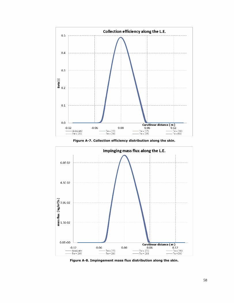
58
Figure A-7. Collection efficiency distribution along the skin.
Figure A-8. Impingement mass flux distribution along the skin.

59
A.2. On Internal Flow
Having in mind the recommendations from the external flow sensibility study, the
focus was oriented towards the impact on the internal heat transfer coefficient
distribution in order to have an idea of the error implied by the “uncoupling”
assumption. Thus, different wall temperature boundary conditions were imposed for
three test cases of 3D internal flow, as shown in Figure A-9:
1. a constant distribution at temperature level 288K
2. a constant distribution at temperature level 350K
3. a distribution somewhat similar to the temperature distribution obtained after
solving for the water film
In this case, the reference temperature is not the free-stream temperature nor the
adiabatic distribution but the Piccolo inlet temperature.
Figure A-9. Temperature boundary condition on the inner skin wall.
Figure A-10, Figure A-12 and Figure A-14 show the superposition of the heat transfer
coefficient distributions two by two, one in colors and the other one in black.
Figure A-11, Figure A-13 and Figure A-15 present the relative error distributions. The
maximum discrepancies are located at the neighboring of the jets stagnation points
but do not exceed 12% then quickly drops below 2%, for the two extreme cases
(cases 1 & 3) as shown in Figure A-11. Otherwise, it stands lower than 8% at the
picks and also quickly drops below 2%, as shown in Figure A-13 and Figure A-15.

60
These results satisfactorily validate the “uncoupling” assumption with reasonably low
impact on the internal heat transfer coefficient distribution.
Figure A-10. Heat transfer coefficient distribution on the inner skin wall for cases 1 & 3.
Figure A-11. Relative error distribution on the inner skin wall for cases 1 & 3.
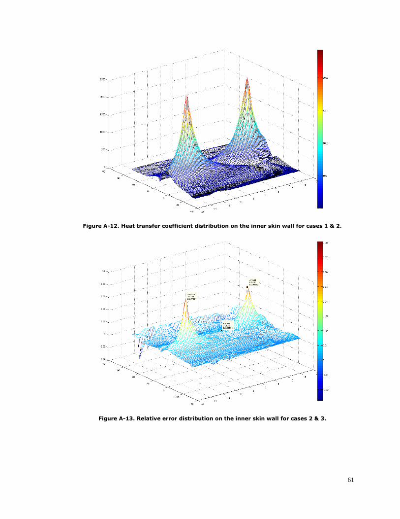
61
Figure A-12. Heat transfer coefficient distribution on the inner skin wall for cases 1 & 2.
Figure A-13. Relative error distribution on the inner skin wall for cases 2 & 3.
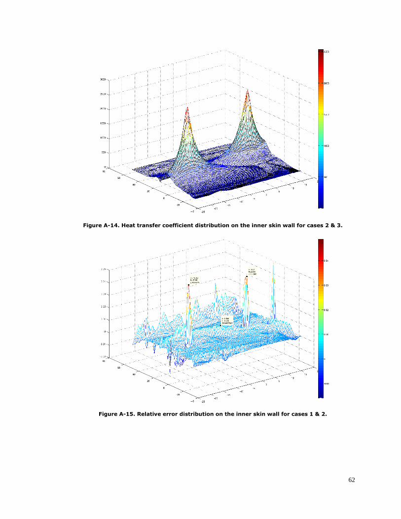
62
Figure A-14. Heat transfer coefficient distribution on the inner skin wall for cases 2 & 3.
Figure A-15. Relative error distribution on the inner skin wall for cases 1 & 2.

63
APPENDIX B
B. 3D-CFD-BASED HEAT TRANSFER COEFFICIENT CORRELATION
As mentioned in section 3.2.3, the internal flow computation was replaced by a Heat
Transfer Coefficient (HTC) correlation in order to efficiently save computational time
and get a reasonably cost-efficient optimization framework. The original average
Nusselt number correlation (cf. Equation (1)) was taken from the literature [36, 65-
66].
1.2850.76
0Re 24 7.75 533 44
r
nNu z d r d (1)
However, as shown in Figure B-1, this flat-plate-based correlation would not
correspond to the reality of the actual problem (correlation is shown in colors and
CFD results superimposed in black). These discrepancies would have a non-negligible
impact on the water runback results, especially the water film thickness as shown in
Figure B-2. Therefore, new average and local Nusselt number correlations (cf.
Equation (2) and Equation (3)) were proposed based on the original correlation and
fitted to 3D internal flow CFD computations using FENSAP. The correlated heat
transfer coefficients were recovered from the Nusselt number expression as
mentioned in Equation (4). Concerning the internal flow computation, the heat
transfer coefficients are obtained from the Gresho convective heat flux computed at
the wall and the temperature difference between the reference Piccolo temperature
and the local wall temperature, as presented in Equation (5).
1.2850.76 0.42
0Re Pr 33 2.8 533 44
r
nNu z d r d (2)
2 0.25
0 02 1 15 2.6 15
r dr rr
r n nNu r dr dr r Nu Nu z z e
(3)
intc rh r Nu k d (4)
intc
c int
Pic w
qh
T T
(5)
Figure B-3 and Figure B-4 present how the original correlation and the new
correlation respectively vary with normal distance and radial distance. The variation
with normal distance was smoothed by introducing a quadratic term, and the
variation with radial distance was sharpened using an exponential term.

64
The following figures (Figure B-5 to Figure B-20) compare the heat transfer
coefficient distribution computed by CFD (in colors) to the one computed by the new
correlation (in black), for each of the 8 different geometric configurations tested,
which consisted in a combination of three jet angle configurations, three jet mass
flow rate configurations and 8 Piccolo tube locations (for a jet-to-surface normal
distance between 8.05 mm and 16.96 mm).
The fit with respect to CFD computations was highly enhanced, thus improving the
consistency of the model. The error would generally be between 3% and 17%,
sometimes locally higher at the stagnation point but would be less than 31% in the
worst case.
Figure B-1. Heat transfer coefficient distributions from original correlation vs. CFD.
Internal heat transfer coefficient distribution [W/m²/K]

65
Figure B-2. Water film thickness distributions with HTC from original correlation vs. CFD.
Figure B-3. Original correlation variations with normal distance and radial distance.
Figure B-4. New correlation variations with normal distance and radial distance.

66
Figure B-5. HTC distributions from new correlation vs. CFD, case # 1.
Figure B-6. HTC distributions from new correlation vs. CFD, case # 1 (close-up).

67
Figure B-7. HTC distributions from new correlation vs. CFD, case # 2.
Figure B-8. HTC distributions from new correlation vs. CFD, case # 2 (close-up).
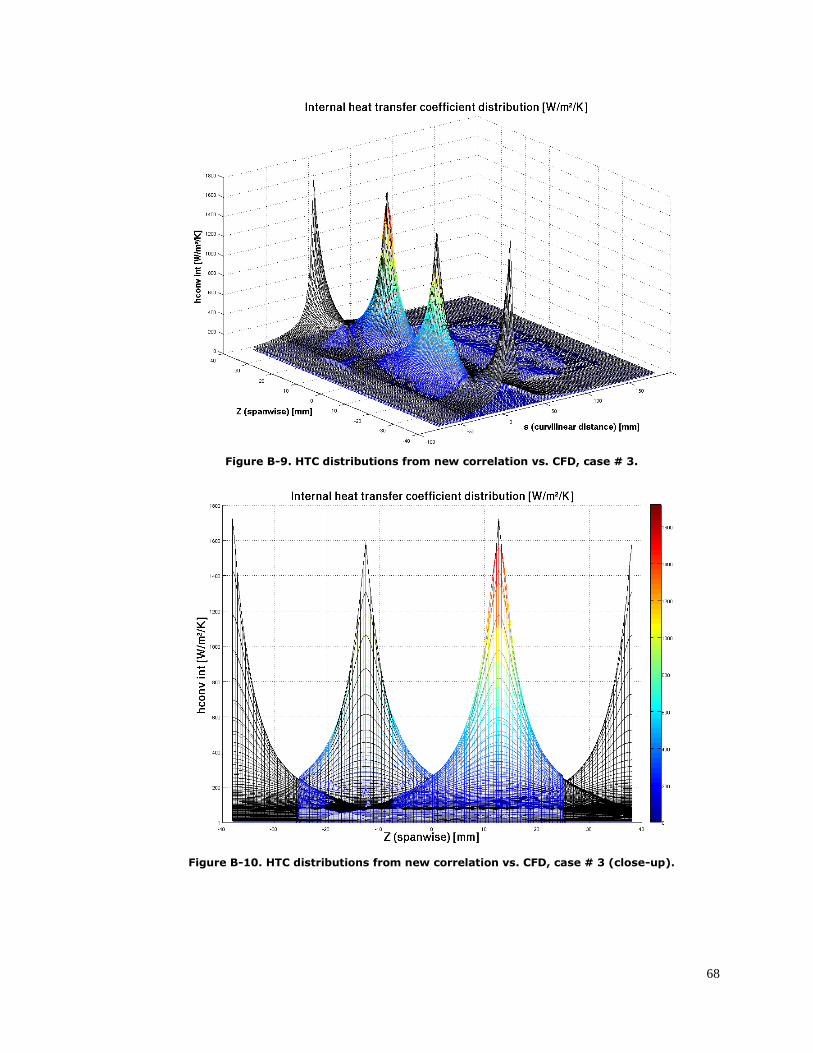
68
Figure B-9. HTC distributions from new correlation vs. CFD, case # 3.
Figure B-10. HTC distributions from new correlation vs. CFD, case # 3 (close-up).
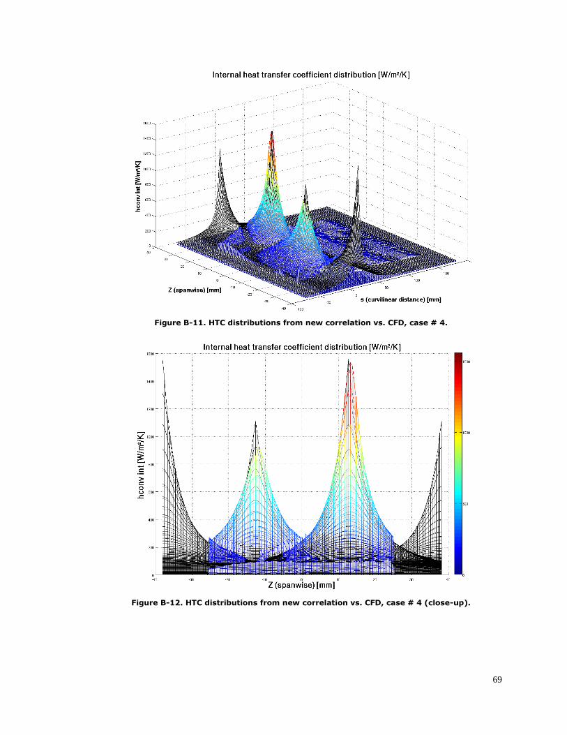
69
Figure B-11. HTC distributions from new correlation vs. CFD, case # 4.
Figure B-12. HTC distributions from new correlation vs. CFD, case # 4 (close-up).

70
Figure B-13. HTC distributions from new correlation vs. CFD, case # 5.
Figure B-14. HTC distributions from new correlation vs. CFD, case # 5 (close-up).
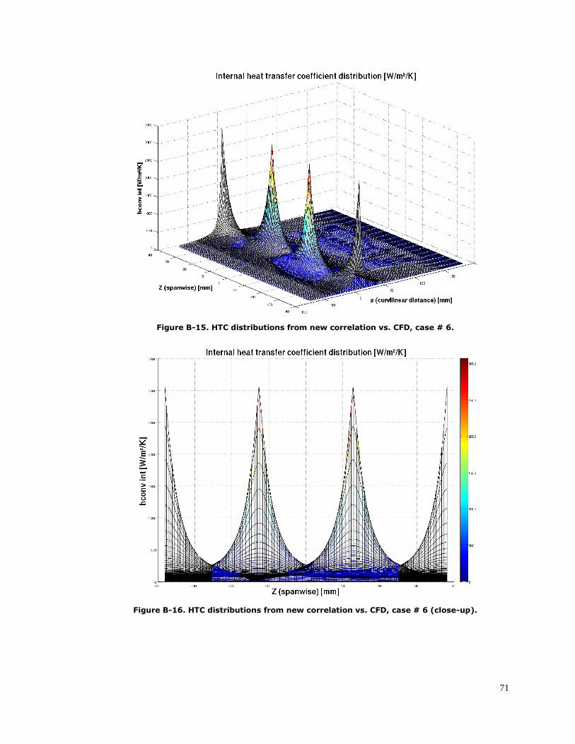
71
Figure B-15. HTC distributions from new correlation vs. CFD, case # 6.
Figure B-16. HTC distributions from new correlation vs. CFD, case # 6 (close-up).

72
Figure B-17. HTC distributions from new correlation vs. CFD, case # 7.
Figure B-18. HTC distributions from new correlation vs. CFD, case # 7 (close-up).

73
Figure B-19. HTC distributions from new correlation vs. CFD, case # 8.
Figure B-20. HTC distributions from new correlation vs. CFD, case # 8 (close-up).

74
APPENDIX C
C. APPROXIMATION OF WATER RUNBACK SOLUTION USING POD
To give a sense of the accuracy of the POD model, the following results taken from
the optimization procedure are presented. The solution computed directly from the
water film model (shown in colors) is compared to the corresponding solution
computed using the POD model (superimposed in black) for the same geometric
configuration. The water runback mass flow rate surface distribution and the wall
temperature distribution results are presented for three, four and five design
variables.
In the case of three design variables, the results are very satisfactory. In the
example shown in Figure C-1 and Figure C-2, the error for the water runback is
included within -6.1% and +2.9%, and concerning the wall temperature, the error is
within -1% and +0.8%, as shown in Figure C-3 and Figure C-4. More generally, the
level of error for the water runback is evaluated about ±5% and about ±1% for the
wall temperature. However, concerning water runback, the error at the relevant
locations (meaning the upper and lower ends of the protected surface) is contained
within ±3%.
In the case of four design variables, the results are still satisfactory even though the
error ranges are slightly higher than in the previous case. In the example shown in
Figure C-5 and Figure C-6, the error for the water runback is within -11.5% and
+8.5%, and concerning the wall temperature, the error is included within -2.2% and
+1.5%, as shown in Figure C-7 and Figure C-8. More generally, the level of error for
the water runback is evaluated at about ±10% and about ±2% for the wall
temperature. However, concerning water runback, the error at the relevant locations
is contained within ±5%.
In the case of five design variables, the interpolation method seems to have more
difficulties but the results are still satisfactory. In the example shown in Figure C-9
and Figure C-10, the error for the water runback is included within -21.1% and
+25.2%, and concerning the wall temperature, the error is included within -3.8%
and +4.9%, as shown in Figure C-11 and Figure C-12. More generally, the level of
error for the water runback is evaluated about ±20% and for the wall temperature
about ±5% (for five design variables). However, concerning water runback, the error
at the relevant locations is contained within ±10%.
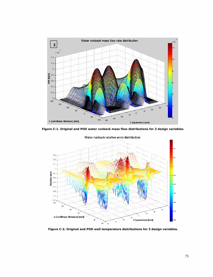
75
33
Figure C-1. Original and POD water runback mass flow distributions for 3 design variables.
Figure C-2. Original and POD wall temperature distributions for 3 design variables.
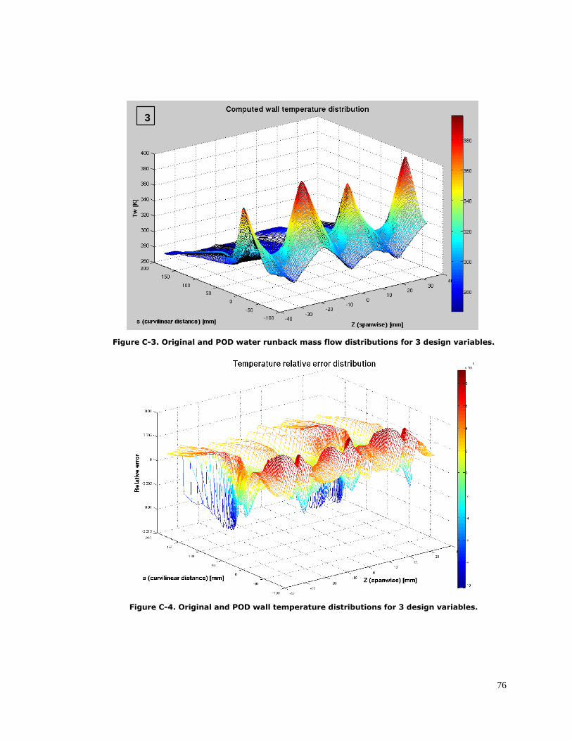
76
33
Figure C-3. Original and POD water runback mass flow distributions for 3 design variables.
Figure C-4. Original and POD wall temperature distributions for 3 design variables.

77
44
Figure C-5. Original and POD water runback mass flow distributions for 4 design variables.
Figure C-6. Original and POD wall temperature distributions for 4 design variables.

78
44
Figure C-7. Original and POD water runback mass flow distributions for 4 design variables.
Figure C-8. Original and POD wall temperature distributions for 4 design variables.

79
55
Figure C-9. Original and POD water runback mass flow distributions for 5 design variables.
Figure C-10. Original and POD wall temperature distributions for 5 design variables.

80
55
Figure C-11. Original and POD water runback mass flow distributions for 5 design variables.
Figure C-12. Original and POD wall temperature distributions for 5 design variables.
This reveals to some extent some limitations of using a reduced order model. The
introduced error might mislead the optimizer towards an “artificial” optimum since
the water runback solutions are slightly biased and therefore do not correspond
exactly to the associated geometric configurations, i.e. to the associated set of
design variables. Nevertheless, these results are very encouraging since the error

81
ranges are quite small and there is room for improvement with respect to the
interpolation method and the ROM.

82
APPENDIX D
D. DIRECT OPTIMIZATION VERSUS SEQUENTIAL OPTIMIZATION
The difference between direct and sequential optimization is easier to visualize with a
lower-dimension analogy in the case of a relatively simple arbitrarily chosen objective
function, like the following 2D optimization example. The objective function contains
a local minimum and a global minimum in order to use this example as a proof of
concept and explain the genetic algorithm optimization process for both direct and
sequential optimization.
D.1. Direct Optimization
Figure D-1. 2D optimization example via direct optimization.
The 2D optimization example presented in Figure D-1 is implemented into the genetic
algorithm module for a population size of 23 for 12 generations, with proportional
fitness scaling, tournament selection method, a single point cross-over fraction of
80% and an elite count of two.
The population is initially uniformly spread over the two-design-variable design
space, then the genetic algorithm process unfolds, gradually contracting the
population towards the global minimum until complete convergence, as shown in
Figure D-2.
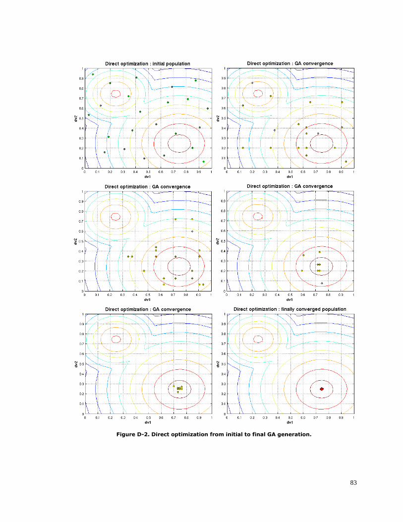
83
Figure D-2. Direct optimization from initial to final GA generation.
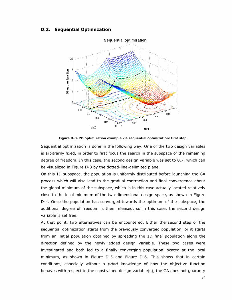
84
D.2. Sequential Optimization
Figure D-3. 2D optimization example via sequential optimization: first step.
Sequential optimization is done in the following way. One of the two design variables
is arbitrarily fixed, in order to first focus the search in the subspace of the remaining
degree of freedom. In this case, the second design variable was set to 0.7, which can
be visualized in Figure D-3 by the dotted-line-delimited plane.
On this 1D subspace, the population is uniformly distributed before launching the GA
process which will also lead to the gradual contraction and final convergence about
the global minimum of the subspace, which is in this case actually located relatively
close to the local minimum of the two-dimensional design space, as shown in Figure
D-4. Once the population has converged towards the optimum of the subspace, the
additional degree of freedom is then released, so in this case, the second design
variable is set free.
At that point, two alternatives can be encountered. Either the second step of the
sequential optimization starts from the previously converged population, or it starts
from an initial population obtained by spreading the 1D final population along the
direction defined by the newly added design variable. These two cases were
investigated and both led to a finally converging population located at the local
minimum, as shown in Figure D-5 and Figure D-6. This shows that in certain
conditions, especially without a priori knowledge of how the objective function
behaves with respect to the constrained design variable(s), the GA does not guaranty

85
completely avoiding converging towards a local extremum. Thankfully, it turns out
that there are two types of remedy for this kind of behavior. The first one is
mutation. Indeed, raising the mutation fraction from 20% to 75% in the first case
and to 60% in the second case led to final converged population at the global
minimum in both cases. However, this was done at the cost of more laborious
convergence which would necessitate more than twice the number of generations
(7+22 generations in the first case, 7+17 generations in the second case, as
opposed to 12 for direct optimization). The second remedy is to use a less converged
population from the 1D process, also spread along the direction defined by the newly
added design variable, with a slightly higher mutation fraction (30% instead of 20%).
This time, convergence towards the global minimum was achieved in 5+13
generations (cf. Figure D-7).
Figure D-4. Sequential optimization step 1: from initial to final GA generation.
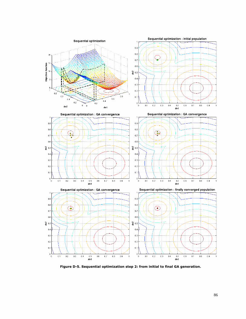
86
Figure D-5. Sequential optimization step 2: from initial to final GA generation.
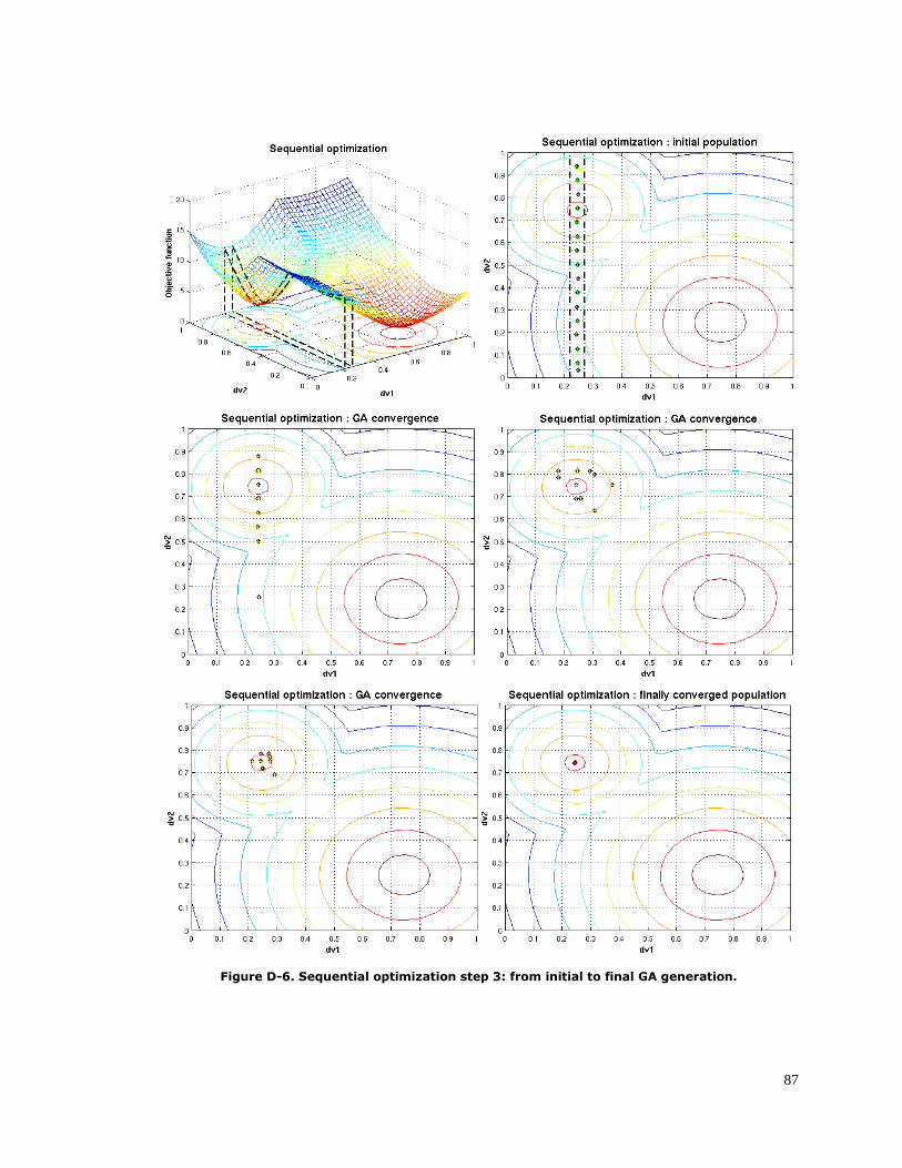
87
Figure D-6. Sequential optimization step 3: from initial to final GA generation.
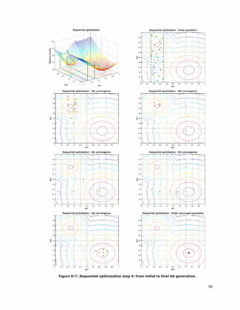
88
Figure D-7. Sequential optimization step 4: from initial to final GA generation.

89
From this simple example, it is quite obvious that when proceeding with sequential
optimization, the optimal configuration of the subspace might only be a local
optimum of the higher-dimension space. It is actually the most probable case since
the subspace is constrained arbitrarily with respect to the remaining design variables.
Therefore, starting from the lower-dimension optimal GA population results (even if it
is uniformly spread in the supplementary dimension(s)) would not necessarily lead to
significant improvement since it would introduce a bias in the GA initial population. It
would moreover result in a more laborious convergence, since it would require a
higher rate of mutation to recover the necessary diversity in the population.
Therefore, it would be more consistent and efficient to proceed with direct
optimization, except in the case where a priori knowledge about the choice of the
constrained design variables was available.
In any case, there is a compromise between accuracy and computational cost since
increasing the population size will help the exploration of the design space and
increase the consistency of the model, while increasing the number of generations
will improve the convergence level and the consistency and repeatability of the
results, at least as far as the genetic algorithm is concerned, but certainly at the cost
of additional computations.