www.CAEAI.com

A Guide to Random Data Analysis for Computational Fluid Dyanamics

A Guide to Random Data Analysis for Computational Fluid Dynamics

Copyright © 2016

Published by Computer Aided Engineering Associates Inc.

All rights reserved. Except as permitted under U.S. Copyright Act of 1976, no part ofthis publication may be reproduced, distributed, or transmitted in any form or by anymeans, or stored in a database or retrieval system, without the prior written permissionof the publisher.

Visit our website at www.caeai.com.

www.CAEA

I.co

m

A Guide to Finite Element Analysis of Par t-to - Par t Connec tions / 2

4

www.CAEA

I.co

m

A Guide to Random D ata Analysis for Computational Fluid D ynamic s / 3

Table of Contents

Chapter 1

Introduction

Techniques for Transient Flow Field Data 6

Chapter 2Introduction to The Fast Fourier Transform 10

Chapter 3Understanding The Fast Fourier Transform Inputs 14

Chapter 4Application of The Fast Fourier Transform 17

Chapter 5Accuracy of Your FFT and Parseval’s Theorem 20

Chapter 6The Short-Time Fourier Transform 22

Chapter 7Cross-Coherence 25

Chapter 8Auto and Cross Correlation 27

Chapter 9Two-Point Statistics 30

Chapter 10About CAE Associates 33

www.CAEA

I.co

m

The growth of industrial computing capacity has allowed for increased turbulence-resolving Computational Fluid Dynamics (CFD) approaches. As such, this has directly led to the need to resolve finer scale turbulence which in turn requires decreasing time steps. This increases run times and will result in larger data sets for post-processing. Today’s CFD engineers will increasingly find themselves in situations where they need to integrate reliable statistical measures into their everyday post-processing routines. If done properly, this will assure not only the quality of the post-processed data, but it will also allow the engineer to extract more information from their data that may be other-wise difficult to see.

At the beginning of a transient CFD analysis, the flow field is typically assigned an ar-bitrary initial condition or steady state solution. This solution must be advanced to a fully-developed statistically stationary state before meaningful sampling can begin. This guide aims to discuss two primary topics. The first of which is often times misun-derstood and is referred to as the “initial transients” in a CFD simulation and judging whether or not the flow field has advanced beyond this stage. The length of this initial transient is strongly case specific and is usually judged by intuitive inspection alone. Often times, we simply look for repeating, oscillating signals at various points in the flow fields which may not be adequate. Post-processing statistical laden results which are still in this window may be misleading. The second topic relates to the post-processing of transient data-sets and some of the more common techniques used for extracting the most from your data.

A Guide to Random D ata Analysis for Computational Fluid D ynamic s / 4

Introduction

www.CAEA

I.co

m

As stated previously, the amount of useful data embedded in a transient signal can be difficult to see for entry level and, often times, even advanced users. As such, this guide is intended to serve as a point of reference to aid the everyday CFD engineer when post-processing transient flow field data. It focuses on the introduction and application of only a few of the commonly used mathematical approaches that may be useful for in-terpreting transient data. The focus of this manual leans towards techniques which make use of transforming a time series data-set into the frequency domain for further analysis.

A Guide to Random D ata Analysis for Computational Fluid D ynamic s / 5

Introduction

www.CAEA

I.co

m

This chapter will discuss some of the post-proccessing techniques to consider when your CFD analysis is transient in nature. We will first need to gain an understanding of the concept of a stochastic process which is by definition a random process. A stochas-tic process is said to be ergodic if its statistical properties can be derived from only a subset of the entire dataset. This subset, or window of data, must represent the average statistical properties of the entire process regardless of where the window was extract-ed from in the process. In a nutshell, this implies that we expect that the statistics of the signal would converge to a single value if given a large enough sampling window. With Reynolds Averaged Navier-Stokes (RANS) CFD simulations, we most commonly focus on the first three statistical moments: the mean, variance, and standard-deviation. For advanced turbulence modeling with data acquired by the use of LES and DNS solvers, we may also decide to include skew and kurtosis in our random data analysis.

For illustration purposes, let’s consider a random pressure signal as shown in Figure 1. The data was acquired at a single point in space and sampled at uniform frequency of 100,000 [hz].

A Guide to Random D ata Analysis for Computational Fluid D ynamic s / 6

Chapter 1: Techniques for TransientFlow Field Data

Figure 1: Acquired random pressure signal

www.CAEA

I.co

m

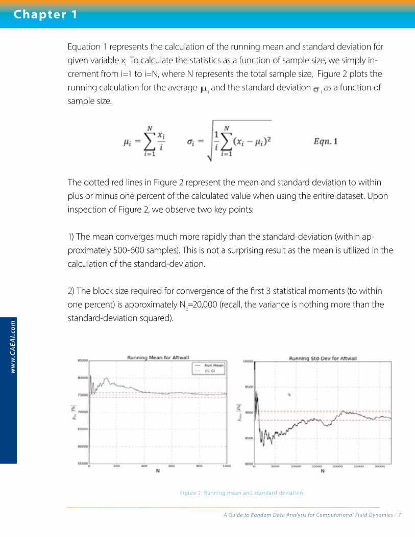
Equation 1 represents the calculation of the running mean and standard deviation for given variable xi. To calculate the statistics as a function of sample size, we simply in-crement from i=1 to i=N, where N represents the total sample size, Figure 2 plots the running calculation for the average i and the standard deviation i as a function of sample size.

The dotted red lines in Figure 2 represent the mean and standard deviation to within plus or minus one percent of the calculated value when using the entire dataset. Upon inspection of Figure 2, we observe two key points: 1) The mean converges much more rapidly than the standard-deviation (within ap-proximately 500-600 samples). This is not a surprising result as the mean is utilized in the calculation of the standard-deviation.

2) The block size required for convergence of the first 3 statistical moments (to within one percent) is approximately Nc=20,000 (recall, the variance is nothing more than the standard-deviation squared).

A Guide to Random D ata Analysis for Computational Fluid D ynamic s / 7

Figure 2: Running mean and standard deviat ion

Chapter 1

This implies we would require approximately of simulation time per block for our mean and variance to be fully converged to within one percent.

For transient analysis, which is expected to be stationary and ergodic, this simple anal-ysis can be quite powerful. The only way to ensure the initial transients have settled in your time marching simulation is by monitoring these statistics and ensuring they have converged to within a reasonable tolerance. If one wishes to only post-process mean flow field results from the transient data set - such as velocity and pressure quantities, the required amount of simulation effort is far less demanding than acquiring statistics related to the fluctuating components; (as they relate to the higher order statistical moments) such as turbulent velocities, Reynolds stress, or block sizes used for Fast Fou-rier Transform (FFT) analyses.

In the example above, we have only included the results from a single point in the flow field. Using ANSYS CFX, you can monitor these results using the transient-statistics tab and the “Output Control” menu which writes the running mean and standard deviation for the entire computational domain as illustrated in Figure 3 and 4 for flow over a cylinder. Using CFD-Post and its ability to compare-cases (say, at iteration “i” compared to iteration “i+1000”), you could generate contour plots and monitor these statistics for multiple planes. This would allow you to rapidly gain a qualitative assess-ment of global transient-statistical convergence levels.

www.CAEA

I.co

m

A Guide to Random D ata Analysis for Computational Fluid D ynamic s / 8

Chapter 1

Figure 3: Instantaneous u-velocit y contours for f low over a c yl inder s tar ted f rom 0 velocit y

This chapter illustrated how you could apply random data analysis statistical tech-niques to monitor the convergence levels related to the initial transients for your time marching analysis. As we have seen, when post processing transient CFD data, there are multiple items to consider. We must consider how well the solver converges on an iteration by iteration basis and how far the simulation has been carried out. We also have found we need to monitor the flow field statistics to assess whether or not the converged transient solution is completely reliable and producing meaningful results. In Chapter 2, the Fast Fourier Transform and its implementation will be discussed.

www.CAEA

I.co

m

A Guide to Random D ata Analysis for Computational Fluid D ynamic s / 9

Chapter 1

Figure 4: Mean u-velocit y contours for f low over a c yl inder s tar ted f rom 0 velocit y

www.CAEA

I.co

m

In Chapter 1, the concept of a stochastic process and random data analysis were dis-cussed. Specifically, the focus was on computing temporal statistics such as the mean and standard deviation. In this chapter, the Fast Fourier Transform (FFT) and its imple-mentation and use in data post-processing of CFD analyses will be discussed. The French mathematician J. B. J. Fourier discovered that periodic waveforms can be modeled as the sum of sine and cosine waves called a Fourier series. The mathematical expression is given in Equation 1 for a generic signal with a known range. Application of Equation 1 for a square wave with increasing values of “n” yields Figure 1, where it is ap-parent that as n -> ∞ the square wave is more accurately reproduced.

A Guide to Random D ata Analysis for Computational Fluid D ynamic s / 10

Chapter 2: Introduction to The Fast Fourier Transform

Figure 1: Par t ial sums of the Fourier ser ies of a square wave (ht tp: //w w w.reed.edu/physics/courses/Physics331. f08/pdf/Fourier.pdf )

The Fourier transform is used to represent a periodic function by a discrete sum of com-plex exponentials. Instead of Equation 1 above, we could equally write the summation in complex form:

If we define a new variable k=2πn⁄α we can define the Fourier integral (after some math)

If we want a result for F(k), which is called the Fourier transform of f(x), we apply equation 2 in the limit as approaches infinity with the Fourier series coefficients

The Fourier transform is closely related to a Fourier series and is used to represent a general function by a continuous superposition (or integral) of complex exponentials. The Fourier transform decomposes an arbitrary waveform into its sine components, thus revealing its frequency content that might else be difficult to detect. A Discrete-Time Fourier transform (DTFT) is a form of the Fourier transform that is applicable to uniformly sampled continuous functions. The Fast Fourier Transform (FFT) takes ad-vantage of powers of two and is a numerically efficient implementation of computing DTFTs. Simply stated, the FFT is an efficient numerical algorithm that allows for the transformation of a time dependent signal into the frequency domain (or vice-versa).

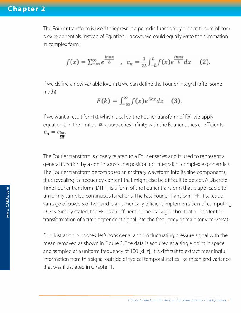
For illustration purposes, let’s consider a random fluctuating pressure signal with the mean removed as shown in Figure 2. The data is acquired at a single point in space and sampled at a uniform frequency of 100 [kHz]. It is difficult to extract meaningful information from this signal outside of typical temporal statics like mean and variance that was illustrated in Chapter 1.

www.CAEA

I.co

m

A Guide to Random D ata Analysis for Computational Fluid D ynamic s / 11

Chapter 2

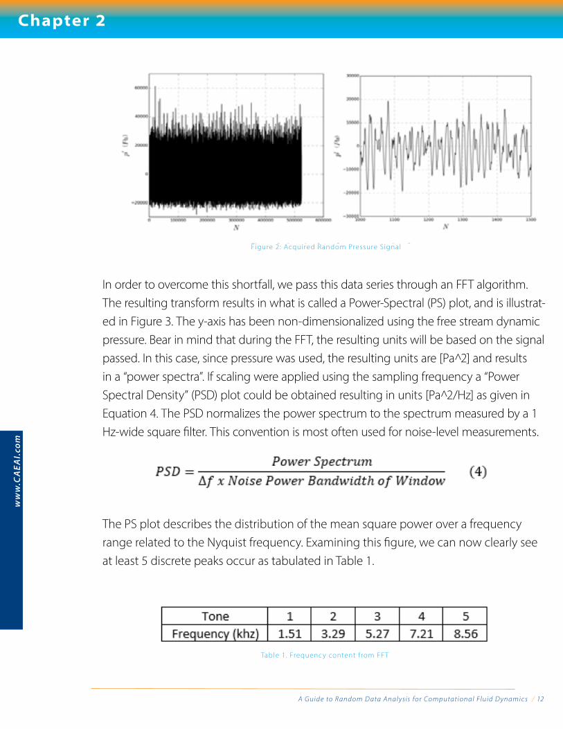
In order to overcome this shortfall, we pass this data series through an FFT algorithm. The resulting transform results in what is called a Power-Spectral (PS) plot, and is illustrat-ed in Figure 3. The y-axis has been non-dimensionalized using the free stream dynamic pressure. Bear in mind that during the FFT, the resulting units will be based on the signal passed. In this case, since pressure was used, the resulting units are [Pa 2̂] and results in a “power spectra”. If scaling were applied using the sampling frequency a “Power Spectral Density” (PSD) plot could be obtained resulting in units [Pa 2̂/Hz] as given in Equation 4. The PSD normalizes the power spectrum to the spectrum measured by a 1 Hz-wide square filter. This convention is most often used for noise-level measurements.

The PS plot describes the distribution of the mean square power over a frequency range related to the Nyquist frequency. Examining this figure, we can now clearly see at least 5 discrete peaks occur as tabulated in Table 1.

www.CAEA

I.co

m

A Guide to Random D ata Analysis for Computational Fluid D ynamic s / 12

Chapter 2

Figure 2: Acquired Random Pressure Signal

Table 1. Frequenc y content f rom FF T

Further, it is clear that the third tone is dominant and exhibits over three times the peak power compared to the other tones. The total power could be determined by obtaining the area under the curve with specified frequency intervals if desired such as done with Octave analysis.

In Chapter 3, Fast Fourier Transform Inputs will be explored in greater detail.

www.CAEA

I.co

m

A Guide to Random D ata Analysis for Computational Fluid D ynamic s / 13

Chapter 2

Figure 2: Acquired Random Pressure Signal

Figure 3: FF T of the Pressure Signal

www.CAEA

I.co

m

This chapter will take a more in-depth look at the inputs required for the FFT and will help the CFD engineer understand how to utilize it properly. To do this, the focus will be on a built in function in Python (Anaconda) to generate the FFT’s using Welch’s method. Below is the function call used and the inputs will be discussed systematically.

Pxx,f = mpl.psd(pfluc,nfft,fs,window=mlab.window_hanning,scale_by_freq=False,sides=’onesided’,noverlap=nlap)

The FFT Command Line and Welch’s Method:

Welch’s method is based on the concept of decomposing the acquired signal into segments, performing the FFT on individual blocks, and taking the resulting ensem-ble-average of the constructed periodograms. Welch’s method may be considered an improvement on the standard spectrum methods, as it reduces the noise in the estimated power spectra. The drawback is that it does this by reducing the frequency resolution (as nfft is smaller than N).

A Guide to Random D ata Analysis for Computational Fluid D ynamic s / 14

Chapter 3: Understanding The Fast Fourier Transform Inputs

Figure 1: Welch’s Method for FF T with No Overlapping

Frequency Resolution:IFrequency resolution is illustrated by Equation 1. In order to increase the frequency resolution (i.e. reduce Δf ), the ensemble period (T) must be increased. This is achieved by either reducing the sampling frequency (fs), or increasing the number of sampling points per ensemble (nfft).

pfluc:This is the signal passed to the FFT that is assumed to be discretely sampled with a uniform sampling frequency. The mean has been removed from the signal resulting in just the fluctuating component of the variable.

nfft:For FFT’s, the signal will be decomposed into powers of nfft = 2m where “m” is speci-fied by the user. Trailing data points after the last block is created are simply truncated.

Window:Applying a “Window” to an FFT in essence modulates the input signal so that the spec-tral leakage is evened out. If we take a sine wave, you would expect to see just one sample at the frequency of the signal. Spectral leakage occurs due to the fact we are “binning” the data and sometimes the frequency calculated falls right at the edge of our bins. The power from the sample may leak out to the surrounding frequency bins, and is thus referred to as spectral leakage. Windowing reduces the amplitude of the samples at the beginning and end of the window and alters this leakage. Windowing is implemented by multiplying the input signal with a windowing function. There are many common windowing functions, but for CFD and turbulent flows, the Hanning window is the most widely adopted. The Hanning window is given by:

www.CAEA

I.co

m

A Guide to Random D ata Analysis for Computational Fluid D ynamic s / 15

Chapter 3

Scaling:Scaling by frequency specifies whether the resulting spectral density values should be scaled by the scaling frequency, which gives density in units of This allows for integration over the returned frequency values. Commonly, PSD’s are reported in terms of decibels in which case the PSD must be scaled using:

where THH represents the Threshold of Human Hearing typically taken as 2e-05 [Pa].

One or Two-Sided:Specifies which side (or both) of the spectrum to be returned.

Overlapping:Overlapping your data is a method to ensure you get the highest number of Nblocks increasing your averaging accuracy and frequency resolution by using repetitive data. As shown in Figure 2, we are in essence sliding our nfft segment back to the left reuti-lizing a defined percentage of overlap points.

Now that we have a background on the FFT implementation in codes like Python, we can exercise the code and discuss the results. This will be the focus of Chapter 4.

www.CAEA

I.co

m

A Guide to Random D ata Analysis for Computational Fluid D ynamic s / 16

Chapter 3

Figure 2: I l lustrat ion of 50% Overlapping

www.CAEA

I.co

m

With a firm understanding of the required inputs for performing a FFT analysis, we are ready to execute the algorithm for a representative data set and discuss the effects of the chosen parameters. This chapter will focus on the built in function in Python (Ana-conda) to generate the FFT’s using Welch’s method as discussed in the previous chap-ters and repeated below for clarity.

Pxx,f=mpl.psd(pfluc,nfft,fs,window=mlab.window_hanning,scale_by_freq=False,sides=’onesided’,noverlap=nlap).

Selection of nfft:Based on the frequency resolution given by Equation 1, it is easy to see that the larger the size of your nfft, the more accurate your frequency resolution becomes for a fixed sampling rate.

Unfortunately, by increasing your nfft you lower the number of available periodo-grams used in the averaging of the final FFT, as each window has now been extended. To mitigate this, you can use overlapping. Typically, the optimal overlap percentage is between 50 and 75% of the nfft size. Ultimately, the choice of nfft becomes a balanc-ing act between the desired accuracy of the frequency resolution vs. the magnitude of the spectra.

Let’s assume we have a a scenario where the lowest known resonate frequency is near 1 [kHz] . Let’s further assume we have the capability for infinite sampling frequency.

A Guide to Random D ata Analysis for Computational Fluid D ynamic s / 17

Chapter 4: Application of The Fast Fourier Transform

In this scenario, the lowest frequencies are the most demanding to capture because they require they longest sampling times. For this scenario, let’s take the sampling fre-quency to be fixed at 1e-05 [s] or (100 [kHz]) with N=219 total points. We desire at least 20 cycles per nfft period to ensure statistical accuracy (the more the better, of course). This means we would need at least 0.05 [s] of simulation time and 5,000 points per nfft. We have now given ourselves a reasonable estimate for our selection of nfft that should be between 212 and 213. The trade-off here is with the accuracy of the resulting frequency resolution as seen in Table 1. But, we also want to average multiple periodo-grams (per Welch’s method) to ensure accuracy. Thus, we may want on the order of 30 ensembles which requires at least a total signal length of N=150,000 points. Remember, we are using powers of 2 so we really need the next power of 2, which would be 218.

Table 1 illustrates our corresponding frequency resolution (bin width), number of aver-aged periodograms, and the number of shedding cycles per period for selected values of nfft.

The following figures were generated using the FFT call presented at the beginning of this chapter with a Hanning window and no overlapping. Figure 1 illustrates the effect of the selection of nfft on your FFT.

www.CAEA

I.co

m

A Guide to Random D ata Analysis for Computational Fluid D ynamic s / 18

Chapter 4

Figure 1: FF T Based on Selec ted Sizesfor nf f t

Figure 2 illustrates the effect of the selection of frequency resolution on your resulting FFT. The original signal length was decimated by a factor of 2 and 4 to emulate larger sampling frequencies. Similar to Figure 1, the peak values decrease and the broadening of the peaks is still evident as the frequency resolution increases. This brings to light that when comparing spectral plots with data obtained from ex-perimental or numerical methods, care must be taken to understand exactly how the plots were constructed. (Not just the physics of the problem!) It is important that the spectral plots be constructed in the same fashion. If complete information is not sup-plied on how the FFT was performed, one may end up with misleading discrepancies when comparing back to back figures!

Now that the background, required inputs, and execution of a typical FFT algorithm have been presented, we need to address the accuracy of the computation. This will be the focus of Chapter 5.

www.CAEA

I.co

m

A Guide to Random D ata Analysis for Computational Fluid D ynamic s / 19

Chapter 4

Figure 2: FF T Based on Frequenc y Resolution Acquired by Decimating the Original Signal

www.CAEA

I.co

m

The previous chapter discussed some of the most common variables utilized when performing an FFT analysis. This chapter will discuss some key points when evaluating the accuracy of a computed FFT by discussing Nyquist’s criterion and Parseval’s theo-rem.

Nyquist Criterion:For a signal to be accurately reconstructed from a discrete set of sampled points, the sampling rate should be at minimum twice the maximum frequency of interest. Thus, the Nyquist frequency is defined as half of the sampling frequency of a discrete signal. The Nyquist rate is the minimum sampling rate that satisfies the Nyquist sampling criterion. If you wish to extract the frequency content from a 1 [kHz] signal, then the Nyquist criterion tells us that our minimum required sample rate is 500 [Hz]. The most straightforward way to avoid aliasing is to ensure your sampling frequency is high enough to capture the spatial and or temporal variations in a given signal.

Parseval’s Theorem:Parseval’s Theorem is a simple statement of the conservation of energy. The theorem states that the total energy computed in the time domain must equal the total en-ergy computed in the frequency domain. In other words, no loss of energy (or power) should occur during the transformation from one space into another. For a continuous integrable function, this is given by Equation 1below.

A Guide to Random D ata Analysis for Computational Fluid D ynamic s / 20

Chapter 5: Accuracy of Your FFT and Parseval’s Theorem

For discretely sampled data series, the relationship is simply the sums given by Equa-tion 2.

The following section focuses on the built in function(s) in Python (Anaconda) and the implementation of Parseval’s Theorem. The snippet of code is well commented so adaption to another engine of choice should be somewhat seamless.

m=13## Do FFT# pfluc is the acquired signal from a uniformly sampled time-historynfft = int(2**m) # size of each record to ensemble averagenlap = int(0) # No. of pts to overlapfr = fs / float(nfft) # Calculate frequency resolutionk = int((N-nlap)/(nfft-nlap)) # No. of periodograms to average# Get 2-sided FFT with appropiate scaling that yields [units^2/Hz]Pxx,f = mpl.psd(pfluc,nfft,fs,window=mlab.window_hanning,scale_by_freq=True,noverlap=nlap)parseval_side2 = (np.trapz(Pxx,f )/fs) # Num. int. PSD to get units [Pa^2]. Scale by fs for units matchingparseval_side1 = np.var(pfluc) # Get variance of time domain to get [Pa^2]Error = (np.abs(parseval_side1-parseval_side2)/parseval_side1)*100 # Compute error

Chapter 6 will discuss some of the shortcomings of the FFT and discuss other potential data that can be extracted from your time series.

www.CAEA

I.co

m

A Guide to Random D ata Analysis for Computational Fluid D ynamic s / 21

Chapter 5

www.CAEA

I.co

m

There are many inherent shortcomings of an FFT analysis that the CFD engineer may need to be aware of, along with the potential work arounds. When performing an FFT analysis, you can switch to and from the frequency domain revealing frequency con-tent and amplitude information with ease. One drawback is there is no information provided for the time history of a given amplitude or peak. One of the most obvious questions one may ask is: “is my dominant amplitude apparent for all time or does it reveal itself only intermittently?” When the peak with the dominant amplitude switch-es frequencies as a function of time, the signal is said to exhibit “mode-switching.” Joint Time-Frequency Analysis (commonly referred to as Short-Time Fourier Trans-forms, or STFT) using Fourier transforms, given by Equation 1, provides information containing frequency, time, and amplitude allowing one to visualize the time-evolu-tion of the frequency content.

The spectrograms for this approach are computed using a short time duration where z(t) is an applied window function. The time dependent input signal is partitioned into several disjointed or overlapped blocks by multiplying the signal with a specified win-dow. The FFT is then applied to each block. The blocks occupy different time periods so the resulting STFT computes the spectral content of the input signal at each period. The STFT therefore represents the time-dependent power spectrum of the input sig-nal. The steps for computing the STFT are as follows:

1. Choose a window function of finite length2. Place the window on top of the signal at t = 0 [s]3. Truncate the signal using this window

A Guide to Random D ata Analysis for Computational Fluid D ynamic s / 22

Chapter 6: The Short-Time Fourier Transform

4. Compute the FFT of the truncated signal5. Incrementally slide the window to the right6. Repeat steps 3-5 until the end of the signal is reached

The resulting spectrogram (where the magnitude has been normalized) for the sig-nal used in this series is provided in Figure 1(c) below. Bear in mind, that due to the uncertainty principle discussed above, a wide window will result in good frequency resolution, but poor time resolution. Conversely, a narrow window will yield better time resolution at the expense of frequency resolution. Four discrete tones are still apparent (where the 5th tone and beyond are masked by the color scheme as their magnitudes are on the order of the broadband noise) and we can now see their magnitude as a function of time. It is apparent that tone three is dominant for most of the time history but there are periods in time where this signal drops out (between 0.15 and 0.20 [s] for example) suggesting that mild mode switching may be apparent.

www.CAEA

I.co

m

A Guide to Random D ata Analysis for Computational Fluid D ynamic s / 23

Chapter 6

Figure 1: I l lustrat ion of the Uniform-ly Sampled Raw Signal , the Corre -

sponding FF T and the STF T.

A well-known property of the Fourier transform pair s(t) and s(ω) is the uncertainty principle which states the time duration (∆t) of s(t) and the frequency bandwidth (∆ω) are related by ∆t ∆ω≥1/2. This implies a longer time duration of the input signal will re-sult in a smaller frequency bandwidth. Conversely, the larger the frequency bandwidth of the transformed input signal, results in a shorter duration of the input signal. This illustrates the tradeoff between the frequency resolution and time resolution when using this method. The precision of the transform is determined by the size of the se-lected window and is fixed for all frequencies.

A technique which allows the use of variable window sizes may be employed to over-come the time and frequency resolution tradeoff inherent with the STFT. This analysis is called Wavelet analysis and is a topic for future discussion. Chapter 7 will discuss another topic related to the FFT called Cross-Coherence analysis.

www.CAEA

I.co

m

A Guide to Random D ata Analysis for Computational Fluid D ynamic s / 24

Chapter 6

www.CAEA

I.co

m

This chapter introduces the concept of Cross-Coherence and discusses some benefits of performing this type of analysis.

So far, we have dealt with extracting information from a single time series. In this chapter, we will discuss a method for relating two time-dependent signals as a func-tion of frequency. This type of analysis is referred to as the level of “Coherence” be-tween the signals. The Cross-Coherence of two-such signals is given by Equation 1 where φyx (f) represents the cross-spectra of the two signals and is normalized by the square root of each signal’s respective auto-spectra.

If the signals are identical, the correlation coefficient is unity, and if they are unrelated the correlation coefficient is zero. If the signals are identical, but the phase is shifted by exactly 180 degrees, then the correlation coefficient is -1.

A Guide to Random D ata Analysis for Computational Fluid D ynamic s / 25

Chapter 7: Cross- Coherence

Figure 1: Cross- Coherence of a Baseline Conf iguration amd a Geometr ical ly Modif ied Scenar io, Sampled at the Same Points in Space and Frequenc y. The FF T (at the same point) are Embedded in the Right Hand Corner

The coherence plot for the cases in the first subfrigure show a strong correlation with coefficients exceeding 0.80 for most peak tones. Since the pressure signal is being cor-related, this tells us that the pressure at the aft-sensing point is strongly correlated with what is happening as you progress away from that point (as x/L decreases). Conversely, for the altered case, the magnitudes of the coherence fall significantly, coinciding with a broadening and lowering of the peaks presented on the embedded FFT spectra. This suggests that the feedback mechanism thought to be responsible for generating these peaks has been disturbed.

The use of Cross-Coherence plots is yet another method for extracting useful informa-tion from your time series data, but their use requires at least two data sets with the same sampling rate, equivalent length, and sampling period. Chapter 8 will explain both auto and cross-correlation in detail.

www.CAEA

I.co

m

A Guide to Random D ata Analysis for Computational Fluid D ynamic s / 26

Chapter 7

www.CAEA

I.co

m

The use of Short-Time Fourier to obtain amplitude, time, and frequency content was discussed in Chapter 7. This chapter introduces the concept of Cross-Correlation and we will discuss some benefits of performing this type of analysis.

Cross-Correlation analysis can be used to help determine how strongly two signals in the time-domain are related. If the signals are identical the correlation coefficient is unity and if they are unrelated the correlation coefficient is zero. If the signals are identical except that the phase is shifted by exactly 180 degrees then the correlation coefficient is -1. When two independent signals are compared in the time domain the procedure is known as cross-correlation. Autocorrelation is a special case of cross-correlation where the same signal is compared to itself. The autocorrelation coefficient of a signal x(t) is given as:

The time lag, or separation between points, is given r∆t. The maximum number of lags is given by r. The cross-correlation of two signals x(t) is and y(t) is then given by Equa-tion 2.

A Guide to Random D ata Analysis for Computational Fluid D ynamic s / 27

Chapter 8: Auto and Cross Correlation

The cross-correlation performed in the time domain is a computationally inefficient approach which may be computed faster taking advantage of the FFT. The enhanced correlation is written by convolving the first function, g(t), with the time-reverse of the second function given by h(t) in Equation 3:

where the * is the complex conjugate and the x indicates the cross-correlation. This may be implemented with the following routine using Python:

def xcorrNorm( y, y2, fs, maxlags): import numpy as np ####### Cross Correlation via FFT ############### fs=float(fs) y = y - np.mean(y) # sig 1 y2 = y2 - np.mean(y2) # sig 2 N = len(y) sp = np.fft.rfft(y) # compute FFT transform of 1st signal sp2 = np.fft.rfft(y2) # compute FFT of 2nd sig sp = np.conj(sp) # complex conjugate of 2nd sig rho = np.fft.irfft( sp*sp2 ) # inverse transform of the convolution rho = np.fft.fftshift(rho) # shift fft so 0 is centered rho = rho / (np.std(y) * np.std(y2)) / N # normalize tlag = np.int32(np.linspace(-len(rho)/2,len(rho)/2,len(rho))) / fs # Get lags rho = rho[(N/2) - maxlags : (N/2) + maxlags] # extract maxlag data tlag = tlag[(N/2) - maxlags : (N/2) + maxlags] # extract maxlag data return tlag, rho

www.CAEA

I.co

m

A Guide to Random D ata Analysis for Computational Fluid D ynamic s / 28

Chapter 8

Figure 1 represents the cross and auto correlation of given pressure signals discussed in the previous blogs. Referring to Figure 1: since we know the offset from the leading edge to x/L=0.25 we may estimate the upstream speed of the propagating wave by looking at the offset of the corresponding peaks of these curves. In this example we

obtain (L=0.0762 [m]) and a velocity of

Also, analogous to comparing peaks for the cross-coherence in the previous chapter, we see here that the cross-correlations exhibit well-correlated peaks indicating what is sensed at the aft wall is also strongly correlated with the pressure signal sensed up-stream. As expected, the black line exhibits a peak of unity at zero lag since this is the auto-correlation. Chapter 9 will discuss the use of two point statistics using turbulent velocity and fluctuating pressures.

www.CAEA

I.co

m

A Guide to Random D ata Analysis for Computational Fluid D ynamic s / 29

Chapter 8

Figure 1: Auto and Cross Correlat ion for the T ime Ser ies Presented in Previous Chapters

www.CAEA

I.co

m

In the previous chapter, the use of auto and cross-correlations were discussed. These are commonly used to gain an understanding of the relationship between random signals. The final chapter in this guide discusses the use of two-point statistics using turbulent velocities or pressures.

Several statistical concepts can be used for the analysis of unsteady quantities of inter-est and in this chapter, I will focus on unsteady or fluctuating pressure signals. The fluctuating component of the pressure are found from a classical Reynolds decompo-sition. Equation 1 gives the fluctuating pressure where the prime represents the fluc-tuating component of the variable, the overbar represents the mean, and a variable with no demarcation represents the instantaneous value.

(1)

The mean takes the traditional definition given in Equation 2 below where the num-ber of independent observations is given by N, which is sufficiently large to ensure the mean value has converged.

(2)

The variation of the measured unsteady pressure is studied using the root-mean-square (rms) of the fluctuating variable and is commonly referred to as the standard deviation in statistical literature.

A Guide to Random D ata Analysis for Computational Fluid D ynamic s / 30

Chapter 9: Two-Point Statistics

(3)

The length scale variations in the shear layer are studied by employing a two point spatial cross-correlation on the components of the fluctuating pressure with an origin defined at some fixed point with a known separation . The two point spatial tensor is then given by:

(4)

At zero separation, if using velocity instead of pressure, the diagonal elements represent the normal turbulent velocities and the off diagonals would represent the turbulent shear stresses. With the spatial separation represented in the correlation, one may look at how the velocity at the defined origin is related to the velocity at another point which inherently defines a length of how far apart the selected variables are related.

Figure 1 (next page) illustrates spatial correlation plots of the fluctuating surface pres-sure as a function of separation with the origin located at the center point of the aft wall for each configuration, as introduced in previous chapters. The baseline case exhibits a much larger, highly correlated region that extends from just below the origin to the top of the aft wall. The controlled configuration’s well correlated region is noticeably more compact, which suggests that smaller scale structures have impacted the aft wall. This is consistent with the argument that the control is breaking up the organized turbulent features found in the upstream shear layer which ultimately impact the aft wall.

www.CAEA

I.co

m

A Guide to Random D ata Analysis for Computational Fluid D ynamic s / 31

Chapter 9

The controlled configuration’s well correlated region is noticeably more compact, which suggests that smaller scale structures have impacted the aft wall. This is consistent with the argument that the control is breaking up the organized turbulent features found in the upstream shear layer which ultimately impact the aft wall.

This chapter wraps up the guide on random data analysis techniques commonly used for CFD analysis.

www.CAEA

I.co

m

A Guide to Random D ata Analysis for Computational Fluid D ynamic s / 32

Chapter 9

Figure 1: Figure 1. Fluc tuating sur face pressure correlat ion on the af t wall with the or igin located at the center point .

www.CAEA

I.co

m

Since 1981, CAE Associates been helping companies large and small maximize value from engineering simulation through expert FEA consulting and CFD consulting ser-vices.

As an ANSYS channel partner since 1985, we provide full service technical support to over 100 companies in our region, including some of the world’s largest and sophisti-cated users of simulation like General Electric and United Technologies.

We offer a range of consulting options to fit unique and specialized needs of our clients. It could be as simple as getting to the bottom of a product failure, or as complex as developing the infrastructure and process for simulation within the entire organization using a combination of software, training, mentoring and automation.

Our team of senior technical specialists bring graduate-level educations and an average of 15 years of real-world experience in a variety of industries including: aerospace, elec-tronics, consumer product, turbomachinery, civil engineering, manufacturing, biomedi-cal, energy, and nuclear power.

For questions and to find out more about how CAE Associates can help you solve your engineering analysis challenges, please contact us at info@caeai.com.

A Guide to Random D ata Analysis for Computational Fluid D ynamic s / 33

Chapter 10: About CAE Associates Inc.