A Guide to Complex Variables
185
A Guide to Complex Variables Steven G. Krantz October 14, 2007
Transcript of A Guide to Complex Variables

A Guide to Complex Variables
Steven G. Krantz
October 14, 2007

iii
To Paul Painleve (1863–1933).

Table of Contents
Preface v
1 The Complex Plane 11.1 Complex Arithmetic . . . . . . . . . . . . . . . . . . . . . . . 1
1.1.1 The Real Numbers . . . . . . . . . . . . . . . . . . . . 11.1.2 The Complex Numbers . . . . . . . . . . . . . . . . . . 11.1.3 Complex Conjugate . . . . . . . . . . . . . . . . . . . . 21.1.4 Modulus of a Complex Number . . . . . . . . . . . . . 31.1.5 The Topology of the Complex Plane . . . . . . . . . . 31.1.6 The Complex Numbers as a Field . . . . . . . . . . . . 71.1.7 The Fundamental Theorem of Algebra . . . . . . . . . 8
1.2 The Exponential and Applications . . . . . . . . . . . . . . . . 81.2.1 The Exponential Function . . . . . . . . . . . . . . . . 81.2.2 The Exponential Using Power Series . . . . . . . . . . 91.2.3 Laws of Exponentiation . . . . . . . . . . . . . . . . . 91.2.4 Polar Form of a Complex Number . . . . . . . . . . . . 91.2.5 Roots of Complex Numbers . . . . . . . . . . . . . . . 111.2.6 The Argument of a Complex Number . . . . . . . . . . 131.2.7 Fundamental Inequalities . . . . . . . . . . . . . . . . . 13
1.3 Holomorphic Functions . . . . . . . . . . . . . . . . . . . . . . 141.3.1 Continuously Differentiable and Ck Functions . . . . . 141.3.2 The Cauchy-Riemann Equations . . . . . . . . . . . . . 141.3.3 Derivatives . . . . . . . . . . . . . . . . . . . . . . . . 151.3.4 Definition of Holomorphic Function . . . . . . . . . . . 161.3.5 The Complex Derivative . . . . . . . . . . . . . . . . . 171.3.6 Alternative Terminology for Holomorphic Functions . . 18
i
ii
1.4 Holomorphic and Harmonic Functions . . . . . . . . . . . . . . 191.4.1 Harmonic Functions . . . . . . . . . . . . . . . . . . . 191.4.2 How They are Related . . . . . . . . . . . . . . . . . . 19
2 Complex Line Integrals 212.1 Real and Complex Line Integrals . . . . . . . . . . . . . . . . 21
2.1.1 Curves . . . . . . . . . . . . . . . . . . . . . . . . . . . 212.1.2 Closed Curves . . . . . . . . . . . . . . . . . . . . . . . 222.1.3 Differentiable and Ck Curves . . . . . . . . . . . . . . 222.1.4 Integrals on Curves . . . . . . . . . . . . . . . . . . . . 232.1.5 The Fundamental Theorem of Calculus along Curves . 242.1.6 The Complex Line Integral . . . . . . . . . . . . . . . . 242.1.7 Properties of Integrals . . . . . . . . . . . . . . . . . . 25
2.2 Complex Differentiability and Conformality . . . . . . . . . . 262.2.1 Limits . . . . . . . . . . . . . . . . . . . . . . . . . . . 262.2.2 Continuity . . . . . . . . . . . . . . . . . . . . . . . . . 262.2.3 The Complex Derivative . . . . . . . . . . . . . . . . . 272.2.4 Holomorphicity and the Complex Derivative . . . . . . 272.2.5 Conformality . . . . . . . . . . . . . . . . . . . . . . . 28
2.3 The Cauchy Integral Formula and Theorem . . . . . . . . . . 292.3.1 The Cauchy Integral Theorem, Basic Form . . . . . . . 292.3.2 The Cauchy Integral Formula . . . . . . . . . . . . . . 292.3.3 More General Forms of the Cauchy Theorems . . . . . 302.3.4 Deformability of Curves . . . . . . . . . . . . . . . . . 31
2.4 The Limitations of the Cauchy Formula . . . . . . . . . . . . . 32
3 Applications of the Cauchy Theory 353.1 The Derivatives of a Holomorphic Function . . . . . . . . . . . 35
3.1.1 A Formula for the Derivative . . . . . . . . . . . . . . 353.1.2 The Cauchy Estimates . . . . . . . . . . . . . . . . . . 353.1.3 Entire Functions and Liouville’s Theorem . . . . . . . . 363.1.4 The Fundamental Theorem of Algebra . . . . . . . . . 373.1.5 Sequences of Holomorphic Functions and their Deriva-
tives . . . . . . . . . . . . . . . . . . . . . . . . . . . . 383.1.6 The Power Series Representation of a Holomorphic Func-
tion . . . . . . . . . . . . . . . . . . . . . . . . . . . . 393.2 The Zeros of a Holomorphic Function . . . . . . . . . . . . . . 41
3.2.1 The Zero Set of a Holomorphic Function . . . . . . . . 41
iii
3.2.2 Discreteness of the Zeros of a Holomorphic Function . . 413.2.3 Discrete Sets and Zero Sets . . . . . . . . . . . . . . . 423.2.4 Uniqueness of Analytic Continuation . . . . . . . . . . 42
4 Isolated Singularities and Laurent Series 454.1 The Behavior of a Holomorphic Function near an Isolated Sin-
gularity . . . . . . . . . . . . . . . . . . . . . . . . . . . . . . 454.1.1 Isolated Singularities . . . . . . . . . . . . . . . . . . . 454.1.2 A Holomorphic Function on a Punctured Domain . . . 454.1.3 Classification of Singularities . . . . . . . . . . . . . . . 464.1.4 Removable Singularities, Poles, and Essential Singu-
larities . . . . . . . . . . . . . . . . . . . . . . . . . . . 474.1.5 The Riemann Removable Singularities Theorem . . . . 474.1.6 The Casorati-Weierstrass Theorem . . . . . . . . . . . 47
4.2 Expansion around Singular Points . . . . . . . . . . . . . . . . 484.2.1 Laurent Series . . . . . . . . . . . . . . . . . . . . . . . 484.2.2 Convergence of a Doubly Infinite Series . . . . . . . . . 484.2.3 Annulus of Convergence . . . . . . . . . . . . . . . . . 494.2.4 Uniqueness of the Laurent Expansion . . . . . . . . . . 504.2.5 The Cauchy Integral Formula for an Annulus . . . . . 504.2.6 Existence of Laurent Expansions . . . . . . . . . . . . 504.2.7 Holomorphic Functions with Isolated Singularities . . . 514.2.8 Classification of Singularities in Terms of Laurent Series 52
4.3 Examples of Laurent Expansions . . . . . . . . . . . . . . . . 534.3.1 Principal Part of a Function . . . . . . . . . . . . . . . 534.3.2 Algorithm for Calculating the Coefficients of the Lau-
rent Expansion . . . . . . . . . . . . . . . . . . . . . . 544.4 The Calculus of Residues . . . . . . . . . . . . . . . . . . . . . 54
4.4.1 Functions with Multiple Singularities . . . . . . . . . . 544.4.2 The Residue Theorem . . . . . . . . . . . . . . . . . . 554.4.3 Residues . . . . . . . . . . . . . . . . . . . . . . . . . . 554.4.4 The Index or Winding Number of a Curve about a Point 564.4.5 Restatement of the Residue Theorem . . . . . . . . . . 574.4.6 Method for Calculating Residues . . . . . . . . . . . . 574.4.7 Summary Charts of Laurent Series and Residues . . . . 58
4.5 Applications to the Calculation of Definite Integrals and Sums 584.5.1 The Evaluation of Definite Integrals . . . . . . . . . . . 584.5.2 A Basic Example . . . . . . . . . . . . . . . . . . . . . 59
iv
4.5.3 Complexification of the Integrand . . . . . . . . . . . . 624.5.4 An Example with a More Subtle Choice of Contour . . 634.5.5 Making the Spurious Part of the Integral Disappear . . 664.5.6 The Use of the Logarithm . . . . . . . . . . . . . . . . 684.5.7 Summing a Series Using Residues . . . . . . . . . . . . 70
4.6 Singularities at Infinity . . . . . . . . . . . . . . . . . . . . . . 714.6.1 Meromorphic Functions . . . . . . . . . . . . . . . . . 714.6.2 Discrete Sets and Isolated Points . . . . . . . . . . . . 724.6.3 Definition of Meromorphic Function . . . . . . . . . . . 724.6.4 Examples of Meromorphic Functions . . . . . . . . . . 734.6.5 Meromorphic Functions with Infinitely Many Poles . . 734.6.6 Singularities at Infinity . . . . . . . . . . . . . . . . . . 734.6.7 The Laurent Expansion at Infinity . . . . . . . . . . . 744.6.8 Meromorphic at Infinity . . . . . . . . . . . . . . . . . 744.6.9 Meromorphic Functions in the Extended Plane . . . . . 75
5 The Argument Principle 775.1 Counting Zeros and Poles . . . . . . . . . . . . . . . . . . . . 77
5.1.1 Local Geometric Behavior of a Holomorphic Function . 775.1.2 Locating the Zeros of a Holomorphic Function . . . . . 775.1.3 Zero of Order n . . . . . . . . . . . . . . . . . . . . . . 785.1.4 Counting the Zeros of a Holomorphic Function . . . . . 785.1.5 The Argument Principle . . . . . . . . . . . . . . . . . 795.1.6 Location of Poles . . . . . . . . . . . . . . . . . . . . . 815.1.7 The Argument Principle for Meromorphic Functions . 81
5.2 The Local Geometry of Holomorphic Functions . . . . . . . . 815.2.1 The Open Mapping Theorem . . . . . . . . . . . . . . 81
5.3 Further Results on the Zeros of Holomorphic Functions . . . . 835.3.1 Rouche’s Theorem . . . . . . . . . . . . . . . . . . . . 835.3.2 Typical Application of Rouche’s Theorem . . . . . . . 845.3.3 Rouche’s Theorem and the Fundamental Theorem of
Algebra . . . . . . . . . . . . . . . . . . . . . . . . . . 845.3.4 Hurwitz’s Theorem . . . . . . . . . . . . . . . . . . . . 85
5.4 The Maximum Principle . . . . . . . . . . . . . . . . . . . . . 865.4.1 The Maximum Modulus Principle . . . . . . . . . . . 865.4.2 Boundary Maximum Modulus Theorem . . . . . . . . 875.4.3 The Minimum Principle . . . . . . . . . . . . . . . . . 875.4.4 The Maximum Principle on an Unbounded Domain . . 88

v
5.5 The Schwarz Lemma . . . . . . . . . . . . . . . . . . . . . . . 885.5.1 Schwarz’s Lemma . . . . . . . . . . . . . . . . . . . . . 885.5.2 The Schwarz-Pick Lemma . . . . . . . . . . . . . . . . 89
6 The Geometric Theory of Holomorphic Functions 936.1 The Idea of a Conformal Mapping . . . . . . . . . . . . . . . . 93
6.1.1 Conformal Mappings . . . . . . . . . . . . . . . . . . . 936.1.2 Conformal Self-Maps of the Plane . . . . . . . . . . . . 94
6.2 Conformal Mappings of the Unit Disc . . . . . . . . . . . . . . 966.3 Linear Fractional Transformations . . . . . . . . . . . . . . . . 96
6.3.1 Linear Fractional Mappings . . . . . . . . . . . . . . . 966.3.2 The Topology of the Extended Plane . . . . . . . . . . 986.3.3 The Riemann Sphere . . . . . . . . . . . . . . . . . . . 986.3.4 Conformal Self-Maps of the Riemann Sphere . . . . . . 1006.3.5 The Cayley Transform . . . . . . . . . . . . . . . . . . 1006.3.6 Generalized Circles and Lines . . . . . . . . . . . . . . 1006.3.7 The Cayley Transform Revisited . . . . . . . . . . . . . 1006.3.8 Summary Chart of Linear Fractional Transformations . 101
6.4 The Riemann Mapping Theorem . . . . . . . . . . . . . . . . 1026.4.1 The Concept of Homeomorphism . . . . . . . . . . . . 1026.4.2 The Riemann Mapping Theorem . . . . . . . . . . . . 1026.4.3 The Riemann Mapping Theorem: Second Formulation 102
6.5 Conformal Mappings of Annuli . . . . . . . . . . . . . . . . . 1036.5.1 A Riemann Mapping Theorem for Annuli . . . . . . . . 1036.5.2 Conformal Equivalence of Annuli . . . . . . . . . . . . 1036.5.3 Classification of Planar Domains . . . . . . . . . . . . 103
7 Harmonic Functions 1057.1 Basic Properties of Harmonic Functions . . . . . . . . . . . . . 105
7.1.1 The Laplace Equation . . . . . . . . . . . . . . . . . . 1057.1.2 Definition of Harmonic Function . . . . . . . . . . . . . 1057.1.3 Real- and Complex-Valued Harmonic Functions . . . . 1067.1.4 Harmonic Functions as the Real Parts of Holomorphic
Functions . . . . . . . . . . . . . . . . . . . . . . . . . 1067.1.5 Smoothness of Harmonic Functions . . . . . . . . . . . 107
7.2 The Maximum Principle and the Mean Value Property . . . . 1077.2.1 The Maximum Principle for Harmonic Functions . . . 1077.2.2 The Minimum Principle for Harmonic Functions . . . . 107

vi
7.2.3 The Boundary Maximum and Minimum Principles . . 1087.2.4 The Mean Value Property . . . . . . . . . . . . . . . . 1087.2.5 Boundary Uniqueness for Harmonic Functions . . . . . 109
7.3 The Poisson Integral Formula . . . . . . . . . . . . . . . . . . 1097.3.1 The Poisson Integral . . . . . . . . . . . . . . . . . . . 1097.3.2 The Poisson Kernel . . . . . . . . . . . . . . . . . . . . 1107.3.3 The Dirichlet Problem . . . . . . . . . . . . . . . . . . 1107.3.4 The Solution of the Dirichlet Problem on the Disc . . . 1117.3.5 The Dirichlet Problem on a General Disc . . . . . . . . 111
7.4 Regularity of Harmonic Functions . . . . . . . . . . . . . . . . 1127.4.1 The Mean Value Property on Circles . . . . . . . . . . 1127.4.2 The Limit of a Sequence of Harmonic Functions . . . . 112
7.5 The Schwarz Reflection Principle . . . . . . . . . . . . . . . . 1127.5.1 Reflection of Harmonic Functions . . . . . . . . . . . . 1127.5.2 Schwarz Reflection Principle for Harmonic Functions . 1127.5.3 The Schwarz Reflection Principle for Holomorphic Func-
tions . . . . . . . . . . . . . . . . . . . . . . . . . . . . 1147.5.4 More General Versions of the Schwarz Reflection Prin-
ciple . . . . . . . . . . . . . . . . . . . . . . . . . . . . 1147.6 Harnack’s Principle . . . . . . . . . . . . . . . . . . . . . . . . 114
7.6.1 The Harnack Inequality . . . . . . . . . . . . . . . . . 1147.6.2 Harnack’s Principle . . . . . . . . . . . . . . . . . . . . 115
7.7 The Dirichlet Problem and Subharmonic Functions . . . . . . 1157.7.1 The Dirichlet Problem . . . . . . . . . . . . . . . . . . 1157.7.2 Conditions for Solving the Dirichlet Problem . . . . . . 1167.7.3 Motivation for Subharmonic Functions . . . . . . . . . 1167.7.4 Definition of Subharmonic Function . . . . . . . . . . . 1177.7.5 Other Characterizations of Subharmonic Functions . . 1187.7.6 The Maximum Principle . . . . . . . . . . . . . . . . . 1187.7.7 Lack of A Minimum Principle . . . . . . . . . . . . . . 1187.7.8 Basic Properties of Subharmonic Functions . . . . . . . 1197.7.9 The Concept of a Barrier . . . . . . . . . . . . . . . . . 119
7.8 The General Solution of the Dirichlet Problem . . . . . . . . . 1207.8.1 Enunciation of the Solution of the Dirichlet Problem . 120
8 Infinite Series and Products 1218.1 Basic Concepts Concerning Infinite Sums and Products . . . . 121
8.1.1 Uniform Convergence of a Sequence . . . . . . . . . . . 121

vii
8.1.2 The Cauchy Condition for a Sequence of Functions . . 1218.1.3 Normal Convergence of a Sequence . . . . . . . . . . . 1228.1.4 Normal Convergence of a Series . . . . . . . . . . . . . 1228.1.5 The Cauchy Condition for a Series . . . . . . . . . . . 1228.1.6 The Concept of an Infinite Product . . . . . . . . . . . 1238.1.7 Infinite Products of Scalars . . . . . . . . . . . . . . . 1238.1.8 Partial Products . . . . . . . . . . . . . . . . . . . . . 1238.1.9 Convergence of an Infinite Product . . . . . . . . . . . 1248.1.10 The Value of an Infinite Product . . . . . . . . . . . . 1248.1.11 Products That Are Disallowed . . . . . . . . . . . . . . 1248.1.12 Condition for Convergence of an Infinite Product . . . 1258.1.13 Infinite Products of Holomorphic Functions . . . . . . 1268.1.14 Vanishing of an Infinite Product . . . . . . . . . . . . . 1278.1.15 Uniform Convergence of an Infinite Product of Functions1278.1.16 Condition for the Uniform Convergence of an Infinite
Product of Functions . . . . . . . . . . . . . . . . . . . 1278.2 The Weierstrass Factorization Theorem . . . . . . . . . . . . . 128
8.2.1 Prologue . . . . . . . . . . . . . . . . . . . . . . . . . . 1288.2.2 Weierstrass Factors . . . . . . . . . . . . . . . . . . . . 1288.2.3 Convergence of the Weierstrass Product . . . . . . . . 1298.2.4 Existence of an Entire Function with Prescribed Zeros 1298.2.5 The Weierstrass Factorization Theorem . . . . . . . . . 129
8.3 The Theorems of Weierstrass and Mittag-Leffler . . . . . . . . 1308.3.1 The Concept of Weierstrass’s Theorem . . . . . . . . . 1308.3.2 Weierstrass’s Theorem . . . . . . . . . . . . . . . . . . 1308.3.3 Construction of a Discrete Set . . . . . . . . . . . . . . 1308.3.4 Domains of Existence for Holomorphic Functions . . . 1308.3.5 The Field Generated by the Ring of Holomorphic Func-
tions . . . . . . . . . . . . . . . . . . . . . . . . . . . . 1318.3.6 The Mittag-Leffler Theorem . . . . . . . . . . . . . . . 1328.3.7 Prescribing Principal Parts . . . . . . . . . . . . . . . . 132
8.4 Normal Families . . . . . . . . . . . . . . . . . . . . . . . . . . 1338.4.1 Normal Convergence . . . . . . . . . . . . . . . . . . . 1338.4.2 Normal Families . . . . . . . . . . . . . . . . . . . . . . 1338.4.3 Montel’s Theorem, First Version . . . . . . . . . . . . . 1348.4.4 Montel’s Theorem, Second Version . . . . . . . . . . . 1348.4.5 Examples of Normal Families . . . . . . . . . . . . . . 134

viii
9 Analytic Continuation 135
9.1 Definition of an Analytic Function Element . . . . . . . . . . . 135
9.1.1 Continuation of Holomorphic Functions . . . . . . . . . 135
9.1.2 Examples of Analytic Continuation . . . . . . . . . . . 135
9.1.3 Function Elements . . . . . . . . . . . . . . . . . . . . 140
9.1.4 Direct Analytic Continuation . . . . . . . . . . . . . . 140
9.1.5 Analytic Continuation of a Function . . . . . . . . . . 140
9.1.6 Global Analytic Functions . . . . . . . . . . . . . . . . 142
9.1.7 An Example of Analytic Continuation . . . . . . . . . 142
9.2 Analytic Continuation along a Curve . . . . . . . . . . . . . . 143
9.2.1 Continuation on a Curve . . . . . . . . . . . . . . . . . 143
9.2.2 Uniqueness of Continuation along a Curve . . . . . . . 144
9.3 The Monodromy Theorem . . . . . . . . . . . . . . . . . . . . 144
9.3.1 Unambiguity of Analytic Continuation . . . . . . . . . 145
9.3.2 The Concept of Homotopy . . . . . . . . . . . . . . . . 145
9.3.3 Fixed Endpoint Homotopy . . . . . . . . . . . . . . . . 145
9.3.4 Unrestricted Continuation . . . . . . . . . . . . . . . . 146
9.3.5 The Monodromy Theorem . . . . . . . . . . . . . . . . 146
9.3.6 Monodromy and Globally Defined Analytic Functions . 147
9.4 The Idea of a Riemann Surface . . . . . . . . . . . . . . . . . 147
9.4.1 What is a Riemann Surface? . . . . . . . . . . . . . . . 147
9.4.2 Examples of Riemann Surfaces . . . . . . . . . . . . . 148
9.4.3 The Riemann Surface for the Square Root Function . . 151
9.4.4 Holomorphic Functions on a Riemann Surface . . . . . 151
9.4.5 The Riemann Surface for the Logarithm . . . . . . . . 151
9.4.6 Riemann Surfaces in General . . . . . . . . . . . . . . 152
9.5 Picard’s Theorems . . . . . . . . . . . . . . . . . . . . . . . . 154
9.5.1 Value Distribution for Entire Functions . . . . . . . . . 154
9.5.2 Picard’s Little Theorem . . . . . . . . . . . . . . . . . 154
9.5.3 Picard’s Great Theorem . . . . . . . . . . . . . . . . . 154
9.5.4 The Little Theorem, the Great Theorem, and the Casorati-Weierstrass Theorem . . . . . . . . . . . . . . . . . . . 154

ix
x
Preface
Most every mathematics Ph.D. student must take a qualifying exam in com-plex variables. The task is a bit daunting. This is one of the oldest areasin mathematics, it is beautiful and compelling, and there is a plethora ofmaterial. The literature in complex variables is vast and diverse. There area great many textbooks in the subject, but each has a different point of viewand places different emphases according to the tastes of the author.
Thus it is a bit difficult for the student to focus on what are the essentialparts of this subject. What must one absolutely know for the qualifyingexam? What will be asked? What techniques will be stressed? What arethe key facts?
The purpose of this book is to answer these questions. This is definitelynot a comprehensive textbook like [GRK]. It is rather an entree to the disci-pline. It will tell you the key ideas in a first-semester graduate course in thesubject, map out the important theorems, and indicate most of the proofs.Here by “indicate” we mean that (i) if the proof is short then we include it,(ii) if the proof is of medium length then we outline it, and bf (iii) if theproof is long then we sketch it.
This book has plenty of figures, plenty of examples, copious commentary,and even in-text exercises for the students. But, since it is not a formaltextbook, it does not have exercise sets. It does not have a Glossary or aTable of Notation.
This is meant to be a breezy book that you could read at one or twosittings, just to get the sense of what this subject is about and how it fitstogether. In that wise it is quite different from a typical mathematics text ormonograph. After reading this book (or even while reading this book), youwill want to pick up a more traditional and comprehensive tome and workyour way through it. The present book will get you started on your journey.
This volume is part of a comprehensive series by the Mathematical As-
xi

xii
sociation of America that is intended to augment graduate education in thiscountry. We hope that the present volume is a positive contribution to thateffort.
Palo Alto, California Steven G. Krantz

xiii

xiv
Chapter 1
The Complex Plane
1.1 Complex Arithmetic
1.1.1 The Real Numbers
We assume the reader to be familiar with the real number system R. We letR2 = {(x, y) : x ∈ R , y ∈ R} (Figure 1.1). These are ordered pairs of realnumbers.
As we shall see, the complex numbers are nothing other than R2 equippedwith a special algebraic structure.
1.1.2 The Complex Numbers
The complex numbers C consist of R2 equipped with some binary algebraicoperations. One defines
(x, y) + (x′, y′) = (x+ x′, y + y′) ,
(x, y) · (x′, y′) = (xx′ − yy′, xy′ + yx′).
These operations of + and · are commutative and associative.We denote (1, 0) by 1 and (0,1) by i. If α ∈ R, then we identify α with
the complex number (α, 0). Using this notation, we see that
α · (x, y) = (α, 0) · (x, y) = (αx, αy). (1.1.2.1)
As a result, if (x, y) is any complex number, then
(x, y) = (x, 0) + (0, y) = x · (1, 0) + y · (0, 1) = x · 1 + y · i ≡ x+ iy .
1

2 CHAPTER 1. THE COMPLEX PLANE
Figure 1.1: The plane R2.
Thus every complex number (x, y) can be written in one and only one fashionin the form x·1+y ·iwith x, y ∈ R. As indicated, we usually write the numbereven more succinctly as x + iy. The laws of addition and multiplicationbecome
(x+ iy) + (x′ + iy′) = (x+ x′) + i(y + y′),
(x+ iy) · (x′ + iy′) = (xx′ − yy′) + i(xy′ + yx′).
Observe that i · i = −1. Finally, the multiplication law is consistent with thescalar multiplication introduced in line (1.1.2.1).
The symbols z, w, ζ are frequently used to denote complex numbers. Weusually take z = x+ iy , w = u+ iv , ζ = ξ+ iη. The real number x is calledthe real part of z and is written x = Re z. The real number y is called theimaginary part of z and is written y = Im z.
The complex number x− iy is by definition the complex conjugate of thecomplex number x+ iy. If z = x+ iy, then we denote the conjugate of z withthe symbol z; thus z = x− iy. The complex conjugate is initially of interestbecause if p is a quadratic polynomial with real coefficients and if z is a rootof p then so is z.

1.1. COMPLEX ARITHMETIC 3
Figure 1.2: Euclidean distance (modulus) in the plane.
1.1.3 Complex Conjugate
Note that z + z = 2x , z − z = 2iy. Also
z + w = z + w , (1.1.3.1)
z · w = z · w . (1.1.3.2)
A complex number is real (has no imaginary part) if and only if z = z. It isimaginary (has no real part) if and only if z = −z.
1.1.4 Modulus of a Complex Number
The ordinary Euclidean distance of (x, y) to (0, 0) is√x2 + y2 (Figure 1.2).
We also call this number the modulus of the complex number z = x+ iy andwe write |z| =
√x2 + y2. Note that
z · z = x2 + y2 = |z|2.The distance from z to w is |z−w|. We also have the formulas |z ·w| = |z| · |w|and |Re z| ≤ |z| and |Im z| ≤ |z|.
1.1.5 The Topology of the Complex Plane
If P is a complex number and r > 0, then we set
D(P, r) = {z ∈ C : |z − P | < r} (1.1.5.1)
4 CHAPTER 1. THE COMPLEX PLANE
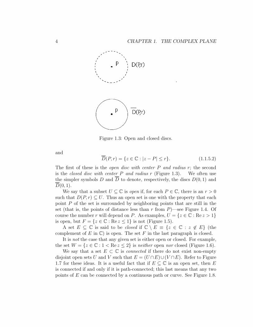
Figure 1.3: Open and closed discs.
andD(P, r) = {z ∈ C : |z − P | ≤ r}. (1.1.5.2)
The first of these is the open disc with center P and radius r; the secondis the closed disc with center P and radius r (Figure 1.3). We often usethe simpler symbols D and D to denote, respectively, the discs D(0, 1) andD(0, 1).
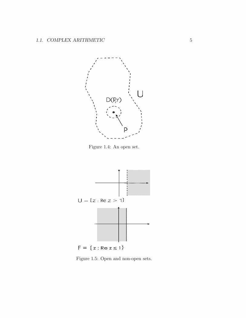
We say that a subset U ⊆ C is open if, for each P ∈ C, there is an r > 0such that D(P, r) ⊆ U . Thus an open set is one with the property that eachpoint P of the set is surrounded by neighboring points that are still in theset (that is, the points of distance less than r from P )—see Figure 1.4. Ofcourse the number r will depend on P . As examples, U = {z ∈ C : Re z > 1}is open, but F = {z ∈ C : Re z ≤ 1} is not (Figure 1.5).
A set E ⊆ C is said to be closed if C \ E ≡ {z ∈ C : z 6∈ E} (thecomplement of E in C) is open. The set F in the last paragraph is closed.
It is not the case that any given set is either open or closed. For example,the set W = {z ∈ C : 1 < Re z ≤ 2} is neither open nor closed (Figure 1.6).
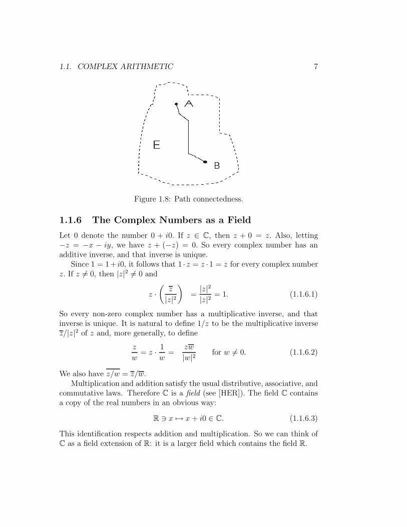
We say that a set E ⊂ C is connected if there do not exist non-emptydisjoint open sets U and V such that E = (U ∩E)∪ (V ∩E). Refer to Figure1.7 for these ideas. It is a useful fact that if E ⊆ C is an open set, then Eis connected if and only if it is path-connected; this last means that any twopoints of E can be connected by a continuous path or curve. See Figure 1.8.
1.1. COMPLEX ARITHMETIC 5
Figure 1.4: An open set.
Figure 1.5: Open and non-open sets.

6 CHAPTER 1. THE COMPLEX PLANE
Figure 1.6: A set that is neither open nor closed.
Figure 1.7: The concept of connectivity.
1.1. COMPLEX ARITHMETIC 7
Figure 1.8: Path connectedness.
1.1.6 The Complex Numbers as a Field
Let 0 denote the number 0 + i0. If z ∈ C, then z + 0 = z. Also, letting−z = −x − iy, we have z + (−z) = 0. So every complex number has anadditive inverse, and that inverse is unique.
Since 1 = 1+ i0, it follows that 1 · z = z ·1 = z for every complex numberz. If z 6= 0, then |z|2 6= 0 and
z ·(
z
|z|2)
=|z|2|z|2 = 1. (1.1.6.1)
So every non-zero complex number has a multiplicative inverse, and thatinverse is unique. It is natural to define 1/z to be the multiplicative inversez/|z|2 of z and, more generally, to define
z
w= z · 1
w=
zw
|w|2 for w 6= 0. (1.1.6.2)
We also have z/w = z/w.Multiplication and addition satisfy the usual distributive, associative, and
commutative laws. Therefore C is a field (see [HER]). The field C containsa copy of the real numbers in an obvious way:
R 3 x 7→ x+ i0 ∈ C. (1.1.6.3)
This identification respects addition and multiplication. So we can think ofC as a field extension of R: it is a larger field which contains the field R.

8 CHAPTER 1. THE COMPLEX PLANE
1.1.7 The Fundamental Theorem of Algebra
It is not true that every non-constant polynomial with real coefficients has areal root. For instance, p(x) = x2 + 1 has no real roots. The FundamentalTheorem of Algebra states that every polynomial with complex coefficientshas a complex root (see the treatment in §§3.1.4 below). The complex fieldC is the smallest field that contains R and has this so-called algebraic clo-sure property. One of the first powerful and elegant applications of complexvariable theory is to provide a proof of the Fundamental Theorem of Algebra.
1.2 The Exponential and Applications
1.2.1 The Exponential Function
We define the complex exponential as follows:
(1.2.1.1) If z = x is real, then
ez = ex ≡∞∑
j=0
xj
j!
as in calculus. Here ! denotes “factorial”: j! = j·(j−1)·(j−2) · · · 3·2·1.
(1.2.1.2) If z = iy is pure imaginary, then
ez = eiy ≡ cos y + i sin y.
(1.2.1.3) If z = x+ iy, then
ez = ex+iy ≡ ex · eiy = ex · (cos y + i sin y).
Part and parcel of the last definition of the exponential is the followingcomplex-analytic definition of the sine and cosine functions:
cos z =eiz + e−iz
2, (1.2.1.4)
sin z =eiz − e−iz
2i. (1.2.1.5)

1.2. THE EXPONENTIAL AND APPLICATIONS 9
Note that when z = x + i0 is real this new definition coincides with thefamiliar Euler formula from calculus:
eit = cos t+ i sin t . (1.2.1.6)
1.2.2 The Exponential Using Power Series
It is also possible to define the exponential using power series:
ez =
∞∑
j=0
zj
j!. (1.2.2.1)
Either definition (that in §§1.2.1 or in §§1.2.2) is correct for any z, and theyare logically equivalent.
1.2.3 Laws of Exponentiation
The complex exponential satisfies familiar rules of exponentiation:
ez+w = ez · ew and (ez)w = ezw. (1.2.3.1)
Also (ez)n
= ez · · · ez︸ ︷︷ ︸n times
= enz. (1.2.3.2)
One may verify these properties directly from the power series definition, orelse use the more explicit definitions in (1.2.1.1)–(1.2.1.3).
1.2.4 Polar Form of a Complex Number
A consequence of our first definition of the complex exponential —see (1.2.1.2)—is that if ζ ∈ C, |ζ| = 1, then there is a unique number θ, 0 ≤ θ < 2π, suchthat ζ = eiθ (see Figure 1.9). Here θ is the (signed) angle between the positive
x axis and the ray−→0ζ.
Now, if z is any non-zero complex number, then
z = |z| ·(z
|z|
)≡ |z| · ζ , (1.2.4.1)

10 CHAPTER 1. THE COMPLEX PLANE
Figure 1.9: Polar representation of a complex number of modulus 1.
where ζ = z/|z| has modulus 1. Again letting θ be the angle between the
real axis and−→0ζ , we see that
z = |z| · ζ= |z|eiθ
= reiθ , (1.2.4.2)
where r = |z|. This form is called the polar representation for the complexnumber z. (Note that some classical books write the expression z = reiθ =r(cos θ + i sin θ) as z = rcis θ. The reader should be aware of this notation,though we shall not use it in this book.) Engineers like the cis notation.
EXAMPLE 1.2.4.1 Let z = 1 +√
3i. Then |z| =√
12 + (√
3)2 = 2.
Hence
z = 2 ·(
1
2+ i
√3
2
).
The unit-modulus number in parenthesis subtends an angle of π/3 with thepositive x-axis. Therefore
1 +√
3i = z = 2 · eiπ/3.

1.2. THE EXPONENTIAL AND APPLICATIONS 11
It is often convenient to allow angles that are greater than or equal to2π in the polar representation; when we do so, the polar representation is nolonger unique. For if k is an integer, then
eiθ = cos θ + i sin θ
= cos(θ + 2kπ) + i sin(θ + 2kπ)
= ei(θ+2kπ) . (1.2.4.3)
1.2.5 Roots of Complex Numbers
The properties of the exponential operation can be used to find the nth rootsof a complex number.
EXAMPLE 1.2.5.1 To find all sixth roots of 2, we let reiθ be an arbitrarysixth root of 2 and solve for r and θ. If
(reiθ)6
= 2 = 2 · ei0 (1.2.5.1.1)
orr6ei6θ = 2 · ei0 , (1.2.5.1.2)
then it follows that r = 21/6 ∈ R and θ = 0 solve this equation. So the realnumber 21/6 · ei0 = 21/6 is a sixth root of two. This is not terribly surprising,but we are not finished.
We may also solver6ei6θ = 2 = 2 · e2πi. (1.2.5.1.3)
Hencer = 21/6 , θ = 2π/6 = π/3. (1.2.5.1.4)
This gives us the number
21/6eiπ/3 = 21/6(cosπ/3 + i sinπ/3
)= 21/6
(1
2+ i
√3
2
)(1.2.5.1.5)
as a sixth root of two. Similarly, we can solve
r6ei6θ = 2 · e4πi
r6ei6θ = 2 · e6πi
r6ei6θ = 2 · e8πi
r6ei6θ = 2 · e10πi
12 CHAPTER 1. THE COMPLEX PLANE
to obtain the other four sixth roots of 2:
21/6
(−1
2+ i
√3
2
)(1.2.5.1.6)
−21/6 (1.2.5.1.7)
21/6
(−1
2− i
√3
2
)(1.2.5.1.8)
21/6
(1
2− i
√3
2
). (1.2.5.1.9)
These are in fact all the sixth roots of 2.
Remark: One could of course continue the procedure in the last example,solving r6ei6θ = 2 · e12πi, etc.. But this would simply result in repetition ofthe roots we have already found.
EXAMPLE 1.2.5.2 Let us find all third roots of i. We begin by writingi as
i = eiπ/2. (1.2.5.2.1)
Solving the equation
(reiθ)3 = i = eiπ/2 (1.2.5.2.2)
then yields r = 1 and θ = π/6.
Next, we write i = ei5π/2 and solve
(reiθ)3 = ei5π/2 (1.2.5.2.3)
to obtain that r = 1 and θ = 5π/6.
Lastly, we write i = ei9π/2 and solve
(reiθ)3 = ei9π/2 (1.2.5.2.4)
to obtain that r = 1 and θ = 9π/6 = 3π/2.

1.2. THE EXPONENTIAL AND APPLICATIONS 13
6
2
Figure 1.10: The sixth roots of 2.
In summary, the three cube roots of i are
eiπ/6 =
√3
2+ i
1
2, (1.2.5.2.5)
ei5π/6 = −√
3
2+ i
1
2, (1.2.5.2.6)
ei3π/2 = −i . (1.2.5.2.7)
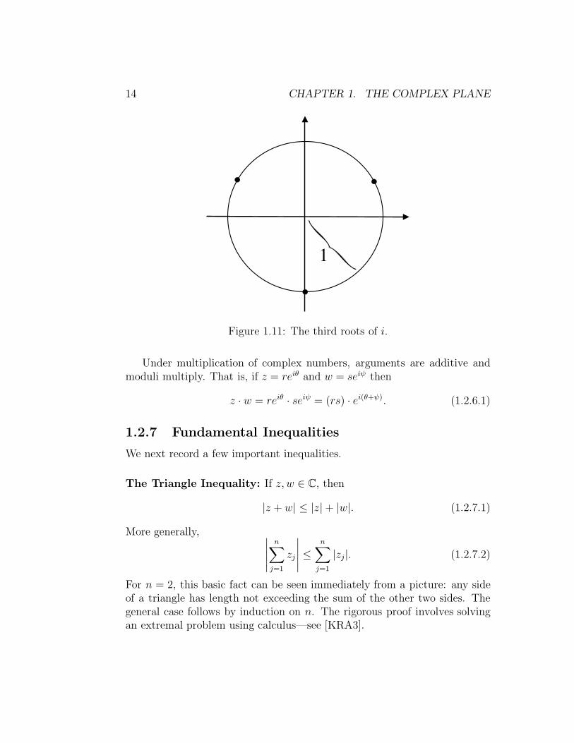
It is worth noting that, in both Examples 1.2.5.1 and 1.2.5.2, the roots ofthe given complex number are equally spaced about a circle centered at theorigin. See Figures 1.10 and 1.11.
1.2.6 The Argument of a Complex Number
The (non-unique) angle θ associated to a complex number z 6= 0 is called itsargument, and is written arg z. For instance, arg(1 + i) = π/4. But it is alsocorrect to write arg(1 + i) = 9π/4, 17π/4,−7π/4, etc. We generally choosethe argument θ to satisfy 0 ≤ θ < 2π. This is the principal branch of theargument—see §§9.1.2, §§9.4.2.
14 CHAPTER 1. THE COMPLEX PLANE
1
Figure 1.11: The third roots of i.
Under multiplication of complex numbers, arguments are additive andmoduli multiply. That is, if z = reiθ and w = seiψ then
z · w = reiθ · seiψ = (rs) · ei(θ+ψ). (1.2.6.1)
1.2.7 Fundamental Inequalities
We next record a few important inequalities.
The Triangle Inequality: If z, w ∈ C, then
|z + w| ≤ |z| + |w|. (1.2.7.1)
More generally, ∣∣∣∣∣
n∑
j=1
zj
∣∣∣∣∣ ≤n∑
j=1
|zj|. (1.2.7.2)
For n = 2, this basic fact can be seen immediately from a picture: any sideof a triangle has length not exceeding the sum of the other two sides. Thegeneral case follows by induction on n. The rigorous proof involves solvingan extremal problem using calculus—see [KRA3].

1.3. HOLOMORPHIC FUNCTIONS 15
The Cauchy-Schwarz Inequality: If z1, . . . , zn and w1, . . . , wn are com-plex numbers, then
∣∣∣∣∣
n∑
j=1
zjwj
∣∣∣∣∣
2
≤[
n∑
j=1
|zj|2]·[
n∑
j=1
|wj|2]. (1.2.7.3)
This result is immediate from the Triangle Inequality: Just square both sidesand multiply everything out.
1.3 Holomorphic Functions
1.3.1 Continuously Differentiable and Ck Functions
In this book we will frequently refer to a domain or a region U ⊆ C. Usuallythis will mean that U is an open set and that U is connected (see §1.1.5).
Holomorphic functions are a generalization of complex polynomials. Butthey are more flexible objects than polynomials. The collection of all poly-nomials is closed under addition and multiplication. However, the collectionof all holomorphic functions is closed under reciprocals, inverses, exponenti-ation, logarithms, square roots, and many other operations as well.
There are several different ways to introduce the concept of holomorphicfunction. It can be defined by way of power series, or using the complexderivative, or using partial differential equations. We shall touch on all theseapproaches; but our initial definition will be by way of partial differentialequations. First ewe need some preliminary concepts from real analysis.
If U ⊆ R2 is open and f : U → R is a continuous function, then f iscalled C1 (or continuously differentiable) on U if ∂f/∂x and ∂f/∂y exist andare continuous on U. We write f ∈ C1(U) for short.
More generally, if k ∈ {0, 1, 2, ...}, then a real-valued function f on U iscalled Ck (k times continuously differentiable) if all partial derivatives of fup to and including order k exist and are continuous on U. We write in thiscase f ∈ Ck(U). In particular, a C0 function is just a continuous function.
A function f = u+ iv : U → C is called Ck if both u and v are Ck.
1.3.2 The Cauchy-Riemann Equations
If f is any complex-valued function, then we may write f = u+ iv, where uand v are real-valued functions.
16 CHAPTER 1. THE COMPLEX PLANE
EXAMPLE 1.3.2.1 Consider
f(z) = z2 = (x2 − y2) + i(2xy);
in this example u = x2 − y2 and v = 2xy. We refer to u as the real part of fand denote it by Re f ; we refer to v as the imaginary part of f and denote itby Im f .
Now we formulate the notion of “holomorphic function” in terms of thereal and imaginary parts of f :
Let U ⊆ C be an open set and f : U → C a C1 function. Write
f(z) = f(x+ iy) ≡ f(x, y) = u(x, y) + iv(x, y),
with z = x + iy and u and v real-valued functions. If u and v satisfy theequations
∂u
∂x=∂v
∂y
∂u
∂y= −∂v
∂x(1.3.2.2)
at every point of U , then the function f is said to be holomorphic (see §§1.3.4,where a formal definition of “holomorphic” is provided). The first order, lin-ear partial differential equations in (1.3.2.2) are called the Cauchy-Riemannequations. A practical method for checking whether a given function is holo-morphic is to check whether it satisfies the Cauchy-Riemann equations. An-other intuitively appealing method, which we develop in the next subsection,is to verify that the function in question depends on z only and not on z.
1.3.3 Derivatives
We define, for f = u+ iv : U → C a C1 function,
∂
∂zf ≡ 1
2
(∂
∂x− i
∂
∂y
)f =
1
2
(∂u
∂x+∂v
∂y
)+i
2
(∂v
∂x− ∂u
∂y
)(1.3.3.1)
and
∂
∂zf ≡ 1
2
(∂
∂x+ i
∂
∂y
)f =
1
2
(∂u
∂x− ∂v
∂y
)+i
2
(∂v
∂x+∂u
∂y
). (1.3.3.2)
If z = x+ iy, z = x− iy, then one can check directly that

1.3. HOLOMORPHIC FUNCTIONS 17
∂
∂zz = 1 ,
∂
∂zz = 0 ,
(1.3.3.3)
∂
∂zz = 0 ,
∂
∂zz = 1 .
If a C1 function f satisfies ∂f/∂z ≡ 0 on an open set U , then f doesnot depend on z (but it does depend on z). If instead f satisfies ∂f/∂z ≡ 0on an open set U , then f does not depend on z (but it does depend onz). The condition ∂f/∂z = 0 is a reformulation of the Cauchy-Riemannequations—see §§1.3.4.
1.3.4 Definition of Holomorphic Function
Functions f that satisfy (∂/∂z)f ≡ 0 are the main concern of complex anal-ysis. A continuously differentiable (C1) function f : U → C defined on anopen subset U of C is said to be holomorphic if
∂f
∂z= 0 (1.3.4.1)
at every point of U. Note that this last equation is just a reformulation ofthe Cauchy-Riemann equations (§§1.3.2). To see this, we calculate:
0 =∂
∂zf(z)
=1
2
(∂
∂x+ i
∂
∂y
)[u(z) + iv(z)]
=
[∂u
∂x− ∂v
∂y
]+ i
[∂u
∂y+∂v
∂x
]. (1.3.4.2)
Of course the far right-hand side cannot be identically zero unless each of itsreal and imaginary parts is identically zero. It follows that
∂u
∂x− ∂v
∂y= 0
18 CHAPTER 1. THE COMPLEX PLANE
and∂u
∂y+∂v
∂x= 0.
These are the Cauchy-Riemann equations (1.3.2.2).
1.3.5 The Complex Derivative
Let U ⊆ C be open, P ∈ U, and g : U \ {P} → C a function. We say that
limz→P
g(z) = ` , ` ∈ C , (1.3.5.1)
if for any ε > 0 there is a δ > 0 such that when z ∈ U and 0 < |z − P | < δthen |g(z) − `| < ε. This is similar to the calculus definition of limit, but itallows z to approach P from any direction.
We say that f possesses the complex derivative at P if
limz→P
f(z) − f(P )
z − P(1.3.5.2)
exists. In that case we denote the limit by f ′(P ) or sometimes by
df
dz(P ) or
∂f
∂z(P ). (1.3.5.3)
This notation is consistent with that introduced in §§1.3.3: for a holomorphicfunction, the complex derivative calculated according to formula (1.3.5.2) oraccording to formula (1.3.3.1) is just the same (use the Cauchy-Riemannequations). We shall say more about the complex derivative in §2.2.3 and§2.2.4.
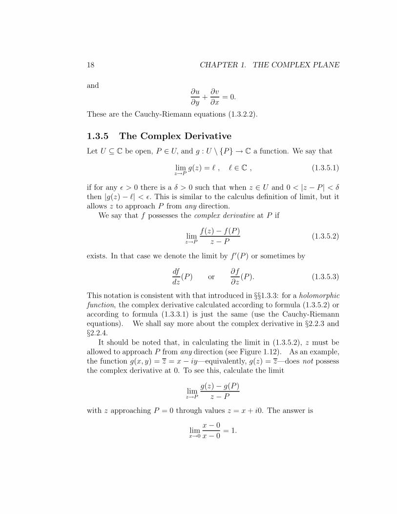
It should be noted that, in calculating the limit in (1.3.5.2), z must beallowed to approach P from any direction (see Figure 1.12). As an example,the function g(x, y) = z = x − iy—equivalently, g(z) = z—does not possessthe complex derivative at 0. To see this, calculate the limit
limz→P
g(z) − g(P )
z − P
with z approaching P = 0 through values z = x+ i0. The answer is
limx→0
x− 0
x− 0= 1.

1.3. HOLOMORPHIC FUNCTIONS 19
P
zz
Figure 1.12: The limit from any direction.
If instead z is allowed to approach P = 0 through values z = iy, then thevalue is
limy→0
−iy − 0
iy − 0= −1.
Observe that the two answers do not agree. In order for the complex deriva-tive to exist, the limit must exist and assume only one value no matter howz approaches P . Therefore this example g does not possess the complexderivative at P = 0. In fact a similar calculation shows that this function gdoes not possess the complex derivative at any point.
If a function f possesses the complex derivative at every point of its opendomain U , then f is holomorphic. This definition is equivalent to definitionsgiven in §§1.3.2, §§1.3.4. We repeat some of these ideas in §2.2.
1.3.6 Alternative Terminology for Holomorphic Func-
tions
Some books use the word “analytic” instead of “holomorphic.” Still otherssay “differentiable” or “complex differentiable” instead of “holomorphic.”The use of the term “analytic” derives from the fact that a holomorphicfunction has a local power series expansion about each point of its domain(see §§3.1.6). In fact this power series property is a complete characterizationof holomorphic functions; we shall discuss it in detail below. The use of“differentiable” derives from properties related to the complex derivative.These pieces of terminology and their significance will all be sorted out asthe book develops. Somewhat archaic terminology for holomorphic functions,which may be found in older texts, are “regular” and “monogenic.”
Another piece of terminology that is applied to holomorphic functions

20 CHAPTER 1. THE COMPLEX PLANE
is “conformal” or “conformal mapping.” “Conformality” is an importantgeometric property of holomorphic functions that make these functions usefulfor modeling incompressible fluid flow and other physical phenomena. Weshall discuss conformality in §§2.2.5. See also [KRA6].
1.4. HOLOMORPHIC AND HARMONIC FUNCTIONS 21
1.4 Holomorphic and Harmonic Functions
1.4.1 Harmonic Functions
A C2 function u is said to be harmonic if it satisfies the equation
(∂2
∂x2+
∂2
∂y2
)u = 0. (1.4.1.1)
This equation is called Laplace’s equation, and is frequently abbreviated as
4u = 0. (1.4.1.2)
1.4.2 How They are Related
If f is a holomorphic function and f = u+ iv is the expression of f in termsof its real and imaginary parts, then both u and v are harmonic. An elegantway to see this is to observe that
∂
∂zf = 0
hence∂
∂z
∂
∂zf = 0 .
But we may write out the lefthand side of the last equation to find that
1
44 f = 0
or
(4u) + i(4v) = 0 .
It is important to note here that the Laplacian 4 is a real operator. Thusthe only way that the last identity can be true is if
4u = 0 and 4 v = 0 .
This is what we have asserted.A converse is true provided the functions involved are defined on a domain
with no holes:

22 CHAPTER 1. THE COMPLEX PLANE
Theorem: If R is an open rectangle (or open disc) and if u isa real-valued harmonic function on R, then there is a holomorphicfunction F on R such that ReF = u. In other words, for such afunction u there exists a harmonic function v defined on R suchthat f ≡ u+ iv is holomorphic on R. Any two such functions vmust differ by a real constant.
More generally, if U is a region with no holes (a simply con-nected region—see §§2.3.3), and if u is harmonic on U , then thereis a holomorphic function F on U with ReF = u. In other words,for such a function u there exists a harmonic function v definedon U such that f ≡ u + iv is holomorphic on U . Any two suchfunctions v must differ by a constant. We call the function v aharmonic conjugate for u.
To give an indication of why these statements are true we note that, givenu harmonic, we seek v such that
∂v
∂x= −∂u
∂y≡ α(x, y)
and∂v
∂y=∂u
∂x≡ β(x, y)
(these are the Cauchy-Riemann equations). We know from calculus that apair of equations like this is solvable on a region with no holes precisely when
∂α
∂y=∂β
∂x.
But this last is just the condition that u be harmonic. This explains why v,and hence F = u+ iv, exists.
The displayed theorem is false on a domain with a hole, such as an annu-lus. For example, the harmonic function u = log(x2 + y2), defined on theannulus U = {z : 1 < |z| < 2}, has no harmonic conjugate on U . See also§§7.1.4.

Chapter 2
Complex Line Integrals
2.1 Real and Complex Line Integrals
In this section we shall recast the line integral from calculus in complexnotation. The result will be the complex line integral. The complex lineintegral is essential to the Cauchy theory, which we develop below, and thatin turn is key to the argument principle and many of the other central ideasof the subject.
2.1.1 Curves
It is convenient to think of a curve as a continuous function γ from a closedinterval [a, b] ⊆ R into R2 ≈ C. We sometimes let γ denote the image of themapping. Thus
γ = {γ(t) : t ∈ [a, b]} .Often we follow the custom of referring to either the function or the imagewith the single symbol γ. It will be clear from context what is meant. Referto Figure 2.1.
It is often convenient to write
γ(t) = (γ1(t), γ2(t)) or γ(t) = γ1(t) + iγ2(t). (2.1.1.1)
For example, γ(t) = (cos t, sin t) = cos t + i sin t, t ∈ [0, 2π], describes theunit circle in the plane. The circle is traversed in a counterclockwise manneras t increases from 0 to 2π. Again see Figure 2.1.
23

24 CHAPTER 2. COMPLEX LINE INTEGRALS
Figure 2.1: Curves in the plane.
2.1.2 Closed Curves
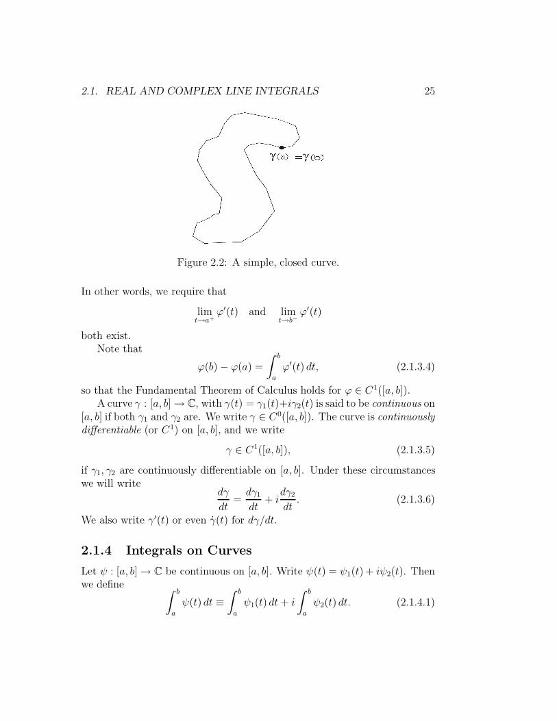
The curve γ : [a, b] → C is called closed if γ(a) = γ(b). It is called simple,closed (or Jordan) if the restriction of γ to the interval [a, b) (which is com-monly written γ
∣∣[a,b)
) is one-to-one and γ(a) = γ(b) (Figure 2.2). Intuitively,
a simple, closed curve is a curve with no self-intersections, except of coursefor the closing up at t = a, b.
In order to work effectively with γ we need to impose on it some differ-entiability properties.
2.1.3 Differentiable and Ck Curves
A function ϕ : [a, b] → R is called continuously differentiable (or C1), and wewrite ϕ ∈ C1([a, b]), if
(2.1.3.1) ϕ is continuous on [a, b];
(2.1.3.2) ϕ′ exists on (a, b);
(2.1.3.3) ϕ′ has a continuous extension to [a, b].
2.1. REAL AND COMPLEX LINE INTEGRALS 25
Figure 2.2: A simple, closed curve.
In other words, we require that
limt→a+
ϕ′(t) and limt→b−
ϕ′(t)
both exist.Note that
ϕ(b) − ϕ(a) =
∫ b
a
ϕ′(t) dt, (2.1.3.4)
so that the Fundamental Theorem of Calculus holds for ϕ ∈ C1([a, b]).A curve γ : [a, b] → C, with γ(t) = γ1(t)+iγ2(t) is said to be continuous on
[a, b] if both γ1 and γ2 are. We write γ ∈ C0([a, b]). The curve is continuouslydifferentiable (or C1) on [a, b], and we write
γ ∈ C1([a, b]), (2.1.3.5)
if γ1, γ2 are continuously differentiable on [a, b]. Under these circumstanceswe will write
dγ
dt=dγ1
dt+ i
dγ2
dt. (2.1.3.6)
We also write γ′(t) or even γ(t) for dγ/dt.
2.1.4 Integrals on Curves
Let ψ : [a, b] → C be continuous on [a, b]. Write ψ(t) = ψ1(t) + iψ2(t). Thenwe define ∫ b
a
ψ(t) dt ≡∫ b
a
ψ1(t) dt+ i
∫ b
a
ψ2(t) dt. (2.1.4.1)

26 CHAPTER 2. COMPLEX LINE INTEGRALS
We summarize the ideas presented thus far by noting that if γ ∈ C1([a, b])is complex-valued, then
γ(b) − γ(a) =
∫ b
a
γ′(t) dt. (2.1.4.2)
2.1.5 The Fundamental Theorem of Calculus along Curves
Now we state the Fundamental Theorem of Calculus (see [BKR]) adapted tocurves.
Let U ⊆ C be a domain and let γ : [a, b] → U be a C1 curve. If f ∈ C1(U),then
f(γ(b)) − f(γ(a)) =
∫ b
a
(∂f
∂x(γ(t)) · dγ1
dt+∂f
∂y(γ(t)) · dγ2
dt
)dt. (2.1.5.1)
For the proof, simply reduce the assertion (2.1.5.1) to the analogous classicalassertion from the calculus.
2.1.6 The Complex Line Integral
When f is holomorphic, then formula (2.1.5.1) may be rewritten (using theCauchy-Riemann equations) as
f(γ(b)) − f(γ(a)) =
∫ b
a
∂f
∂z(γ(t)) · dγ
dt(t) dt, (2.1.6.1)
where, as earlier, we have taken dγ/dt to be dγ1/dt+ idγ2/dt.This latter result plays much the same role for holomorphic functions as
does the Fundamental Theorem of Calculus for functions from R to R. Theexpression on the right of (2.1.6.1) is called the complex line integral and isdenoted ∮
γ
∂f
∂z(z) dz . (2.1.6.2)
More generally, if g is any continuous function whose domain contains thecurve γ, then the complex line integral of g along γ is defined to be
∮
γ
g(z) dz ≡∫ b
a
g(γ(t)) · dγdt
(t) dt. (2.1.6.3)
2.1. REAL AND COMPLEX LINE INTEGRALS 27
The main point here is that∮dz entails an expression of the form γ′(t) dt in
the integrand. Thus the trajectory and orientation of the curve will play adecisive role in the calculation, interpretation, and meaning of the complexline integral.
The whole concept of complex line integral is central to our further con-siderations in later sections. We shall use integrals like the one on the rightof (2.1.6.3) even when f is not holomorphic; but we can be sure that theequality (2.1.6.1) holds only when f is holomorphic.
Note that when γ(a) = γ(b) = A (and the domain U is simply connected)then the lefthand side of (2.1.6.1) is automatically equal to 0; and the right-hand side is simply the complex line integral of f around a closed curve.So we have a preview of the Cauchy integral theorem (see §§2.3.1) in thiscontext.
2.1.7 Properties of Integrals
We conclude this section with some easy but useful facts about integrals.
(2.1.7.1) If ϕ : [a, b] → C is continuous, then
∣∣∣∣∫ b
a
ϕ(t) dt
∣∣∣∣ ≤∫ b
a
|ϕ(t)| dt. (2.1.7.1.1)
(2.1.7.2) If γ : [a, b] → C is a C1 curve and ϕ is a continuous function onthe curve γ, then
∣∣∣∣∮
γ
ϕ(z) dz
∣∣∣∣ ≤[maxt∈[a,b]
|ϕ(t)|]· `(γ) , (2.1.7.2.1)
where
`(γ) ≡∫ b
a
|ϕ′(t)| dt
is the length of γ. Note that (2.1.7.2.1) follows from (2.1.7.1.1), and (2.1.7.1.1)is just calculus.
(2.1.7.3) The calculation of a complex line integral is independent of theway in which we parametrize the path:
28 Chapter 2. Complex Line Integrals
Let U ⊆ C be an open set and f : U → C a continuousfunction. Let γ : [a, b] → U be a C1 curve. Suppose that ϕ :[c, d] → [a, b] is a one-to-one, onto, increasing C1 function with aC1 inverse. Let γ = γ ◦ ϕ. Then
∮
eγ
f dz =
∮
γ
f dz. (2.1.7.3.1)
The result follows from the change of variables formula in calculus.
This last statement implies that one can use the idea of the integral of afunction f along a curve γ when the curve γ is described geometrically butwithout reference to a specific parametrization. For instance, “the integral ofz counterclockwise around the unit circle {z ∈ C : |z| = 1}” is now a phrasethat makes sense, even though we have not indicated a specific parametriza-tion of the unit circle. Note, however, that the direction counts: The integralof z counterclockwise around the unit circle is 2πi. If the direction is reversed,then the integral changes sign: The integral of z clockwise around the unitcircle is −2πi.
2.2 Complex Differentiability and Conformal-
ity
2.2.1 Limits
Until now we have developed a complex differential and integral calculus.We now unify the notions of partial derivative and total derivative in thecomplex context. For convenience, we shall repeat some ideas from §1.3.
2.2.2 Holomorphicity and the Complex Derivative
Let U ⊆ C be an open set and let f be holomorphic on U . Then f ′ exists ateach point of U and
f ′(z) =∂f
∂z(2.2.4.1)
for all z ∈ U (where ∂f/∂z is defined as in §§1.3.3). This is because wesee that ∂f/∂x (according to the definition) coincides with df/dz and ∂f/∂y

2.2. Complex Differentiability 29
coincides with idf/dz. Hence
∂f
∂z=
1
2
(∂f
∂x− i
∂f
∂y
)=df
dz.
Note that, as a consequence, we can (and often will) write f ′ for ∂f/∂zwhen f is holomorphic. The following result is a converse:
If f ∈ C1(U) and f has a complex derivative f ′ at each point of U , then fis holomorphic on U . In particular, if a continuous, complex-valued functionf on U has a complex derivative at each point and, if f ′ is continuous on U ,then f is holomorphic on U . Such a function satisfies the Cauchy-Riemannequations (1.3.2.2).
It is perfectly logical to consider an f that possesses a complex derivativeat each point of U without the additional assumption that f ∈ C1(U). Itturns out that, under these circumstances, u and v still satisfy the Cauchy-Riemann equations. It is a deeper result, due to Goursat, that if f hasa complex derivative at each point of U , then f ∈ C1(U) and hence f isholomorphic. See [GRK], especially the Appendix on Goursat’s theorem, fordetails.
2.2.3 Conformality
Now we make some remarks about “conformality.” Stated loosely, a functionis conformal at a point P ∈ C if the function “preserves angles” at P and“stretches equally in all directions” at P . Holomorphic functions enjoy bothproperties. Now we shall discuss them in detail.
Let f be holomorphic in a neighborhood of P ∈ C. Let w1, w2 be complexnumbers of unit modulus. Consider the directional derivatives
Dw1f(P ) ≡ lim
t→0
f(P + tw1) − f(P )
t(2.2.5.1)
and
Dw2f(P ) ≡ lim
t→0
f(P + tw2) − f(P )
t. (2.2.5.2)
Then
(2.2.5.3) |Dw1f(P )| = |Dw2
f(P )| .

30 Chapter 2. Complex Line Integrals
(2.2.5.4) If |f ′(P )| 6= 0, then the directed angle from w1 to w2 equalsthe directed angle from Dw1
f(P ) to Dw2f(P ).
In fact the last statement has an important converse: If (2.2.5.4) holdsat P , then f has a complex derivative at P . If (2.2.5.3) holds at P , theneither f or f has a complex derivative at P . Thus a function that is confor-mal (in either sense) at all points of an open set U must possess the complexderivative at each point of U . By the discussion in §§2.2.4, f is thereforeholomorphic if it is C1. Or, by Goursat’s theorem, it would then follow thatthe function is holomorphic on U , with the C1 condition being automatic.
Proof of Conformality: Notice that
Dwjf(P ) = lim
t→0
f(P + twj) − f(P )
twj· twjt
= f ′(P ) · wj , j = 1, 2.
The first assertion is now immediate and the second follows from the usualgeometric interpretation of multiplication by a nonzero complex number,namely, that multiplication by reiθ, r 6= 0, multiplies lengths by r and ro-tates (around the origin) by the angle θ.
The converse to this theorem asserts in effect that if either of statements(2.2.4.2) or (2.2.4.3) holds at P , then f has a complex derivative at P . Thusa C1 function that is conformal (in either sense) at all points of an open setU must possess the complex derivative at each point of U . Of course then fis holomorphic if it is C1. We leave these assertions to the reader.
It is worthwhile to consider the theorem expressed in terms of real func-tions. That is, we write f = u+ iv, where u, v are real-valued functions. Alsowe consider f(x + iy), and hence u and v, as functions of the real variablesx and y. Thus f , as a function from an open subset of C into C, can beregarded as a function from an open subset of R2 into R2. With f viewedin these real-variable terms, the first derivative behavior of f is described byits Jacobian matrix:
∂u
∂x
∂u
∂y∂v
∂x
∂v
∂y
.

2.2. Complex Differentiability 31
Recall that this matrix, evaluated at a point (x0, y0), is the matrix of thelinear transformation that best approximates f(x, y) − f(x0, y0) at (x0, y0).Now the Cauchy-Riemann equations for f mean exactly that this matrix hasthe form (
a −bb a
).
Such a matrix is either the zero matrix or it can be written as the productof two matrices:
( √a2 + b2 0
0√a2 + b2
)·(
cos θ − sin θsin θ cos θ
)
for some choice of θ ∈ R. One chooses θ so that
cos θ =a√
a2 + b2,
sin θ =b√
a2 + b2.
Such a choice of θ is possible because(
a√a2 + b2
)2
+
(b√
a2 + b2
)2
= 1.
Thus the Cauchy-Riemann equations imply that the (real) Jacobian of f hasthe form (
λ 00 λ
)·(
cos θ − sin θsin θ cos θ
)
for some λ ∈ R, λ > 0, and some θ ∈ R.Geometrically, these two matrices have simple meanings. The matrix
(cos θ − sin θsin θ cos θ
)
is the representation of a rotation around the origin by the angle θ. Thematrix (
λ 00 λ
)
is multiplication of all vectors in R2 by λ. Therefore the product(λ 00 λ
)·(
cos θ − sin θsin θ cos θ
)

32 Chapter 2. Complex Line Integrals
represents the same operation on R2 as does multiplication on C by thecomplex number λeiθ.
Notice that, for our particular (Jacobian) matrix
∂u
∂x
∂u
∂y∂v
∂x
∂v
∂y
,
we have
λ =
√(∂u
∂x
)2
+
(∂v
∂x
)2
= |f ′(z)|,
in agreement with the theorem.
2.3 The Cauchy Integral Formula and Theo-
rem
2.3.1 The Cauchy Integral Theorem, Basic Form
If f is a holomorphic function on an open disc U in the complex plane, andif γ : [a, b] → U is a C1 curve in U with γ(a) = γ(b), then
∮
γ
f(z) dz = 0. (2.3.1.1)
There are a number of different ways to prove the Cauchy integral theo-rem. One of the most natural is by way of a complex-analytic form of Stokes’stheorem: If γ is a simple, closed curve surrounding a region U in the planethen ∮
γ
f(z) dz =
∫ ∫
U
∂f
∂zdz ∧ dz =
∫ ∫
U
0dz ∧ dz = 0 .
An important converse of Cauchy’s theorem is called Morera’s theorem:
Let f be a continuous function on a connected open set U ⊆ C.If
∮
γ
f(z) dz = 0 (2.3.1.2)

2.3. The Cauchy Integral Theorem 33
for every simple, closed curve γ in U , then f is holomorphic onU .
In the statement of Morera’s theorem, the phrase “every simple, closed curve”may be replaced by “every triangle” or “every square” or “every circle.”Morera’s theorem may also be proved using Stokes’s theorem (as above). Weleave the details to the reader, or see [GRK].
2.3.2 The Cauchy Integral Formula
Suppose that U is an open set in C and that f is a holomorphic function onU . Let z0 ∈ U and let r > 0 be such that D(P, r) ⊆ U . Let γ : [0, 1] → C bethe C1 curve γ(t) = P + r cos(2πt)+ ir sin(2πt). Then, for each z ∈ D(P, r),
f(z) =1
2πi
∮
γ
f(ζ)
ζ − zdζ. (2.3.2.1)
One may derive this result directly from Stokes’s theorem (see [KRA5] andalso our Subsection 2.3.1).
2.3.3 More General Forms of the Cauchy Theorems
Now we present the very useful general statements of the Cauchy integraltheorem and formula. First we need a piece of terminology. A curve γ :[a, b] → C is said to be piecewise Ck if
[a, b] = [a0, a1] ∪ [a1, a2] ∪ · · · ∪ [am−1, am] (2.3.3.1)
with a = a0 < a1 < · · · am = b and γ∣∣[aj−1,aj]
is Ck for 1 ≤ j ≤ m. In other
words, γ is piecewise Ck if it consists of finitely many Ck curves chained endto end.
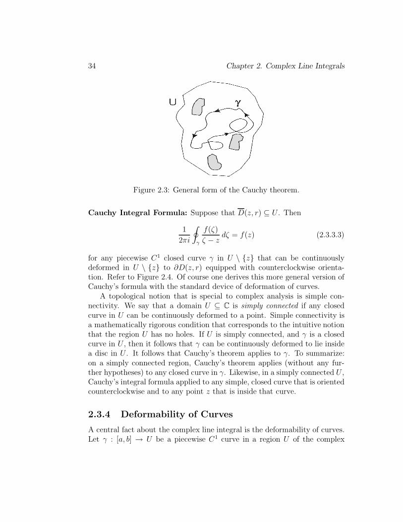
Cauchy Integral Theorem: Let f : U → C be holomorphic with U ⊆ C
an open set. Then ∮
γ
f(z) dz = 0 (2.3.3.2)
for each piecewise C1 closed curve γ in U that can be deformed in U throughclosed curves to a point in U—see Figure 2.3.
34 Chapter 2. Complex Line Integrals
Figure 2.3: General form of the Cauchy theorem.
Cauchy Integral Formula: Suppose that D(z, r) ⊆ U . Then
1
2πi
∮
γ
f(ζ)
ζ − zdζ = f(z) (2.3.3.3)
for any piecewise C1 closed curve γ in U \ {z} that can be continuouslydeformed in U \ {z} to ∂D(z, r) equipped with counterclockwise orienta-tion. Refer to Figure 2.4. Of course one derives this more general version ofCauchy’s formula with the standard device of deformation of curves.
A topological notion that is special to complex analysis is simple con-nectivity. We say that a domain U ⊆ C is simply connected if any closedcurve in U can be continuously deformed to a point. Simple connectivity isa mathematically rigorous condition that corresponds to the intuitive notionthat the region U has no holes. If U is simply connected, and γ is a closedcurve in U , then it follows that γ can be continuously deformed to lie insidea disc in U . It follows that Cauchy’s theorem applies to γ. To summarize:on a simply connected region, Cauchy’s theorem applies (without any fur-ther hypotheses) to any closed curve in γ. Likewise, in a simply connected U ,Cauchy’s integral formula applied to any simple, closed curve that is orientedcounterclockwise and to any point z that is inside that curve.
2.3.4 Deformability of Curves
A central fact about the complex line integral is the deformability of curves.Let γ : [a, b] → U be a piecewise C1 curve in a region U of the complex
2.4. THE LIMITATIONS OF THE CAUCHY FORMULA 35
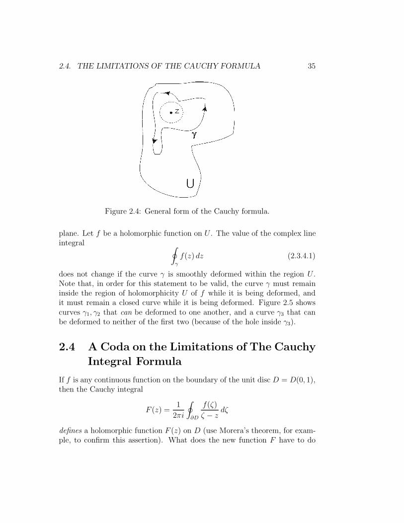
Figure 2.4: General form of the Cauchy formula.
plane. Let f be a holomorphic function on U . The value of the complex lineintegral ∮
γ
f(z) dz (2.3.4.1)
does not change if the curve γ is smoothly deformed within the region U .Note that, in order for this statement to be valid, the curve γ must remaininside the region of holomorphicity U of f while it is being deformed, andit must remain a closed curve while it is being deformed. Figure 2.5 showscurves γ1, γ2 that can be deformed to one another, and a curve γ3 that canbe deformed to neither of the first two (because of the hole inside γ3).
2.4 A Coda on the Limitations of The Cauchy
Integral Formula
If f is any continuous function on the boundary of the unit disc D = D(0, 1),then the Cauchy integral
F (z) =1
2πi
∮
∂D
f(ζ)
ζ − zdζ
defines a holomorphic function F (z) on D (use Morera’s theorem, for exam-ple, to confirm this assertion). What does the new function F have to do

36 Chapter 2. Complex Line Integrals
Figure 2.5: Deformation of curves.
with the original function f? In general, not much.For example, if f(ζ) = ζ, then F (z) ≡ 0 (exercise). In no sense is
the original function f any kind of “boundary limit” of the new functionF . The question of which functions f are “natural boundary functions” forholomorphic functions F (in the sense that F is a continuous extension of Fto the closed disc) is rather subtle. Its answer is well understood, but is bestformulated in terms of Fourier series and the so-called Hilbert transform.The complete story is given in [KRA1]. See also [GAR] for a discussion ofthe F. and M. Riesz theorem.
Contrast this situation for holomorphic function with the much moresuccinct and clean situation for harmonic functions (§7.3).


38 Chapter 2. Complex Line Integrals

Chapter 3
Applications of the CauchyTheory
3.1 The Derivatives of a Holomorphic Func-
tion
3.1.1 A Formula for the Derivative
Let U ⊆ C be an open set and let f be holomorphic on U . Then f ∈ C∞(U).Moreover, if D(P, r) ⊆ U and z ∈ D(P, r), then
(∂
∂z
)kf(z) =
k!
2πi
∮
|ζ−P |=r
f(ζ)
(ζ − z)k+1dζ, k = 0, 1, 2, . . . . (3.1.1.1)
This formula is obtained simply by differentiating the standard Cauchy for-mula (2.3.2.1) under the integral sign.
3.1.2 The Cauchy Estimates
If f is a holomorphic on a region containing the closed disc D(P, r) and if|f | ≤ M on D(P, r), then
∣∣∣∣∂k
∂zkf(P )
∣∣∣∣ ≤M · k!rk
. (3.1.2.1)
This is proved by direct estimation of the Cauchy formula (3.1.1.1).
39
40 CHAPTER 3. APPLICATIONS OF THE CAUCHY THEORY
3.1.3 Entire Functions and Liouville’s Theorem
A function f is said to be entire if it is defined and holomorphic on all of C,i.e., f : C → C is holomorphic. For instance, any holomorphic polynomial isentire, ez is entire, and sin z, cos z are entire. The function f(z) = 1/z is notentire because it is undefined at z = 0. [In a sense that we shall make preciselater (§4.1, ff.), this last function has a “singularity” at 0.] The question wewish to consider is: “Which entire functions are bounded?” This questionhas a very elegant and complete answer as follows:
Liouville’s Theorem A bounded entire function is constant.
Proof: Let f be entire and assume that |f(z)| ≤ M for all z ∈ C. Fix aP ∈ C and let r > 0. We apply the Cauchy estimate (3.1.2.1) for k = 1 onD(P, r). So ∣∣∣∣
∂
∂zf(P )
∣∣∣∣ ≤M · 1!r
. (3.1.3.1)
Since this inequality is true for every r > 0, we conclude that
∂f
∂z(P ) = 0.
Since P was arbitrary, we conclude that
∂f
∂z≡ 0.
Therefore f is constant.
The end of the last proof bears some commentary. We prove that ∂f/∂z ≡0. But we know, since f is holomorphic, that ∂f/∂z ≡ 0. It follows fromlinear algebra that ∂f/∂x ≡ 0 and ∂f/∂y ≡ 0. Then calculus tells us that fis constant.
The reasoning that establishes Liouville’s theorem can also be used toprove this more general fact: If f : C → C is an entire function and if forsome real number C and some positive integer k, it holds that
|f(z)| ≤ C · (1 + |z|)k
for all z, then f is a polynomial in z of degree at most k.
3.1. The Derivatives of a Holomorphic Function 41
3.1.4 The Fundamental Theorem of Algebra
One of the most elegant applications of Liouville’s Theorem is a proof ofwhat is known as the Fundamental Theorem of Algebra (see also §§1.1.7):
The Fundamental Theorem of Algebra: Let p(z) be a non-constant (holomorphic) polynomial. Then p has a root. That is,there exists an α ∈ C such that p(α) = 0.
Proof: Suppose not. Then g(z) = 1/p(z) is entire. Also when |z| → ∞,then |p(z)| → +∞. Thus 1/|p(z)| → 0 as |z| → ∞; hence g is bounded.By Liouville’s Theorem, g is constant, hence p is constant. Contradiction.
The polynomial p has degree k ≥ 1, then let α1 denote the root providedby the Fundamental Theorem. By the Euclidean algorithm (see [HUN]), wemay divide z − α1 into p with no remainder to obtain
p(z) = (z − α1) · p1(z). (3.1.4.1)
Here p1 is a polynomial of degree k − 1 . If k − 1 ≥ 1, then, by the theorem,p1 has a root α2 . Thus p1 is divisible by (z − α2) and we have
p(z) = (z − α1) · (z − α2) · p2(z) (3.1.4.2)
for some polynomial p2(z) of degree k − 2. This process can be continueduntil we arrive at a polynomial pk of degree 0; that is, pk is constant. Wehave derived the following fact: If p(z) is a holomorphic polynomial of degreek, then there are k complex numbers α1, . . . αk (not necessarily distinct) anda non-zero constant C such that
p(z) = C · (z − α1) · · · (z − αk). (3.1.4.3)
If some of the roots of p coincide, then we say that p has multiple roots.To be specific, if m of the values αj1 , . . . , αjm are equal to some complexnumber α, then we say that p has a root of order m at α (or that p has aroot of multiplicity m at α). It is an easily verified fact that the polynomialp has a root of order m at α if p(α) = 0, p′(α) = 0, . . . p(m−1)(α) = 0 (wherethe parenthetical exponent denotes a derivative).

42 CHAPTER 3. APPLICATIONS OF THE CAUCHY THEORY
Figure 3.1: A compact set.
An example will make the idea clear: Let
p(z) = (z − 5)3 · (z + 2)8 · (z − 3i) · (z + 6).
Then we say that p has a root of order 3 at 5, a root of order 8 at −2, andit has roots of order 1 at 3i and at −6. We also say that p has simple rootsat 1 and −6.
3.1.5 Sequences of Holomorphic Functions and
their Derivatives
A sequence of functions gj defined on a common domain E is said to convergeuniformly to a limit function g if, for each ε > 0, there is a number N > 0such that for all j > N it holds that |gj(x)− g(x)| < ε for every x ∈ E. Thekey point is that the degree of closeness of gj(x) to g(x) is independent ofx ∈ E.
Let fj : U → C , j = 1, 2, 3 . . . , be a sequence of holomorphic functions onan open set U in C. Suppose that there is a function f : U → C such that, foreach compact subset E (a compact set is one that is closed and bounded—see Figure 3.1) of U , the restricted sequence fj|E converges uniformly to f |E .Then f is holomorphic on U . [In particular, f ∈ C∞(U).]
If fj, f, U are as in the preceding paragraph, then, for any k ∈ {0, 1, 2, . . . },we have (
∂
∂z
)kfj(z) →
(∂
∂z
)kf(z) (3.1.5.1)

3.1. The Derivatives of a Holomorphic Function 43
uniformly on compact sets.1 The proof is immediate from (3.1.1.1), which wederived from the Cauchy integral formula, for the derivative of a holomorphicfunction.
3.1.6 The Power Series Representation of a Holomor-phic Function
The ideas being considered in this section can be used to develop our under-standing of power series. A power series
∞∑
j=0
aj(z − P )j (3.1.6.1)
is defined to be the limit of its partial sums
SN (z) =N∑
j=0
aj(z − P )j. (3.1.6.2)
We say that the partial sums converge to the sum of the entire series.Any given power series has a disc of convergence. More precisely, let
r =1
lim supj→∞ |aj|1/j. (3.1.6.3)
The power series (3.1.6.2) will then certainly converge on the disc D(P, r);the convergence will be absolute and uniform on any disc D(P, r′) with r′ < r.
For clarity, we should point out that in many examples the sequence|aj|1/j actually converges as j → ∞. Then we may take r to be equal to1/ limj→∞ |aj|1/j. The reader should be aware, however, that in case thesequence {|aj|1/j} does not converge, then one must use the more formaldefinition (3.1.6.3) of r. See [KRA3], [RUD1].
Of course the partial sums, being polynomials, are holomorphic on anydisc D(P, r). If the disc of convergence of the power series is D(P, r), thenlet f denote the function to which the power series converges. Then for any0 < r′ < r we have that
SN (z) → f(z),
1It is also common to say that the functions converge normally.
44 CHAPTER 3. APPLICATIONS OF THE CAUCHY THEORY
uniformly on D(P, r′). We can conclude immediately that f(z) is holomor-phic on D(P, r). Moreover, we know that
(∂
∂z
)kSN (z) →
(∂
∂z
)kf(z). (3.1.6.4)
This shows that a differentiated power series has a disc of convergence atleast as large as the disc of convergence (with the same center) of the originalseries, and that the differentiated power series converges on that disc to thederivative of the sum of the original series.
The most important fact about power series for complex function theoryis this: If f is a holomorphic function on a domain U ⊆ C, if P ∈ U , and ifthe disc D(P, r) lies in U , then f may be represented as a convergent powerseries on D(P, r). Explicitly, we have
f(z) =∞∑
j=0
aj(z − P )j, (3.1.6.5)
where
aj =f (j)(P )
j!. (3.1.6.6)
[Here the exponent (j) on f denotes the jth derivative.] The provenance of thisformula will be explained below. Thus we have an explicit way of calculatingthe power series expansion of any holomorphic function f about a point Pof its domain, and we have an a priori knowledge of the disc on which thepower series representation will converge.
The matter bears further consideration. We know that every smoothfunction f(x) of a real variable has a Taylor series expansion about any pointp in the interior of its domain. But it is a fact that this Taylor expansiongenerically does not converge; even when it does converge, it genericallydoes not converge back to f . The situation for a holomorphic function of acomplex variable is markedly different: in that circumstance, the Taylor orpower series expansion always converges. The proof is simplicity itself. Takethe center of the disc in the Cauchy formula to be the origin 0. We write the

3.2. The Zeros of a Holomorphic Function 45
Cauchy formula as
f(z) =1
2πi
∮
∂D(0,r)
f(ζ)
ζ − zdζ
=
∮
∂D(0,r)
f(ζ) ·[1
ζ· 1
1 − z/ζ
]dζ
=
∮
∂D(0,r)
f(ζ) ·[
1
ζ·
∞∑
j=0
(z/ζ)j
]dζ
=
∮
∂D(0,r)
f(ζ) · 1
ζj+1dζ · zj
=∑
j
aj · zj .
We see explicitly that
aj =
∮
∂D(0,r)
f(ζ) · 1
ζj+1dζ ,
and this corresponds, by the Cauchy formula, to derivatives of f .
Of course the series converges absolutely and uniformly for |z| < r = |ζ|.The key point here is that holomorphic functions are analytic because theCauchy kernel is analytic. We know from our formula for the derivatives ofa holomorphic function that the jth coefficent of the power series in the lastexpansion is f (j)(0)/j!.
3.2 The Zeros of a Holomorphic Function
3.2.1 The Zero Set of a Holomorphic Function
Let f be a holomorphic function. If f is not identically zero, then it turnsout that f cannot vanish at too many points. This once again bears outthe dictum that holomorphic functions are a lot like polynomials. To givethis concept a precise formulation, we need to recall the topological notionof connectedness (§1.1.5).

46 CHAPTER 3. APPLICATIONS OF THE CAUCHY THEORY
3.2.2 Discreteness of the Zeros of a Holomorphic Func-
tion
Let U ⊆ C be a connected (§§1.1.5) open set and let f : U → C
be holomorphic. Let the zero set of f be Z = {z ∈ U : f(z) = 0}.If there are a z0 ∈ Z and {zj}∞j=1 ⊆ Z \ {z0} such that zj → z0,then f ≡ 0.
Let us formulate the result in topological terms. We recall that a pointz0 is said to be an accumulation point of a set Z if there is a sequence{zj} ⊆ Z \ {z0} with limj→∞ zj = z0. Then the theorem is equivalent to thestatement: If f : U → C is a holomorphic function on a connected (§§1.1.5)open set U and if Z = {z ∈ U : f(z) = 0} has an accumulation point in U ,then f ≡ 0.
For the proof, suppose that the point 0 is an interior accumulation pointof zeros {zj} of the holomorphic function f . Thus f(0) = 0. We may writef(z) = z · f∗(z). But f∗ vanishes at {zj} and 0 is still an accumulation pointof {zj}. It follows that f∗(0) = 0. Hence f itself has a zero of order 2 at 0.Continuing in this fashion, we see that f has a zero of infinite order at 0. Sothe power series expansion of f about 0 is identically 0. It then follows froman easy connectedness argument (more on this below) that f ≡ 0.
3.2.3 Discrete Sets and Zero Sets
There is still more terminology concerning the zero set of a holomorphicfunction in §§3.2.1. A set S is said to be discrete if for each s ∈ S there is anε > 0 such that D(s, ε)∩S = {s}. See Figure 3.2. People also say, in a slightabuse of language, that a discrete set has points that are “isolated” or that Scontains only “isolated points.” The result in §§3.2.2 thus asserts that if f isa non-constant holomorphic function on a connected open set, then its zeroset is discrete or, less formally, the zeros of f are isolated. It is important torealize that the result in §§3.2.2 does not rule out the possibility that the zeroset of f can have accumulation points in C \U ; in particular, a non-constantholomorphic function on an open set U can indeed have zeros accumulatingat a point of ∂U . Consider, for instance, the function f(z) = sin(1/[1−z]) onthe unit disc. The zeros of this f include {1− 1/[jπ]}, and these accumulateat the boundary point 1. See Figure 3.3.

3.2. The Zeros of a Holomorphic Function 47
Figure 3.2: A discrete set.
Figure 3.3: Zeros accumulating at a boundary point.

48 CHAPTER 3. APPLICATIONS OF THE CAUCHY THEORY
3.2.4 Uniqueness of Analytic Continuation
A consequence of the preceding basic fact (§§3.2.2) about the zeros of aholomorphic function is this: Let U ⊆ C be a connected open set andD(P, r) ⊆ U . If f is holomorphic on U and f
∣∣D(P,r)
≡ 0, then f ≡ 0 on
U . In fact if f ≡ 0 on a segment then it must follows that f ≡ 0.
Here are some further corollaries:
(3.2.4.1) Let U ⊆ C be a connected open set. Let f, g be holomorphic onU . If {z ∈ U : f(z) = g(z)} has an accumulation point in U , then f ≡ g.
(3.2.4.2) Let U ⊆ C be a connected open set and let f, g be holomorphic onU . If f · g ≡ 0 on U , then either f ≡ 0 on U or g ≡ 0 on U .
(3.2.4.3) Let U ⊆ C be connected and open and let f be holomorphic onU . If there is a P ∈ U such that
(∂
∂z
)jf(P ) = 0 (3.2.4.3.1)
for every j ∈ {0, 1, 2, . . . }, then f ≡ 0.
(3.2.4.4) If f and g are entire holomorphic functions and if f(x) = g(x) forall x ∈ R ⊆ C, then f ≡ g. It also holds that functional identities that aretrue for all real values of the variable are also true for complex values of thevariable (Figure 3.4). For instance,
sin2 z + cos2 z = 1 for all z ∈ C (3.2.4.4.1)
because the identity is true for all z = x ∈ R. This is an instance of the“principle of persistence of functional relations”—see [GRK].

3.2. The Zeros of a Holomorphic Function 49
Figure 3.4: Principle of persistence of functional relations.

50 CHAPTER 3. APPLICATIONS OF THE CAUCHY THEORY
Chapter 4
Isolated Singularities andLaurent Series
4.1 The Behavior of a Holomorphic Function
near an Isolated Singularity
4.1.1 Isolated Singularities
It is often important to consider a function that is holomorphic on a punc-tured open set U \ {P} ⊂ C. Refer to Figure 4.1.
In this chapter we shall obtain a new kind of infinite series expansionwhich generalizes the idea of the power series expansion of a holomorphicfunction about a (nonsingular) point—see §§3.1.6. We shall in the processcompletely classify the behavior of holomorphic functions near an isolatedsingular point (§§4.1.3).
4.1.2 A Holomorphic Function on a Punctured Do-
main
Let U ⊆ C be an open set and P ∈ U . We call the domain U \ {P} apunctured domain. Suppose that f : U \ {P} → C is holomorphic. In thissituation we say that f has an isolated singular point (or isolated singularity)at P . The implication of the phrase is usually just that f is defined andholomorphic on some such “deleted neighborhood” of P . The specificationof the set U is of secondary interest; we wish to consider the behavior of f
51
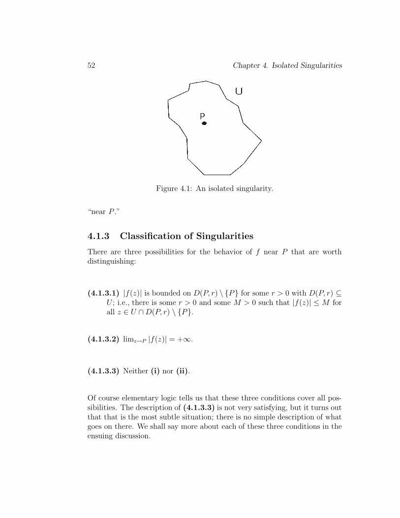
52 Chapter 4. Isolated Singularities
Figure 4.1: An isolated singularity.
“near P .”
4.1.3 Classification of Singularities
There are three possibilities for the behavior of f near P that are worthdistinguishing:
(4.1.3.1) |f(z)| is bounded on D(P, r) \ {P} for some r > 0 with D(P, r) ⊆U ; i.e., there is some r > 0 and some M > 0 such that |f(z)| ≤ M forall z ∈ U ∩D(P, r) \ {P}.
(4.1.3.2) limz→P |f(z)| = +∞.
(4.1.3.3) Neither (i) nor (ii).
Of course elementary logic tells us that these three conditions cover all pos-sibilities. The description of (4.1.3.3) is not very satisfying, but it turns outthat that is the most subtle situation; there is no simple description of whatgoes on there. We shall say more about each of these three conditions in theensuing discussion.

4.1. Behavior Near an Isolated Singularity 53
4.1.4 Removable Singularities, Poles, and Essential
Singularities
We shall see momentarily that, if case (4.1.3.1) holds, then f has a limit at Pthat extends f so that it is holomorphic on all of U (this is not at all obvious;it is a theorem of Riemann). It is commonly said in this circumstance that fhas a removable singularity at P . In case (4.1.3.2), we will say that f has apole at P. In case (4.1.3.3), f will be said to have an essential singularity atP. Our goal in this and the next two subsections is to understand (4.1.3.1)–(4.1.3.3) in some further detail.
4.1.5 The Riemann Removable Singularities Theorem
Let f : D(P, r) \ {P} → C be holomorphic and bounded. Then
(4.1.5.1) limz→P f(z) exists.
(4.1.5.2) The function f : D(P, r) → C defined by
f(z) =
{f(z) if z 6= P
limζ→P
f(ζ) if z = P
is holomorphic.
For the proof, take P = 0 and consider the function g(z) = z2 ·f(z). Onemay verify directly that g is C1 and satisfies the Cauchy-Riemann equationson all of D(P, r) (the boundedness hypothesis is used to check that both gand its first derivative have limits at 0). Thus g is holomorphic on the disc,and it vanishes to second order at 0. It follows then that f(z) = g(z)/z2 is abona fide holomorphic function on all of D(P, r).
4.1.6 The Casorati-Weierstrass Theorem
If f : D(P, r0) \ {P} → C is holomorphic and P is an essentialsingularity of f, then f(D(P, r) \ {P}) is dense in C for any0 < r < r0.
For the reason, suppose that the assertion is not true. So there is acomplex value µ and a positive number ε so that the image of D(P, r) \ {P}

54 Chapter 4. Isolated Singularities
under f does not contain the disc D(µ, ε). But then the function g(z) =1/[f(z) − µ] is bounded and non-vanishing near P , hence has a removablesingularity. We see then that f is bounded near P , and that contradicts thatP is an essential singularity.
Now we have seen that, at a removable singularity P , a holomorphicfunction f on D(P, r0) \ {P} can be continued to be holomorphic on all ofD(P, r0). And, near an essential singularity at P , a holomorphic function gon D(P, r0) \ {P} has image that is dense in C. The third possibility, that hhas a pole at P , has yet to be described. This case will be examined furtherin the coming sections.
We next develop a new type of doubly infinite series that will serve as atool for understanding isolated singularities—especially poles.
4.2 Expansion around Singular Points
4.2.1 Laurent Series
A Laurent series on D(P, r) is a (formal) expression of the form
+∞∑
j=−∞aj(z − P )j. (4.2.1.1)
Note that the individual terms are each defined for all z ∈ D(P, r) \ {P}.The series sums from j = −∞ to j = +∞.
4.2.2 Convergence of a Doubly Infinite Series
To discuss convergence of Laurent series, we must first make a general agree-ment as to the meaning of the convergence of a “doubly infinite” series∑+∞
j=−∞ αj. We say that such a series converges if∑+∞
j=0 αj and∑+∞
j=1 α−j =∑−1j=−∞ αj converge in the usual sense. In this case, we set
+∞∑
−∞αj =
(+∞∑
j=0
αj
)+
(+∞∑
j=1
α−j
). (4.2.2.1)
In other words, the question of convergence for a bi-infinite series devolvesto two separate questions about two sub-series.
We can now present the analogues for Laurent series of our basic resultsfor power series.

4.2. Expansion around Singular Points 55
4.2.3 Annulus of Convergence
The set of convergence of a Laurent series is either an open set of the form{z : 0 ≤ r1 < |z−P | < r2}, together with perhaps some or all of the boundarypoints of the set, or a set of the form {z : 0 ≤ r1 < |z−P | < +∞}, togetherwith perhaps some or all of the boundary points of the set. Such an open setis called an (generalized) annulus centered at P . We shall let
D(P,+∞) = {z : |z − P | < +∞} = C, (4.2.3.1)
D(P, 0) = {z : |z − P | < 0} = ∅, (4.2.3.2)
andD(P, 0) = {P}. (4.2.3.3)
As a result, using this extended notation, all (open) annuli (plural of “annu-lus”) can be written in the form
D(P, r2) \D(P, r1) , 0 ≤ r1 ≤ r2 ≤ +∞. (4.2.3.4)
In precise terms, the “domain of convergence” of a Laurent series is given asfollows:
Let+∞∑
j=−∞aj(z − P )j (4.2.3.5)
be a doubly infinite series. There are unique nonnegative extended realnumbers r1 and r2 (r1 or r2 may be 0 or +∞) such that the series con-verges absolutely for all z with r1 < |z − P | < r2 and diverges for z with|z − P | < r1 or |z − P | > r2 (see (4.2.3.4) ). Also, if r1 < s1 ≤ s2 < r2,then
∑+∞j=−∞ |aj(z−P )j| converges uniformly on {z : s1 ≤ |z−P | ≤ s2} and,
consequently,∑+∞
j=−∞ aj(z − P )j converges absolutely and uniformly there.The reason that the domain of convergence takes this form is that we
may rewrite the series (4.2.3.5) as
∞∑
j=0
aj(z − P )j +∞∑
j=1
a−j[(z − P )−1
]j.
From what we know about power series, the domain of convergence of thefirst of these two series will have the form |z − P | < r2 and the domainof convergence of the second series will have the form |(z − P )−1| < 1/r1.Putting these two conditions together gives r1 < |z − P | < r2.

56 Chapter 4. Isolated Singularities
4.2.4 Uniqueness of the Laurent Expansion
Let 0 ≤ r1 < r2 ≤ ∞. If the Laurent series∑+∞
j=−∞ aj(z − P )j converges on
D(P, r2) \D(P, r1) to a function f , then, for any r satisfying r1 < r < r2,and each j ∈ Z,
aj =1
2πi
∮
|ζ−P |=r
f(ζ)
(ζ − P )j+1dζ. (4.2.4.1)
This claim follows from integrating the series term-by-term (most of the termsintegrate to zero of course). In particular, the aj’s are uniquely determinedby f .
We turn now to establishing that convergent Laurent expansions of func-tions holomorphic on an annulus do in fact exist.
4.2.5 The Cauchy Integral Formula for an Annulus
Suppose that 0 ≤ r1 < r2 ≤ +∞ and that f : D(P, r2) \ D(P, r1) → C isholomorphic. Then, for each s1, s2 such that r1 < s1 < s2 < r2 and eachz ∈ D(P, s2) \D(P, s1), it holds that
f(z) =1
2πi
∮
|ζ−P |=s2
f(ζ)
ζ − zdζ − 1
2πi
∮
|ζ−P |=s1
f(ζ)
ζ − zdζ. (4.2.5.1)
Figure 4.2 shows why this is true. The integral along the two segments(which actually coincide, but with opposite orientations) vanishes. Whatis left is the integrals along the two circles—with opposite orientations, asindicated in (4.2.5.1).
4.2.6 Existence of Laurent Expansions
Now we may summarize with our main result:
Theorem: If 0 ≤ r1 < r2 ≤ ∞ and f : D(P, r2) \D(P, r1) → C
is holomorphic, then there exist complex numbers aj such that
+∞∑
j=−∞aj(z − P )j (4.2.6.1)
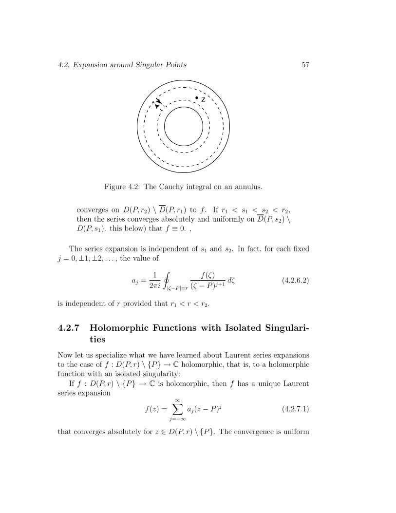
4.2. Expansion around Singular Points 57
z
Figure 4.2: The Cauchy integral on an annulus.
converges on D(P, r2) \ D(P, r1) to f . If r1 < s1 < s2 < r2,then the series converges absolutely and uniformly on D(P, s2) \D(P, s1). this below) that f ≡ 0. ,
The series expansion is independent of s1 and s2. In fact, for each fixedj = 0,±1,±2, . . . , the value of
aj =1
2πi
∮
|ζ−P |=r
f(ζ)
(ζ − P )j+1dζ (4.2.6.2)
is independent of r provided that r1 < r < r2.
4.2.7 Holomorphic Functions with Isolated Singulari-ties
Now let us specialize what we have learned about Laurent series expansionsto the case of f : D(P, r) \ {P} → C holomorphic, that is, to a holomorphicfunction with an isolated singularity:
If f : D(P, r) \ {P} → C is holomorphic, then f has a unique Laurentseries expansion
f(z) =∞∑
j=−∞aj(z − P )j (4.2.7.1)
that converges absolutely for z ∈ D(P, r) \ {P}. The convergence is uniform

58 Chapter 4. Isolated Singularities
on compact subsets of D(P, r) \ {P}. The coefficients are given by
aj =1
2πi
∮
∂D(P,s)
f(ζ)
(ζ − P )j+1dζ, any 0 < s < r. (4.2.7.2)
4.2.8 Classification of Singularities in Terms of Lau-
rent Series
There are three mutually exclusive possibilities for the Laurent series
∞∑
j=−∞aj(z − P )j
about an isolated singularity P :
(4.2.8.1) aj = 0 for all j < 0.
(4.2.8.2) For some k ≥ 1, aj = 0 for all −∞ < j < −k, but ak 6= 0.
(4.2.8.3) Neither (i) nor (ii) applies.
These three cases correspond exactly to the three types of isolated singu-larities that we discussed in §4.1.3: case (4.2.8.1) occurs if and only if P isa removable singularity; case (4.2.8.2) occurs if and only if P is a pole (oforder k, meaning that the term a−k in the Laurent expansion in nonzero—more on this below); and case (4.2.8.3) occurs if and only if P is an essentialsingularity.
To put this matter in other words: In case (4.2.8.1), we have a powerseries that converges, of course, to a holomorphic function. In case (4.2.8.2),our Laurent series has the form
∞∑
j=−kaj(z − P )j = (z − P )−k
∞∑
j=−kaj(z − P )j+k = (z − P )−k
∞∑
j=0
aj−k(z − P )j .
Since a−k 6= 0, we see that, for z near P , the function defined by the seriesbehaves like a−k · (z−P )−k near P . In short, the function (in absolute value)blows up like |z−P |−k as z → P . A graph in (|z|, |f(z)|)-space would exhibita “pole”-like singularity. This is the source of the terminology “pole.” SeeFigure 4.3. Case (4.2.8.3), corresponding to an essential singularity, is muchmore complicated; in this case there are infinitely many negative terms in

4.3. EXAMPLES OF LAURENT EXPANSIONS 59
Figure 4.3: A pole.
the Laurent expansion and, by Casorati-Weierstrass (§§4.1.6), they interactin a complicated fashion.
Picard’s Great Theorem (§§9.5.2) will tell us more about the behavior ofa holomorphic function near an essential singularity.
4.3 Examples of Laurent Expansions
4.3.1 Principal Part of a Function
When f has a pole or essential singularity at P, it is customary to call thenegative power part of the Laurent expansion of f around P the principalpart of f at P . (Occasionally we shall also use the terminology “Laurentpolynomial.”) That is, if
f(z) =
∞∑
j=−kaj(z − P )j (4.3.1.1)
for z near P , then the principal part of f at P is
−1∑
j=−kaj(z − P )j . (4.3.1.2)
As an example, the Laurent expansion about 0 of the function f(z) =

60 Chapter 4. Isolated Singularities
(z2 + 1)/ sin(z3) is
f(z) = (z2 + 1) · 1
sin(z3)
= (z2 + 1) · 1
z3· 1
1 − z6/3! + · · ·=
1
z3+
1
z+ (a holomorphic function).
The principal part of f is 1/z3 + 1/z.
For a second example, consider the function f(z) = (z2+2z+2) sin(1/(z+1)). Its Laurent expansion about the point −1 is
f(z) = ((z + 1)2 + 1) ·[
1
z + 1− 1
6(z + 1)3+
1
120(z + 1)5
− 1
5040(z + 1)7+ − · · ·
]
= (z + 1) +5
6
1
(z + 1)− 19
120
1
(z + 1)3+
41
5040
1
(z + 1)5− + · · · .
The principal part of f at the point −1 is
5
6
1
(z + 1)− 19
120
1
(z + 1)3+
41
5040
1
(z + 1)5− + · · · .
4.3.2 Algorithm for Calculating the Coefficients of the
Laurent Expansion
Let f be holomorphic on D(P, r) \ {P} and suppose that f has a pole oforder k at P . Then the Laurent series coefficients aj of f expanded aboutthe point P , for j = −k,−k + 1,−k + 2, . . . , are given by the formula
aj =1
(k + j)!
(∂
∂z
)k+j ((z − P )k · f
)∣∣∣∣z=P
. (4.3.2.1)
This formula is easily derived by considering the standard power seriescoefficients of (z − P )k · f(z).

4.4. THE CALCULUS OF RESIDUES 61
4.4 The Calculus of Residues
4.4.1 Functions with Multiple Singularities
It turns out to be useful, especially in evaluating various types of integrals,to consider functions that have more than one “singularity.” We want toconsider the following general question:
Suppose that f : U \ {P1, P2, . . . , Pn} → C is a holomorphicfunction on an open set U ⊆ C with finitely many distinct pointsP1, P2, . . . , Pn removed. Suppose further that
γ : [0, 1] → U \ {P1, P2, . . . , Pn} (4.4.1.1)
is a piecewiseC1 closed curve (§2.3.3) that (typically) “surrounds”some (but perhaps not all) of the points P1, . . . , Pn. Then how is∮γf related to the behavior of f near the points P1, P2, . . . , Pn?
The first step is to restrict our attention to open sets U for which∮γf is
necessarily 0 if P1, P2, . . . , Pn are removable singularities of f . See the nextsubsection.
4.4.2 The Residue Theorem
Suppose that U ⊆ C is a simply connected open set in C, and that P1, . . . , Pnare distinct points of U . Suppose that f : U \ {P1, . . . , Pn} → C is a holo-morphic function and γ is a piecewise C1 curve in U \ {P1, . . . , Pn}. Set
Rj = the coefficient of&(z − Pj)−1
in the Laurent expansion of f aboutPj . (4.4.2.1)
Then ∮
γ
f =n∑
j=1
Rj ·(∮
γ
1
ζ − Pjdζ
). (4.4.2.2)
To see this, first note that the integral over γ may be broken up intointegrals over “smaller curves,” each of which surrounds just one pole. SeeFigure 4.4. Then each such integral reduces, by deformation of curves, to anintegral around a circle. Thus the result is a straightforward calculation.

62 Chapter 4. Isolated Singularities
Figure 4.4: Reduction to simpler curves.
4.4.3 Residues
The result just stated is used so often that some special terminology is com-monly used to simplify its statement. First, the number Rj is usually calledthe residue of f at Pj , written Resf(Pj). Note that this terminology ofconsidering the number Rj attached to the point Pj makes sense becauseResf (Pj) is completely determined by knowing f in a small neighborhood ofPj . In particular, the value of the residue does not depend on what the otherpoints Pk, k 6= j, might be, or on how f behaves near those points.
4.4.4 The Index or Winding Number of a Curve abouta Point
The second piece of terminology associated to our result deals with the inte-grals that appear on the right-hand side of equation (4.4.2.2).
If γ : [a, b] → C is a piecewise C1 closed curve and if P 6∈ γ ≡ γ([a, b]),then the index of γ with respect to P , written Indγ(P ), is defined to be thenumber
1
2πi
∮
γ
1
ζ − Pdζ. (4.4.4.1)
The index is also sometimes called the “winding number of the curve γ aboutthe point P .” It is a fact that Indγ(P ) is always an integer. This may beverified by examining a particular differential equation that the curve willsatisfy—see [GRK]. Figure 4.5 illustrates the index of various curves γ withrespect to different points P . Intuitively, the index measures the number of

4.4. The Calculus of Residues 63
Figure 4.5: The concept of index.
times the curve wraps around P , with counterclockwise being the positivedirection of wrapping and clockwise being the negative.
The fact that the index is an integer-valued function suggests that theindex counts the topological winding of the curve γ. Note in particular thata curve that traces a circle about the origin k times in a counterclockwisedirection has index k with respect to the origin; a curve that traces a circleabout the origin k times in a clockwise direction has index −k with respectto the origin.
4.4.5 Restatement of the Residue Theorem
Using the notation of residue and index, the Residue Theorem’s formulabecomes ∮
γ
f = 2πi ·n∑
j=1
Resf(Pj) · Indγ(Pj). (4.4.5.1)
People sometimes state this formula informally as “the integral of f aroundγ equals 2πi times the sum of the residues counted according to the index ofγ about the singularities.”
64 Chapter 4. Isolated Singularities
4.4.6 Method for Calculating Residues
We need a method for calculating residues.Let f be a function with a pole of order k at P . Then
Resf(P ) =1
(k − 1)!
(∂
∂z
)k−1 ((z − P )kf(z)
)∣∣∣∣∣z=P
. (4.4.6.1)
This is just a special case of the formula (4.3.2.1).
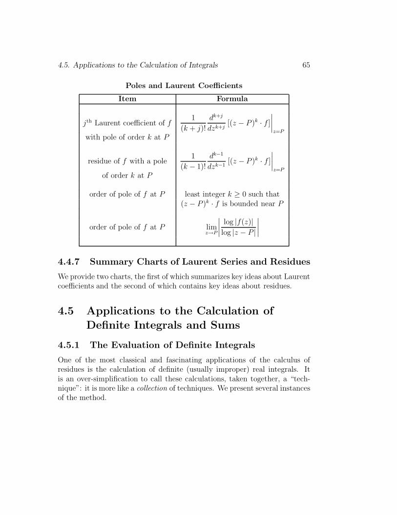
4.5. Applications to the Calculation of Integrals 65
Poles and Laurent Coefficients
Item Formula
jth Laurent coefficient of f1
(k + j)!
dk+j
dzk+j[(z − P )k · f ]
∣∣∣∣z=P
with pole of order k at P
residue of f with a pole1
(k − 1)!
dk−1
dzk−1[(z − P )k · f ]
∣∣∣∣z=P
of order k at P
order of pole of f at P least integer k ≥ 0 such that(z − P )k · f is bounded near P
order of pole of f at P limz→P
∣∣∣∣log |f(z)|log |z − P |
∣∣∣∣
4.4.7 Summary Charts of Laurent Series and Residues
We provide two charts, the first of which summarizes key ideas about Laurentcoefficients and the second of which contains key ideas about residues.
4.5 Applications to the Calculation of
Definite Integrals and Sums
4.5.1 The Evaluation of Definite Integrals
One of the most classical and fascinating applications of the calculus ofresidues is the calculation of definite (usually improper) real integrals. Itis an over-simplification to call these calculations, taken together, a “tech-nique”: it is more like a collection of techniques. We present several instancesof the method.

66 Chapter 4. Isolated Singularities
Techniques for Finding the Residue at P
Function Type of Pole Residue Calculation
f(z) simple limz→P (z − P ) · f(z)
f(z) pole of order k limz→P
µ(k−1)(z)
(k − 1)!k is the least integer suchthat limz→P µ(z) exists,
where µ(z) = (z − P )kf(z)
m(z)
n(z)m(P ) 6= 0, n(z) = 0, n′(P ) 6= 0
m(P )
n′(P )
m(z)
n(z)m has zero of order k at P (k + 1) · m(k)(P )
n(k+1)(P )n has zero of order (k + 1) at P
m(z)
n(z)m has zero of order r at P lim
z→P
µ(`−1)(z)
(`− 1)!,
n has zero of order (`+ r) at P µ(z) = (z − P )`m(z)
n(z)
4.5.2 A Basic Example of the Indefinite Integral
To evaluate ∫ ∞
−∞
1
1 + x4dx, (4.5.2.1)
we “complexify” the integrand to f(z) = 1/(1+ z4) and consider the integral
∮
γR
1
1 + z4dx.
See Figure 4.6.
Now part of the game here is to choose the right piecewise C1 curve or“contour” γR. The appropriateness of our choice is justified (after the fact)

4.5. Applications to the Calculation of Integrals 67
Figure 4.6: The integral in Subsection 4.5.2.
by the calculation that we are about to do. Assume that R > 1. Define
γ1R(t) = t+ i0 if −R ≤ t ≤ R ,
γ2R(t) = Reit if 0 ≤ t ≤ π.
Call these two curves, taken together, γ or γR.
Now we set U = C, P1 = 1/√
2 + i/√
2, P2 = −1/√
2 + i/√
2, P3 =−1/
√2− i/
√2, P4 = 1/
√2− i/
√2; the points P1, P2, P3, P4 are the poles of
1/[1 + z4]. Thus f(z) = 1/(1 + z4) is holomorphic on U \ {P1, . . . , P4} andthe Residue Theorem applies.
On the one hand,
∮
γ
1
1 + z4dz = 2πi
∑
j=1,2
Indγ(Pj) · Resf(Pj) ,
where we sum only over the poles of f that lie inside γ. These are P1 andP2. An easy calculation shows that
Resf(P1) =1
4(1/√
2 + i/√
2)3= −1
4
(1√2
+ i1√2
)
and
Resf (P2) =1
4(−1/√
2 + i/√
2)3= −1
4
(− 1√
2+ i
1√2
).
68 Chapter 4. Isolated Singularities
Of course the index at each point is 1. So
∮
γ
1
1 + z4dz = 2πi
(−1
4
)[(1√2
+ i1√2
)+
(− 1√
2+ i
1√2
)]
=π√2. (4.5.2.2)
On the other hand,∮
γ
1
1 + z4dz =
∮
γ1R
1
1 + z4dz +
∮
γ2R
1
1 + z4dz.
Trivially,
∮
γ1R
1
1 + z4dz =
∫ R
−R
1
1 + t4· 1 · dt →
∫ ∞
−∞
1
1 + t4dt (4.5.2.3)
as R → +∞. That is good, because this last is the integral that we wish toevaluate. Better still,
∣∣∣∣∣
∮
γ2R
1
1 + z4dx
∣∣∣∣∣ ≤ {length(γ2R)} · max
γ2R
∣∣∣∣1
1 + z4
∣∣∣∣ ≤ πR · 1
R4 − 1.
[Here we use the inequality |1 + z4| ≥ |z|4 − 1, as well as (2.1.7.2).] Thus
∣∣∣∣∣
∮
γ2R
1
1 + z4dz
∣∣∣∣∣→ 0 as R → ∞. (4.5.2.4)
Finally, (4.5.2.2)–(4.5.2.4) taken together yield
π√2
= limR→∞
∮
γ
1
1 + z4dz
= limR→∞
∮
γ1R
1
1 + z4dz + lim
R→∞
∮
γ2R
1
1 + z4dz
=
∫ ∞
−∞
1
1 + t4dt+ 0.
This solves the problem: the value of the integral is π/√
2.

4.5. Applications to the Calculation of Integrals 69
Figure 4.7: The integral in Subsection 4.5.3.
In other problems, it will not be so easy to pick the contour so that thesuperfluous parts (in the above example, this would be the integral over γ2
R)tend to zero, nor is it always so easy to prove that they do tend to zero.Sometimes, it is not even obvious how to complexify the integrand.
4.5.3 Complexification of the Integrand
We evaluate ∫ ∞
−∞
cos x
1 + x2dx (4.5.3.1)
by using the contour γR as in Figure 4.7 (which is the same as Figure 4.6from the previous example). The obvious choice for the complexification ofthe integrand is
f(z) =cos z
1 + z2=
[eiz + e−iz]/2
1 + z2=
[eixe−y + e−ixey]/2
1 + z2. (4.5.3.2)
Now |eixe−y| = |e−y| ≤ 1 on γR but |e−ixey| = |ey| becomes quite largeon γR when R is large and positive. There is no evident way to alter thecontour so that good estimates result. Instead, we alter the function! Letg(z) = eiz/(1 + z2).

70 Chapter 4. Isolated Singularities
On the one hand (for R > 1),
∮
γR
g(z) = 2πi · Resg(i) · IndγR(i)
= 2πi
(1
2ei
)· 1 =
π
e.
On the other hand, with γ1R(t) = t,−R ≤ t ≤ R, and γ2
R(t) = Reit, 0 ≤ t ≤ π,we have ∮
γR
g(z) dz =
∮
γ1R
g(z) dz +
∮
γ2R
g(z) dz.
Of course ∮
γ1R
g(z) dz →∫ ∞
−∞
eix
1 + x2dx as R→ ∞.
And∣∣∣∣∣
∮
γ2R
g(z) dz
∣∣∣∣∣ ≤ length(γ2R) · max
γ2R
|g| ≤ πR · 1
R2 − 1→ 0 as R → ∞.
Here we have again used (2.1.7.2).Thus
∫ ∞
−∞
cos x
1 + x2dx = Re
∫ ∞
−∞
eix
1 + x2dx = Re
(πe
)=π
e.
4.5.4 An Example with a More Subtle Choice of Con-
tour
Let us evaluate ∫ ∞
−∞
sinx
xdx. (4.5.4.1)
Before we begin, we remark that sinx/x is bounded near zero; also, theintegral converges at ∞ (as an improper Riemann integral) by integration byparts. So the problem makes sense. Using the lesson learned from the lastexample, we consider the function g(z) = eiz/z. However, the pole of eiz/z isat z = 0 and that lies on the contour in Figure 4.8. Thus that contour maynot be used. We instead use the contour µ = µR that is depicted in Figure4.9.

4.5. Applications to the Calculation of Integrals 71
Figure 4.8: The integral in Subsection 4.5.4.
Figure 4.9: More on the integral in Subsection 4.5.4.

72 Chapter 4. Isolated Singularities
Define
µ1R(t) = t, −R ≤ t ≤ −1/R,
µ2R(t) = eit/R, π ≤ t ≤ 2π,
µ3R(t) = t, 1/R ≤ t ≤ R,
µ4R(t) = Reit, 0 ≤ t ≤ π.
Clearly ∮
µ
g(z) dz =4∑
j=1
∮
µjR
g(z) dz.
On the one hand, for R > 0,∮
µ
g(z) dz = 2πiResg(0) · Indµ(0) = 2πi · 1 · 1 = 2πi. (4.5.4.2)
On the other hand,
∮
µ1R
g(z) dz +
∮
µ3R
g(z) dz →∫ ∞
−∞
eix
xdx as R→ ∞. (4.5.4.3)
Furthermore,
∣∣∣∣∣
∮
µ4R
g(z) dz
∣∣∣∣∣ ≤
∣∣∣∣∣∣∣
∮
µ4
R
Im y <√
R
g(z) dz
∣∣∣∣∣∣∣+
∣∣∣∣∣∣∣
∮
µ4
R
Im y ≥√
R
g(z) dz
∣∣∣∣∣∣∣
≡ A +B.
Now
A ≤ length(µ4R ∩ {z : Im z <
√R}) · max{|g(z)| : z ∈ µ4
R, y <√R}
≤ 4√R ·(
1
R
)→ 0 as R → ∞.
Also
B ≤ length(µ4R ∩ {z : Im z ≥
√R}) · max{|g(z)| : z ∈ µ4
R, y ≥√R}
≤ πR ·(e−
√R
R
)→ 0 as R→ ∞.

4.5. Applications to the Calculation of Integrals 73
So ∣∣∣∣∣
∮
µ4R
g(z) dz
∣∣∣∣∣→ 0 as R → ∞. (4.5.4.4)
Finally,
∮
µ2R
g(z) dz =
∫ 2π
π
ei(eit/R)
eit/R·(i
Reit)dt
= i
∫ 2π
π
ei(eit/R)dt.
As R→ ∞ this tends to
= i
∫ 2π
π
1dt
= πi as R → ∞ . (4.5.4.5)
In summary, (4.5.4.2) − (4.5.4.5) yield
2πi =
∮
µ
g(z) dz =4∑
j=1
∮
µjR
g(z) dz
→∫ ∞
−∞
eix
xdx+ πi as R→ ∞.
Taking imaginary parts yields
π =
∫ ∞
−∞
sinx
xdx.
4.5.5 Making the Spurious Part of the Integral Disap-
pear
Consider the integral ∫ ∞
0
x1/3
1 + x2dx. (4.5.5.1)
We complexify the integrand by setting f(z) = z1/3/(1 + z2). Note that,on the simply connected set U = C \ {iy : y < 0}, the expression z1/3 is
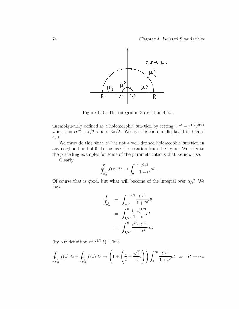
74 Chapter 4. Isolated Singularities
Figure 4.10: The integral in Subsection 4.5.5.
unambiguously defined as a holomorphic function by setting z1/3 = r1/3eiθ/3
when z = reiθ,−π/2 < θ < 3π/2. We use the contour displayed in Figure4.10.
We must do this since z1/3 is not a well-defined holomorphic function inany neighborhood of 0. Let us use the notation from the figure. We refer tothe preceding examples for some of the parametrizations that we now use.
Clearly ∮
µ3R
f(z) dz →∫ ∞
0
t1/3
1 + t2dt.
Of course that is good, but what will become of the integral over µ1R? We
have
∮
µ1R
=
∫ −1/R
−R
t1/3
1 + t2dt
=
∫ R
1/R
(−t)1/3
1 + t2dt
=
∫ R
1/R
eiπ/3t1/3
1 + t2dt.
(by our definition of z1/3 !). Thus
∮
µ3R
f(z) dz+
∮
µ1R
f(z) dz →(
1 +
(1
2+
√3
2i
))∫ ∞
0
t1/3
1 + t2dt as R→ ∞.

4.5. Applications to the Calculation of Integrals 75
On the other hand,∣∣∣∣∣
∮
µ4R
f(z) dz
∣∣∣∣∣ ≤ πR · R1/3
R2 − 1→ 0 as R → ∞
and∮
µ2R
f(z) dz =
∫ −2π
−π
(eit/R)1/3
1 + e2it/R2(i)eit/R dt
= R−4/3
∫ −2π
−π
ei4t/3
1 + e2it/R2dt → 0 as R→ ∞.
So
∮
µR
f(z) dz →(
3
2+
√3
2i
)∫ ∞
0
t1/3
1 + t2dt as R → ∞. (4.5.5.2)
The calculus of residues tells us that, for R > 1,∮
µR
f(z) dz = 2πiResf (i) · IndµR(i)
= 2πi
(eiπ/6
2i
)· 1
= π
(√3
2+i
2
). (4.5.5.3)
Finally, (4.5.5.2) and (4.5.5.3) taken together yield
∫ ∞
0
t1/3
1 + t2dt =
π√3.
4.5.6 The Use of the Logarithm
While the integral ∫ ∞
0
dx
x2 + 6x+ 8(4.5.6.1)
can be calculated using methods of calculus, it is enlightening to performthe integration by complex variable methods. Note that if we endeavor to

76 Chapter 4. Isolated Singularities
Figure 4.11: The integral in Subsection 4.5.6.
use the integrand f(z) = 1/(z2 + 6z + 8) together with the idea of the lastexample, then there is no “auxiliary radius” that helps. More precisely,((reiθ)2 + 6reiθ + 8) is a constant multiple of r2 + 6r + 8 only if θ is aninteger multiple of 2π. The following non-obvious device is often of greatutility in problems of this kind. Define log z on U ≡ C \ {x : x ≥ 0} bylog(reiθ) = (log r) + iθ when 0 < θ < 2π, r > 0. Here log r is understood tobe the standard real logarithm. Then, on U, log is a well-defined holomorphicfunction. [Observe here that there are infinitely many ways to define thelogarithm function on U . One could set log(reiθ) = (log r) + i(θ + 2kπ)for any integer choice of k. What we have done here is called “choosing abranch” of the logarithm.]
We use the contour ηR displayed in Figure 4.11 and integrate the functiong(z) = log z/(z2 + 6z + 8). Let
η1R(t) = t+ i/
√2R, 1/
√2R ≤ t ≤ R,
η2R(t) = Reit, θ0 ≤ t ≤ 2π − θ0,
where θ0(R) = tan−1(1/(R√
2R))
η3R(t) = R− t− i/
√2R, 0 ≤ t ≤ R− 1/
√2R,
η4R(t) = e−it/
√R, π/4 ≤ t ≤ 7π/4.
4.5. Applications to the Calculation of Integrals 77
Now∮
ηR
g(z) dz = 2πi(ResηR(−2) · 1 + ResηR
(−4) · 1)
= 2πi
(log(−2)
2+
log(−4)
−2
)
= 2πi
(log 2 + πi
2+
log 4 + πi
−2
)
= −πi log 2 . (4.5.6.2)
Also, it is straightforward to check that

78 Chapter 4. Isolated Singularities
∣∣∣∣∣
∮
η2R
g(z) dz
∣∣∣∣∣→ 0,
(4.5.6.3)
∣∣∣∣∣
∮
η4R
g(z) dz
∣∣∣∣∣→ 0 , (4.5.6.4)
as R → ∞. The device that makes this technique work is that, as R→ ∞,
log(x+ i/√
2R) − log(x− i/√
2R) → −2πi .
So ∮
η1R
g(z) dz +
∮
η3R
g(z) dz → −2πi
∫ ∞
0
dt
t2 + 6t+ 8. (4.5.6.5)
Now (4.5.6.2)–(4.5.6.5) taken together yield∫ ∞
0
dt
t2 + 6t+ 8=
1
2log 2.
4.5.7 Summing a Series Using Residues
We sum the series ∞∑
j=1
x
j2π2 − x2(4.5.7.1)
using contour integration. Define cot z = cos z/ sin z. For n = 1, 2, . . . letΓn be the contour (shown in Figure 4.12) consisting of the counterclockwiseoriented square with corners {(±1± i) · (n+ 1
2) · π}. For z fixed and n > |z|
we calculate using residues that
1
2πi
∮
Γn
cot ζ
ζ(ζ − z)dζ =
n∑
j=1
1
jπ(jπ − z)+
n∑
j=1
1
jπ(jπ + z)
+cot z
z− 1
z2.
When n� |z|, it is easy to estimate the left-hand side in modulus by(
1
2π
)· [4(2n + 1)π] ·
(C
n(n − |z|)
)→ 0 as n→ ∞.

4.6. SINGULARITIES AT INFINITY 79
Figure 4.12: The integral in Subsection 4.5.7.
Thus we see that
∞∑
j=1
1
jπ(jπ − z)+
∞∑
j=1
1
jπ(jπ + z)= −cot z
z+
1
z2.
We conclude that
∞∑
j=1
2
j2π2 − z2= −cot z
z+
1
z2
or∞∑
j=1
z
j2π2 − z2= −1
2cot z +
1
2z.
This is the desired result .
4.6 Singularities at Infinity
4.6.1 Meromorphic Functions
We have considered carefully those functions that are holomorphic on setsof the form D(P, r) \ {P} or, more generally, of the form U \ {P}, where Uis an open set in C and P ∈ U . As we have seen in our discussion of thecalculus of residues, sometimes it is important to consider the possibility that

80 Chapter 4. Isolated Singularities
a function could be “singular” at more than just one point. The appropriate,precise definition requires a little preliminary consideration of what kinds ofsets might be appropriate as “sets of singularities.”
4.6.2 Definition of Meromorphic Function
Now fix an open set U ; we next define the central concept of meromorphicfunction on U .
A meromorphic function f on U with singular set S is a function f :U \ S → C such that
(4.6.3.1) S is discrete;
(4.6.3.2) f is holomorphic on U \ S (note that U \ S is necessarily open inC);
(4.6.3.3) for each P ∈ S and r > 0 such that D(P, r) ⊆ U and S∩D(P, r) ={P}, the function f
∣∣D(P,r)\{P} has a (finite order) pole at P .
For convenience, one often suppresses explicit consideration of the set Sand just says that f is a meromorphic function on U . Sometimes we say,informally, that a meromorphic function on U is a function on U that isholomorphic “except for poles.” Implicit in this description is the idea thata pole is an “isolated singularity.” In other words, a point P is a pole of f ifand only if there is a disc D(P, r) around P such that f is holomorphic onD(P, r) \ {P} and has a pole at P . Back on the level of precise language,we see that our definition of a meromorphic function on U implies that, foreach P ∈ U, either there is a disc D(P, r) ⊆ U such that f is holomorphicon D(P, r) or there is a disc D(P, r) ⊆ U such that f is holomorphic onD(P, r) \ {P} and has a pole at P .
4.6.3 Examples of Meromorphic Functions
Meromorphic functions are very natural objects to consider, primarily be-cause they result from considering the (algebraic) reciprocals—or more gen-erally the quotients—of holomorphic functions:
If U is a connected, open set in C and if f : U → C is a holomorphicfunction having at least some zeros but with f 6≡ 0, then the function
F : U \ {z : f(z) = 0} → C (4.6.4.1)

4.6. SINGULARITIES AT INFINITY 81
defined by F (z) = 1/f(z) is a meromorphic function on U with singular set(or pole set) equal to {z ∈ U : f(z) = 0}. More generally, meromorphicfunctions locally have the form g(z)/f(z) for f, g holomorphic. In a sensethat can be made precise, all meromorphic functions arise as quotients ofholomorphic functions.
4.6.4 Meromorphic Functions with Infinitely Many Poles
It is quite possible for a meromorphic function on an open set U to haveinfinitely many poles in U . The function 1/ sin(1/z) is an obvious exampleon U = D \ {0}.
4.6.5 Singularities at Infinity
Our discussion so far of singularities of holomorphic functions can be gener-alized to include the limit behavior of holomorphic functions as |z| → +∞.This is a powerful method with many important consequences. Suppose forexample that f : C → C is an entire function. We can associate to f anew function G : C \ {0} → C by setting G(z) = f(1/z). The behaviorof the function G near 0 reflects, in an obvious sense, the behavior of f as|z| → +∞. For instance
lim|z|→+∞
|f(z)| = +∞ (4.6.6.1)
if and only if G has a pole at 0.
Suppose that f : U → C is a holomorphic function on an open set U ⊆ C
and that, for some R > 0, U ⊇ {z : |z| > R}. Define G : {z : 0 < |z| <1/R} → C by G(z) = f(1/z). Then we say that
(4.6.6.2) f has a removable singularity at ∞ ifG has a removable singularityat 0.
(4.6.6.3) f has a pole at ∞ if G has a pole at 0.
(4.6.6.4) f has an essential singularity at ∞ if G has an essential singularityat 0.

82 Chapter 4. Isolated Singularities
4.6.6 The Laurent Expansion at Infinity
The Laurent expansion of G around 0, G(z) =∑+∞
−∞ anzn, yields immediately
a series expansion for f which converges for |z| > R, namely,
f(z) ≡ G(1/z) =+∞∑
−∞anz
−n =+∞∑
−∞a−nz
n. (4.6.7.1)
The series∑+∞
−∞ a−nzn is called the Laurent expansion of f around ∞.
It follows from our definitions and from our earlier discussions that f has aremovable singularity at ∞ if and only if the Laurent series of f at ∞ hasno positive powers of z with non-zero coefficients. Also f has a pole at ∞ ifand only if the series has only a finite number of positive powers of z withnon-zero coefficients. Finally, f has an essential singularity at ∞ if and onlyif the series has infinitely many positive powers.
4.6.7 Meromorphic at Infinity
Suppose that f : C → C is an entire function. Then lim|z|→+∞ |f(z)| = +∞ ifand only if f is a nonconstant polynomial. In other words, an entire functionthat is not a polynomial will have an essential singularity at infinity.
To see this last assertion, supposed that f has a pole of order k at ∞.Subtracting a polynomial p from f if necessary, we may arrange that f − pvanishes to order k at the origin. Of course p has degree at most k. Thenthe function
g(z) =f(z) − p(z)
zk
is entire and is bounded. By Liouville’s theorem, g is constant. But then itfollows that f is a polynomial.
The entire function f has a removable singularity at ∞ if and only if fis a constant. This claim if obvious because f will be bounded.
Suppose that f is a meromorphic function defined on an open set U ⊆ C
such that, for some R > 0, we have U ⊇ {z : |z| > R}. We say that fis meromorphic at ∞ if the function G(z) ≡ f(1/z) is meromorphic in theusual sense on {z : |z| < 1/R}.

4.6. SINGULARITIES AT INFINITY 83
4.6.8 Meromorphic Functions in the Extended
Plane
The definition of “meromorphic at ∞” as given is equivalent to requiringthat, for some R′ > R, f has no poles in {z ∈ C : R′ < |z| < ∞} and thatf has a pole at ∞. The point is that a pole should not be an accumulationpoint of other poles.
A meromorphic function f on C which is also meromorphic at ∞ mustbe a rational function (that is, a quotient of polynomials in z). For we canarrange for one of the poles to be at ∞. Multiplying f by a polynomial p, wemay arrange for p ·f to have no poles. So it must be a polynomial. It followsthat f is a quotient of polynomials. Conversely, every rational function ismeromorphic on C and at ∞.
Remark: It is conventional to rephrase the ideas just presented by sayingthat the only functions that are meromorphic in the “extended plane” arerational functions. We will say more about the extended plane in §§6.3.1–6.3.3.


Chapter 5
The Argument Principle
5.1 Counting Zeros and Poles
5.1.1 Local Geometric Behavior of a Holomorphic
Function
In this chapter, we shall be concerned with questions that have a geometric,qualitative nature rather than an analytical, quantitative one. These ques-tions center around the issue of the local geometric behavior of a holomorphicfunction.
5.1.2 Locating the Zeros of a Holomorphic Function
Suppose that f : U → C is a holomorphic function on a connected, open setU ⊆ C and that D(P, r) ⊆ U . We know from the Cauchy integral formulathat the values of f on D(P, r) are completely determined by the values of fon ∂D(P, r). In particular, the number and even the location of the zeros of finD(P, r) are determined in principle by f on ∂D(P, r). But it is nonethelessa pleasant surprise that there is a simple formula for the number of zeros off in D(P, r) in terms of f (and f ′) on ∂D(P, r). In order to obtain a preciseformula, we shall have to agree to count zeros according to multiplicity (see§§3.1.4). We now explain the precise idea.
Let f : U → C be holomorphic as before, and assume that f has somezeros in U but that f is not identically zero. Fix z0 ∈ U such that f(z0) = 0.Since the zeros of f are isolated, there is an r > 0 such that D(z0, r) ⊆ Uand such that f does not vanish on D(z0, r) \ {z0}.
85

86 CHAPTER 5. THE ARGUMENT PRINCIPLE
Now the power series expansion of f about z0 has a first non-zero termdetermined by the least positive integer n such that f (n)(z0) 6= 0. (Note thatn ≥ 1 since f(z0) = 0 by hypothesis.) Thus the power series expansion of fabout z0 begins with the nth term:
f(z) =
∞∑
j=n
1
j!
∂jf
∂zj(z0)(z − z0)
j . (5.1.2.1)
Under these circumstances we say that f has a zero of order n (or multiplicityn) at z0. When n = 1, then we also say that z0 is a simple zero of f .
5.1.3 Zero of Order n
The concept of zero of “order n,” or “multiplicity n,” for a function f is soimportant that a variety of terminology has grown up around it (see also§§3.1.4). It has already been noted that, when the multiplicity n = 1, thenthe zero is sometimes called simple. For arbitrary n, we sometimes say that“n is the order of z0 as a zero of f .” More generally if f(z0) = β so that, forsome n ≥ 1, the function f( · ) − β has a zero of order n at z0, then we sayeither that “f assumes the value β at z0 to order n” or that “the order ofthe value β at z0 is n.” When n > 1, then we call z0 a multiple point (and βa multiple value) of the function f .
The next result provides a method for computing the multiplicity n ofthe zero at z0 from the values of f, f ′ on the boundary of a disc centered atz0.
5.1.4 Counting the Zeros of a Holomorphic Function
If f is holomorphic on a neighborhood of a disc D(P, r) and has a zero oforder n at P and no other zeros in the closed disc, then
1
2πi
∮
∂D(P,r)
f ′(ζ)
f(ζ)dζ = n. (5.1.4.1)
More generally, we consider the case that f has several zeros—with dif-ferent locations and different multiplicities—inside a disc: Suppose thatf : U → C is holomorphic on an open set U ⊆ C and that D(P, r) ⊆ U .Suppose that f is non-vanishing on ∂D(P, r) and that z1, z2, . . . , zk are the

5.1. COUNTING ZEROS AND POLES 87
Figure 5.1: Counting the zeros of a holomorphic function.
zeros of f in the interior of the disc. Let n` be the order of the zero of f atz`, ` = 1, . . . , k. Then
1
2π
∮
|ζ−P |=r
f ′(ζ)
f(ζ)dζ =
k∑
`=1
n`. (5.1.4.2)
Refer to Figure 5.1 for illustrations of both these situations.The reasons for these formulas is actually quite simple. The primordial
situation is when P = 0 and f(z) = zk. In that case we may compute theintegral (5.1.4.1) directly and the result is immediate. We may write a more
general f as f(z) = f(z)·zk and then the integral (5.1.4.1) reduces, by simplealgebra, to the simpler situation just treated. Of course the integral over amore general curve can be reduced to the integral over the boundary of a discby our usual device of deformation of curves. Finally, the situation of severaldifferent zeros may be reduced to the situation of one zero by breaking upthe curve of integration into smaller curves, each having just one zero in itsinterior.
5.1.5 The Argument Principle
This last formula (5.1.4.2), which is often called the argument principle, isboth useful and important. For one thing, there is no obvious reason why
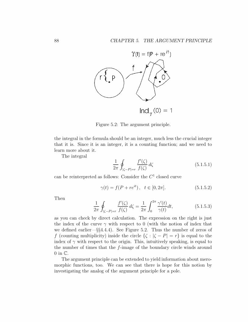
88 CHAPTER 5. THE ARGUMENT PRINCIPLE
Figure 5.2: The argument principle.
the integral in the formula should be an integer, much less the crucial integerthat it is. Since it is an integer, it is a counting function; and we need tolearn more about it.
The integral1
2π
∮
|ζ−P |=r
f ′(ζ)
f(ζ)dζ (5.1.5.1)
can be reinterpreted as follows: Consider the C1 closed curve
γ(t) = f(P + reit) , t ∈ [0, 2π]. (5.1.5.2)
Then1
2π
∮
|ζ−P |=r
f ′(ζ)
f(ζ)dζ =
1
2π
∫ 2π
0
γ′(t)
γ(t)dt, (5.1.5.3)
as you can check by direct calculation. The expression on the right is justthe index of the curve γ with respect to 0 (with the notion of index thatwe defined earlier—§§4.4.4). See Figure 5.2. Thus the number of zeros off (counting multiplicity) inside the circle {ζ : |ζ − P | = r} is equal to theindex of γ with respect to the origin. This, intuitively speaking, is equal tothe number of times that the f -image of the boundary circle winds around0 in C.
The argument principle can be extended to yield information about mero-morphic functions, too. We can see that there is hope for this notion byinvestigating the analog of the argument principle for a pole.
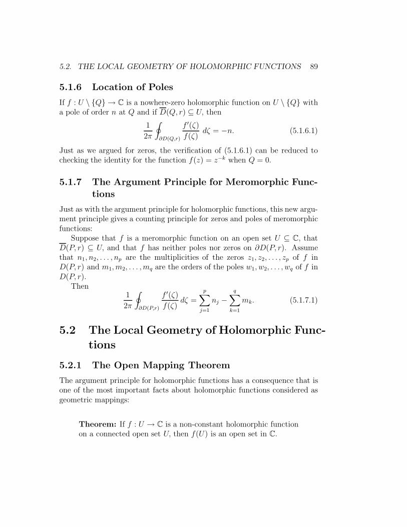
5.2. THE LOCAL GEOMETRY OF HOLOMORPHIC FUNCTIONS 89
5.1.6 Location of Poles
If f : U \ {Q} → C is a nowhere-zero holomorphic function on U \ {Q} witha pole of order n at Q and if D(Q, r) ⊆ U, then
1
2π
∮
∂D(Q,r)
f ′(ζ)
f(ζ)dζ = −n. (5.1.6.1)
Just as we argued for zeros, the verification of (5.1.6.1) can be reduced tochecking the identity for the function f(z) = z−k when Q = 0.
5.1.7 The Argument Principle for Meromorphic Func-
tions
Just as with the argument principle for holomorphic functions, this new argu-ment principle gives a counting principle for zeros and poles of meromorphicfunctions:
Suppose that f is a meromorphic function on an open set U ⊆ C, thatD(P, r) ⊆ U, and that f has neither poles nor zeros on ∂D(P, r). Assumethat n1, n2, . . . , np are the multiplicities of the zeros z1, z2, . . . , zp of f inD(P, r) and m1, m2, . . . , mq are the orders of the poles w1, w2, . . . , wq of f inD(P, r).
Then1
2π
∮
∂D(P,r)
f ′(ζ)
f(ζ)dζ =
p∑
j=1
nj −q∑
k=1
mk. (5.1.7.1)
5.2 The Local Geometry of Holomorphic Func-
tions
5.2.1 The Open Mapping Theorem
The argument principle for holomorphic functions has a consequence that isone of the most important facts about holomorphic functions considered asgeometric mappings:
Theorem: If f : U → C is a non-constant holomorphic functionon a connected open set U, then f(U) is an open set in C.
90 CHAPTER 5. THE ARGUMENT PRINCIPLE
Figure 5.3: The open mapping principle.
(5.2.1.1)
See Figure 5.3. The result says, in particular, that if U ⊆ C is connectedand open and if f : U → C is holomorphic, then either f(U) is a connectedopen set (the non-constant case) or f(U) is a single point.
To see why the open mapping principle is true, let β be a value of theholomorphic function f . Say that f(b) = β, and let D(b, r) be a small discas usual in the domain of f . Suppose for simplicity that β is a simple valueof f . Then of course
1 =1
2πi
∮
∂D(b,r)
f ′(ζ)
f(ζ) − βdζ . (5.2.1.2)
If we perturb β a little bit on the righthand side of this integral (a perturba-tion much smaller than r), then the integral will still be integer-valued, andits value will be very close to 1. So in fact it must be 1. Thus we concludethat f also takes on that small perturbed value of β. We have argued thenthat f assumes all values near β. But this means that the image of f is open.
In the subject of topology, a function f is defined to be continuous if theinverse image of any open set under f is also open. In contexts where theε− δ definition makes sense, the ε− δ definition (§§2.2.1, 2.2.2) is equivalentto the inverse-image-of-open-sets definition. By contrast, functions for whichthe direct image of any open set is open are called “open mappings.”
Here is a quantitative, or counting, statement that comes from the proofof the open mapping principle: Suppose that f : U → C is a non-constant
5.3. Further Results on Zeros 91
holomorphic function on a connected open set U such that P ∈ U andf(P ) = Q with order k. Then there are numbers δ, ε > 0 such that eachq ∈ D(Q, ε) \ {Q} has exactly k distinct pre-images in D(P, δ) and eachpre-image is a simple point of f . Of course the justification is again a simpleapplication of (5.2.1.2).
The considerations that establish the open mapping principle can alsobe used to establish the fact that if f : U → V is a one-to-one and ontoholomorphic function, then f−1 : V → U is also holomorphic.
5.3 Further Results on the Zeros of Holomor-
phic Functions
5.3.1 Rouche’s Theorem
Now we consider global aspects of the argument principle.Suppose that f, g : U → C are holomorphic functions on an open set
U ⊆ C. Suppose also that D(P, r) ⊆ U and that, for each ζ ∈ ∂D(P, r),
|f(ζ) − g(ζ)| < |f(ζ)| + |g(ζ)|. (5.3.1.1)
Then1
2π
∮
∂D(P,r)
f ′(ζ)
f(ζ)dζ =
1
2π
∮
∂D(P,r)
g′(ζ)
g(ζ)dζ. (5.3.1.2)
That is, the number of zeros of f in D(P, r) counting multiplicities equalsthe number of zeros of g in D(P, r) counting multiplicities.
Remark: Rouche’s theorem is often stated with the stronger hypothesis that
|f(ζ) − g(ζ)| < |g(ζ)| (5.3.1.3)
for ζ ∈ ∂D(P, r). Rewriting this hypothesis as
∣∣∣∣f(ζ)
g(ζ)− 1
∣∣∣∣ < 1, (5.3.1.4)
we see that it says that the image γ under f/g of the circle ∂D(P, r) lies inthe disc D(1, 1). See Figure 5.4. Our weaker hypothesis that |f(ζ)− g(ζ)| <|f(ζ)|+ |g(ζ)| has the geometric interpretation that f(ζ)/g(ζ) lies in the set

92 CHAPTER 5. THE ARGUMENT PRINCIPLE
Figure 5.4: Rouche’s theorem.
C \ {x + i0 : x ≤ 0}. Either hypothesis implies that the image of the circle∂D(P, r) under f has the same “winding number” around 0 as does the imageunder g of that circle.
5.3.2 Typical Application of Rouche’s Theorem
EXAMPLE 5.3.2.1 Let us determine the number of roots of the polyno-mial f(z) = z7 + 5z3 − z − 2 in the unit disc. We do so by comparing thefunction f to the holomorphic function g(z) = 5z3 on the unit circle. For|z| = 1 we have
|f(z) − g(z)| = |z7 − z − 2| ≤ 4 < |g(ζ)| ≤ |f(ζ)| + |g(ζ)|.By Rouche’s theorem, f and g have the same number of zeros, countingmultiplicity, in the unit disc. Since g has three zeros, so does f .
5.3.3 Rouche’s Theorem and the Fundamental Theo-
rem of Algebra
Rouche’s theorem provides a useful way to locate approximately the zerosof a holomorphic function that is too complicated for the zeros to be ob-tained explicitly. As an illustration, we analyze the zeros of a non-constantpolynomial
P (z) = zn + an−1zn−1 + an−2z
n−2 + · · · + a1z + a0. (5.3.3.1)

5.4. THE MAXIMUM PRINCIPLE 93
If R is sufficiently large (say R > max{1, n · max0≤j≤n−1 |aj|
}) and |z| = R,
then|an−1z
n−1 + an−2zn−2 + · · · + a0|
|zn| < 1. (5.3.3.2)
Thus Rouche’s theorem applies on D(0, R) with f(z) = zn and g(z) = P (z).We conclude that the number of zeros of P (z) inside D(0, R), counting mul-tiplicities, is the same as the number of zeros of zn inside D(0, R), countingmultiplicities—namely n. Thus we recover the Fundamental Theorem of Al-gebra. Incidentally, this example underlines the importance of counting zeroswith multiplicities: the function zn has only one root in the naıve sense ofcounting the number of points where it is zero; but it has n roots when theyare counted with multiplicity.
5.3.4 Hurwitz’s Theorem
A second useful consequence of the argument principle is the following resultabout the limit of a sequence of zero-free holomorphic functions:
Hurwitz’s theorem Suppose that U ⊆ C is a connected openset and that {fj} is a sequence of nowhere-vanishing holomorphicfunctions on U . If the sequence {fj} converges uniformly on com-pact subsets of U to a (necessarily holomorphic) limit functionf0, then either f0 is nowhere-vanishing or f0 ≡ 0.
We leave the proof to the reader: Examine the integral
1
2πi
∮
∂D(P,r)
f ′j(ζ)
fj(ζ)dζ
for a suitable disc in the common domain of the functions in question.
5.4 The Maximum Principle
5.4.1 The Maximum Modulus Principle
We repeat that a domain in C is a connected open set (§§1.3.1). A boundeddomain is a connected open set U such that there is an R > 0 with |z| < Rfor all z ∈ U—or U ⊆ D(0, R).

94 CHAPTER 5. THE ARGUMENT PRINCIPLE
The Maximum Modulus Principle
Theorem: Let U ⊆ C be a domain. Let f be a holomorphicfunction on U . If there is a point P ∈ U such that |f(P )| ≥ |f(z)|for all z ∈ U , then f is constant.
Here is a sharper variant of the theorem:
Theorem: Let U ⊆ C be a domain and let f be a holomorphicfunction on U . If there is a point P ∈ U at which |f | has a localmaximum, then f is constant.
There are a variety of ways to prove the maximum principle. A standardmethod is to first establish this mean value property: If f is holomorphic ina neighborhood of D(P, r) then
f(P ) =1
2π
∫ 2π
0
f(P + reit) dt .
One establishes this formula by first taking P = 0 and checking the result forthe case f(z) = zk, any k ≥ 0. Then one extends to an arbitrary holomorphicfunction by using power series.
Now to establish the maximum principle, assume that f is not constantas asserted. Let E be the set on which |f | assumes its maximum value|f(P )| ≡ λ. Let w be a point of E that is nearest to ∂U . If r > 0 is a smallnumber then
λ = |f(w)| =1
2π
∣∣∣∣∫ 2π
0
f(w + reit) dt
∣∣∣∣ ≤1
2π
∫ 2π
0
|f(w + reit)| dt .
Now because w is an extreme point of E, it is not the case that w+ reit liesin E for all values of t. As a result, |f(w + reit)| < λ for t in an open arc of[0, 2π]. Thus we may conclude that the last line is
<1
2π
∫ 2π
0
λdt = λ .
We conclude that λ < λ, and that is a contradiction.We leave the details of the sharper version of the maximum principle for
the interested reader.

5.4. THE MAXIMUM PRINCIPLE 95
5.4.2 Boundary Maximum Modulus Theorem
The following version of the maximum principle is intuitively appealing, andis frequently useful.
Theorem: Let U ⊆ C be a bounded domain. Let f be a con-tinuous function on U that is holomorphic on U . Then the max-imum value of |f | on U (which must occur, since U is closed andbounded—see [RUD1], [KRA3]) must in fact occur on ∂U .
In other words,
maxU
|f | = max∂U
|f |.
The proof is straightforward and we omit it.
5.4.3 The Minimum Principle
Holomorphic functions (or, more precisely, their moduli) can have interiorminima. The function f(z) = z2 on D(0, 1) has the property that z = 0 isa global minimum for |f |. However, it is not accidental that this minimumvalue is 0:
Theorem: Let f be holomorphic on a domain U ⊆ C. As-sume that f never vanishes. If there is a point P ∈ U such that|f(P )| ≤ |f(z)| for all z ∈ U , then f is constant. This result isproved by applying the maximum principle to the function 1/f .
There is also a boundary minimum principle:
Theorem: Let U ⊆ C be a bounded domain. Let f be a con-tinuous function on U that is holomorphic on U . Assume thatf never vanishes on U . Then the minimum value of |f | on U(which must occur, since U is closed and bounded—see [RUD1],[KRA3]) must occur on ∂U .
In other words,
minU
|f | = min∂U
|f |.

96 CHAPTER 5. THE ARGUMENT PRINCIPLE
5.4.4 The Maximum Principle on an Unbounded Do-
main
It should be noted that the boundary maximum modulus theorem is notalways true on an unbounded domain. The standard example is the functionf(z) = exp(exp(z)) on the domain U = {z = x + iy : −π/2 < y < π/2}.Check for yourself that |f | = 1 on the boundary of U . But the restrictionof f to the real number line is unbounded at infinity. The theorem does,however, remain true with some additional restrictions. The result, knownas the Phragmen-Lindelof theorem,1 is one method of treating maximummodulus theorems on unbounded domains (see [RUD2]).
5.5 The Schwarz Lemma
This section treats certain estimates that bounded holomorphic functions onthe unit disc necessarily satisfy. We present the classical, analytic viewpointin the subject (instead of the geometric viewpoint—see [KRA2]).
5.5.1 Schwarz’s Lemma
Theorem: Let f be holomorphic on the unit disc. Assume that
(5.5.1.1) |f(z)| ≤ 1 for all z.
(5.5.1.2) f(0) = 0.
Then |f(z)| ≤ |z| and |f ′(0)| ≤ 1.
If either |f(z)| = |z| for some z 6= 0 or if |f ′(0)| = 1, then fis a rotation: f(z) ≡ αz for some complex constant α of unitmodulus.
For the proof, consider the function g(z) = f(z)/z. This function is holo-morphic and is still bounded by 1 as |z| → 1. The result then follows fromthe maximum principle.
Schwarz’s lemma is a profound geometric fact that has exerted consid-erable influence in the subject. We cannot explore these avenues here, but
1This theorem imposes a Tauberian hypothesis on the function to make up for the fact
that the domain is unbounded.

5.5. THE SCHWARZ LEMMA 97
see [KRA2]. One nice application is that the lemma enables one to clas-sify the invertible holomorphic self-maps of the unit disc (see [GK]). (Herea self-map of a domain U is a mapping F : U → U of the domain to it-self.) These are commonly referred to as the “conformal self-maps” of thedisc. The classification is as follows: If 0 ≤ θ < 2π, then define the rotationthrough angle θ to be the function ρθ(z) = eiθz; if a is a complex numberof modulus less than one, then define the associated Mobius transformationto be ϕa(z) = [z − a]/[1 − az]. Any conformal self-map of the disc is thecomposition of some rotation ρθ with some Mobius transformation ϕa. Thistopic is treated in detail in §6.2.
The classification works as follows. Let ψ be a conformal self-map of thedisc D. Suppose that ψ(0) = a. Then consider h = ϕa ◦ ψ. We see thath : D → D and h(0) = 0. Thus the Schwarz lemma applies and |h(z)| ≤ |z|.The same reasoning applies to h−1 so that |h(z)| ≥ |z|. We conclude that|h(z)| = |z| so that h is a rotation. The result follows.
We conclude this section by presenting a generalization of the Schwarzlemma, in which we consider holomorphic mappings f : D → D, but wediscard the hypothesis that f(0) = 0. This result is known as the Schwarz-Pick lemma.
5.5.2 The Schwarz-Pick Lemma
Theorem: Let f be holomorphic on the unit disc. Assume that
(5.5.2.1) |f(z)| ≤ 1 for all z.
(5.5.2.2) f(a) = b for some a, b ∈ D(0, 1).
Then
|f ′(a)| ≤ 1 − |b|21 − |a|2 . (5.5.2.3)
Moreover, if f(a1) = b1 and f(a2) = b2, then
∣∣∣∣b2 − b1
1 − b1b2
∣∣∣∣ ≤∣∣∣∣a2 − a1
1 − a1a2
∣∣∣∣ . (5.5.2.4)

98 CHAPTER 5. THE ARGUMENT PRINCIPLE
There is a “uniqueness” result in the Schwarz-Pick Lemma. If either
|f ′(a)| =1 − |b|21 − |a|2 or
∣∣∣∣b2 − b1
1 − b1b2
∣∣∣∣ =∣∣∣∣a2 − a1
1 − a1a2
∣∣∣∣ with a1 6= a2 ,
(5.5.2.5)then the function f is a conformal self-mapping (one-to-one, onto holomor-phic function) of D(0, 1) to itself.
The proof of Schwarz-Pick is nearly obvious. Consider h = ϕb ◦ f ◦ ϕ−a.Then h : D → D, h(0) = 0, and the Schwarz lemma applies.


100 CHAPTER 5. THE ARGUMENT PRINCIPLE
Chapter 6
The Geometric Theory ofHolomorphic Functions
6.1 The Idea of a Conformal Mapping
6.1.1 Conformal Mappings
The main objects of study in this chapter are holomorphic functions h : U →V, with U and V open in C, that are one-to-one and onto. Such a holomorphicfunction is called a conformal (or biholomorphic) mapping. The fact that his supposed to be one-to-one implies that h′ is nowhere zero on U [rememberthat if h′ vanishes to order k ≥ 0 at a point P ∈ U , then h is (k + 1)-to-1in a small neighborhood of P—see §§5.2.1]. As a result, h−1 : V → U is alsoholomorphic—as we discussed in §§5.2.1. A conformal map h : U → V fromone open set to another can be used to transfer holomorphic functions on Uto V and vice versa: that is, f : V → C is holomorphic if and only if f ◦ his holomorphic on U ; and g : U → C is holomorphic if and only if g ◦ h−1 isholomorphic on V .
Thus, if there is a conformal mapping from U to V, then U and V areessentially indistinguishable from the viewpoint of complex function theory.On a practical level, one can often study holomorphic functions on a rathercomplicated open set by first mapping that open set to some simpler openset, then transferring the holomorphic functions as indicated.
101

102 Chapter 6. Geometric Theory of Holomorphic Functions
6.1.2 Conformal Self-Maps of the Plane
The simplest open subset of C is C itself. Thus it is natural to begin ourstudy of conformal mappings by considering the conformal mappings of C toitself. In fact the conformal mappings from C to C can be explicitly describedas follows:
Theorem: A function f : C → C is a conformal mapping if andonly if there are complex numbers a, b with a 6= 0 such that
f(z) = az + b , z ∈ C. (6.1.2.1)
One aspect of the result is fairly obvious: If a, b ∈ C and a 6= 0, then themap z 7→ az + b is certainly a conformal mapping of C to C. In fact onechecks easily that z 7→ (z− b)/a is the inverse mapping. The interesting partof the assertion is that these are in fact the only conformal maps of C to C.
For the proof, note that the holomorphic function f satisfies
lim|z|→+∞
|f(z)| = +∞.
That is, given ε > 0, there is a number C > 0 such that if |z| > C then|f(z)| > 1/ε. The set {z : |z| ≤ 1/ε} is a compact subset of C. Since f−1 :C → C is holomorphic, it is continuous. And the continuous image of acompact set is compact. Therefore S = f−1
({z : |z| ≤ 1/ε}
)is compact.
By the Heine-Borel theorem, S must be bounded. Thus there is a positivenumber C such that S ⊆ {z : |z| ≤ C}.
Taking contrapositives, we see that if |w| > C then w is not an elementof f−1
({z : |z| ≤ 1/ε}
). Therefore f(w) is not an element of {z : |z| ≤ 1/ε}.
In other words, |f(w)| > 1/ε. That is the desired result.Further understanding of the behavior of f(z) when z has large absolute
value may be obtained by applying the technique already used in Chapter4 to talk about singularities at ∞. Define, for all z ∈ C such that z 6= 0and f(1/z) 6= 0, a function g(z) = 1/f(1/z). By Lemma x.y.z, there is anumber C such that |f(z)| > 1 if |z| > C. Clearly g is defined on {z : 0 <|z| < 1/C}. Furthermore, g is bounded on this set by 1. By the Riemannremovable singularities theorem, g extends to be holomorphic on the full discD(0, 1/C) = {z : |z| < 1/C}. Lemma x.y.z tells us that in fact g(0) = 0.

6.1. The Idea of a Conformal Mapping 103
Now, because f : C → C is one-to-one, it follows that g is one-to-one onthe disc D(0, 1/C). In particular, g′(0) cannot be 0. Since
0 6= |g′(0)| = lim|z|→0+
∣∣∣∣g(z) − g(0)
z
∣∣∣∣ = lim|z|→0+
∣∣∣∣g(z)
z
∣∣∣∣ ,
we see that there is a constant A > 0 such that
|g(z)| ≥ A|z|
for z sufficiently small. We next translate this to information about theoriginal function f.
Now we claim that there are numbers B,D > 0 such that, if |z| > D,then
|f(z)| < B|z| .To see this, as noted above, there is a number δ > 0 such that if |z| < δ then|g(z)| ≥ A|z|. If |z| > 1/δ then
|f(z)| =1
|g(1/z)| ≤1
A|1/z| =1
A|z|.
Thus the lemma holds with B = 1/A and D = 1/δ.The proof of our main result is now easily given. By (6.1.2.1), f is a
polynomial of degree at most 1, i.e. f(z) = az+ b for some a, b ∈ C. Clearlyf is one-to-one and onto if and only if a 6= 0. That proves the result.
One part of the proof just given is worth considering in the more generalcontext of singularities at ∞, as discussed in Section 4.7. Suppose now thath is holomorphic on a set {z : |z| > α}, for some positive α, and that
lim|z|→+∞
|h(z)| = +∞.
Then it remains true that g(z) ≡ 1/h(1/z) is defined and holomorphic on{z : 0 < |z| < η}, some η > 0. Also, by the same reasoning as above, gextends holomorphically to D(0, η) with g(0) = 0. If we do not assume inadvance that h is one-to-one then we may not say (as we did before) thatg′(0) 6= 0. But g is not constant, since h is not, so there is a positive integern and a positive number A such that
|g(z)| ≥ A|z|n
104 Chapter 6. Geometric Theory of Holomorphic Functions
for all z with |z| sufficiently small. It then follows (as in the proof of Lemma6.1.2) that
|h(z)| ≤ 1
A|z|n
for |z| sufficiently large. This line of reasoning, combined with Theorem 3.4.4,recovers Theorem 4.7.6: If h : C → C is a holomorphic function such that
lim|z|→+∞
|h(z)| = +∞,
then h is a polynomial.A generalization of this result about conformal maps of the plane is the
following (consult §§4.6.8 as well as the detailed explanation in [GRK]):
If h : C → C is a holomorphic function such that
lim|z|→+∞
|h(z)| = +∞,
then h is a polynomial.
We in fact treated this result, using slightly different terminology, whenwe discussed isolated singularities at infinity.
6.2 Linear Fractional Transformations
6.2.1 Linear Fractional Mappings
The automorphisms (that is, conformal self-mappings) of the unit disc D arespecial cases of functions of the form
z 7→ az + b
cz + d, a, b, c, d ∈ C. (6.3.1.1)
It is worthwhile to consider functions of this form in generality. One restric-tion on this generality needs to be imposed, however; if ad − bc = 0, thenthe numerator is a constant multiple of the denominator provided that thedenominator is not identically zero. So if ad − bc = 0, then the function iseither constant or has zero denominator and is nowhere defined. Thus onlythe case ad− bc 6= 0 is worth considering in detail.

6.3. Linear Fractional Transformations 105
A function of the form
z 7→ az + b
cz + d, ad− bc 6= 0, (6.3.1.2)
is called a linear fractional transformation.
Note that (az + b)/(cz + d) is not necessarily defined for all z ∈ C.Specifically, if c 6= 0, then it is undefined at z = −d/c. In case c 6= 0,
limz→−d/c
∣∣∣∣az + b
cz + d
∣∣∣∣ = +∞. (6.3.1.3)
This observation suggests that one might well, for linguistic convenience,adjoin formally a “point at ∞” to C and consider the value of (az+b)/(cz+d)to be ∞ when z = −d/c (c 6= 0). Thus we will think of both the domainand the range of our linear fractional transformation to be C ∪ {∞} (we
sometimes also use the notation C instead of C ∪ {∞}). Specifically, weare led to the following alternative method for describing a linear fractionaltransformation.
A function f : C ∪ {∞} → C ∪ {∞} is a linear fractional transformationif there exists a, b, c, d ∈ C, ad− bc 6= 0, such that either
(6.3.1.4) c = 0, d 6= 0, f(∞) = ∞, and f(z) = (a/d)z + (b/d) for all z ∈ C;
or
(6.3.1.5) c 6= 0, f(∞) = a/c, f(−d/c) = ∞, and f(z) = (az + b)/(cz + d)for all z ∈ C, z 6= −d/c.
It is important to realize that, as before, the status of the point ∞ isentirely formal: we are just using it as a linguistic convenience, to keep trackof the behavior of f(z) both where it is not defined as a map on C and to keeptrack of its behavior when |z| → +∞. The justification for the particulardevices used is the fact that
(6.3.1.6) lim|z|→+∞ f(z) = f(∞) [c = 0; case (6.3.1.4) of the definition]
(6.3.1.7) limz→−d/c |f(z)| = +∞ [c 6= 0; case (6.3.1.5) of the definition].

106 Chapter 6. Geometric Theory of Holomorphic Functions
6.2.2 The Topology of the Extended Plane
The limit properties of f that we described in §§6.3.1 can be considered ascontinuity properties of f from C ∪ {∞} to C ∪ {∞} using the definition ofcontinuity that comes from the topology on C∪{∞}. It is easy to formulatethat topology in terms of open sets. But it is also convenient to formulatethat same topological structure in terms of convergence of sequences:
A sequence {pi} in C ∪ {∞} converges to p0 ∈ C ∪ {∞} (notationlimi→∞ pi = p0) if either
(6.3.2.1) p0 = ∞ and limi→+∞ |pi| = +∞ where the limit is taken for all isuch that pi ∈ C;
or
(6.3.2.2) p0 ∈ C, all but a finite number of the pi are in C and limi→∞ pi = p0
in the usual sense of convergence in C.
6.2.3 The Riemann Sphere
Stereographic projection puts C = C ∪ {∞} into one-to-one correspondencewith the two-dimensional sphere S in R3, S = {(x, y, z) ∈ R3 : x2 + y2 +z2 = 1} in such a way that topology is preserved in both directions of thecorrespondence.
In detail, begin by imagining the unit sphere bisected by the complexplane with the center of the sphere (0, 0, 0) coinciding with the origin in theplane—see Figure 6.1. We define the stereographic projection as follows: IfP = (x, y) ∈ C, then connect P to the “north pole” N of the sphere with aline segment. The point π(P ) of intersection of this segment with the sphereis called the stereographic projection of P . Note that, under stereographicprojection, the “point at infinity” in the plane corresponds to the north poleN of the sphere. For this reason, C ∪ {∞} is often thought of as “being” asphere, and is then called, for historical reasons, the Riemann sphere.
The construction we have just described is another way to think aboutthe “extended complex plane”—see §§6.3.2. In these terms, linear fractionaltransformations become homeomorphisms of C ∪ {∞} to itself. (Recall thata homeomorphism is, by definition, a one-to-one, onto, continuous mappingwith a continuous inverse.)
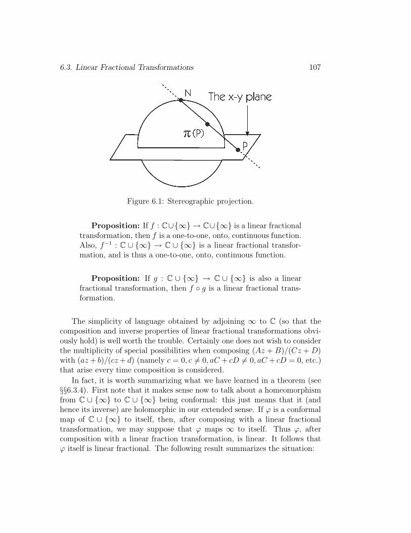
6.3. Linear Fractional Transformations 107
Figure 6.1: Stereographic projection.
Proposition: If f : C∪{∞} → C∪{∞} is a linear fractionaltransformation, then f is a one-to-one, onto, continuous function.Also, f−1 : C ∪ {∞} → C ∪ {∞} is a linear fractional transfor-mation, and is thus a one-to-one, onto, continuous function.
Proposition: If g : C ∪ {∞} → C ∪ {∞} is also a linearfractional transformation, then f ◦ g is a linear fractional trans-formation.
The simplicity of language obtained by adjoining ∞ to C (so that thecomposition and inverse properties of linear fractional transformations obvi-ously hold) is well worth the trouble. Certainly one does not wish to considerthe multiplicity of special possibilities when composing (Az +B)/(Cz + D)with (az+ b)/(cz+ d) (namely c = 0, c 6= 0, aC + cD 6= 0, aC + cD = 0, etc.)that arise every time composition is considered.
In fact, it is worth summarizing what we have learned in a theorem (see§§6.3.4). First note that it makes sense now to talk about a homeomorphismfrom C ∪ {∞} to C ∪ {∞} being conformal: this just means that it (andhence its inverse) are holomorphic in our extended sense. If ϕ is a conformalmap of C ∪ {∞} to itself, then, after composing with a linear fractionaltransformation, we may suppose that ϕ maps ∞ to itself. Thus ϕ, aftercomposition with a linear fraction transformation, is linear. It follows thatϕ itself is linear fractional. The following result summarizes the situation:

108 Chapter 6. Geometric Theory of Holomorphic Functions
6.2.4 Conformal Self-Maps of the Riemann Sphere
Theorem: A function ϕ is a conformal self-mapping of C =C ∪ {∞} to itself if and only if ϕ is linear fractional.
We turn now to the actual utility of linear fractional transformations(beyond their having been the form of automorphisms of D—see §§6.2.1–6.2.3—and the form of all conformal self maps of C ∪ {∞} to itself in thepresent section). One of the most frequently occurring uses is the following:
6.2.5 The Cayley Transform
Theorem (The Cayley Transform): The linear fractional transformationz 7→ (i − z)/(i + z) maps the upper half plane {z : Imz > 0} conformallyonto the unit disc D = {z : |z| < 1}.
6.2.6 Generalized Circles and Lines
Calculations of the type that we have been discussing are straightforwardbut tedious. It is thus worthwhile to seek a simpler way to understand whatthe image under a linear fractional transformation of a given region is. Forregions bounded by line segments and arcs of circles the following result givesa method for addressing this issue:
Let C be the set of subsets of C∪{∞} consisting of (i) circles and (ii) sets ofthe form L∪{∞} where L is a line in C. We call the elements of C “generalizedcircles.” Then every linear fractional transformation ϕ takes elements of Cto elements of C. One verifies this last assertion by noting that any linearfractional transformation is the composition of dilations, translations, andthe inversion map z 7→ 1/z; and each of these component maps clearly sendsgeneralized circles to generalized circles.
6.2.7 The Cayley Transform Revisited
To illustrate the utility of this last result, we return to the Cayley transfor-mation
z 7→ i− z
i+ z. (6.3.7.1)
Under this mapping the point ∞ is sent to −1, the point 1 is sent to(i − 1)/(i + 1) = i, and the point −1 is sent to (i− (−1))/(i+ (−1)) = −i.
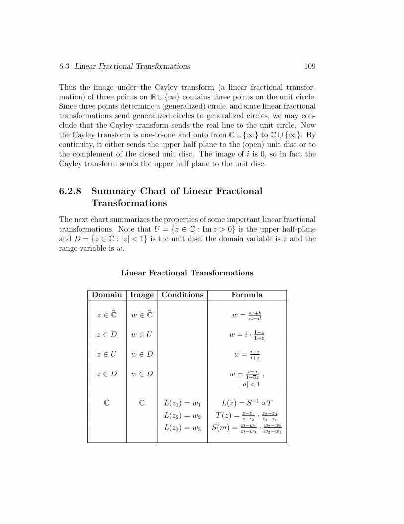
6.3. Linear Fractional Transformations 109
Thus the image under the Cayley transform (a linear fractional transfor-mation) of three points on R∪ {∞} contains three points on the unit circle.Since three points determine a (generalized) circle, and since linear fractionaltransformations send generalized circles to generalized circles, we may con-clude that the Cayley transform sends the real line to the unit circle. Nowthe Cayley transform is one-to-one and onto from C ∪ {∞} to C∪ {∞}. Bycontinuity, it either sends the upper half plane to the (open) unit disc or tothe complement of the closed unit disc. The image of i is 0, so in fact theCayley transform sends the upper half plane to the unit disc.
6.2.8 Summary Chart of Linear Fractional
Transformations
The next chart summarizes the properties of some important linear fractionaltransformations. Note that U = {z ∈ C : Im z > 0} is the upper half-planeand D = {z ∈ C : |z| < 1} is the unit disc; the domain variable is z and therange variable is w.
Linear Fractional Transformations
Domain Image Conditions Formula
z ∈ C w ∈ C w = az+bcz+d
z ∈ D w ∈ U w = i · 1−z1+z
z ∈ U w ∈ D w = i−zi+z
z ∈ D w ∈ D w = z−a1−az ,
|a| < 1
C C L(z1) = w1 L(z) = S−1 ◦ TL(z2) = w2 T (z) = z−z1
z−z3 · z2−z3z2−z1
L(z3) = w3 S(m) = m−w1
m−w3· w2−w3
w2−w1

110 Chapter 6. Geometric Theory of Holomorphic Functions
6.3 The Riemann Mapping Theorem
6.3.1 The Concept of Homeomorphism
Two open sets U and V in C are homeomorphic if there is a one-to-one, onto,continuous function f : U → V with f−1 : V → U also continuous. Such afunction f is called a homeomorphism from U to V (see also §§6.3.3).
6.3.2 The Riemann Mapping Theorem
The Riemann mapping theorem, sometimes called the greatest theorem ofthe nineteenth century, asserts in effect that any planar domain (other thanthe entire plane itself) that has the topology of the unit disc also has theconformal structure of the unit disc. Even though this theorem has beensubsumed by the great uniformization theorem of Kobe (see [FAK]), it isstill striking in its elegance and simplicity:
If U is an open subset of C, U 6= C, and if U is homeomorphicto D, then U is conformally equivalent to D. That is, there is aholomorphic mapping ψ : U → D which is one-to-one and onto.
6.3.3 The Riemann Mapping Theorem: Second
Formulation
An alternative formulation of this theorem uses the concept of “simply con-nected” (see also §§2.3.3.). We say that a connected open set U in thecomplex plane is simply connected if any closed curve in U can be continu-ously deformed to a point. (This is just a precise way of saying that U hasno holes. Yet another formulation of the notion is that the complement of Uhas only one connected component.)
Theorem: If U is an open subset of C, U 6= C, and if U is simplyconnected, then U is conformally equivalent to D.
The proof of the Riemann mapping theorem is long and complex andintroduces many fundamentally new ideas and techniques. We cannot treatit in detail here, but see [GRK]. Certainly the ideas introduced in this proofhave been profoundly influential.Key Steps in the Proof of the Riemann Mapping Theorem:
Fix a point P ∈ U . Assume for simplicity that U is bounded.
6.4. CONFORMAL MAPPINGS OF ANNULI 111
1. Consider
S = {f : f maps D to U, f(0) = P};
2. Define
α = supf∈S
|f(0)| .
3. Use a normal families argument (Montel’s theorem) to show that thereis a function f0 ∈ S so that |f ′
0(0)| = α.
4. Show, using the argument principle, that f0 must be univalent.
5. Show, with a clever proof by contradiction, that if f0 is not onto thenit cannot be the solution of the extremal problem enunciated in 3.
6. The function f0 is the conformal map that we seek.
The full details of the proof of the Riemann mapping theorem appear in[GRK].
6.4 Conformal Mappings of Annuli
6.4.1 A Riemann Mapping Theorem for Annuli
The Riemann mapping theorem tells us that, from the point of view of com-plex analysis, there are only two simply connected planar domains: the discand the plane. Any other simply connected region is biholomorphic to oneof these. It is natural then to ask about domains with holes. Take, for ex-ample, a domain U with precisely one hole. Is it conformally equivalent toan annulus?
Note that if c > 0 is a constant, then for any R1 < R2 the annuli
A1 ≡ {z : R1 < |z| < R2} and A2 ≡ {z : cR1 < |z| < cR2} (6.5.1.1)
are biholomorphically equivalent under the mapping z 7→ cz. The surprisingfact that we shall learn is that these are the only circumstances under whichtwo annuli are equivalent:

112 Chapter 6. Geometric Theory of Holomorphic Functions
6.4.2 Conformal Equivalence of Annuli
LetA1 = {z ∈ C : 1 < |z| < R1} (6.5.2.1)
andA2 = {z ∈ C : 1 < |z| < R2}. (6.5.2.2)
Then A1 is conformally equivalent to A2 if and only if R1 = R2.A perhaps more striking result, and more difficult to prove, is this:
Let U ⊆ C be any bounded domain with one hole—this meansthat the complement of U has two connected components, onebounded and one not. Then U is conformally equivalent to someannulus.
See [AHL] as well as [KRA4] for a discursive discussion of this result.
6.4.3 Classification of Planar Domains
The classification of planar domains up to biholomorphic equivalence is a partof the theory of Riemann surfaces. For now, we comment that one of thestartling classification theorems (a generalization of the Riemann mappingtheorem) is that any bounded planar domain with finitely many “holes” isconformally equivalent to the unit disc with finitely many closed circular arcs,coming from circles centered at the origin, removed. (Here a “hole” in thepresent context means a bounded, connected component of the complementof the domain in C, a concept which coincides with the intuitive idea ofa hole.) An alternative equivalent statement is that any bounded planardomain with finitely many holes is conformally equivalent to the plane withfinitely many vertical slits (see [AHL]). The analogous result for domainswith infinitely many holes is known to be true when the number of holes iscountable (see [HES]).
Chapter 7
Harmonic Functions
7.1 Basic Properties of Harmonic Functions
7.1.1 The Laplace Equation
We reiterate the definition of “harmonic”. Let F be a holomorphic functionon an open set U ⊆ C. Write F = u+ iv, where u and v are real-valued. Thereal part u satisfies a certain partial differential equation known as Laplace’sequation: (
∂2
∂x2+
∂2
∂y2
)u = 0. (7.1.1.1)
(Of course the imaginary part v satisfies the same equation.) In this chapterwe shall study systematically those C2 functions that satisfy this equation.They are called harmonic functions. (Note that we encountered some of theseideas already in §1.4.)
7.1.2 Definition of Harmonic Function
Recall the precise definition of harmonic function:A real-valued function u : U → R on an open set U ⊆ C is harmonic if it
is C2 on U and∆u ≡ 0, (7.1.2.1)
where the Laplacian ∆u is defined by
∆u =
(∂2
∂x2+
∂2
∂y2
)u. (7.1.2.2)
113

114 CHAPTER 7. HARMONIC FUNCTIONS
7.1.3 Real- and Complex-Valued Harmonic Functions
The definition of harmonic function just given applies as well to complex-valued functions. A complex-valued function is harmonic if and only if itsreal and imaginary parts are each harmonic.
The first thing that we need to check is that real-valued harmonic func-tions are just those functions that arise as the real parts of holomorphicfunctions—at least locally.
7.1.4 Harmonic Functions as the Real Parts of
Holomorphic Functions
If u : D(P, r) → R is a harmonic function on a disc D(P, r), then there is aholomorphic function F : D(P, r) → C such that ReF ≡ u on D(P, r). Wealready indicated in Section x.y that this result reduces to solving a coupledsystem of partial differential equations—a situation that can be handled withmulti-variable calculus.
Note that v is uniquely determined by u except for an additive constant:the Cauchy-Riemann equations determine the partial derivatives of v andhence determine v up to an additive constant. One can also think of thedetermination, up to a constant, of v by u in another way: If v is anotherfunction such that u+iv is holomorphic, thenH ≡ i(v−v) = (u+iv)−(u+iv)is a holomorphic function with zero real part; hence its image is not open.ThusH must be a constant, and v and v differ by a constant. Any (harmonic)function v such that u+ iv is holomorphic is called a harmonic conjugate ofu (again see §§1.4.2).
Theorem: If U is a simply connected open set (see §§6.4.3) andif u : U → R is a harmonic function, then there is a C2 (indeed aC∞) harmonic function v such that u+iv : U → C is holomorphic.
Another important relationship between harmonic and holomorphic func-tions is this:
If u : U → R is harmonic and if H : V → U is holomorphic, thenu ◦H is harmonic on V .
This result is proved by direct calculation (i.e., differentiation, using the chainrule).

7.2. The Maximum Principle 115
7.1.5 Smoothness of Harmonic Functions
If u : U → R is a harmonic function on an open set U ⊆ C, then u ∈C∞. In fact a harmonic function is always real analytic (has a local powerseries expansion in powers of x and y). This follows, for instance, becausea harmonic function is locally the real part of a holomorphic function (see§§1.4.2, §§7.1.4). A holomorphic function has a power series expansion abouteach point, so is certainly infinitely differentiable.
7.2 The Maximum Principle and the Mean
Value
Property
7.2.1 The Maximum Principle for Harmonic Functions
Theorem: If u : U → R is harmonic on a connected openset U and if there is a point P0 ∈ U with the property thatu(P0) = maxz∈U u(z), then u is constant on U . Compare themaximum modulus principle for holomorphic functions in §§5.4.1.The proof, using (7.2.4.1) below, is essentially the same as thatfor the maximum principle for holomorphic functions.
7.2.2 The Minimum Principle for Harmonic Functions
Theorem: If u : U → R is a harmonic function on a connectedopen set U ⊆ C and if there is a point P0 ∈ U such that u(P0) =minQ∈U u(Q), then u is constant on U . Compare the minimumprinciple for holomorphic functions in §§5.4.3.
The reader may note that the minimum principle for holomorphic func-tions requires an extra hypothesis (i.e., non-vanishing of the function) whilethat for harmonic functions does not. The difference may be explained bynoting that with harmonic functions we are considering the real-valued func-tion u, while with holomorphic functions we must restrict attention to themodulus function |f |.

116 Chapter 7. Harmonic Functions
7.2.3 The Boundary Maximum and Minimum Princi-
ples
An important and intuitively appealing consequence of the maximum princi-ple is the following result (which is sometimes called the “boundary maximumprinciple”). Recall that a continuous function on a compact set assumes amaximum value. When the function is harmonic, the maximum occurs atthe boundary in the following precise sense:
Theorem: Let U ⊆ C be a bounded domain. Let u be a contin-uous, real-valued function on the closure U of U that is harmonicon U . Then
maxU
u = max∂U
u. (7.2.3.1)
The analogous result for the minimum is:
Theorem: Let U ⊆ C be a domain and let u be a continuousfunction on the closure U of U that is harmonic on U . Then
minUu = min
∂Uu. (7.2.3.2)
Compare the analogous results for holomorphic functions in §§5.4.2, 5.4.3.
7.2.4 The Mean Value Property
Suppose that u : U → R is a harmonic function on an open set U ⊆ C andthat D(P, r) ⊆ U for some r > 0. Then
u(P ) =1
2π
∫ 2π
0
u(P + reiθ) dθ. (7.2.4.1)
We will see in §§7.4.1 that the mean value property characterizes harmonicfunctions.
The mean value property for harmonic functions can be proved on theunit disc by first verifying it for the monomials zj and zj and then notingthat any harmonic function is in the closed linear span of these. It canalso be checked because a harmonic function is (locally) the real part of a
7.3. THE POISSON INTEGRAL FORMULA 117
holomorphic function and so the result can be derived (by taking the realpart) from that for a holomorphic function. A very interesting proof mayalso be gotten from Green’s theorem (see [KRA5]).
We conclude this subsection with two alternative formulations of the meanvalue property (MVP). Either one may be derived with simple changes ofvariable in the integral. In both cases, u, U, P, r are as above.
First Alternative Formulation of MVP
u(P ) =1
πr2
∫∫
D(P,r)
u(x, y) dxdy.
Second Alternative Formulation of MVP
u(P ) =1
2πr
∫
∂D(P,r)
u(ζ) dσ(ζ),
where dσ is arc-length measure on ∂D(P, r).
7.2.5 Boundary Uniqueness for Harmonic Functions
If u1 : D(0, 1) → R and u2 : D(0, 1) → R are two continuous functions, eachof which is harmonic on D(0, 1) and if u1 = u2 on ∂D(0, 1) = {z : |z| = 1},then u1 ≡ u2. This assertion follows from the boundary maximum principle(§§7.2.3.1) applied to u1 − u2. Thus, in effect, a harmonic function u onD(0, 1) that extends continuously to D(0, 1) is completely determined by itsvalues on D(0, 1) \D(0, 1) = ∂D(0, 1). Of course an analogous result holdson any domain in C.
7.3 The Poisson Integral Formula
7.3.1 The Poisson Integral
The next result builds on the boundary uniqueness idea. After all, if aharmonic function on the interior of a disc is completely determined by itsboundary values, then we ought to be able to calculate the interior valuesfrom the boundary values. This is in fact what the Poisson integral formuladoes for us.

118 Chapter 7. Harmonic Functions
Let u : U → R be a harmonic function on a neighborhood of D(0, 1).Then, for any point a ∈ D(0, 1),
u(a) =1
2π
∫ 2π
0
u(eiψ) · 1 − |a|2|a− eiψ|2 dψ. (7.3.1.1)
7.3.2 The Poisson Kernel
The expression1
2π
1 − |a|2|a− eiψ|2 (7.3.2.1)
is called the Poisson kernel for the unit disc. It is often convenient to rewritethe formula we have just enunciated by setting a = |a|eiθ = reiθ. Then theresult says that
u(reiθ) =1
2π
∫ 2π
0
u(eiψ)1 − r2
1 − 2r cos(θ − ψ) + r2dψ. (7.3.2.2)
In other words
u(reiθ) =
∫ 2π
0
u(eiθ)Pr(θ − ψ) dψ, (7.3.2.3)
where
Pr(θ − ψ) =1
2π
1 − r2
1 − 2r cos(θ − ψ) + r2. (7.3.2.4)
There are a number of ways to verify the Poisson integral formula. First,one could use Green’s theorem (for which see again [KRA5]). Alternatively,one could first verify the formula with barehand calculation in the case thatf(z) = zk or f(z) = zk. A third possibility is to note that formula (7.3.2.2)is plainly true at the origin (i.e., when r = 0). Then spread the result tothe rest of the disc using conformal self-maps of the disc and the conformalinvariance of harmonic functions. We leave the details to the reader.
7.3.3 The Dirichlet Problem
The Poisson integral formula both reproduces and creates harmonic func-tions. But, in contrast to the holomorphic case (§2.4), there is a simpleconnection between a continuous function f on ∂D(0, 1) and the createdharmonic function u on D. The following theorem states this connectionprecisely. The theorem is usually called “the solution of the Dirichlet prob-lem on the disc”:

7.3. THE POISSON INTEGRAL FORMULA 119
7.3.4 The Solution of the Dirichlet Problem on the
Disc
Theorem: Let f be a continuous function on ∂D(0, 1). Define
u(z) =
1
2π
∫ 2π
0
f(eiψ) · 1 − |z|2|z − eiψ|2 dψ if z ∈ D(0, 1)
f(z) if z ∈ ∂D(0, 1).(7.3.4.1)
Then u is continuous on D(0, 1) and harmonic on D(0, 1). Theproof of this theorem is rather technical, and we refer the readerto [GRK] or [KRA5].
Closely related to this result is the reproducing property of the Poissonkernel:
Theorem: Let u be harmonic on a neighborhood of D(0, 1).Then, for z ∈ D(0, 1),
u(z) =1
2π
∫ 2π
0
u(eiψ) · 1 − |z|2|z − eiψ|2 dψ . (7.3.4.2)
See (7.3.1.1). One way to understand this last formula is to ver-ify by hand that the Poisson kernel is harmonic in the variablez. Then (7.3.4.2) creates a function that agrees with u on theboundary of the disc and is harmonic inside, so it must be uitself.
7.3.5 The Dirichlet Problem on a General Disc
A change of variables shows that the results of §§7.3.4 remain true on ageneral disc. To wit, let f be a continuous function on ∂D(P, r). Define
u(z) =
1
2π
∫ 2π
0
f(eiψ) · R − |z − P |2|(z − P ) −Reiψ|2 dψ if z ∈ D(P,R)
f(z) if z ∈ ∂D(P,R).(7.3.5.1)
Then u is continuous on D(P,R) and harmonic on D(P,R).
120 Chapter 7. Harmonic Functions
If instead u is harmonic on a neighborhood of D(P,R), then, for z ∈D(P,R),
u(z) =1
2π
∫ 2π
0
u(P +Reiψ) · R2 − |z − P |2|(z − P ) − Reiψ|2 dψ. (7.3.5.2)
7.4 Regularity of Harmonic Functions
7.4.1 The Mean Value Property on Circles
A continuous function h : U → R on an open set U ⊆ C has the εP -mean value property if, for each point P ∈ U, there is an εP > 0 such thatD(P, εP ) ⊆ U and, for every 0 < ε < εP ,
h(P ) =1
2π
∫ 2π
0
h(P + εeiθ)dθ. (7.4.1.1)
The εP -mean value property allows the size of εP to vary arbitrarily withP .
Theorem: If h : U → R is a continuous function on an open setU with the εP -mean value property, then h is harmonic.
Again, the proof of this result is too technical to treat here. See [GRK].
7.4.2 The Limit of a Sequence of Harmonic Functions
If {hj} is a sequence of real-valued harmonic functions that converges uni-formly on compact subsets of U to a function h : U → R, then h is harmonicon U . This is immediate from the Poisson integral formula, since we nowknow that the Poisson kernel is harmonic.
7.5 The Schwarz Reflection Principle
7.5.1 Reflection of Harmonic Functions
We present in this section an application of what we have learned so far toa question of extension of a harmonic function to a larger domain. This willalready illustrate the importance and power of harmonic function theory andwill provide us with a striking result about holomorphic functions as well.

7.5. THE SCHWARZ REFLECTION PRINCIPLE 121
7.5.2 Schwarz Reflection Principle for Harmonic Func-
tions
Let V be a connected open set in C. Suppose that
V ∩ (real axis) = {x ∈ R : a < x < b}.
Set U = {z ∈ V : Im z > 0}. Assume that v : U → R is harmonicand that, for each ζ ∈ V ∩ (real axis),
limU3z→ζ
v(z) = 0. (7.5.2.1)
Set U = {z : z ∈ U}. Define
v(z) =
v(z) if z ∈ U0 if z ∈ V ∩ (real axis)
−v(z) if z ∈ U .
(7.5.2.2)
Then v is harmonic on U∗ ≡ U ∪ U ∪ {x ∈ R : a < x < b}.
This result provides a way of extending a harmonic function from a givenopen set to a larger (reflected) open set. The method is known as the Schwarz
Reflection Principle. One can think of U as the reflection of U in the realaxis, and the definition of v on U as the correspondingly appropriate idea ofreflecting the function v. See Figure 7.1.
The proof of Schwarz reflection is a clever argument involving the sym-metries of the Poisson integral formula. We refer the reader to [GRK] for thedetails.
7.5.3 The Schwarz Reflection Principle for Holomor-
phic Functions
Theorem: Let V be a connected open set in C such that V ∩(the real axis) = {x ∈ R : a < x < b} for some a, b ∈ R. SetU = {z ∈ V : Im z > 0}. Suppose that F : U → C is holomorphicand that

122 Chapter 7. Harmonic Functions
Figure 7.1: Schwarz reflection.
limU3z→x
ImF (z) = 0 (7.5.3.1)
for each ζ ∈ V ∩ (real axis). Define U = {z ∈ C : z ∈ U}. Then
there is a holomorphic function G on U ∪ U ∪{x ∈ R : a < x < b}such that G
∣∣U
= F . In fact ϕ(ζ) ≡ limU3z→ζ ReF (z) exists foreach ζ ∈ V ∩ (real axis) and
G(z) =
F (z) if z ∈ Uϕ(z) + i0 if z ∈ V ∩ (real axis)
F (z) if z ∈ U .
(7.5.3.2)
7.5.4 More General Versions of the Schwarz Reflection
Principle
We take this opportunity to note that Schwarz reflection is not simply afact about reflection in lines. Since lines are conformally equivalent (by wayof linear fractional transformations) to circles, it is also possible to performSchwarz reflection in a circle (with suitably modified hypotheses). More istrue: in fact one can conformally map a neighborhood of any real analytic

7.6. HARNACK’S PRINCIPLE 123
curve to a line segment; so, with some extra effort, Schwarz reflection maybe performed in any real analytic arc.
7.6 Harnack’s Principle
7.6.1 The Harnack Inequality
Theorem: Let u be a non-negative, harmonic function onD(0, R).Then, for any z ∈ D(0, R),
R− |z|R + |z| · u(0) ≤ u(z) ≤ R + |z|
R − |z| · u(0). (7.6.1.1)
More generally:
Let u be a non-negative, harmonic function on D(P,R). Then,for any z ∈ D(P,R),
R− |z − P |R + |z − P | · u(P ) ≤ u(z) ≤ R + |z − P |
R− |z − P | · u(P ). (7.6.1.2)
In fact these extremely useful estimates are a direct reflection of the sizeof the Poisson kernel. The reader may provide the details.
7.6.2 Harnack’s Principle
Theorem: Let u1 ≤ u2 ≤ . . . be harmonic functions on a con-nected open set U ⊆ C. Then either uj → ∞ uniformly oncompact sets or there is a (finite-valued) harmonic function u onU such that uj → u uniformly on compact sets.
The reader may prove this assertion as a simple application of the Harnackinequalities and a little logic.

124 Chapter 7. Harmonic Functions
7.7 The Dirichlet Problem and Subharmonic
Functions
7.7.1 The Dirichlet Problem
Let U ⊆ C be an open set, U 6= C. Let f be a given continuous functionon ∂U . Does there exist a continuous function u on U such that u
∣∣∂U
= fand u is harmonic on U? If u exists, is it unique? These two questionstaken together are called the Dirichlet problem for the domain U . [Note thatwe have already solved the Dirichlet problem when U is the unit disc—see§§7.3.1, §§7.3.4.] It has many motivations from physics (see [COH], [LOG]).For instance, suppose that a flat, thin film of heat-conducting material isin thermal equilibrium. That is, the temperature at each point of the filmis constant with passing time (§§14.2.2). Then its temperature at variouspoints is a harmonic function (see [KRA1]). Physical intuition suggests thatif the boundary ∂U of the film has a given temperature distribution f :∂U → R, then the temperatures at interior points are uniquely determined.Historically, physicists have found this intuition strongly compelling.
From the viewpoint of mathematical proof, as opposed to physical intu-ition, the situation is more complicated. The result of §§7.3.4 asserts in effectthat the Dirichlet problem on the unit disc always has a solution. And, onany bounded domain U , it has only one solution corresponding to any givenboundary function f , because of the (boundary) maximum principle: If u1
and u2 are both solutions, then u ≡ u1 − u2 is harmonic and is zero onthe boundary, so that u1 − u2 ≡ 0, hence u1 ≡ u2. While this reasoningdemonstrates that the Dirichlet problem on a bounded open set U can haveat most one solution, it is also the case that on more complicated domainsthe Dirichlet problem may not have any solution.
7.7.2 Conditions for Solving the Dirichlet Problem
The Dirichlet problem is not always solvable on the domain U = D(0, 1)\{0};in fact the data f(z) = 1 when |z| = 1 and f(z) = 0 when z = 0 have nosolution—see [GK, p. 229]. Thus some conditions on ∂U are necessary inorder that the Dirichlet problem be solvable for U . It will turn out that if∂U consists of “smooth” curves, then the Dirichlet problem is always solvable.The best possible general result is that if each connected component of theboundary of U contains more than one point, then the Dirichlet problem
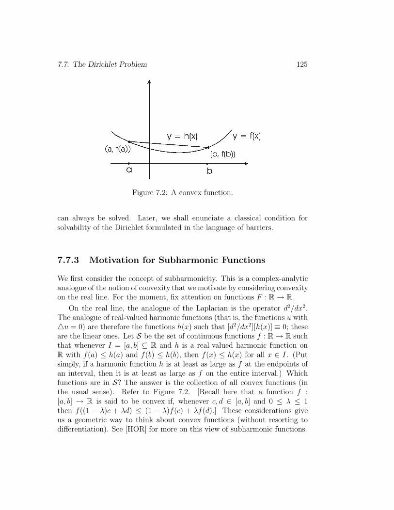
7.7. The Dirichlet Problem 125
Figure 7.2: A convex function.
can always be solved. Later, we shall enunciate a classical condition forsolvability of the Dirichlet formulated in the language of barriers.
7.7.3 Motivation for Subharmonic Functions
We first consider the concept of subharmonicity. This is a complex-analyticanalogue of the notion of convexity that we motivate by considering convexityon the real line. For the moment, fix attention on functions F : R → R.
On the real line, the analogue of the Laplacian is the operator d2/dx2.The analogue of real-valued harmonic functions (that is, the functions u with4u = 0) are therefore the functions h(x) such that [d2/dx2][h(x)] ≡ 0; theseare the linear ones. Let S be the set of continuous functions f : R → R suchthat whenever I = [a, b] ⊆ R and h is a real-valued harmonic function onR with f(a) ≤ h(a) and f(b) ≤ h(b), then f(x) ≤ h(x) for all x ∈ I . (Putsimply, if a harmonic function h is at least as large as f at the endpoints ofan interval, then it is at least as large as f on the entire interval.) Whichfunctions are in S? The answer is the collection of all convex functions (inthe usual sense). Refer to Figure 7.2. [Recall here that a function f :[a, b] → R is said to be convex if, whenever c, d ∈ [a, b] and 0 ≤ λ ≤ 1then f((1 − λ)c + λd) ≤ (1 − λ)f(c) + λf(d).] These considerations giveus a geometric way to think about convex functions (without resorting todifferentiation). See [HOR] for more on this view of subharmonic functions.

126 Chapter 7. Harmonic Functions
7.7.4 Definition of Subharmonic Function
Our definition of subharmonic function on a domain in C (or R2) is motivatedby the discussion of convexity in the preceding subsection.
Definition: Let U ⊆ C be an open set and f a real-valued,continuous function on U . Suppose that for eachD(P, r) ⊆ U andevery real-valued harmonic function h defined on a neighborhoodof D(P, r) which satisfies f ≤ h on ∂D(P, r), it holds that f ≤ hon D(P, r). Then f is said to be subharmonic on U .
7.7.5 Other Characterizations of Subharmonic
Functions
A function f : U → R that is C2 is subharmonic if and only if 4f ≥ 0 every-where. This is analogous to the fact that a C2 function on (an open set in) R
is convex if and only if it has non-negative second derivative everywhere—andthe proof is quite similar. The next result will allow us to identify many sub-harmonic functions which are only continuous, not C2, so that the 4f ≥ 0criterion is not applicable.
Let f : U → R be continuous. Suppose that, for each D(P, r) ⊆ U ,
f(P ) ≤ 1
2π
∫ 2π
0
f(P + reiθ)dθ (7.7.5.1)
(this is called the sub-mean value property). Then f is subharmonic. Thisresult is derived directly from the mean value property for harmonic func-tions.
Conversely, if f : U → R is a continuous, subharmonic function and ifD(P, r) ⊆ U , then the inequality (7.7.5.1) holds.
7.7.6 The Maximum Principle
A consequence of the sub-mean value property (7.7.5.1) is the maximumprinciple for subharmonic functions:
If f is subharmonic on U and if there is a P ∈ U such thatf(P ) ≥ f(z) for all z ∈ U , then f is constant.

7.7. The Dirichlet Problem 127
It may be noted that if f is holomorphic then |f | is subharmonic; this explainswhy a holomorphic function satisfies the maximum principle. The proof ofthis new maximum principle is identical to proofs of this principle that wehave seen in other contexts—see, for example, §§7.2.1, 7.2.2, 7.2.3.
7.7.7 Lack of A Minimum Principle
We note in passing that there is no “minimum principle” for subharmonicfunctions. Subharmonicity is a “one-sided” property. Put in other words,the negative of a subharmonic function is not subharmonic.
7.7.8 Basic Properties of Subharmonic Functions
Here are some properties of subharmonic functions that are worth noting.The third of these explains why subharmonic functions are a much moreflexible tool than holomorphic or even harmonic functions. The proofs areimmediate from the definitions and the properties of harmonic funcitons dis-cussed thus far.
1. If f1, f2 are subharmonic functions on U , then so is f1 + f2.
2. If f1 is subharmonic on U and α > 0 is a constant, then αf1 is subhar-monic on U .
3. If f1, f2 are subharmonic on U then g(z) ≡ max{f1(z), f2(z)} is alsosubharmonic on U .
7.7.9 The Concept of a Barrier
The next notion that we need to introduce is that of a barrier. Namely, wewant to put a geometric-analytic condition on the boundary of a domainthat will rule out examples like the punctured disc in §§7.7.2 (in which theDirichlet problem could not be solved). The definition of a barrier at a pointP ∈ ∂U is a bit technical, but the existence of a barrier will turn out tobe exactly the hypothesis needed for the construction of the solution of theDirichlet problem.
Definition: Let U ⊆ C be an open set and P ∈ ∂U . We call afunction b : U → R a barrier for U at P if
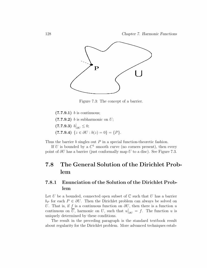
128 Chapter 7. Harmonic Functions
P
Figure 7.3: The concept of a barrier.
(7.7.9.1) b is continuous;
(7.7.9.2) b is subharmonic on U ;
(7.7.9.3) b∣∣∂U
≤ 0;
(7.7.9.4) {z ∈ ∂U : b(z) = 0} = {P}.
Thus the barrier b singles out P in a special function-theoretic fashion.If U is bounded by a C1 smooth curve (no corners present), then every
point of ∂U has a barrier (just conformally map U to a disc). See Figure 7.3.
7.8 The General Solution of the Dirichlet Prob-
lem
7.8.1 Enunciation of the Solution of the Dirichlet Prob-
lem
Let U be a bounded, connected open subset of C such that U has a barrierbP for each P ∈ ∂U . Then the Dirichlet problem can always be solved onU . That is, if f is a continuous function on ∂U , then there is a function ucontinuous on U , harmonic on U , such that u
∣∣∂U
= f . The function u isuniquely determined by these conditions.
The result in the preceding paragraph is the standard textbook resultabout regularity for the Dirichlet problem. More advanced techniques estab-

7.8. The General Solution 129
lish that if each connected component of ∂U has at least two points then theDirichlet problem is solvable on U .
The solution of the Dirichlet problem in the generality that we have beendiscussing here is a technical tour de force. See [GRK] for all the details.The basic idea is that (i) there exists some subharmonic function whoseboundary limits lie below the given boundary data function f ; (ii) we definea new function u to be the pointwise supremum of all such subharmonicfunctions; and (iii) then the Harnack principle and the maximum principle(along with the barriers) can be used to show that the function u constructedin (ii) is harmonic and agrees with f at each boundary point.

130 Chapter 7. Harmonic Functions

Chapter 8
Infinite Series and Products
8.1 Basic Concepts Concerning Infinite Sums
and Products
8.1.1 Uniform Convergence of a Sequence
Let U ⊆ C be an open set and gj : U → C functions. Recall (§3.1.5) thatthe sequence {gj} is said to converge uniformly on compact subsets of Uto a function g if the following condition holds: For each compact K ⊆ U(see §§3.1.5) and each ε > 0 there is an N > 0 such that if j > N , then|g(z) − gj(z)| < ε for all z ∈ K. It should be noted that, in general, thechoice of N depends on ε and on K, but not on the particular point z ∈ K.
8.1.2 The Cauchy Condition for a Sequence of Func-
tions
Because of the completeness (see [RUD1], [KRA2]) of the complex numbers,a sequence of functions is uniformly convergent on compact sets if and onlyif it is (what is called) uniformly Cauchy on compact sets. Here a sequenceof functions is said to be uniformly Cauchy on compact sets if, for each Kcompact in U and each ε > 0, there is an N > 0 such that: for all j, k > N andall z ∈ K we have |gj(z)−gk(z)| < ε. The Cauchy condition is useful becauseit does not make explicit reference to the limit function g. One can therebyverify uniform convergence to some limit without previously determining thelimit function explicitly.
131

132 CHAPTER 8. INFINITE SERIES AND PRODUCTS
8.1.3 Normal Convergence of a Sequence
For the purposes of complex analysis, the basic fact about uniform conver-gence on compact sets is our result which states that if {gj} are holomorphicfunctions on U and if the gj converge uniformly on compact subsets of U toa function g, then g is holomorphic (§§3.1.5). In these circumstances we willsay that {gj} converges normally to g.
8.1.4 Normal Convergence of a Series
If f1, f2, . . . are functions on U , then we may study the convergence propertiesof ∞∑
j=1
fj. (8.1.4.1)
The series converges normally if its sequence of partial sums
SN(z) =
N∑
j=1
fj(z) , N = 1, 2, . . . (8.1.4.2)
converges normally in U . The function
f(z) =
∞∑
j=1
fj(z) (8.1.4.3)
will then be holomorphic because it is the normal limit of the partial sumsSN (each of which is holomorphic).
8.1.5 The Cauchy Condition for a Series
There is a Cauchy condition for normal convergence of a series: the series
∞∑
j=1
fj(z) (8.1.5.1)
is said to be uniformly Cauchy on compact sets if, for each compact K ⊆ Uand each ε > 0, there is an N > 0 such that for all M ≥ L > N it holds that
∣∣∣∣∣
M∑
j=L
fj(z)
∣∣∣∣∣ < ε. (8.1.5.2)

8.1. BASIC CONCEPTS 133
[Note that this is just a reformulation of the Cauchy condition for the se-quence of partial sums SN (z).] It is easy to see that a series that is uniformlyCauchy converges normally to its limit function.
8.1.6 The Concept of an Infinite Product
Now we turn to products. One of the principal activities in complex analysisis to construct holomorphic or meromorphic functions with certain prescribedbehavior. For some problems of this type, it frequently turns out that infiniteproducts are more useful than infinite sums. The reason is that, for instance,if we want to construct a function that will vanish on a certain infinite set{aj}, then we could hope to find individual functions fj that vanish at aj andthen multiply the fj’s together. This process requires that we make sense ofthe notion of “infinite product.”
8.1.7 Infinite Products of Scalars
We begin with infinite products of complex numbers, and then adapt theideas to infinite products of functions. For reasons that will become apparentmomentarily, it is convenient to write products in the form
∞∏
j=1
(1 + aj), (8.1.7.1)
where aj ∈ C. The symbol∏
stands for multiplication. We want to definewhat it means for a product such as (8.1.7.1) to converge.
8.1.8 Partial Products
First define the partial products PN of (8.1.7.1) to be
PN =
N∏
j=1
(1 + aj) ≡ (1 + a1) · (1 + a2) · · · (1 + aN ). (8.1.8.1)
We might be tempted to say that the infinite product
∞∏
j=1
(1 + aj) (8.1.8.2)

134 CHAPTER 8. INFINITE SERIES AND PRODUCTS
converges if the sequence of partial products {PN} converges. But, for tech-nical reasons, a different definition is more useful.
8.1.9 Convergence of an Infinite Product
An infinite product∞∏
j=1
(1 + aj) (8.1.9.1)
is said to converge if
(8.1.8.2) Only a finite number aj1 , . . . , ajk of the aj’s are equal to −1.
(8.1.9.3) If N0 > 0 is so large that aj 6= −1 for j > N0, then
limN→+∞
N∏
j=N0+1
(1 + aj) (8.1.9.3.1)
exists and is non-zero.
8.1.10 The Value of an Infinite Product
If∏∞
j=1(1 + aj) converges, then we define its value to be (with N0 as in(8.1.9.3)) [
N0∏
j=1
(1 + aj)
]· limN→+∞
N∏
N0+1
(1 + aj). (8.1.10.1)
8.1.11 Products That Are Disallowed
As the exposition develops, it will become clear why we wish to disallowproducts with
limN→+∞
N∏
j=N0+1
(1 + aj) = 0. (8.1.11.1)

8.1. BASIC CONCEPTS 135
8.1.12 Condition for Convergence of an Infinite Prod-
uct
If ∞∑
j=1
|aj| <∞ , (8.1.12.1)
then ∞∏
j=1
(1 + |aj|) (8.1.12.2)
converges. [See (8.1.12.6), (8.1.12.7) for part of the mathematical reason asto why these assertions are true.] The facts all hinge on the basic identityeα = 1 + α+ · · · .
If ∞∏
j=1
(1 + |aj|) (8.1.12.3)
converges, then∞∑
j=1
|aj| (8.1.12.4)
converges.Let aj ∈ C. Set
PN =N∏
j=1
(1 + aj) , PN =N∏
j=1
(1 + |aj|). (8.1.12.5)
Then
(8.1.12.6) PN ≤ exp (|a1| + · · · + |aN |).
(8.1.12.7) |PN − 1| ≤ PN − 1.
If the infinite product∞∏
j=1
(1 + |aj|) (8.1.12.8)
converges, then so does∞∏
j=1
(1 + aj). (8.1.12.9)

136 CHAPTER 8. INFINITE SERIES AND PRODUCTS
If∞∑
j=1
|aj| <∞ , (8.1.12.10)
then∞∏
j=1
(1 + aj) (8.1.12.11)
converges.
This last is our most useful convergence result for infinite products. It isso important that it is worth restating in a standard alternative form: If
∞∑
j=1
|1 − aj| <∞ , (8.1.12.12)
then∞∏
j=1
aj (8.1.12.13)
converges. The proof is just a change of notation.
8.1.13 Infinite Products of Holomorphic Functions
We now apply these considerations to infinite products of holomorphic func-tions.
Let U ⊆ C be open. Suppose that fj : U → C are holomorphic and that
∞∑
j=1
|fj| (8.1.13.1)
converges uniformly on compact subsets of U . Then the sequence of partialproducts
FN (z) =
N∏
j=1
(1 + fj(z)) (8.1.13.2)
converges uniformly on compact subsets of U . In particular, the limit ofthese partial products defines a holomorphic function on U .

8.2. Weierstrass Factorization 137
8.1.14 Vanishing of an Infinite Product
The function f defined on a domain U by the product
f(z) =∞∏
j=1
(1 + fj(z)) (8.1.14.1)
vanishes at a point z0 ∈ U if and only if fj(z0) = −1 for some j. Themultiplicity of the zero at z0 is the sum of the multiplicities of the zeros ofthe functions 1 + fj at z0.
8.1.15 Uniform Convergence of an Infinite Product
of Functions
Remark: For convenience, one says that the product∏∞
1 (1 + fj(z)) con-verges uniformly on a set E if
(8.1.15.1) it converges for each z in E
and
(8.1.15.2) the sequence {∏N1 (1+fj(z))} converges uniformly onE to
∏∞1 (1+
fj(z)).
Then our main convergence result can be summarized as follows:
8.1.16 Condition for the Uniform Convergence of an
Infinite Product of Functions
Theorem: If∑∞
j=1 |fj | converges uniformly on compact sets,then the product
∏∞1 (1+ fj(z)) converges uniformly on compact
sets.
It should be noted that the convergence conditions in §§8.1.9 are satisfiedautomatically in the situation of this last theorem.
138 CHAPTER 8. INFINITE SERIES AND PRODUCTS
8.2 The Weierstrass Factorization Theorem
8.2.1 Prologue
One of the most significant facts about a polynomial function p(z) of z ∈ C
is that it can be factored (see §§3.1.4):
p(z) = c ·k∏
j=1
(z − aj). (8.2.1.1)
Among other things, such a factorization facilitates the study of the zerosof p. In this section we shall show that in fact any entire function can befactored in such a way that each multiplicative factor possesses precisely onezero (of first order). Since a function holomorphic on all of C (called anentire function) can have infinitely many zeros, the factorization must be aninfinite product in at least some cases. We consider such a factorization inthis section.
8.2.2 Weierstrass Factors
To obtain the Weierstrass factors, we define
E0(z) = 1 − z (8.2.2.1)
and for 1 ≤ p ∈ Z we let
Ep(z) = (1 − z) exp
(z +
z2
2+ · · · + zp
p
). (8.2.2.2)
Of course each Ep is holomorphic on all of C. The factorization theory hingeson a technical calculation that says that, in some sense, Ep is close to 1 if |z|is small. This assertion is not surprising since
(z +
z2
2+ · · · + zp
p
)(8.2.2.3)
is the initial part of the power series of − log(1 − z). Thus
(1 − z) exp
(z +
z2
2+ · · · + zp
p
)(8.2.2.4)
might be expected to be close to 1 for z small (and p large).

8.3. Weierstrass and Mittag-Leffler Theorems 139
8.2.3 Convergence of the Weierstrass Product
Theorem: Let {an}∞n=1 be a sequence of non-zero complex num-bers with no accumulation point in the complex plane (note, how-ever, that the ans need not be distinct). If {pn} are positiveintegers that satisfy
∞∑
n=1
(r
|an|
)pn+1
<∞ (8.2.3.1)
for every r > 0, then the infinite product
∞∏
n=1
Epn
(z
an
)(8.2.3.2)
(called a Weierstrass product) converges uniformly on compactsubsets of C to an entire function F . The zeros of F are preciselythe points {an}, counted with multiplicity.
8.2.4 Existence of an Entire Function with PrescribedZeros
Let {an}∞n=1 be any sequence in the plane with no finite accumulation point.Then there exists an entire function f with zero set precisely equal to {an}∞n=1
(counting multiplicities). The function f is given by a Weierstrass product.
8.2.5 The Weierstrass Factorization Theorem
Theorem: Let f be an entire function. Suppose that f vanishesto order m at 0, m ≥ 0. Let {an} be the other zeros of f, listedwith multiplicities. Then there is an entire function g such that
f(z) = zm · eg(z)∞∏
n=1
En−1
(z
an
). (8.2.5.1)

140 CHAPTER 8. INFINITE SERIES AND PRODUCTS
8.3 The Theorems of Weierstrass and
Mittag-Leffler
8.3.1 The Concept of Weierstrass’s Theorem
Let U ⊂ C be a domain. The only necessary condition that we know for aset {aj} ⊆ U to be the zero set of a function f holomorphic on U is that{aj} have no accumulation point in U . It is remarkable that this conditionis also sufficient: that is the content of Weierstrass’s theorem.
8.3.2 Weierstrass’s Theorem
Theorem: Let U ⊆ C be any open set. Let a1, a2, . . . be afinite or infinite sequence in U (possibly with repetitions) thathas no accumulation point in U . Then there exists a holomorphicfunction f on U whose zero set is precisely {aj}. (The functionf is constructed by taking an infinite product.)
The proof converts the problem to a situation on the entire plane, and thenuses the Weierstrass product.
We next want to formulate a result about maximal domains of existence(or domains of definition) of holomorphic functions. But first we need ageometric fact about open subsets of the plane.
8.3.3 Construction of a Discrete Set
Let U ⊂6=
C be any open set. Then there exists a countably infinite set A ⊆ U
such that
(8.3.3.1) A has no accumulation point in U .
(8.3.3.2) Every P ∈ ∂U is an accumulation point of A.
See Figure 8.1. Details of this construction appear in [GRK, p. 268].
8.3.4 Domains of Existence for Holomorphic Functions

8.3. Weierstrass and Mittag-Leffler Theorems 141
Figure 8.1: Any domain in C is a domain of holomorphy.
Theorem: Let U ⊆ C be any proper, connected, open subset.There is a function f holomorphic on U such that f cannot beanalytically continued past any P ∈ ∂U (see also §§9.2.2 on theconcept of “regular boundary point”).
The verification of this last result is just to apply Weierstrass’s theorem tothe discrete set described in §§8.3.3. This yields a non-constant holomorphicfunction f on U whose zero set accumulates at every boundary point of U .If f were to analytically continue to any strictly larger open set U , thenU would contain a point of ∂U , hence would have an interior accumulationpoint of the zeros of f . Thus f would be identically zero, and that would bea contradiction.
8.3.5 The Field Generated by the Ring of Holomorphic
Functions
Another important corollary of Weierstrass’s theorem is that, for any openU, the field generated by the ring of holomorphic functions on U is the fieldof all meromorphic functions on U . In simpler language:
Let U ⊆ C be open. Let m be meromorphic on U . Then thereare holomorphic functions f, g on U such that

142 CHAPTER 8. INFINITE SERIES AND PRODUCTS
m(z) =f(z)
g(z). (8.3.5.1)
8.3.6 The Mittag-Leffler Theorem
Since it is possible to prescribe zeros of a holomorphic function on any openU, then of course we can (in principle) prescribe poles—since 1/f has polesexactly where f has zeros. But we can do better: with a little extra workwe can prescribe the negative power portion of the Laurent series on anydiscrete subset of U .
We now formulate the basic result on prescribing pole behavior, knownas the Mittag-Leffler theorem, in two different (but equivalent) ways: onequalitative and the other quantitative.
Mittag-Leffler Theorem: First Version
Let U ⊆ C be any open set. Let α1, α2, . . . be a finite or countablyinfinite set of distinct elements of U with no accumulation point inU . Suppose, for each j, that Uj is a neighborhood of αj. Furtherassume, for each j, that mj is a meromorphic function definedon Uj with a pole at αj and no other poles. Then there exists ameromorphic m on U such that m−mj is holomorphic on Uj forevery j.
The Mittag-Leffler Theorem: Alternative Formulation
Let U ⊆ C be any open set. Let α1, α2, . . . be a finite or countablyinfinite set of distinct elements of U , having no accumulationpoint in U . Let sj be a sequence of Laurent polynomials (or“principal parts”),
sj(z) =−1∑
`=−p(j)aj` · (z − αj)
` (8.3.6.1)
(see §§4.3.1). Then there is a meromorphic function on U whoseprincipal part at each αj is sj.

8.4. NORMAL FAMILIES 143
8.3.7 Prescribing Principal Parts
The theorems of Weierstrass and Mittag-Leffler can be combined to allowspecification of a finite part of the Laurent series at a discrete set of points:
Let U ⊆ C be an open set and let α1, α2, . . . be a finite or count-ably infinite set of distinct points of U having no interior accu-mulation point in U . For each j let there be given an expression
tj(z) =
N(j)∑
`=−M (j)
aj` · (z − αj)`, (8.3.7.1)
with M(j), N(j) ≥ 0. Then there is a meromorphic function mon U , holomorphic on U \{αj}, such that: if −M(j) ≤ ` ≤ N(j),then the `th Laurent coefficient of m at αj is a`j.
8.4 Normal Families
8.4.1 Normal Convergence
A sequence of functions fj on an open set U ⊆ C is said to converge normallyto a limit function f0 on U (see §§8.1.3) if {fj} converges to f0 uniformlyon compact subsets of U . That is, the convergence is normal if, for eachcompact set K ⊆ U and each ε > 0, there is an N > 0 (depending on K andε) such that when j > N and z ∈ K, then |fj(z) − f0(z)| < ε (see §§8.1.3,3.1.5).
The functions fj(z) = zj converge normally on the unit disc D to thefunction f0(z) ≡ 0. The sequence does not converge uniformly on all of D tof0, but does converge uniformly on each compact subset of D.
8.4.2 Normal Families
Let F be a family of (holomorphic) functions with common domain U . Wesay that F is a normal family if every sequence in F has a subsequence thatconverges uniformly on compact subsets of U , i.e., converges normally on U .
Let F be a family of functions on an open set U ⊆ C. We say that F isbounded if there is a constant N > 0 such that |f(z)| ≤ N for all z ∈ U and

144 CHAPTER 8. INFINITE SERIES AND PRODUCTS
all f ∈ F . We say that F is bounded on compact sets if for each compact setK ⊆ U there is a constant M = MK such that for all f ∈ F and all z ∈ Kwe have
|f(z)| ≤M. (8.4.2.1)
8.4.3 Montel’s Theorem, First Version
Theorem (Montel’s Theorem, First Version): Let F ={fα}α∈A be a bounded family of holomorphic functions on anopen set U ⊆ C. Then there is a sequence {fj} ⊆ F such that fjconverges normally on U to a limit (holomorphic) function f0.
Thus a bounded family of holomorphic functions is normal.
8.4.4 Montel’s Theorem, Second Version
Theorem (Montel’s Theorem, Second Version): Let U ⊆ C
be an open set and let F be a family of holomorphic functionson U that is bounded on compact sets. Then there is a sequence{fj} ⊆ F that converges normally on U to a limit (necessarilyholomorphic) function f0.
Thus a family of holomorphic functions that is bounded on compact sets isnormal. Montel’s theorem is proved with a judicious application of the Ascoli-Arzela theorem. The hypotheses of equiboundededness and equicontinuityare derived from the Cauchy estimates.
8.4.5 Examples of Normal Families
(8.4.5.1) Consider the family F = {zj}∞j=1 of holomorphic functions. If wetake U to be any subset of the unit disc, then F is bounded (by 1) soMontel’s theorem (first version) guarantees that there is a subsequencethat converges uniformly on compact subsets. Of course in this case itis plain by inspection that any subsequence will converge uniformly oncompact sets to the identically zero function.
The family F fails to be bounded on compact sets for any U thatcontains points of modulus greater than one. Thus neither version ofMontel’s theorem would apply on such a U . And there is no convergentsequence in F for such a U .

8.4. Normal Families 145
(8.4.5.2) Let F = {z/j}∞j=1 on C. Then there is no bound M such that|z/j| ≤ M for all j and all z ∈ C. But for each fixed compact subsetK ⊆ C there is a constantMK such that |z/j| < MK for all j and all z ∈K. (For instance, MK = max{|z| : z ∈ K} would do.) Therefore thesecond version of Montel’s theorem applies. And indeed the sequence{z/j}∞j=1 converges normally to 0 on C.
(8.4.5.3) Let S be the Schicht functions on the unit disc. These are theholomorphic functions that are univalent, take 0 to 0, and have deriva-tive 1 at the origin. Then S is a normal family.


Chapter 9
Analytic Continuation
9.1 Definition of an Analytic Function Ele-
ment
9.1.1 Continuation of Holomorphic Functions
Suppose that V is a connected, open subset of C and that f1 : V → C andf2 : V → C are holomorphic functions. If there is an open, non-empty subsetU of V such that f1 ≡ f2 on U , then f1 ≡ f2 on all of V (see §§3.2.3). Putanother way, if we are given an f holomorphic on U , then there is at mostone way to extend f to V so that the extended function is holomorphic. [Ofcourse there might not even be one such extension: if V is the unit discand U the disc D(3/4, 1/4), then the function f(z) = 1/z does not extend.Or if U is the plane with the non-positive real axis removed, V = C, andf(reiθ) = r1/2eiθ/2, −π < θ < π, then again no extension from U to V isfeasible.]
This chapter deals with the question of when this extension process canbe carried out, and in particular what precise meaning can be given to ex-tending f from U to as large a set V as possible. Since there are potentiallymany different ways to carry out this analytic continuation process, there arequestions of ambiguity and redundancy. These all will be addressed here.
147
148 CHAPTER 9. ANALYTIC CONTINUATION
9.1.2 Examples of Analytic Continuation
We introduce the basic issues of “analytic continuation” by way of three ex-amples:
EXAMPLE 9.1.2.1 Define
f(z) =
∞∑
j=0
zj. (9.1.2.1.1)
This series converges normally on the disc D = {z ∈ C : |z| < 1}. It divergesfor |z| > 1. Is it safe to say that D is the natural domain of definition for f(refer to §§8.3.2, §§8.3.4 for this terminology)? Or can we “continue” f to alarger open set?
We cannot discern easily the answer to this question simply by examiningthe power series. Instead, we should sum the series and observe that
f(z) =1
1 − z. (9.1.2.1.2)
This formula for f agrees with the original definition of f as a series; however,the formula (9.1.2.1.2) makes sense for all z ∈ C\{1}. In our new terminology,to be made more precise later, f has an analytic continuation to C \ {1}.
Thus we see that the natural domain of definition for f is the rather largeset C \ {1}. However, the original definition, by way of a series, gave littlehint of this fact.
EXAMPLE 9.1.2.2 Consider the function
Γ(z) =
∫ ∞
0
tz−1e−t dt. (9.1.2.2.1)
This function is known as the gamma function of Euler. Let us make thefollowing quick observations:
(9.1.2.2.2) The term tz−1 has size |tz−1| = tRe z−1. Thus the singularity atthe origin will be integrable when Re z > 0.
(9.1.2.2.3) Because of the presence of the exponential factor, the integrandwill certainly be integrable at infinity.
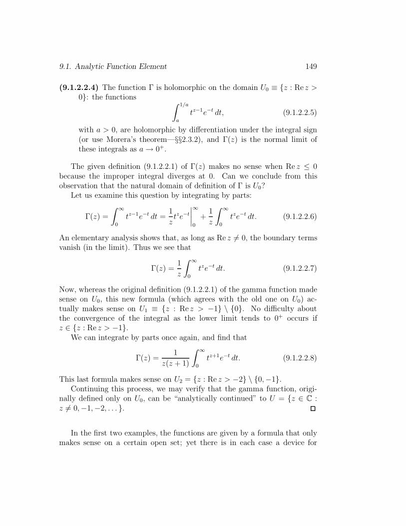
9.1. Analytic Function Element 149
(9.1.2.2.4) The function Γ is holomorphic on the domain U0 ≡ {z : Re z >0}: the functions ∫ 1/a
a
tz−1e−t dt, (9.1.2.2.5)
with a > 0, are holomorphic by differentiation under the integral sign(or use Morera’s theorem—§§2.3.2), and Γ(z) is the normal limit ofthese integrals as a→ 0+.
The given definition (9.1.2.2.1) of Γ(z) makes no sense when Re z ≤ 0because the improper integral diverges at 0. Can we conclude from thisobservation that the natural domain of definition of Γ is U0?
Let us examine this question by integrating by parts:
Γ(z) =
∫ ∞
0
tz−1e−t dt =1
ztze−t
∣∣∣∣∞
0
+1
z
∫ ∞
0
tze−t dt. (9.1.2.2.6)
An elementary analysis shows that, as long as Re z 6= 0, the boundary termsvanish (in the limit). Thus we see that
Γ(z) =1
z
∫ ∞
0
tze−t dt. (9.1.2.2.7)
Now, whereas the original definition (9.1.2.2.1) of the gamma function madesense on U0, this new formula (which agrees with the old one on U0) ac-tually makes sense on U1 ≡ {z : Re z > −1} \ {0}. No difficulty aboutthe convergence of the integral as the lower limit tends to 0+ occurs ifz ∈ {z : Re z > −1}.
We can integrate by parts once again, and find that
Γ(z) =1
z(z + 1)
∫ ∞
0
tz+1e−t dt. (9.1.2.2.8)
This last formula makes sense on U2 = {z : Re z > −2} \ {0,−1}.Continuing this process, we may verify that the gamma function, origi-
nally defined only on U0, can be “analytically continued” to U = {z ∈ C :z 6= 0,−1,−2, . . . }.
In the first two examples, the functions are given by a formula that onlymakes sense on a certain open set; yet there is in each case a device for
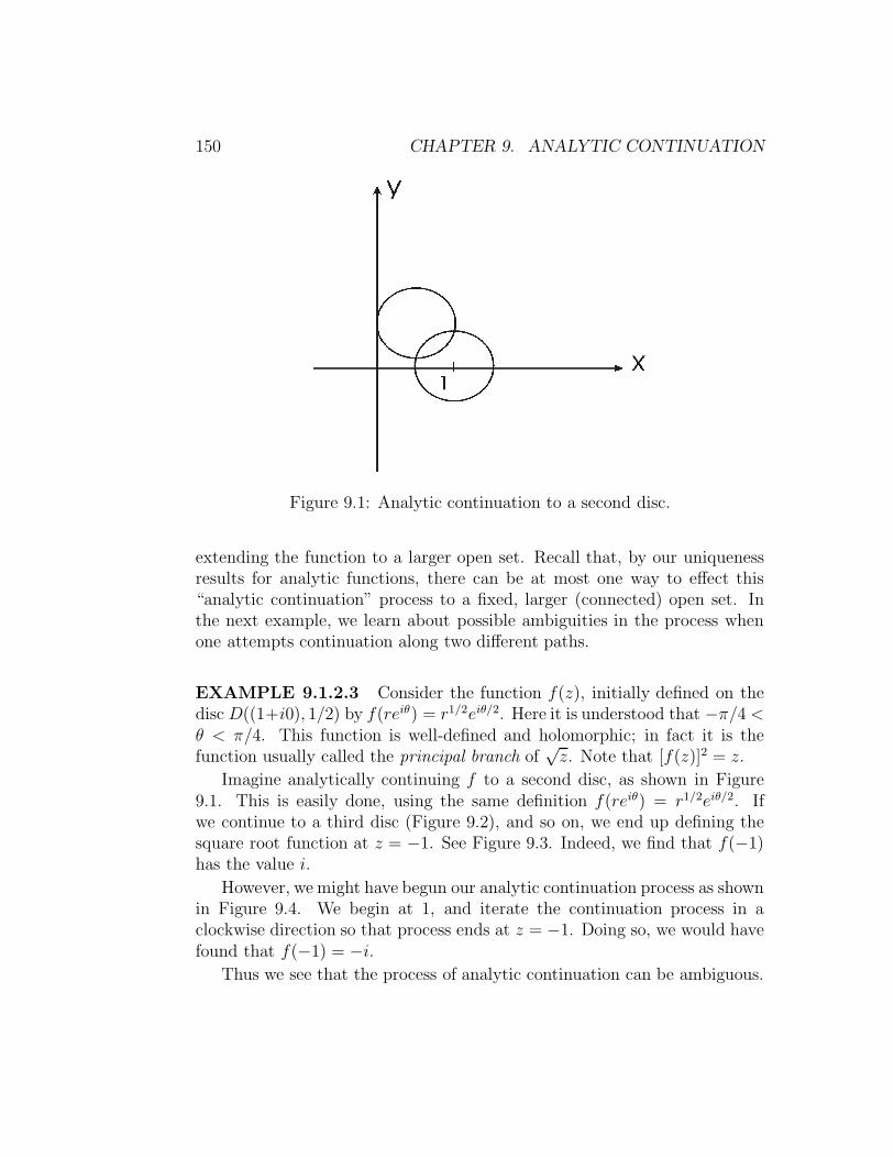
150 CHAPTER 9. ANALYTIC CONTINUATION
Figure 9.1: Analytic continuation to a second disc.
extending the function to a larger open set. Recall that, by our uniquenessresults for analytic functions, there can be at most one way to effect this“analytic continuation” process to a fixed, larger (connected) open set. Inthe next example, we learn about possible ambiguities in the process whenone attempts continuation along two different paths.
EXAMPLE 9.1.2.3 Consider the function f(z), initially defined on thedisc D((1+i0), 1/2) by f(reiθ) = r1/2eiθ/2. Here it is understood that −π/4 <θ < π/4. This function is well-defined and holomorphic; in fact it is thefunction usually called the principal branch of
√z. Note that [f(z)]2 = z.
Imagine analytically continuing f to a second disc, as shown in Figure9.1. This is easily done, using the same definition f(reiθ) = r1/2eiθ/2. Ifwe continue to a third disc (Figure 9.2), and so on, we end up defining thesquare root function at z = −1. See Figure 9.3. Indeed, we find that f(−1)has the value i.
However, we might have begun our analytic continuation process as shownin Figure 9.4. We begin at 1, and iterate the continuation process in aclockwise direction so that process ends at z = −1. Doing so, we would havefound that f(−1) = −i.
Thus we see that the process of analytic continuation can be ambiguous.

9.1. Analytic Function Element 151
Figure 9.2: Continuation to a third disc.
Figure 9.3: Analytic continuation of the square root function.

152 CHAPTER 9. ANALYTIC CONTINUATION
Figure 9.4: Analytic continuation in the other direction.
In the present example, the ambiguity is connected to the fact that a holo-morphic square root function cannot be defined in any neighborhood of theorigin; yet our two paths of analytic continuation encircle the origin.
It is because of the phenomena illustrated in these three examples—andmany others like them—that we must take a detailed and technical approachto the process of analytic continuation. Even making the questions them-selves precise takes some thought.
9.1.3 Function Elements
A function element is an ordered pair (f, U), where U is a disc D(P, r) and fis a holomorphic function defined on U . If W is an open set, then a functionelement in W is a pair (f, U) such that U ⊆ W .
9.1.4 Direct Analytic Continuation
Let (f, U) and (g, V ) be function elements. We say that (g, V ) is a directanalytic continuation of (f, U) if U ∩ V 6= ∅ and f and g are equal on U ∩ V(Figure 9.5). Obviously (g, V ) is a direct analytic continuation of (f, U) ifand only if (f, U) is a direct analytic continuation of (g, V ).
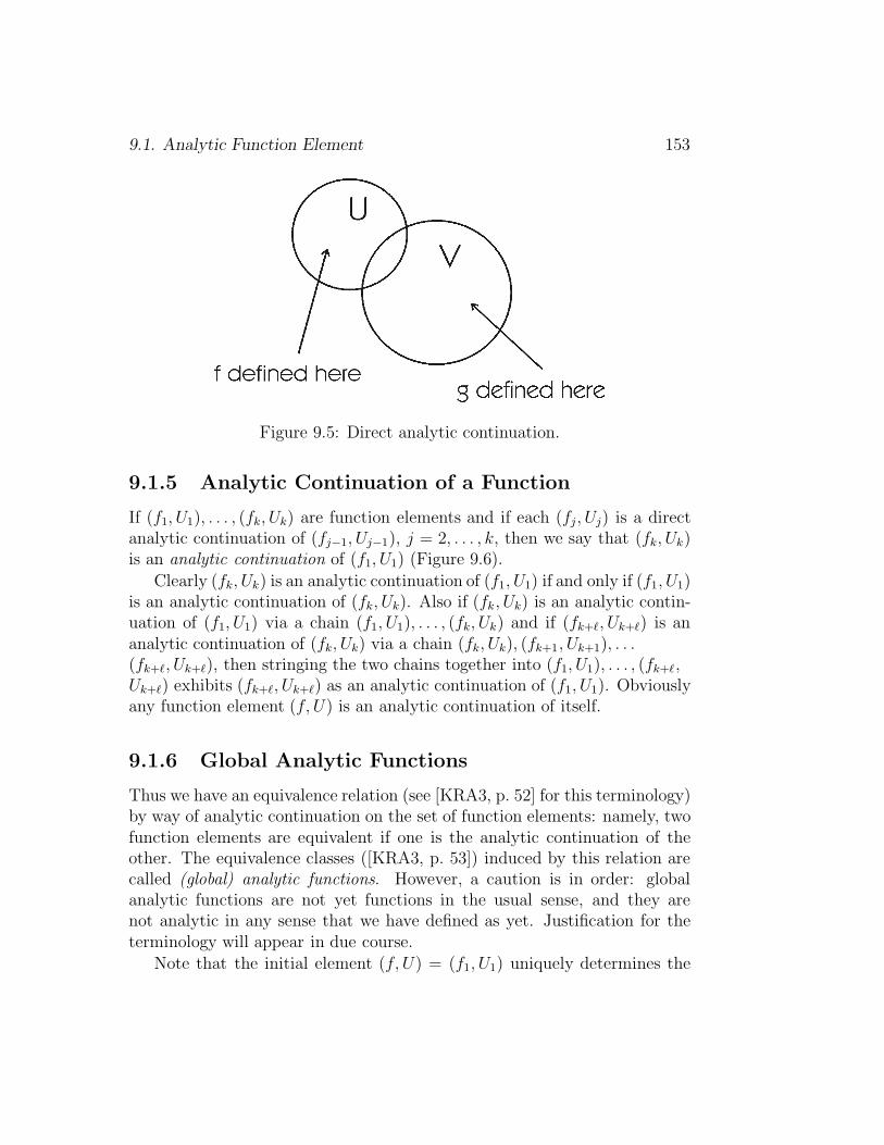
9.1. Analytic Function Element 153
Figure 9.5: Direct analytic continuation.
9.1.5 Analytic Continuation of a Function
If (f1, U1), . . . , (fk, Uk) are function elements and if each (fj, Uj) is a directanalytic continuation of (fj−1, Uj−1), j = 2, . . . , k, then we say that (fk, Uk)is an analytic continuation of (f1, U1) (Figure 9.6).
Clearly (fk, Uk) is an analytic continuation of (f1, U1) if and only if (f1, U1)is an analytic continuation of (fk, Uk). Also if (fk, Uk) is an analytic contin-uation of (f1, U1) via a chain (f1, U1), . . . , (fk, Uk) and if (fk+`, Uk+`) is ananalytic continuation of (fk, Uk) via a chain (fk, Uk), (fk+1, Uk+1), . . .(fk+`, Uk+`), then stringing the two chains together into (f1, U1), . . . , (fk+`,Uk+`) exhibits (fk+`, Uk+`) as an analytic continuation of (f1, U1). Obviouslyany function element (f, U) is an analytic continuation of itself.
9.1.6 Global Analytic Functions
Thus we have an equivalence relation (see [KRA3, p. 52] for this terminology)by way of analytic continuation on the set of function elements: namely, twofunction elements are equivalent if one is the analytic continuation of theother. The equivalence classes ([KRA3, p. 53]) induced by this relation arecalled (global) analytic functions. However, a caution is in order: globalanalytic functions are not yet functions in the usual sense, and they arenot analytic in any sense that we have defined as yet. Justification for theterminology will appear in due course.
Note that the initial element (f, U) = (f1, U1) uniquely determines the

154 CHAPTER 9. ANALYTIC CONTINUATION
Figure 9.6: Analytic continuation of a function element.
global analytic function, or equivalence class, that contains it. But a globalanalytic function may include more than one function element of the form(f, U) for a fixed disc U (see Example 9.1.2.3). Indeed, a global analyticfunction f may have in effect more than one value at a point: two functionelements (f1, U) and (f2, U) can be equivalent even though f1(P ) 6= f2(P ),where P is the center of the disc U . If f denotes the global analytic functioncorresponding to (f, U), then we call (f, U) a branch of f.
9.1.7 An Example of Analytic Continuation
EXAMPLE 9.1.7.1 Let U = D(1+ i0, 1/2) and let f be the holomorphicfunction log z. Here log z is understood to be defined to be log |z| + i arg z,and −π/4 < arg z < π/4. As in Example 9.1.2.3, the function element (f, U)can be analytically continued to the point −1 + i0 in (at least) two differentways, depending on whether the continuation is along a curve proceedingclockwise about the origin or counterclockwise about the origin.
In fact, all the “branches” of log z can be obtained by analytic continu-ation of the log |z| + iarg z branch on D(1 + 0i, 1/2) (by continuing severaltimes around the origin, either clockwise or counterclockwise). Thus the idea
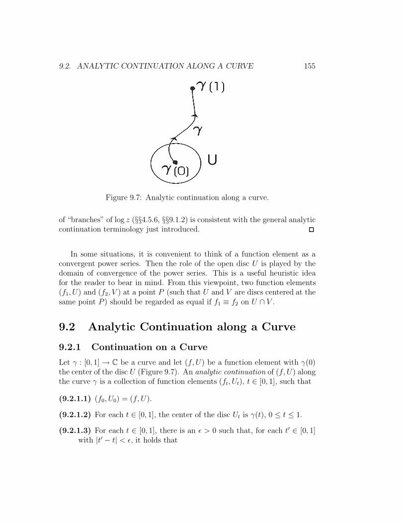
9.2. ANALYTIC CONTINUATION ALONG A CURVE 155
Figure 9.7: Analytic continuation along a curve.
of “branches” of log z (§§4.5.6, §§9.1.2) is consistent with the general analyticcontinuation terminology just introduced.
In some situations, it is convenient to think of a function element as aconvergent power series. Then the role of the open disc U is played by thedomain of convergence of the power series. This is a useful heuristic ideafor the reader to bear in mind. From this viewpoint, two function elements(f1, U) and (f2, V ) at a point P (such that U and V are discs centered at thesame point P ) should be regarded as equal if f1 ≡ f2 on U ∩ V .
9.2 Analytic Continuation along a Curve
9.2.1 Continuation on a Curve
Let γ : [0, 1] → C be a curve and let (f, U) be a function element with γ(0)the center of the disc U (Figure 9.7). An analytic continuation of (f, U) alongthe curve γ is a collection of function elements (ft, Ut), t ∈ [0, 1], such that
(9.2.1.1) (f0, U0) = (f, U).
(9.2.1.2) For each t ∈ [0, 1], the center of the disc Ut is γ(t), 0 ≤ t ≤ 1.
(9.2.1.3) For each t ∈ [0, 1], there is an ε > 0 such that, for each t′ ∈ [0, 1]with |t′ − t| < ε, it holds that

156 CHAPTER 9. ANALYTIC CONTINUATION
Figure 9.8: Direct analytic continuation.
(a) γ(t′) ∈ Ut and hence Ut′ ∩ Ut 6= ∅;
(b) ft ≡ ft′ on Ut′∩Ut (so that (ft, Ut) is a direct analytic continuationof (ft′, Ut′)). Refer to Figure 9.8.
Let (f, U) be a function element with U a disc having center P . Let γbe a curve such that γ(0) = P . Any two analytic continuations of (f, U)along γ agree in the following sense: if (fm, Um) is the terminal element of
one analytic continuation (ft, Ut) and if (f em, Uem) is the terminal element of
another analytic continuation (fet, Uet), then fm and f em are equal on Um∩ Uem.
9.2.2 Uniqueness of Continuation along a Curve
Thus we see that the analytic continuation of a given function element alonga given curve is essentially unique, if it exists. From here on, to avoid beingpedantic, we shall regard two analytic continuations (ft, Ut) and (ft, Ut) as
“equal,” or equivalent, if ft = ft on Ut∩ Ut for all t. With this terminologicalconvention (which will cause no trouble), the result of §9.2.1 says exactly thatanalytic continuation of a given function element along a curve is unique.

9.3. THE MONODROMY THEOREM 157
9.3 The Monodromy Theorem
The fundamental issue to be addressed in the present section is this:
9.3.1 Unambiguity of Analytic Continuation
Let P and Q be points in the complex plane. Let (f, U) be afunction element such that U is a disc centered at P . If γ1, γ2
are two curves that begin at P and terminate at Q then does theterminal element of the analytic continuation of (f, U) along γ1
equal the terminal element of the analytic continuation of (f, U)along γ2 (on their common domain of definition)?
We shall begin to answer this question in §§9.3.2. The culmination of ourdiscussion will be the monodromy theorem in §§9.3.5.
9.3.2 The Concept of Homotopy
Let W be a domain in C. Let γ0 : [0, 1] → W and γ1 : [0, 1] → W be curves.Assume that γ0(0) = γ1(0) = P and that γ0(1) = γ1(1) = Q. We say thatγ0 and γ1 are homotopic in W (with fixed endpoints) if there is a continuousfunction
H : [0, 1] × [0, 1] →W (9.3.2.1)
such that
(9.3.2.2) H(0, t) = γ0(t) for all t ∈ [0, 1];
(9.3.2.3) H(1, t) = γ1(t) for all t ∈ [0, 1];
(9.3.2.4) H(s, 0) = P for all s ∈ [0, 1];
(9.3.2.5) H(s, 1) = Q for all s ∈ [0, 1].
Then H is called a homotopy (with fixed endpoints) of the curve γ0 to thecurve γ1. Refer to Figure 9.9 to view two curves that are homotopic and twothat are not.

158 CHAPTER 9. ANALYTIC CONTINUATION
Figure 9.9: The concept of homotopy.
9.3.3 Fixed Endpoint Homotopy
Note: Since we are only interested in homotopies with fixed endpoints, weshall omit the phrase “with fixed endpoints” in the remainder of our discus-sion.
Intuitively, we think of a homotopy H as follows. Let Hs(t) = H(s, t).Then condition (9.3.2.2) says that H0 is the curve γ0. Condition (9.3.2.3)says that H1 is the curve γ1. Condition (9.3.2.4) says that all the curvesHs begin at P . Condition (9.3.2.5) says that all the curves Hs terminate atQ. The homotopy amounts to a continuous deformation of γ0 to γ1 with allcurves in the process restricted to lie in W .
We introduce one last piece of terminology:
9.3.4 Unrestricted Continuation
Let W be a domain and let (f, U) be a function element in W . We say (f, U)admits unrestricted continuation in W if there is an analytic continuation(ft, Ut) of (f, U) along every curve γ that begins at P and lies in W .

9.3. THE MONODROMY THEOREM 159
Figure 9.10: The concept of monodromy.
9.3.5 The Monodromy Theorem
One situation, in practice the primary situation, in which the question raisedin §§9.3.1 always has an affirmative answer is given by the following theorem:
The Monodromy Theorem: Let W ⊆ C be a connected openset. Let (f, U) be a function element with U ⊆ W . Let P denotethe center of the disc U . Assume that (f, U) admits unrestrictedcontinuation in W . If γ0, γ1 are each curves that begin at P ,terminate at some point Q, and are homotopic in W , then theanalytic continuation of (f, U) to Q along γ0 equals the analyticcontinuation of (f, U) to Q along γ1. Refer to Figure 9.10.
9.3.6 Monodromy and Globally Defined Analytic
Functions
Let W ⊆ C be a connected open set. Assume further that W is topologicallysimply connected, in the sense that any two curves that begin at the samepoint and end at the same point (possibly different from the initial point)are homotopic—see the related discussion of simple connectivity in §§2.3.3.Assume that (f, U) admits unrestricted continuation in W . Then there is aglobally defined holomorphic function F on W that equals f on U .
In view of the monodromy theorem, we now can understand specificallyhow it can be that the function
√z, and more generally the function log z,

160 CHAPTER 9. ANALYTIC CONTINUATION
cannot be analytically continued in a well-defined fashion to all of C\{0}. Thedifficulty is with the two curves specified in Example 9.1.2.3, or in Exampleof 9.1.7.1: they are not homotopic in the region C \ {0} (which is the regionof definition of the analytic function being considered).
9.4 The Idea of a Riemann Surface
9.4.1 What is a Riemann Surface?
In this section we give an intuitive description of the concept of what is calleda Riemann surface.
The idea of a Riemann surface is that one can visualize geometricallythe behavior of function elements and their analytic continuations. At themoment, a global analytic function is an analytic object. A global analyticfunction is the set of all function elements obtained by analytic continuationalong curves (from a base point P ∈ C) of a function element (f, U) atP . Such a set, which amounts to a collection of convergent power series atdifferent points of the plane C, does not seem very geometric in any sense.But in fact it can be given the structure of a surface, in the intuitive senseof that word, quite easily. (The precise definition and detailed definition ofwhat a “surface” is would take us too far afield: we shall be content herewith the informal idea that a surface is a two-dimensional object that locally“looks like” an open set in the plane. A more precise definition would bethat a surface is a topological space that is locally homeomorphic to C. See[LST], [ONE] for a more detailed discussion of surfaces.)
9.4.2 Examples of Riemann Surfaces
The idea that we need is most easily appreciated by first working with a fewexamples. Consider the function element (f, U) defined on U = D(1+0i, 1/2)by
z = reiθ 7→ r1/2eiθ/2, (9.4.2.1)
where r > 0 and −π/4 < θ < π/4 makes the reiθ representation of z ∈ D(1, 1)unique. This function element is the “principal branch of
√z ” at z = 1 that
we have already discussed in Example 9.1.2.3. The functional element (f, U)can be analytically continued along every curve γ emanating from 1 and lyingin C \ {0}. Let us denote by R (for “Riemann surface”) the totality of all

9.4. THE IDEA OF A RIEMANN SURFACE 161
function elements obtained by such analytic continuations. Of course, in set-theoretic terms, R is just the global analytic function
√z, just as we defined
this concept earlier in §§9.1.6. All we are trying to do now is to “visualize”R in some sense.
Note that every point of R “lies over” a unique point of C\{0}. A functionelement (f, U) ∈ R is associated to the center of U , that is to say, (f, U) isa function element at a point of C \ {0}. So we can define a “projection”π : R → C \ {0} by
π((f, U)) = the center of the disc U. (9.4.2.2)
This is just new terminology for a situation that we have already discussed.The projection π of R is two-to-one onto C \ {0}. In a neighborhood of a
given z ∈ C \ {0}, there are exactly two holomorphic branches of√z. [If one
of these is (f, U), then the other is (−f, U). But there is no way to decidewhich of (f, U) and (−f, U) is the square root in any sense that can be madeto vary continuously over all of C \ {0}.] We can think of R as a “surface”in the following manner:
Let us define neighborhoods of “points” (f, U) in R by declaring a neigh-borhood of (f, U) to be
{(fp, Up) : p ∈ U and (fp, Up) is a direct
analytic continuation of (f, U) to p}.
(9.4.2.3)
This new definition may seem formalistic and awkward. But it has the at-tractive property that it makes π : R → C \ {0} locally one-to-one. Every(f, U) has a neighborhood that maps, under π, one-to-one onto an open sub-set of C \ {0}. This gives a way to think of R as being locally like an openset in the plane.
Let us try to visualize R still further. Let W = C \ {z = x+ i0 : x ≤ 0}.Then π−1(W ) decomposes naturally into two components, each of which isan open set in R. (Since we have defined neighborhoods of points in R, wenaturally have a concept of open set in R as well.) These two componentsare “glued together” in R itself: R is connected, while π−1(W ) is not. Notethat, on each of the connected components of π−1(W ), the projection π isone-to-one. All of this language is just a formalization of the fact that, on

162 CHAPTER 9. ANALYTIC CONTINUATION
Figure 9.11: Forming a Riemann surface.
W , there are two holomorphic branches of√z—namely reiθ 7→ r1/2eiθ/2 and
reiθ 7→ −r1/2eiθ/2, −π < θ < π.
Each of the components of π−1(W ) can be thought of as a “copy” ofW , since π maps a given component one-to-one onto W . See Figure 9.11.How are these “copies,” say Q1 and Q2, glued together to form R? We jointhe second quadrant edge of Q1 to the third quadrant edge of Q2 and thesecond quadrant edge of Q2 to the third quadrant edge of Q1. Of coursethese joins cannot be simultaneously performed in three-dimensional space.So our picture is idealized. See Figure 9.12. Tacitly, in our construction ofR, we have restored the negative real axis.
9.4.3 The Riemann Surface for the Square Root Func-tion
We have now constructed a surface, known as the “Riemann surface for thefunction
√z.” This surface that we have obtained by gluing together the two
copies of W is in fact homeomorphic to the topological space that we madefrom R (the set of function elements) when we defined neighborhoods in R.So we can regard our geometric surface, built from gluing the two copies ofW together, and the function element space R, as being the same thing, thatis the same surface.
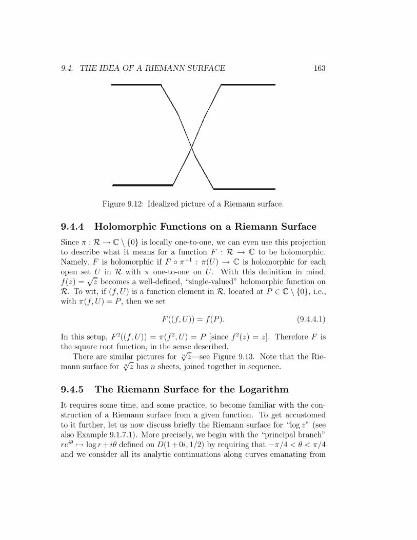
9.4. THE IDEA OF A RIEMANN SURFACE 163
Figure 9.12: Idealized picture of a Riemann surface.
9.4.4 Holomorphic Functions on a Riemann Surface
Since π : R → C \ {0} is locally one-to-one, we can even use this projectionto describe what it means for a function F : R → C to be holomorphic.Namely, F is holomorphic if F ◦ π−1 : π(U) → C is holomorphic for eachopen set U in R with π one-to-one on U . With this definition in mind,f(z) =
√z becomes a well-defined, “single-valued” holomorphic function on
R. To wit, if (f, U) is a function element in R, located at P ∈ C \ {0}, i.e.,with π(f, U) = P , then we set
F ((f, U)) = f(P ). (9.4.4.1)
In this setup, F 2((f, U)) = π(f2, U) = P [since f2(z) = z]. Therefore F isthe square root function, in the sense described.
There are similar pictures for n√z—see Figure 9.13. Note that the Rie-
mann surface for n√z has n sheets, joined together in sequence.
9.4.5 The Riemann Surface for the Logarithm
It requires some time, and some practice, to become familiar with the con-struction of a Riemann surface from a given function. To get accustomedto it further, let us now discuss briefly the Riemann surface for “log z” (seealso Example 9.1.7.1). More precisely, we begin with the “principal branch”reiθ 7→ log r+ iθ defined on D(1+0i, 1/2) by requiring that −π/4 < θ < π/4and we consider all its analytic continuations along curves emanating from

164 CHAPTER 9. ANALYTIC CONTINUATION
Figure 9.13: The Riemann surface for n√z.
1. We can visualize the “branches” here by noting that, again with W =C\({0}∪ the negative real axis), π−1(W ) has infinitely many components—each a copy of W—on which π maps one-to-one onto W . Namely, thesecomponents are the “branches” of log z on W :
reiθ 7→ log r + iθ + 2πik, k ∈ Z, (9.4.5.1)
where −π < θ < π. Picture each of these (infinitely many) images stackedone above the other (Figure 9.14). We join them in an infinite spiral, orscrew, with the upper edge of the kth surface being joined to the lower edgeof the (k − 1)st surface. Observe that going around the origin (countedclockwise in C \ {0}) corresponds to going around and up one level on thespiral surface. This is the geometric representation of the fact that, whenwe analytically continue a branch of log r+ iθ+ 2πik once around the origincounterclockwise then k increases by 1. This time there is no joining of thefirst and last “sheets.” The spiral goes on without limit in both direction.
9.4.6 Riemann Surfaces in General
The idea that we have been discussing, of building surfaces from functionelements, can be carried out in complete generality: Consider the set of allanalytic function elements that can be obtained by analytic continuation(along some curve in C) of a given function element (f, U). This is what wecalled earlier a global analytic function. Then this set of function elements

9.5. PICARD’S THEOREMS 165
Figure 9.14: The Riemann surface for logarithm.
can actually (and always) be regarded as a connected surface: There is aprojection onto an open set in C obtained by sending each function element tothe point of C at which it is located. This projection is a local identificationof the set of function elements with part of C, and so it in effect exhibitsthe set of function elements as being two-dimensional, i.e., a surface; afterthis observation, everything proceeds as in the examples. The reader isinvited to experiment with these new ideas—see particularly the discussionand exercises in [GK].
9.5 Picard’s Theorems
9.5.1 Value Distribution for Entire Functions
The image, or set of values, of an entire function must be quite large. Thisstatement is true in a variety of technical senses, and Nevanlinna theory givesa detailed development of the concept. Here we simply enunciate the theo-rems of Picard which give some sense of the robustness of entire functions.
9.5.2 Picard’s Little Theorem
Theorem: If the range of a holomorphic function f : C → C
omits two points of C, then f is constant.
166 CHAPTER 9. ANALYTIC CONTINUATION
The entire function f(z) = ez shows that an entire function can omit onevalue (in this case, the value 0). But the theorem says that the only waythat it can omit two values is if the function in question is constant.
9.5.3 Picard’s Great Theorem
The following theorem, known as the great theorem of Picard, strengthensthe Little Theorem (see §§9.5.4 for the explication of this connection).
Theorem: Let U be a region in the plane, P ∈ U, and supposethat f is holomorphic on U \{P} and has an essential singularityat P . If ε > 0, then the restriction of f to U ∩ [D(P, ε) \ {P}]assumes all complex values except possibly one.
9.5.4 The Little Theorem, the Great Theorem, and
the Casorati-Weierstrass Theorem
Compare Picard’s great theorem with the Casorati/Weierstrass theorem (§§4.1.6).The Casorati/Weierstrass theorem says that, in a deleted neighborhood of anessential singularity, a holomorphic function assumes a dense set of values.Picard’s theorem refines this to “all values except possibly one.”
What is the connection between the great theorem and the little theorem?And how do these two theorems relate to the results about entire functionsthat we have already seen?
A non-constant entire function cannot be bounded near infinity, or elseit would be bounded on C and hence (by Liouville’s theorem—§§3.1.3) beconstant. So it has either a pole or an essential singularity at infinity. Inthe first instance, the function is a polynomial (see §§4.6.6). But then theFundamental Theorem of Algebra (§§1.1.7) tells us that the function assumesall complex values. In the second instance, the great theorem applies at thepoint ∞ and implies the little theorem.
Nevanlinna theory is an analytic refinement of the ideas we have beendiscussing here. There is a delicate interplay between the rate of growth (at∞) of an entire function and the distribution of its zeros.

Bibliography
[BKR] B. E. Blank and S. G. Krantz, Calculus, Key College Press,Emeryville, CA, 2006.
[OH] R. Courant and D. Hilbert, Methods of Mathematical Physics,Wiley-Interscience, New York, 1953.
[GAR] J. B. Garnett, Bounded Analytic Functions, Academic Press, NewYork, 1981.
[GRK] R. E. Greene, and S. G. Krantz, Function Theory of One ComplexVariable, 2nd ed., American Mathematical Society, Providence, RI,2002.
[HER] I. Herstein, Topics in Algebra, Blaisdell, New York, 1964.
[HES] Z. He and O. Schramm, Koebe uniformization and circle packing,Ann. of Math. 137(1993), 369–4013.
[HUN] T. W. Hungerford, Algebra, Springer-Verlag, New York, 1998.
[KRA1] S. G. Krantz, A Panorama of Harmonic Analysis, MathematicalAssociation of America, Washington, D.C., 1999.
[KRA2] S. G. Krantz, Complex Analysis: The Geometric Viewpoint, 2nd
ed., Mathematical Association of America, Washington, D.C.,2004.
[KRA3] S. G. Krantz, Real Analysis and Foundations, 2nd ed., CRC Press,Boca Raton, FL, 2005.
167

168 References
[KRA4] S. G. Krantz, Cornerstones of Geometric Function Theory: Ex-plorations in Complex Analysis, Birkhauser Publishing, Boston,2006.
[KRA5] S. G. Krantz, Function Theory of Several Complex Variables, 2nd
ed., American Mathematical Society, Providence, RI, 2001.
[KRA6] S. G. Krantz, Complex Variables: A Physical Approach with Ap-plications and MatLab, Taylor & Francis, Boca Raton, FL, 2008.
[LOG] J. D. Logan, Applied Mathematics, 2nd ed., John Wiley and Sons,New York, 1997.
[RUD1] W. Rudin, Principles of Mathematical Analysis, McGraw-Hill,New York, 1953.

Index
169