210-1

A Gradient-free Approach to Inverse-conditioning of Heterogeneous Reservoir Models to Pressure Data

Dan K. Khana, Clayton V. Deutschb and C.A. Mendozaa

a Department of Earth & Atmospheric Sciences,

b Centre for Computational Geostatisitics University of Alberta

The inverse problem of estimating the effective permeability over a heterogeneous reservoir or aquifer from pressure or hydraulic head data has been tackled by various approaches over the last few decades. This paper presents a considerably more straightforward approach than what has been usually presented on this topic.

The gradient-free calibration method works without the need for expensive or technically-involved computations of sensitivity coefficients and the associated gradient of the model response with respect to the parameters. A simple and effective approximation procures a matrix of sensitivity indicators as a substitute for the computation of the Jacobian matrix. A rules-based approach for determining the required parameter sensitivity information is based upon: (1) delineation of flowpaths relevant to the calibration head data, (2) transforming the permeability field into a categorical variable in order to define relatively high-transmissivity and low-permeability geobodies, and (3) identification of geobody connections to fluid sources or sinks in the model. Parameter optimization is based on the deterministic gradient information inferred from the sign on the sensitivity coefficients and the head mismatch at each calibration point. The optimization algorithm uses an approximation of the gradient of the model response with respect to the parameters that is adapted from a proven gradient-free optimization technique (SPSA).

The gradient-free method solves the inversion problem in a similar manner as proven gradient-based calibration methods, but with a much more transparent approach. As a result, we are able to elucidate some key points with respect to the inverse conditioning to head data, including the controls on the information available from a given configuration of head data in identifying important heterogeneity features controlling the flow response. Specifically: key heterogeneities which impact the flow response must be sampled by the calibration data. A calibration data point “samples” a heterogeneity feature when it occurs along a flowline that intersects the feature. By this approach, the permeability field can be adjusted within sensitive areas, seeding spatially precise perturbations to produce a head match at that calibration data location which results in an improvement in the local precision of the spatial uncertainty model from the conditioning process.

Introduction and Background

Inverse modeling generally refers to identifying a model which adequately represents the system under analysis. Model identification is a broader and less frequently approached topic than parameter estimation, so more practically speaking, inverse modeling involves estimating the model parameters subject to the constraint that the model reproduces measurements of the system response. In particular, for aquifer and petroleum reservoir characterization, inverse modeling refers to estimating the model parameters based on measurements of fluid pressure, flow rates at

210-2

wells, tracer concentrations over time, and so on. These measurements are referred to as dynamic data, or calibration data, and are distinct from measurements of the properties represented by the parameters, which are complementarily called static data.

The problem of integrating dynamic data into geological models for aquifer and reservoir characterization remains an important area despite decades of research (Emsellem and de Marsily, 1971; Kitanidis and Vomvoris, 1983; Carrera and Neuman, 1986; RamaRao et al., 1995; Gomez-Hernandez et al., 1997; Medina and Carrera, 2003). Integrating dynamic data requires solving an inverse problem where the solution consists of model parameter estimates that result in a reproduction of these data via the model response. The ultimate goal of inverse flow modeling is to identify important heterogeneities of the distributed parameter field, most often the permeability, of a heterogeneous aquifer or reservoir in order to increase the predictive ability of the model by narrowing the spaces of uncertainty of the response variables.

Inverse conditioning refers to a posterior calibration of an ensemble of realizations (i.e., a model of spatial uncertainty) of the permeability field to dynamic data. The conditioning process must somehow address the complex non-linearity between the model response, as processed through a transfer function, typically a flow simulator, and the estimated model parameters. The initial suite of realizations may have been generated conditional to static rock property data such as transmissivity estimates based on well tests. However, in general, they will not permit a simulated reproduction of the available pressure or head measurements, resulting in poor predictive ability of the flow models. One major reason for this is because they fail to identify key heterogeneities that affect the flow system response.

This paper presents a gradient-free approach to inverse conditioning of stochastic models of aquifer or reservoir permeability. The method is based on an approximate prediction of the sensitivity of hydraulic head response to perturbations in the permeability field. Typically these sensitivity coefficients are obtained through expensive numerical procedures based on analytical formulations for parameter sensitivity (Carrera et al., 1990; Oliver, 1994, Chu et al., 1995, Carrera et al., 1997; Landa et al., 1997). In the gradient-free approach, parameter sensitivities are predicted, approximately, based on a set of physical criteria. This sensitivity approximation and an approximation of the associated gradient of the model response with respect to the parameters constitute a simplified methodology that offers several advantages over traditional gradient-based approaches. These advantages include: (1) a reduction in computational expense and computer code development effort; and (2) a clear understanding of the calibration process and the effects of conditioning to a given spatial configuration of calibration data.

The methodology presented in this paper utilizes and build upon the concepts of Sequential Self Calibration (Gomez-Hernandez et al., 1997), and Pilot Points (RamaRao et al., 1995). Earlier research tended to focus on understanding and dealing with the difficulties associated with the inverse problem in aquifer and reservoir identification, and the above-mentioned works are perhaps the pinnacle of that stage. Sequential Self Calibration (SSC) provided important conceptual advancements in solving the inverse problem in hydrogeology and reservoir characterization (Gomez-Hernandez et al., 1997; Capilla et al., 1997; Capilla et al., 1999; Wen et al., 1999). Through a combination of elements — mainly Geostatistics-based — this method has addressed difficulties associated with obtaining satisfactory solutions to the generally ill-posed, and consequently unstable solution methods to the inverse problem (de Marsily et al., 2000). The SSC concept is adopted as a framework for the gradient-free algorithm presented here.

210-3

Methodology

Synthetic examples are used to illustrate the gradient-free algorithm and to demonstrate the amount of information that can, in general, be expected from specific configurations of calibration head data with respect to identification of key heterogeneities. Synthetic examples assume a reference permeability field to be the “geological truth” and the calibration data are taken as a subset of the model response on that true field. The value of synthetic modeling studies is in the controlled experimental conditions, which permit the study to focus on key aspects of the modeling in order to illustrate foundational concepts.

Assumptions

he inversion problem to be solved is that of estimating the value of absolute permeability at each model cell in a two-dimensional flow system by calibration to a set of steady-state heads. Steady-state flow in a two dimensional domain of uniform thickness is considered. The flow model is expressed as:

Qgy

hkyx

hkx ρ

μ=⎟⎟

⎠

⎞⎜⎜⎝

⎛∂∂

∂∂

+⎟⎠⎞

⎜⎝⎛

∂∂

∂∂

, (1)

where h is the total hydraulic head, which for a horizontal model, taking the value at the center of the grid cells, is interchangeable with fluid pressure, but for generality, we use hydraulic head from this point; k is isotropic absolute permeability, Q is the sum of fluid sources and sinks over the domain; � and � are dynamic viscosity and density of the single fluid phase, respectively; and g is gravitational acceleration. The flow model is discretized by finite differences. The consideration of two dimensions is purely for convenience and simplicity. Neither the calibration algorithm, nor the concepts discussed are limited to two-dimensional applications. The assumption of steady state is made for simplicity and clarity of analysis and presentation.

The calibration data are obtained by solving the flow equations on a reference permeability field with the boundary conditions known exactly. The forward flow problem that is solved during the iterative calibration procedure uses exactly the same boundary conditions1, internal fluxes, grid discretization, iterative solver parameters, and so on. The spatial discretization of the model is assumed to be adequate with respect to resolving the heterogeneity that is relevant to the model response.

The spatial structure of the permeability field is assumed to be known insofar as the random function model that characterizes it. Thus, the only effective source of uncertainty is the parameter uncertainty due to the heterogeneity of the permeability field. The initial permeability realizations are unconditional. No static data is assumed available. This allows us to isolate the effects of conditioning to the head data.

The parameter perturbations are based on a multi-Gaussian model the propagation of optimal parameter perturbations throughout the domain is based on kriging. These assumptions are made for convenience. The focus of this paper, with respect to the calibration algorithm, is the gradient-free method. Any stochastic model could be implemented for the generation of initial parameter

1 Note that specified heads don’t assume perfectly known boundary conditions because the fluxes aren’t constrained. However, the results did not change significantly when exact reference fluxes were used (other than getting more correct magnitudes due to the steady state models).

210-4

field realizations with a consistent mechanism used for the generation and propagation of parameter perturbations.

Gradient-free calibration

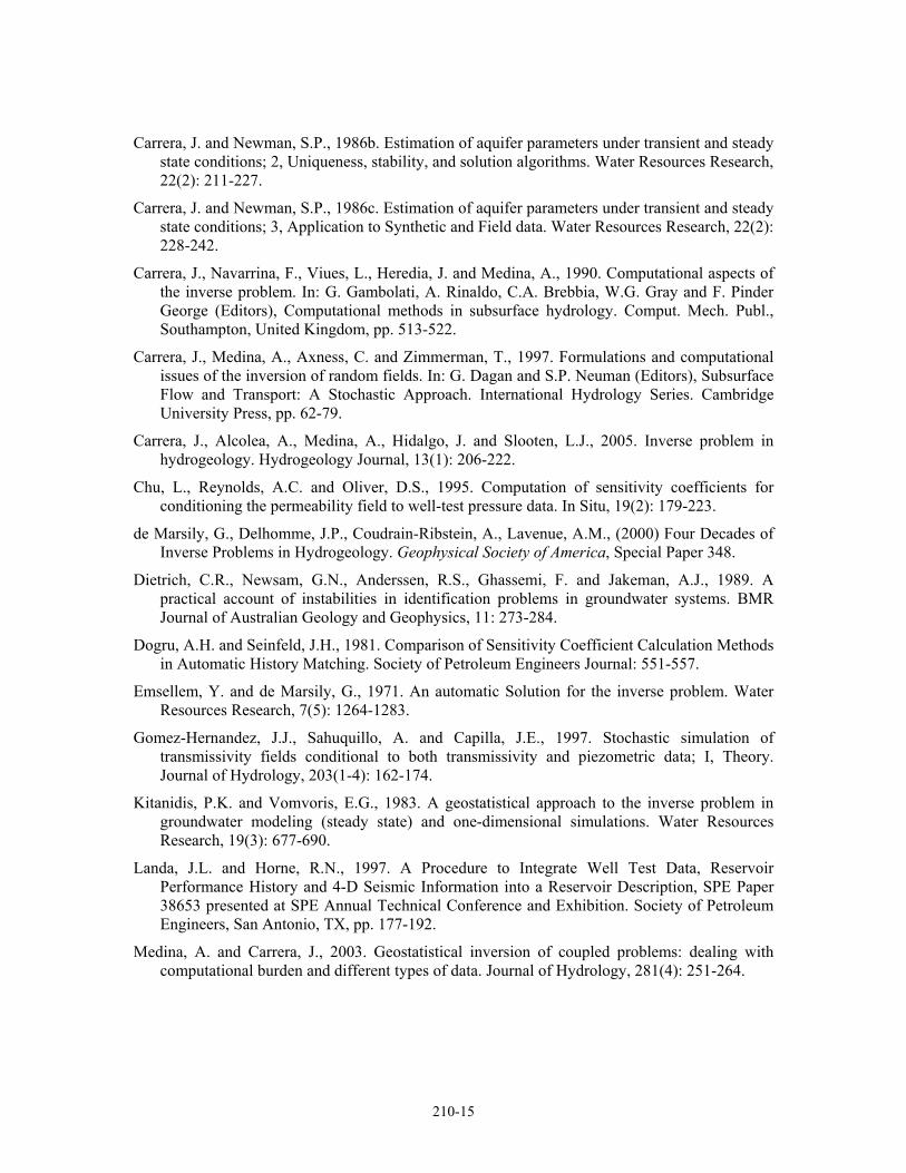
The algorithm structure is based on the SSC concept (Figure 1). It is an indirect calibration procedure that iteratively updates the parameter field until a satisfactory match to the head data is achieved. An outer loop consists of solving for head on the current realization and calculating the head mismatch between the model and the measured data. Unless the head mismatch is smaller than a specified tolerance, the algorithm proceeds with an inner parameter optimization routine (Figure 1).

In the gradient-free method, the calibration process begins by efficiently mapping sensitive areas of the model domain with respect to the calibration data locations. This step substitutes a system of sensitivity indicators for the calculation of sensitivity coefficients and constrains the randomized drawing of a parameter subset for optimization. For each calibration data location, a subset of model cells is drawn within sensitive regions of the model (Figure 1). The gradient-free optimization routine calculates perturbations to this parameter subset that will minimize the mismatch between the model-predicted head response and the measured data at the calibration locations. An inexpensive function evaluation is used which is based on a linear approximation of the model response about the proposed parameter changes (Gomez Hernandez et al., 1997). The perturbations are then propagated through the domain by a kriging of the optimal values. The permeability field is finally updated by addition of the resultant perturbation field to the current realization of the permeability field (Figure 1).

The elements that differentiate this gradient-free algorithm from SSC and other gradient-based approaches in general are:

(1) The calculation of the full matrix of sensitivity coefficients is done by a simple approximation.

(2) The parameterization scheme for the optimization is based on prior sensitivity information, which results in a “smart” selection of a subset of parameters to use in the optimization.

(3) The optimization routine is based on the Simultaneous Perturbation Stochastic Approximation (SPSA) method (Spall, 1992; 2003). The algorithm uses an approximation of the gradient of the objective function that is directly compatible with the approximate system of sensitivity indicators replacing the calculation of Jacobian matrix.

These three elements comprise the gradient-free approach and are explained in detail next.

Approximate sensitivities

Sensitivity coefficients are the partial derivatives of the model response at a location, j, with respect to a parameter change at model cell, i. We consider the sensitivity of head to the logarithm of permeability. The complete matrix of sensitivity coefficients, otherwise called the Jacobian matrix, may be expressed as:

mjNikth

sJi

jji ,...1;,...1,

)ln()(

}{ , ==∂

∂== (2)

210-5

where h is hydraulic head at a specific calibration data location and k is the effective permeability specified at a model cell.

Sensitivity coefficients are used to determine the search direction within the parameter space that results in an improved match between the calibration data and the model response (Carrera et al., 2005). However, the computational burden of calculating sensitivity coefficients has always been a limiting factor in the practicality of automated calibration algorithms (Carrera et al., 1990, 2005; Medina and Carrera, 2003).

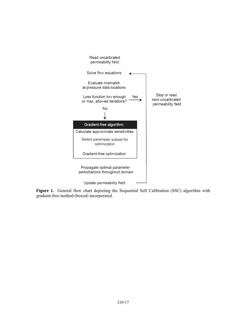
As an alternative to calculating the Jacobian matrix, an approximate system of sensitivity indicators may be obtained immediately following the head solution (Khan et al., this issue). The permeability structure coupled with the model specifications control the sensitivity of the model response at specific locations to perturbations of the permeability field. Sensitivity at a given calibration location is greatest to perturbations of permeability along streamlines intersecting that response location; particularly within relatively high transmissivity geobodies or features forming relatively low permeability barriers to flow (Figure 2). In order to quantify important permeability contrasts, a binary geobody classification scheme can be defined based on the selection of appropriate threshold permeability values2 (Figure 2b,c).

The criteria to predict sensitivity are: (1) cells that occur along flowpaths which intersect the locations of calibration data will be the most sensitive cells within the model (Figure 2d), with the additional constraints that; (2) they constitute geobodies of relatively high-transmissivity which are connected to a source or sink in the domain [Figure 2e; geobodies (ii-v)], or; (3) they are cells of relatively low permeability, forming hydraulic barriers [Figure 2e; geobody (i)]. Lastly, (4) the sign of the sensitivity coefficient is related to whether a model grid cell is located up- or downgradient from the observation location along a flowpath. Cells that are downgradient will always have a negative sign (Figure 2e).

A simple rules-based algorithm based on the above criteria is used to obtain a sensitivity indicator matrix comprised of zeros and 1’s, where non-zero elements indicate sensitive parameters. This indicator matrix approximates the form of the Jacobian matrix and can be used in place of the Jacobian in an appropriately-designed optimization routine (Khan et al., this issue). From this indicator matrix we obtain: (1) grid blocks with permeability values that are sensitive to the model response at a particular calibration location, and (2) the sign on the sensitivity (Figure 2e), which is critical to establishing the updating direction in the parameter optimization.

Parameterization

Given the extremely large number of parameters in the distributed parameter fields that populate flow model girds or meshes, an appropriate parameterization is needed for a well-posed optimization. The original SSC method utilizes a parameterization technique whereby a randomly-sampled subset of parameters is used in the optimization. This set of “master points” is 2 Remark: When defining the categorical variable for modeling geobodies it may be better to use an upper and a lower cutoff, resulting in three categories: (i) above the upper threshold, (ii) below the lower threshold, and (iii) between the two cutoff values. Only cells of categories (i) and (ii) will be potentially sensitive. In addition, for transient flow problems, it may be effective to define a different (pair of) threshold value(s) at given times in the simulation. For example, as time progresses and the flow response approaches equilibrium, increasingly low permeability values will be needed to constitute sensitive flow barriers. But the performance of the algorithm in the synthetic examples was not found to be highly sensitive to the cutoffs used in the definition of the geobody categories (as long as they do not become overly restrictive or all-inclusive).

210-6

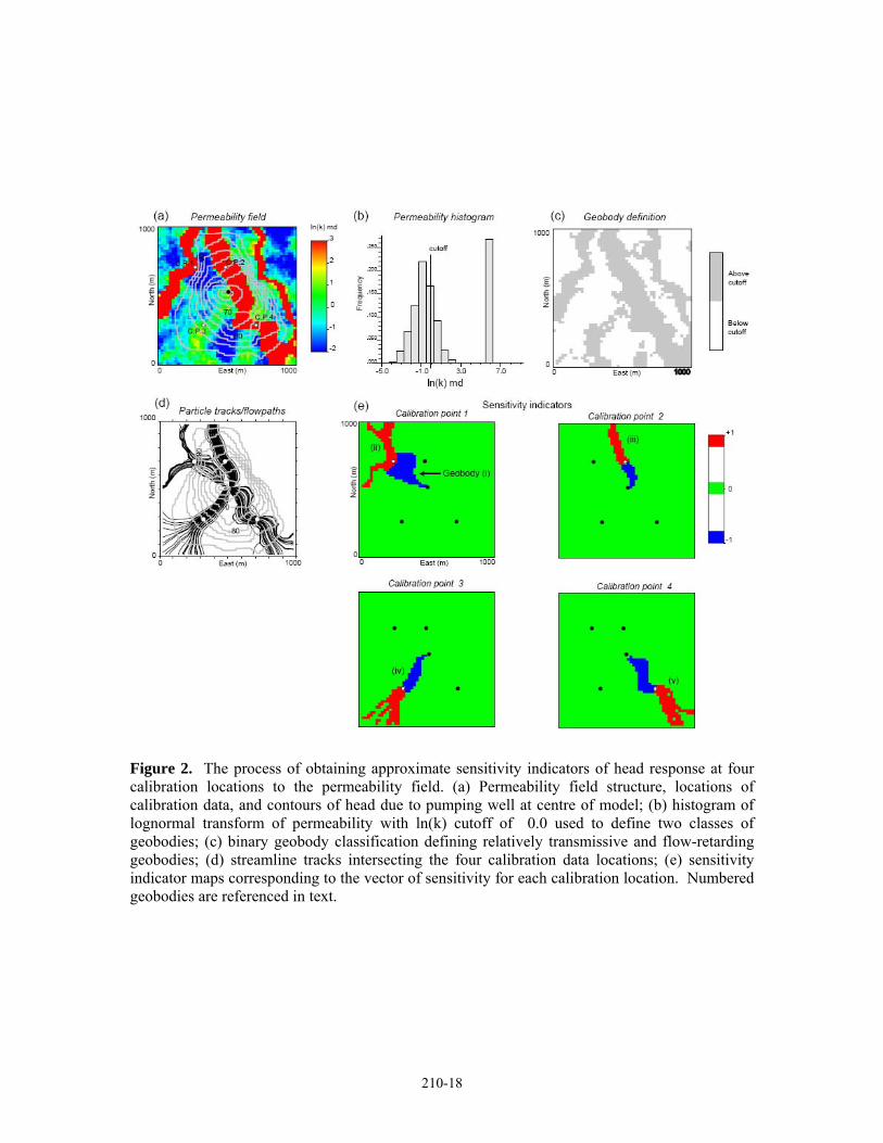
also used in the calculation of a parameterized Jacobian matrix, which is a clever way of reducing the computational burden of obtaining the full matrix of sensitivity coefficients. However, this parameterization scheme is not based on any sensitivity information, making it a “blind” approach.

The original SSC algorithm draws a set of master points using a random stratified sampling scheme in order to cover all of the zones or sub regions of the model, regardless of whether the head response at the calibration locations is sensitive to permeability at the master point locations or not (Figure 3a). In the gradient-free approach, a prior prediction of sensitivity of head to permeability, as described above, constrains the random drawing of a subset of parameters to use in the optimization (Figure 3b). This ensures that each of optimized permeability perturbations will effect a response at the calibration data locations. This parameterization scheme is a critically-important element of the gradient-free method — parameters with maximum sensitivity information are always selected, and each parameter carries information about the gradient of the model response, which leads directly to the gradient-free optimization method described next.

Gradient-free optimization

Gradient-based optimization methods are based on the evaluation of the gradient, g(θ) of a loss function, L(θ) with respect to the parameters, θ = [k1,k2,…,kM]T such that

( )

⎥⎥⎥⎥⎥⎥

⎦

⎤

⎢⎢⎢⎢⎢⎢

⎣

⎡

∂∂

∂∂

∂∂

=∂∂

≡

MkL

kL

kL

Lg 2

1

θθ . (3)

In the original SSC formulation, L(θ) and g(θ) are evaluated based on a linear approximation of the model response about the parameters (Gomez Hernandez et al., 1997). The evaluation of g(θ) depends on the calculation of the Jacobian matrix3.

Gradient-free methods work without the need for calculating the gradient of the loss function. Simultaneous Perturbation Stochastic Approximation (SPSA) is an algorithm that is based on a gradient approximation (Spall, 1992; 2003). The form of the SPSA gradient approximation is well-suited to an optimization using the sensitivity indicator matrix described previously.

The SPSA gradient approximation is typically evaluated using only two measurements of L(θ) about a simultaneous perturbation of the parameters. However, there is a one-sided approximation that may suitable for certain applications, which makes use of only one loss function measurement (Spall, 2003). The one-sided gradient approximation has the form,

3 In general, calculating g(θ) depends on the Jacobian. In SSC, calculation of L(θ) depends on the sensitivity matrix for the set of master points used.

210-7

( )( )

( )⎥⎥⎥⎥⎥⎥

⎦

⎤

⎢⎢⎢⎢⎢⎢

⎣

⎡

±

±

=

Ml

ll

l

ll

ll

ccL

ccL

g

ΔΔ

ΔΔ

θ

θ

θˆ

ˆ

ˆˆ1

, (4)

where cl is a positive scalar whose value at iteration l is given by a gain sequence satisfying certain well-known stochastic approximation conditions (Spall, 1992; 1998; 2003) and � is a mean-zero perturbation vector with a distribution that should satisfy certain specific conditions requiring bounded inverse moments for the elements of Δ (Spall, 2003). One commonly-used distribution which satisfies these conditions is a symmetric Bernoulli ± 1 distribution. Most of the rows of the sensitivity indicator matrix — where a row constitutes the vector of sensitivities for one calibration location (e.g., Figure 2e) — tend to follow this distribution4.

The gradient approximation in Equation (4) is designed to perform a stochastic search of the gradient space of a noisy loss function, or one that is costly to evaluate. However, for the problem of calibration to head data, Equation (4) can be used in a deterministic sampling of the gradient space. The sampling is deterministic in the sense that it can be known in advance from the head mismatch at a given calibration location whether an increase or a decrease in the elements of θ are needed to reduce the value of L(θj, where L(θ) is evaluated for each jth calibration data location.

The loss function is constructed based on the form of the SPSA gradient approximation and an expression for the linearization of the model response about the parameter perturbations. The gradient-free loss function is evaluated as

( ) oj

linjj hhL −=θ , (5)

where hjlin, the linear approximation of hydraulic head at the jth calibration point, is calculated as

a truncated series about the model-calculated head, hjc, on the current permeability field:

[ ]∑=

±+=M

iijli

cj

linj ckhh

1)ln( Δ , (6)

Note that in Equation (6), the term in the summation has the same form as the argument in the numerator of the elements of the SPSA gradient approximation5 (Equation 4). The ± 1 sensitivity indicators at the locations of the parameters to be optimized comprise the perturbation vector, Δ, and the scalar gain coefficient acts as a relaxation factor such that the products, cΔ, in Equation (6) behave like traditional sensitivity coefficients6. This apparently strange approach to

4 Even if some do not (i.e., very asymmetric with non-zero mean due to all negative or all positive sensitivities) this does not appreciably degrade the performance of the SPSA optimization. 5 The numerator is the same for all the elements in Equation (4); it is the value of the loss function at the current inner optimization iteration. This may be worth mentioning to reduce the possibility of confusion. 6 Aside from setting the seed value of this gain sequence following SPSA guidelines, you can check the optimization results after one outer iteration (a single SPSA run) to help tune an appropriate magnitude to the approximate sensitivities, cΔij by checking for reasonable magnitudes of the optimized perturbations.

210-8

approximating the Jacobian is really quite intuitive. Recall that what is obtained from the sensitivity indicator matrix is a binary map of sensitivities with respect to each calibration location (Figure 2e), indicating the sensitive areas of the model and the correct sign on the sensitivity of model response with respect to the parameters. The precise values of these approximate sensitivities are not important in the evaluation of the loss function by Equations (5) and (6); only approximately-correct magnitudes are needed since the most critical sensitivity information is already established.

The parameter vector θ is updated at each iteration using the general recursive form:

( )lllll ga θθθ ˆˆ1 −=+ , (7)

where al is a nonnegative scalar gain coefficient (Spall, 1992; 1998; 2003), which behaves like a relaxation factor, limiting the updating step size.

The main reason for using a multi-objective formulation (Equation 5) is that the parameter update direction is based on the sensitivity information and the head mismatch at each respective calibration location.

As an example, consider the case where the head mismatch (hc - ho) at a single calibration location is equal to -11 m, indicating that the calculated model response, hc, is below the observed value, ho, at that location (Figure 4). In order to reduce the mismatch, permeability must be reduced in areas of negative sensitivity coefficients and/or increased at locations having positive sensitivity with respect to this calibration location (Table 1). The subset of permeability values selected for optimization (Figure 4) are the initial M elements corresponding to 0̂θ in Equation (4), and the elements of the perturbation vector, Δ, correspond to the ±1 sensitivity indicators at those locations Table 1 The term in brackets in Equation (6) represents the proposed parameter updates for the lth iteration (Table 1). In the opposite case of a positive head mismatch at the calibration data location, Table 2 summarizes the direction of required changes to the parameters and the corresponding expression for the loss function evaluation considering the same parameterization (Figure 4).

Upon converging to a minimum loss function tolerance or reaching a maximum number of inner iterations, the optimal parameter perturbation vector is propagated through the domain by kriging (Figure 1).

Results and discussion

This section has two parts: (1) a demonstration of the algorithm working to condition prior realizations of the permeability structure of two synthetic reservoirs; and (2) a discussion on the identification of the key heterogeneities through inverse conditioning to head data. The second part, on identification, is a general topic of importance to inverse modeling of heterogeneity using dynamic data. However, the elements of the gradient-free method make clear what to expect from the inverse conditioning process.

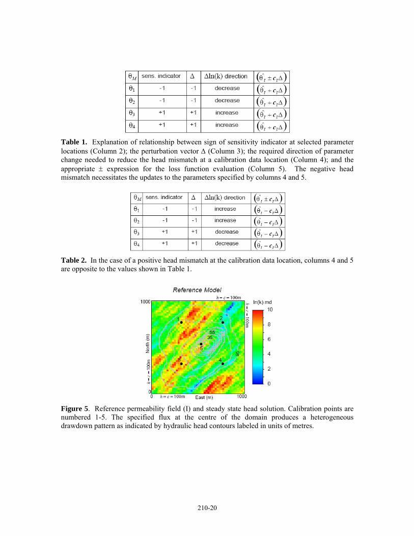
The first example consists of a 1000 x 1000 m square domain that is discretized as a 50 x 50 grid using a uniform cell size of 20 x 20 m. Reference field (I), taken as the “true field” (Figure 5), and all other permeability field realizations to be conditioned to the head data obtained on the reference field were generated by unconditional sequential Gaussian simulations using an anisotropic semivariogram with maximum continuity at an azimuth of 45 degrees. The

210-9

permeability histogram is lognormally distributed with a ln(k) mean and variance of 6.0 and 3.0, respectively.

Dirichlet boundaries are used with a hydraulic head of 100 m specified at each boundary cell. The flow equations were solved in steady state on reference field (I) in order to obtain the values for head at the five well locations to be used as the calibration data set (Figure 5). A constant withdrawal flux is specified at the center of the domain, plus four calibration points (C.P.’s) spaced equidistant from the “production well” (Figure 5) forming a five-spot pattern.

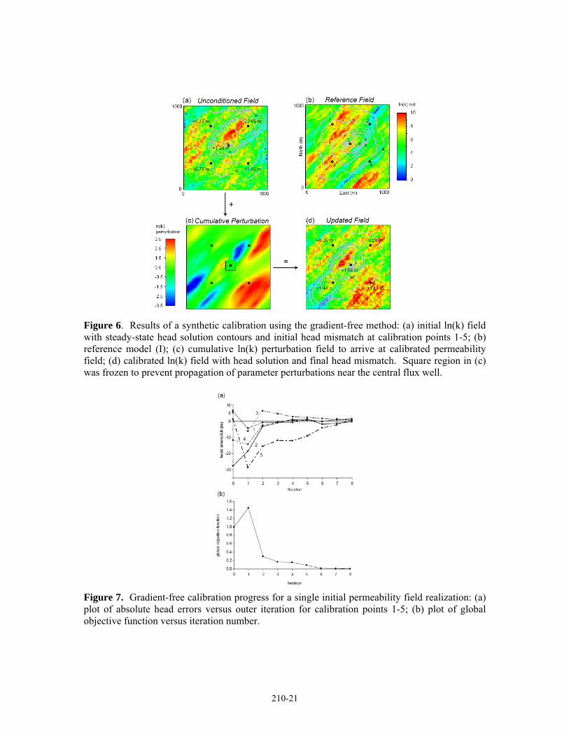
Conditioning a single realization

A single permeability realization was selected as an initial parameter field to be conditioned (Figure 6a). The initial field was selected from an ensemble of realizations such that the effective permeability in the near production well zone was similar to the reference field so there would be relatively small initial head mismatch at the flux well (Figure 6a). This was to ensure that near pumping-well effects did not dominate the calibration process in the first few iterations. In addition, during the calibration run, perturbations to the permeability field were frozen within a restricted zone around the flux well7 in order to prevent an artificial convergence of the calibration due to near-well effects. This would occur as a result of a large reduction in the effective permeability in the near-well zone, constricting the head response throughout the domain.

The initial head mismatch (Figures 6a, 7a) was reduced to 30% of the initial global calibration error at the second iteration (Figure 7b). The global objective function is the performance measure assessed at the outer calibration iterations (Figure 1) after solving for head on the updated permeability field. The global objective function at the lth outer iteration was specified as:

( )( )

( )( )1

2

θθ

F

hhF pnj

cj

oj

l

∑∈

−

= , (6)

After nine iterations the calibration converged to an objective function tolerance (Figure 7).

Conditioning an ensemble of realizations

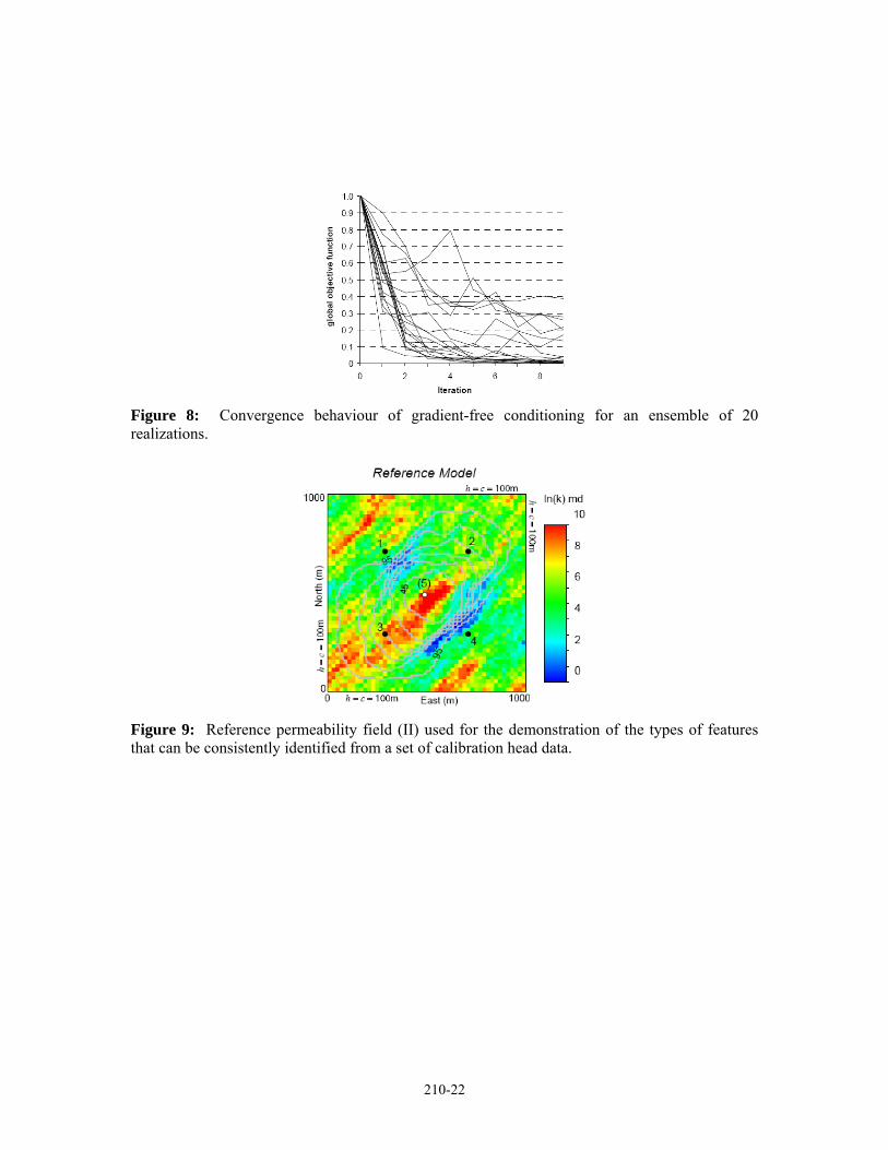
This example was rerun over an ensemble of 20 unconditional realizations. The constraint of having the correct effective permeability within the zone near the flux well is removed since there is no prior conditioning of the permeability fields (i.e., no conditioning to static data). The optimal permeability perturbations were also propagated freely over the domain, with no freezing of perturbations near the flux well.

More than half (13/20) of the calibration runs show a reduction of the global objective to a tight convergence (Figure 8). A few realizations are somewhat unstable and/or unable to converge to better than 40% of the initial calibration error. This indicates some sensitivity to the initial field, in particular, the effective permeability in the zone near the extraction well. The results indicate good performance of the algorithm by this somewhat unfair test. In practice the effective 7 Remark: If the pressure at the flux well was not included in the calibration data it was possible to get a good match at the other four points largely by reducing the effective permeability near the flux well. In this case, there would be a large negative pressure mismatch at the flux well. Both of these effects are undesirable.

210-10

permeability near production wells would be constrained, with the initial fields being conditioned to honour effective permeability from well-tests, for example. As an aside: if this was not the case, and a real study was to proceed as in this example, the success in achieving a satisfactory calibration to the head data would be a good plausibility measure. Those realizations for which a satisfactory calibration was not possible could be excluded from the final ensemble of conditioned realizations.

Identification of the reference field

It apparent from the shape of the drawdown on the potentiometric surface (Figure 6a,b,d) that calibration to only a few wells improves the identification of important features of the permeability field. In particular, the conduit of increased drawdown between the central flux well and C.P.3 is identified, and the overall shape of the head drawdown (Figure 6d) is much closer to the reference solution (Figure 6b) than the initial field (Figure 6a). Note that there is poor identification of the correct magnitudes of permeability structures defining features that effect the requisite pressure response to achieve calibration to the head data (Compare Figure 6b and d) . The specified flux at the centre of the domain does not provide sufficient flux data to arrive uniquely at correct effective permeability values which characterize important heterogeneities. The actual identification of geological features, based on a visual comparison between the reference field (Figure 6b) and the single calibrated field (Figure 6d), is fair. Indeed, we should not necessarily expect anything more from looking at a single realization conditioned to a set of pressure data.

The non-uniqueness of the solution to this inverse problem is well-known (Neuman, 1973; Carrera and Neuman, 1986b; Dietrich et al., 1989). Yet, there is potentially valuable information available from inverse conditioning to head data. The aim of conditioning is to reduce uncertainty in the flow response variables. In order to ensure a meaningful impact on global uncertainty through a reduction in parameter uncertainty, where the parameters are the values of permeability distributed throughout the model, key heterogeneity features that affect the flow response in the real system should be identified. Inverse conditioning to head data may or may not achieve this objective. An important question then, is: How much information can we expect from conditioning to a given configuration of head data?

From the sensitivity criteria listed previously, high-transmissivity conduits should be consistently identifiable where they are connected to a source or sink of fluid and intersected by streamlines passing through a calibration data location. High permeability features will not be reliably identified from head data in any other configuration. We can also expect to identify low permeability barriers along flowpaths coincident with any calibration head data location. The following examples illustrate these points.

Identification of flow barriers

The second example (Figure 9) considers a reference permeability field (reference field II) in a reservoir zone with good productivity near the production well and a high permeability conduit leading from near the production well to the SW boundary (Figure 9). Two of the observation wells (1 and 4) are completed in effectively poor reservoir quality zones because of the adjacent low permeability lenses. The flow solution is calculated on the reference field using the same model specifications as used in the previous example. Steady state heads are obtained from the four observation wells (1-4) for the calibration data set. The reason for the exclusion of the head at the production well from the calibration data set for this example is to isolate the conditioning effect of the calibration data that identify the low permeability lenses; namely, C.P. 1 and 4.

210-11

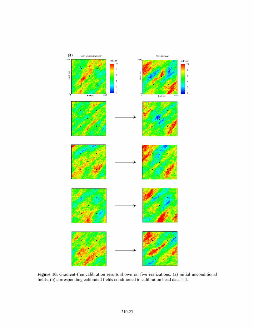
The gradient-free algorithm was applied to the same 20 initial unconditional realizations used in the previous example. Note, however, that that now a different reference field (II) is used as “truth” and to generate the calibration data. Compared to the initial realizations, the conditioned realizations quite consistently identify the two low permeability barriers between the central flux well and C.P.’s 1 and 4 (Figure 10)8.

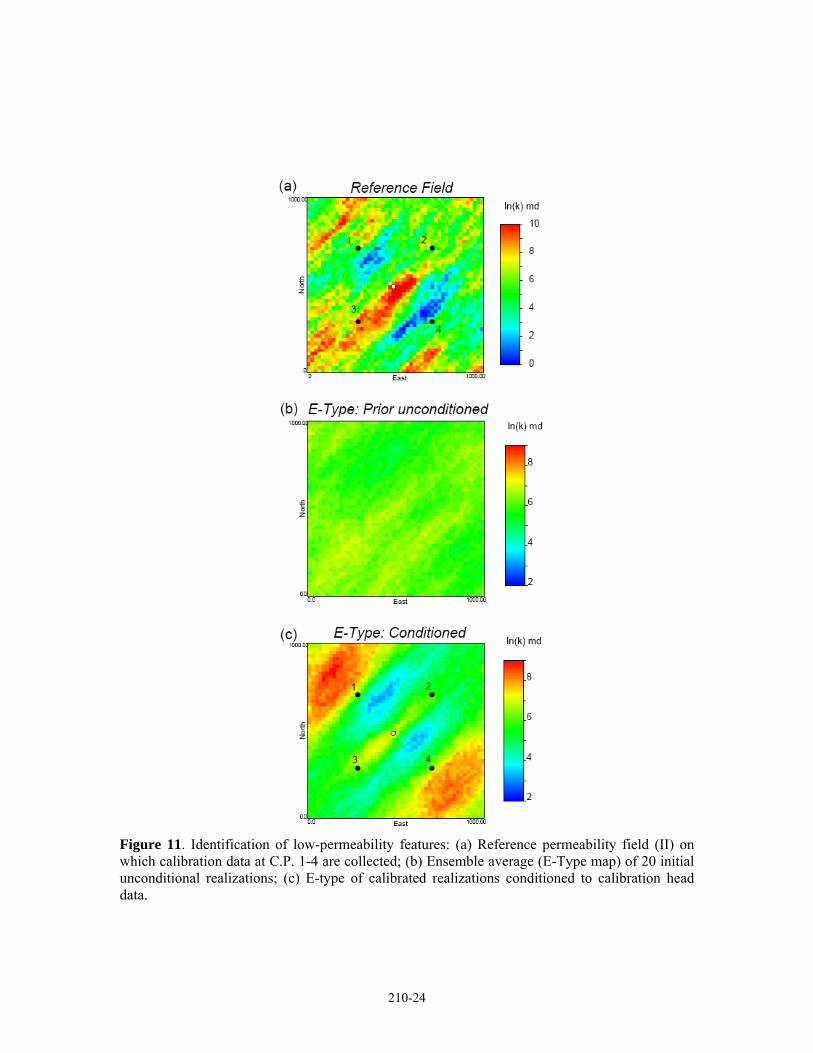
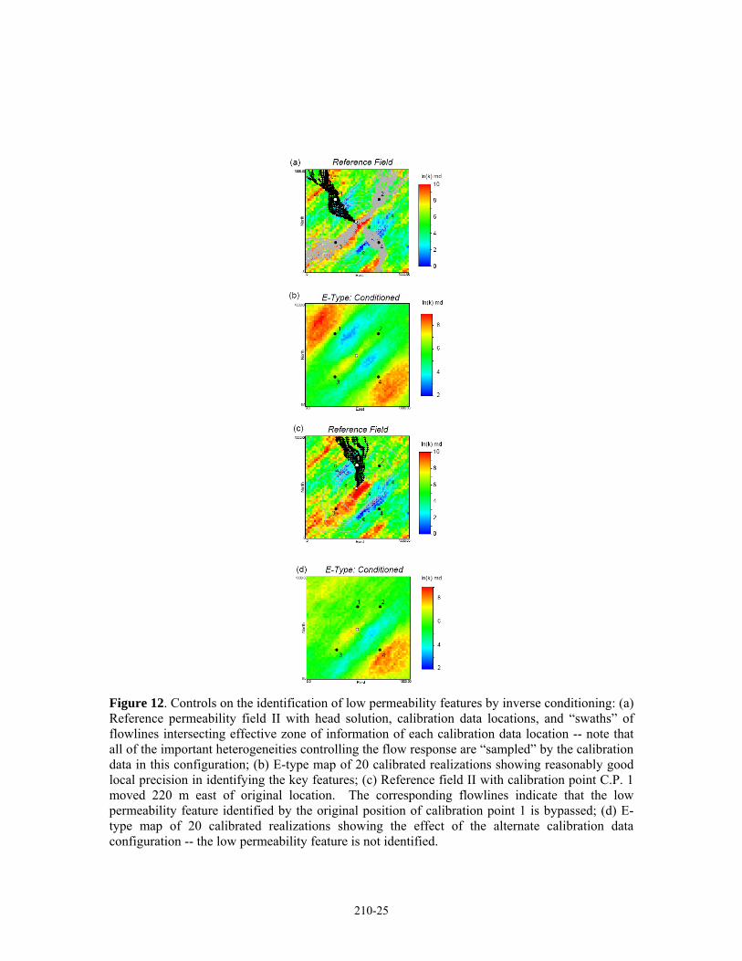
The ensemble average, or E-type map of the calibrated realizations9 (Figure 11) shows that good local accuracy can be expected in identifying low permeability barriers that are important in controlling the system response (i.e., the real system) as long as they are “sampled” by the calibration data. The swath of streamlines intersecting a calibration data location defines, to a first order, the effective zone of the model that the calibration data location informs. In order for a calibration point to inform a permeability barrier, that data location must be intersected by streamlines which also intersect the barrier (Figure 12a,b). Without this condition, it should not be possible to identify a permeability barrier, as is apparent by the effect of moving the location of C.P. 1 (Figure 12c,d); the low permeability lens in the NW quadrant of the domain is not identified. The basic criterion is that the anomaly in the head response that is produced by an important heterogeneity must be sampled by a calibration datum in order to identify the heterogeneity feature through an inverse approach. This is intuitive, but it is instructive to elucidate this point.

Identification of high-transmissivity conduits

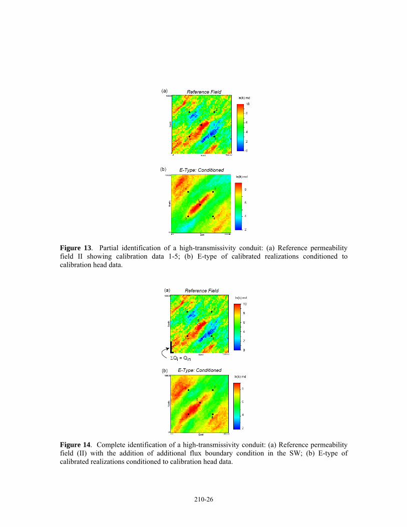
The same reference field (II) and flow model specifications are utilized in the following example, this time including the head at the central flux well as a calibration point (C.P. 5) in order to take advantage of the necessary flux constraint, as demonstrated next.

High-transmissivity conduits will be reliably identified between calibration head data and a source or sink in the domain. A source or sink represents valuable flux data, which constrain an otherwise non-unique head response. For example, the high permeability band in reference field II, located between the central well and C.P. 3 (Figure 9), is identified consistently in the calibrated fields (Figure 13). However, the connection between C.P. 3 and the SW boundary is not identified across all (or most) conditioned realizations (Figure 13). With only head specified at the boundary, there is no constraint on the flux passing through the zone where this conduit should be identified between C.P. 3 and the SW boundary. As is evident from the ensemble

8 Remark: Note how some features in the initial fields are completely changed, whereas others noticeably “seed” heterogeneities that result in a good calibration (Figure 10). This latter characteristic indicates that the algorithm preserves the initial field structure as much as possible. This is known as a “plausibility criterion” (Neuman, 1973) and it is an important aspect of regularizing the inverse problem (deMarsily, 2000). This is implicit to the SSC method in general; and it provides an example of how the SSC concept tackles the problem of obtaining a solution to the aquifer identification problem - as mentioned in the background section. 9 This is the best measure of the impact on the space of uncertainty by conditioning to the pressure data without actually assessing that space -- which is too large an undertaking to fit into the discussion. It suffices here to point out that if the most important heterogeneities are identified consistently in the realizations that summarize the spatial uncertainty model; then we have made the biggest impact that we could hope to have on the global uncertainty through the conditioning to pressure data.

210-12

average calibrated field, low permeability between the boundary and C.P. 3 is equally plausible (Figure 13b).

However, the specification of an additional boundary condition, an arbitrary flux at the SW boundary cells forming the “inlet” to the conduit (Figure 14a), results in a complete identification of the feature across all calibrated realizations (Figure 14b). In this case, the total inflow from the subset of boundary cells selected along the inlet to the conduit was made equal to the outflow at the well. From a practical modeling perspective, this is an inappropriate choice of boundary conditions for this system which has been assumed to have open boundaries, since the rest of the domain boundary now contributes a negligible amount of fluid to the production well; but it serves to illustrate the point. If the model were reduced to a “quarter five spot”, considering only the SW corner of the domain, and replacing the corner flux boundary by an injection well with a comparably high injection rate to the production rate at the producer, a high-transmissivity conduit between the injector and the producer would be consistently identified (e.g., Wen et al., 2005). The constraint to the solution set provided by the flux data coupled with head data which sample the anomaly produced by a high transmissivity feature uniquely identifies the heterogeneity.

Technological contribution

The key simplification that leads to the gradient-free approach — a complete yet fast assessment of parameter sensitivity — eliminates the need for specialized numerical procedures used to calculate sensitivity coefficients. This has been an area of extensive research for decades (e.g., Dogru and Seinfeld, 1981; Carrera et al., 1990; Oliver, 1994, Chu et al., 1995, Carrera et al., 1997; Landa et al., 1997). The rules-based method for sensitivity prediction that is at the heart of the gradient-free approach provides the modeler with a complete vector of sensitivity for each calibration location in the model (e.g., Figure 2e).

Obtaining the sensitivity indicator matrix permits a very effective parameterization of the optimization (Figure 4). In general, it is advantageous to have ready access to a complete assessment of sensitivity prior to approaching a model calibration. The ever-popular manual trial-and-error approach would benefit from a quick assessment of sensitivity for the entire model. A quick look at “sensitivity maps” (e.g., Figure 2e) at various iterations during a calibration procedure would offer the modeler insights into the calibration process that are not otherwise available.

With respect to savings in CPU time, it would be a major endeavor, that is beyond the scope of this study, to compare different methods given the number of variables involved, and the plethora of highly-specialized research codes. However, it is apparent that the elimination of the calculation of the Jacobian matrix, yet still utilizing sufficiently detailed sensitivity information in its place, is a major advantage in terms of computational efficiency over other sensitivity-based methods, with the possible exception of the Adjoint-state method10 (Medina and Carrera, 2003).

10 Even the clever concept of master points in SSC, which, for a small number of master points is on-par with the gradient-free method in efficiency, is at a disadvantage for two reasons: (1) CPU time is quite sensitive to the number of master points (this is not the case in the gradient-free approach), and (2) the parameterization offered by the original SSC sampling scheme is “blind” because of a lack of incorporation of prior sensitivity information (Figure 3), so if a small number of master points is used, you will generally not get a maximum amount of conditioning information from the inverse calibration to a pressure data set.

210-13

However, the method of Adjoint-states is a technically-involved procedure to implement, and the efficiency of the method depends on the number of observations (Medina and Carrera, 2003). Our gradient-free method is relatively insensitive to the number of observations.

The gradient-free approach could be considered a streamline or streamtube approach to inverse conditioning. Streamline-based history matching approaches have been proposed before (Wang and Kovscek, 2000; Caers et al., 2002; Wen et al., 2002). An important distinction that sets the gradient-free method apart from previous streamline-based methods for matching pressure data is that it is based on an understanding of the sensitivity process11 and an explicit account of sensitivities that can substitute directly for the calculation of the Jacobian. It is not only a bulk change along the streamlines/streamtubes that is proposed in order to obtain a match to the flow response (Wang and Kovscek, 2000; Caers et al., 2002); rather, spatially precise perturbations are made. This is because the selection of parameters to optimize is based on an assessment of the sensitivity structure of the field, of which streamlines are only one component. The method of Caers et al. (2002) also honours the geostatistical model of spatial uncertainty12, but because of the second point, will not guarantee local precision in identifying important heterogeneities. Caers et al. (2002) emphasize histogram and variogram reproduction though a Gauss-Markov iterative procedure; but the SSC approach, in general, will adequately reproduce these statistics without hard constraints, by preserving the structure of the prior model (Gomez-Hernandez et al., 1997; Xue and Datta-Gupta, 1997).

Seeding the perturbations from sensitive locations in the model, not simply a bulk change along a relevant streamtube, is critical to obtaining a good solution to the inversion problem; in particular, for preserving the prior permeability field structure, and more importantly, for identification of key heterogeneities affecting the flow response (Khan et al., in press). There is important information contained in pressure or head data which may allow spatially-accurate identification of permeability heterogeneity features if the calibration data sample them, and the approach of modifying effective permeability along streamlines cannot guarantee the identification of such features. Perhaps the best approach has been to combine a bulk streamline approach for rate and concentration data, and a traditional sensitivity method (i.e., SSC) to explicitly account for the pressure response (Wen et al., 2002). The simplified methodology presented in this paper solves the sensitivity problem for pressure such that an expensive numerical procedure is not needed to account for the pressure, thus simplifying the problem of integrating pressure, rate and concentration data, by a unified streamline approach that explicitly accounts for the information contained in the pressure data.

Conclusions

The gradient-free method is a relatively intuitive approach to calibrating the distributed parameter fields representing heterogeneous permeability in aquifer or reservoir models to head or pressure data. 11 It is only after a clear understanding of what controls the structure of sensitivity coefficients for pressure in reservoir models, that a streamtube approach is adopted. 12 They emphasize histogram and variogram reproduction though a Gauss-Markov iterative procedure; but the SSC approach, in general, will adequately reproduce these statistics without hard constraints. Moreover, the reproduction of these statistics is less critical than obtaining local precision in the calibrated realizations.

210-14

The method is based upon the procurement of a system of parameter sensitivities which replaces the need to calculate the Jacobian matrix. A rules-based approach for determining the required parameter sensitivity information is based upon: (1) delineation of flowpaths relevant to the calibration head data, (2) transforming the permeability field into a categorical variable in order to define relatively high-transmissivity and low-permeability geobodies, and (3) some connectivity measures identifying geobody connections to fluid sources or sinks in the model.

This results in identifying the sensitive grid cells to the response at the calibration data locations. The approximate direction of the gradient of the model response is determined from the sign on the sensitivity coefficients at selected parameters and the head mismatch at calibration locations. This information is used to construct the optimization problem for the calibration.

Parameter optimization is based on the deterministic gradient information inferred from the sign on the sensitivity coefficients and the head mismatch. The optimization algorithm uses an approximation of the gradient of the model response with respect to the parameters that is adapted from a proven gradient-free optimization technique (SPSA). Results from synthetic examples indicate good performance of the gradient-free algorithm under a reasonable suite of tests, including varying the reference and initial fields.

The method is partly based on a streamtube approach, whereby the conditioning effect of each calibration data point is seeded within the area covered by the locus of streamlines that intersects the calibration data location, with sensitive areas predicted by additional structural criteria coupled with the model specifications. From these insights, a framework is constructed to illustrate the effects of inverse conditioning to head data with respect to the information content that can be expected from the conditioning. Specifically: key heterogeneities which impact the flow response must be sampled by the calibration data. A calibration data point “samples” a heterogeneity feature when it occurs along a flowline that intersects the feature. By this approach, the permeability field can be adjusted within sensitive areas, seeding spatially precise perturbations to produce a head match at that calibration data location which results in an improvement in the local precision of the spatial uncertainty model from the conditioning process.

These general observations related to inverse conditioning to head data are not specific to the gradient-free approach. However, the constitutive elements of the gradient-free method lead to their clarification by adding a degree of transparency to the calibration process.

References

Caers, J., Krishnan, S., Wang, Y. and Kovscek, A.R., 2002. A Geostatistical Approach to Streamline-Based History Matching. Society of Petroleum Engineers Journal, 7(3): 250-266.

Capilla, J.E., Gomez-Hernandez, J.J. and Sahuquillo, A., 1997. Stochastic simulation of transmissivity fields conditional to both transmissivity and piezometric data; 2, Demonstration on a synthetic aquifer. Journal of Hydrology, 203(1-4): 175-188.

Capilla, J.E., Rodrigo, J. and Gomez-Hernandez, J.J., 1999. Simulation of Non-Gaussian Transmissivity Fields Honoring Piezometric Data and Integrating Soft and Secondary Information. Mathematical Geology, 31(7): 907-927.

Carrera, J. and Newman, S.P., 1986a. Estimation of aquifer parameters under transient and steady state conditions; 1, Maximum likelihood method incorporating prior information. Water Resources Research, 22(2): 199-210.

210-15

Carrera, J. and Newman, S.P., 1986b. Estimation of aquifer parameters under transient and steady state conditions; 2, Uniqueness, stability, and solution algorithms. Water Resources Research, 22(2): 211-227.

Carrera, J. and Newman, S.P., 1986c. Estimation of aquifer parameters under transient and steady state conditions; 3, Application to Synthetic and Field data. Water Resources Research, 22(2): 228-242.

Carrera, J., Navarrina, F., Viues, L., Heredia, J. and Medina, A., 1990. Computational aspects of the inverse problem. In: G. Gambolati, A. Rinaldo, C.A. Brebbia, W.G. Gray and F. Pinder George (Editors), Computational methods in subsurface hydrology. Comput. Mech. Publ., Southampton, United Kingdom, pp. 513-522.

Carrera, J., Medina, A., Axness, C. and Zimmerman, T., 1997. Formulations and computational issues of the inversion of random fields. In: G. Dagan and S.P. Neuman (Editors), Subsurface Flow and Transport: A Stochastic Approach. International Hydrology Series. Cambridge University Press, pp. 62-79.

Carrera, J., Alcolea, A., Medina, A., Hidalgo, J. and Slooten, L.J., 2005. Inverse problem in hydrogeology. Hydrogeology Journal, 13(1): 206-222.

Chu, L., Reynolds, A.C. and Oliver, D.S., 1995. Computation of sensitivity coefficients for conditioning the permeability field to well-test pressure data. In Situ, 19(2): 179-223.

de Marsily, G., Delhomme, J.P., Coudrain-Ribstein, A., Lavenue, A.M., (2000) Four Decades of Inverse Problems in Hydrogeology. Geophysical Society of America, Special Paper 348.

Dietrich, C.R., Newsam, G.N., Anderssen, R.S., Ghassemi, F. and Jakeman, A.J., 1989. A practical account of instabilities in identification problems in groundwater systems. BMR Journal of Australian Geology and Geophysics, 11: 273-284.

Dogru, A.H. and Seinfeld, J.H., 1981. Comparison of Sensitivity Coefficient Calculation Methods in Automatic History Matching. Society of Petroleum Engineers Journal: 551-557.

Emsellem, Y. and de Marsily, G., 1971. An automatic Solution for the inverse problem. Water Resources Research, 7(5): 1264-1283.

Gomez-Hernandez, J.J., Sahuquillo, A. and Capilla, J.E., 1997. Stochastic simulation of transmissivity fields conditional to both transmissivity and piezometric data; I, Theory. Journal of Hydrology, 203(1-4): 162-174.

Kitanidis, P.K. and Vomvoris, E.G., 1983. A geostatistical approach to the inverse problem in groundwater modeling (steady state) and one-dimensional simulations. Water Resources Research, 19(3): 677-690.

Landa, J.L. and Horne, R.N., 1997. A Procedure to Integrate Well Test Data, Reservoir Performance History and 4-D Seismic Information into a Reservoir Description, SPE Paper 38653 presented at SPE Annual Technical Conference and Exhibition. Society of Petroleum Engineers, San Antonio, TX, pp. 177-192.

Medina, A. and Carrera, J., 2003. Geostatistical inversion of coupled problems: dealing with computational burden and different types of data. Journal of Hydrology, 281(4): 251-264.

210-16

Neuman, S.P., 1973. Calibration of Distributed Parameter Groundwater Flow Models Viewed as a Multiple-Objective Decision Process under Uncertainty. Water Resources Research, 9(4): 1006-1021.

RamaRao, B.S., LaVenue, A.M., de Marsily, G., and Marietta, M.G., 1995. Pilot point methodology for automated calibration of an ensemble of conditionally simulated transmissivity fields; 1, Theory and computational experiments. Water Resources Research, 31(3): 475-493.

Sykes, J.F., Wilson, J.L. and Andrews, R.W., 1985. Sensitivity Analysis for Steady State Groundwater Flow Using Adjoint Operators. Water Resources Research, 21(3): 359-371.

Spall, J.C., 1992. Multivariate Stochastic Approximation Using a Simultaneous Perturbation Gradient Approximation. IEEE Transactions on Automatic Control, 37: 332-341.

Spall, J.C., 1998. Implementation of the Simultaneous Perturbation Algorithm for Stochastic Optimization. IEEE Transactions on Aerospace and Electronic Systems, 34: 817-823.

Spall, J.C., 2003. Simultaneous Perturbation Stochastic Approximation, Introduction to Stochastic Search and Optimization: Estimation, Simulation, and Control. Wiley-Interscience series in discrete mathematics. John Wiley and Sons, Inc., Hoboken, New Jersey, pp. 177-230.

Wang, Y. and Kovscek, A., 2000. A Streamline Approach for History-Matching Production Data, SPE Paper 59370 presented at SPE/DOE Improved Oil Recovery Symposium, Tulsa, Oklahoma, pp. 1-8.

Wen, X.H., Capilla, J.E., Deutsch, C.V., Gomez-Hernandez, J.J. and Cullick, A.S., 1999. A program to create permeability fields that honor single-phase flow rate and pressure data. Computers & Geosciences, 25: 217-230.

Wen, X.H., Deutsch, C.V. and Cullick, A.S., 2002. Construction of geostatistical aquifer models integrating dynamic flow and tracer data using inverse technique. Journal of Hydrology, 255: 151-168.

Wen, X.H., Deutsch, C.V., Cullick, A.S. and Reza, Z.A., 2005. Integration of Production Data in Generating Reservoir Models. Centre for Computational Geostatistics Monograph Series, 1. Centre for Computational Geostatistics, pp. 85-93.

Xue, G. and Datta-Gupta, A., 1997. Structure Preserving Inversion: An Efficient Approach to Conditioning Stochastic Reservoir Models to Dynamic Data, SPE Paper 38727 presented at 1997 SPE Annual Technical Conference and Exhibition. SPE, San Antonio, TX, pp. 101-113.

210-17

Figure 1. General flow chart depicting the Sequential Self Calibration (SSC) algorithm with gradient-free method (boxed) incorporated.

210-18

Figure 2. The process of obtaining approximate sensitivity indicators of head response at four calibration locations to the permeability field. (a) Permeability field structure, locations of calibration data, and contours of head due to pumping well at centre of model; (b) histogram of lognormal transform of permeability with ln(k) cutoff of 0.0 used to define two classes of geobodies; (c) binary geobody classification defining relatively transmissive and flow-retarding geobodies; (d) streamline tracks intersecting the four calibration data locations; (e) sensitivity indicator maps corresponding to the vector of sensitivity for each calibration location. Numbered geobodies are referenced in text.

210-19

Figure 3. Comparison of the parameterization scheme preceding the optimization routine in (a) the original SSC method, which uses a random stratified sampling scheme; and (b) the gradient-free approach which uses the prior prediction of sensitivities to constrain the random drawing of a parameter subset (stars) to sensitive areas of the model given a specific configuration of calibration data (circles).

Figure 4. An example of the parameterization of the optimization to reduce the head mismatch at a specific calibration location. (a) The initial head solution and the head mismatch at a calibration data location; (b) the vector of sensitivity indicators and a selected parameter subset {θ} corresponding to sensitive grid cells to the response calibration data location.

210-20

Table 1. Explanation of relationship between sign of sensitivity indicator at selected parameter locations (Column 2); the perturbation vector Δ (Column 3); the required direction of parameter change needed to reduce the head mismatch at a calibration data location (Column 4); and the appropriate ± expression for the loss function evaluation (Column 5). The negative head mismatch necessitates the updates to the parameters specified by columns 4 and 5.

Table 2. In the case of a positive head mismatch at the calibration data location, columns 4 and 5 are opposite to the values shown in Table 1.

Figure 5. Reference permeability field (I) and steady state head solution. Calibration points are numbered 1-5. The specified flux at the centre of the domain produces a heterogeneous drawdown pattern as indicated by hydraulic head contours labeled in units of metres.

210-21

Figure 6. Results of a synthetic calibration using the gradient-free method: (a) initial ln(k) field with steady-state head solution contours and initial head mismatch at calibration points 1-5; (b) reference model (I); (c) cumulative ln(k) perturbation field to arrive at calibrated permeability field; (d) calibrated ln(k) field with head solution and final head mismatch. Square region in (c) was frozen to prevent propagation of parameter perturbations near the central flux well.

Figure 7. Gradient-free calibration progress for a single initial permeability field realization: (a) plot of absolute head errors versus outer iteration for calibration points 1-5; (b) plot of global objective function versus iteration number.

210-22

Figure 8: Convergence behaviour of gradient-free conditioning for an ensemble of 20 realizations.

Figure 9: Reference permeability field (II) used for the demonstration of the types of features that can be consistently identified from a set of calibration head data.

210-23

Figure 10. Gradient-free calibration results shown on five realizations: (a) initial unconditional fields; (b) corresponding calibrated fields conditioned to calibration head data 1-4.

210-24

Figure 11. Identification of low-permeability features: (a) Reference permeability field (II) on which calibration data at C.P. 1-4 are collected; (b) Ensemble average (E-Type map) of 20 initial unconditional realizations; (c) E-type of calibrated realizations conditioned to calibration head data.

210-25

Figure 12. Controls on the identification of low permeability features by inverse conditioning: (a) Reference permeability field II with head solution, calibration data locations, and “swaths” of flowlines intersecting effective zone of information of each calibration data location -- note that all of the important heterogeneities controlling the flow response are “sampled” by the calibration data in this configuration; (b) E-type map of 20 calibrated realizations showing reasonably good local precision in identifying the key features; (c) Reference field II with calibration point C.P. 1 moved 220 m east of original location. The corresponding flowlines indicate that the low permeability feature identified by the original position of calibration point 1 is bypassed; (d) E-type map of 20 calibrated realizations showing the effect of the alternate calibration data configuration -- the low permeability feature is not identified.

210-26

Figure 13. Partial identification of a high-transmissivity conduit: (a) Reference permeability field II showing calibration data 1-5; (b) E-type of calibrated realizations conditioned to calibration head data.

Figure 14. Complete identification of a high-transmissivity conduit: (a) Reference permeability field (II) with the addition of additional flux boundary condition in the SW; (b) E-type of calibrated realizations conditioned to calibration head data.