A GPU accelerated algorithm for 3D Delaunay triangulationtants/gdel3d_files/gDel3D.pdf ·...
8
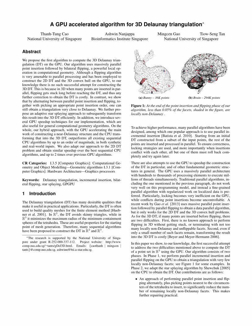
A GPU accelerated algorithm for 3D Delaunay triangulation * Thanh-Tung Cao National University of Singapore Ashwin Nanjappa Bioinformatics Institute Singapore Mingcen Gao Tiow-Seng Tan National University of Singapore Abstract We propose the first algorithm to compute the 3D Delaunay trian- gulation (DT) on the GPU. Our algorithm uses massively parallel point insertion followed by bilateral flipping, a powerful local op- eration in computational geometry. Although a flipping algorithm is very amenable to parallel processing and has been employed to construct the 2D DT and the 3D convex hull on the GPU, to our knowledge there is no such successful attempt for constructing the 3D DT. This is because in 3D when many points are inserted in par- allel, flipping gets stuck long before reaching the DT, and thus any further correction to obtain the DT is costly. In contrast, we show that by alternating between parallel point insertion and flipping, to- gether with picking an appropriate point insertion order, one can still obtain a triangulation very close to Delaunay. We further pro- pose an adaptive star splaying approach to subsequently transform this result into the 3D DT efficiently. In addition, we introduce sev- eral GPU speedup techniques for our implementation, which are also useful for general computational geometry algorithms. On the whole, our hybrid approach, with the GPU accelerating the main work of constructing a near-Delaunay structure and the CPU trans- forming that into the 3D DT, outperforms all existing sequential CPU algorithms by up to an order of magnitude, in both synthetic and real-world inputs. We also adapt our approach to the 2D DT problem and obtain similar speedup over the best sequential CPU algorithms, and up to 2 times over previous GPU algorithms. CR Categories: I.3.5 [Computer Graphics]: Computational Ge- ometry and Object Modelling—Geometric algorithms I.3.1 [Com- puter Graphics]: Hardware Architecture—Graphics processors Keywords: Delaunay triangulation, incremental insertion, bilat- eral flipping, star splaying, GPGPU 1 Introduction The Delaunay triangulation (DT) has many desirable qualities that make it useful in practical applications. Particularly, the DT is often used to build quality meshes for the finite element method [Hueb- ner et al. 2001]. In R 2 , the DT avoids skinny triangles, while in R 3 it minimizes the maximum radius of the minimum containment spheres of the tetrahedra. These are useful properties for the starting point of mesh generation. Therefore, many sequential algorithms have been proposed to construct the DT in R 2 and R 3 . * The research is supported by the National University of Singa- pore under grant R-252-000-337-112. Project website: http://www. comp.nus.edu.sg/ ∼ tants/gDel3D.html. Emails: {caothanh | mingcen | tants}@comp.nus.edu.sg, [email protected]. (a) Bunny – 36K points (b) Brain – 294K points Figure 1: At the end of the point insertion and flipping phase of our algorithm, less than 0.05% of the facets, shaded in the figure, are locally non-Delaunay . To achieve higher performance, many parallel algorithms have been designed, among which one popular approach is to use parallel in- cremental insertion [Batista et al. 2010]. Starting from an initial DT constructed from a subset of the input points, the rest of the points are inserted and processed in parallel. To ensure correctness, locking strategies are used, and more importantly when insertions conflict with each other, all but one of them must roll back com- pletely and try again later. There are also attempts to use the GPU to speedup the construction of the DT in particular, and of other fundamental geometric struc- tures in general. The GPU uses a massively parallel architecture with hundreds to thousands of processing elements to execute mil- lions of threads simultaneously. Traditional parallel algorithms, in- cluding the one mentioned in the previous paragraph, do not work very well on this programming model, and instead a fine-grained parallel algorithm with regularized work on localized data is pre- ferred. Particularly, locking becomes very inefficient on the GPU, while conflicts during point insertions become uncontrollable. A recent work by Gao et al. [2013] uses massive parallel point inser- tion followed by parallel flipping to obtain a data parallel algorithm, but it only works for the 2D DT and the 3D convex hull problems. As for the 3D DT, if many points are inserted before flipping, there are two difficulties. First, there is no known approach to perform flipping in 3D without getting stuck, or terminating with not too many locally non-Delaunay and unflippable facets. Second, even if only a small number of such facets remain, transforming the result into the 3D DT is costly [Beyer and Meyer-Hermann 2006]. In this paper we show, to our knowledge, the first successful attempt to address the two difficulties mentioned above to compute the DT of a point set in R 3 using the GPU. Our algorithm consists of two phases. In Phase 1, we perform parallel incremental insertion and parallel flipping on the GPU to obtain a triangulation with very few locally non-Delaunay facets; see Figure 1 for some examples. In Phase 2, we adapt the star splaying algorithm by Shewchuk [2005] on the CPU to obtain the DT. Our contributions are as follows: • An approach of performing parallel point insertion and flip- ping alternately, plus picking points nearest to the circumcen- ters of the tetrahedra to insert, to significantly reduce the num- ber of remaining locally non-Delaunay facets. This makes further repairing practical.
Transcript of A GPU accelerated algorithm for 3D Delaunay triangulationtants/gdel3d_files/gDel3D.pdf ·...
A GPU accelerated algorithm for 3D Delaunay triangulation∗
Thanh-Tung CaoNational University of Singapore
Ashwin NanjappaBioinformatics Institute Singapore
Mingcen Gao Tiow-Seng TanNational University of Singapore
Abstract
We propose the first algorithm to compute the 3D Delaunay trian-gulation (DT) on the GPU. Our algorithm uses massively parallelpoint insertion followed by bilateral flipping, a powerful local op-eration in computational geometry. Although a flipping algorithmis very amenable to parallel processing and has been employed toconstruct the 2D DT and the 3D convex hull on the GPU, to ourknowledge there is no such successful attempt for constructing the3D DT. This is because in 3D when many points are inserted in par-allel, flipping gets stuck long before reaching the DT, and thus anyfurther correction to obtain the DT is costly. In contrast, we showthat by alternating between parallel point insertion and flipping, to-gether with picking an appropriate point insertion order, one canstill obtain a triangulation very close to Delaunay. We further pro-pose an adaptive star splaying approach to subsequently transformthis result into the 3D DT efficiently. In addition, we introduce sev-eral GPU speedup techniques for our implementation, which arealso useful for general computational geometry algorithms. On thewhole, our hybrid approach, with the GPU accelerating the mainwork of constructing a near-Delaunay structure and the CPU trans-forming that into the 3D DT, outperforms all existing sequentialCPU algorithms by up to an order of magnitude, in both syntheticand real-world inputs. We also adapt our approach to the 2D DTproblem and obtain similar speedup over the best sequential CPUalgorithms, and up to 2 times over previous GPU algorithms.
CR Categories: I.3.5 [Computer Graphics]: Computational Ge-ometry and Object Modelling—Geometric algorithms I.3.1 [Com-puter Graphics]: Hardware Architecture—Graphics processors
Keywords: Delaunay triangulation, incremental insertion, bilat-eral flipping, star splaying, GPGPU
1 Introduction
The Delaunay triangulation (DT) has many desirable qualities thatmake it useful in practical applications. Particularly, the DT is oftenused to build quality meshes for the finite element method [Hueb-ner et al. 2001]. In R2, the DT avoids skinny triangles, while inR3 it minimizes the maximum radius of the minimum containmentspheres of the tetrahedra. These are useful properties for the startingpoint of mesh generation. Therefore, many sequential algorithmshave been proposed to construct the DT in R2 and R3.
∗The research is supported by the National University of Singa-pore under grant R-252-000-337-112. Project website: http://www.comp.nus.edu.sg/∼tants/gDel3D.html. Emails: {caothanh | mingcen |tants}@comp.nus.edu.sg, [email protected].
(a) Bunny – 36K points
(b) Brain – 294K points
Figure 1: At the end of the point insertion and flipping phase of ouralgorithm, less than 0.05% of the facets, shaded in the figure, arelocally non-Delaunay .
To achieve higher performance, many parallel algorithms have beendesigned, among which one popular approach is to use parallel in-cremental insertion [Batista et al. 2010]. Starting from an initialDT constructed from a subset of the input points, the rest of thepoints are inserted and processed in parallel. To ensure correctness,locking strategies are used, and more importantly when insertionsconflict with each other, all but one of them must roll back com-pletely and try again later.
There are also attempts to use the GPU to speedup the constructionof the DT in particular, and of other fundamental geometric struc-tures in general. The GPU uses a massively parallel architecturewith hundreds to thousands of processing elements to execute mil-lions of threads simultaneously. Traditional parallel algorithms, in-cluding the one mentioned in the previous paragraph, do not workvery well on this programming model, and instead a fine-grainedparallel algorithm with regularized work on localized data is pre-ferred. Particularly, locking becomes very inefficient on the GPU,while conflicts during point insertions become uncontrollable. Arecent work by Gao et al. [2013] uses massive parallel point inser-tion followed by parallel flipping to obtain a data parallel algorithm,but it only works for the 2D DT and the 3D convex hull problems.As for the 3D DT, if many points are inserted before flipping, thereare two difficulties. First, there is no known approach to performflipping in 3D without getting stuck, or terminating with not toomany locally non-Delaunay and unflippable facets. Second, even ifonly a small number of such facets remain, transforming the resultinto the 3D DT is costly [Beyer and Meyer-Hermann 2006].
In this paper we show, to our knowledge, the first successful attemptto address the two difficulties mentioned above to compute the DTof a point set in R3 using the GPU. Our algorithm consists of twophases. In Phase 1, we perform parallel incremental insertion andparallel flipping on the GPU to obtain a triangulation with very fewlocally non-Delaunay facets; see Figure 1 for some examples. InPhase 2, we adapt the star splaying algorithm by Shewchuk [2005]on the CPU to obtain the DT. Our contributions are as follows:
• An approach of performing parallel point insertion and flip-ping alternately, plus picking points nearest to the circumcen-ters of the tetrahedra to insert, to significantly reduce the num-ber of remaining locally non-Delaunay facets. This makesfurther repairing practical.
Tants
Typewritten Text
Tants
Typewritten Text
Tants
Typewritten Text
ACM SIGGRAPH Symposium on Interactive 3D Graphics and Games (2014): 47-54. New York: ACM.
• An adaptive approach for the star splaying algorithm so thatthe work performed is proportional to the amount of modifi-cations needed in getting to the DT.
• Several key GPU techniques, such as handling exact compu-tation and point location, to accelerate our implementation.These are also of independent interest to implementing othercomputational geometry algorithms on the GPU.
The implementation of our hybrid GPU-CPU algorithm outper-forms all existing 3D DT implementations on the CPU by up toan order of magnitude, for both synthetic and real-world data. Byadapting the approach of Phase 1 to solve the 2D DT problem onthe GPU, we also observe up to an order of magnitude speedup overexisting 2D DT implementations on the CPU, and up to 2–5 timesspeedup over other GPU implementations.
In the following section, we first introduce some basic terminolo-gies and a few related works. Section 3 and Section 4 detail ouralgorithm and some implementation techniques. In Section 5 wepresent the experimental analysis of our implementation, beforeconcluding the paper with the limitations and possible future worksin Section 6.
2 Preliminaries
In R3, given a set S of points, the Delaunay triangulation (DT)D(S) of S is a triangulation of S such that the circumsphere of anytetrahedron in D(S) does not contain any other point in S. Givena triangulation T of S, a triangle, or facet, f ∈ T is said to belocally Delaunay if and only if it has only one link vertex, or eachcircumsphere of the tetrahedron formed by f and one of its linkvertices does not contain the other vertex. Otherwise, the facet islocally non-Delaunay. If every facet of T is locally Delaunay, thenT ≡ D(S) [Lawson 1987].
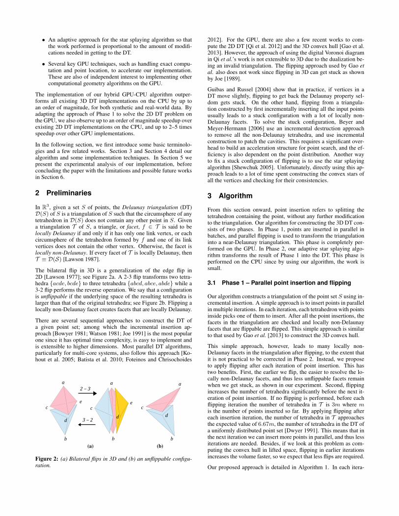
The bilateral flip in 3D is a generalization of the edge flip in2D [Lawson 1977]; see Figure 2a. A 2-3 flip transforms two tetra-hedra {acde, bcde} to three tetrahedra {abcd, abce, abde} while a3-2 flip performs the reverse operation. We say that a configurationis unflippable if the underlying space of the resulting tetrahedra islarger than that of the original tetrahedra; see Figure 2b. Flipping alocally non-Delaunay facet creates facets that are locally Delaunay.
There are several sequential approaches to construct the DT ofa given point set; among which the incremental insertion ap-proach [Bowyer 1981; Watson 1981; Joe 1991] is the most popularone since it has optimal time complexity, is easy to implement andis extensible to higher dimensions. Most parallel DT algorithms,particularly for multi-core systems, also follow this approach [Ko-hout et al. 2005; Batista et al. 2010; Foteinos and Chrisochoides
a
ce
d
b
a
ce
b
2 ‒ 3
3 ‒ 2d
(a)
a
c
b
d
(b)
Figure 2: (a) Bilateral flips in 3D and (b) an unflippable configu-ration.
2012]. For the GPU, there are also a few recent works to com-pute the 2D DT [Qi et al. 2012] and the 3D convex hull [Gao et al.2013]. However, the approach of using the digital Voronoi diagramin Qi et al.’s work is not extensible to 3D due to the dualization be-ing an invalid triangulation. The flipping approach used by Gao etal. also does not work since flipping in 3D can get stuck as shownby Joe [1989].
Guibas and Russel [2004] show that in practice, if vertices in aDT move slightly, flipping to get back the Delaunay property sel-dom gets stuck. On the other hand, flipping from a triangula-tion constructed by first incrementally inserting all the input pointsusually leads to a stuck configuration with a lot of locally non-Delaunay facets. To solve the stuck configuration, Beyer andMeyer-Hermann [2006] use an incremental destruction approachto remove all the non-Delaunay tetrahedra, and use incrementalconstruction to patch the cavities. This requires a significant over-head to build an acceleration structure for point search, and the ef-ficiency is also dependent on the point distribution. Another wayto fix a stuck configuration of flipping is to use the star splayingalgorithm [Shewchuk 2005]. Unfortunately, directly using this ap-proach leads to a lot of time spent constructing the convex stars ofall the vertices and checking for their consistencies.
3 Algorithm
From this section onward, point insertion refers to splitting thetetrahedron containing the point, without any further modificationto the triangulation. Our algorithm for constructing the 3D DT con-sists of two phases. In Phase 1, points are inserted in parallel inbatches, and parallel flipping is used to transform the triangulationinto a near-Delaunay triangulation. This phase is completely per-formed on the GPU. In Phase 2, our adaptive star splaying algo-rithm transforms the result of Phase 1 into the DT. This phase isperformed on the CPU since by using our algorithm, the work issmall.
3.1 Phase 1 – Parallel point insertion and flipping
Our algorithm constructs a triangulation of the point set S using in-cremental insertion. A simple approach is to insert points in parallelin multiple iterations. In each iteration, each tetrahedron with pointsinside picks one of them to insert. After all the point insertions, thefacets in the triangulation are checked and locally non-Delaunayfacets that are flippable are flipped. This simple approach is similarto that used by Gao et al. [2013] to construct the 3D convex hull.
This simple approach, however, leads to many locally non-Delaunay facets in the triangulation after flipping, to the extent thatit is not practical to be corrected in Phase 2. Instead, we proposeto apply flipping after each iteration of point insertion. This hastwo benefits. First, the earlier we flip, the easier to resolve the lo-cally non-Delaunay facets, and thus less unflippable facets remainwhen we get stuck, as shown in our experiment. Second, flippingincreases the number of tetrahedra significantly before the next it-eration of point insertion. If no flipping is performed, before eachflipping iteration the number of tetrahedra in T is 3m where mis the number of points inserted so far. By applying flipping aftereach insertion iteration, the number of tetrahedra in T approachesthe expected value of 6.67m, the number of tetrahedra in the DT ofa uniformly distributed point set [Dwyer 1991]. This means that inthe next iteration we can insert more points in parallel, and thus lessiterations are needed. Besides, if we look at this problem as com-puting the convex hull in lifted space, flipping in earlier iterationsincreases the volume faster, so we expect that less flips are required.
Our proposed approach is detailed in Algorithm 1. In each itera-
Algorithm 1: Incremental insertion and flipping.Data: A point set SResult: D(S)
1 initialize T with a large enough tetrahedron t2 for each p ∈ S do in parallel location[p]← t3 while ¬Empty(S) do4 for each p ∈ S do in parallel insert[location[p]]← p5 for each t ∈ T with insert[t] 6= null do in parallel6 split t using insert[t] and remove insert[t] from S7 label all new facets to be checked8 while there are facets to be checked do9 for each facet f that needs to be checked do in parallel
10 if f is locally non-Delaunay and flippable then11 flip f12 label all updated facets to be checked13 end14 update the location of points in S15 end16 return T
tion, we first pick for each tetrahedron a point inside it to insert, ifany (line 4). Then we split the tetrahedron and update its neighbors(line 5–7). We also label the new facets so that they are checkedin the subsequent flipping. The flipping is performed right after abatch of points is inserted (line 8–13). We repeatedly check thefacets in T to find those locally non-Delaunay facets that are flip-pable, flip them, and update the neighboring information. Finally,we update the location of the points that are left in S if its old lo-cation was split (line 14), to prepare for the next round of pointinsertion.
In each iteration, when there are tetrahedra containing multiplepoints, we need to pick one of them to insert. Typical optionsare choosing randomly, or choosing one near the centroid of thetetrahedron. Instead, we propose to insert the point that is nearestto the circumcenter of that tetrahedron. The motivation is as fol-lows. Constructing the DT is equivalent to constructing the lowerhull when the input points are lifted to R4, i.e. the point (x, y, z) istransformed into the point (x, y, z, x2+y2+z2). Inserting the pointnearest to the circumcenter of the tetrahedron is the same as insert-ing the point furthest to the lifted face. In doing so, the volume ofthe hull grows the most and is closer to that of the convex hull, thusthe number of flipping in the next phase can be reduced. Anotherreason is that the point nearest to the circumcenter is also the fur-thest from the vertices of the tetrahedron, i.e. the minimum distanceis maximum. Therefore, the facets created during the insertion areof better quality and thus it is also easier for the subsequent flipping.We show in our experiment that by applying this heuristic, not onlydoes the number of flips decrease, but the number of locally non-Delaunay facets at the end of Phase 1 also decreases, thus reducingthe effort needed in Phase 2.
The result of this phase is a triangulation that is very close to the DT.There are still facets that are not locally Delaunay but are all unflip-pable. Using our strategy, this number is usually very small. Fig-ure 1 shows the locally non-Delaunay facets at the end of Phase 1during the DT construction of two 3D models.
3.2 Phase 2 – Adaptive star splaying
The star splaying algorithm used in this section to transform theresult of Phase 1 into the DT is adaptive, and is done sequentiallyon the CPU. As we show in our experiment, the work needed hereis small and thus does not affect the performance of our algorithm.
locally non-Delaunay, unflippable
stars arenon-convex
stars areirrelevant
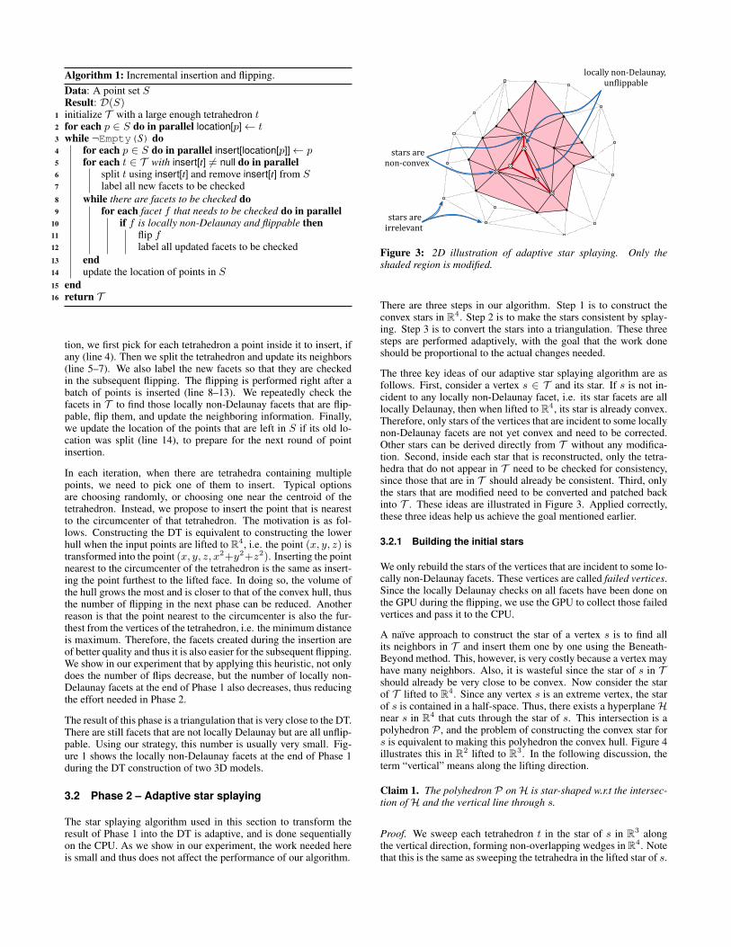
Figure 3: 2D illustration of adaptive star splaying. Only theshaded region is modified.
There are three steps in our algorithm. Step 1 is to construct theconvex stars in R4. Step 2 is to make the stars consistent by splay-ing. Step 3 is to convert the stars into a triangulation. These threesteps are performed adaptively, with the goal that the work doneshould be proportional to the actual changes needed.
The three key ideas of our adaptive star splaying algorithm are asfollows. First, consider a vertex s ∈ T and its star. If s is not in-cident to any locally non-Delaunay facet, i.e. its star facets are alllocally Delaunay, then when lifted to R4, its star is already convex.Therefore, only stars of the vertices that are incident to some locallynon-Delaunay facets are not yet convex and need to be corrected.Other stars can be derived directly from T without any modifica-tion. Second, inside each star that is reconstructed, only the tetra-hedra that do not appear in T need to be checked for consistency,since those that are in T should already be consistent. Third, onlythe stars that are modified need to be converted and patched backinto T . These ideas are illustrated in Figure 3. Applied correctly,these three ideas help us achieve the goal mentioned earlier.
3.2.1 Building the initial stars
We only rebuild the stars of the vertices that are incident to some lo-cally non-Delaunay facets. These vertices are called failed vertices.Since the locally Delaunay checks on all facets have been done onthe GPU during the flipping, we use the GPU to collect those failedvertices and pass it to the CPU.
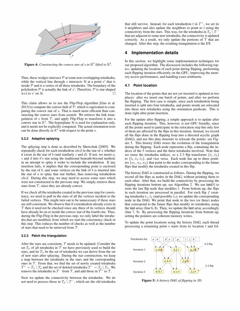
A naıve approach to construct the star of a vertex s is to find allits neighbors in T and insert them one by one using the Beneath-Beyond method. This, however, is very costly because a vertex mayhave many neighbors. Also, it is wasteful since the star of s in Tshould already be very close to be convex. Now consider the starof T lifted to R4. Since any vertex s is an extreme vertex, the starof s is contained in a half-space. Thus, there exists a hyperplaneHnear s in R4 that cuts through the star of s. This intersection is apolyhedron P , and the problem of constructing the convex star fors is equivalent to making this polyhedron the convex hull. Figure 4illustrates this in R2 lifted to R3. In the following discussion, theterm “vertical” means along the lifting direction.
Claim 1. The polyhedron P onH is star-shaped w.r.t the intersec-tion ofH and the vertical line through s.
Proof. We sweep each tetrahedron t in the star of s in R3 alongthe vertical direction, forming non-overlapping wedges in R4. Notethat this is the same as sweeping the tetrahedra in the lifted star of s.
H
s
P
s'
Figure 4: Constructing the convex star of s in R2 lifted to R3.
Thus, these wedges intersectP at some non-overlapping tetrahedra,while the vertical line through s intersects H at a point s′ that isinside P and is a vertex of all these tetrahedra. The boundary of thepolyhedron P is actually the link of s′. Therefore, P is star-shapedw.r.t to s′ onH.
This claim allows us to use the Flip-Flop algorithm [Gao et al.2013] to compute the convex hull of P , which is equivalent to com-puting the convex star of s. That is much more efficient than con-structing the convex stars from scratch. We retrieve the link trian-gulation of s from T , and apply Flip-Flop to transform it into aconvex star in R4. The hyperplane H is used for explanation only,and it needs not be explicitly computed. The actual orientation testscan be done directly in R4 with respect to the point s.
3.2.2 Adaptive splaying
The splaying step is done as described by Shewchuk [2005]. Werepeatedly check for each tetrahedron abcd in the star of a whetherit exists in the star of b (and similarly c and d). If not, we insert a,c and d into b’s star using the traditional beneath-beyond method,in an attempt to splay it wider to include the tetrahedron. If anyinsertion fails, it implies that the corresponding point is enclosedby the star of b, and some vertices on the link of b is inserted intothe star of a to splay that star further, thus removing tetrahedronabcd. During this step, we may need to access some stars whichwere not constructed in the previous step. We simply retrieve thesestars from T , since they are already convex.
If we check all the tetrahedra created in the previous step for consis-tency, we need to pull in the stars of all the vertices incident to thefailed vertices. This might turn out to be unnecessary if these starsare still consistent. We observe that if a tetrahedron already exists inT then it need not be checked since any three of its vertices shouldhave already be on or inside the convex star of the fourth one. Thus,during the Flip-Flop in the previous step, we only label the tetrahe-dra that are modified, from which we start the consistency check inthis step. This reduces the number of checks as well as the numberof stars that need to be retrieved from T .
3.2.3 Patch the triangulation
After the stars are consistent, T needs to be updated. Consider theset Tp of all tetrahedra in T we have previously used to build thestars, and let Tn be the set of tetrahedra we can derive from the setof new stars after splaying. During the star construction, we keepa map between the tetrahedra in the stars and the correspondingones in T . From that, we find the set of newly created tetrahedraT+ = Tn \Tp and the set of deleted tetrahedra T− = Tp \Tn. Weremove the tetrahedra in T− from T , and add those in T+ to T .
Next we update the connectivity between the tetrahedra. We donot need to process those in Tp \ T−, which are the old tetrahedra
that still survive. Instead, for each tetrahedron t in T+, we set its4 neighbors and also update the neighbors to point to t using theconnectivity from the stars. This way, for the tetrahedra in Tp \T−that are adjacent to some new tetrahedra, the connectivity is updatedcorrectly. As a result, we only update the portions of T that arechanged. After this step, the resulting triangulation is the DT.
4 Implementation details
In this section, we highlight some implementation techniques forour proposed algorithm. The discussion includes the following top-ics: updating the location of each point during flipping, performingeach flipping iteration efficiently on the GPU, improving the mem-ory access performance, and handling exact arithmetic.
4.1 Point location
The location of the points that are not yet inserted is updated at twoplaces: after we insert one batch of points, and after we performthe flipping. The first case is simple, since each tetrahedron beinginserted is split into four tetrahedra, and points inside are relocatedinto these new tetrahedra using the orientation predicate. This isdone right after point insertion.
For the update after flipping, a simple approach is to update aftereach flipping iteration. This, however, is not GPU friendly, sinceall the points need to participate in the relocation step but only fewof them are affected by the flips in this iteration. Instead, we recordall the flips done in the flipping loop into a directed acyclic graph(DAG), and use this data structure to relocate the points; see Fig-ure 5. This history DAG stores the evolution of the triangulationduring the flipping. Each node represents a flip, containing the in-dices of the 5 vertices and the three tetrahedra involved. Note thatwe reuse the tetrahedra indices, so a 2-3 flip transforms {t1, t2}to {t1, t2, t3}, and vice versa. Each node has up to three point-ers {n1, n2, n3} that point to the nodes corresponding to the futureflips that modify the tetrahedra created in this flip.
The history DAG is constructed as follows. During the flipping, werecord all the flips as nodes in the DAG, without pointing them toeach other. After that, we build the connectivity by processing theflipping iterations bottom up; see Algorithm 2. We use last[t] tostore the last flip node that modifies t. From bottom up, the flipsin each iteration are processed in parallel. For each flip f creat-ing tetrahedra t1, t2 (and possibly t3), we update the correspondingnode in the DAG. We point that node to the two (or three) nodesthat correspond to the future flips that modify its tetrahedra, usingthe last array (line 6, 8). Then, we update the last array accordingly(line 7, 9). By processing the flipping iterations from bottom up,setting the pointers are coherent memory writes.
To update the point locations using the history DAG, each threadprocessing a remaining point s starts from its location t and fol-
a b d e f g i j k
a, d, e b, f, c g, j, k
a, b, h f, g, i
d, b, l a, c, e f, j, k
3-2 flip
2-3 flip
Tetrahedra list
Iteration 1
Iteration 2
Iteration 3
Figure 5: A history DAG of flipping in 3D.
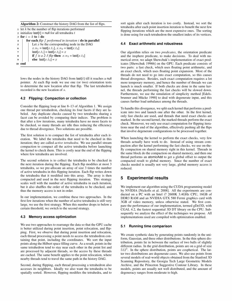
Algorithm 2: Construct the history DAG from the list of flips.
1 let k be the number of flip iterations performed2 initialize last[t] = null for all tetrahedra t3 for i = k to 1 do4 for each flip f performed in iteration i do in parallel5 Let x be the corresponding node in the DAG6 x.n1 = last[x.t1], x.n2 = last[x.t2]7 last[x.t1] = last[x.t2] = x8 if f is a 2-3 flip then x.n3 = last[x.t3]9 else last[x.t3] = x
10 end
lows the nodes in the history DAG from last[t] till it reaches a nullpointer. At each flip node we use one (or two) orientation teststo determine the new location after that flip. The last tetrahedronrecorded is the new location of s.
4.2 Flipping: Compaction or collection
Consider the flipping loop at line 8–13 of Algorithm 1. We assignone thread per tetrahedron, checking its four facets if they are la-beled. Any duplicate checks caused by two tetrahedra sharing afacet can be avoided by comparing their indices. The problem isthat after a few iterations, many tetrahedra have no more facets tobe checked, so many threads are idle thus reducing the efficiencydue to thread divergence. Two solutions are possible.
The first solution is to compact the list of tetrahedra after each it-eration. We label the tetrahedra that need to be checked in thisiteration; they are called active tetrahedra. We use parallel streamcompaction to compact all the active tetrahedra before launchingthe kernel to check them. This is costly near the end of the flippingwhere few tetrahedra are involved.
The second solution is to collect the tetrahedra to be checked inthe next iteration during the flipping. Each flip modifies at most 3tetrahedra, so we pre-allocate an array of size 3 times the numberof active tetrahedra in this flipping iteration. Each flip writes downthe tetrahedra that it modified into this array. The array is thencompacted and used in the next flipping iteration. This strategyscales well with the number of active tetrahedra in each iteration,but it also shuffles the order of the tetrahedra to be checked, andthus the memory access is not in order.
In our implementation, we combine these two approaches. In thefirst few iterations when the number of active tetrahedra is still verylarge, we use the first strategy. When this number drops to below acertain threshold, we switch to the second strategy.
4.3 Memory access optimization
We use two approaches to rearrange the data so that the GPU cacheis better utilized during point insertion, point relocation, and flip-ping. First, we observe that during point insertion and relocation,each thread processing a point needs to access the tetrahedron con-taining that point, including the coordinates. We sort the inputpoints along the Hilbert space filling curve. As a result, points in thesame tetrahedron tend to stay near each other in the point list andare processed by adjacent threads, so the access by these threadsare cached. The same benefit applies to the point relocation, wherenearby threads tend to travel the same path in the history DAG.
Second, during flipping, each thread processing a tetrahedron alsoaccesses its neighbors. Ideally we also want the tetrahedra to bespatially sorted. However, flipping modifies the tetrahedra, and to
sort again after each iteration is too costly. Instead, we sort thetetrahedra after each point insertion iteration to benefit the next fewflipping iterations which are the most expensive ones. The sortingis done using for each tetrahedron the smallest index of its vertices.
4.4 Exact arithmetic and robustness
Our algorithm relies on two predicates, the orientation predicateand the insphere predicate, to make decisions. To deal with nu-merical error, we adapt Shewchuk’s implementation of exact pred-icates [Shewchuk 1996b] on the GPU. Each predicate consists oftwo parts: a fast check, which uses floating point arithmetic, andan exact check, which uses floating point expansion. Most of thethreads do not need to go into exact computation, so this causesthread divergence. Besides, each exact computation requires a lotmore temporary memory, and hence the number of threads we canlaunch is much smaller. If both checks are done in the same ker-nel, the threads performing the fast checks will be slowed down.Furthermore, we use the simulation of simplicity method [Edels-brunner and Mucke 1990] to deal with degenerate input, and thiscauses further load unbalance among the threads.
To handle this divergence, we split each kernel that performs a pred-icate into two and launch one after the other. In the first kernel,only fast checks are used, and threads that need exact checks aremarked. In the second kernel, the marked threads perform the exactcheck. Moreover, we only use exact computation for flipping itera-tions near the end of the algorithm, effectively pushing all the flipsthat involve degenerate configurations to be processed together.
When launching the kernel to perform the exact checks, very fewthreads actually have work to do. Instead of using stream com-paction after the kernel performing the fast checks, we use on-the-fly compaction on shared memory right in this kernel. Threads inthe same block do the compaction on shared memory, and then onethread performs an atomicAdd to get a global offset to output thecompacted result to global memory. Since the number of exactchecks needed is usually not very large, global memory access isreduced.
5 Experimental results
We implement our algorithm using the CUDA programming modelby NVIDIA [Nickolls et al. 2008]. All the experiments are con-ducted on a PC with an Intel i7 2600K 3.4GHz CPU, 16GB ofDDR3 RAM and an NVIDIA GTX 580 Fermi graphics card with3GB of video memory, unless otherwise stated. We first com-pare the performance of our implementation, termed gDel3D, withCGAL 4.2, the fastest sequential 3D DT library on the CPU. Sub-sequently we analyze the effect of the techniques we propose. Allimplementations used are compiled with optimization enabled.
5.1 Running time comparison
We create synthetic data by generating points randomly in the uni-form, Gaussian, and three other distributions. In the thin sphere dis-tribution, points lie in between the surface of two balls of slightlydifferent radius. In the grid distribution, points are on a grid of size5123. In the sphere distribution, points are cospherical. The lat-ter two distributions are degenerate cases. We also use points fromseveral models of real-world objects obtained from the Stanford 3DScanning Repository, the Georgia Tech Large Geometric ModelsArchive, and the Princeton Suggestive Contour Library. In thesemodels, points are usually not well distributed, and the amount ofdegeneracy ranges from moderate to high.
Uniform Gaussian Thin sphere Grid Sphere
Model # Points
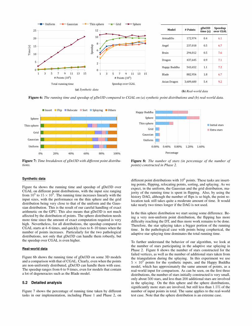
Armadillo 172,974 0.4 6.1
Angel 237,018 0.5 6.7
Brain 294,012 0.5 7.6
Dragon 437,645 0.9 7.1
Happy Buddha 543,652 1.1 7.2
Blade 882,954 1.8 6.7
Asian Dragon 3,609,600 5.4 9.2
gDel3Dtime (s)
Speedup over CGAL
(b) Real-world data
1 3 5 7 9 11 13 150
5
10
15
20
25
Total running time
# Points (10⁵)
Tim
e (s
)
1 3 5 7 9 11 13 150
2
4
6
8
10
12
Speedup over CGAL
# Points (10⁵)
Spee
dup
(a) Synthetic data
Figure 6: The running time and speedup of gDel3D compared to CGAL on (a) synthetic point distributions and (b) real-world data.
Insert Flip Relocate Sort Splaying Others
Uniform
Gaussian
Grid
Thin sphere
Sphere
0% 20% 40% 60% 80% 100%
Figure 7: Time breakdown of gDel3D with different point distribu-tions.
Synthetic data
Figure 6a shows the running time and speedup of gDel3D overCGAL on different point distributions, with the input size rangingfrom 105 to 15× 105. The running time increases linearly with theinput sizes, with the performance on the thin sphere and the griddistribution being very close to that of the uniform and the Gaus-sian distribution. This is the result of our careful handling of exactarithmetic on the GPU. This also means that gDel3D is not muchaffected by the distribution of points. The sphere distribution needsmore time since the amount of exact computation required is veryhigh. Nevertheless, for all distributions, the speedup compared toCGAL starts at 4–6 times, and quickly rises to 8–10 times when thenumber of points increases. Particularly for the two pathologicaldistributions, not only that gDel3D can handle them robustly, butthe speedup over CGAL is even higher.
Real-world data
Figure 6b shows the running time of gDel3D on some 3D modelsand a comparison with that of CGAL. Clearly, even when the pointsare non-uniformly distributed, gDel3D can handle them with ease.The speedup ranges from 6 to 9 times, even for models that containa lot of degeneracies such as the Blade model.
5.2 Detailed analysis
Figure 7 shows the percentage of running time taken by differenttasks in our implementation, including Phase 1 and Phase 2, on
Uniform
Gaussian
Grid
Thin sphere
Sphere
Happy Buddha
0.00% 0.40% 0.80% 1.20% 1.60%
Percentage
Initial stars
Extra stars
Figure 8: The number of stars (in percentage of the number ofpoints) constructed in Phase 2.
different point distributions with 106 points. These tasks are insert-ing points, flipping, relocating points, sorting, and splaying. As weexpect, in the uniform, the Gaussian and the grid distribution, ma-jority of the running time is spent in flipping. Also, by using thehistory DAG, although the number of flips is so high, the point re-location task still takes quite a moderate amount of time. It wouldtake nearly two times longer if the DAG is not used.
In the thin sphere distribution we start seeing some difference. Be-ing a very non-uniform point distribution, the flipping has moredifficulty reaching the DT, and thus more work remains to be done.Therefore, the star splaying takes a bigger portion of the runningtime. In the pathological case with points being cospherical, theadaptive star splaying time dominates the total running time.
To further understand the behavior of our algorithm, we look atthe number of stars participating in the adaptive star splaying inPhase 2. Figure 8 shows the number of stars constructed for thefailed vertices, as well as the number of additional stars taken fromthe triangulation during the splaying. In this experiment we use5 × 105 points for the synthetic inputs, and the Happy Buddhamodel, which has approximately the same amount of points, as areal-world input for comparison. As can be seen, on the first threedistributions, the number of stars initially constructed is very small,only about 500 stars, and less than 200 additional stars are involvedin the splaying. On the thin sphere and the sphere distributions,significantly more stars are involved, but still less than 1.5% of thenumber of input points in total. The same applies to the real-worldtest case. Note that the sphere distribution is an extreme case.
2 4 6 8 10
1E+0
1E+1
1E+2
1E+3
1E+4
1E+5InsFlip InsAll
# Points (10⁵)
# F
aile
d ve
rtic
es
(a) # Failed vertices
2 4 6 8 100
5
10
15
20
25
30
InsFlip InsAll
# Points (10⁵)#
Fli
ps (
10⁶)
(b) # Flips performed
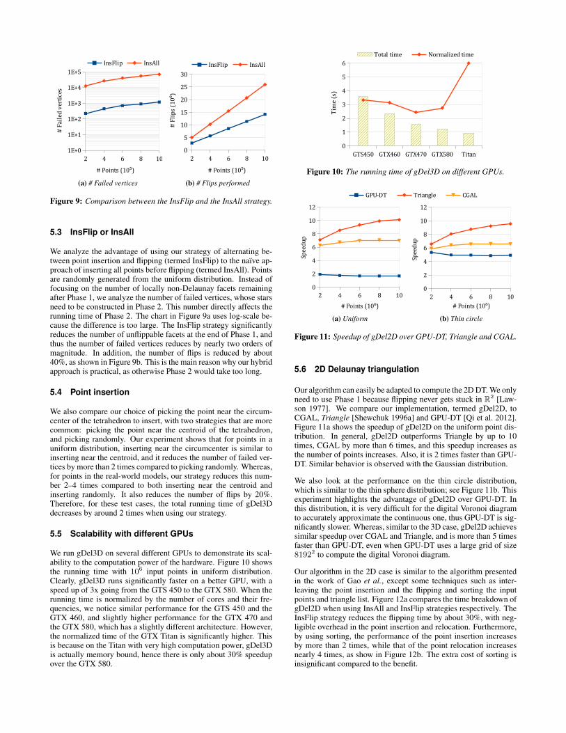
Figure 9: Comparison between the InsFlip and the InsAll strategy.
5.3 InsFlip or InsAll
We analyze the advantage of using our strategy of alternating be-tween point insertion and flipping (termed InsFlip) to the naıve ap-proach of inserting all points before flipping (termed InsAll). Pointsare randomly generated from the uniform distribution. Instead offocusing on the number of locally non-Delaunay facets remainingafter Phase 1, we analyze the number of failed vertices, whose starsneed to be constructed in Phase 2. This number directly affects therunning time of Phase 2. The chart in Figure 9a uses log-scale be-cause the difference is too large. The InsFlip strategy significantlyreduces the number of unflippable facets at the end of Phase 1, andthus the number of failed vertices reduces by nearly two orders ofmagnitude. In addition, the number of flips is reduced by about40%, as shown in Figure 9b. This is the main reason why our hybridapproach is practical, as otherwise Phase 2 would take too long.
5.4 Point insertion
We also compare our choice of picking the point near the circum-center of the tetrahedron to insert, with two strategies that are morecommon: picking the point near the centroid of the tetrahedron,and picking randomly. Our experiment shows that for points in auniform distribution, inserting near the circumcenter is similar toinserting near the centroid, and it reduces the number of failed ver-tices by more than 2 times compared to picking randomly. Whereas,for points in the real-world models, our strategy reduces this num-ber 2–4 times compared to both inserting near the centroid andinserting randomly. It also reduces the number of flips by 20%.Therefore, for these test cases, the total running time of gDel3Ddecreases by around 2 times when using our strategy.
5.5 Scalability with different GPUs
We run gDel3D on several different GPUs to demonstrate its scal-ability to the computation power of the hardware. Figure 10 showsthe running time with 106 input points in uniform distribution.Clearly, gDel3D runs significantly faster on a better GPU, with aspeed up of 3x going from the GTS 450 to the GTX 580. When therunning time is normalized by the number of cores and their fre-quencies, we notice similar performance for the GTS 450 and theGTX 460, and slightly higher performance for the GTX 470 andthe GTX 580, which has a slightly different architecture. However,the normalized time of the GTX Titan is significantly higher. Thisis because on the Titan with very high computation power, gDel3Dis actually memory bound, hence there is only about 30% speedupover the GTX 580.
GTS450 GTX460 GTX470 GTX580 Titan0
1
2
3
4
5
6Total time Normalized time
Tim
e (s
)
Figure 10: The running time of gDel3D on different GPUs.
GPU-DT Triangle CGAL
2 4 6 8 10
0
2
4
6
8
10
12
# Points (10⁶)Sp
eedu
p
(a) Uniform
2 4 6 8 10
0
2
4
6
8
10
12
# Points (10⁶)
Spee
dup
(b) Thin circle
Figure 11: Speedup of gDel2D over GPU-DT, Triangle and CGAL.
5.6 2D Delaunay triangulation
Our algorithm can easily be adapted to compute the 2D DT. We onlyneed to use Phase 1 because flipping never gets stuck in R2 [Law-son 1977]. We compare our implementation, termed gDel2D, toCGAL, Triangle [Shewchuk 1996a] and GPU-DT [Qi et al. 2012].Figure 11a shows the speedup of gDel2D on the uniform point dis-tribution. In general, gDel2D outperforms Triangle by up to 10times, CGAL by more than 6 times, and this speedup increases asthe number of points increases. Also, it is 2 times faster than GPU-DT. Similar behavior is observed with the Gaussian distribution.
We also look at the performance on the thin circle distribution,which is similar to the thin sphere distribution; see Figure 11b. Thisexperiment highlights the advantage of gDel2D over GPU-DT. Inthis distribution, it is very difficult for the digital Voronoi diagramto accurately approximate the continuous one, thus GPU-DT is sig-nificantly slower. Whereas, similar to the 3D case, gDel2D achievessimilar speedup over CGAL and Triangle, and is more than 5 timesfaster than GPU-DT, even when GPU-DT uses a large grid of size81922 to compute the digital Voronoi diagram.
Our algorithm in the 2D case is similar to the algorithm presentedin the work of Gao et al., except some techniques such as inter-leaving the point insertion and the flipping and sorting the inputpoints and triangle list. Figure 12a compares the time breakdown ofgDel2D when using InsAll and InsFlip strategies respectively. TheInsFlip strategy reduces the flipping time by about 30%, with neg-ligible overhead in the point insertion and relocation. Furthermore,by using sorting, the performance of the point insertion increasesby more than 2 times, while that of the point relocation increasesnearly 4 times, as show in Figure 12b. The extra cost of sorting isinsignificant compared to the benefit.
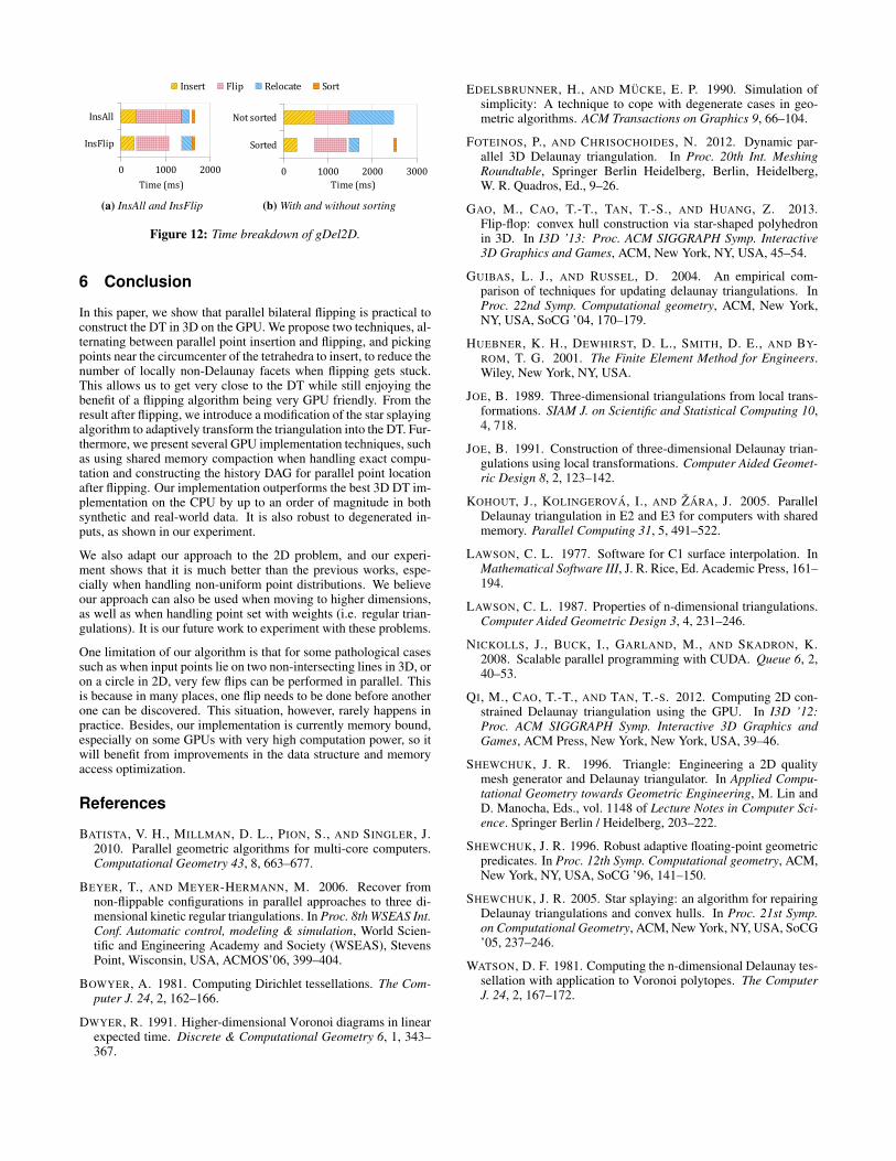
Insert Flip Relocate Sort
InsFlip
InsAll
0 1000 2000
Time (ms)
(a) InsAll and InsFlip
Sorted
Not sorted
0 1000 2000 3000Time (ms)
(b) With and without sorting
Figure 12: Time breakdown of gDel2D.
6 Conclusion
In this paper, we show that parallel bilateral flipping is practical toconstruct the DT in 3D on the GPU. We propose two techniques, al-ternating between parallel point insertion and flipping, and pickingpoints near the circumcenter of the tetrahedra to insert, to reduce thenumber of locally non-Delaunay facets when flipping gets stuck.This allows us to get very close to the DT while still enjoying thebenefit of a flipping algorithm being very GPU friendly. From theresult after flipping, we introduce a modification of the star splayingalgorithm to adaptively transform the triangulation into the DT. Fur-thermore, we present several GPU implementation techniques, suchas using shared memory compaction when handling exact compu-tation and constructing the history DAG for parallel point locationafter flipping. Our implementation outperforms the best 3D DT im-plementation on the CPU by up to an order of magnitude in bothsynthetic and real-world data. It is also robust to degenerated in-puts, as shown in our experiment.
We also adapt our approach to the 2D problem, and our experi-ment shows that it is much better than the previous works, espe-cially when handling non-uniform point distributions. We believeour approach can also be used when moving to higher dimensions,as well as when handling point set with weights (i.e. regular trian-gulations). It is our future work to experiment with these problems.
One limitation of our algorithm is that for some pathological casessuch as when input points lie on two non-intersecting lines in 3D, oron a circle in 2D, very few flips can be performed in parallel. Thisis because in many places, one flip needs to be done before anotherone can be discovered. This situation, however, rarely happens inpractice. Besides, our implementation is currently memory bound,especially on some GPUs with very high computation power, so itwill benefit from improvements in the data structure and memoryaccess optimization.
References
BATISTA, V. H., MILLMAN, D. L., PION, S., AND SINGLER, J.2010. Parallel geometric algorithms for multi-core computers.Computational Geometry 43, 8, 663–677.
BEYER, T., AND MEYER-HERMANN, M. 2006. Recover fromnon-flippable configurations in parallel approaches to three di-mensional kinetic regular triangulations. In Proc. 8th WSEAS Int.Conf. Automatic control, modeling & simulation, World Scien-tific and Engineering Academy and Society (WSEAS), StevensPoint, Wisconsin, USA, ACMOS’06, 399–404.
BOWYER, A. 1981. Computing Dirichlet tessellations. The Com-puter J. 24, 2, 162–166.
DWYER, R. 1991. Higher-dimensional Voronoi diagrams in linearexpected time. Discrete & Computational Geometry 6, 1, 343–367.
EDELSBRUNNER, H., AND MUCKE, E. P. 1990. Simulation ofsimplicity: A technique to cope with degenerate cases in geo-metric algorithms. ACM Transactions on Graphics 9, 66–104.
FOTEINOS, P., AND CHRISOCHOIDES, N. 2012. Dynamic par-allel 3D Delaunay triangulation. In Proc. 20th Int. MeshingRoundtable, Springer Berlin Heidelberg, Berlin, Heidelberg,W. R. Quadros, Ed., 9–26.
GAO, M., CAO, T.-T., TAN, T.-S., AND HUANG, Z. 2013.Flip-flop: convex hull construction via star-shaped polyhedronin 3D. In I3D ’13: Proc. ACM SIGGRAPH Symp. Interactive3D Graphics and Games, ACM, New York, NY, USA, 45–54.
GUIBAS, L. J., AND RUSSEL, D. 2004. An empirical com-parison of techniques for updating delaunay triangulations. InProc. 22nd Symp. Computational geometry, ACM, New York,NY, USA, SoCG ’04, 170–179.
HUEBNER, K. H., DEWHIRST, D. L., SMITH, D. E., AND BY-ROM, T. G. 2001. The Finite Element Method for Engineers.Wiley, New York, NY, USA.
JOE, B. 1989. Three-dimensional triangulations from local trans-formations. SIAM J. on Scientific and Statistical Computing 10,4, 718.
JOE, B. 1991. Construction of three-dimensional Delaunay trian-gulations using local transformations. Computer Aided Geomet-ric Design 8, 2, 123–142.
KOHOUT, J., KOLINGEROVA, I., AND ZARA, J. 2005. ParallelDelaunay triangulation in E2 and E3 for computers with sharedmemory. Parallel Computing 31, 5, 491–522.
LAWSON, C. L. 1977. Software for C1 surface interpolation. InMathematical Software III, J. R. Rice, Ed. Academic Press, 161–194.
LAWSON, C. L. 1987. Properties of n-dimensional triangulations.Computer Aided Geometric Design 3, 4, 231–246.
NICKOLLS, J., BUCK, I., GARLAND, M., AND SKADRON, K.2008. Scalable parallel programming with CUDA. Queue 6, 2,40–53.
QI, M., CAO, T.-T., AND TAN, T.-S. 2012. Computing 2D con-strained Delaunay triangulation using the GPU. In I3D ’12:Proc. ACM SIGGRAPH Symp. Interactive 3D Graphics andGames, ACM Press, New York, New York, USA, 39–46.
SHEWCHUK, J. R. 1996. Triangle: Engineering a 2D qualitymesh generator and Delaunay triangulator. In Applied Compu-tational Geometry towards Geometric Engineering, M. Lin andD. Manocha, Eds., vol. 1148 of Lecture Notes in Computer Sci-ence. Springer Berlin / Heidelberg, 203–222.
SHEWCHUK, J. R. 1996. Robust adaptive floating-point geometricpredicates. In Proc. 12th Symp. Computational geometry, ACM,New York, NY, USA, SoCG ’96, 141–150.
SHEWCHUK, J. R. 2005. Star splaying: an algorithm for repairingDelaunay triangulations and convex hulls. In Proc. 21st Symp.on Computational Geometry, ACM, New York, NY, USA, SoCG’05, 237–246.
WATSON, D. F. 1981. Computing the n-dimensional Delaunay tes-sellation with application to Voronoi polytopes. The ComputerJ. 24, 2, 167–172.