
A Goal-Directed Shortest Path Algorithm Using Precomputed Cluster...
70
A Goal-Directed Shortest Path Algorithm Using Precomputed Cluster Distances Jens Maue Diplomarbeit · Diploma Thesis Department of Computer Science Saarland University, Saarbr¨ ucken June 2006 Topic by Prof. Dr. Kurt Mehlhorn, Max-Planck-Institut f¨ ur Informatik, Saarbr¨ ucken Supervised by Prof. Dr. Peter Sanders, Universit¨ at Karlsruhe (TH)
Transcript of A Goal-Directed Shortest Path Algorithm Using Precomputed Cluster...
A Goal-Directed Shortest Path AlgorithmUsing Precomputed Cluster Distances
Jens Maue
Diplomarbeit · Diploma Thesis
Department of Computer Science
Saarland University, Saarbrucken
June 2006
Topic by Prof. Dr. Kurt Mehlhorn, Max-Planck-Institut fur Informatik, SaarbruckenSupervised by Prof. Dr. Peter Sanders, Universitat Karlsruhe (TH)


Hiermit versichere ich, dass ich diese Arbeit selbststandig verfasst und keine anderen alsdie angegebenen Quellen und Hilfsmittel benutzt habe.
Saarbrucken, im Juni 2006
Acknowledgements
First of all, I would like to thank Peter Sanders for all the help and encouragementprovided while supervising my thesis. Furthermore, many thanks to Dominik Schultes forsupplying me with graph instances and corresponding conversion tools, and to MichaelKaißer, Soren Laue, and Domagoj Matijevic for proof reading my thesis carefully. Lastbut not least, I would like to thank Kurt Mehlhorn for his readiness to examine thisthesis.


Abstract
This thesis introduces a new acceleration heuristic for shortest path queries, called thePCD algorithm (Precomputed Cluster Distances). PCD precomputes shortest pathdistances between the partitions of the input graph, which can be obtained by any graphpartitioning method. Since the number of partitions can be varied between one and thenumber of nodes, the method presents an interpolation between all pairs and ordinarysingle source single target shortest path search. This allows a flexible trade-off betweenpreprocessing time and space on the one hand and query time on the other, allowingsignificant speedups even for a sublinear amount of extra space. The method can beapplied to arbitrary graphs with non-negative edge weights and does not afford a layout.Experiments on large street networks with a suitable clustering method are shown toyield average speedups of up to 114.9 for PCD as a stand-alone method. Furthermore,the algorithm’s space-efficiency, simplicity, and goal-directed behaviour make PCD analternative method to provide other acceleration heuristics with goal-direction.


Contents
1 Introduction 1
1.1 Motivation . . . . . . . . . . . . . . . . . . . . . . . . . . . . . . . . . . . 1
1.2 Related Work . . . . . . . . . . . . . . . . . . . . . . . . . . . . . . . . . 2
1.3 Precomputed Cluster Distances (PCD) . . . . . . . . . . . . . . . . . . . 7
1.4 Outline . . . . . . . . . . . . . . . . . . . . . . . . . . . . . . . . . . . . . 10
2 Preliminaries 11
2.1 Graphs and Paths . . . . . . . . . . . . . . . . . . . . . . . . . . . . . . . 11
2.2 The Shortest Paths Problem and Dijkstra’s Algorithm . . . . . . . . . . 12
2.3 Graph Partitioning . . . . . . . . . . . . . . . . . . . . . . . . . . . . . . 14
2.4 The k-Center Problem . . . . . . . . . . . . . . . . . . . . . . . . . . . . 15
3 PCD Part 1: Preprocessing 16
3.1 Cluster Ids and Border Nodes . . . . . . . . . . . . . . . . . . . . . . . . 16
3.2 Computing the Cluster Distances . . . . . . . . . . . . . . . . . . . . . . 16
3.3 Initialising the Query . . . . . . . . . . . . . . . . . . . . . . . . . . . . . 18
4 PCD Part 2: Query 19
4.1 The PCD Query Algorithm . . . . . . . . . . . . . . . . . . . . . . . . . 19
4.2 The Unidirectional Version . . . . . . . . . . . . . . . . . . . . . . . . . . 28
4.3 Upper Bounds at Cluster Entry . . . . . . . . . . . . . . . . . . . . . . . 29
5 PCD Part 0: Partitioning 31
5.1 k-Center Clustering . . . . . . . . . . . . . . . . . . . . . . . . . . . . . . 31
5.2 Grid Clustering . . . . . . . . . . . . . . . . . . . . . . . . . . . . . . . . 38
5.3 METIS . . . . . . . . . . . . . . . . . . . . . . . . . . . . . . . . . . . . . . 39
5.4 Cluster Radii . . . . . . . . . . . . . . . . . . . . . . . . . . . . . . . . . 39

6 Experiments 40
6.1 Test Instances . . . . . . . . . . . . . . . . . . . . . . . . . . . . . . . . . 40
6.2 Experimental Setup . . . . . . . . . . . . . . . . . . . . . . . . . . . . . . 41
6.3 Experimental Results . . . . . . . . . . . . . . . . . . . . . . . . . . . . . 42
7 Concluding Remarks 53
7.1 Conclusion . . . . . . . . . . . . . . . . . . . . . . . . . . . . . . . . . . . 53
7.2 Future Work . . . . . . . . . . . . . . . . . . . . . . . . . . . . . . . . . . 54
Appendix 56
A condensed version of this thesis can be found in [MSM06], which is a joint work withPeter Sanders and Domagoj Matijevic.

Chapter 1
Introduction
This chapter introduces the problem this thesis deals with and gives an overview ofrelated approaches. Then, it briefly describes the new method of Precomputed ClusterDistances (PCD), followed by an outline of the thesis.
1.1 Motivation
Computing the shortest path between two points in a network is one of the most funda-mental algorithmic problems. There are many real-world applications that translate tothis problem, one of which is answering optimal-path queries in route planning systemssuch as timetable information services for public transport or car navigation systems.
A well studied and widely used algorithm for shortest paths problems is Dijkstra’s al-gorithm [Dij59]. Though Dijkstra’s algorithm is fast regarding the worst case runningtime, it is often too slow for answering single-source single-target queries, particularlyfor applications to large graphs with frequent queries.
In the typical application scenarios, the queries are to be answered exact and quickly,and there are usually many queries while the network does not change. This motivates toperform some amount of preprocessing in order to improve the query times. Naturally,precomputing and storing the shortest paths for all possible queries would result inconstant time queries. But, this approach is prohibited by its huge time requirementsince traffic networks sometimes do change, and the quadratic space requirement is notaffordable either, which holds for large graphs in particular.
Therefore, the preprocessing has to work reasonably fast, and the amount of preprocesseddata should not exceed that of of the input. On the other hand, the queries ought to beeffectively accelerated independently of the graph size. These aspects present conflictingobjectives, and to allow adjusting the trade-off between them is a desirable feature of apossible algorithm.
To sum up, this thesis focuses on exact single-source single-target shortest path querieson large street networks. The main goals are fast queries on a temporarily static graphwithout a layout, using a fast preprocessing that stores a small and adjustable amountof auxiliary data.
1

2 CHAPTER 1. INTRODUCTION
Dijkstra’s algorithm
↓Speedup heuristics
↓No Preprocessing
• bidirected search
• A∗ search
↓Preprocessing
Goal-Directed
• Landmark-A∗
• GeometricContainers
• Edge-Flags
• PCD
Hierarchical
• Seperator-BasedMulti-Level
• HighwayHierarchies
• Reach-BasedPruning
↓Combinations
• bidirected A∗
• Landmarks+ Reaches
• other
Figure 1.1: Overview of the shortest path algorithms and speedup heuristics introducedin this section.
1.2 Related Work
A huge amount of research concerning shortest paths and related problems has beendone in the recent past, and the main results related to PCD are presented in thefollowing. This particularly includes speedup heuristics based on Dijkstra’s algorithm;Figure 1.1 gives an overview of the presented techniques. Most of them perform someprecomputation on the input data to speed up the search as motivated above. Theyall present different solutions to the problem of balancing between preprocessing time,additional space, and query performance. The latter can be rated by a method’s speedup,which denotes the factor by which an average query outperforms a search with Dijkstra’salgorithm in terms of query time or size of the search space.
Dijkstra’s Algorithm
The best-known and most commonly used shortest path algorithm is that of Dijk-stra [Dij59], which solves the single-source shortest paths problem for directed graphswith non-negative edge weights. Dijkstra’s algorithm is efficiently implemented by us-ing a priority queue, on which n insertions, n deletions, and m decrease-key operationsare performed, so the actual running time depends on how this priority queue is imple-mented. The Fibonacci heap data structure allows insert and decrease-key operationsin constant and deleting in O(log n) amortised time, which yields a running time ofO(m + n log n) [FT87].
1.2. RELATED WORK 3
s t
(a) Dijkstra’s algorithm
s t
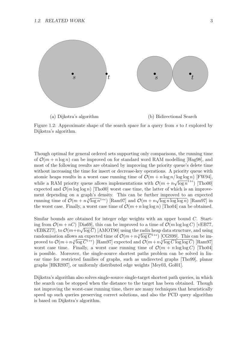
(b) Bidirectional Search
Figure 1.2: Approximate shape of the search space for a query from s to t explored byDijkstra’s algorithm.
Though optimal for general ordered sets supporting only comparisons, the running timeof O(m + n log n) can be improved on for standard word RAM modelling [Hag98], andmost of the following results are obtained by improving the priority queue’s delete timewithout increasing the time for insert or decrease-key operations. A priority queue withatomic heaps results in a worst case running time of O(m + n log n/ log log n) [FW94],
while a RAM priority queue allows implementations with O(m + n√
log n1+ε
) [Tho00]expected and O(m log log n) [Tho00] worst case time, the latter of which is an improve-ment depending on a graph’s density. This can be further improved to an expectedrunning time of O(m + n 3
√log n1+ε) [Ram97] and O(m + n
√log n log log n) [Ram97] in
the worst case. Finally, a worst case time of O(m+n log log n) [Tho04] can be obtained.
Similar bounds are obtained for integer edge weights with an upper bound C. Start-ing from O(m + nC) [Dia69], this can be improved to a time of O(m log log C) [vEB77,vEBKZ77], toO(m+n
√log C) [AMOT90] using the radix heap data structure, and using
randomisation allows an expected time of O(m+n 3√
log C1+ε) [CGS99]. This can be im-proved to O(m+n 4
√log C1+ε) [Ram97] expected and O(m+n 3
√log C log log C) [Ram97]
worst case time. Finally, a worst case running time of O(m + n log log C) [Tho04]is possible. Moreover, the single-source shortest paths problem can be solved in lin-ear time for restricted families of graphs, such as undirected graphs [Tho99], planargraphs [HKRS97], or uniformly distributed edge weights [Mey03, Gol01].
Dijkstra’s algorithm also solves single-source single-target shortest path queries, in whichthe search can be stopped when the distance to the target has been obtained. Thoughnot improving the worst-case running time, there are many techniques that heuristicallyspeed up such queries preserving correct solutions, and also the PCD query algorithmis based on Dijkstra’s algorithm.

4 CHAPTER 1. INTRODUCTION
s t
(a) A∗ Search
s t
(b) PCD
Figure 1.3: Approximate search space of A∗ search compared with the PCD algorithm.
Search Heuristics
A quite simple acceleration technique not affording any additional information such asa graph layout or preprocessed data is bidirectional search [Poh71]. This simultaneouslyexplores the reverse graph from the target and finishes when the search frontiers meetas sketched in Figure 1.2. As a rule of thumb, the search space of Dijkstra’s algorithmis usually considered to grow by the square of the path distance for road networks, sobidirectional search can be expected to yield a speedup of two: if Dijkstra’s algorithm
explores p2 nodes for a path of length p, its bidirectional version searches 2 ·(
p2
)2= p2
2
nodes, i.e. half the number. The PCD query algorithm also applies bidirectional search.
The goal-directed A∗ algorithm [HNR68, HNR72] reduces the search space by prefer-ring nodes which are on a path with a low length estimate: given a potential functionπt : V → IR, A∗ repeatedly selects the node u whose estimate d(s, u) + πt(u) is thesmallest; the resulting search space is shown in Figure 1.3. A∗ corresponds to Dijk-stra’s algorithm in the following way: the reduced weight wπt(e) of an edge e = (u, v)is defined by wπt(e) = w(e) − πt(u) + πt(v), and a potential function is called consis-tent if the reduced weight function is non-negative. For a consistent potential function,running the A∗ algorithm is equivalent to running Dijkstra’s algorithm on the graphwith reduced edge weights, whereas Dijkstra’s algorithm can be regarded as A∗ withthe zero-potential function. Euclidean distances provide a consistent potential function,but require the input graph featuring node coordinates and perform not very well forquickest path queries. Unfortunately, the cluster distances precomputed by PCD donot provide a consistent potential function for A∗, but also PCD shows goal-directedbehaviour; different from A∗, this is achieved by pruning.
Goal-Directed Preprocessing Heuristics
The following methods are also goal-directed, but they perform some preprocessingunlike A∗. They are summarised in Figure 1.1; PCD is an algorithm of this categorytoo.
The concept of landmarks provides a lower bounding technique for A∗ which is inde-pendent of node coordinates [GH05, GH04]. In a preprocessing step, a small numberof landmark nodes is selected, and the distances d(u, L) and d(L, u) to and from eachlandmark L is computed for every node u. Then, for two nodes u and t, lower bounds ford(u, t) are given by d(L, t)−d(L, u) and d(u, L)−d(t, L) for every landmark L by the tri-angle inequality. This is used in the query which follows the A∗ algorithm. Using only 16landmark nodes, a bidirectional implementation achieves a good speedup of 50 in terms

1.2. RELATED WORK 5
PreprocessingMethod Time Space Speedup
Landmarks Θ(l·D(n))a ++ Θ(l·n) −− 50 (l=16) +Geom. Containers Θ(n·D(n)) −− Θ(m) ◦ 30 +Edge Flags Θ(B ·D(n))b − Θ(k ·m) bitsc − 1,400 (k=225) ++PCD Θ(k ·D(n))b + Θ(k2+B) ++ 114.9 (k=212) +
anot including landmark selection; may increase depending on selection scheme [GW05]bnot including clusteringccan be reduced through hierarchical clustering [MSS+05]
Table 1.1: Speedups and preprocessing costs of goal-directed preprocessing heuristics.k denotes the number of clusters, l the number of landmarks, n the number of nodes,m the number of edges, B the number of border nodes, and D(n) the running time ofDijkstra’s algorithm.
of average number of settled nodes on a road network of about 6.7 million nodes. Thepreprocessing is fast since it performs only one shortest path search from each landmark(two for directed graphs). Still, sophisticated landmark selection strategies [GW05] canincrease the preprocessing time significantly. Furthermore, though linear in the num-ber of nodes for a constant number of landmarks, the additional space requirement isquite high since two distance values are stored for each node-landmark pair. The PCDalgorithm may afford more preprocessing than landmarks, but it achieves goal-directionmore space-efficiently through the adjustable number of clusters k.
If a graph is provided with a geometric layout, Dijkstra’s algorithm can be directedusing geometric containers requiring a linear amount of additional space: for each edgeof the input graph, a geometric object is preprocessed that covers all nodes to which ashortest path starts with this edge. Edges not relevant for the target node are omittedin the query. Angular sectors are used in [SWW00] with timetable information systems,while high speedups of about 30 in terms of size of the search space are obtained evenfor simpler geometric objects such as bounding boxes [WW03]. Updating containers indynamic graphs is dealt with in [WWZ05, WWZ04]. Though showing good speedups,preprocessing geometric containers affords one single source shortest path search fromevery node, which is prohibitive for larger graphs.
An approach similar to geometric containers is based on the concept of edge flags [Lau04,KMS05, MSS+05]: the input graph is partitioned, and a flag is computed for each edgeand each partition indicating whether the edge is contained in a shortest path to any nodeof this partition. The query only considers edges whose flag corresponding to the targetregion is set. The original approach used variants of grid partitioning [Lau04], whileapplied to partitionings obtained by METIS [Met95] (see Section 5.3 for a description ofMETIS) the approach yields excellent speedups of up to 1,400 for a road network of aboutone million nodes and 225 partitions [KMS05]. An extension to multiple levels furtheraccelerates unidirectional search without increasing the space requirement [MSS+05].Though lower than for geometric containers, the preprocessing time is still high sinceexecuting one shortest path search from every border node of every partition is necessary.For a road-network of 475,000 nodes and 100 partitions, this takes 2.5 hours [KMS05].

6 CHAPTER 1. INTRODUCTION
Hierarchical Preprocessing Heuristics
The following speedup techniques try to accelerate queries by restricting the search toa small subgraph. The preprocessing builds sparser and sparser levels above the inputgraph, to which the search algorithm repeatedly switches.
The separator-based multi-level approach precomputes some short shortest paths in orderto accelerate longer shortest path queries [Fre87, SWW00, SWZ02, HSW04, KMS05]:the input graph is partitioned along a node separator, and every separator node isdefined a border node of all partitions adjacent to it. Then, all shortest paths betweenborder nodes of the same region are precomputed, and an edge with the correspondingweight is introduced for each such path. These shortcut edges can be used by the queryalgorithm. Regarding the separator nodes with the edges connecting them as a secondlevel of the graph, the preprocessing can be applied repeatedly resulting in a multi-levelgraph. Obviously, preprocessing time, space requirement, and query times depend onthe small size of the node separator, and speedups of up to 14 are reported for a two-levelimplementation applied to street networks [KMS05]. In [SWZ02] a multi-level methodis shown to improve timetable information queries by a factor of eleven for four levels.
A different way of preprocessing a multi-level graph is that of highway hierarchies [SS05,Sch05], which rates the nodes of an input graph according to some locality parameter H:a node is called local if, for every shortest path it belongs to, the node is reached withinH steps by a shortest path search starting from the path’s source. This is appliediteratively in the preprocessing algorithm, which raises nodes to higher levels if they arenot local with respect to the current level. Furthermore, lines of nodes with a degreeof two are contracted into shortcut edges, so that levels are the sparser the higher theyare. The query repeatedly switches to higher levels of the graph, restricting the searchto a smaller subgraph. The method yields excellent speedups of up to 2,650 (3,000 interms of number of settled nodes), achieved for a road network with about 24 millionnodes and a reasonable preprocessing time of 4.25 hours.
A pruning algorithm affording a linear amount of additional space is based on the conceptof reach [Gut04]: intuitively, the reach of a node is large if the node is in the middle ofsome long shortest path. This is used in a query to prune nodes whose precomputedreach value is too small for the node to be on the shortest path currently searched.Since estimating exact reaches affords an all pairs shortest paths computation, whichis prohibitive for large graphs, upper bounds of the reaches can be estimated, affectingthe query performance but not correctness. Reach-based pruning shows speedups of upto 2,000 in terms of settled nodes and 1,475 in terms of query time for a road networkwith about 24 million nodes [GKW06, GKW05]. This is achieved by a bidirectional,self-bounding implementation with precomputed shortcut edges, affording a moderatepreprocessing time of about six hours.
Geometric information is required for some methods, such as geometric containers, graphpartitioning techniques from computational geometry, and A∗ search using Euclideandistances. Artificial node coordinates can be generated with methods from graph draw-ing [WW05, BSWW04] in order o apply these techniques if a layout is missing.

1.3. PRECOMPUTED CLUSTER DISTANCES (PCD) 7
Combinations
Most preprocessing heuristics can be combined with bidirectional search, and also com-bining bidirected search with A∗ can be beneficial [Poh71, KK97]. Both techniquescan be used together with the multi-level approach and geometric containers [HSW04,SWW00], and reach-based pruning combines with Euclidean-based A∗ in a straight-forward way [Gut04].
One of the currently most successful combinations is that of reach-based pruning andlandmark-based A∗, which yields average speedups of up to 3,600 (8,646 in terms of num-ber of settled nodes) [GKW06, GKW05]. The preprocessing time of almost eight hoursfor this adds up from computing the landmarks and the upper bounds on reaches, butthe distance between nodes and landmarks must still be stored, resulting in a high spacerequirement. Applying the self-bounding reach-based pruning algorithm mentioned be-fore is not possible with A∗ search.
Therefore, combining reach-based pruning with PCD instead of landmark-based A∗ ap-pears promising. This would allow implicit bounding and reduce the space requirement.Also, the tuning parameter k, i.e. the number of clusters, offers more flexibility in ad-justing preprocessing time and space than varying the number of landmarks. PCD alsoprovides a way to supply highway hierarchies with goal-directed behaviour in order toimprove their performance using only little more space, and the adjustable number ofclusters k extends the method by an additional tuning parameter.
1.3 Precomputed Cluster Distances (PCD)
The PCD algorithm presents another goal-directed speedup heuristic which uses pre-processing (see Figure 1.1). The number of settled nodes can be reduced significantly, asimplified picture of the resulting search space is shown in Figure 1.3.
Algorithm Summary
As outlined in Figure 1.4, PCD comprises two parts, the preprocessing and the queryalgorithm, and can be combined with any graph partitioning method. The preprocessingalgorithm expects a weighted graph as its input, which has been partitioned into kclusters, and computes and stores the distances between all k2 pairs of clusters.
These precomputed cluster distances are used during the query to maintain an upperbound of the shortest path distance, and they provide lower bounds for the remainingdistance from a node to the target. If the lower estimate for a node exceeds the currentupper bound, this node cannot be a member of the shortest path and is therefore pruned.
The upper bound always represents the length of an actual path—not necessarily theshortest—from the source to the target. Such a path is discovered whenever the firstnode on a precomputed shortest path to the target cluster is reached and the distancefrom this path’s last node to the target has been estimated by a backward search. Theupper bound holds the length of the shortest such path found so far. Figure 1.5 illustratesthis situation.

8 CHAPTER 1. INTRODUCTION
Partitioning
PCD
Preprocessing
Query
First Query Phase
Second Query Phase
?
Figure 1.4: Components of PCD featuring the preprocessing and the query part. Thepreceding partitioning algorithm can be chosen independently of PCD.
U
S Ts
t
tUT
sUTd(s, sUT)d(U, T )
d(tUT , t)
Figure 1.5: Updating the upper bound of the shortest path distance from s to t whensettling the first node sUT of a precomputed path from U to T .

1.3. PRECOMPUTED CLUSTER DISTANCES (PCD) 9
u
U
S Ts tUT
sUT
t′
d(s, u)d(U, T )
t
d(t′, t)
1stphase
Figure 1.6: Estimating a lower bound for the length of any path from s to t containingu. The border node t′ of T which is the closest to t has been determined by the end ofthe first query phase.
For every settled node u, a lower bound is estimated as shown in Figure 1.6. The lengthof any path from the source s to target t containing u can be bounded from below by thesum of the following three values: the distance d(s, u) from s to u, which has just beenfound by settling u, the precomputed distance from u’s cluster U to the target clusterT , and the minimum distance from the border of T to t.
When the lower bound d(s, u, t) is estimated for some node u ∈ U , the distance betweenu and the start node sUT of the precomputed path from U to the target cluster T cannotbe bounded from below. Hence, there is a ‘gap’ in the lower bound estimate for u, whosevalue depends on the diameter of U . Another gap can be found in the target cluster:the minimum distance from the target to the border might be close to zero while theshortest path crosses the whole cluster. This difference can be as big as the diameter ofthe target cluster. Since increasing the number of clusters k decreases the average clusterdiameter, the choice of k affects the quality of the lower bound estimates. Furthermore,choosing a sensible partitionining method in order to reduce the average diameter has ahigh effect on the lower bounds independently of the number of clusters.
Advantages over Related Methods
Similar to the edge flag approach and multi-level graph decomposition, the number ofclusters k can be adjusted to decrease the costs of preprocessing. However, the prepro-cessing time for PCD is independent of the number of border nodes, and thus indepen-dent of the partitioning method, since exactly k single source shortest path computationsare performed. In contrast, the edge flag approach requires one shortest path search fromevery border node of every cluster. Also, PCD achieves high speedups even for a simpleclustering method such as grid clustering, while the performance of the separator-basedmultilevel method highly depends on the size of the separator. Furthermore, suitablychoosing the number of clusters allows an amount of preprocessed data sublinear in theinput graph size unlike, for example, the landmark method. Moreover, PCD does notrequire graphs provided with a layout in contrast to geometric pruning, though parti-tionings might still be obtained by techniques from computational geometry if a layout

10 CHAPTER 1. INTRODUCTION
is given. The preprocessing costs and average speedups of PCD are compared to othergoal-directed methods in Table 1.1.
1.4 Outline
Chapter 2 introduces the definitions and concepts related to PCD, which are thoseof the shortest path problem in general, Dijkstra’s algorithm, and graph partitioning.Furthermore, the k-center problem and its relation to graph partitioning is described.
Chapter 3 explains the preprocessing algorithm, which constitutes the first part of PCD.The first issue is how to handle cluster information space-efficiently without increasingthe preprocessing time, followed by the preprocessing’s main part of precomputing thecluster distances.
Chapter 4 contains a detailed description of the PCD query algorithm with its twoconsecutive phases. The bidirectional variant is presented first, including its proof ofcorrectness and a more detailed illustration of the bounding method. Then, the unidi-rectional query algorithm is outlined as well as a variant for estimating upper bounds.
Chapter 5 presents several graph partitioning algorithms used to provide the preprocess-ing with some clustering. Particularly, the notion of k-center clustering is introduced aswell as several ways to obtain this.
Chapter 6 contains the experimental evaluation of PCD using large real-world graphinstances. Query performance, space requirement, and preprocessing time are examined,and how these results are affected by varying the graph partitioning method, by differentedge weight functions, and by the amount of preprocessing in particular. The appendixcontains further measurement data connected to this.
Chapter 7 summarises the main results and outlines possible future work related toPCD. This includes different graph partitioning algorithms, improvements of the queryalgorithm itself, and combining it with other speedup heuristics. The latter particularlyincludes a combination with highway hierarchies and with reach-based pruning in placeof landmarks.

Chapter 2
Preliminaries
This chapter introduces the terminology and basic concepts used throughout this thesissuch as the notion of a graph, several variants of the shortest paths problem, and Dijk-stra’s algorithm. Furthermore, the problem of graph partitioning is presented as well asthe related k-center problem.
2.1 Graphs and Paths
A directed graph G is a a pair (V, E), where V is a finite set and E ⊆ V ×V . An elementof V is called a node of G, an element of E is called an edge, and n := |V | and m := |E|denote their numbers. If m = O(n), a graph is called sparse. In an undirected graph theset of edges is given by E ⊆ {{u, v} |u, v ∈ V, u 6= v}. Furthermore, a weight functionw : E → IR≥0 associated with the edge set is assumed to be given for any (undirected)graph. For any edge e ∈ E, the number w(e) is then called the weight of e.
Note: In this thesis graphs will implicitly be assumed to be undirected and thus do notcontain any self-loops or parallel edges by the definition above. Self-loops and paralleledges can be deleted in a preprocessing step in linear time O(m), where for each set ofparallel edges the edge with the lowest weight is kept. Also, edge weights are expectednon-zero as zero-weight edges can be easily dealt with by merging their end nodes.Moreover, for better readability, the edges of an undirected graph will be represented inthe notation of directed edges, keeping in mind that for any two distinct nodes u and vof V , (u, v) = (v, u).
A sequence (u1, . . . , uk), k ≥ 1, of nodes of G = (V, E) is called a path from u1 to uk ifthere is an edge (ui, ui+1) ∈ E for every 1 ≤ i < k. If for every pair of nodes s, t ∈ Vthere is a path from s to t, a directed graph is called strongly connected, or just connectedin the case of undirected graphs. A directed graph is called connected if the undirectedgraph it represents is connected. The length of a path P is defined to be the sum of theweights of its edges and is denoted by w(P ). Given two nodes s and t of a graph G, apath P = (s, . . . , t) is called a shortest path from s to t if there is no path P ′ from sto t with w(P ′) < w(P ). Finally, the distance between two nodes s and t of a graph isdefined as the length of any shortest path from s to t and is denoted by d(s, t).
11

12 CHAPTER 2. PRELIMINARIES
Note: All graphs appearing in this thesis will be connected, so the distance betweenany pair of nodes is defined since there is a path from either node to the other.
2.2 The Shortest Paths Problem and Dijkstra’s Al-
gorithm
Given a graph G = (V, E), a weight function w : E → IR, and a node s ∈ V (called thesource node), the single-source shortest paths problem is the problem of finding a shortestpath from s to u for every node u ∈ V . Additionally given a node t ∈ V (called the targetnode), the single-source single-target shortest path problem is the problem of finding theshortest path from s to t, which is clearly solved by solving the former problem. Theall pairs shortest paths problem is the problem of finding a shortest path from u to v forevery pair of nodes u, v ∈ V , which can be solved by solving the single-source shortestpaths problem for every node.
Dijkstra’s algorithm [Dij59] solves the single-source shortest path problem for graphswith non-negative edge weights. Generally, this is not a restriction: for a graph contain-ing negative edge weights, these can be converted non-negative in time O(nm) while theshortest paths in the graph remain unaffected. This conversion is carried out followingJohnson’s algorithm [Joh77], which solves the all pairs shortest paths problem in timeO(n2 log n + nm).
Intuitively, Dijkstra’s algorithm traverses a given graph from the source node by search-ing a ball around the source with continuously growing its radius until all nodes of thegraph are covered. During this search, a set of nodes is maintained to which the shortestpaths from the source node have been found.
More precisely, during a run of Dijkstra’s algorithm, the state s(u) of every node u ∈ Vis maintained, where the state always is exactly one of the following three: unvisited,visited, or settled. A shortest path from the source s to a node u ∈ V will be found ifs(u) = settled. Furthermore, for each node u ∈ V , a distance label d(u) ∈ IR≥0 and aparent p(u) ∈ V ∪ {nil} are maintained. The distance label d(u) of a node u indicatesthe length of the shortest path from s to u found so far, and equals the distance betweens and a node if this node is settled, while the parent p(u) of a node u indicates thepredecessor of u in the shortest path from s to u found so far. Finally, a min-priorityqueue Q is needed which nodes are successively inserted into and deleted from, wherethe nodes’ distance labels serve as the keys. During running the algorithm, Q containsexactly those nodes u ∈ V with s(u) = visited, and a node’s state is set to settled whenextracted from Q.
The states of all nodes are initially set to unvisited, except for the source node which isset to visited. The source’s distance label d(s) is set to 0 and its parent p(s) to nil, andthe priority queue Q only contains the source node s with priority d(s) = 0.
The algorithm repeatedly extracts the minimum element from Q , i.e. it picks the nodewith the smallest distance label from the set of visited nodes, and relaxes all edgesadjacent to it. Relaxing an edge e = (u, v) with weight w(e) means the following: ifd(u) + w(e) < d(v) is satisfied, then v’s distance label d(v) is updated to d(u) + w(e)

2.2. THE SHORTEST PATHS PROBLEM AND DIJKSTRA’S ALGORITHM 13
Dijkstra(G = (V, E), w : E → IR≥0, s ∈ V )
1 for each node u ∈ V do2 set s(u) := unvisited3 set d(u) := ∞4 set p(u) := nil5 set d(s) := 06 set p(s) := nil7 insert source s into Q with priority d(s)8 set s(s) := visited9 while Q is not empty do
10 extract minimum element u from Q11 set s(u) := settled12 for each edge e = (u, v) adjacent to u do13 set d′ := d(u) + w(e)14 if d′ < d(v) then15 set d(v) := d′
16 set p(v) := u17 if s(v) = unvisited then18 insert v into Q with priority d(v)19 set s(v) := visited20 else21 decrease priority of v in Q to d(v)
Figure 2.1: Dijkstra’s algorithm solving the single source shortest paths problem forgraphs with non-negative edge weights.
and its parent p(v) is set to u. Now, if s(v) = unvisited and thus v is not contained inQ , it is inserted with priority d(v) and s(v) is set to visited. Otherwise, v is containedin Q , so its priority is decreased to the new value of d(v).
Dijkstra’s algorithm finishes when the priority queue is empty, i.e. when all nodes aresettled and thus every distance from the source is found. Starting from any node servingas the target, the corresponding shortest path can be reconstructed by successivelyfollowing to the parent until the source node is reached.
As mentioned in Section 1.2, the running time of Dijkstra’s algorithm depends on howthe priority queue is implemented: Fibonacci heaps [FT87] allow insertions and decrease-key operations in constant, and deletions in O(log n) amortised time, which results in arunning time of O(m + n log n). This running time is O(n log n) for a sparse graph, i.e.if m = O(n), which holds for road networks and thus for the experiments in Chapter 6.An elaborate description of Dijkstra’s algorithm including a proof of correctness as wellas a detailed analysis of its running time can be found in [CLRS01]. In the following,the running time of Dijkstra’s algorithm will be denoted by D(n).
The description of Dijkstra’s algorithm above as well as in Figure 2.1 applies to bothdirected and undirected graphs, which is due to notion of an edge being adjacent to anode: an edge (u, v) is adjacent to u but not to v in a directed graph, whereas in anundirected graph it is adjacent to both. So, in line 12 of Figure 2.1, all outgoing edges
14 CHAPTER 2. PRELIMINARIES
of node u are selected for relaxing in the directed case, whereas all edges having u asone of its end points are in the undirected case
If applied to the single-source single-target shortest path problem, the algorithm can becancelled as soon as the target node is settled since the shortest path is determined bythen. To adjust the algorithm shown in Figure 2.1 to this problem, the condition inline 9 has to replaced by a different stopping condition, where t ∈ V is given as a furtherinput:
9 while s(t) 6= settled do
If a target node t is given, a bidirectional version of Dijkstra’s algorithm can be used:starting a second search on the reverse graph from the target node simultaneously, thealgorithm alternates between the two search directions and finishes when the searchscopes meet. Note that any alternation strategy gives correct solutions.
2.3 Graph Partitioning
Partitioning a graph means subdividing its set of nodes into a certain number of dis-joint sets whose union covers all nodes. So, given a graph G = (V, E), a collection
V = V1
.∪ . . .
.∪ Vk of pairwise disjoint sets Vi ⊆ V, 1 ≤ i ≤ k such that
k⋃i=1
Vi = V is
called a partitioning of the graph G. Each set Vi, 1 ≤ i ≤ k, of a partitioning is called apartition or cluster of the graph. The number of nodes |Vi| of a partition Vi is called thesize s(Vi) of partition Vi, whereas the radius r(Vi) of a partition Vi denotes any num-ber for which 2 r(Vi) is an upper bound of the partition’s diameter, where the diameterdiam(S) of a set of nodes S ⊂ V is defined by diam(S) := max
u,v∈Sd(u, v). The way in which
such an upper bound is calculated in practice depends on the way the partitioning isperformed and will be described in the respective sections of Chapter 5.
A node u ∈ Vi of a cluster Vi is called a border node of Vi if there is an edge (u, v) ∈ Ewith v /∈ Vi; otherwise, it is called an inner node of Vi. The set of all border nodes of acluster Vi is denoted by B(Vi), in other words B(Vi) = {u ∈ Vi | ∃(u, v) ∈ E with v /∈ Vi},while the total number of border nodes in a partitioned graph is denoted by B. A nodeu ∈ Vj, i 6= j, is called a neighbour node of Vi if there is an edge (u, v) ∈ E with v ∈ Vi,and the cluster Vj is then called a neighbour cluster of Vi. Furthermore, the distanced(Vi, Vj) between two clusters Vi and Vj is defined by d(Vi, Vj) = min
u∈Vi,v∈Vj
d(u, v), and
any path p = (u, . . . , v) with u ∈ Vi and v ∈ Vj is called a shortest path from Vi to Vj ifw(p) = d(Vi, Vj).
In Chapter 5 several ways of partitioning a graph will be introduced, particularly thenotion of a k-center clustering. The PCD algorithm makes use of a given partitioningby precomputing distances between its clusters as shown in Chapter 3.
2.4. THE K-CENTER PROBLEM 15
2.4 The k-Center Problem
The k-center problem is a well-known NP-hard problem from discrete location the-ory [KH79]. Informally, k facilities have to be chosen from a set of locations such thatthe maximum distance from any location to its closest facility is minimised. For exam-ple, this concept can be applied when installing ambulance or fire stations where themaximum distance between clients and their closest facility is to be minimised.
More formally, given a graph G = (V, E) and a weight function w : E → IR≥0, thek-center problem is the problem of finding a set C ⊆ V of k nodes minimising theobjective function max
u∈Vminc∈C
d(u, c). A node c ∈ C is called a center node or, shorter, a
center.
The notion of the k-center problem implicitly provides a way of partitioning a graphinto k regions: each center node corresponds to one partition, and nodes are assigned tothe partition corresponding to their closest center. This approach will be discussed inmore detail in Section 5.1.

Chapter 3
PCD Part 1: Preprocessing
This chapter describes the preprocessing algorithm for determining the distances betweenthe clusters. Since the PCD algorithm works independently from the method how aclustering is obtained, the input graph is assumed to be partitioned in this and the nextchapter. Several methods of partitioning can be found in Chapter 5.
3.1 Cluster Ids and Border Nodes
The PCD algorithm requires the information which cluster a node is member of forprocessing a query. Given a graph G = (V, E) and a partitioning V1
.∪ . . .
.∪ Vk of G
into k clusters, if for every node v ∈ V the id i of the node’s cluster Vi is stored, anadditional space of Θ(n) is needed.
However, ids are not needed for every node of G, but only for the border nodes, whosenumber B is a small fraction of n for a sensible partitioning method (see Section 6.3.3 forexperimental results). To avoid the linear additional space requirement, a hash table canbe built in time Θ(m) storing cluster ids only for the border nodes, using an additionalspace of Θ(B). Section 4.1 specifies the use of cluster information when processing aquery.
3.2 Computing the Cluster Distances
This is the main part of the preprocessing algorithm. The time required for constructingthe hash table does not affect the running time analysis at the end of this section.
Algorithm
For an input graph G = (V, E) partitioned into k clusters V1
.∪ . . .
.∪ Vk, the prepro-
cessing computes the distance d(Vi, Vj) for each pair of clusters Vi, Vj, i, j ∈ {1, . . . , k}.This is done in k iteration steps, where in each step i ∈ {1, . . . , k}, the k distance valuesd(Vi, Vj) for j ∈ {1, . . . , k} are obtained by one single source shortest path search.
16

3.2. COMPUTING THE CLUSTER DISTANCES 17
Vi
(a) Cluster Vi with itsborder nodes.
s′
Vi
0
0
00
0
(b) Dummy node s′
and zero-weight edges.
s′
Vi
(c) Shortest pathssearch from s′.
Figure 3.1: Precomputing the distances from cluster Vi to all other clusters by one singlesource shortest paths search.
Performing a single iteration step i ∈ {1, . . . , k} of the preprocessing algorithm worksas follows (see Figure 3.1): a new node s′ is introduced and connected to each bordernode u of Vi by a zero-weight edge (s′, u). Then, a single source shortest path search isstarted from s′. For any j ∈ {1, . . . , k}, the distance value d(Vi, Vj) is set to d(s′, v) assoon as the first node v of cluster Vj is settled. When the search finishes, a value ford(Vi, Vj) has been found for every j ∈ {1, . . . , k}.After k shortest path searches—one from each cluster—the distances of every pair ofclusters are obtained and stored in a (k×k)-array allowing a lookup of cluster distancesin constant time. Furthermore, a pair of nodes is stored for each pair of clusters: ifp = (u, . . . , v), u ∈ Vi, v ∈ Vj, is the shortest path from Vi to Vj found by the search,the startnode-endnode pair (u, v) is stored with d(Vi, Vj), which does not affect the totalasymptotic space requirement. In Chapter 4 the startnode-endnode pair stored for apair of clusters Vi, Vj will be denoted by (sViVj
, tViVj).
Correctness
The distance d(s′, v) from above is the minimum of all distances d(s′, w), w ∈ Vj, sinceany node settled later than v cannot have a distance from s′ smaller than d(s′, v). Thefollowing lemma shows that the method above computes the correct cluster distances inany step i ∈ {1, . . . , k}.
Lemma 1 For any j ∈ {1, . . . , k}, d(Vi, Vj) = minw∈Vj
d(s′, w).
Proof: Let v ∈ Vj such that d(s′, v) = minw∈Vj
d(s′, w) and let p = (s′, u, . . . , v) be a corre-
sponding shortest path. Since the edge (s′, u) has weight zero, the subpath (u, . . . , v) of phas the same length as p. Thus, as u ∈ Vi and v ∈ Vj, d(Vi, Vj) ≤ d(s′, v) = min
w∈Vj
d(s′, w).
Conversely, assume that there is a path p′ = (u′, . . . , u′′, v′′, . . . , v′), u′ ∈ Vi, v′ ∈ Vj,shorter than p, and let u′′ ∈ Vi and v′′ /∈ Vi. Since u′′ is a border node of Vi, there is azero-weight edge (s′, u′′). Therefore, the path (s′, u′′, v′′, . . . , v′) from s′ to a member ofVj is at most as long as p′ and thus shorter than p, which is a contradiction. �
18 CHAPTER 3. PCD PART 1: PREPROCESSING
Initialising the Iteration Steps
In the actual implementation neither s′ nor the zero-weight edges are added to the graph.Rather, the priority queue is initialised with the border nodes of the relevant cluster,each with priority zero. To find the border nodes, the graph can be scanned once beforethe first iteration is started, storing the border nodes in k lists, one for each partition.This requires a time of Θ(n) and allows an initialisation time of Θ(|B(Vi)| log |B(Vi)|)in the ith step, which totals Θ(n + B log B) for all steps.
Analysis
After the preprocessing k2 distance values with start-endnode pairs are stored, as wellas B border nodes with cluster ids if a hash table is used. Therefore, the total spacerequired for the preprocessed data amounts to Θ(B + k2).
The following running time analysis assumes a sparse graph, i.e. m = Θ(n), which holdsfor road networks. In each iteration step, one single-source shortest paths search onthe whole graph is executed. The time required for one step is Θ(D(n)). Since thisiteration is repeated k times, the total preprocessing time is Θ(k D(n)). Actually, thetotal preprocessing time is Θ(B log B + k D(n)) including the initialisation steps. Sincethe number of border nodes B is very small for reasonable partitionings, this can safelybe ignored in practice.
3.3 Initialising the Query
The PCD query algorithm is described in the next chapter. In that second part ofPCD, every node maintains several labels following the bidirectional version of Dijkstra’salgorithm: each node u ∈ V of G = (V, E) holds a pair of forward and backward statessfwd(u), sbwd(u), distance labels dfwd(u), dbwd(u), and parents pfwd(u), pbwd(u).
To allow a sublinear query time, these values are initialised already before the first queryas shown in Figure 3.2. For the same reason, all nodes visited during the search arereinitialised in a cleanup succeeding every query, as explained in the following chapter.This first initialisation of the node labels takes an additional time of Θ(n), which doesnot increase the total running time of Θ(k D(n)) for all preprocessing.
InitialiseQuery(G = (V, E))
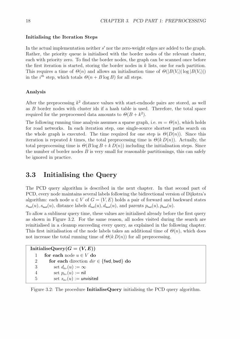
1 for each node u ∈ V do2 for each direction dir ∈ {fwd, bwd} do3 set ddir(u) := ∞4 set pdir(u) := nil5 set sdir(u) := unvisited
Figure 3.2: The procedure InitialiseQuery initialising the PCD query algorithm.

Chapter 4
PCD Part 2: Query
The PCD query algorithm presented in this chapter generally follows Dijkstra’s algo-rithm, which is introduced in Chapter 1, using the precomputed cluster distances in orderto visit a smaller number of nodes. Intuitively, the query is directed towards the target,so that only a small area around the shortest path is explored. In the section below, thebidirectional query algorithm of PCD is presented; the description of a unidirectionalvariant follows in Section 4.2.
4.1 The PCD Query Algorithm1
Input
Let G = (V, E) be a graph, w : E → IR≥0 a weight function, and s, t ∈ V the sourceand target node respectively. Furthermore, let V = {V1, . . . , Vk} be a partitioning of thegraph into k clusters with r(Vi) denoting the radius of a cluster Vi, d(Vi, Vj) the distancebetween two clusters Vi and Vj, and (sViVj
, tViVj) the corresponding startnode-endnode
pair. Moreover, let S, T ∈ V denote the clusters with s ∈ S and t ∈ T respectively.
Outline
The PCD query algorithm performs a bidirectional search from the source and thetarget node according to Dijkstra’s algorithm and comprises two phases. In both queryphases, forward and backward steps are performed repeatedly alternating between bothdirections. In each step, the node u with the smallest distance label is extracted froma priority queue Qdir corresponding to the current direction, the edges adjacent to u arerelaxed, and the shortest path distance from s to t is updated if necessary. The firstphase still follows Dijkstra’s algorithm exploring the source and target clusters untilborder nodes are found for both or the search directions meet.
Different from Dijkstra’s algorithm, PCD identifies nodes far away from the shortestpath during the second phase in order to prune them. This is done by maintaining an
1The figures in this chapter show the procedures relevant for the bidirectional version of the pruningalgorithm. The necessary changes for the unidirectional variant are also included.
19

20 CHAPTER 4. PCD PART 2: QUERY
PCD-Query(G=(V, E), w: E→ IR≥0, s, t ∈V, r: V → IR≥0, d: V×V → IR≥0)
1 InitialiseFirstPhase()
/ ∗ ∗ first query phase ∗ ∗ /
2 while ph-1fwd and ph-1bwd do3 extract minimum element u from Qdir
4 set sdir(u) := settled5 push u onto Stdir6 if sdir(u) = settled then7 CleanUpQuery()8 return9 for each edge e = (u, v) adjacent to u do
10 RelaxEdge(e)11 if sdir(v) = settled then set d := min (d, dfwd(v) + dbwd(v))12 if u is a border node then set ph-1dir := false13 if ph-1dir then set dir to dir14 InitialiseSecondPhase()
/ ∗ ∗ second query phase ∗ ∗ /
15 while Qfwd is not empty and Qbwd is not empty do16 extract minimum element u from Qdir
17 set sdir(u) := settled18 push u onto Stdir19 if sdir(u) = settled then20 CleanUpQuery()21 return
22 d(s, t):=UpdateUpperBound(u)23 d(s, u, t):=EstimateLowerBound(u)
24 if d(s, u, t) ≤ d(s, t) then25 for each edge e = (u, v) adjacent to u do26 RelaxEdge(e)27 if sdir(v) = settled then set d := min (d, dfwd(v) + dbwd(v))
28 set dir to dir
Figure 4.1: Bidirectional version of the PCD query algorithm. The procedures invokedcan be found in the succeeding figures, where in all the descriptions dir means theopposite of dir ; in other words, if dir = fwd then dir = bwd, and vice versa. Thedescription of the unidirectional version can be obtained by replacing line 28 with asuitable expression.

4.1. THE PCD QUERY ALGORITHM 21
RelaxEdge(e = (u, v))
1 set d′ := ddir(u) + w(e)2 if d′ < ddir(v) then3 set ddir(v) := d′
4 set pdir(v) := u5 if sdir(v) = unvisited then6 insert v into Qdir with priority ddir(v)7 set sdir(v) := visited8 else decrease priority of v in Qdir to ddir(v)
Figure 4.2: The procedure RelaxEdge is used in the uni- and bidirectional query.
upper bound of the total distance and estimating a lower bound whenever settling anode. If the lower exceeds the upper bound, the relevant node is not a member of theshortest path and will be pruned. The overall structure of the bidirectional algorithmcan be found in Figure 4.1, the relaxation procedure in Figure 4.2.
Variables
For every node u ∈ V , the PCD query algorithm maintains a forward and a back-ward state sfwd(u), sbwd(u) ∈ {unvisited, visited, settled}, as well as distance labels dfwd(u),dbwd(u) ∈ IR≥0 ∪ {∞} and parents pfwd(u), pbwd(u) ∈ V ∪ {nil}, similar to Dijkstra’s algo-rithm. Two min-priority queues Qfwd and Qbwd are maintained, again containing exactlythose nodes u ∈ V with sfwd(u) = visited and sbwd(u) = visited respectively. Additionally,if a node u contained in cluster Vi, i ∈ {V1, . . . , Vk}, is inserted into either priority queue,the cluster’s id i is stored with the node—this is necessary to identify cluster ids forinner nodes if a hash table for cluster ids of border nodes is used. When extracted fromeither priority queue, a node’s corresponding state will be set to settled. In additionto Dijkstra’s algorithm, an upper bound d(s, t) ∈ IR≥0 of the distance from s to t ismaintained, and the length d ∈ IR≥0 ∪ {∞} of the shortest path from s to t found sofar. The first border node of S found in the forward and the first of T found in thebackward search are denoted by s′ and t′, and two boolean variables ph-1fwd and ph-1bwd
indicate whether s′ and t′ have been found yet.
First Initialisation and Cleanup
In order to allow a sublinear execution time, the PCD query algorithm assumes theforward and backward states, distance labels, and parents of all nodes to be initialised.This initialisation is done at the end of the preprocessing part as shown in Figure 3.2of Chapter 3. For the same reason, the query is cleaned up after each search, usingtwo stacks St fwd and St bwd: initially empty, every node u extracted from Qdir during aquery is pushed onto the corresponding stack Stdir . When the query finishes, every nodeu on either stack Stdir is initialised for the next query by setting sdir(u) := unvisited,ddir(u) := ∞, and pdir(u) := nil. All nodes left in the priority queues Qfwd and Qbwd arereset in this way too. The whole cleanup procedure is summarised in Figure 4.3.

22 CHAPTER 4. PCD PART 2: QUERY
CleanUpQuery()
1 for each direction dir ∈ {fwd, bwd} do2 while Qdir is not empty do3 extract minimum element u from Qdir
4 set ddir(u) := ∞5 set pdir(u) := nil6 set sdir(u) := unvisited7 while Stdir is not empty do8 pop top element u from Stdir9 set ddir(u) := ∞
10 set pdir(u) := nil11 set sdir(u) := unvisited
Figure 4.3: The procedure CleanUpQuery initialising the next run of the PCD queryalgorithm.
InitialiseFirstPhase()
1 set sfwd(s) := visited2 set sbwd(t) := visited3 set dfwd(s) := 04 set dbwd(t) := 05 set pfwd(s) := nil6 set pbwd(t) := nil7 insert s into Qfwd with priority dfwd(s)8 insert t into Qbwd with priority dbwd(t)9 set ph-1fwd := true
10 set ph-1bwd := true11 set d := ∞12 set dir := fwd
Figure 4.4: The procedure InitialiseFirstPhase used in the bidirectional pruning al-gorithm.
Initialising the First Phase
Still, a constant amount of initialisation has to be done for each query, also shown inFigure 4.4: just like for Dijkstra’s algorithm, the forward state sfwd(s) of the startnode sis set to visited, the corresponding distance label sfwd(s) and parent pfwd(s) to zero and nilrespectively, and s is inserted into Qfwd with priority zero. The endnode t is processedanalogously for the backward direction, and the total distance value d is initialised with∞. Setting ph-1fwd := true and ph-1bwd := true, the query algorithms continues with thefirst phase.

4.1. THE PCD QUERY ALGORITHM 23
InitialiseSecondPhase()
1 set d(s, t) := 2 r(S) + d(S, T ) + 2 r(T )2 set dir to fwd
Figure 4.5: The procedure InitialiseSecondPhase initialises the upper bound of theshortest path length.
First Phase and Initialising the Second Phase
Every time a node is settled in this phase, a test whether it is a border node is performed.If a hash table for the border nodes is used, this can be done easily by a single lookup.If every node holds the id of its cluster, the test is to be performed during the relaxationby comparing the ids of both end points of each edge adjacent to the tested node. Thefirst phase finishes when border nodes of the source’s cluster S and the target’s clusterT have been visited, i.e. both ph-1fwd = false and ph-1bwd = false.
If the hash table for cluster ids is used, the cluster ids of S and T are not determinedup to this point. Therefore, nodes are inserted into Qfwd and Qbwd without any clusterinformation during the first phase. When such a node is extracted in the second phase, itwill be a member of S or T corresponding to the current direction. Inner nodes insertedin the second phase receive their cluster ids from their parent nodes.
The second phase is initialised by setting the upper bound of the total query distanced(s, t) := 2 r(S) + d(S, T ) + 2 r(T ) (see Figure 4.5). Since the ids of both S and T havebeen determined by the end of the first phase, looking up the values of r(S), d(S, T ),and r(T ) can actually be done. Note further that s′ and t′ have been determined bynow.
The following lemma shows the initial value of d(s, t) really is an upper bound of theshortest path distance from s to t.
Lemma 2 Let G = (V, E) be a weighted graph and V = {V1, . . . , Vk} a partitioning ofG into k clusters. For any nodes s, t ∈ V , the distance d(s, t) between s and t satisfies
d(s, t) ≤ 2 r(S) + d(S, T ) + 2 r(T ),
where S, T ∈ V are the clusters with s ∈ S and t ∈ T .
Proof: If S = T , then d(S, T ) = 0 and d(s, t) ≤ diam(S) ≤ 4 r(S). Otherwise, let p =(sST , . . . , tST ) be a shortest path from S to T , i.e. sST ∈ S, tST ∈ T , and w(p) = d(S, T ).Then, d(s, sST ) ≤ diam(S) ≤ 2 r(S) and d(tST , t) ≤ diam(T ) ≤ 2 r(T ), so there is a pathp′ = (s, . . . , sST , . . . , tST , . . . , t) from s to t with w(p) ≤ 2 r(S) + d(S, T ) + 2 r(T ). �
Second Phase: Updating the Upper Bound
After the upper bound has been initialised, it is repeatedly tried to be tightened in thesecond query phase as illustrated in Figure 1.5 of Chapter 1. In a forward step this

24 CHAPTER 4. PCD PART 2: QUERY
is potentially possible whenever a node u ∈ V with cluster id i ∈ {1, . . . , k} extractedfrom Qfwd is the first node sViT on the shortest path between Vi and T . Then, the valued′ := dfwd(u)+d(Vi, T )+dbwd(tViT ) is calculated if sbwd(tViT ) = settled. If tViT is not settledin the backward search, d′ can be estimated by dfwd(u)+d(Vi, T )+2 r(T ). If this is lowerthan the current value of the upper bound, then d(s, t) is decreased to d′. Figure 4.6summarises this update procedure and also contains the relevant expressions for thebackward direction, which is analogous. Another variant for updating the upper bound,which can be combined with the method above, is presented in Section 4.3 below.
Note that d(s, t) is not estimated in the latter way anymore as soon as all border nodesof S and T have been settled in the respective search direction. This holds particularlywhen sfwd(u) = settled for all u ∈ S and sbwd(u) = settled for all u ∈ T . The algorithm canbe thought of entering a third query phase at this point. This third phase is particularlyimportant for the unidirectional query algorithm as presented in Section 4.2 below.
UpdateUpperBound(u)
1 set d′ := ∞2 let U be the cluster containing u3 if dir = fwd then4 if u = sUT then5 if sbwd(tUT ) = settled then6 set d′ := dfwd(u) + d(U, T ) + dbwd(tUT )7 else8 set d′ := dfwd(u) + d(U, T ) + 2 r(T )9 else
10 if u = tSU then11 if sfwd(sSU) = settled then12 set d′ := dfwd(sSU) + d(S, U) + dbwd(u)13 else14 set d′ := 2 r(S) + d(S, U) + dbwd(u)
15 return min(d(s, t), d′)
Figure 4.6: The procedure UpdateUpperBound updating the upper bound of theshortest path distance. This procedure actually constitutes two pieces of codes in theactual implementation—one for each direction—avoiding the test in line 3, which isadded here for better readability. The unidirectional version is obtained by removinglines 9 to 14.
The value of d′ can be calculated easily: first, the test whether u is the first node on apath to T is done. Since the id i was stored with u in Qfwd, and the id of T is identifiedby the end of the first phase, sViT can be looked up (and compared to u) as well as tViT .Second, d(Vi, T ) and r(T ) can be obtained with these ids. Finally, dfwd(u) has just beenfound in the forward search, and dbwd(v) is only used if sbwd(v) = settled.
The following lemma shows that the values of d(s, t) obtained as described above do notexceed the distance between s and t.

4.1. THE PCD QUERY ALGORITHM 25
Lemma 3 Let G = (V, E) be a weighted graph and V = {V1, . . . , Vk} a partitioning ofG into k clusters. Then, for any pair of nodes s, t ∈ V and any cluster U ∈ V, thedistance d(s, t) between s and t satisfies the following four conditions:
d(s, t) ≤ d(s, sUT ) + d(U, T ) + d(tUT , t) (4.1)
d(s, t) ≤ d(s, sSU) + d(S, U) + d(tSU , t) (4.2)
d(s, t) ≤ d(s, sUT ) + d(U, T ) + 2 r(T ) (4.3)
d(s, t) ≤ 2 r(S) + d(S, U) + d(tSU , t), (4.4)
where S, T ∈ V with s ∈ S and t ∈ T , and sUT ∈ U, tUT ∈ T and sUS ∈ U, tUS ∈ S arethe startnode-endnode pairs of the shortest paths from U to T and U to S respectively.
Proof: s and t are connected by the two paths p1 = (s, . . . , sUT , . . . , tUT , . . . , t) andp2 = (s, . . . , sSU , . . . , tSU , . . . , t) with length values w(p1) = d(s, sUT )+d(U, T )+d(tUT , t)and w(p2) = d(s, sSU) + d(S, U) + d(tSU , t) respectively. Since d(s, t) ≤ w(p1) andd(s, t) ≤ w(p2), conditions 4.1 and 4.2 hold. Furthermore, d(tUT , t) ≤ diam(T ) ≤ 2 r(T )and also d(s, sSU) ≤ diam(S) ≤ 2 r(S), which proofs inequalities 4.3 and 4.4. �
Second Phase: Estimating Lower Bounds
After a possible update of the upper bound, a lower bound of the length of any pathfrom s to t containing u is calculated, where u ∈ V is the node just extracted and settled(see Figure 1.6). This lower bound d(s, u, t) is computed by dfwd(u) + d(U, T ) + dbwd(t
′)in a forward and dfwd(s
′) + d(S, U) + dbwd(u) in a backward step as shown in Figure 4.7.If this number is greater than the upper bound, the node u is not a member of theshortest path and can be pruned, which means the edges adjacent to u are not relaxed.Otherwise, relaxing is performed according to Dijkstra’s algorithm.
EstimateLowerBound(u)
1 let U be the cluster containing u2 if dir = fwd then3 return dfwd(u) + d(U, T ) + dbwd(t
′)4 else5 return dfwd(s
′) + d(S, U) + dbwd(u)
Figure 4.7: The procedure EstimateLowerBound calculates a lower bound of thedistance for paths from s to t containing node u. In the actual implementation, the testin line 2 is avoided since the procedure constitutes one separate piece of code for eachdirection. The figure merges both directions for better readability. Removing lines 4and 5 yields the suitable procedure for the unidirectional version of the query algorithm.
26 CHAPTER 4. PCD PART 2: QUERY
The expression for estimating d(s, u, t) is always defined: first, the distance value dfwd(u)or dbwd(u) is found in the corresponding direction as u has just been settled. Second, theid of U has been extracted together with u, and the ids of S and T are known by theend of the first phase, so d(S, U) and d(U, T ) can be looked up respectively. Last, s′ hasbeen determined and settled in the forward search and t′ in the backward search duringthe first phase, so the values of dfwd(s
′) and dbwd(t′) are defined.
The following lemma shows that this lower bound estimate holds. Only the statementfor the forward estimate is proved since the second estimate works analogously.
Lemma 4 Let G = (V, E) be a weighted graph and V = {V1, . . . , Vk} a partitioning ofG into k clusters. Then, for any three nodes s, u, t ∈ V , the weight w(p) of any pathp = (s, . . . , u, . . . , t) from s to t containing u satisfies the two conditions
w(p) ≥ d(s, u) + d(U, T ) + minv∈B(T )
d(v, t), if d(u, t) ≥ minv∈B(T )
d(v, t), and
w(p) ≥ minv∈B(S)
d(s, v) + d(S, U) + d(u, t), if d(s, u) ≥ minv∈B(S)
d(s, v),
where S, U, T ∈ V with s ∈ S, u ∈ U , and t ∈ T .
Proof: Let ps,u denote the subpath of p from s to u. Clearly, w(ps,u) ≥ d(s, u).
In the special case of u ∈ T , d(U, T ) = 0. Also, w(pu,t) ≥ d(u, t) holds, where pu,t is thesubpath of p from u to t, and so w(pu,t) ≥ min
v∈B(T )d(v, t) is satisfied by definition.
If u /∈ T , then there are nodes v′ /∈ T and t′ ∈ T such that p = (s, . . . , u, . . . , v′, t′, . . . , t).Then, the subpaths pu,t′ and pt′,t of p satisfy w(pu,t′) ≥ d(U, T ) and w(pt′,t) ≥ d(t′, t)respectively. Thus, also w(pt′,t) ≥ min
v∈B(T )d(v, t) since t′ is a border node of T . �
Total Distance, Shortest Path, and Stopping Condition
As mentioned before, a value d for the shortest path distance from s to t is maintainedduring the PCD query algorithm. This is updated when relaxing edges in either searchdirection: if an edge (u, v) has just been relaxed in direction dir , then sdir(u) = settled.If also sdir(v) = settled, a path from s to t of length ddir(v) + ddir(v) has been found, andthe value of d is decreased to this value if possible.
If the shortest path must be constructed after the search has finished, a meeting pointv ∈ V ∪ {nil} has to be maintained during the execution of the algorithm. Initialisedwith nil, it must be updated whenever d is updated, i.e. if d is set to dfwd(v) + dbwd(v)when relaxing an edge (u, v) ∈ E in either direction, v is set to v. Starting from v,the shortest path from s to t can then be reconstructed by successively following to theforward parent until s and to the backward parent until t is visited.
The query algorithm finishes if a node about to be settled in either direction is alreadysettled in the opposite direction.

4.1. THE PCD QUERY ALGORITHM 27
Correctness
The stopping condition above implicitly assumes that the search frontiers of both direc-tions eventually meet. It seems possible that the query algorithm keeps pruning nodeswithout inserting new nodes so that the priority queues run empty in the end. However,this will not happen. The main argument is that nodes on the shortest path are neverpruned as shown in Lemma 5. Note that any node settled in either search directionwill not be considered for pruning in the opposite direction according to the stoppingcondition above.
Lemma 5 Let G = (V, E) be a weighted graph and V = {V1, . . . , Vk} a partitioning ofG into k clusters. The PCD query algorithm never prunes a node on the shortest pathfrom s to t for any query with source s ∈ V and target t ∈ V .
Proof: Let SP = (s, . . . , t) be the shortest path from s to t and let u ∈ V be any nodeof this path. Further, let S, T ∈ V be the pair of clusters with s ∈ S and t ∈ T .
If d(u, t) ≤ minv∈B(T )
d(v, t), u will be settled in the backward direction already in the first
phase, where no pruning happens at all; further, it will not be considered for pruning inthe opposite direction during the second phase. By the analogous argument, u will notbe pruned if d(s, u) ≤ min
v∈B(S)d(s, v) either.
Now assume that d(s, u) > minv∈B(S)
d(s, v) and d(u, t) > minv∈B(T )
d(v, t). As w(SP) = d(s, t),
d(s, t) ≥ d(s, u, t) is satisfied by Lemma 4. On the other hand, d(s, t) ≤ d(s, t) at anytime of the query by Lemma 2 and Lemma 3. Therefore, d(s, u, t) ≤ d(s, t) whenever uis considered for pruning. �
As mentioned above, the immediate consequence from this is that the PCD query algo-rithm never runs dry, which is shown in Theorem 1. Nodes will be available for settlinguntil the search frontiers meet, and the stopping condition eventually applies. Besides,the looping condition of the second phase, shown in line 15 of Figure 4.1, is alwayssatisfied and can be replaced by ’true’.
Theorem 1 For any pair of source s and target t, both priority queues Qfwd and Qbwd
contain at least one node of the shortest path from s to t until the search frontiers meet.
Proof: The statement is proven for Qfwd by induction: let SP denote the shortest pathfrom s to t. The source s ∈ SP is inserted into Qfwd at initialisation, so the assumptionholds when the algorithm starts. Then, whenever a node u ∈ SP is extracted from Qfwd,it will not be pruned by Lemma 5. Therefore, u’s successor on SP is inserted into Qfwd
if it is not contained yet, and Qfwd still holds a member of SP. The proof for Qbwd isanalogous. �
The path found when finishing not only is a valid path from the source to the target,it also is the shortest. This fact is shown in the following theorem which completes thecorrectness of the PCD query algorithm.

28 CHAPTER 4. PCD PART 2: QUERY
Theorem 2 For a query from any source s to any target t, the distance d found by thePCD query algorithm upon finishing satisfies d = d(s, t).
Proof: Assume w.l.o.g. that the algorithm stops in a forward step with settling a nodex ∈ V , which means both sfwd(x) = settled and sbwd(x) = settled.
If x /∈ SP , there is a node v ∈ SP contained in Qfwd by Theorem 1, and so their forwarddistance labels satisfy dfwd(x) ≤ dfwd(v). Let u ∈ SP be the predecessor of v on theshortest path and assume w.l.o.g. that sfwd(u) = settled. Then, dbwd(v) < dbwd(x) sinceotherwise x would be a member of SP. This implies sbwd(v) = settled, which togetherwith sfwd(u) = settled implies that the four distance labels of u and v hold the distancesfrom s and to t. Now, d contains the value dfwd(u) + dbwd(u) if u was settled before v.Otherwise, d = dfwd(v) + dbwd(v).
If x ∈ SP , let x′ ∈ SP be the predecessor of x on the shortest path. x′ is settled inthe forward direction since d(s, x′) < d(s, x). If this settling happened before x wassettled in the backward direction, then d carries the value dfwd(x
′) + dbwd(x′). Otherwise,
d = dfwd(x) + dbwd(x). �
4.2 The Unidirectional Version
In the following, the unidirectional PCD pruning algorithm is outlined. Also this variantbasically follows Dijkstra’s algorithm and can be derived easily from the bidirectionalquery described in the preceding section. The figures shown there contain the informa-tion how to receive the relevant descriptions of the unidirectional procedures.
The unidirectional PCD query algorithm maintains the same set of variables and isgiven the same input, so the uni- and bidirectional versions use the same preprocessing.Initialisation, cleanup, and the first phase exactly remain unchanged, while pruning isonly performed by the forward search of the second phase. The backward search justfollows Dijkstra’s algorithm not estimating any upper or lower bounds.
However, only few steps in the backward direction are performed. The backward searchis cancelled as soon as sbwd(u) = settled for all nodes u in the target cluster T . Then, thedistance from every node u ∈ T to the target t is contained in u’s backward distance labeldbwd(u); in particular, the distance from every border node u ∈ B(T ) of T to the targett has been found. As mentioned in the section above, the algorithm can be thought ofas entering a third query phase since the values of dbwd(tUT ), as used in Figure 4.6, donot need to be approximated by the diameter diam(T ) of T anymore. For this reason,line 28 of Figure 4.1, which alternates between the directions, must be replaced in theunidirectional algorithm by the following expression:
28a if sbwd(u) = settled for all u ∈ T then28b set dir := fwd28c else
28d set dir := dir

4.3. UPPER BOUNDS AT CLUSTER ENTRY 29
This expression is avoided in the actual implementation where the third phase comprisesan independent piece of code only containing a forward direction. Also, only one expres-sion updating the upper bound is used for this third phase avoiding the test in line 5 ofFigure 4.6. Still, the test has to be done a few times to determine the end of the secondphase and can be accomplished easily if the sizes of the clusters are given as a furtherinput.
The way of updating the value of d as well as the stopping condition remain unchangedcompared to the bidirectional pruning algorithm. The search will usually finish in aforward step since the backward search roughly explores only the target cluster andsome surrounding area. Again, a meeting point can be maintained along with the totaldistance if the shortest path is to be constructed.
The only purpose of searching from the target is to determine the distances between theborder nodes of the target cluster and the target, So the unidirectional query algorithmcan also be thought of an asymmetric bidirectional search. The term ’asymmetric’reflects that one direction is cancelled early, whereas a full backward search is performedin the bidirectional algorithm.
4.3 Upper Bounds at Cluster Entry
Motivation
As explained in the previous sections, the PCD query algorithm repeatedly tries toupdate the upper bound of the shortest path distance. In the forward search, thishappens whenever a startnode of a precomputed shortest path to the target clusteris settled. Intuitively, this situation occurs when a cluster is left by the search to thedirection of the target cluster and a new cluster is about to be entered. This considerationmotivates using some information of a new cluster already when it is entered instead ofwaiting until the startnode of the shortest path from this to the target cluster is found.
Method
The following variant for updating the upper bound tries to exploit this thought. Letu ∈ V be a node contained in cluster U ∈ V and extracted from Qfwd in a forward step.Then, if u is the first of all nodes of U settled in this direction, the value
d′ := dfwd(u) + 2 r(U) + d(U, T ) + dbwd(tUT ) (4.5)
is calculated if sbwd(tUT ) = settled. If tUT has not been settled in the backward searchyet, d′ can be estimated with
dfwd(u) + 2 r(U) + d(U, T ) + 2 r(T ). (4.6)
For the corresponding situation in the backward search—only relevant for the bidi-rectional query algorithm—the appropriate expressions are d′ := dfwd(sSU) + d(S, U) +2 r(U)+dbwd(u) if sfwd(sSU) = settled and d′ := 2 r(S)+d(S, U)+2 r(U)+dbwd(u) otherwise.As before, the upper bound is decreased to this estimate if d′ < d(s, t).

30 CHAPTER 4. PCD PART 2: QUERY
These values for d′ can be calculated easily: u has just been settled, so dfwd(u) is deter-mined and r(U) can be looked up as U ’s id has been extracted with u. Also, T ’s clusterid as well as tUT are known since the first query phase has been finished, so lookingup d(U, T ) and testing sbwd(tUT ) are both possible. Furthermore, r(T ) can be lookedup with T ’s cluster id. Similar arguments hold for the two analogous backward terms.Moreover, a label indicating whether U has been entered yet must be maintained forevery cluster U ∈ V .
Correctness
It is easy to see that all the four different estimates from above actually are upper boundsof d(s, t). Obviously, there is a shortest path from u ∈ U to sUT ∈ U whose length is atmost 2 r(U). The distance between sUT and tUT is d(U, T ). Thus, there is a path from sto t containing u, sUT , and tUT with a length of at most d(s, u)+r(U)+d(U, T )+d(tUT , t),so the term in 4.5 is an upper bound of d(s, t). The same holds for the expression inequation 4.6 since d(tUT , t) ≤ 2 r(T ) holds, as tUT ∈ T and t ∈ T . Both the estimatesfor the backward direction hold for similar arguments.
Note that any node v ∈ U settled later than u ∈ U satisfies dfwd(v) ≥ dfwd(u), so only thefirst node of a cluster is worth considering.
Results
Updating the upper bound as described in Section 4.1 performs much better than thisvariant. Though the latter causes many updates at an early stage of the search, thefinal upper bound is much tighter when using the former method. Both variants can becombined easily, but this does not improve the measured speedups compared to usingthe first variant exclusively.

Chapter 5
PCD Part 0: Partitioning
In this chapter several ways of graph partitioning are presented, any of which can be usedto provide a clustering for the PCD algorithm. The notion of a k-center clustering isintroduced first; then, grid clustering and METIS are presented, providing two well-knownpartitioning methods as a basis for comparison. Although PCD works independentlyof the clustering method, the actual partitioning has a strong influence on the queryperformance, which is analysed in Chapter 6. Throughout this chapter the effect ofthe partitioning method on the cluster sizes and diameters is mentioned repeatedly,measured data for which can be found in Figures 6.7–6.9.
5.1 k-Center Clustering
As mentioned in Section 2.4, the idea of the k-center problem implicitly provides amethod of graph partitioning. This is presented in the following, including different waysto obtain clusterings of this kind and to adjust their major characteristics concerningthe influence on the query performance.
5.1.1 Basics
Definition
Let G = (V, E) be a graph and w : E → IR≥0 be a weight function. Furthermore, letC = {c1, . . . , ck} ⊆ V be a set of k distinct nodes called the center nodes. Then, asubdivision V = {V1, . . . , Vk} of pairwise disjoint sets Vi ⊆ V , 1 ≤ i ≤ k, is called ak-center clustering if both the following conditions hold:
•k⋃
i=1
Vi = V .
• For every u ∈ V and 1 ≤ i ≤ k: if u ∈ Vi, then d(u, ci) ≤ d(u, cj) for every1 ≤ j ≤ k.
Note that a k-center clustering for a given graph and a set of center nodes is not uniquesince a (non-center) node might have the same distance to different centers.
31

32 CHAPTER 5. PCD PART 0: PARTITIONING
In connection with a k-center clustering, the radius r(Vi) of a cluster Vi will alwaysrefer to the maximum of the distances between any member of Vi and its center. Notethat 2 r(Vi) is an upper bound of the cluster’s diameter: let G = (V, E) be a weightedgraph and c ∈ V be the center node of a cluster U ∈ V in a k-center clustering Vof G. Furthermore, let u, v, w ∈ U be members of this cluster such that its radius isdefined by u, i.e. r(U) = d(u, c), and the diameter satisfies diam(U) = d(v, w). Then,diam(U) = d(v, w) ≤ d(v, c) + d(c, w) ≤ 2 d(u, c) = 2 r(U). This fact is used in thequery to initialise the upper bound as shown in Chapter 4 above.
Computation
Given a graph G = (V, E) and a set C = {c1, . . . , ck} ⊆ V of k center nodes, a k-centerclustering can be calculated by one single source shortest path search in the followingway: first, a dummy node s′ is inserted and connected to each center node by a zero-weight edge, and a single source shortest path search is started from s′. For every nodeu ∈ V , a node label c(u) is maintained containing the center a node is currently assignedto. Initialised with c(ci) = ci for every center ci ∈ C, these node labels are then updatedwhenever the predecessor of a node changes. Finally, if a node u ∈ V is settled andc(U) = ci, u is assigned to cluster Vi.
Every node is assigned to exactly one cluster, so the clusters are disjoint and their unionadds up to V , while the second condition in the definition in Section 5.1.1 is satisfied bythe following lemma:
Lemma 6 d(s′, u) = min1≤i≤k
d(ci, u) for every node u ∈ V .
Proof: Let u ∈ V and SP = (s′, cj, . . . , u), 1 ≤ j ≤ k, be the shortest path from s′ tou. If p = (ci, . . . , u) is any path from any ci, 1 ≤ i ≤ k, to u and p′ = (s′, ci, . . . , u) thecorresponding extension, then w(p) = w(p′). Thus, d(s′, u) = w(SP) ≤ w(p′) = w(p). �
This process takes time Θ(D(n)). Moreover, the values of the sizes and the radii of theclusters can be estimated during this search without affecting the asymptotic calculationtime: initialised with zero, the size of a cluster is incremented when a node is finallyassigned to it, while its radius is updated to the distance label of this node at the sametime. Note that the radii of the clusters do not decrease during the search.
Directed Graphs
The definition above generally applies to directed graphs too, assigning a node u to thecenter node closest from u, while assigning to the center c with the smallest distancefrom c to u is also possible. However, in order to preserve the relation between the clusterradius and diameter, the second condition of the definition above must be changed to:
• For every u ∈ V and 1 ≤ i ≤ k: if u ∈ Ci, then max (d(u, ci), d(ci, u)) ≤max (d(u, cj), d(cj, u)) for every 1 ≤ j ≤ k.

5.1. K-CENTER CLUSTERING 33
The radius r(Vi) of a cluster Vi can then be defined by r(Vi) = minu∈Vi
max (d(u, ci), d(ci, u))
and still satisfies diam(Vi) ≤ 2 r(Vi): let u, v, w ∈ Vi be members of a cluster Vi ∈ Vsuch that its radius is defined by u, i.e. r(Vi) = max (d(u, ci), d(ci, u)), and its diameterdiam(Vi) is given by diam(Vi) = d(v, w). Then, diam(Vi) = d(v, w) ≤ d(v, ci)+d(ci, w) ≤2 max (d(u, ci), d(ci, u)) = 2 r(U).
Choosing the Center Nodes
The way of partitioning has an influence on the shape of the clusters, which againaffects the query performance of PCD. So, since the set of centers determines a k-centerclustering, its choice has a strong effect on the PCD query algorithm.
A straight-forward way is choosing the center nodes randomly. This results in a k-centerclustering with quite uniform sizes but unequal diameters, and the query performanceof this is not even bad (see Section 6.3.2). However, this can be improved as shown inthe following.
5.1.2 k′-Oversampling
An intuitive way to improve a clustering is to remove centers that determine clusterswith adverse characteristics. For this reason, some more centers can be chosen initiallyin order to remove the worst of them until the desired number of clusters is left.
Algorithm
Given a weighted graph G = (V, E) and a positive integer k, a k-center clustering for Gcan be obtained by the method of k′-oversampling : a sample set C ′ of k′ centers is chosenrandomly from the set of nodes V for some k′ ≥ k, and a k′-clustering is computed for it.Then, clusters are deleted successively by removing their centers from C ′ until exactlyk clusters are left.
The initial k′-clustering is computed in the way described in Section 5.1, while deletinga cluster and possible heuristics for selecting it are described below.
Deleting a Cluster
When removing a node ci from the set C ′ of k′ centers, the resulting (k′−1)-clusteringdoes not need to be recomputed completely. Since removing ci does not affect any nodeu ∈ V outside Vi, only the members of Vi need reassigning to the remaining centers.
As illustrated in Figure 5.1, this is done in the following way: first, a breadth first searchis performed starting from ci in order to find all the neighbour nodes of Vi. Then, adummy node s′ is introduced and connected to each of these neighbours v ∈ Vj, i 6= j, byone edge (s′, v) of weight d(v, cj), where cj denotes the center of Vj. Running a shortestpath search from s′ on the graph consisting of s′, the members and neighbours of Vi,the dummy edges, and the maximal subset of E, all nodes u ∈ Vi are then assigned to
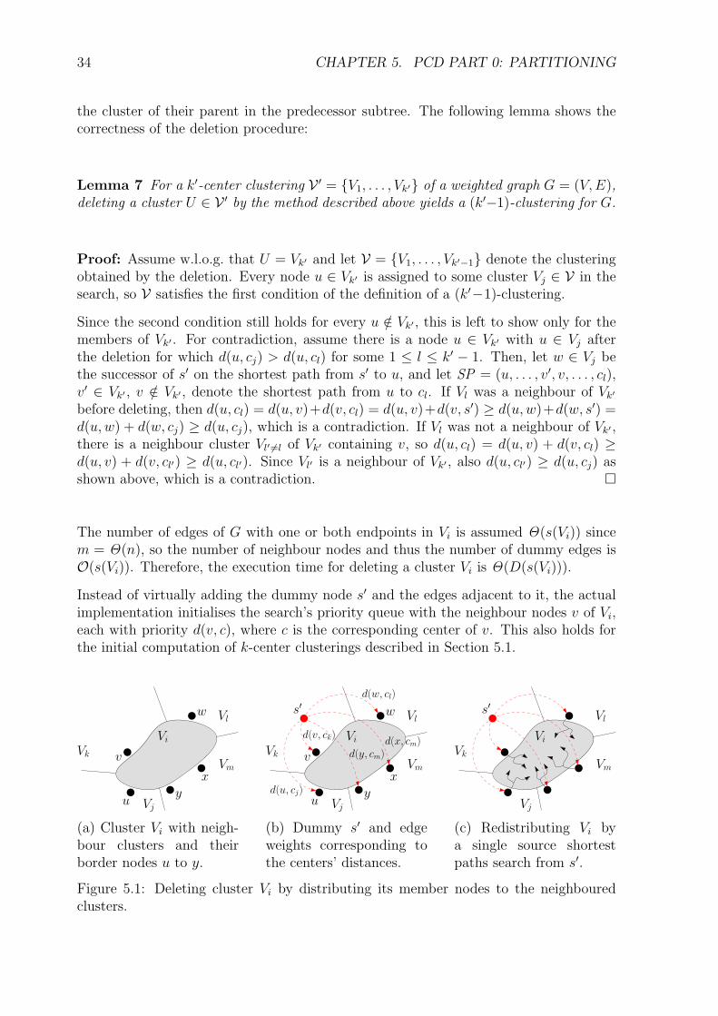
34 CHAPTER 5. PCD PART 0: PARTITIONING
the cluster of their parent in the predecessor subtree. The following lemma shows thecorrectness of the deletion procedure:
Lemma 7 For a k′-center clustering V ′ = {V1, . . . , Vk′} of a weighted graph G = (V, E),deleting a cluster U ∈ V ′ by the method described above yields a (k′−1)-clustering for G.
Proof: Assume w.l.o.g. that U = Vk′ and let V = {V1, . . . , Vk′−1} denote the clusteringobtained by the deletion. Every node u ∈ Vk′ is assigned to some cluster Vj ∈ V in thesearch, so V satisfies the first condition of the definition of a (k′−1)-clustering.
Since the second condition still holds for every u /∈ Vk′ , this is left to show only for themembers of Vk′ . For contradiction, assume there is a node u ∈ Vk′ with u ∈ Vj afterthe deletion for which d(u, cj) > d(u, cl) for some 1 ≤ l ≤ k′ − 1. Then, let w ∈ Vj bethe successor of s′ on the shortest path from s′ to u, and let SP = (u, . . . , v′, v, . . . , cl),v′ ∈ Vk′ , v /∈ Vk′ , denote the shortest path from u to cl. If Vl was a neighbour of Vk′
before deleting, then d(u, cl) = d(u, v)+d(v, cl) = d(u, v)+d(v, s′) ≥ d(u, w)+d(w, s′) =d(u, w) + d(w, cj) ≥ d(u, cj), which is a contradiction. If Vl was not a neighbour of Vk′ ,there is a neighbour cluster Vl′ 6=l of Vk′ containing v, so d(u, cl) = d(u, v) + d(v, cl) ≥d(u, v) + d(v, cl′) ≥ d(u, cl′). Since Vl′ is a neighbour of Vk′ , also d(u, cl′) ≥ d(u, cj) asshown above, which is a contradiction. �
The number of edges of G with one or both endpoints in Vi is assumed Θ(s(Vi)) sincem = Θ(n), so the number of neighbour nodes and thus the number of dummy edges isO(s(Vi)). Therefore, the execution time for deleting a cluster Vi is Θ(D(s(Vi))).
Instead of virtually adding the dummy node s′ and the edges adjacent to it, the actualimplementation initialises the search’s priority queue with the neighbour nodes v of Vi,each with priority d(v, c), where c is the corresponding center of v. This also holds forthe initial computation of k-center clusterings described in Section 5.1.
Vi
Vj
Vk
Vl
Vmx
yu
v
w
(a) Cluster Vi with neigh-bour clusters and theirborder nodes u to y.
s′
Vi
Vj
Vk
Vl
Vm
d(w, cl)
d(y, cm)
d(v, ck)
d(u, cj)
d(x, cm)
x
yu
v
w
(b) Dummy s′ and edgeweights corresponding tothe centers’ distances.
s′
Vi
Vj
Vk
Vl
Vm
(c) Redistributing Vi bya single source shortestpaths search from s′.
Figure 5.1: Deleting cluster Vi by distributing its member nodes to the neighbouredclusters.
5.1. K-CENTER CLUSTERING 35
Choosing a Cluster for Deletion
The question remains how to select a center and thus a cluster in a deletion step ofk′-oversampling, which is important since this finally decides the characteristics of theresulting k-center clustering: the lower the diameter of a cluster is, the better the lowerbounds for its member nodes are, and small clusters are crossed more quickly causingmore frequent updates of the upper bound. Therefore, an optimal partitioning hasclusters of even size and low diameter. Road networks usually have a non-uniformstructure with highly differing edge weights between urban and rural regions, whichmakes it difficult to achieve such a clustering.
For a high value of k′ compared to k, the initial k′-center clustering has clusters of verylow sizes and diameters, while deleting a cluster increases the sizes and diameters ofits neighbours. This increase is to be confined, which motivates the following deletionheuristics:
• MinSize: The minimum size heuristic selects the smallest cluster in terms ofnumber of nodes. This rule aims for limiting the remaining clusters growing insize.
• MinRad: The minimum radius heuristic selects the cluster with the currentlysmallest radius. This rule aims for restricting the neighbour clusters’ diameters.
• MinSizeRad: The minimum size/radius heuristic alternates between MinSize andMinRad in consecutive steps. This rule tries to control both sizes and diametersof the remaining clusters.
The way of redistributing a deleted cluster causes neighbours with a bigger radius to growless, which yields fairly low average diameters independently of the heuristic. However,the average speedups of the PCD query algorithm vary for different deletion heuristics,which is explained in Section 6.3.2 in more detail.
Analysis
As shown in Section 5.1, calculating the initial k′-center clustering affords a time ofD(n), independently of the number k′, while deleting a cluster Vi takes D(s(Vi)).
The cluster size is bounded by s(Vi) ≤ n−k′+i = O(n), where i ∈ {1, . . . , k′−k} denotesthe number of the current deletion step. Therefore, the execution time of calculating ak-center clustering by k′-oversampling amounts to O((k′ − k) D(n)) in the worst case,which is O(k log k D(n)) if putting k′ = k log k.
If the MinSize heuristic is used, the cluster size can be bounded by s(Vi) ≤ nk′−(i−1)
in the
ith step, i ∈ {1, . . . , k′ − k}. By the following consideration, this allows improving therunning time to O
(n log n log k′
k
), which furthermore becomes O(n log n log log k) when
putting k′ = k log k, assuming a running time of D(n) = O(n log n) for a single sourceshortest paths search:

36 CHAPTER 5. PCD PART 0: PARTITIONING
O
(k′∑
i=k+1
D(n
i
))= O
(k′∑
i=k+1
n
ilog
n
i
)
= O
k′∑
i=k+1
n
ilog n−
k′∑i=k+1
n
ilog i︸ ︷︷ ︸
≥0
= O
(n log n
(k′∑
i=1
1
i−
k∑i=1
1
i
))= O (n log n (log k′ − log k))
= O(
n log n logk′
k
)The actual partitioning times measured for the several deletion heuristics are comparedto each other in Section 6.3.2.
5.1.3 Local Search
The method of oversampling starts with a clustering of more than k clusters in orderto delete some of them. Instead, it is possible to start of with a k-center clustering andreplace adverse clusters with better ones by repeatedly deleting a center and insertinganother.
Algorithm
Given a weighted graph G = (V, E) and a positive integer k, a k-center clusteringV = {V1, . . . , Vk} is assumed to have been computed, whose corresponding set of centernodes is denoted by C. In each step of the algorithm, one cluster is deleted by removingits center from C, and one cluster is inserted instead by adding a new center to C. Thisstep is performed repeatedly.
The initial k-center clustering can be obtained by randomly choosing of center nodesas described in Section 5.1 for example, but also a k-center clustering computed withk′-oversampling can be refined by local search. Clusters are chosen an deleted exactly asdescribed in Section 5.1.2, while inserting, where to insert it, and aborting are describedin the following.
Inserting a Cluster
When a new center node c is added to C, it is not necessary to completely recomputethe resulting clustering since only few nodes around the new center need reassigning.For this reason, a shortest path search is started from c. In this search, a node u ∈ Vi
5.1. K-CENTER CLUSTERING 37
is inserted into the priority queue only if its distance label is smaller than d(u, ci), i.e.the distance to its current center. Each time a node is settled, it is assigned to the newcluster, and the search finishes when the priority queue is empty.
Deleting a cluster was proven to work correctly in Section 5.1.2. Combined with thefollowing lemma, this yields the k-center clustering conditions are preserved in everystep of the algorithm. W.l.o.g. Vk is assumed to be the cluster inserted.
Lemma 8 For every node u ∈ V , u ∈ Vk iff d(u, ck) < d(u, cj) for every 1 ≤ j ≤ k− 1.
Proof: If u ∈ Vk, then u was settled once during the cluster insertion procedure. Thus,u had been inserted into the priority queue before, so d(u) < d(u, cj) must have held atthat time, where cj denotes u’s former center, and d(u, ck) ≤ d(u) since u’s priority canonly decrease afterwards. Further, d(u, cj) < d(u, ci) for 1 ≤ i ≤ k−1 as the (k−1)-centerproperties are satisfied prior to inserting the cluster. Therefore, d(u, ck) < d(u, cj) forevery 1 ≤ j ≤ k − 1.
Conversely, if u /∈ Vk, this has also held before inserting the cluster Vk. Then, letp = (u, . . . , v, v′, . . . , ck), v ∈ Vl 6=k, v′ ∈ Vk, be the shortest path from u to ck. When v′
was settled, v was not inserted into the queue, so d(v, cl) ≤ d(ck, v′)+w((v′, v)) = d(ck, v)
is satisfied. Thus, d(u, ck) = d(u, v) + d(v, ck) ≥ d(u, v) + d(v, cl) ≥ d(u, cl). �
Choosing a New Center
The node added to the set of centers determines the resulting k-center clustering andmust therefore be chosen carefully. This selection can be used to reduce the size ordiameter of other clusters, which motivates the following selection strategies:
• MaxRad: The maximum radius strategy chooses the node with the highest dis-tance to its center, which is equal to the maximum radius of all clusters, and aimsfor reducing the cluster diameters.
• MaxSize: The maximum size strategy chooses the node with the highest distanceto the center from the largest size cluster, aiming for uniform size clusters byreducing the size of the largest.
To follow either of these strategies, a priority queue has to be maintained, whose min-imum item contains the next node for insertion. Furthermore, either approach can becombined with any deletion strategy described in Section 5.1.2.
Stopping
It is possible to fix the number of iterations before starting the local search, for exampleby a function depending on the number of clusters k. However, it seems more reasonableto stop the algorithm as soon as a certain clustering characteristic does not improve anyfurther, such as the average cluster radius or the maximum cluster size.

38 CHAPTER 5. PCD PART 0: PARTITIONING
Results
Some first experiments are conducted using local search in order to improve k-centerclusterings obtained by k′-oversampling. Unfortunately, the algorithm started choosingthe same centers for insertion and deletion repeatedly already after few iterations, par-ticularly for the MinSize deletion heuristic which yields the best speedups as shown inSection 6.3.2. However, other selection rules for inserting and deleting might help onthis, as well as more sophisticated combinations of them and also removing a highernumber of clusters before inserting the same number again. Furthermore, some de-gree of randomness, such as inserting the furthest node of a randomly selected cluster,seems suitable to escape from a looping situation. All this suggests there still is a lot ofpotential in the idea of improving k-center clustering by local search.
Moving Center Nodes
Since the centers of two neighboured clusters might have a low distance, moving sucha center node towards the central point of its cluster can yield a better radius withoutchanging the clustering too much.
Generally, moving a center node of a k-center clustering can be viewed as deleting acluster and inserting a new one, where the position of the inserted center is determinedprevious to the deletion.
5.2 Grid Clustering
A quite simple approach of graph partitioning is to arrange a clustering in a grid-likemanner: a square grid is applied above the graph, and all nodes in the same squaretogether form a cluster. This method needs node coordinates, and the graph instancesused for testing indeed contain this information. However, this is the only point wherethey are used.
To achieve a grid clustering with (at least) k clusters, the side length l of a square hasto be chosen carefully. W.l.o.g. let xmin = 0, xmax = 1, ymin = 0, and ymax = c be theminimum and maximum x- and y-coordinates respectively of all nodes in a given graph.Now, put the side length l =
√ck, the number of squares in the horizontal direction
a =⌈
1l
⌉, and the number of squares in the vertical direction b =
⌈al
⌉. With this choice
all nodes will be covered since a l ≥ 1 and b l ≥ c, and sufficiently many clusters will beachieved since a b ≥ k. Note that empty squares might occur, which would yield emptyclusters and thus can be deleted.
For a graph with n nodes featuring geographic coordinates, a grid clustering can becalculated in time Θ(n). Obtaining the radii of the clusters is described in Section 5.4below.

5.3. METIS 39
5.3 METIS
An approach much more sophisticated than grid clustering is provided by the softwarepackage METIS [Met95], which is originally intended for balancing computations in par-allel processing while minimising the communication volume. It contains a variety ofprograms and libraries for partitioning graphs, particularly procedures for calculatingk-way partitionings. A k-way partitioning of a graph G = (V, E) is a partitioning V ofk clusters according to the definition in Section 2.3 with the additional property that|U | = n
kfor every partition U ∈ V. The relevant METIS procedure follows a multilevel
k-way partitioning scheme described in [KK98], and finds a clustering of k equal sizeregions (not necessarily contiguous), minimising the edge cut, where the edge cut of apartitioning denotes the number of edges with end nodes in different clusters. Also forclusterings computed with METIS, the cluster radii must be estimated in a postprocessingstep described in the following section.
The clusters obtained by METIS are of perfectly uniform size. On the other hand, thisis paid for with highly differing diameters, which is further added to by possible non-contiguous clusters. The resulting effects on the query are examined in Section 6.3.2.
5.4 Cluster Radii
In the PCD query algorithm, a value for the radius of every cluster is used for initialisingand estimating the upper and lower bounds. While radii are obtained along the waywhen oversampling, they must be estimated separately for grid clustering and METIS.
This is done for each cluster U ∈ V of a partitioning V in the following way: a randomnode u ∈ U is selected, and the node v ∈ U furthest away from u is determined by ashortest path search. Then, the node w ∈ U furthest away from v is estimated in thesame way. Finally, the node c in the middle of the shortest path from v to w is chosento be the center of this cluster, and the furthest shortest path distance from c inside Uas the radius. If c is not a member of U—which can happen since clusters obtained byMETIS or grid clustering may not be connected—the member node of U on the shortestpath closest to c is chosen.
This step must be performed once for each cluster resulting in a total time of O(k D(n))in the worst case for a partitioning of k clusters.
For any partitioning V = {V1, . . . , Vk}, an upper bound of the diameter diamVi is ob-tained for each cluster U ∈ V in this way. This is easy to see: let U ∈ V be any clusterwith center c ∈ U . Then, any pair of nodes u, v ∈ U satisfies d(u, v) ≤ d(u, c)+d(c, v) ≤2 r(U), and therefore diam(U) ≤ 2 r(U). The quality of the radius, i.e. the differencebetween the diameter and two times the radius, varies for the different clustering meth-ods. Since most clusters obtained with METIS show a ‘round’ shape, their radius is notmuch bigger than half the diameter, while partitions in a k-center clustering may bemore ‘longish’. Disconnected clusters in METIS or grid have a high diameter (and also ahigh radius), but this does not affect the average query if only few nodes lie outside thelargest connected portion. This consideration has to be kept in mind with regard to theanalysis in Section 6.3.2, in which the different partitionig methods are compared.

Chapter 6
Experiments
6.1 Test Instances
All test instances used for the experiments presented in Section 6.3 represent real-worldroad networks, whose names and sizes can be found in Table 6.1 for the Europeanand Table 6.2 for the US road network. For every instance, two different edge weightfunctions are available, one corresponding to average travel times, the other to traveldistances.
The graphs listed in Table 6.1 represent the road network of the 14 Western Europeanstates of Austria, Belgium, Denmark, France, Germany, Italy, Luxembourg, the Nether-lands, Norway, Portugal, Spain, Sweden, Switzerland, and Great Britain. The originaldata for this—which was made available for scientific use by PTV AG—contains onelength value for each edge, which provides the distance function. Furthermore, eachedge is assigned one out of 13 road categories, ranging from forest roads to fast mo-torways. To each category, an average travel speed between 10 km/h and 130 km/h isassigned, which yields the average travel time of each edge. Furthermore, some edgesrepresent ferry connections for which the average travel times are contained in the inputdata. The graphs DEU and SUI are subgraphs of CEN and WSO respectively.
The graphs listed in Table 6.2 represent the road network of the 48 contiguous states ofthe United States and the District of Columbia, which was obtained from [U.S02]. The
Instance n m Description
CEN 5,342,276 6,664,561 Belgium, Danmark, Germany,Luxembourg, the Netherlands
WSO 4,190,068 5,251,527 Austria, France, Switzerland, ItalySCA 2,453,610 2,731,129 Norway, SwedenGBR 2,149,793 2,590,401 Great BritainIBE 872,083 1,177,734 Spain, Portugal
DEU 4,375,849 5,483,579 GermanySUI 630,962 771,694 Switzerland
Table 6.1: The graph instances of the European road network used for the experiments.
40

6.2. EXPERIMENTAL SETUP 41
Instance n m Description
SOU 7,588,996 8,851,170 South (AL, AR, FL, GA, KY, LA, MS, MO, NC,SC, TN, VA, WV)
MID 5,246,822 6,494,670 Midwest (IL, IN, IA, KS, MI, MN, NE, ND, OH,SD, WI)
WES 4,429,488 5,296,150 West (CA, CO, ID, MT, NV, OR, UT, WA, WY)SWT 3,561,925 4,382,697 Southwest (AZ, NM, OK, TX)MAT 2,226,138 2,771,948 Middle Atlantic (DC, DE, MD, NJ, NY, PA)NEN 896,115 1,058,481 New England (CT, ME, MA, NH, RI, VT)
Table 6.2: The graph instances of the US road network used for the experiments.
original data also contains a road category for each edge as well as a length value, fromwhich an average travel time is determined in the same way as above. However, thereare only four different categories ranging from local roads to primary highways, to whichaverage speeds between 40 km/h and 100 km/h are assigned.
All instances are undirected, connected, and do not have any self-loops or paralleledges. As mentioned before, undirected graphs are only used for the sake of simplerpartitioning—the precomputing and query algorithms work for directed graphs too. Theinformation about the direction of each edge in the original data for the European in-stances is ignored, whereas no direction is available for the US instances. Furthermore,the original data provides geographic coordinates for each node; this information is onlyused for estimating the grid clustering described in Section 5.2. The instances used aregenerated in the same way as in [Sch05], in particular, the same average speeds areassigned to the road categories when deriving the travel times.
The graphs reflect the following characteristic of the real-world road networks they rep-resent: while a higher amount of junctions in urban areas yields shorter road segments,the distances between intersections are typically higher in rural areas. Therefore, theterms urban and rural will be used to refer to partitions of the graphs with lower andbigger edge weights respectively. This notion is independent of the graphs’ geometries,particularly of the node coordinates.
6.2 Experimental Setup
All experiments presented in this chapter were performed on an AMD Opteron clockedat 2.4 GHz with 8 GB of main memory running Linux. The PCD algorithm hasbeen implemented in C++ using the data structure ‘static graph’ of the C++ libraryLEDA 5.1 [MN99] and compiled with the GNU C++ compiler g++-3.4 with optimisa-tion level -O3.

42 CHAPTER 6. EXPERIMENTS
prep. Bidirectional PCD QueryGraph k B+k2
n [min] t [ms] spd settled []] spd
CEN 210 0.22 144.3 188 34.5 161,597 20.1WSO 210 0.27 92.3 175 21.3 176,514 14.2SCA 210 0.44 60.7 81 36.5 70,766 22.9GBR 210 0.51 43.6 53 39.6 54,727 25.7IBE 210 1.25 11.7 20 24.7 26,591 20.4DEU 210 0.26 123.0 157 35.0 127,604 20.2SUI 210 1.71 11.1 9 31.1 12,848 31.4
SOU 210 0.15 160.2 319 20.5 299,202 13.9MID 210 0.22 89.2 223 18.5 242,153 12.8WES 210 0.25 80.8 169 19.0 159,409 14.4SWT 210 0.31 60.9 137 21.3 126,383 15.5MAT 210 0.50 35.5 76 21.1 83,577 15.2NEN 210 1.21 11.0 28 19.3 34,625 15.0
Table 6.3: Performance of PCD for several graphs with travel time edge weights using thesame number of clusters k = 210. The following abbreviations are used: ‘prep.’ denotesthe preprocessing time (including partitioning), ‘t’ the average query time, ‘settled’means the average number of settled nodes, and ‘spd ’ the corresponding average speedup.
6.3 Experimental Results
The performance of the PCD algorithm is examined experimentally and compared tothat of Dijkstra’s algorithm in terms of query time and size of the search space. Here,search space refers to the subset of nodes settled in a single query. The main valueto specify this comparison is speedup, which denotes the ratio of a measured value ofDijkstra’s algorithm to that of PCD and refers to either query time or number of settlednodes. All numbers presented in this section are average values over 1,000 shortest pathqueries, each for a random pair of source and target node.
6.3.1 Query Performance
(k log k)-clustering using the MinSize deletion heuristic serves as the basis clusteringmethod and is used for all experiments of this section. This method outperforms theother clustering methods, which is shown in Section 6.3.2. Moreover, all results refer tothe bidirectional version of PCD unless otherwise stated.
Table 6.3 summarises the values measured for the PCD query algorithm comparingdifferent instances for the same number of clusters k = 210, while results for varyingk and the fixed instance DEU are shown in Table 6.4. The highest speedup measuredis 114.9 in terms of average query time, achieved for the graph DEU with travel timeedge weights. Moreover, speedups of more than 30 are still achieved for a reasonablepreprocessing time and a number of border nodes and cluster pairs (B+k2) significantlysmaller than n.

6.3. EXPERIMENTAL RESULTS 43
prep. Bidirectional PCD QueryGraph k B+k2
n [min] t [ms] spd settled []] spd
DEU 24 < 0.01 2.6 2114 2.5 1,028,720 2.425 < 0.01 6.5 1631 3.3 833,545 3.126 0.01 11.1 971 5.2 553,863 4.327 0.01 19.1 622 7.7 404,121 5.828 0.03 35.0 422 12.3 295,525 8.529 0.08 68.6 242 20.9 188,239 13.2210 0.26 123.0 157 35.0 127,604 20.2211 0.99 246.9 105 60.3 82,404 32.7212 3.88 558.2 62 114.9 50,417 57.4
Table 6.4: Performance of PCD for varying numbers of clusters k measured on DEU withtravel times. The same abbreviations as in Table 6.3 are used.
Figure 6.1: Search spaces of a sample query from Frankfurt to Berlin for the graph DEU
with travel time edge weights and different values of k.

44 CHAPTER 6. EXPERIMENTS
0.35
0.5
0.71
1
1.4
20481024512256128k=64
spd[]
]√
k
DEUSCA
IBESUI
MIDWES
SWTMAT
Figure 6.2: Performance of PCD for several instances and varying values of k with traveltime edge weights. The speedups in terms of number of settled nodes are scaled by
√k.
Search Space
Figure 6.1 compares the shape of the area explored by a bidirectional Dijkstra search tothat of PCD for selected values of k. Dijkstra’s algorithm roughly searches two touchingballs centered at the source and target node respectively.
In contrast, the search space of PCD describes a narrow corridor surrounding the shortestpath from the source to the target. This corridor approximately covers those clusterswhich contain one or more nodes of the shortest path since nodes outside these clustersare mostly pruned: when crossing the border to a cluster outside the corridor, there is ajump in the lower bound estimate as a different precomputed shortest path is used forthe estimation.
The number of these clusters covering the shortest path roughly doubles if k is multipliedby four, while the average cluster size is n
k, so PCD roughly explores O(
√k) clusters
visiting O( n√k) nodes on the average. Furthermore, Dijkstra’s algorithm visits an average
number of nodes of O(n) independent of k, which suggests the speedup of PCD towardsDijkstra is O(
√k). This heuristic consideration is supported by Figure 6.2: plotting the
average speedup values in terms of number of settled nodes, scaled by√
k, against thenumber of clusters k yields nearly-flat lines.
Figure 6.1 also illustrates the gap in the lower bound estimate mentioned in Section 1.3:in this example, reducing the number of clusters to k = 128 causes a second corridor tobe explored around a path slightly longer than the shortest. Because the lower numberof clusters results in less exact lower bound estimates, nodes close to this nearly-shortestpath are not pruned. Apparently, the first gap in the lower bound estimate mentioned inSection 1.3 is greater than the difference in length between these two paths for k = 128,but not for k = 256.

6.3. EXPERIMENTAL RESULTS 45
0.25
0.5
1
20481024512256128k=64
spd[t]
√k·lo
gn k
log
n
DEUSCA
IBESUI
MIDWES
SWTMAT
Figure 6.3: Performance of PCD in terms of average query time for several instancesand varying k.
Query Time vs. Search Space
Getting back to Table 6.3 and 6.4, the measured speedups in terms of average querytime are generally higher than those in terms of average number of settled nodes. Aminor reason for this is that nodes pruned after settling contribute to the size of thesearch space, but take only little time since their adjacent edges are not relaxed.
However, the main reason lies in the sizes of the priority queues, on which the averageexecution time for queue operations depends. In Dijkstra’s algorithm the priority queueskeep growing until the search frontiers meet. In contrast, PCD searches two small ballsaround the source and the target, pruning the nodes on their boundaries shortly after.The search frontiers turn into the small corridor mentioned above, and the correspondingpriority queues both hold a number of nodes remaining roughly constant until finishing.
The sizes of the priority queues correspond to the width of this corridor, which itselfdepends on the number of clusters k. Since multiplying k by four causes roughly halvingthe width, the average sizes Q(k) of the queues are in O(
√nk). Furthermore, an average
queue operation affords a time of O(log Q(k)), which is O(log nk), and the number of
operations is linear in the number of settled nodes. Since the average queue size forDijkstra’s algorithm is O(
√n), the average speedup in terms of query time can be
expected to exceed that in terms of number of settled nodes roughly by a factor of log nlog n
k
(see appendix).
Figure 6.3 supports this consideration: plotting the average speedups in terms of querytime—now additionally scaled by log n
log nk—results in nearly-flat lines.
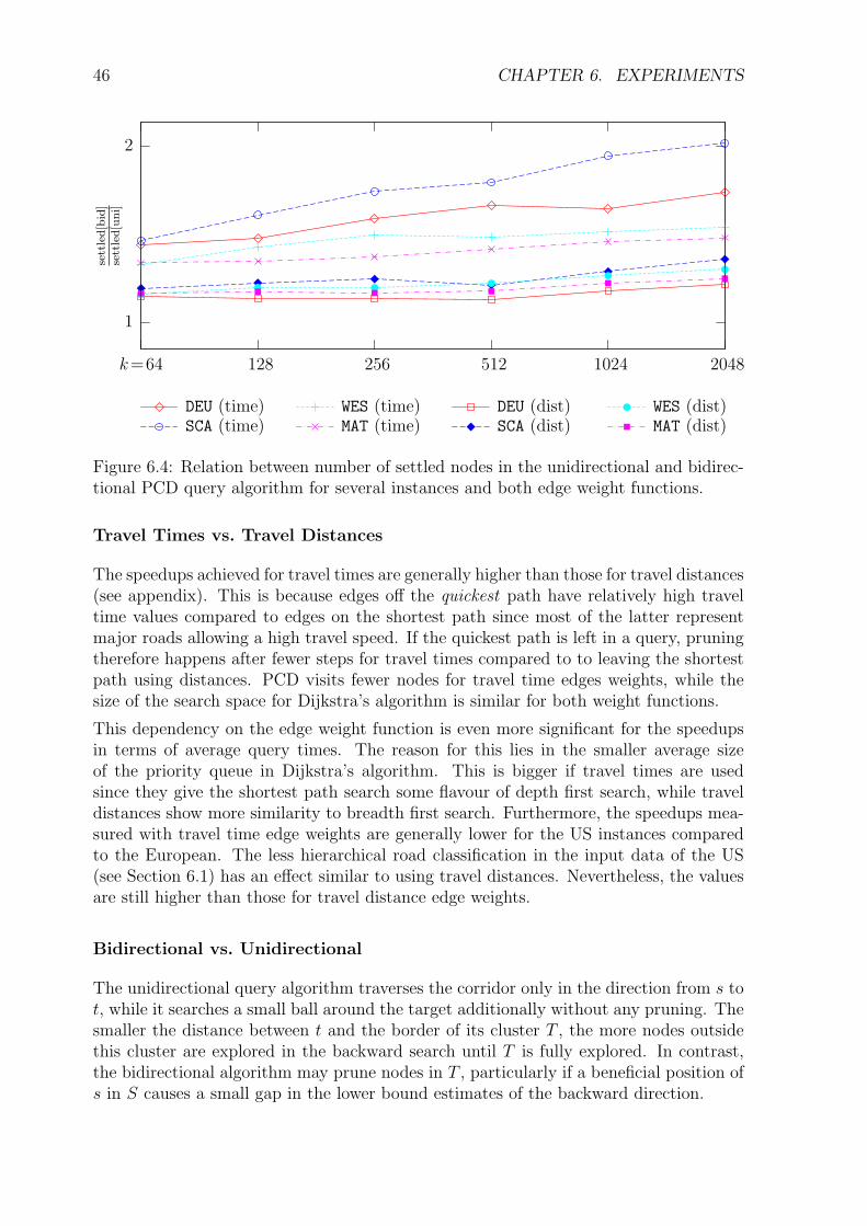
46 CHAPTER 6. EXPERIMENTS
1
2
20481024512256128k=64
sett
led[b
id]
sett
led[u
ni]
DEU (time)SCA (time)
WES (time)MAT (time)
DEU (dist)SCA (dist)
WES (dist)MAT (dist)
Figure 6.4: Relation between number of settled nodes in the unidirectional and bidirec-tional PCD query algorithm for several instances and both edge weight functions.
Travel Times vs. Travel Distances
The speedups achieved for travel times are generally higher than those for travel distances(see appendix). This is because edges off the quickest path have relatively high traveltime values compared to edges on the shortest path since most of the latter representmajor roads allowing a high travel speed. If the quickest path is left in a query, pruningtherefore happens after fewer steps for travel times compared to to leaving the shortestpath using distances. PCD visits fewer nodes for travel time edges weights, while thesize of the search space for Dijkstra’s algorithm is similar for both weight functions.
This dependency on the edge weight function is even more significant for the speedupsin terms of average query times. The reason for this lies in the smaller average sizeof the priority queue in Dijkstra’s algorithm. This is bigger if travel times are usedsince they give the shortest path search some flavour of depth first search, while traveldistances show more similarity to breadth first search. Furthermore, the speedups mea-sured with travel time edge weights are generally lower for the US instances comparedto the European. The less hierarchical road classification in the input data of the US(see Section 6.1) has an effect similar to using travel distances. Nevertheless, the valuesare still higher than those for travel distance edge weights.
Bidirectional vs. Unidirectional
The unidirectional query algorithm traverses the corridor only in the direction from s tot, while it searches a small ball around the target additionally without any pruning. Thesmaller the distance between t and the border of its cluster T , the more nodes outsidethis cluster are explored in the backward search until T is fully explored. In contrast,the bidirectional algorithm may prune nodes in T , particularly if a beneficial position ofs in S causes a small gap in the lower bound estimates of the backward direction.

6.3. EXPERIMENTAL RESULTS 47
(a) The green area in the interior is ex-plored by both, the surrounding red areaonly by the unidirectional, and the blackstrip at the right only by the bidirectionalversion.
(b) Position of the source node (left) andthe target node (right) in their respectiveclusters.
Figure 6.5: Search spaces of the unidirectional and the bidirectional algorithm for asample source-target pair.
Figure 6.4 illustrates the relation between the uni- and bidirectional query algorithm interms of average number of settled nodes. For travel distances, this relation is slightlygreater than one, which could be expected from the consideration above, while it goes upto two for travel times. Since major roads may lead the search to nodes far outside thetarget cluster T after few settling steps, the backward search might have to settle evenmore nodes outside T until it is fully explored for travel times. This is less significantfor the US instances due to the less hierarchical road classification. Furthermore, therelation rises with increasing k: the more clusters there are, the earlier and more oftenthe upper bound is updated, which takes stronger effect in the bidirectional query.
To sum up, the unidirectional algorithm is affected stronger by an adverse position of tin T , but cannot profit from the position of s in S unlike the bidirectional version. Theexample shown in Figure 6.5 further illustrates this issue: the source node’s positionclose to its cluster’s border causes the backward search to explore a narrow corridor,while the unidirectional algorithm traverses a wider corridor from left to right due tothe adverse position of the target. Moreover, there is a large ball around the target forthe unidirectional algorithm due to the target’s position close to the border. Analogouslyto Table 6.3, the values measured for the unidirectional PCD query algorithm can befound in Table 2 of the appendix.
6.3.2 Partitioning Methods
All results presented so far use (k log k)-clustering with the MinSize deletion heuristic forpartitioning the input graph. In the following this is compared with results for variantsof k′-oversampling and the other partitioning methods from Chapter 5. They all turnout to perform worse. All speedup values in this section are measured on the graph DEU
using travel time edge weights, while oversampling is performed with k′ = k log k unlessotherwise mentioned.

48 CHAPTER 6. EXPERIMENTS
0.35
0.42
0.5
0.59
0.71
0.84
20481024512256128k=64
spd
√k
MinSizeMinSizeRad
MinRadMETIS
Grid
Figure 6.6: Performance of PCD depending on the partitioning method.
Oversampling vs. Grid and METIS
Figure 6.6 compares the average speedups of several heuristics for (k log k)-oversamplingas well as grid clustering and METIS. Both METIS and the simple grid clustering approachperform better than the MinRad heuristic, but yield average speedups still smaller thanthose for the MinSizeRad heuristic. All these methods are well outperformed by theMinSize deletion heuristic.
Low cluster diameters improve the speedups since they reduce the gap in the lower boundestimates, and oversampling with the MinSize deletion heuristic indeed shows the lowestaverage cluster radius as can be seen in Figure 6.7. On the other hand, the plot showsthat the average radius does not fully reflect the quality of a partitioning. Oversamplingmay generally yield fairly low average diameters since the nodes of a deleted clustertend to be distributed to clusters with smaller radii. However, the average radius forthe MinRad heuristic suggests much better speedups, particularly compared to gridclustering, which also holds for METIS.
It seems that an ideal partitioning should have clusters of the same size and very lowin diameter. Nevertheless, a higher diameter is acceptable for a cluster with a smallnumber of nodes since, in such a case, only few nodes are affected by the worse lowerbound estimate, whereas a low diameter allows a bigger cluster size.
This is the idea that the MinSize heuristic implements: just after oversampling, i.e.before deletion has started, all clusters have a similar size, while their radii differ a lotwith lower values in urban areas. Since MinSize picks clusters regardless of their radius,deletion happens in all areas of the graph, and the way of redistributing causes high-diameter clusters to grow less. This can be verified in Figures 6.8 and 6.9, which showthat MinSize allows some deviation of the cluster sizes and a medium deviation of theradii. The crucial point is that clusters with a radius greater than the average consistof a number of nodes less than the average size, and vice versa.

6.3. EXPERIMENTAL RESULTS 49
16384
32768
65536
20481024512256128k=64
r avg
MinSizeMinSizeRad
MinRadMETIS
Grid
Figure 6.7: Average cluster radius ravg depending on the partitioning method.
0.25
0.5
1
20481024512256128k=64
σr
r avg
MinSizeMinSizeRad
MinRadMETIS
Grid
Figure 6.8: Deviation σr of the cluster radii in relation to the average cluster radius ravg
depending on the partitioning method.
0
0.5
1
1.5
2
20481024512256128k=64
σs
s avg
MinSizeMinSizeRad
MinRadMETIS
Grid
Figure 6.9: Deviation σs of the cluster sizes in relation to the average cluster size savg = nk
depending on the partitioning method.

50 CHAPTER 6. EXPERIMENTS
0.42
0.5
0.59
0.71
0.84
20481024512256128k=64
spd
√k
k′ = kk′ = k + 1
16∆
k′ = k + 14∆
k′ = k + 1∆ (= k log k)k′ = k + 4∆
Figure 6.10: Results for k′-oversampling with the MinSize deletion heuristic dependingon the value of k′.
In contrast, the MinRad heuristic keeps selecting clusters in urban areas and thus grow-ing urban clusters in size and radius, which results in clusters of similar radii but highlydiffering sizes (see Figures 6.8 and 6.9). The opposite holds for METIS: it yields a zero-deviation of the sizes, which must be paid for with some clusters of very high radius.
Choice of k′
The performance of k′-oversampling depends on the value of k′, which is illustrated inFigure 6.10. In this figure the value ∆ = k log k − k denotes the gap between k log kand k. Starting from k′ = k, which means just choosing k centers randomly, even asmall value of ∆ > 0 causes considerably higher speedups. Further increasing k′ alsoincreases the measured speedups, until values higher than k log k show no significantimprovement.
6.3.3 Border Nodes
Apart from the precomputed cluster distances, the cluster ids add to the space consump-tion for precomputed data, and must be stored for the B border nodes. As illustratedin Figure 6.11, this number B depends on the partitioning method, of which METISyields the fewest border nodes since one of its objectives is reducing the edge cut (seeSection 5.3). However, independent from the method, the amount of border nodes isnegligible compared to k2 for larger values of k since B = O(
√k). For lower k, the
value of B + k2 is very small anyway (also see Table 6.4), so the number of bordernodes B and therefore the partitioning method does not affect the space requirementsignificantly. This holds for oversampling in particular, further supporting its use as thereference method for graph partitioning in Section 6.3.1.

6.3. EXPERIMENTAL RESULTS 51
0.0977 %
0.391 %
1.56 %
6.25 %
25 %
100 %
20481024512256128k=64
B n
MinSizeMinSizeRad
MinRadGrid
METISk2
n
Figure 6.11: Relative number of border nodes depending on the method of partitioning.The numbers refer to DEU with travel time edge weights.
2
4
8
16
20481024512256128k=64pre
pro
cess
ing
tim
e[s
]/
k
DEU SCA WES MAT
Figure 6.12: Time required for precomputing the cluster distances (scaled by the numberof clusters k) using travel time edge weights.

52 CHAPTER 6. EXPERIMENTS
30 s
60 s
120 s
240 s
480 s
20481024512256128k=64
par
titi
onin
gti
me
MinSizeMinSizeRad
MinRadGrid
METIS
Figure 6.13: Partitioning time for several methods and varying k, measured for DEU
using travel time edge weights.
6.3.4 Preprocessing Time
Figure 6.12 shows the time needed for precomputing the cluster distances scales with kas expected from Chapter 3. Though DEU and WES are of similar size (see Tables 6.1 and6.2), their preprocessing times differ by a factor of about two, which holds for SCA andMAT analogously. Similar to the different speedups in terms of query time as explainedin Section 6.3.1, the less hierarchical road-classification of the US instances causes asmaller size of the priority queue and thus a faster preprocessing.
The partitioning times for several methods are presented in Figure 6.13: the oversam-pling heuristics need less than one minute for the fairly big graph instance DEU, againsupporting the role as the basis clustering technique throughout this chapter. ThoughMinSizeRad shows a somewhat unspecific behaviour, MinSize works slightly faster thanMinRad as expected from Section 5.1.2. Compared to oversampling, which estimatescluster radii while partitioning, the times for grid clustering and METIS are relatively highsince they compute the radii in an additional step as described in Section 5.4. Still, thepartitioning time is negligible compared to the time needed for computing the clusterdistances for all tested partitioning methods.

Chapter 7
Concluding Remarks
This last chapter concludes with summarising the main benefits of the algorithm andsuggesting potential improvements and applications. Furthermore, an outlook is givenon the prospects of future developments in combination with PCD.
7.1 Conclusion
The PCD algorithm is a new partitioning-based preprocessing heuristic to effectivelyreduce the search space of Dijkstra’s algorithm. Experiments on real-world road networkshave shown that the bidirectional variant using a k-center clustering performs best, andthe highest measured speedup is 114.9 in terms of query time. In addition, the speedupin terms of number of settled nodes is independent of the graph size.
PCD presents an interpolation between all pairs shortest paths and ordinary shortestpath search. The method’s favourable relation between speedup and space requirementallows significant speedups even for a sublinear amount of additional space. By itstuning parameter k, which directly determines the space requirement and preprocessingtime, the method offers a possibility to trade off between the contrary objectives ofpreprocessing costs and query speedups.
Since the k shortest path searches performed in the preprocessing are independent ofeach other, parallelising the preprocessing can be done straight-forwardly. This canparticularly be used for updates in dynamic settings, which might represent congestionsor roadworks in the example of street networks.
The algorithm is highly flexible as it works with arbitrary partitioning methods anddoes not afford a graph layout. Still, partitionings might be obtained by techniquesfrom computational geometry if a layout is given, and even the simple grid clusteringhas shown to perform reasonably well.
Finally, the precomputed cluster distances might not supply a potential function forA∗, but the search is directed towards the target by the PCD query algorithm too.Therefore, and for the algorithm’s simplicity, PCD is an alternative method to provideother acceleration techniques with goal-direction.
53

54 CHAPTER 7. CONCLUDING REMARKS
7.2 Future Work
There is still room for improvement regarding the PCD algorithm itself, possible parti-tioning methods, and particularly combinations with other speedup algorithms.
Query Algorithm
Presumably, a major improvement of the algorithm itself could be achieved by betterdistance bounds. The upper bounds are already very tight but can still be improvedby introducing dummy nodes that split edges crossing a border. This reduces someof the precomputed cluster distances since (parts of) longer edges crossing borders arethen not contained in the precomputed paths, which has an effect particularly if linesof degree-two nodes in the input graph are contracted. Perhaps, a similar effect mightbe achieved by defining partitionings in a way that border nodes are assigned to allsurrounding clusters(and thus edges do not cross borders).
For the bidirectional variant, the gaps in the lower bound estimates relating to the sourceand target clusters (see Section 1.3) could probably be reduced by using shortest pathinformation gained from the opposite search direction. Instead of using the shortestdistance to the target cluster in a forward step, the shortest distances to all clusterswith a node in the backward priority queue could be used if their number is small.Particularly, if all the nodes of one search frontier are in the same cluster, the respectivedirection might be stopped, and the opposite search directed to this cluster.
Partitioning Algorithms
There are several graph partitioning methods which would be interesting to combinewith PCD. Clustering techniques from computational geometry such as quadtrees orkd-trees (see e.g. [dBvKOS00]) might improve on the simple grid clustering. Besidessuitably implementing the notion of k-center clustering for directed graphs, establishingan objective function is desirable for partitionings applied to PCD in general, whichmight also be the key to successfully develop the local search for k-center clustering(see Section 5.1.3). In this connection, comparing existing k-center approximations tok′-oversampling might be helpful in finding the main parameters of a possible objectivefunction.
Combinations with Other Speedup Heuristics
The most promising prospect regarding the future work connected with PCD probably isproviding other search heuristics with goal-direction. While highway hierarchies [SS05,Sch05] do not naturally combine with A∗ search, their combination with PCD is straight-forward, so a further speedup of this very fast method seems possible with only slightlyincreasing the moderate space requirement.
The multi-level approach [SWZ02, KMS05] can also be combined with PCD. Both meth-ods perform some graph partitioning, and it would be interesting to find a partitioningmethod which is favourable to both approaches as well as their combination.

7.2. FUTURE WORK 55
Furthermore, landmark-based A∗ [GH05, GH04] and PCD yield similar speedup val-ues, and a combination of landmark-A∗ and reach-based pruning [GKW06, GKW05]is one of the currently most successful acceleration heuristics. Combining reach-basedpruning with PCD might possibly yield similar speedups at a significantly lower spaceconsumption. Besides, a bidirectional version of this combination will allow implicitbounding [GH05, GH04] unlike the combination with landmark-A∗.
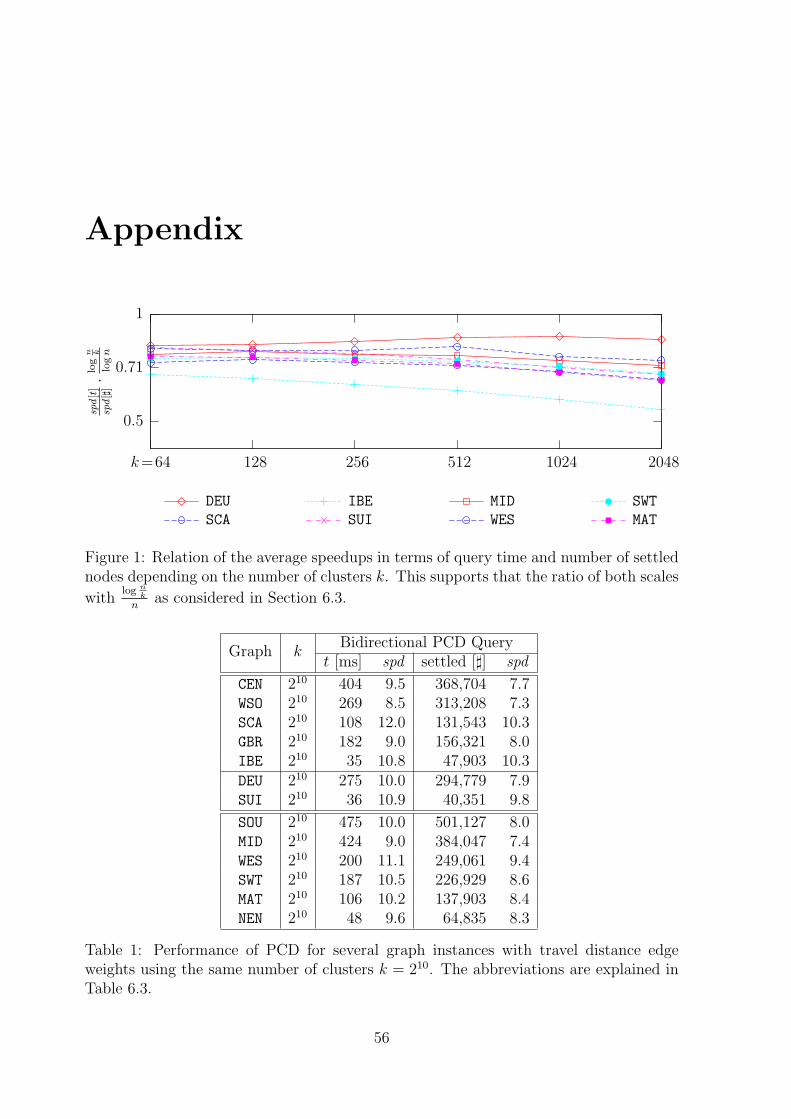
Appendix
0.5
0.71
1
20481024512256128k=64
spd[t]
spd[]
]·lo
gn k
log
n
DEU
SCA
IBE
SUI
MID
WES
SWT
MAT
Figure 1: Relation of the average speedups in terms of query time and number of settlednodes depending on the number of clusters k. This supports that the ratio of both scales
withlog n
k
nas considered in Section 6.3.
Bidirectional PCD QueryGraph k
t [ms] spd settled []] spd
CEN 210 404 9.5 368,704 7.7WSO 210 269 8.5 313,208 7.3SCA 210 108 12.0 131,543 10.3GBR 210 182 9.0 156,321 8.0IBE 210 35 10.8 47,903 10.3DEU 210 275 10.0 294,779 7.9SUI 210 36 10.9 40,351 9.8
SOU 210 475 10.0 501,127 8.0MID 210 424 9.0 384,047 7.4WES 210 200 11.1 249,061 9.4SWT 210 187 10.5 226,929 8.6MAT 210 106 10.2 137,903 8.4NEN 210 48 9.6 64,835 8.3
Table 1: Performance of PCD for several graph instances with travel distance edgeweights using the same number of clusters k = 210. The abbreviations are explained inTable 6.3.
56

7.2. FUTURE WORK 57
0.25
0.35
0.5
409620481024512256k=128
spd[]
]√
k
DEU SCA IBE SUI WES SWT MAT
Figure 2: Performance of PCD for several instances and varying numbers of clusters kusing travel distance edge weights. This shows that the speedups show the expectedsquareroot-growth for travel distances too.
Unidirectional PCD QueryGraph k
t [ms] spd settled []] spd
CEN 210 323 20.4 264,921 13.0WSO 210 298 13.7 281,775 9.7SCA 210 173 21.3 136,365 14.2GBR 210 114 25.0 110,002 16.4IBE 210 43 16.5 51,716 13.7DEU 210 256 21.2 199,663 13.2SUI 210 20 20.8 25,070 19.1
SOU 210 404 17.8 393,012 11.6MID 210 287 15.4 326,112 10.3WES 210 238 15.2 227,768 11.3SOU 210 183 17.5 172,433 12.4MAT 210 101 17.1 114,702 12.0NEN 210 39 15.1 49,259 11.6
Table 2: Performance of unidirectional PCD for several graph instances with travel timeedge weights using the same number of clusters k = 210 (corresponding to Table 6.3 forthe bidirectional version).
Bibliography
[AMOT90] Ravindra K. Ahuja, Kurt Mehlhorn, James Orlin, and Robert E. Tarjan.Faster algorithms for the shortest path problem. Journal of the ACM,37(2):213–223, 1990.
[BSWW04] Ulrik Brandes, Frank Schulz, Dorothea Wagner, and Thomas Willhalm.Generating node coordinates for shortest-path computations in transporta-tion networks. ACM Journal of Experimental Algorithmics, 9:1–16, 2004.(announced at ALENEX-01).
[CGS99] Boris V. Cherkassky, Andrew V. Goldberg, and Craig Silverstein. Buckets,heaps, lists, and monotone priority queues. SIAM Journal on Computing,28(4):1326–1346, 1999. (announced at SODA-97).
[CLRS01] Thomas H. Cormen, Charles E. Leiserson, Ronald L. Rivest, and CliffordStein. Introduction to Algorithms. The MIT Press, 2nd edition, 2001.
[dBvKOS00] Mark de Berg, Marc van Kreveld, Mark Overmars, and OttfriedSchwarzkopf. Computational Geometry – Algorithms and Applications.Springer, 2nd edition, 2000.
[Dia69] Robert B. Dial. Algorithm 360: Shortest-path forest with topological or-dering. Communications of the ACM, 12(11):632–633, 1969.
[Dij59] E. W. Dijkstra. A note on two problems in connexion with graphs. Nu-merische Mathematik, 1:269–271, 1959.
[Fre87] Greg N. Frederickson. Fast algorithms for shortest paths in planar graphs,with applications. SIAM Journal on Computing, 16(6):1004–1022, 1987.
[FT87] Michael L. Fredman and Robert E. Tarjan. Fibonacci heaps and theiruses in improved network optimization algorithms. Journal of the ACM,34(3):596–615, 1987.
[FW94] Michael L. Fredman and Dan E. Willard. Trans-dichotomous algorithmsfor minimum spanning trees and shortest paths. Journal of Computer andSystem Sciences, 48(3):533–551, 1994.
[GH04] Andrew V. Goldberg and Chris Harrelson. Computing the shortest path:A∗ search meets graph theory. Technical Report MSR-TR-2004-24, Mi-crosoft Research, Redmond, WA, March 2004.
58
BIBLIOGRAPHY 59
[GH05] Andrew V. Goldberg and Chris Harrelson. Computing the shortest path:A∗ search meets graph theory. In Proceedings of the 16th Annual ACM-SIAM Symposium on Discrete Algorithms (SODA-05), pages 156–165.SIAM, 2005.
[GKW05] Andrew V. Goldberg, Haim Kaplan, and Renato F. Werneck. Reach forA∗: Efficient point-to-point shortest path algorithms. Technical ReportMSR-TR-2005-132, Microsoft Research, Redmond, WA, October 2005.
[GKW06] Andrew V. Goldberg, Haim Kaplan, and Renato F. Werneck. Reach forA∗: Efficient point-to-point shortest path algorithms. In Proceedings of the8th Workshop on Algorithm Engineering and Experiments (ALENEX-06).SIAM, 2006.
[Gol01] Andrew V. Goldberg. A simple shortest path algorithm with linear averagetime. In Proceedings of the 9th Annual European Symposium on Algorithms(ESA-01), volume 2832 of Lecture Notes in Computer Science, pages 230–241. Springer, 2001.
[Gut04] Ronald J. Gutman. Reach-based routing: A new approach to shortest pathalgorithms optimized for road networks. In Proceedings of the 6th Work-shop on Algorithm Engineering and Experiments (ALENEX-04), pages100–111. SIAM, 2004.
[GW05] Andrew V. Goldberg and Renato F. Werneck. Computing point-to-pointshortest paths from external memory. In Proceedings of the 7th Workshopon Algorithm Engineering and Experiments (ALENEX-05), pages 26–40.SIAM, 2005.
[Hag98] Torben Hagerup. Sorting and searching on the word RAM. In Proceedingsof the 15th Annual Symposium on Theoretical Aspects of Computer Science(STACS-98), pages 366–398, London, UK, 1998. Springer.
[HKRS97] Monika R. Henzinger, Philip Klein, Satish Rao, and Sairam Subramanian.Faster shortest-path algorithms for planar graphs. Journal of Computerand System Sciences, 55(1):3–23, 1997. (announced at STOC-94).
[HNR68] P. E. Hart, N. J. Nilsson, and B. Raphael. A formal basis for the heuris-tic determination of minimum-cost paths. IEEE Transactions of SystemsScience and Cybernetics, SSC-4(2):100–107, July 1968.
[HNR72] P. E. Hart, N. J. Nilsson, and B. Raphael. Correction to “A formal basisfor the heuristic determination of minimum cost paths”. SIGART Bulletin,37:28–29, 1972.
[HSW04] Martin Holzer, Frank Schulz, and Thomas Willhalm. Combining speed-up techniques for shortest-path computations. In Proceedings of the 3rdInternational Workshop on Experimental and Efficient Algorithms (WEA-04), volume 3059 of Lecture Notes in Computer Science, pages 269–284.Springer, 2004.
60 BIBLIOGRAPHY
[Joh77] Donald B. Johnson. Efficient algorithms for shortest paths in sparse net-works. Journal of the ACM, 24(1):1–13, 1977.
[KH79] Oded Kariv and S. Louis Hakimi. An algorithmic approach to networklocation problems. I: The p-centers. Journal on Applied Mathematics,37(3):513–538, 1979.
[KK97] Hermann Kaindl and Gerhard Kainz. Bidirectional heuristic search recon-sidered. Journal of Artificial Intelligence Research, 7:283–317, 1997.
[KK98] George Karypis and Vipin Kumar. Multilevel k-way partitioning schemefor irregular graphs. Journal of Parallel and Distributed Computing,48(1):96–129, 1998.
[KMS05] Ekkehard Kohler, Rolf H. Mohring, and Heiko Schilling. Acceleration ofshortest path and constrained shortest path computation. In Proceedings ofthe 4th International Workshop on Experimental and Efficient Algorithms(WEA-05), volume 3503 of Lecture Notes in Computer Science, pages 126–138. Springer, 2005.
[Lau04] Ulrich Lauther. An extremely fast, exact algorithm for finding shortestpaths in static networks with geographical backgrounds. In Geoinformationund Mobilitat - Von der Forschung zur praktischen Anwendung, volume 22of IfGIprints, 2004.
[Met95] Metis: A software package for partitioning unstructured graphs, parti-tioning meshes, and computing fill-reducing orderings of sparse matrices.http://glaros.dtc.umn.edu/gkhome/views/metis, 1995.
[Mey03] Ulrich Meyer. Average-case complexity of single-source shortest-path algo-rithms: lower and upper bounds. Journal of Algorithms, 48:91–134, 2003.(announced at SODA-01).
[MN99] Kurt Mehlhorn and Stefan Naher. LEDA - A Platform for Combinatorialand Geometric Computing. Cambridge University Press, Cambridge, UK,1999.
[MSM06] Jens Maue, Peter Sanders, and Domagoj Matijevic. Goal directed shortestpath queries using precomputed cluster distances. In Proceedings of the 5thInternational Workshop on Experimental Algorithms (WEA-06), volume4007 of Lecture Notes in Computer Science, pages 316–327. Springer, 2006.
[MSS+05] Rolf H. Mohring, Heiko Schilling, Birk Schutz, Dorothea Wagner, andThomas Willhalm. Partitioning graphs to speed up dijkstra’s algorithm.In Proceedings of the 4th International Workshop on Experimental andEfficient Algorithms (WEA-05), volume 3503 of Lecture Notes in ComputerScience, pages 189–202. Springer, 2005.
[Poh71] Ira Pohl. Bi-directional search. In Machine Intelligence, volume 6, pages127–140. Edinburgh University Press, 1971.

BIBLIOGRAPHY 61
[Ram97] Rajeev Raman. Recent results on the single-source shortest paths problem.ACM SIGACT News, 28(2):81–87, 1997.
[Sch05] Dominik Schultes. Fast and exact shortest path queries using highwayhierarchies. Master-Arbeit, Universitat des Saarlandes, Saarbrucken, July2005.
[SS05] Peter Sanders and Dominik Schultes. Highway hierarchies hasten exactshortest path queries. In Proceedings of the 13th Annual European Sympo-sium on Algorithms (ESA-05), volume 3669 of Lecture Notes in ComputerScience, pages 568–579. Springer, 2005.
[SWW00] Frank Schulz, Dorothea Wagner, and Karsten Weihe. Dijkstra’s algorithmon-line: An empirical case study from public railroad transport. ACMJournal of Experimental Algorithms, 5, 2000.
[SWZ02] Frank Schulz, Dorothea Wagner, and Christos D. Zaroliagis. Using multi-level graphs for timetable information. In Proceedings of the 4th Interna-tional Workshop on Algorithm Engineering and Experiments (ALENEX-02), volume 2409 of Lecture Notes in Computer Science, pages 43–59.Springer, 2002.
[Tho99] Mikkel Thorup. Undirected single-source shortest paths with positive in-teger weights in linear time. Journal of the ACM, 46(3):362–394, 1999.(announced at FOCS-97).
[Tho00] Mikkel Thorup. On RAM priority queues. SIAM Journal on Computing,30(1):86–109, 2000. (announced at SODA-96).
[Tho04] Mikkel Thorup. Integer priority queues with decrease key in constant timeand the single source shortest paths problem. Journal of Computer andSystem Sciences, 69(3):330–353, 2004. (announced at STOC-03).
[U.S02] U.S. Census Bureau, Washington, DC. UA Census 2000 TIGER/LineFiles. http://www.census.gov/geo/www/tiger/tigerua/ua_tgr2k.
html, 2002.
[vEB77] Peter van Emde Boas. Preserving order in a forest in less than logarithmictime and linear space. Information Processing Letters, 6(3):80–82, 1977.
[vEBKZ77] Peter van Emde Boas, R. Kaas, and E. Zijlstra. Design and implementationof an efficient priority queue. Mathematical Systems Theory, 10:99–127,1977.
[WW03] Dorothea Wagner and Thomas Willhalm. Geometric speed-up techniquesfor finding shortest paths in large sparse graphs. In Proceedings of the11th Annual European Symposium on Algorithms (ESA-03), volume 2832of Lecture Notes in Computer Science, pages 776–787. Springer, 2003.

62 BIBLIOGRAPHY
[WW05] Dorothea Wagner and Thomas Willhalm. Drawing graphs to speed upshortest-path computations. In Proceedings of the 7th Workshop on Algo-rithm Engineering and Experiments (ALENEX-05), 2005.
[WWZ04] Dorothea Wagner, Thomas Willhalm, and Christos Zaroliagis. Dynamicshortest path containers. In Proceedings of the 3rd Workshop on Algo-rithmic Methods and Models for Optimization of Railways (ATMOS-03),volume 92 of Electronic Notes in Theoretical Computer Science, pages 65–84. Elsevier, 2004.
[WWZ05] Dorothea Wagner, Thomas Willhalm, and Christos Zaroliagis. Geometriccontainers for efficient shortest-path computation. Journal of ExperimentalAlgorithmics, 10:1–30, 2005.