A geometric approach to dynamical model order reduction · A GEOMETRIC APPROACH TO DYNAMICAL...

A GEOMETRIC APPROACH TODYNAMICAL MODEL–ORDER REDUCTION

FLORIAN FEPPON AND PIERRE F.J. LERMUSIAUX∗

Abstract. Any model order reduced dynamical system that evolves a modal decomposition toapproximate the discretized solution of a stochastic PDE can be related to a vector field tangentto the manifold of fixed rank matrices. The Dynamically Orthogonal (DO) approximation is thecanonical reduced order model for which the corresponding vector field is the orthogonal projectionof the original system dynamics onto the tangent spaces of this manifold. The embedded geometry ofthe fixed rank matrix manifold is thoroughly analyzed. The curvature of the manifold is characterizedand related to the smallest singular value through the study of the Weingarten map. Differentiabilityresults for the orthogonal projection onto embedded manifolds are reviewed and used to derive anexplicit dynamical system for tracking the truncated Singular Value Decomposition (SVD) of atime-dependent matrix. It is demonstrated that the error made by the DO approximation remainscontrolled under the minimal condition that the original solution stays close to the low rank manifold,which translates into an explicit dependence of this error on the gap between singular values. TheDO approximation is also justified as the dynamical system that applies instantaneously the SVDtruncation to optimally constrain the rank of the reduced solution. Riemannian matrix optimizationis investigated in this extrinsic framework to provide algorithms that adaptively update the best lowrank approximation of a smoothly varying matrix. The related gradient flow provides a dynamicalsystem that converges to the truncated SVD of an input matrix for almost every initial data.

Key words. Model order reduction, fixed rank matrix manifold, low rank approximation,Singular Value Decomposition, orthogonal projection, curvature, Weingarten map, Dynamically Or-thogonal approximation, Riemannian matrix optimization.

AMS subject classifications. 65C20, 53B21, 65F30, 15A23, 53A07, 35R60, 65M15

1. Introduction. Finding efficient model order reduction methods is an issuecommonly encountered in a wide variety of domains involving intensive computa-tions and expensive high-fidelity simulations [66, 61, 38, 13]. Such domains includeuncertainty quantification [25, 46, 69, 72], dynamical systems analysis [30, 9, 80], elec-trical engineering [24, 8], mechanical engineering [54], ocean and weather predictions[41, 49, 12, 62], chemistry [55], and biology [40], to name a few. The computationalcosts and challenges arise from the complexity of the mathematical models as wellas from the needs of representing variations of parameter values and the dominantuncertainties involved. For example, to quantify uncertainties of dynamical systemfields, one often needs to solve stochastic partial differential equations (PDEs),

(1) ∂tu = L (t,u;ω) ,

where t is time, u the uncertain dynamical fields, L a differential operator, andω a random event. For deterministic but parametric dynamical systems, ω mayrepresent a large set of possible parameter values that need to be accounted for bythe model-order reduction. Generally, after both spatial and stochastic/parametricevent discretization of the PDE (1), or more directly if the focus is on solving acomplex system of ordinary differential equations (ODEs), one is interested in thenumerical solution of a large system of ODEs of the form

(2) R = L(t,R),

where L is an operator acting on the space of l-by-m matrices R. In the case ofa direct Monte-Carlo approach for the resolution of the stochastic PDE (1), L is

∗MSEAS, Massachusetts Institute of Technology ([email protected], [email protected]).

1

arX

iv:1

705.

0852

1v1

[m

ath.

DS]

23

May

201

7

mailto:[email protected]

mailto:[email protected]

2 F. FEPPON AND P.F.J. LERMUSIAUX

thought as being the discretization of the differential operator L by using l spatialnodes and m Monte-Carlo realizations or parameter values being considered. Accuratequantification of the statistical/parametric properties of the original solution u oftenrequire to solve such system (2) with both a high spatial resolution, l, and highnumber of realizations, m. Hence, solving (2) directly with a Monte-Carlo approachbecomes quickly intractable for realistic, real-time applications such as ocean andweather predictions [57, 44] or real-time control [39, 47].

A method to address this challenge is to assume the existence of an approximationuDO of the solution u onto a finite number of r spatial modes, ui(t, x), and stochasticcoefficients, ζi(t, ω) (here assumed to be both time-dependent [44, 64]),

(3) u(t,x;ω) ' uDO =

r∑i=1

ζi(t, ω)ui(t,x),

and look for a dynamical system that would most accurately govern the evolution ofthese dominant modes and coefficients. The optimal approximation (in the sense thatthe L2 error E[||u−uDO||2]1/2 is minimized) is achieved by the Karuhnen-Loeve (KL)decomposition [48, 30], whose first r modes yields an optimal orthonormal basis (ui).Many methods, such as polynomial chaos expansions [82], Fourier decomposition [79],or Proper Orthogonal Decomposition [30] rely on the choice of a predefined, time-independent orthonormal basis either for the modes, (ui), or the coefficients, (ζi),and obtain equations for the respective unknown coefficients or modes by Galerkinprojection [58]. However, the use of modes and coefficients that are simultaneouslydynamic has been shown to be efficient [44, 45]. Dynamically Orthogonal (DO) fieldequations [64, 65] were thus derived to evolve adaptively this decomposition for ageneral differential operator L and allowed to obtain efficient simulations of stochasticNavier-Stokes equations [73].

At the discrete level, the decomposition (3) is written R ' R = UZT whereR is a rank r approximation of the full rank matrix R, decomposed as the productof a l-by-r matrix U containing the discretization of the basis functions, (ui), andof a m-by-r matrix Z containing the realizations of the stochastic coefficients, (ζi).It is well known that such approximation is optimal (in the Frobenius norm) whenR = UZT is obtained by truncating the Singular Value Decomposition (SVD), i.e. byselecting U to be the singular vectors associated with the r largest singular valuesof R and setting Z = RTU [32, 31]. In 2007, Koch and Lubich [37] proposed amethod inspired from the Dirac Frenkel variational principle in quantum physics, toevolve dynamically a rank r matrix R = UZT that approximates the full dynamicalsystem (2). The main principle of the method lies in the intuition that one can updateoptimally the low-rank approximation R by projecting L(t, R) onto the tangent spaceof the manifold constituted by low rank matrices. Recently, Musharbash [52] noticedthe parallel with the DO method, and applied the results obtained in [37] to analyzethe error committed by the DO approximation for a stochastic heat equation. Infact, in the same way the KL expansion is the continuous analogous of the SVD, thediscretization of the DO decomposition [64] is strictly equivalent to the dynamicallow rank approximation of Koch and Lubich [37] when the discretization reduces tosimulate the matrix dynamical system (2) of m realizations spatially resolved with lnodes.

Simultaneously, new approaches have emerged since the 1990s in optimizationonto matrix sets [18, 3]. The application of Riemannian geometry to manifolds of ma-trices has allowed the development of new optimization algorithms, that are evolving

A GEOMETRIC APPROACH TO DYNAMICAL MODEL–ORDER REDUCTION 3

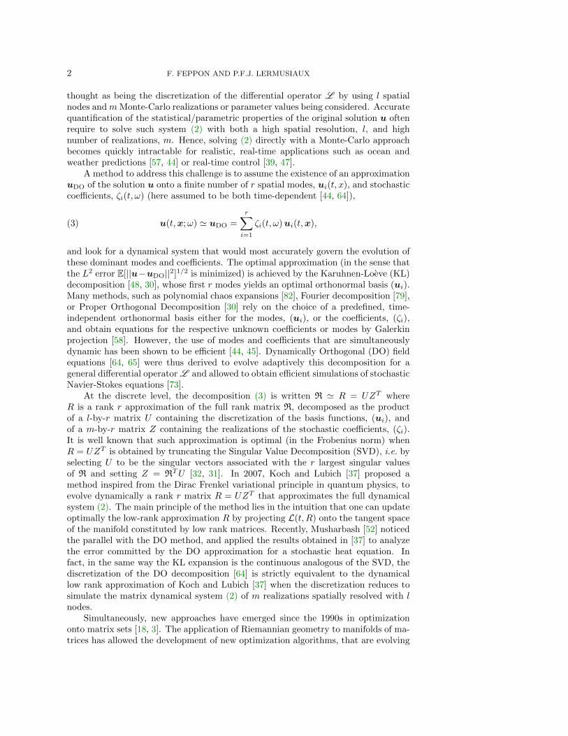
(a) R(ρ, πρ, φ) (b) R(ρ, φ, ρ− φ)

Fig. 1: Two subsurfaces of the rank-1 manifold M of 2-by-2 matrices.

orthogonality constraints geometrically rather than using more classical techniques,such as Lagrange multiplier methods [18]. Matrix dynamical systems that continu-ously perform matrices operations, such as inversion, eigen- or SVD-decompositions,steepest descents, and gradient optimization have thus been proposed [10, 14, 70].These continuous–time systems were extended and applied to adaptive uncertaintypredictions, learning of dominant subspace, and data assimilation [42, 43].

The purpose of this article is to extend the analysis and the understanding of theDO method in the matrix framework as initiated by [37] and in the above works, byfurthering its relation to the Singular Value Decomposition and its geometric inter-pretation as a constrained dynamics on the manifold M of fixed rank matrices. Inthe vein of [18, 3, 50], this article utilizes the point of view of differential geometry.To provide a visual intuition, a 3D projection of two 2-dimensional subsurfaces of themanifold M of rank one 2-by-2 matrices is visible on Figure 1. This figure has beenobtained by using the parameterization

R(ρ, θ, φ) = ρ

(sin(θ) sin(φ) sin(θ) cos(φ)cos(θ) sin(φ) cos(θ) cos(φ)

), ρ > 0, θ ∈ [0, 2π], φ ∈ [0, 2π],

on M and projecting orthogonally two subsurfaces by plotting the first three elementsR11, R12 and R21. Since the multiplication of singular values by a non-zero constantdoes not affect the rank of a matrix, M ⊂ M2,2 is a cone, which is consistent withthe increasing of curvature visible on Figure 1a near the origin. More generally, Mis the union of r-dimensional affine subspaces of Ml,m supported by the manifold ofstrictly lower rank matrices. It will actually be proven in section 4 that the curvatureof M is inversely proportional to the lowest singular value, which diverges as matricesapproach a rank strictly less than r. Hence M can be understood either as a collectionof cones (Figure 1b) or as a multidimensional spiral (Figure 1a). Geometrically, adynamical system (2) can be seen as a time dependent vector field L that assignsthe velocity L(t,R) at time t at each point R of the ambient space Ml,m of l-by-mmatrices (Figure 2a). Similarly, any rank r model order reduction can be viewed as avector field L that must be everywhere tangent to the manifold M of rank r matrices.The corresponding dynamical system is

(4) R = L(t, R) ∈ T (R),

where T (R) denotes the tangent space of M at R.


(a) Dynamical systems as vector fields L in the ambient space Ml,m (inred), or L tangent to M (in blue). The DO approximation sets L to bethe projection of L tangent to M .

(b) Geometric concepts of interest: orthogonal projection X = ΠT (R)Xof an ambient vector X ∈ Ml,m onto the tangent space T (R) of M atR. Orthogonal projection ΠM (R) of the point R onto M . Normal spaceN (R). Geodesic curve expR(tX) starting from R in the direction X.

Fig. 2: Vector fields on the fixed rank manifold M . Schematic adapted from [78].


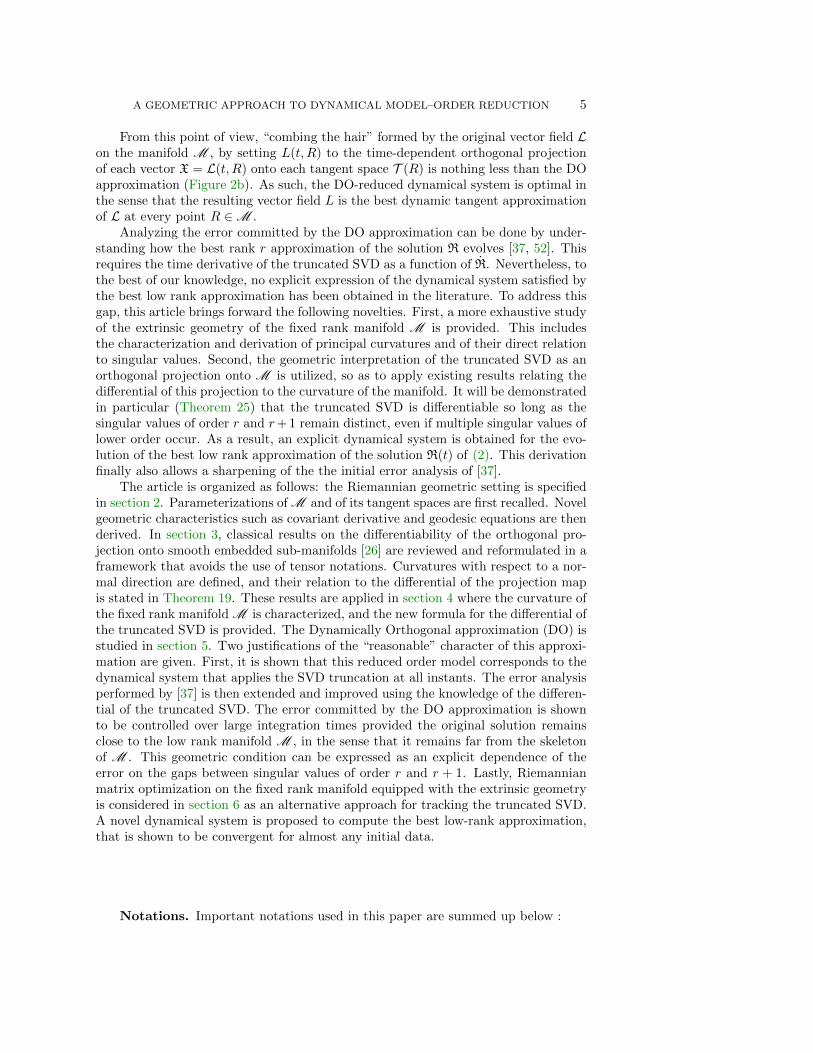
From this point of view, “combing the hair” formed by the original vector field Lon the manifold M , by setting L(t, R) to the time-dependent orthogonal projectionof each vector X = L(t, R) onto each tangent space T (R) is nothing less than the DOapproximation (Figure 2b). As such, the DO-reduced dynamical system is optimal inthe sense that the resulting vector field L is the best dynamic tangent approximationof L at every point R ∈M .

Analyzing the error committed by the DO approximation can be done by under-standing how the best rank r approximation of the solution R evolves [37, 52]. Thisrequires the time derivative of the truncated SVD as a function of R. Nevertheless, tothe best of our knowledge, no explicit expression of the dynamical system satisfied bythe best low rank approximation has been obtained in the literature. To address thisgap, this article brings forward the following novelties. First, a more exhaustive studyof the extrinsic geometry of the fixed rank manifold M is provided. This includesthe characterization and derivation of principal curvatures and of their direct relationto singular values. Second, the geometric interpretation of the truncated SVD as anorthogonal projection onto M is utilized, so as to apply existing results relating thedifferential of this projection to the curvature of the manifold. It will be demonstratedin particular (Theorem 25) that the truncated SVD is differentiable so long as thesingular values of order r and r+ 1 remain distinct, even if multiple singular values oflower order occur. As a result, an explicit dynamical system is obtained for the evo-lution of the best low rank approximation of the solution R(t) of (2). This derivationfinally also allows a sharpening of the the initial error analysis of [37].

The article is organized as follows: the Riemannian geometric setting is specifiedin section 2. Parameterizations of M and of its tangent spaces are first recalled. Novelgeometric characteristics such as covariant derivative and geodesic equations are thenderived. In section 3, classical results on the differentiability of the orthogonal pro-jection onto smooth embedded sub-manifolds [26] are reviewed and reformulated in aframework that avoids the use of tensor notations. Curvatures with respect to a nor-mal direction are defined, and their relation to the differential of the projection mapis stated in Theorem 19. These results are applied in section 4 where the curvature ofthe fixed rank manifold M is characterized, and the new formula for the differential ofthe truncated SVD is provided. The Dynamically Orthogonal approximation (DO) isstudied in section 5. Two justifications of the “reasonable” character of this approxi-mation are given. First, it is shown that this reduced order model corresponds to thedynamical system that applies the SVD truncation at all instants. The error analysisperformed by [37] is then extended and improved using the knowledge of the differen-tial of the truncated SVD. The error committed by the DO approximation is shownto be controlled over large integration times provided the original solution remainsclose to the low rank manifold M , in the sense that it remains far from the skeletonof M . This geometric condition can be expressed as an explicit dependence of theerror on the gaps between singular values of order r and r + 1. Lastly, Riemannianmatrix optimization on the fixed rank manifold equipped with the extrinsic geometryis considered in section 6 as an alternative approach for tracking the truncated SVD.A novel dynamical system is proposed to compute the best low-rank approximation,that is shown to be convergent for almost any initial data.

Notations. Important notations used in this paper are summed up below :


Ml,m Space of l-by-m real matricesM∗m,r Space of m-by-r matrices that have full rankrank(R) Rank of a matrix R ∈Ml,m

M = R ∈Ml,m|rank(R) = r Fixed rank matrix manifoldOr = P ∈Mr,r | PTP = I Group of r-by-r orthogonal matricesStl,r = U ∈Ml,r | UTU = I Stiefel ManifoldR = UZT Point R ∈M with U ∈ Stl,r and Z ∈M∗m,rT (R) Tangent space at R ∈MX ∈ T (R) Tangent vector X at R = UZT

H(U,Z) Horizontal space at R = UZT

(XU , XZ) ∈ H(U,Z) X = XUZT + UXT

Z ∈ T (R) withXU ∈Ml,r, XZ ∈Mm,r and UTXU = 0

ΠT (R) Orthogonal projection onto the plane T (R)Sk(M ) Skeleton of MΠM Orthogonal projection onto M (defined on Ml,m\Sk(M ))I Identity mappingAT Transpose of a square matrix A〈A,B〉 = Tr(ATB) Frobenius matrix scalar product||A|| = Tr(ATA)1/2 Frobenius normσ1(A) ≥ . . . ≥ σrank(A)(A) Non zeros singular values of A ∈Ml,m

R = dR/dt Time derivative of a trajectory R(t)DXf(R) Differential of a function f in direction XDΠT (R)(X) · Y Differential of the projection operator ΠT (R) applied to Y

The differential of a smooth function f at the point R ∈ Ml,m (respectivelyR ∈M ) in the direction X ∈Ml,m (respectively X ∈ T (R)) is denoted DXf(R):

(5) DXf(R) =d

dtf(R(t))

∣∣∣∣t=0

= lim∆t→0

f(R(t+ ∆t))− f(R(t))

∆t,

where R(t) is a curve of Ml,m (respectively M ) such that R(0) = R and R(0) = X.The differential of the orthogonal projection operator R 7→ ΠT (R) at R ∈M , in thedirection X ∈ T (R) and applied to Y ∈Ml,m is denoted DΠT (R)(X) · Y :

(6) DΠT (R)(X) · Y =

[d

dtΠT (R(t))

∣∣∣∣t=0

](Y ) =

[lim

∆t→0

ΠT (R(t+∆t)) −ΠT (R(t))

∆t

](Y ),

where R(t) is a curve drawn on M such that R(0) = R and R(0) = X.

2. Riemannian set up: parameterizations, tangent-space, geodesics.This section establishes the geometric framework of low-rank approximation, by re-viewing and unifying results sparsely available in [37, 64, 52], and by providing newexpressions for classical geometric characteristics, namely geodesics and covariantderivative. It is not assumed that the reader is accustomed to differential geometry:necessary definitions and properties are recalled. Several concepts of this section areillustrated on Figure 2b.

Definition 1. The manifold of l-by-m matrices of rank r is denoted by M :

M = R ∈Ml,m|rank(R) = r.

Remark 2. The fact that M is a manifold is a consequence of the constant ranktheorem ([71], Th.10, chap.2, vol. 1) whose assumptions (the map (U,Z) 7→ UZT

from Stl,r ×M∗m,r to M is a submersion with differential of constant rank) translatein the requirement that the candidate tangent spaces have constant dimension, asfound later in Proposition 4. Detailed proofs are available in [71] (exercise 34, chap.2, vol. 1) or [75] (Prop. 2.1).


The following lemma [60] fixes the parametrization of M by conveniently representingits elements R in terms of mode and coefficient matrices, U and Z, respectively.

Lemma 3. Any matrix R ∈M can be decomposed as R = UZT where U ∈ Stl,rand Z ∈ M∗m,r, i.e. UTU = I and rank(Z) = r, respectively. Furthermore, thisdecomposition is unique modulo a rotation matrix P ∈ Or, namely if U1, U2 ∈ Ml,r,Z1, Z2 ∈Mm,r, and UT1 U1 = UT2 U2 = I, then

(7) U1ZT1 = U2Z

T2 ⇔ ∃P ∈ Or, U1 = U2P and Z1 = Z2P.

In the following, the statement “let UZT ∈M ” always implicitly assumes U ∈Ml,r,Z ∈ Mm,r, U

TU = I, and rank(Z) = r. Other parameterizations of M are possibleand give equivalent results [50].

The tangent space T (UZT ) at a point R = UZT is the set of all possible vectorstangent to smooth curves R(t) = U(t)Z(t)T drawn on the manifold M . Therefore,such tangent vector at R(0) = UZT is of the form R = UZT + UZT , where U andZ are the time derivatives of the matrices U(t) and Z(t) at time t = 0. In thefollowing, the notations XU , XZ , and X = XUZ

T + UXTZ will be used to denote

the tangent directions U , Z, and R for the respective matrices U , Z and R. Theorthogonality condition that UTU = I must hold for all times implies that XU mustsatisfy UTU + UT U = XT

UU + UTXU = 0.Nevertheless, this is not sufficient to parameterize uniquely tangent vectors X

from the displacements XU and XZ for U and Z: two different couples (XU , XZ) 6=(X ′U , X

′Z) satisfying XT

UU + UTXU = X′TU U + UTX ′U = 0 may exist for a single

tangent vector X = XUZT + UXT

Z = X ′UZT + UX

′TZ . Indeed, rotations U ← UP

of the columns of the mode matrix U do not change the subspace span(ui) sup-porting the modal decomposition (3), and hence can be captured by updating thevalues of the coefficients (ζi) contained in the matrix Z with the same rotationZ ← ZP . This translates infinitesimally in the tangent space by the invarianceof tangent vectors X = XUZ

T + UXTZ under the transformations XU ← XU + UΩ

and XZ ← XZ + ZΩ for any skew-symmetric matrix Ω = −ΩT . This can easily beseen by inserting the transformations into the expression for X or by differentiatingthe relation UZT = (UP )(ZP )T with P = ΩP . A unique parameterization of thetangent space can be obtained by fixing this infinitesimal rotation Ω, for example byadding the condition that the reduced subspace spanned by the columns of U mustdynamically evolve orthogonally to itself, in other words by requiring UTXU = 0.This gauge condition has thus been called “Dynamically Orthogonal” condition by[64] and is at the origin of the name “Dynamically Orthogonal approximation” asfurther investigated in section 5.

Proposition 4. The tangent space of M at R = UZT ∈M is the set

(8) T (UZT ) = XUZT + UXT

Z | XU ∈Ml,r, XZ ∈Mm,r, UTXU +XT

UU = 0.

T (UZT ) is uniquely parameterized by the horizontal space

(9) H(U,Z) = (XU , XZ) ∈Ml,r ×Mm,r | UTXU = 0,

that is for any tangent vector X ∈ T (UZT ), there exists a unique (XU , XZ) ∈ H(U,Z)

such that X = XUZT+UXT

Z . As a consequence M is a smooth manifold of dimensiondim(H(U,Z)) = (l +m)r − r2.


Proof. (see also [37, 3]) One can always write a tangent vector X as

X = UZT + UZT

= U(ZT + UT UZT ) + ((I − UUT )U)ZT = XUZT + UXT

Z ,

for some U ∈ Stl,r and Z ∈Mm,r with XU = (I−UUT )UZT satisfying XTUU = 0 and

XTZ = ZT + UT UZT . This implies T (UZT ) = XUZ

T + UXTZ |(XU , XZ) ∈ H(U,Z).

Furthermore, if X = UXTZ +XUZ

T with UTXU = 0, then the relations XZ = XTUand XU = (I − UUT )XZ(ZTZ)−1 show that (XU , XZ) ∈ H(U,Z) is defined uniquelyfrom X.

Remark 5. The denomination “horizontal space” for the set H(U,Z) (9) refers tothe definition of a non-ambiguous representation of the tangent space T (UZT ) (8).This notion is developed rigorously in the theory of quotient manifolds e.g. [50, 18].

In the following, the notation X = (XU , XZ) is used equivalently to denote a tangentvector X = XUZ

T + UXTZ ∈ T (UZT ), where UTXU = 0 is implicitly assumed.

A metric is needed to define how distances are measured on the manifold, byprescribing a smoothly varying scalar product on each tangent space. In [50] andothers in matrix optimization e.g. [5, 75, 67], one uses the metric induced by theparametrization of the manifold M : the norm of a tangent vector (XU , XZ) ∈ H(U,Z)

is defined to be ||(XU , XZ)||2 = ||XU ||2Stl,r+ ||XZ ||2Mm,r

where || ||Stl,r is a canonical

norm on the Stiefel Manifold (see [18]) and || ||Mm,ris the Frobenius norm onMm,r.

In this work, one is rather interested in the metric inherited from the ambient full spaceMl,m, since it is the metric used to estimate the distance from a matrix R ∈ Ml,m

to its best r-rank approximation, namely the error committed by the truncated SVD.

Definition 6. At each point UZT ∈M , the metric g on M is the scalar productacting on the tangent space T (UZT ) that is inherited from the scalar product ofMl,m :

(10)g((XU , XZ), (YU , YZ)) = Tr((XUZ

T + UXTZ )T (YUZ

T + UY TZ ))

= Tr(ZTZXTUYU +XT

ZYZ).

A main object of this paper is the orthogonal projection ΠT (R) onto the tangent

space T (R) at a point R on M . This map projects displacements X = R ∈Ml,m of amatrix R of the ambient spaceMl,m to the tangent directions X = ΠT (R)X ∈ T (R).

Proposition 7. At every point UZT ∈ M , the orthogonal projection ΠT (UZT )

onto the tangent space T (UZT ) is the application

(11)ΠT (UZT ) : Ml,m → H(U,Z)

X 7→ ((I − UUT )XZ(ZTZ)−1,XTU).

Proof. (see also [37]) ΠT (R)X is obtained as the unique minimizer of the convex

functional J(XU , XZ) = 12 ||X−XUZ

T −UXTZ ||2 on the space H(U,Z). The minimizer

(XU , XZ) is characterized by the vanishing of the gradient of J :

∀∆ ∈Ml,r, ∆TU = 0⇒ ∂J

∂XU·∆ = −〈X−XUZ

T − UXTZ ,∆Z

T 〉 = 0,

∀∆ ∈Mm,r,∂J

∂XZ·∆ = −〈X−XUZ

T − UXTZ , U∆T 〉 = 0,

yielding respectively XU = (I − UUT )XZ(ZTZ)−1 and XZ = XTU .


The orthogonal complement of the tangent space T (R) is obtained from the identity(I −ΠT (UZT )) · X = (I − UUT )X(I − Z(ZTZ)−1ZT ):

Definition 8. The normal space N (R) of M at R = UZT is defined as theorthogonal complement to the tangent space T (R). For the fixed rank manifold M :

(12)N (R) = N ∈Ml,m|(I − UUT )N(I − Z(ZTZ)−1ZT ) = N

= N ∈Ml,m | UTN = 0 and NZ = 0.

In model order reduction, a matrix R = UZT ∈ M is usually a low rank-r approx-imation of a full rank matrix R ∈ Ml,m. The following proposition shows that thenormal space at R, N (R), can be understood as the set of all possible completions ofthe approximation (3):

Proposition 9. Let N be a given normal vector N ∈ N (R) at R = UZT ∈Mand denote k = rank(N). Then there exists an orthonormal basis of vectors (ui)1≤i≤lin Rl, an orthonormal basis (vi)1≤i≤m of Rm, and r + k non zero singular values(σi)1≤i≤r+k such that

(13) UZT =

r∑i=1

σiuivTi and N =

k∑i=1

σr+iur+ivTr+i.

Proof. Consider N = UNΘV TN the SVD decomposition of N [31]. Since UTN = 0,r columns of UN are spanned by U and associated with zero singular values of N ,therefore ui is obtained from the columns of U for 1 ≤ i ≤ r and from the left singularvectors of N associated with non zero singular values for r + 1 ≤ i ≤ r + k, k ≥ 0.The vectors vi and vr+j are obtained similarly. The singular values σi are obtainedby reunion of the respective r and k non-zeros singular values of Z and N .

In differential geometry, one distinguishes the geometric properties that are intrinsic,i.e. that depend only on the metric g defined on the manifold, from the ones thatare extrinsic, i.e. that depend on the ambient space in which the manifold M isdefined. The following proposition recalls the link between the extrinsic projectionΠT (R) and the intrinsic notion of derivation onto a manifold. For embedded manifolds,i.e. defined as subsets of an ambient space, the covariant derivative at R ∈ M isobtained by projecting the usual derivative onto the tangent space T (R), and theChristoffel symbol corresponds to the normal component that has been removed [18].

Proposition 10. Let X and Y be two tangent vector fields defined on a neigh-borhood of R ∈M . The covariant derivative ∇XY with respect to the metric inheritedfrom the ambient space is the projection of DXY onto the tangent space T (R):

∇XY = ΠT (R)(DXY ).

The Christoffel symbol Γ(X,Y ) is defined by the relationship ∇XY = DXY +Γ(X,Y )and is characterized by the formula

Γ(X,Y ) = −(I −ΠT (R))DXY = −DΠT (R)(X) · Y.

The Christoffel symbol is symmetric: Γ(X,Y ) = Γ(Y,X).

Proof. See [71], Vol.3, Ch.1.


Remark 11. An important feature of this definition is that the Christoffel symbolΓ(X,Y ) = −DΠT (R)(X) · Y , depends only on the projection map ΠT at the point Rand not on neighboring values of the tangent vectors X,Y , which is a priori not clearfrom the equality Γ(X,Y ) = −(I − ΠT (R))DXY . The Christoffel symbol Γ(X,Y ) iscomputed explicitly for the matrix manifold M in Remark 23.

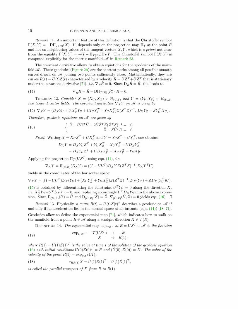
The covariant derivative allows to obtain equations for the geodesics of the mani-fold M . These geodesics (Figure 2b) are the shortest paths among all possible smoothcurves drawn on M joining two points sufficiently close. Mathematically, they arecurves R(t) = U(t)Z(t) characterized by a velocity R = UZT +UZT that is stationaryunder the covariant derivative [71], i.e. ∇RR = 0. Since DRR = R, this leads to

(14) ∇RR = R−DΠT (R)(R) · R = 0.

Theorem 12. Consider X = (XU , XZ) ∈ H(U,Z) and Y = (YU , YZ) ∈ H(U,Z)

two tangent vector fields. The covariant derivative ∇XY on M is given by

(15) ∇XY = (DXYU +UXTUYU + (XUY

TZ + YUX

TZ )Z(ZTZ)−1, DXYZ −ZY TU XU ).

Therefore, geodesic equations on M are given by

(16)

U + UUT U + 2U ZTZ(ZTZ)−1 = 0

Z − ZUT U = 0.

Proof. Writing X = XUZT + UXT

Z and Y = YUZT + UY TZ , one obtains:

DXY = DXYUZT + YUX

TZ +XUY

TZ + UDXY

TZ

= DXYUZT + UDXY

TZ +XUY

TZ + YUX

TZ .

Applying the projection ΠT (UZT ) using eqn. (11), i.e.

∇XY = Π(U,Z)(DXY ) = ((I − UUT )DXY Z(ZTZ)−1, DXYTU),

yields in the coordinates of the horizontal space:

∇XY = ((I −UUT )DX(YU ) + (XUYTZ + YUX

TZ )Z(ZTZ)−1, DX(YZ) +ZDX(Y TU )U).

(15) is obtained by differentiating the constraint UTYU = 0 along the direction X,i.e. XT

UYU+UTDXYU = 0, and replacing accordingly UTDXYU into the above expres-sion. Since D(U,Z)(U) = U and D(U,Z)(Z) = Z, ∇(U,Z)(U , Z) = 0 yields eqs. (16).

Remark 13. Physically, a curve R(t) = U(t)Z(t)T describes a geodesic on M ifand only if its acceleration lies in the normal space at all instants (eqn. (14)) [18, 71].

Geodesics allow to define the exponential map [71], which indicates how to walk onthe manifold from a point R ∈M along a straight direction X ∈ T (R).

Definition 14. The exponential map expUZT at R = UZT ∈M is the function

(17)expUZT : T (UZT ) → M

X 7→ R(1),

where R(1) = U(1)Z(1)T is the value at time 1 of the solution of the geodesic equation(16) with initial conditions U(0)Z(0)T = R and (U(0), Z(0)) = X. The value of thevelocity of the point R(1) = expUZT (X),

(18) τRR(1)X = U(1)Z(1)T + U(1)Z(1)T ,

is called the parallel transport of X from R to R(1).


3. Curvature and differentiability of the orthogonal projection ontosmooth embedded manifolds. Differentiability results for the orthogonal projec-tion onto smooth embedded manifolds, as presented with tensor notations in [7], arenow centralized and adapted to the present study. The main motivation is that theSVD truncation (section 4) is an example of such orthogonal projection in the partic-ular case of the fixed-rank manifold. Hence, general geometric differentiability resultsfor the projections will transpose directly into a formula for the differential of theapplication mapping a matrix to its best low rank approximation. The same analysiscan be applied to other matrix manifolds to obtain the differential of other algebraicoperations, and even generalized to non-Euclidean ambient spaces, which is the objectof [23]. In this section, the space of l-by-m matrices Ml,m is replaced with a generalfinite dimensional Euclidean space E, and the fixed rank manifold with any givensmooth embedded manifold M ⊂ E.

Definition 15. Let M be a smooth manifold embedded in an Euclidian space E.The orthogonal projection of a point R onto M is defined whenever there is a uniquepoint ΠM (R) ∈M minimizing the Euclidean distance from R to M , i.e.

||R−ΠM (R)|| = infR∈M

||R−R||.

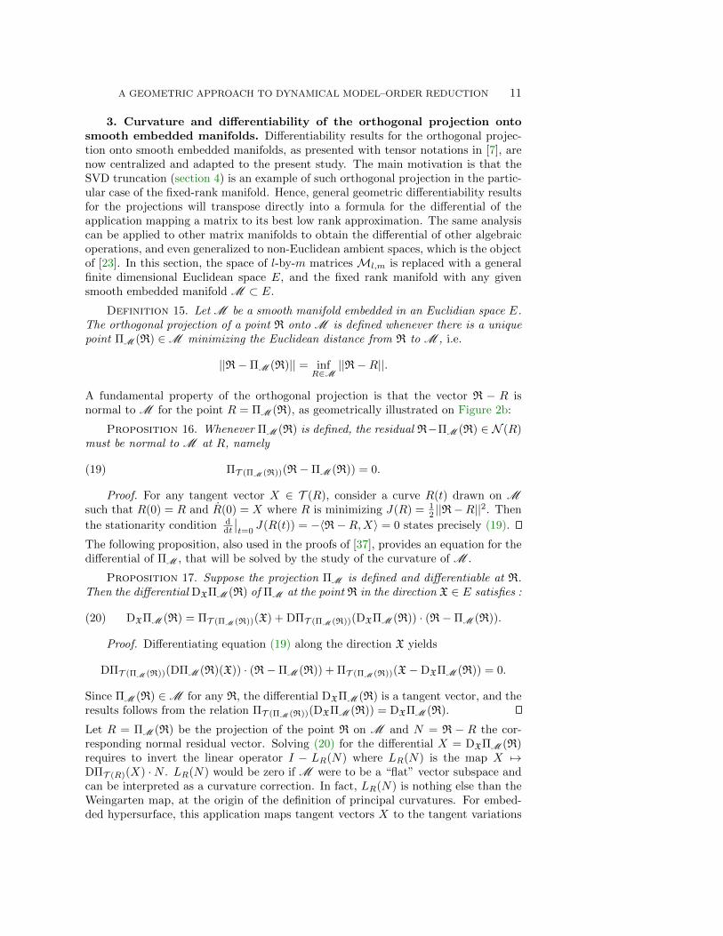
A fundamental property of the orthogonal projection is that the vector R − R isnormal to M for the point R = ΠM (R), as geometrically illustrated on Figure 2b:

Proposition 16. Whenever ΠM (R) is defined, the residual R−ΠM (R) ∈ N (R)must be normal to M at R, namely

(19) ΠT (ΠM (R))(R−ΠM (R)) = 0.

Proof. For any tangent vector X ∈ T (R), consider a curve R(t) drawn on Msuch that R(0) = R and R(0) = X where R is minimizing J(R) = 1

2 ||R−R||2. Then

the stationarity condition ddt

∣∣t=0

J(R(t)) = −〈R−R,X〉 = 0 states precisely (19).

The following proposition, also used in the proofs of [37], provides an equation for thedifferential of ΠM , that will be solved by the study of the curvature of M .

Proposition 17. Suppose the projection ΠM is defined and differentiable at R.Then the differential DXΠM (R) of ΠM at the point R in the direction X ∈ E satisfies :

(20) DXΠM (R) = ΠT (ΠM (R))(X) + DΠT (ΠM (R))(DXΠM (R)) · (R−ΠM (R)).

Proof. Differentiating equation (19) along the direction X yields

DΠT (ΠM (R))(DΠM (R)(X)) · (R−ΠM (R)) + ΠT (ΠM (R))(X−DXΠM (R)) = 0.

Since ΠM (R) ∈M for any R, the differential DXΠM (R) is a tangent vector, and theresults follows from the relation ΠT (ΠM (R))(DXΠM (R)) = DXΠM (R).

Let R = ΠM (R) be the projection of the point R on M and N = R − R the cor-responding normal residual vector. Solving (20) for the differential X = DXΠM (R)requires to invert the linear operator I − LR(N) where LR(N) is the map X 7→DΠT (R)(X) ·N . LR(N) would be zero if M were to be a “flat” vector subspace andcan be interpreted as a curvature correction. In fact, LR(N) is nothing else than theWeingarten map, at the origin of the definition of principal curvatures. For embed-ded hypersurface, this application maps tangent vectors X to the tangent variations


−DXN of the unit normal vector field N , and the eigenvalues and eigenvectors of thissymmetric endomorphism define the principal curvatures and directions of the hyper-surface ([71], Vol. 2). For general smooth embedded sub-manifolds, a Weingartenmap is defined for every possible normal direction [68, 7, 4, 2].

Definition 18 (Weingarten map). For any point R ∈M , tangent and normalvector fields X,Y ∈ T (R) and N ∈ N (R) defined on a neighborhood of R, the followingrelation, called Weingarten identity holds:

(21) 〈ΠT (R)(DXN), Y 〉 = 〈N,Γ(X,Y )〉.

Also, the tangent variations ΠT (R)(DXN) depend only on the value of the normalvector field N at R as it can be seen from the identity

(22) DΠT (R)(X) ·N = −ΠT (R)(DXN).

The applicationLR(N) : T (R) → T (R)

X 7→ DΠT (R)(X) ·N,is therefore a symmetric map of the tangent space into itself and is called the Wein-garten map in the normal direction N . The corresponding eigenvectors and eigenval-ues are respectively called the principal directions and principal curvatures of M inthe normal direction N . The induced symmetric bilinear form on the tangent space,

(23) II(N) : (X,Y ) 7→ −〈N,Γ(X,Y )〉,

is called the second fundamental form in the direction N .

Proof. See [68] or the proof Theorem 5 of [71], vol.3, ch.1.

The differentiability of the projection map for arbitrary sets has been studiedin [81, 1] and more recently in the context of smooth manifolds in [7, 26, 11] withrecent applications in shape optimization [6]. The following theorem reformulatesthese results in the framework of this article. The proof given in Appendix A isessentially a justification that one can indeed invert the operator I −LR(N) by usingits eigendecomposition. Recall that the adherence M is the set of limit points of M .In this paper, the boundary of a manifold is defined as the set ∂M = M \M .

Theorem 19. Let Ω ⊂ E be an open set of E and assume that for any R ∈ Ω,there exists a unique projection ΠM (R) ∈M such that

(24) ||R−ΠM (R)|| = infR∈M

||R−R||,

and that in addition, there is no other projection on the boundary ∂M of M :

(25) ∀R ∈M \M , ||R−R|| > ||R−ΠM (R)||.

For R ∈ Ω, denote κi(N) and Φi the respective eigenvalues and eigenvectors of theWeingarten map LR(N) at R = ΠM (R) with the normal direction N = R−ΠM (R).Then all the principal curvatures satisfy κi(N) < 1 and the projection ΠM is differ-entiable at R. The differential DXΠM (R) at R in the direction X satisfies

(26)

DXΠM (R) =∑κi(N)

1

1− κi(N)〈Φi,X〉Φi

= ΠT (ΠM (R))(X) +∑

κi(N)6=0

κi(N)

1− κi(N)〈Φi,X〉Φi.


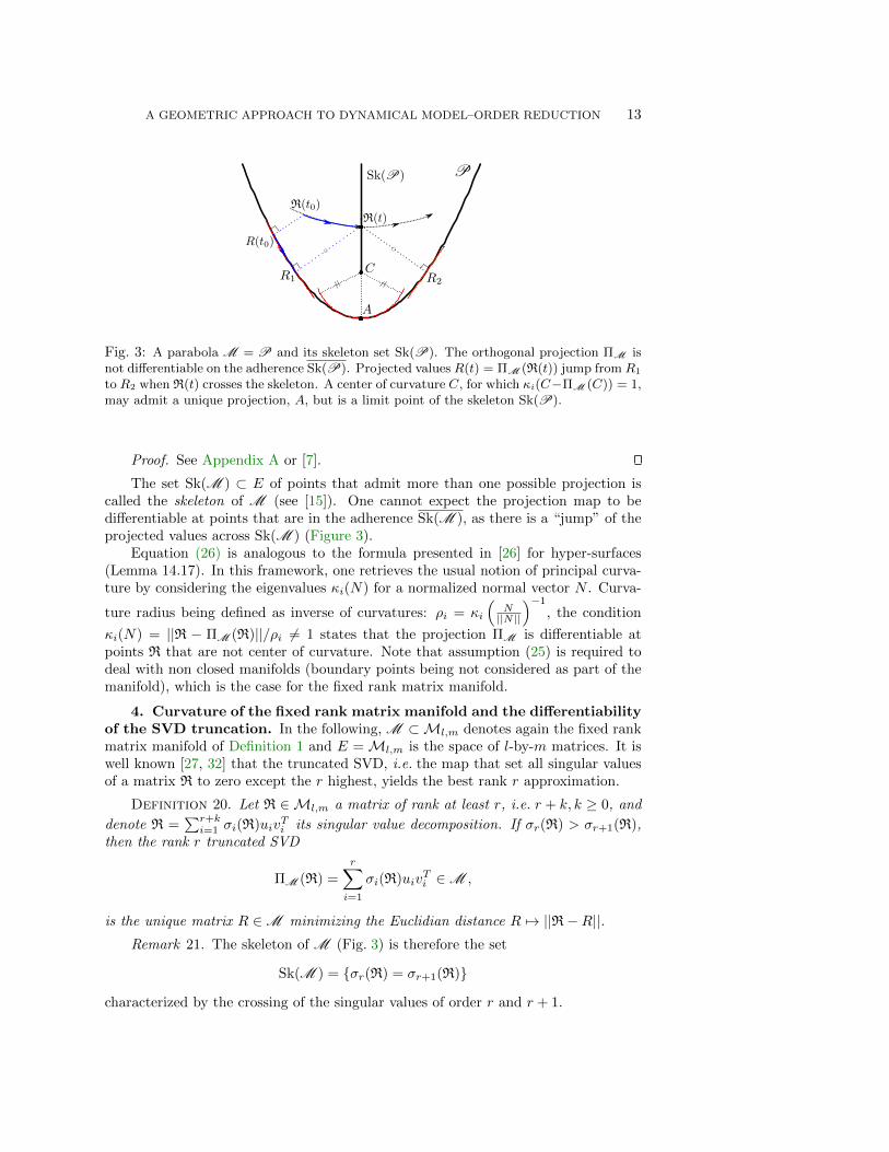
Fig. 3: A parabola M = P and its skeleton set Sk(P). The orthogonal projection ΠM isnot differentiable on the adherence Sk(P). Projected values R(t) = ΠM (R(t)) jump from R1

to R2 when R(t) crosses the skeleton. A center of curvature C, for which κi(C−ΠM (C)) = 1,may admit a unique projection, A, but is a limit point of the skeleton Sk(P).

Proof. See Appendix A or [7].

The set Sk(M ) ⊂ E of points that admit more than one possible projection iscalled the skeleton of M (see [15]). One cannot expect the projection map to bedifferentiable at points that are in the adherence Sk(M ), as there is a “jump” of theprojected values across Sk(M ) (Figure 3).

Equation (26) is analogous to the formula presented in [26] for hyper-surfaces(Lemma 14.17). In this framework, one retrieves the usual notion of principal curva-ture by considering the eigenvalues κi(N) for a normalized normal vector N . Curva-

ture radius being defined as inverse of curvatures: ρi = κi

(N||N ||

)−1

, the condition

κi(N) = ||R − ΠM (R)||/ρi 6= 1 states that the projection ΠM is differentiable atpoints R that are not center of curvature. Note that assumption (25) is required todeal with non closed manifolds (boundary points being not considered as part of themanifold), which is the case for the fixed rank matrix manifold.

4. Curvature of the fixed rank matrix manifold and the differentiabilityof the SVD truncation. In the following, M ⊂Ml,m denotes again the fixed rankmatrix manifold of Definition 1 and E =Ml,m is the space of l-by-m matrices. It iswell known [27, 32] that the truncated SVD, i.e. the map that set all singular valuesof a matrix R to zero except the r highest, yields the best rank r approximation.

Definition 20. Let R ∈ Ml,m a matrix of rank at least r, i.e. r + k, k ≥ 0, and

denote R =∑r+ki=1 σi(R)uiv

Ti its singular value decomposition. If σr(R) > σr+1(R),

then the rank r truncated SVD

ΠM (R) =

r∑i=1

σi(R)uivTi ∈M ,

is the unique matrix R ∈M minimizing the Euclidian distance R 7→ ||R−R||.Remark 21. The skeleton of M (Fig. 3) is therefore the set

Sk(M ) = σr(R) = σr+1(R)

characterized by the crossing of the singular values of order r and r + 1.


In the following, the Weingarten map for the fixed rank manifold is derived. Notethat its expression has been previously found by [4] under the form of equation (31)below.

Proposition 22. The Weingarten map LR(N) of the fixed rank manifold M inthe normal direction N ∈ N (R) is the application:

(27)LR(N) : H(U,Z) −→ H(U,Z)

(XU , XZ) 7−→ (NXZ(ZTZ)−1, NTXU ).

Or, denoting R =∑ri=1 σiuiv

Ti and N =

∑kj=1 σr+jur+jv

Tr+j as in Proposition 9,

this can be rewritten more explicitly as

(28) ∀X ∈ T (R), LR(N)X =∑

1≤i≤r1≤j≤k

σr+jσi

[uiv

Ti X

Tur+jvTr+j + ur+jv

Tr+jX

TuivTi

].

The second fundamental form is given by:

(29) II : (X,Y ) 7→ 〈X,LR(N)(Y )〉 = Tr((XUYTZ + YUX

TZ )TN).

Proof. Differentiating (11) along the tangent direction X = (XU , XZ) ∈ H(U,Z),and using the relations UTN = 0 and NZ = 0, yields

(30) LR(N)X = UXTUN +NXZ(ZTZ)−1ZT .

The normality of N implies that (NXZ(ZTZ)−1, NTXU ) is a vector of the horizontalspace and therefore equation (27) follows. Eqn. (30) can be rewritten as

(31) LR(N)X = U(ZTZ)−1ZTXTN +NXTU(ZTZ)−1ZT ,

by expressing XU = (I − UUT )XZ(ZTZ)−1 and XZ = XTU in terms of X (eqn.(11)), from which is derived eqn. (28) by introducing singular vectors (ui), (vi) andsingular values (σi). One obtains(29) by evaluating the scalar product 〈X,LR(N)(Y )〉with the metric g (equation (10)).

Remark 23. The Christoffel symbol is deduced from equations (29) and (23):

(32) Γ(X,Y ) = −(I −ΠT (R))(XUYTZ + YUX

TZ ).

Theorem 24. Consider a point R = UZT =∑ri=1 σiuiv

Ti ∈ M and a normal

vector N =∑kj=1 σr+jur+jv

Tr+j ∈ N (R) (no ordering of the singular values is as-

sumed). At R and in the direction N , there are 2kr non-zero principal curvatures

κ±i,j(N) = ±σr+jσi

,

for all possible combinations of non-zero singular values σr+j , σi for 1 ≤ i ≤ r and1 ≤ j ≤ k. The normalized corresponding principal directions are the tangent vectors

(33) Φ±i,r+j =1√2

(ur+jvTi ± uivTr+j).

The other principal curvatures are null and associated with the principal subspace

Ker(LR(N)) = span(uivT )1≤i≤r|Nv = 0 ⊕ span(uvTi )1≤i≤r|uTN = uTU = 0.


Proof. From (28), it is clear that LR(N)Φ±i,r+j = κ±i,r+j(N)Φ±i,r+j . In addition,

Φ±i,r+j is indeed a tangent vector as one can write Φ±i,r+j = XUZT ± UXT

Z with:

(XU , XZ) =1√

2σr+jσi(Nvr+ju

Ti U,N

Tur+jvTi Z).

Therefore (Φ±i,r+j) is a family of 2kr independent eigenvectors. Then it is easy to

check that span(uivT )1≤i≤r|Nv = 0 and span(uvTi )1≤i≤r|uTN = uTU = 0 arenull eigenspaces of respective dimension (m−k)r and (l−k−r)r. The total dimensionobtained is (m−k)r+(l−k−r)r+2kr = mr+ lr−r2, implying that the full spectraldecomposition has been characterized.

This theorem shows that the maximal curvature of M (for normalized normal direc-tions ||N || = 1) is σr(R)−1 and hence diverges as the smallest singular value goes to 0.This fact confirms what is visible on Figure 1: the manifold M can be seen as a col-lection of cones or as a multidimensional spiral, whose axes are the lower dimensionalmanifolds of matrices of rank strictly less than r. Applying directly the formula (26)of Theorem 19, one obtains an explicit expression for the differential of the truncatedSVD:

Theorem 25. Consider R ∈ Ml,m with rank greater than r and denote R =∑r+ki=1 σiuiv

Ti its SVD decomposition, where the singular values are ordered decreas-

ingly: σ1 ≥ σ2 ≥ . . . ≥ σr+k. Suppose that the orthogonal projection ΠM (R) = UZT

of R onto M is uniquely defined, that is σr > σr+1. Then ΠM , the truncated SVD oforder r, is differentiable at R and the differential DXΠ(R) in a direction X ∈ Ml,m

is given by the formula

(34) DXΠM (R) = ΠT (ΠM (R))(X)

+∑

1≤i≤r1≤j≤k

[σr+j

σi − σr+j〈X,Φ+

i,r+j〉Φ+i,r+j −

σr+jσi + σr+j

〈X,Φ−i,r+j〉Φ−i,r+j

],

where Φ±i,r+j are the principal directions of equation (33). More explicitly,

(35) DXΠM (R) = (I − UUT )XZ(ZTZ)−1ZT + UUTX

+∑

1≤i≤r1≤j≤k

σr+jσ2i − σ2

r+j

[(σiuTr+jXvi + σr+ju

Ti Xvr+j)ur+jv

Ti

+ (σr+juTr+jXvi + σiu

Ti Xvr+j)uiv

Tr+j ].

Proof. The set R ∈Ml,m, σr+1(R) > σr(R) is open by continuity of the singu-lar values, therefore condition (24) of Theorem 19 is fulfilled. The boundary M \Mis the set of matrices of rank strictly lower than r, hence condition (25) is also ful-filled. Equation (34) follows by replacing κi(N) and Φi in (26) by the correspondingcurvature eigenvalues ±σr+j

σiand eigenvectors Φ±i,r+j of Theorem 24.

Remark 26. Dehaene [14] and Dieci and Eirola [17] have previously derived formu-las for the time derivative of singular values and singular vectors of a smoothly varyingmatrix. One can also certainly use these results to find formula (35) by differentiatingsingular values (σi) and singular vectors (ui), (vi) separately in

∑ri=1 σiuiv

Ti . In the

present work, the proof of Theorem 25 does not require singular values to remainsimple, and formula (34) is obtained directly from its geometric interpretation.


5. The Dynamically Orthogonal Approximation. The above results arenow utilized for model order reduction. Following the introduction, the DO approx-imation is defined to be the dynamical system obtained by replacing the vector fieldL(t, ·) with its tangent projection on the manifold. (Figure 2b).

Definition 27. The maximal solution in time of the reduced dynamical systemon M ,

(36)

R = ΠT (R)(L(t, R))R(0) = ΠM (R(0)),

is called the Dynamically Orthogonal (DO) approximation of (2). The solutionR(t) = U(t)ZT (t) is governed by a dynamical system for the mode matrix U andthe coefficient matrix Z such that (U , Z) ∈ H(U,Z) satisfies the dynamically orthogo-

nal condition UT U = 0 at every instant:

(37)

U = (I − UUT )L(t, UZT )Z(ZTZ)−1

Z = L(t, UZT )TUU(0)Z(0)T = ΠM (R(0)).

Remark 28. Equations (37) are exactly those presented as DO equations in [64,63]. With the notation of (1) and (3), using 〈· , · 〉 to denote the continuous dotproduct operator (an integral over the spatial domain) and E the expectation, theywere written as the following set of coupled stochastic PDEs:

(38)

∂tζi = 〈L (t,uDO;ω),ui〉

r∑j=1

E[ζiζj ]∂tuj = E

ζiL (t,uDO;ω)−

r∑j=1

〈L (t,uDO;ω),uj〉uj

.

However, when dealing with infinite dimensional Hilbert spaces, the vector space ofsolutions of (1) depends on the PDEs, which complicates the derivation of a generaltheory for (38). Considering the DO approximation as a computational method forevolving low rank matrices relaxes these issues through the finite-dimensional setting.

Remark 29. One can relate (36) to projected dynamical systems encountered inoptimization [53], where the manifold M is replaced with a compact convex set.

In the following, two justifications of the accuracy of this approximation are given.First, the DO approximation is shown to be the continuous limit of a scheme thatwould truncate the SVD of the full matrix solution after each time step, and henceis instantaneously optimal among any other possible model order reduced system.Then, its dynamics is compared to that of the best low rank approximation, yieldingerror bounds on global integration times. The efficiency of the DO approach in thecontext of the discretization of a stochastic PDE is not discussed here. These pointsare examined in [22] and in references cited therein.

5.1. The DO system applies instantaneously the truncated SVD. Thisparagraph details first a “computational” interpretation of the DO approximation.Consider the temporal integration of the dynamical system (2) over (tn, tn+1),

(39) Rn+1 = Rn + ∆tL(tn,Rn,∆t),


where L(t,R,∆t) denotes the full-space integral L(t,R,∆t) = 1∆t

∫ t+∆t

tL(s,R(s))ds

for the exact integration or the increment function [28] for a numerical integra-tion. Examples of the latter include L(t,R,∆t) = L(t,R) for forward Euler andL(t,R,∆t) = L(t+ ∆t/2,R+ ∆t/2L(t,R)) for a second-order Runge-Kutta scheme.Assume that the solution Rn at time tn is well approximated by a rank r matrix Rn.A natural way to estimate the best rank r approximation ΠM (Rn+1) at the next timestep is then to set

(40)

Rn+1 = ΠM (Rn + ∆tL(t, Rn,∆t))

R0 = ΠM (R(0)).

Such a numerical scheme uses the truncated SVD, ΠM , to remove after each timestep of the initial time-integration (39) the optimal amount of information requiredto constrain the rank of the solution. A data-driven adaptive version of this approachwas for example used in [42, 43]. One can then look for a dynamical system for which(40) would be a temporal discretization. One then finds that, for any rank r matrixR ∈M ,

(41)ΠM (R+ ∆tL(t, R,∆t))−R

∆t−→

∆t→0DL(t,R,0)ΠM (R) = ΠT (R)(L(t, R))

holds true since the curvature term depending on N = R − ΠM (R) = 0 vanishesin (26), and L(t, R, 0) = L(t, R) by consistency of the time marching with the exactintegration (39) [28]. This implies, under sufficient regularity condition on L, thatthe continuous limit of the scheme (40) is the DO dynamical system (36).

Theorem 30. Assume that the DO solution (36) is defined on a time interval[0, T ] discretized with NT time steps ∆t = T/NT and denote tn = n∆t. ConsiderRn the sequence obtained from the class of schemes (40). Assume that L is Lipschitzcontinuous, that is there exists a constant K such that

(42) ∀t ∈ [0, T ], ∀A,B ∈Ml,m, ||L(t, A)− L(t, B)|| ≤ K||A−B||.

Then the sequence Rn converges uniformly to the DO solution R(t) in the followingsense:

sup0≤n≤NT

||Rn −R(tn)|| −→∆t→0

0

Proof. It is sufficient to check that the scheme (40) is both consistent and stable(see [28]). Denote Φ the increment function of the scheme (40):

(43) Φ(t, R,∆t) =ΠM (R+ ∆tL(t, R,∆t))−R

∆t=

1

∆t

∫ 1

0

d

dτΠM (g(R, t, τ,∆t))dτ

with g(R, t, τ,∆t) = R + τ∆tL(t, R,∆t). Consider a compact neighborhood U ofMl,m containing the trajectory R(t) on the interval [0, T ] and sufficiently thin suchthat U does not intersect the skeleton of M . In particular, ΠM is differentiablewith respect to R on the compact neighborhood U , hence Lipschitz continuous. Theconsistency of (40) and continuity of Φ on [0, T ]×U ×R follows from (41). For usualtime marching schemes (e.g. Runge Kutta), the Lipschitz condition (42) also holds forthe map R 7→ L(t, R,∆t). Therefore it Φ is also Lipschitz continuous with respect toR on U by composition. This is a sufficient stability condition.


As such, the DO approximation can be interpreted as the dynamical system thatapplies instantaneously the truncated SVD to constrain the rank of the solution.Therefore, other reduced order models of the form (4) are characterized by largererrors on short integration times for solutions whose initial value lies on M .

Remark 31. Other dynamical systems that perform instantaneous matrix oper-ations have been derived in [10, 70], and in [14] (e.g. Lemma 3.4 and Corollary 3.5)or [17] (sections 2.1 and 2.3.) for tracking the full SVD or QR decomposition. Con-tinuous SVD has been combined with adaptive Kalman filtering in uncertainty quan-tification to continuously adapt the dominant subspace supporting the stochastic so-lution [42, 43, 41]. All of these results utilized the instantaneous truncated SVDconcept and formed the computational basis of the continuous DO dynamical system.In fact, the dominant singular vectors of state transition matrices and other opera-tors have found varied applications in atmospheric and ocean sciences for some time[19, 20, 56, 33, 45, 51, 35, 16].

5.2. The DO approximation is close to the dynamics of the best lowrank approximation of the original solution. Ideally, a model order reduced so-lution R(t) would coincide at all times with the best rank r approximation ΠM (R(t)),so as to keep the error ||R(t)−R(t)|| minimal. However, ΠM (R(t)) is not the solutionof a reduced system of the form (4) as its time derivative depends on the knowledgeof the true solution R in the full space Ml,m. Indeed, formula (35) for the differen-tial of the SVD yields the following system of ODEs for the evolution of modes andcoefficients of the best rank−r approximation ΠM (R(t)):(44)

U = (I − UUT )RZ(ZTZ)−1

+

∑1≤i≤r1≤j≤k

σr+jσ2i − σ2

r+j

(σiuTr+jRvi + σr+ju

Ti Rvr+j)ur+jv

Ti

Z(ZTZ)−1

Z = RTU +

∑1≤i≤r1≤j≤k

σr+jσ2i − σ2

r+j

(σr+juTr+jRvi + σiu

Ti Rvr+j)vr+ju

Ti

U,where the (time-dependent) SVD of R(t) at the time t is

∑r+ki=1 σiuiv

Ti with k =

min(m, l) (allowing possibly σr+j = 0 for 1 ≤ j ≤ k). One therefore sees from thisbest rank−r governing differential (44) that its reduced DO system (36) is obtained by(i) replacing the derivative R = L(t,R) with the approximation L(t, R) (first terms ineach of the right-hand sides of (44)), and (ii) neglecting the dynamics corresponding tothe interactions between the low-rank−r approximation (singular values and vectorsof order 1 ≤ i ≤ r) and the neglected normal component (singular values and vectorsof order r+ j for 1 ≤ j ≤ k). These interactions are the last summation terms in eachright-hand sides of (44). Estimating these interactions in all generality would require,in addition to the knowledge of a rank r approximation R ' ΠM (R), either externalobservations [43] or closure models [76], so as to estimate the otherwise neglected

normal component R−ΠM (R) =∑kj=1 σr+jur+jv

Tr+j .

Comparing the dynamics (37) of the DO approximation to that of the governingdifferential (44) of the best low rank−r approximation, a bound for the growth of theDO error is now obtained.


Theorem 32. Assume that both the original solution R(t) ∈Ml,m (eqn. (2)) andits DO approximation R(t) (eqn. (36)) are defined on a time interval [0, T ] and thatthe following conditions hold:

1. L is Lipschitz continuous, i.e. equation (42) holds.2. The original (true) solution R(t) remains close to the low rank manifold M ,

in the sense that R(t) does not cross the skeleton of M on [0, T ], i.e. there isno crossing of the singular value of order r:

∀t ∈ [0, T ], σr(R(t)) > σr+1(R(t)).

Then, the error of the DO approximation R(t) (eqn. (36)) remains controlled by thebest approximation error ||R−ΠM (R(t))|| on [0, T ]:

(45) ∀t ∈ [0, T ], ||R(t)−ΠM (R(t))|| ≤∫ t

0

||R(s)−ΠM (R(s))||(K +

||L(s,R(s))||σr(R(s))− σr+1(R(s))

)eη(t−s)ds,

where η is the constant

(46) η = K + supt∈[0,T ]

2

σr(R(t))||L(t,R(t))||.

Proof. A proof is given in Appendix B.

This statement improves the result expressed in [37] (Theorem 5.1), since no assump-tion is made on the smallness of the best approximation error ||R − ΠM (R)||, noron the boundedness of ||R − ΠM (R)||. Theorem 32 also highlights two sufficientconditions for the error committed by the DO approximation to remain small :

Condition 1. The discrete operator L must not be too sensitive to the errorR(t)−R(t), namely the Lipschitz constant K must be small. This error is commonlyencountered by any approximation made for evaluating the operator of a dynamicalsystem (as a consequence of Gronwall’s lemma [29]). The Lipschitz constant K alsoquantifies how fast the vector field L may deviate from its values when getting awayfrom the low rank manifold M .

Condition 2. Independently of the choice of the reduced order model, the solu-tion of the initial system (2), R(t), must remain close to the manifold M , or in otherwords, must remain far from the skeleton Sk(M ) of M . As visible on Figure 3, thebest rank r approximation ΠM (R) of R exhibits a jump when R crosses the skeleton,i.e. when σr(R) = σr+1(R) occurs. At that point, the discontinuity of ΠM (R(t))cannot be tracked by the DO or any other smooth dynamical approximation. Con-dition 2 in some sense supersedes the stronger condition of “smallness of the initialtruncation error” of the error analysis of [37]. Indeed, when σr(R) ' σr+1(R) occurs,as observed numerically in [52], the DO solution may then diverge sharply from theSVD truncation. From the point of view of model order reduction, the resulting errorcan be related to the evolution of the residual R−ΠM (R) that is not accounted forby the reduced order model. When the crossing of singular values occurs, neglectedmodes in the approximation (3) become “dominant”, but cannot be captured by areduced order model that has evolved only the first modes initially dominant. Insuch cases, one has to restart the simulations from the initial conditions with a largersubspace size or the size of the DO subspace has to be increased and corrections ap-plied from external information. The latter learning of the subspace can be done from


measurements or from additional Monte-Carlo simulations and breeding of the bestlow-rank−r approximation [43, 35, 65].

Last, it should be noted that the growth rate η (equation (46)) of the errorincreases as the evolved trajectory becomes close to be singular, i.e. when σr(R(t))goes to zero. This growth rate comes mathematically from the Gronwall estimatesof the proofs, and is intuitively related to the fact the tangent projection ΠT in (36)is applied at the location of the DO solution R(t) instead of the one of the bestapproximation ΠM (R(t)). If the evolved trajectory is close to be singular, the localcurvature of M experienced by the DO solution R(t) and the best approximationΠM (R(t)) is high. Therefore the tangent spaces T (R(t)) and T (ΠM (R(t))) may beoriented very differently because of this curvature, resulting in increased error whenapproximating the tangent projection operator ΠT (ΠM (R(t))) by ΠT (R(t)) in the DOsystem (36).

Remark 33. Theorems 30 and 32 may be generalized in a straightforward mannerto the case of any smooth embedded manifolds M ⊂ E (Theorem 2.5 and 2.6 in [21]).

6. Optimization on the fixed rank matrix manifold for tracking thebest low rank approximation. This section applies the framework of Riemannianmatrix optimization [18, 2] as an alternative approach to the direct tracking of thetruncated SVD of a time-dependent matrix R(t) ∈ Ml,m. At the end, we provide aremark (Remark 38) linking the two approaches within the context of the DO system.

Consider a given (full-rank) matrix R ∈Ml,m and recall that ΠM (R), when it isnon-ambiguously defined, is the unique minimizer of the distance functional

(47)J : M −→ R

R 7−→ 12 ||R−R||2.

Riemannian optimization algorithms, namely gradient descents and Newton methodson the fixed rank manifold M , are now used to provide alternative ways to more stan-dard direct algebraic algorithms [27] for evaluating the truncated SVD ΠM (R). Suchoptimizations can be useful to dynamically update the best low rank approximationof a time dependent matrix R(t): this is because for a sufficiently small time step∆t, R(t) = ΠM (R(t)) is expected to be close to R(t+ ∆t) = ΠM (R(t+ ∆t)), henceΠM (R(t)) provides a good initial guess for the minimization of R 7→ ||R(t+∆t)−R||.The minimization of the distance functional J has already been considered in the ma-trix optimization community [3, 75, 50] that derived gradient descent and Newtonmethods on the fixed rank manifold, but not in the case of the metric inherited fromthe ambient spaceMl,m (eqn. (10)), which is done in what follows. As a benefit of this“extrinsic” approach already noticed in [4], the covariant Hessian of J relates directlyto the Weingarten map at critical points: this will allow obtaining the convergence ofthe gradient descent for almost every initial data (Proposition 36).

Ingredients required for the minimization of J on the manifold M are first derived,namely the covariant gradient and Hessian. As reviewed in [18], usual optimizationalgorithms such as gradient and Newton methods can be straightforwardly adapted tomatrix manifolds. The differences with their Euclidean counterparts is that: (i) usualgradient and Hessians must be replaced by their covariant equivalents; (ii) one needs tofollow geodesics instead of straight lines to move on the manifold; and, (iii) directionsfollowed at the previous time steps, needed for example in the conjugate gradientmethod, must be transported to the current location (equation (18)). Covariantgradient and Hessian are recalled in the following definition (for details, see [3], chapter5).


Definition 34. Let J be a smooth function defined on M and R ∈ M . Thecovariant gradient of J at R is the unique vector ∇J ∈ T (R) such that

∀X ∈ T (R), J(expR(tX)) = J(R) + t〈∇J,X〉+ o(t).

The covariant Hessian HJ of J at R is the linear map on T (R) defined by

HJ(X) = ∇X∇J,

and the following second order Taylor approximation of J holds:

J(expR(tX)) = J(R) + t〈∇J,X〉+t2

2〈X,HJ(X)〉+ o(t2).

The following proposition (see [4]) explains how these quantities are related to theusual gradient and Hessian, so that they become accessible for computations.

Proposition 35. Let J be a smooth function defined in the ambient space Ml,m

and denote DJ and D2J its respective Euclidean gradient and Hessian. Then thecovariant gradient and Hessian are given by

(48) ∇J = ΠT (R)(DJ),

(49) HJ(X) = ΠT (R)(D2J(X)) + DΠT (R)(X) ·

[(I −ΠT (R))(DJ)

].

Applying directly Proposition 35, the gradient and the Hessian of J at R = UZT ∈Mare given by:

(50) ∇J = ((I − UUT )(UZT −R)Z(ZTZ)−1, (UZT −R)TU),

(51)HJ : H(U,Z) → H(U,Z)(

XU

XZ

)7→

(XU −NUZT (R)XZ(ZTZ)−1

XZ −NUZT (R)TXU

),

where NUZT (R) = (I − ΠT (UZT ))(R − UZT ) = (I − UUT )R(I − Z(ZTZ)−1ZT ) isthe orthogonal projection of R−R onto the normal space. The Newton direction Xis found by solving the linear system HJ(X) = −∇J(R), that reduces to

XUA+BXZ = EBTXU +XZ = F,

with A = (ZTZ), B = −NUZT (R), E = (I − UUT )RZ and F = −Z + RTU . Thisrequires to solve the Sylvester equation XUA − BBTXU = E − BF for XU , thatcan be done in theory by using standard techniques [36], before computing XZ fromXZ = F −BTXU .

It is now proven that the distance function J may admit several critical points,but a unique local, hence global, minimum on M . As a consequence, saddle pointsof J are unstable equilibrium solutions of the gradient flow R = −∇J(R) and henceare expected to be avoided by gradient descent, which will converge in practice to theglobal minimum ΠM (R). This “almost surely” convergence guarantee for the gradi-ent descent may be compared to probabilistic analyses investigated in more generalcontexts [59, 77]. Our result also shows that one cannot expect the Newton method toconverge for initial guesses that are far from the optimal. Indeed, this method seeksa zero of the gradient ∇J rather than a true minimum, and hence may converge oroscillate around several of the saddle points of the objective function.


0 10 20 30 40

Iteration

1400

1450

1500

1550

1600

1650

J

Objective function

Gradient flow

Conjugated gradient descent

0 20 40 60 80 100

Iteration

10-15

10-10

10-5

100

105

dR

t

Increments

Newton

Conjugated gradient

Gradient flow

Fig. 4: Convergence curves of optimization algorithms for minimizing the distance functionJ (equation (47)). Newton does not converge to the global minimum and hence is notrepresented on the left curve.

Proposition 36. Consider R ∈ Ml,m such that its projection onto M is welldefined, that is σr(R) > σr+1(R). Then the distance function J to R (eqn. (47))admits no other local minima than ΠM (R). In other words, for almost any initialrank r matrix U(0)Z(0)T , the solution U(t)Z(t)T of the gradient flow

(52)

U = (I − UUT )RZ(ZTZ)1

Z = RTU − Z

converges to ΠM (R), the rank r truncated SVD of R.

Proof. It is known from Proposition 16 that the points R for which ∇J vanishesare such that DJ = R − R ∈ N (R) is a normal vector. Since in addition D2J = I,Proposition 35 yields the identity

∀X ∈ T (R), 〈HJ(X), X〉 = 〈X,X〉 − 〈DΠT (R)(X) ·N,X〉= ||X||2 − 〈LR(N)(X), X〉,

where N = −(I − ΠT (R))(DJ) = −DJ = R − R ∈ N (R), since ∇J = ΠT (R)(DJ)

vanishes at R. Let R =∑r+ki=1 σi(R)uiv

Ti be the SVD of R. For R−R to be a normal

vector, R must necessary be of the form R =∑i∈A σiuiv

Ti where A is a subset of r

indices 1 ≤ i ≤ r + k. Then the minimum eigenvalue of the Hessian H is 1 − σ1(N)σr(R) ,

which is positive if and only if σr(R) > σ1(N). This happens only for R = ΠM (R).

Remark 37. The reader is referred to [34] for details regarding the convergencealmost surely of sufficiently smooth gradient flows towards the unique minimizer of afunction (Morse theory).

On Figure 4, a matrix R ∈ Ml,m with m = 100 and l = 150 is considered, withsingular values chosen to be equally spaced in the interval [1, 10]. Three optimiza-tion algorithms detailed in [18] (gradient descent with fixed step, conjugate gradientdescent, and Newton method) are implemented to find the best rank r = 5 approxima-tion of R, with a random initialization. Convergence curves are plotted on Figure 4:linear and quadratic rates characteristic of respectively gradient and Newton methodsare obtained. As expected from Proposition 36, gradient descents globally convergeto the truncated SVD, while Newton iterations may be attracted to any saddle point.


Remark 38. The above gradient descent and Newton methods can be combinedwith previously-derived numerical schemes for the time-integrated DO eqs. (40). Oneclass of schemes consists of discretizing the ODEs (37) in time, as in [64, 73, 52, 37].Another follows (40) directly and aims to compute the SVD truncation ΠM (R) ofR = UZT + ∆tL(t, UZT ,∆t), where the increment function can be that of Euler orof higher-order explicit time marching (of course, the total rank of this R dependson the dynamics and numerical scheme, and can be greater than r). Examining theexpression of the gradient of J (eqn. (50)), one time-step of the above schemes can beinterpreted as one gradient descent step for minimizing the functional J . Therefore,optimization algorithms on the Riemannian manifold M can be combined with suchDO time-stepping schemes, as further investigated in [22]. A key advantage of suchoptimization is the capability of altering the rank r of the dynamical approximationover a time step or stage (e.g. a rank p > r approximation can be used in the tar-get cost functional J). These strategies may also be utilized for the computation ofnonlinear singular vectors [74] or for continuous dominant subspace estimation [41].Finally, it can also be combined with adaptive learning schemes [43, 45, 65] which usesystem measurements and/or Monte-Carlo breeding nonlinear simulations to estimatethe missing fastest growing modes. Such additional information can then correct thepredictor of the SVD of R(t+ ∆t) in directions orthogonal to the discrete DO incre-ments and essentially increase the subspace size, e.g. when the estimates of σr+1(R(t))become close to these of σr(R(t)).

7. Conclusion. A geometric approach was developed for dynamical model-orderreduction, through the analysis of the embedded geometry of the fixed rank manifoldM . The extrinsic curvatures of matrix manifolds were studied and geodesic equationsobtained. The relationships among these notions and the differential of the orthogonalprojection of the original system dynamics onto the tangent spaces of the manifoldwere derived and linked to the DO approximation. These geometric results allowed toderive the differential of the truncated SVD interpreted as an orthogonal projectiononto the fixed rank matrix manifold. The DO approximation, with its instantaneousapplication of the SVD truncation of the stochastic/parametric dynamics, was shownto be the natural dynamical reduced-order model that is optimal on small integrationtimes among all other reduced-order models that evaluate the operator of the full-space dynamics exclusively onto low rank approximations. Additionally, the explicitdynamical system satisfied by the best low rank approximation was derived and usedto sharpen the error analysis of the DO approximation.

The DO method was related to Riemannian matrix optimization, for which gra-dient descent methods were applied and shown capable of adaptively tracking thebest low rank approximation of dynamic matrices. This may prove beneficial in theintegration of the time stepping of the DO approximation. Such approaches, in con-trast with classic numerical integrations of the governing differential equations for theDO modes and their coefficients, open new future avenues for efficient DO numericalschemes. In general, there are now many promising directions for developing new,efficient, dynamic reduced-order methods, based on the geometry and shape of thefull-space dynamics. Opportunities abound over a wide range of needs and applica-tions of uncertainty quantification and dynamical system analyses and optimizationin oceanic and atmospheric sciences, thermal-fluid sciences and engineering, electricalengineering, and chemical and biological sciences and engineering.

Acknowledgments. We thank the members of the MSEAS group at MIT aswell as Camille Gillot, Christophe Zhang, and Saviz Mowlavi for insightful discussions


related to this topic. We are grateful to the Office of Naval Research for support undergrants N00014-14-1-0725 (Bays-DA) and N00014-14-1-0476 (Science of Autonomy –LEARNS) to the Massachusetts Institute of Technology.

Appendix A. Proof of Theorem 19.

Lemma 39. Let Ω be an open set over which the projection ΠM is uniquely definedby eqn. (24) and such that condition (25) holds. Then ΠM is continuous on Ω.

Proof. Consider a sequence Rn converging in E to R and denote ΠM (Rn) thecorresponding projections. Let ε > 0 be a real such that ∀n ≥ 0, ||Rn−R|| < ε. Since

||ΠM (Rn)−R|| ≤ ||ΠM (Rn)−Rn||+ ||Rn −R||≤ ||Rn −ΠM (R)||+ ||Rn −R||≤ 2ε+ ||R−ΠM (R)||,

the sequence ΠM (Rn) is bounded. Denote R ∈ M a limit point of this sequence.Passing to the limit the inequality ||Rn − ΠM (Rn)|| ≤ ||Rn − ΠM (R)||, one obtains||R − R|| ≤ ||R − ΠM (R)||. The uniqueness of the projection, and the fact thatthere is no R ∈M \M satisfying this inequality, shows that R = ΠM (R). Since thebounded sequence (ΠM (Rn)) has a unique limit point, one deduces the convergenceΠM (Rn)→ ΠM (R) and hence the continuity of the projection map at R.

Lemma 40. At any point R ∈ Ω, any principal curvature κi(N) in the directionN at ΠM (R) must satisfy κi(N) < 1.

Proof. It is shown in Proposition 35 that the covariant Hessian of the distancefunction J(R) = 1

2 ||R− J ||2 at R = ΠM (R) is given by

(53)HJ : T (R) → T (R)

X 7→ X − LR(N)(X),

where N is the normal direction N = R − ΠM (R). Since R = ΠM (R) must be alocal minimum of J , this Hessian must be positive, namely any eigenvalue κi(N) ofthe Weingarten map LR(N) must satisfy 1 − κi(N) ≥ 0. Now, consider s > 1 suchthat R+ sN ∈ Ω and notice that ||R+ sN −ΠM (R)|| = s||N ||. Since

||R+ sN −ΠM (R+ sN)|| ≤ ||R+ sN −ΠM (R)|| = s||N ||,

the uniqueness of the projection in Ω implies that ΠM (R+sN) = R (i.e. the projectionis invariant along orthogonal rays). The linearity of the Weingarten map in N impliesκi(sN) = sκi(N), hence κi(N) ≤ 1

s < 1, which concludes the proof.

Proof of Theorem 19. Consider the function f(R, R) = ΠT (R)(R−R) defined onM ×E. The differential of f with respect to the variable R in a direction X ∈ T (R)at R = ΠM (R) is the application

X 7→ ΠT (R)X −DXΠT (R)(R−R) = (I − LR(N))(X).

Lemma 40 implies that the Jacobian ∂R,Xf has no zero eigenvalue and hence isinvertible. The implicit function theorem ensures the existence of a diffeomorphismφ mapping an open neighborhood ΩE ⊂ E of R to an open neighborhood ΩM ⊂Mof R, such that for any R′ ∈ ΩE , φ(R′) is the unique element of ΩM satisfyingf(R′, φ(R′)) = 0. By continuity of the projection (Lemma 39), one can assume, byreplacing ΩE with the open subset ΩE ∩Π−1

M (ΩM ), that ΠM (ΩE) ⊂ ΩM . Then, the


equality f(R′,ΠM (R′)) = 0 implies by uniqueness: φ(R′) = ΠM (R′). Hence ΠM = φon ΩE , and, in particular, ΠM is differentiable. Finally, for a given X ∈ E, one cannow solve (20) by projection onto the eigenvectors of LR(N) and obtain (26).

Appendix B. Proof of Theorem 32.

Lemma 41. For any R ∈Ml,m satisfying σr(R) > σr+1(R) and X ∈Ml,m :

||DXΠM (R)−ΠT (ΠM (R))X|| ≤σr+1(R)

σr+1(R)− σr(R)||X||.

Proof. This is a consequence of the fact that the maximum eigenvalue in thedecomposition (26) is

maxi,j

σr+j(R)σi(R)

1− σr+j(R)σi(R)

=σr+1(R)

σr(R)− σr+1(R).

The following lemma can be found in [77] and Theorem 2.6.1 in [27].

Lemma 42. For any points R1, R2 ∈M the following estimate holds:

(54) ||ΠT (R1) −ΠT (R2)|| ≤ min

(1,

2

σr(R1)||R1 −R2||

),

where the norm of the left-hand side is the operator norm.

Remark 43. This result from [77] enhances the “curvature estimates” of Lemma4.2. of [37] that allows to have a global bound and hence avoids the smallness as-sumption of the initial truncation error. Note that such a bound always exists atevery points of smooth manifolds (Definition 2.17 of [21]). A purely geometric analy-sis (Lemma 3.1. in [21]) may also be used to yield locally a sharper bound than (54)but with a larger constant 5/2 instead of 2 as a global estimate.

Proof of Theorem 32. Denote R∗(t) = ΠM (R(t)). Since R∗(t) = DRΠM (R(t)),bounding (20) and using (2) and Lemma 41 yields:

||R− R∗|| ≤ ||ΠT (R∗)(L(t,R))−ΠT (R)(L(t, R))||+ σr+1(R)

σr(R)− σr+1(R)||L(t,R)||.

Furthermore, by triangle inequality,

||ΠT (R∗)(L(t,R))−ΠT (R)(L(t, R))|| ≤ ||ΠT (R∗)(L(t,R))−ΠT (R)(L(t,R))||+ ||ΠT (R)(L(t,R))−ΠT (R)(L(t, R∗))||+ ||ΠT (R)(L(t, R∗))−ΠT (R)(L(t, R))||.

The Lemma 42 (first eqn.) and Lipschitz continuity of L (last two eqs.) then imply

||ΠT (R∗)(L(t,R))−ΠT (R)(L(t,R))|| ≤ 2

σr(R∗)||R−R∗|| ||L(t,R)||,

||ΠT (R)(L(t,R))−ΠT (R)(L(t, R∗))|| ≤ K||R−R∗||,||ΠT (R)(L(t, R∗))−ΠT (R)(L(t, R))|| ≤ K||R−R∗||.

Finally, the following inequality is derived, combining all above equations together:

(55) ||R− R∗||

≤(K +

2||L(t,R)||σr(R∗)

)||R−R∗||+

(K +

||L(t,R)||σr(R)− σr+1(R)

)||R−R∗||.

An application of Gronwall’s Lemma (see corollary 4.3. in [29]) yields (45).


REFERENCES

[1] T. Abatzoglou, The metric projection on C2 manifolds in banach spaces, Journal of Approx-imation Theory, 26 (1979), pp. 204–211.

[2] P. Absil, J. Trumpf, R. Mahony, and B. Andrews, All roads lead to Newton: Feasiblesecond-order methods for equality-constrained optimization, tech. report, Citeseer, 2009.

[3] P.-A. Absil, R. Mahony, and R. Sepulchre, Optimization algorithms on matrix manifolds,Princeton University Press, 2009.

[4] P.-A. Absil, R. Mahony, and J. Trumpf, An extrinsic look at the riemannian hessian, inGeometric Science of Information, Springer, 2013, pp. 361–368.

[5] P.-A. Absil and J. Malick, Projection-like retractions on matrix manifolds, SIAM Journalon Optimization, 22 (2012), pp. 135–158.

[6] G. Allaire, C. Dapogny, G. Delgado, and G. Michailidis, Multi-phase structural optimiza-tion via a level set method, ESAIM. Control, Optimisation and Calculus of Variations, 20(2014), p. 576.

[7] L. Ambrosio, Geometric evolution problems, distance function and viscosity solutions,Springer, 2000.

[8] A. Bartel, M. Clemens, M. Gnther, and E. J. W. ter Maten, Scientific Computing inElectrical Engineering, Springer International Publishing, 2016.

[9] P. Benner, S. Gugercin, and K. Willcox, A survey of projection-based model reductionmethods for parametric dynamical systems, SIAM Review, 57 (2015), pp. 483–531.

[10] R. W. Brockett, Dynamical systems that sort lists, diagonalize matrices and solve linearprogramming problems, in Decision and Control, 1988., Proceedings of the 27th IEEEConference on, IEEE, IEEE, 1988, pp. 799–803.

[11] P. Cannarsa and P. Cardaliaguet, Representation of equilibrium solutions to the tableproblem of growing sandpiles, Journal of the European Mathematical Society, 6 (2004),pp. 435–464.

[12] Y. Cao, J. Zhu, I. M. Navon, and Z. Luo, A reduced-order approach to four-dimensionalvariational data assimilation using proper orthogonal decomposition, International Journalfor Numerical Methods in Fluids, 53 (2007), pp. 1571–1583.

[13] P. G. Constantine, Active subspaces: Emerging ideas for dimension reduction in parameterstudies, vol. 2, SIAM, 2015.

[14] J. Dehaene, Continuous-time matrix algorithms systolic algorithms and adaptive neural net-works, (1995).

[15] M. C. Delfour and J.-P. Zolesio, Shapes and geometries: metrics, analysis, differentialcalculus, and optimization, vol. 22, Siam, 2011.

[16] E. P. Diaconescu and R. Laprise, Singular vectors in atmospheric sciences: A review, Earth-Science Reviews, 113 (2012), pp. 161 – 175.

[17] L. Dieci and T. Eirola, On smooth decompositions of matrices, SIAM Journal on MatrixAnalysis and Applications, 20 (1999), pp. 800–819.

[18] A. Edelman, T. A. Arias, and S. T. Smith, The geometry of algorithms with orthogonalityconstraints, SIAM journal on Matrix Analysis and Applications, 20 (1998), pp. 303–353.

[19] B. F. Farrell and P. J. Ioannou, Generalized stability theory. part i: Autonomous operators,Journal of the atmospheric sciences, 53 (1996), pp. 2025–2040.

[20] B. F. Farrell and P. J. Ioannou, Generalized stability theory. part ii: Nonautonomousoperators, Journal of the Atmospheric Sciences, 53 (1996), pp. 2041–2053.

[21] F. Feppon, Riemannian Geometry of Matrix Manifolds for Lagrangian Uncertainty Quantifi-cation of Stochastic Fluid Flows, master’s thesis, Massachusetts Institute of Technology,2017.

[22] F. Feppon and P. F. J. Lermusiaux, Dynamically Orthogonal Numerical Schemes for Effi-cient Stochastic Advection and Lagrangian Transport, Submitted to SIAM Review, (2017).

[23] F. Feppon and P. F. J. Lermusiaux, The Extrinsic Geometry of Continuous Time MatrixAlgorithms, Submitted to SIAM Journal of Matrix Analysis and Applications, (2017).

[24] L. Fortuna, G. Nunnari, and A. Gallo, Model order reduction techniques with applicationsin electrical engineering, Springer Science & Business Media, 2012.

[25] R. G. Ghanem and P. D. Spanos, Stochastic finite elements: a spectral approach, CourierCorporation, 2003.

[26] D. Gilbarg and N. S. Trudinger, Elliptic partial differential equations of second order,springer, 2015.

[27] G. H. Golub and C. F. Van Loan, Matrix computations, vol. 3, JHU Press, 2012.[28] E. Hairer, S. Norsett, and G. Wanner, Solving Ordinary Differential Equations I, Nonstiff

Problems, Section III, 8 (2000).


[29] P. Hartman, Ordinary Differential Equations, Society for Industrial and Applied Mathematics,second ed., 2002.

[30] P. Holmes, J. L. Lumley, and G. Berkooz, Turbulence, coherent structures, dynamicalsystems and symmetry, vol. 36, Cambridge university press, 1998.

[31] R. A. Horn and C. R. Johnson, Topics in matrix analysis, Cambridge Univ. Press Cambridgeetc, 1991.

[32] R. A. Horn and C. R. Johnson, Matrix Analysis, Cambridge University Press (CUP), 2009.[33] B. Hoskins, R. Buizza, and J. Badger, The nature of singular vector growth and structure,

Quarterly Journal of the Royal Meteorological Society, 126 (2000), pp. 1565–1580.[34] J. Jost, Riemannian geometry and geometric analysis, Springer Science & Business Media,

2008.[35] E. Kalnay, Atmospheric modeling, data assimilation and predictability, Cambridge university

press, 2003.[36] P. Kirrinnis, Fast algorithms for the sylvester equation ax- xbt= c, Theoretical Computer

Science, 259 (2001), pp. 623–638.[37] O. Koch and C. Lubich, Dynamical low-rank approximation, SIAM Journal on Matrix Anal-

ysis and Applications, 29 (2007), pp. 434–454.[38] J. N. Kutz, Data-driven modeling & scientific computation: methods for complex systems &

big data, OUP Oxford, 2013.[39] S. Lall, J. E. Marsden, and S. Glavaski, A subspace approach to balanced truncation for

model reduction of nonlinear control systems, International Journal of Robust and Non-linear Control, 12 (2002), pp. 519–535.

[40] T. Lee, F. Wang, and R. Newell, Robust model-order reduction of complex biological pro-cesses, Journal of Process Control, 12 (2002), pp. 807–821.

[41] P. Lermusiaux, Evolving the subspace of the three-dimensional multiscale ocean variability:Massachusetts bay, Journal of Marine Systems, 29 (2001), pp. 385–422.

[42] P. F. Lermusiaux, Error subspace data assimilation methods for ocean field estimation: theory,validation and applications, Harvard University, 1997.

[43] P. F. J. Lermusiaux, Estimation and study of mesoscale variability in the Strait of Sicily,Dynamics of Atmospheres and Oceans, 29 (1999), pp. 255–303.

[44] P. F. J. Lermusiaux, Uncertainty estimation and prediction for interdisciplinary ocean dy-namics, Journal of Computational Physics, 217 (2006), pp. 176–199.

[45] P. F. J. Lermusiaux, Adaptive modeling, adaptive data assimilation and adaptive sampling,Physica D: Nonlinear Phenomena, 230 (2007), pp. 172–196.

[46] P. F. J. Lermusiaux, C.-S. Chiu, G. G. Gawarkiewicz, P. Abbot, A. R. Robinson, R. N.Miller, P. J. Haley, Jr, W. G. Leslie, S. J. Majumdar, A. Pang, and F. Lekien,Quantifying uncertainties in ocean predictions, Oceanography, 19 (2006), pp. 92–105.

[47] B. Lin and D. McLaughlin, Real-time ensemble control with reduced-order modeling, SIAMJournal on Scientific Computing, 36 (2014), pp. B749–B775.

[48] M. Loeve, Probability theory, vol. ii, Graduate texts in mathematics, 46 (1978), pp. 0–387.[49] A. J. Majda, I. Timofeyev, and E. Vanden-Eijnden, Systematic strategies for stochastic

mode reduction in climate, Journal of the Atmospheric Sciences, 60 (2003), pp. 1705–1722.[50] B. Mishra, G. Meyer, S. Bonnabel, and R. Sepulchre, Fixed-rank matrix factorizations

and riemannian low-rank optimization, Computational Statistics, 29 (2014), pp. 591–621.[51] A. M. Moore, H. G. Arango, E. Di Lorenzo, B. D. Cornuelle, A. J. Miller, and D. J.

Neilson, A comprehensive ocean prediction and analysis system based on the tangentlinear and adjoint of a regional ocean model, Ocean Modelling, 7 (2004), pp. 227–258.

[52] E. Musharbash, F. Nobile, and T. Zhou, Error analysis of the dynamically orthogonalapproximation of time dependent random pdes, SIAM Journal on Scientific Computing, 37(2015), pp. A776–A810.

[53] A. Nagurney and D. Zhang, Projected dynamical systems and variational inequalities withapplications, vol. 2, Springer Science & Business Media, 2012.

[54] B. R. Noack, M. Morzynski, and G. Tadmor, Reduced-Order Modelling for Flow Control,Springer Vienna, 2011.

[55] M. S. Okino and M. L. Mavrovouniotis, Simplification of mathematical models of chemicalreaction systems, Chemical reviews, 98 (1998), pp. 391–408.

[56] T. Palmer, R. Gelaro, J. Barkmeijer, and R. Buizza, Singular vectors, metrics, and adap-tive observations, Journal of the Atmospheric Sciences, 55 (1998), pp. 633–653.

[57] T. N. Palmer, Predicting uncertainty in forecasts of weather and climate, Reports on Progressin Physics, 63 (2000), p. 71.

[58] M. P. Pettersson, G. Iaccarino, and J. Nordstrom, Polynomial chaos methods, in Polyno-mial Chaos Methods for Hyperbolic Partial Differential Equations, Springer, 2015, pp. 23–


29.[59] R.-A. Pitaval, W. Dai, and O. Tirkkonen, Convergence of gradient descent for low-rank

matrix approximation, IEEE Transactions on Information Theory, 61 (2015), pp. 4451–4457.

[60] R. Piziak and P. Odell, Full rank factorization of matrices, Mathematics magazine, 72 (1999),pp. 193–201.

[61] A. Quarteroni and G. Rozza, Reduced Order Methods for Modeling and ComputationalReduction, vol. 9, Springer, 2014.

[62] D. Rozier, F. Birol, E. Cosme, P. Brasseur, J.-M. Brankart, and J. Verron, A reduced-order Kalman filter for data assimilation in physical oceanography, SIAM review, 49 (2007),pp. 449–465.

[63] T. P. Sapsis, Dynamically orthogonal field equations for stochastic fluid flows and particledynamics, PhD thesis, Massachusetts Institute of Technology, 2011.

[64] T. P. Sapsis and P. F. Lermusiaux, Dynamically orthogonal field equations for continuousstochastic dynamical systems, Physica D: Nonlinear Phenomena, 238 (2009), pp. 2347–2360.

[65] T. P. Sapsis and P. F. Lermusiaux, Dynamical criteria for the evolution of the stochasticdimensionality in flows with uncertainty, Physica D: Nonlinear Phenomena, 241 (2012),pp. 60–76.

[66] W. H. Schilders, H. A. Van der Vorst, and J. Rommes, Model order reduction: theory,research aspects and applications, vol. 13, Springer, 2008.

[67] U. Shalit, D. Weinshall, and G. Chechik, Online learning in the embedded manifold oflow-rank matrices, The Journal of Machine Learning Research, 13 (2012), pp. 429–458.

[68] L. Simon et al., Lectures on geometric measure theory, (1983).[69] R. C. Smith, Uncertainty quantification: theory, implementation, and applications, vol. 12,

SIAM, 2013.[70] S. Smith, Dynamical systems that perform the singular value decomposition, Systems & Control

Letters, 16 (1991), pp. 319–327.[71] M. Spivak, A comprehensive introduction to differential geometry, Publish or Perish Inc, 3

(1973).[72] T. Sullivan, Introduction to Uncertainty Quantification, Springer International Publishing,

2015.[73] M. P. Ueckermann, P. F. J. Lermusiaux, and T. P. Sapsis, Numerical schemes for dynam-

ically orthogonal equations of stochastic fluid and ocean flows, Journal of ComputationalPhysics, 233 (2013), pp. 272–294.

[74] P. G. Vaidya, N. Nagaraj, et al., A nonlinear generalization of singular value decompositionand its applications to mathematical modeling and chaotic cryptanalysis, Acta applicandaemathematicae, 112 (2010), pp. 205–221.

[75] B. Vandereycken, Low-rank matrix completion by riemannian optimization, SIAM Journalon Optimization, 23 (2013), pp. 1214–1236.

[76] Z. Wang, I. Akhtar, J. Borggaard, and T. Iliescu, Proper orthogonal decomposition clo-sure models for turbulent flows: A numerical comparison, Computer Methods in AppliedMechanics and Engineering, 237240 (2012), pp. 10 – 26.

[77] K. Wei, J.-F. Cai, T. F. Chan, and S. Leung, Guarantees of riemannian optimization forlow rank matrix completion, arXiv preprint arXiv:1603.06610, (2016).

[78] Wikimedia commons, https://commons.wikimedia.org/wiki/file:tangentialvektor.svg.[79] K. Willcox and A. Megretski, Fourier series for accurate, stable, reduced-order models in

large-scale linear applications, SIAM Journal on Scientific Computing, 26 (2005), pp. 944–962.

[80] M. O. Williams, I. G. Kevrekidis, and C. W. Rowley, A data–driven approximation of thekoopman operator: Extending dynamic mode decomposition, Journal of Nonlinear Science,25 (2015), pp. 1307–1346.

[81] D. Wulbert, Continuity of metric projections, Transactions of the American MathematicalSociety, 134 (1968), pp. 335–341.

[82] D. Xiu and G. E. Karniadakis, The Wiener–askey polynomial chaos for stochastic differentialequations, SIAM journal on scientific computing, 24 (2002), pp. 619–644.

A geometric approach to dynamical model order reduction · A GEOMETRIC APPROACH TO DYNAMICAL...

Documents

Transcript of A geometric approach to dynamical model order reduction · A GEOMETRIC APPROACH TO DYNAMICAL...