A GENETIC ALGORITHM FOR P300 FEATURE EXTRACTION

UN ALGORITHME GÉNÉTIQUE POUR L’EXTRACTION DES CARACTÉRISTIQUES DU P300

A Thesis Submitted to the Division of Graduate Studies of the Royal Military College of Canada

by

Riley Magee

In Partial Fulfilment of the Requirements for the Degree of Masters of Applied Science

April 2015

©This thesis may be used within the Department of National Defence but copyright for open publication remains the property of the author

2

STATEMENT OF ETHICS APPROVAL

The research involving human subjects that is reported in this thesis was conducted with the

approval of the Royal Military College of Canada General Research Ethics Board

3

ACKNOWLEDGMENTS

I would like to thank Dr. Givigi for his guidance and expertise in the completion of this thesis. I was also fortunate to share an office with Maj. Jardine and Capt. Hung. I would also like to thank my family and friends for their support, particularly Caroline Hockley. Finally, I would like to thank the faculty and staff in the department of Electrical and Computer Engineering.

4

ABSTRACT

Brain-Machine Interface (BMI) systems collect and classify electroencephalogram (EEG) data to predict the desired command of the user. The P300 EEG signal is passively produced when a user observes or hears a desired stimulus. The P300 can be used with a visual display to allow a BMI user to select commands from an array of selections. P300 signal to noise ratios are low, to increase classification accuracy repeated unclassified signals, epochs, are often averaged before classification. The process of epoch averaging reduces the number of commands a user can select in a given amount of time. To improve command rate we explored classification of single-epoch P300 signals. An EEG BMI system was constructed to allow offline training and live testing. Using a genetic algorithm to select features of data we classified P300 signals with 78.3% accuracy using a Support Vector Machine classifier. Using multi-epoch averaging improved classification and enabled a simulated mobile-robot steering system. In live testing users were able to achieve 7.5 commands per minute and complete the steering challenge. The features selected by the genetic algorithm are discussed for use in future minimum-epoch P300 systems.

5

RÉSUMÉ

Un système d’interface cerveau machine (BMI) collecte et classifie des données électroencéphalogrammes (EEG) pour prédire le résultat escompté de l’utilisateur. Le signal P300 EEG est produit passivement quand un utilisateur observe ou entend un stimulus désiré. Le P300 peut être utilisé avec un écran pour permettre un utilisateur du BMI de sélectionner des commandes à partir d’un tableau de sélections. Le rapport signal bruit du P300 est bas, pour augmenter l’exactitude, les signaux non-classifiés sont répétés et terme d’époques et sont souvent moyennés. Le processus de moyenné les époques réduit le nombre de commandes qu’un utilisateur peut sélectionner dans un certain lapse de temps. Afin d’améliorer le taux de commandes nous avons exploré la classification d’une seul époque des signaux du P300. Un système EEG BMI a été construit pour permettre l’entraînement hors ligne et les tests en ligne. En utilisant un algorithme génétique pour sélectionner les caractéristiques des données nous avons classifié des signaux du P300 et ceux provenant d’autres sources à 78.3% en utilisant un engin de classification basé sur le State Vector Machine. L’utilisation de moyenner les multi-époques a amélioré la classification et a permis la direction d’un robot mobile. Durant les tests en ligne les utilisateurs ont été capable de donner 7.5 commandes par minute et de compléter les défis de direction de robots. Les caractéristiques sélectionnées par l’algorithme génétique sont discutés pour utilisation dans un époque minimum de systèmes P300.

6

TABLE OF CONTENTS

STATEMENT OF ETHICS APPROVAL .......................................................................................................... 2

ACKNOWLEDGMENTS .............................................................................................................................. 3

ABSTRACT ................................................................................................................................................ 4

RÉSUMÉ ................................................................................................................................................... 5

TABLE OF CONTENTS ............................................................................................................................... 6

LIST OF TABLES ........................................................................................................................................ 8

LIST OF FIGURES ...................................................................................................................................... 9

LIST OF SYMBOLS, ABBREVIATIONS AND ACRONYMS ............................................................................ 12

CHAPTER 1 BACKGROUND ..................................................................................................................... 14

1.1. P300 PARADIGM ............................................................................................................................ 16 1.2. INFORMATION TRANSFER RATE .......................................................................................................... 18 1.3. BMI CLASSIFIERS ............................................................................................................................. 19 1.4. FEATURE SELECTION ......................................................................................................................... 22 1.5. MULTI EPOCH AVERAGING ................................................................................................................ 24 1.6. RESEARCH OBJECTIVE ....................................................................................................................... 25

CHAPTER 2 SINGLE-TRIAL P300 DETECTION USING A GENETIC ALGORITHM FOR FEATURE SELECTION

AND A LOW-COST EEG HEADSET ............................................................................................................ 26

2.1. INTRODUCTION ............................................................................................................................... 26 2.2. METHODS ...................................................................................................................................... 26

2.2.1. System Architecture ........................................................................................................... 26 2.2.2. Data Acquisition ................................................................................................................. 27 2.2.3. Classifiers ........................................................................................................................... 28 2.2.4. Genetic Algorithm .............................................................................................................. 29 2.2.5. Feature Extraction .............................................................................................................. 32 2.2.6. Subject Data Collection ...................................................................................................... 34

2.3. RESULTS......................................................................................................................................... 34 2.3.1. Genetic Algorithm Results .................................................................................................. 34 2.3.2. Classifier Accuracy .............................................................................................................. 37

2.4. CONCLUSION .................................................................................................................................. 38

CHAPTER 3 EXTENDED POPULATION STUDY .......................................................................................... 39

3.1. INTRODUCTION ............................................................................................................................... 39 3.2. METHODS ...................................................................................................................................... 39 3.3. RESULTS......................................................................................................................................... 40

3.3.1. Count Data ......................................................................................................................... 41 3.3.2. Repeated Gene Combinations ............................................................................................ 44 3.3.3. Repeated Genes ................................................................................................................. 44 3.3.4. Probability of repeated genes ............................................................................................ 45

7

3.4. DISCUSSION .................................................................................................................................... 45 3.4.1. Gene Count Data ................................................................................................................ 45 3.4.2. Repeated Gene Counts ....................................................................................................... 46 3.4.3. SVM and NN from Chapter 2 .............................................................................................. 48

CHAPTER 4 LIVE EXPERIMENT ................................................................................................................ 51

4.1. INTRODUCTION ............................................................................................................................... 51 4.2. METHODS: ..................................................................................................................................... 52

4.2.1. Multi-Epoch Assessment .................................................................................................... 52 4.2.2. Mobile Robot Simulation .................................................................................................... 53

4.3. RESULTS......................................................................................................................................... 55 4.3.1. Epoch Averaging ................................................................................................................ 55 4.3.2. Steering Experiment Results ............................................................................................... 56

4.4. CONCLUSION .................................................................................................................................. 56 4.4.1. Multi-Epoch Averaging....................................................................................................... 56 4.4.2. P300 Steering Experiment .................................................................................................. 57

CHAPTER 5 CONCLUSION ....................................................................................................................... 58

5.1. CONCLUSION .................................................................................................................................. 58 5.1.1. P300 Classifiers .................................................................................................................. 58 5.1.2. Genetic Algorithm .............................................................................................................. 58 5.1.3. The Brain Machine Interface .............................................................................................. 59 5.1.4. Single-Epoch P300 Detection ............................................................................................. 59 5.1.5. P300 Steering of a Simulated Mobile Robot ...................................................................... 60 5.1.6. Contributions ...................................................................................................................... 61 5.1.7. Future Work ....................................................................................................................... 61

REFERENCES .......................................................................................................................................... 62

APPENDICES .......................................................................................................................................... 65

8

LIST OF TABLES

Table 1: Instances of repeated gene combinations (Operation-Op, Channel-Ch Segment-Seg) found within two solutions generated by the GA. ........................................................................ 35 Table 2: Classification accuracy results of the GA trained NN classifier and LDA classifier. The NN classifier was tested on a novel dataset for verification (Ver). The Wolpaw bit rate of the verification accuracy is also presented. ........................................................................................ 37 Table 3: Results from genetic algorithm and SVM classifier on 13 volunteer subjects. Single epoch P300 detection accuracy approaches 80% with the described methodology. Standard deviation (SD) is shown below. Verification data was tested using the trained classifier. Training and Verification results were not significantly different. ............................................................. 40 Table 4: Repeated full gene copies found in independent solutions generated by the GA. The gene encoding the channel argument for the Back-Front electrodes cross correlated with Wave 1 through 195-391 ms was found in six different solutions. ........................................................ 44 Table 5: Experimentally derived probability of finding n repeated combinations of gene arguments in the 130 sample population solution. Probability of combinations of channel and segment (14x14), channel or segment and mathematical operation (14x7) and full gene (14x14x7) are shown. Probability was calculated through simulation of 1000 trials. .................. 45 Table 6: Results of steering experiment showing classifier training accuracy, live steering accuracy and total solve time for the maze. Ideal time to goal when the maze was solved with keyboard commands was 60s. ...................................................................................................... 56

9

LIST OF FIGURES

Figure 1: Overview of an EEG BMI interface system. User data is collected from multiple electrodes on the scalp and transferred to a computer algorithm for interpretation at the classifier. The outcome of the classifier is used to control an actuator which could be a robot, a wheelchair, or a computer program. ............................................................................................ 14 Figure 2: The Emotiv Epoc headset. This BCI device transmits 14 EEG signals at 128Hz via Bluetooth [21]. .............................................................................................................................. 15 Figure 3: A Sample P300 signal with a positive deflection centered near 300 ms. ...................... 17 Figure 4: An example of the classic P300 speller. Only one of the matrices above would be presented to a user. As the rows and columns are randomly highlighted a P300 signal is elicited. With repetition the intended user selected letter can be determined [2]. .................................. 18 Figure 5: Linear Discriminant Analysis binary classification [16]. ................................................. 20 Figure 6: Sample artificial neural network showing interconnectedness between inputs (features) layer, hidden layer containing neurons connected to each input, and output layers which provide class estimation. Each connection contains a weight value and each neuron contains a bias value. These values are adjusted using the back-propagation training method to tune the NN classifier. ................................................................................................................... 21 Figure 7: Support Vector Machine binary classification showing three support vectors, the decision boundary and the decision margin [16]. ......................................................................... 22 Figure 8: A comparison of classification accuracy using Fisher’s Linear Discriminant Analysis (LDA), Bayesian linear discriminant analysis (BLDA), stepwise linear discriminant analysis (SWLDA), a feature extraction linear classifier method (FE), linear support vector machine (SVM), multilayer perceptron (NN), and a Gaussian kernel support vector machine (nSVM). The analysis shows the classification accuracy with increasing numbers of averaged stimulation events, or epochs, in the P300 speller [8]. .................................................................................... 23 Figure 9: Comparison of a genetic algorithm to the principles of biological evolution. In a genetic algorithm a solution to a problem behaves as an individual would in a biological system. Each solution must compete with other solutions in order to determine its fitness. The most-fit individuals do not move to the next generation but are combined with other members of the population to produce a new generation of individuals. This process is repeated until a certain number of generations have passed or a targeted fitness is achieved. Randomness included in the process prevents fixation of the population and increases solution space exploration. ....... 24 Figure 10: Overview of the novel BMI system created for data collection, genetic algorithm and classifier training. Colours indicate development language (Blue: Blender, Green: C++, Orange: Matlab). ......................................................................................................................................... 27 Figure 11: EEG electrode placement locations for the Emotiv Epoc; those with a solid black circle indicate the electrodes used in this study forP300 classification........................................ 28 Figure 12: Overview of genetic algorithm process. 100 individuals are passed to a classifier where the fitness of the each individual is determined. The ten fittest solutions move directly to the breeding of a new population, the remaining undergo tournament selection where the fittest are passed to the breeding process. The breeding process generates 100 new individuals. This classifier-breeding loop is repeated 15 times and the best classifier is retained. ................ 29 Figure 13: An example solution generated by the genetic algorithm showing one of 10 genes. Each gene is composed of three arguments, channel selection, segment selection and feature

10

operation. In this example the first gene describes extraction of the maximum value from the O1 channel in the 0-780ms post stimulation. Each solution contains 10 of these genes. ........... 30 Figure 14: The selection process used for the genetic algorithm. Elitism is the process where the fittest individuals are passed directly into the breeding population. Tournament selection is completed on the remaining individuals. In tournament selection groups of individuals are selected randomly from the population and the fittest of the group is passed to the breeding population. .................................................................................................................................... 31 Figure 15: Weight functions used for cross-correlation feature extraction. ................................ 33 Figure 16: A sample P300 signal (red-continuous) shown with a positive peak at 250-300ms. The temporal feature segments (blue-horizontal segments) are also shown. .................................... 33 Figure 17: Visual display with possible targets A, B, C & D and ‘C’ highlighted as the target. Each target was randomly highlighted for 333ms followed by 333ms where none of the targets were highlighted. Although the ordering of the targets being highlighted was random all four were highlighted before a new sequence began. .................................................................................. 35 Figure 18: Progress of the genetic algorithm showing individuals (small multi-coloured horizontal bars), generations of individuals (x –axis) and P300 classification accuracy (y-axis). The various colors of each individual represent the feature extraction arguments it contains. The population begins with randomly selected combinations as seen at generation one. As the number of generations increase the population becomes more similar and a classification accuracy plateau is achieved. This can be seen by the vertical bands of colors showing common gene arguments in the population past 12 generations. .............................................................. 36 Figure 19: Occurrences of channel selection arguments in the population of solutions found with the genetic algorithm (n = 130)............................................................................................. 42 Figure 20: Number of observations of seven mathematical operations found in the solution population produced by the genetic algorithm. (N = 130) ........................................................... 43 Figure 21: The most commonly selected two gene combination of cross correlation of wave 1 (blue) with the segment of data from 191-391 ms superimposed on an example P300 signal. .. 47 Figure 22: The most common gene combination of channel and operation was the cross correlation of wave 1 (blue) and the 01/02 – T7/T8 anterior vs posterior channel argument (red). The magnitude of the electrode signal and the wave signal are mirrored on the X axis producing a large cross correlation value. .................................................................................... 48 Figure 23: Overview of the live training experiments and data collected. Using the four letter training system (A, B, C, D) we collected user data for training with the genetic algorithm. The genetic algorithm used the number of Epochs to train a new classifier. Here we recorded the effect of epoch on classifier accuracy. This classifier was passed to a live steering challenge where solve time and user selection accuracy were recorded. .................................................... 53 Figure 24: For the steering experiment the following maze was presented for the user to solve. The maze can be seen from above in the left of the image, and from the side in the top-right of the image. The user was presented with the view seen in the bottom right. The green circle represents the goal destination. The camera, which represents the user’s perspective, can be seen in the left and top-right images. Blender uses light sources which can be seen in the centre of the left image. The arrow objects and the camera are ‘tied’ to the robot so that the arrow camera and robot move as one. These associations are seen as dotted lines in the left and top image but are invisible during the actual experiment. This application was constructed using Blender. ......................................................................................................................................... 54

11

Figure 25: Effect of epoch averaging on classifier positive stimulation accuracy in three subjects. All subjects showed an increase in classifier accuracy as more epochs were averaged. Wolpaw bit-rate shown as bits/minute, both ideal (100% classifier accuracy) and observed, is shown on the secondary y-axis. For the steering experiment 85% classifier accuracy was required. All subjects achieved 85% classifier accuracy with 4 averaged epochs. ............................................ 55

12

LIST OF SYMBOLS, ABBREVIATIONS AND ACRONYMS

Acronym Definition

ALS Amyotrophic Lateral Sclerosis

BLDA Bayesian Linear Discriminant Analysis

BMI Brain Machine Interface

CMS Common Mode Sense

DRL Driven Right Leg

ECoG Electrocorticography

EEG Electroencephalogram

ERP Event Related Potential

FLD Fisher’s Linear Discriminant

GA Genetic Algorithm

ITR Information Transfer Rate

LDA Linear Discriminant Analysis

MI

N

Motor Imagery

In RWolpaw Equation, Number of User Selections Possible

NN Artificial Neural Network

OS

P

RWolpaw

Operating System

In RWolpaw Equation, Accuracy of P300 Classification

Metric for Information Transfer Rate (Bits/Trial)

SLDA Step-wise Linear Discriminant Analysis

SNR Signal-Noise Ratio

13

SVM Support Vector Machine

UI User Interface

VEP Visually Evoked Potential

14

CHAPTER 1 BACKGROUND

Inexpensive Brain-Machine Interface (BMI) systems have recently been developed to allow monitoring of electrical signals associated with brain activity. A potential benefit of these systems is that they could allow a computer to predict the commands of users who are unable to physically interact with the world around them. ‘Locked-In’ syndrome, is a neurological condition resulting from spinal damage, Amyotrophic lateral sclerosis (ALS), cerebral palsy, multiple sclerosis and muscular dystrophies [1]. Victims of locked-in syndrome suffer full motor paralysis; neuron signalling from the brain does not extend throughout the rest of the body. Locked in syndrome results in severe restriction of the victim’s ability to communicate and act with independence. However, because existing brain signals are preserved, brain-machine interface (BMI) systems offer a method for victims of locked in syndrome to interact and communicate with the outside world (Figure 1). By measuring changes in electrical potentials across the regions of the brain BMI systems aim to translate thought into computer control [2]. Brain signals can be trained or inherent, and processing of these signals by classifier algorithms allow computers to predict the users desired command [3].

Data From Multiple

Electrodes

User Generated EEG Responds to Actuator

Computer Algorithm Classifier

Actuator

Figure 1: Overview of an EEG BMI interface system. User data is collected from multiple electrodes on the scalp

and transferred to a computer algorithm for interpretation at the classifier. The outcome of the classifier is used to

control an actuator which could be a robot, a wheelchair, or a computer program.

BMI systems vary in accuracy, signal to noise ratio, number of electrodes, electrode placement locations, cost, sampling frequency (Hz) and degree of invasiveness. Electrocorticography (ECog) is an invasive and expensive technique for inserting dozens of electrodes beneath the skull. ECog offers the highest signal-noise ratio but is a rare method of BMI due to the cost of the technology and associated medical risk. Alternatively electroencephalograms (EEGs), electrodes

15

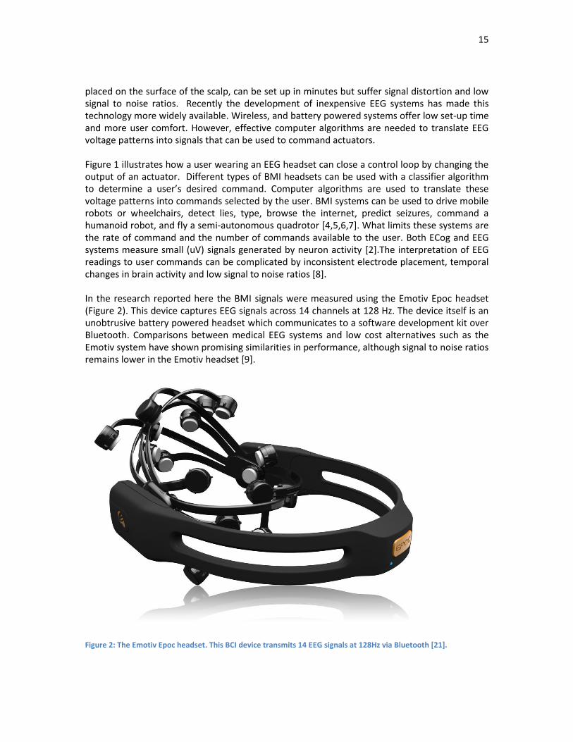
placed on the surface of the scalp, can be set up in minutes but suffer signal distortion and low signal to noise ratios. Recently the development of inexpensive EEG systems has made this technology more widely available. Wireless, and battery powered systems offer low set-up time and more user comfort. However, effective computer algorithms are needed to translate EEG voltage patterns into signals that can be used to command actuators. Figure 1 illustrates how a user wearing an EEG headset can close a control loop by changing the output of an actuator. Different types of BMI headsets can be used with a classifier algorithm to determine a user’s desired command. Computer algorithms are used to translate these voltage patterns into commands selected by the user. BMI systems can be used to drive mobile robots or wheelchairs, detect lies, type, browse the internet, predict seizures, command a humanoid robot, and fly a semi-autonomous quadrotor [4,5,6,7]. What limits these systems are the rate of command and the number of commands available to the user. Both ECog and EEG systems measure small (uV) signals generated by neuron activity [2].The interpretation of EEG readings to user commands can be complicated by inconsistent electrode placement, temporal changes in brain activity and low signal to noise ratios [8]. In the research reported here the BMI signals were measured using the Emotiv Epoc headset (Figure 2). This device captures EEG signals across 14 channels at 128 Hz. The device itself is an unobtrusive battery powered headset which communicates to a software development kit over Bluetooth. Comparisons between medical EEG systems and low cost alternatives such as the Emotiv system have shown promising similarities in performance, although signal to noise ratios remains lower in the Emotiv headset [9].

Figure 2: The Emotiv Epoc headset. This BCI device transmits 14 EEG signals at 128Hz via Bluetooth [21].

16

Two types of signals are often used with EEG BMI systems, P300 and motor-imagery signals. Motor-imagery (MI) signals are generated when users imagine specific motions such as making a fist with the left or right hand. MI signals often require weeks to months of practice to train an accurate interface and allow a user to control the amplitude of a signal on one or two axes. MI signals are known as active BMI signals as they are user controlled. MI signal training time and difficulty reduce the number of users enabled by this type of BMI system. P300 signals are generated involuntarily (passively) as a response to an external stimulus. P300 signals, or event-related potentials (ERPs), are created when a user is presented with a visual stimulus that is either recognized or desired. For example, the task of searching for a specific word in a dictionary can elicit a P300 response when the word is found. Because P300 signals are involuntary they require less training to produce a useful system. Hence, the P300 response of a user can be used as a command signal if an associated and desired visual stimulus is presented. The Emotiv Epoc headset has been demonstrated to be capable of capturing P300 visually evoked potential (VEP) and will be used in the proposed research [9]. Methods for user signal classification vary with the signal type (P300 or MI) and the portion of the data used to classify user intent. Voltage measurement at each of many electrodes can occur hundreds of times per second and such large datasets can increase the time required to detect a particular event. However in the case of P300 detection we can narrow the range of sampling to the period following a visual stimulation. Often classifiers are presented features of the raw data. For example, the maximum value observed in a certain segment of data could be a useful feature for classifying P300 events. Many different types of classifiers exist for processing features generated by a BMI and these will be discussed in Chapter 2. BMI enabled applications, such as typing, are limited by the variety and speed with which user commands can be selected [10]. For example, the ability to steer an electric wheelchair is beyond the ability of current BMI technology. This limits the freedom of BMI users to known environments or heavily automated movements. The purpose of this research is to explore and improve the techniques for identifying P300 signals in order to expand the capabilities of BMI applications.

1.1. P300 Paradigm

A P300 Event Related Potential (ERP) is characterized by a positive stimulation which reaches peak amplitude approximately 300ms following a rare stimulation event (Figure 3) [3]. The P300 signal was initially described in 1964 and 1965 when researchers noticed differences in EEG signals following visual stimuli presentation [11,2]. The original developed application of P300, the ‘P300 Speller’ allowed users to select a target letter from a 6x6 matrix of letters (Figure 4). In this application each row and column is highlighted in a randomized sequence [3]. The process of highlighting each row and column is referred to as an epoch. When a user concentrates on a single target letter, the row and column stimulation of the target letter will induce a P300 event. By comparing detected P300 events with a record of which column or row was presented, researchers were able to identify the target letter. Repeating the process of

17

highlighting each row and column increased target prediction accuracy.

Figure 3: A Sample P300 signal with a positive deflection centered near 300 ms.

Compared to other BMI interface techniques, the P300 was unique in the high number of targets which could be selected [2]. In the P300 Speller paradigm non-target letters highlighted adjacent to the target letter often create ‘noisy’ P300 stimulations, known as the ‘crowding effect’ [12]. Subject fatigue is also a limiting factor influencing target identification accuracy [1]. Electroencephalographic signals also have a low signal to noise ratio. These factors combined reduce the classification accuracy of the target and resulted in the trend of multi-epoch systems. Multi-epoch systems average results from sequential epochs to increase target classification accuracy [8]. However, multi-epoch dependency limits the overall communication rate of the system. By reducing the rate of possible commands per minute the BMI controlled application is also limited. For example, implementation of a wheelchair based P300 control system required heavy automation due to command rate limitations [4]. Because of the limitations imposed by multi-epoch systems the current research operated on a single epoch classifications.

18

A CB D E FG IH J K LM ON P Q RS UT V WXY 1Z 2 3 4

A CB D E FG IH J K LM ON P Q RS UT V WXY 1Z 2 3 4

Figure 4: An example of the classic P300 speller. Only one of the matrices above would be presented to a user. As

the rows and columns are randomly highlighted a P300 signal is elicited. With repetition the intended user selected

letter can be determined [2].

1.2. Information Transfer Rate

The metric of character selections per minute is known as the information transfer rate (ITR). Many different ITR measurement systems have been created, and no single formula best describes all BMI systems [13]. Each BMI interface system can be assessed based on the number of possible user choices, number of choices per minute and accuracy of classification [13]. One commonly used system in the BMI research field is the bit-rate measurement. However, based on the specific scenario, bit rate can be uninformative. For example, by analyzing a system with less than 50% classification accuracy a possibly high bit rate would describe a useless system where users could not make accurate selections. The bit-rate measurement system is defined in a variety of ways depending on the probability of mental states and classification error [13]. The Wolpaw bit rate, which relates classifier accuracy and number of user choices to compute bits/trial [7] is described as:

( )

19

Where P is the measured classifier accuracy of the system compared to N number of user choices. For the proposed research the Wolpaw bit-rate will be measured, and each metric will also be discussed because it is commonly used in EEG research and produced informative results in this experimental scenario.

1.3. BMI Classifiers

EEG data classification can be improved by increasing classifier accuracy and reducing the time required to select a command. Therefore we explored a number of different classifiers used in EEG research to examine which were appropriate for the Emotiv P300 combination. Machine learning classifiers use training experience to develop predictive models for classifying new data. The use of a training set and a learning algorithm results in an inference engine which addresses the classification of a new instance. An instance is often constructed of a fixed set of features that characterize the data. These features can be categorical or continuous and should be selected so that they improve the predictive accuracy of the classifier. However, feature selection can also be part of the classification problem. Large datasets containing extraneous or noisy data may provide useless or detrimental features. Therefore, the classification problem becomes twofold; first relevant features must be selected for predicting class, and second a classifier must be trained to use these features to provide acceptable classification accuracy [8]. In addition to classification accuracy of training data the inference engine must classify new data to an acceptable degree. This results in a tradeoff where classifiers often suffer from ‘over-fitting’ resulting in high accuracy classifying training data and low accuracy classifying new data. Many classifier systems have been implemented to detect P300 signals following a known positive stimulation. Linear discriminant analysis (LDA), support vector machines (SVM), stepwise linear discriminant analysis (SLDA), Fisher’s linear discriminant (FLD), Bayesian linear discriminant analysis (BLDA), Pearson’s correlation method and many other methods produce linear and non-linear solutions for P300 detection [8]. P300 detection becomes a binary classification problem where datasets containing possible P300 are classified as positive stimulation events or non-events. Classifier accuracy can also be determined in a number of ways including total event and non-event classification success, or only positive stimulation detection accuracy, depending on the BMI application. To assess overall classifier accuracy both event and non-event accuracy are considered [14]. Discriminant functions, such as LDA classifiers are a common choice in published P300 research and are capable of achieving 95% or greater classification accuracy when multiple P300 signals are averaged [8]. These discriminant functions attempt to create a prediction of class based on the linear combination of known observations. An example of a two dimensional LDA function is shown in Figure 5.Linear discriminant analysis seeks to reduce dimensionality of feature data while preserving discriminatory information. By maximizing a linear function to separate two classes LDA methods develop discriminatory functions for classifying data. Fisher’s linear discriminant solution uses the within class scatter to improve the linear discriminant function. Compared to other classification methods, LDA offer easy to interpret between feature differences and fast training and classification times. However, complex classification problems have shown that LDA can often be outperformed, in terms of classification accuracy, by non-

20

linear classifiers [15].

Figure 5: Linear Discriminant Analysis binary classification [16].

Another classifier option is using an artificial neural network (NN). Neural networks offer a non-linear approach, and are theoretically based on biological neural networks. In a given NN a subset of ‘neurons’ act to classify input arguments to an output class (Figure 6). Neural networks approximate non-linear relationships by tuning the weights of these neurons using classified data [15]. Because these systems use predefined examples of classified data they are referred to as supervised learning algorithms. NNs have been successful in classifying noisy hard to solve problems such as speech recognition and computer vision and therefore have also been applied to EEG data classification. Neural networks have been used successfully in P300-detection [17]. Neural networks offer a robust method for classifying P300 features because they implicitly detect complex interactions between predictor features. Unfortunately, the classification function generated by a NN does not give insightful information explaining the relationship between input features and output classification. Each neuron is connected to each input creating an irreducible cross network between inputs and output. The magnitude of the weights relating an input and output cannot be used to interpret the importance of a single feature on predicting an output. Furthermore, NNs are prone to over-fitting as feature and neuron interconnections increase [15]. Support Vector Machines (SVM) are another classification technique explored in this thesis. By

21

comparing the points closest to the class boundary SVM create support vectors to define a new class boundary. SVMs can increase dimensionality of datasets, making it more likely that the problem becomes linearly separable. The SVM classifier has been used on P300 data with success, SVM offers fast classification with low preprocessing requirement [18].

Feature 1 Feature 2 Feature 3

Neuron Neuron Neuron

Output output

Input Layer

Hidden Layer

Output Layer

Figure 6: Sample artificial neural network showing interconnectedness between inputs (features) layer, hidden

layer containing neurons connected to each input, and output layers which provide class estimation. Each

connection contains a weight value and each neuron contains a bias value. These values are adjusted using the

back-propagation training method to tune the NN classifier.

Support vector machines are classified as supervised, non-probabilistic, binary linear machine learning algorithms [19]. Support vector machine classifiers construct sets of hyperplanes to maximize discriminant margins between training classes, as seen in Figure 7. Support vector machines have shown success in classifying P300 signal data [8]. Similarly to neural networks the resultant discriminant functions generated from a trained SVM classifier are difficult to interpret as distance from a class defining hyperplane is not related to class probability.

22

Figure 7: Support Vector Machine binary classification showing three support vectors, the decision boundary and

the decision margin [16].

BMI classifiers can be compared by assessing how often the intent of the user matches the classifier output (Figure 8). Most classifiers use specific features of the data to determine a class, rather than the entire dataset. This improves classification time by reducing the dimensions of input data. Similarly, depending on the sampling rate of the BMI, some EEG systems are also down-sampled for sample reduction. Some examples of the features that are extracted from raw signal data and that have been used to classify P300 signals include signal amplitude, maximum values, minimum values, and wavelet cross correlation values [20]. Furthermore, channel selection criteria may reduce the number of electrodes included in feature extraction to reduce sample size and exclude unnecessary electrode data.

1.4. Feature Selection Rather than providing classifiers with large amounts of raw data, features are selected to describe these data and optimize classifier performance. Features can be subsections of raw data, or values extracted from raw data, such as the slope of a segment. Various feature extraction techniques can be used to reduce raw data to informative and classifiable features. In the field of P300 detection, principal and independent component analyses have been used to produce subject specific features [21]. Alternatively, genetic algorithms can be used to examine a wide variety of features and attempt to find feature combinations for successful data classification.

23

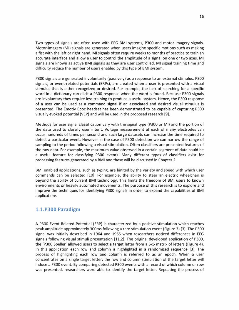
Figure 8: A comparison of classification accuracy using Fisher’s Linear Discriminant Analysis (LDA), Bayesian linear

discriminant analysis (BLDA), stepwise linear discriminant analysis (SWLDA), a feature extraction linear classifier

method (FE), linear support vector machine (SVM), multilayer perceptron (NN), and a Gaussian kernel support

vector machine (nSVM). The analysis shows the classification accuracy with increasing numbers of averaged

stimulation events, or epochs, in the P300 speller [8].

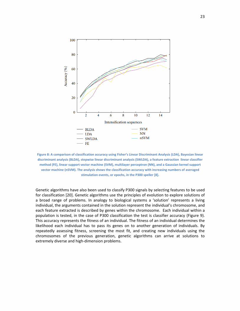
Genetic algorithms have also been used to classify P300 signals by selecting features to be used for classification [20]. Genetic algorithms use the principles of evolution to explore solutions of a broad range of problems. In analogy to biological systems a ‘solution’ represents a living individual, the arguments contained in the solution represent the individual’s chromosome, and each feature extracted is described by genes within the chromosome. Each individual within a population is tested, in the case of P300 classification the test is classifier accuracy (Figure 9). This accuracy represents the fitness of an individual. The fitness of an individual determines the likelihood each individual has to pass its genes on to another generation of individuals. By repeatedly assessing fitness, screening the most fit, and creating new individuals using the chromosomes of the previous generation, genetic algorithms can arrive at solutions to extremely diverse and high-dimension problems.

24

Evolution Genetic Algorithm

Fitness Determined

More Fit Less Fit

Fitter Individuals Reproduce

More

Immigration and Mutation Introduce

Randomness

Random Solutions To a Problem

Each Solution is Tested

More Fit Less Fit

Fitter Solutions Contribute More To A New Group Of

Solutions

Some Randomness Is Added To New Set Of Solutions

Figure 9: Comparison of a genetic algorithm to the principles of biological evolution. In a genetic algorithm a

solution to a problem behaves as an individual would in a biological system. Each solution must compete with

other solutions in order to determine its fitness. The most-fit individuals do not move to the next generation but

are combined with other members of the population to produce a new generation of individuals. This process is

repeated until a certain number of generations have passed or a targeted fitness is achieved. Randomness included

in the process prevents fixation of the population and increases solution space exploration.

1.5. Multi Epoch Averaging

Because P300 signals have a low signal to noise ratio methods have been developed to increase classification by using repeated samples to classify a user’s selection [1]. Each visually evoked stimulus can be referred to as an epoch. By averaging raw data or features between epochs P300 signals become more distinct and classifier accuracy improves, as is seen in Figure 8 where ‘Intensification sequences’ are averaged epochs. This is a useful technique where high accuracy is required but also results in reduced possible commands per minute. Depending on the application of the BMI it may be desirable to increase commands per minute by reducing the number of required epochs. Therefore, in this thesis we explore methods of reducing epoch averaging while retaining classifier accuracy and usability of the system. We attempt to use a single epoch for steering command selection of a mobile robot, and explore reduced epoch averaging systems.

25

1.6. Research Objective Existing BMI technologies have demonstrated a unique method of enabling victims of locked in syndrome. P300 signal classifiers offer both high accuracy and a potentially high numbers of user command choices and are therefore ideal for BMI applications. However, because repeated epochs are required to determine a user selection the number of possible choices per minute, or command rate, is low. Command rate constrains the type of application which a BMI system can control. For instance, wheel-chair control is limited to destination selection, while the actual movement of the chair is highly automated. This limits the application use to previously mapped environments and similarly limits the freedom of the user. To allow a user to navigate an unknown environment the user must be able to select commands much more quickly. To increase the application range of BMI control systems this research aims to improve command rate by exploring single-trial P300 classification. Single-epoch systems potentially offer the highest rate of commands, but have reduced classification accuracy. Therefore, we explored feature selection to improve single-epoch P300 classification. Specifically, we explore the use of a genetic algorithm to select features which best describe a P300 event. We use this information to improve P300 classification and also test a number of P300 classifiers for single-epoch detection. We identify features most useful in categorizing single-epoch P300 events between subjects to find trends in the population. We believe that these contributions will be beneficial for improving future P300 applications.

26

CHAPTER 2 SINGLE-TRIAL P300 DETECTION USING A GENETIC ALGORITHM FOR FEATURE SELECTION AND A LOW-COST EEG

HEADSET

2.1. Introduction

Current P300 BMI systems are limited maximum user command rate. Single-trial classification techniques provide the highest potential command rate but classifying these signals is extremely challenging due to low SNR. One option for improving single trial signal classification is to use a genetic algorithm (GA) to find sections of data which better represent user intent. Genetic algorithms use populations of solutions which ‘evolve’ over time to solve complex non-linear problems [20]. They offer a method for thorough exploration of a solution space and sometimes avoid local minima that can trap linear techniques. Using a genetic algorithm may produce accurate signal features for fast P300 detection. Here we describe the technique and results of a single-epoch P300 detection experiment where features are selected by a genetic algorithm. This GA was used to train both neural networks and LDA classifiers to detect P300 events. We also compare the features selected by the GA between subjects. Finally we compare NN and LDA classifiers and their ability to classify new data. This chapter is divided as follows. Section 2.2 discusses the system architecture and modules involved in the P300 signal identification. Section 2.3 presents the experimental results found with three subjects. Finally, Section 2.4 concludes the chapter and suggests future work.

2.2. Methods

In this section the system architecture, the hardware, the classification algorithms and the genetic programming approach are explained. Finally, the data collection using three subjects is discussed.

2.2.1. System Architecture

The first problem an EEG classification system needs to address is the synchronization of the visual display and EEG response. Therefore, a data collection module was developed in order to synchronize the appearance of the visual stimuli and the recordings of the EEG signal. The data collection system (2.2.2) included EEG referencing and filtering, such that the DC bias for all signals was removed. Following data collection, the entire dataset was passed to the genetic algorithm (2.2.4), which selected features for both a NN and LDA classifier (2.2.3).

27

The whole system is depicted in Figure 10with the interfaces between all the modules. The visual display module was developed in Blender on a Linux Operating System (OS), while the data collection module, using the provided Emotiv drivers, was implemented in C++ on the same machine. Both the GA and NN were implemented in MATLAB. The result is a set of features that improve the classification of events derived from the filtered data presented during training.

BMI Headset

Genetic

Algorithm

Data

Collection

Visual Display

Feature Selection,

Trained NN

Figure 10: Overview of the novel BMI system created for data collection, genetic algorithm and classifier training.

Colours indicate development language (Blue: Blender, Green: C++, Orange: Matlab).

2.2.2. Data Acquisition

BMI signals were measured using the Emotiv Epoc headset (Figure 2). This device captures EEG signals across 14 channels at 128 Hz (Figure 11). International 10-20 locations: AF3, F3, F7, FC5, T7, P7, O1, O2, P8, T8, FC6, F4, F8, AF4, and references Common Mode Signal (CMS) and Driven Right Leg (DRL). The references CMS/DRL are used to normalize the channel data and remove some externally generated noise. The device itself is an unobtrusive battery powered headset which communicates to a software development kit over Bluetooth. Comparisons between medical EEG systems and low cost alternatives such as the Emotiv system have shown promising similarities in performance, although SNRs remain lower in the Emotiv headset [9], which makes the classification of the signals more challenging. The headset has been demonstrated to be capable of capturing P300-Visually Evoked Potential (VEP) [9]. Data recorded by the headset is referenced against electrodes CMS and DRL. The referenced data is then band pass filtered with a 4th order Butterworth filter (0.1 -60 Hz) in order to remove unwanted frequency effects and biases, a common P300 filtering technique [22].

28

Figure 11: EEG electrode placement locations for the Emotiv Epoc; those with a solid black circle indicate the

electrodes used in this study forP300 classification.

2.2.3. Classifiers

A normal P300 signal usually lasts for around 500ms (Figure 16). For our system, following a stimulation event, 100 samples representing 780ms post-stimulation were used for feature extraction to ensure the signal was fully captured. The features selected will be discussed in Section 2.2.4.

Following feature extraction, a back-propagation neural network classifier was trained and tested. The testing dataset was not used during training of the network. Each dataset originally contained three non-target signals for each target signal due to the four choice design. To reduce classifier biasing non-target signals were randomly down-sampled so that the ratio of target and non-target signals was equal. The NN received 10 inputs (features), and produced 100 input weights, 10 hidden neurons, 10 bias weights, and a two layer output with a sigmoid activation function. For training of the classifiers, non-stimulation events were randomly selected so that the ratio of stimulation and non-stimulation data was equal. In this thesis, three different classifiers are used, the artificial neural network, a non-linear predictive model, a linear discriminant analysis classifier, and the SVM. These classifiers were used because they are

29

common methods in the related literature and represent both linear and non-linear techniques [17,9]. Classification accuracy was calculated as the number of correctly identified stimulation and non-stimulation events compared to the total number of events.

2.2.4. Genetic Algorithm

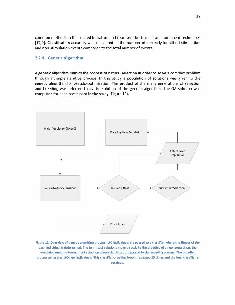
A genetic algorithm mimics the process of natural selection in order to solve a complex problem through a simple iterative process. In this study a population of solutions was given to the genetic algorithm for pseudo-optimization. The product of the many generations of selection and breeding was referred to as the solution of the genetic algorithm. The GA solution was computed for each participant in the study (Figure 12).

Initial Population (N=100)

Neural Network Classifier

Fittest From Population

Breeding New Population

Best Classifier

Take Ten Fittest Tournament Selection

Figure 12: Overview of genetic algorithm process. 100 individuals are passed to a classifier where the fitness of the

each individual is determined. The ten fittest solutions move directly to the breeding of a new population, the

remaining undergo tournament selection where the fittest are passed to the breeding process. The breeding

process generates 100 new individuals. This classifier-breeding loop is repeated 15 times and the best classifier is

retained.

30

An example of a GA solution is a set of 10 combinations of which each describe a feature selected using the arguments: EEG channel, segment of data, and mathematical operation performed on these data Figure 13.

Channel: O1Feature:

MaximumSegment: 0-780ms

sChannel: O1 Segment: 0-780ms Feature: Maximum

x10

Figure 13: An example solution generated by the genetic algorithm showing one of 10 genes. Each gene is

composed of three arguments, channel selection, segment selection and feature operation. In this example the

first gene describes extraction of the maximum value from the O1 channel in the 0-780ms post stimulation. Each

solution contains 10 of these genes.

To start the algorithm a randomly selected population of 100 individuals was generated. Various population sizes were examined and 100 individuals was observed to be adequate to maintain diversity through 15 generations. An ‘individual’ represents one possible solution in a population of individuals. Each individual contained a chromosome with 10 genes. This number of genes was not tested but was selected based on similar genetic algorithm studies [20]. Each gene contained three arguments that were instructions for feature extraction (2.2.5).

The genetic algorithm produced and selected genes to extract features from raw data for the classifier. Each individual was passed to a NN classifier where the encoded features were extracted from raw data. These features were used to train and test the classifier. Following classification the re-substitution error of the verification data was used to represent the fitness of the individual. The fittest 10 individuals were passed directly into the gene pool of the next generation, a process known as elitism (Figure 14). The remaining individuals competed in tournament selection where four randomly selected individuals were compared and the fittest individual was passed into the gene pool. Five new individuals were randomly generated and added to the new gene pool to represent mutation and immigration.

Following selection a new population was created using those individuals selected for the gene pool. New individuals were created through the combination of two randomly selected individuals from the gene pool. From each of these parents sections from each chromosome were randomly combined. The chromosomes were combined by selecting segments (4) from

31

each parent to be passed on to the offspring. The new population of 100 offspring began the fitness-selection process again. The genetic algorithm operated for 15 generations, which was observed to be sufficient at representing the plateau of results the algorithm produced (Figure 18).

Tournament Selection With Elitism

Fitness Determined

More Fit Less Fit

ElitismTournament

Selection

Breeding Population

Figure 14: The selection process used for the genetic algorithm. Elitism is the process where the fittest individuals

are passed directly into the breeding population. Tournament selection is completed on the remaining individuals.

In tournament selection groups of individuals are selected randomly from the population and the fittest of the

group is passed to the breeding population.

32

2.2.5. Feature Extraction Each gene was composed of three numbers ranging from 1-14. Each gene contained information for; channel selection; mathematical operation; and data segment.

Channel Based on preliminary observations EEG channels T7, T8, P7, P8 and O1, O2 were included in possible channel selection (Figure 11). These channel selections coincided with other research observations that P300 is most discernable in the parietal region of the brain [20,19]. Eight other channel options compared differences between certain channels and averages of channel. We compared channels to improve noise reduction and isolate regional EEG activity. We examined the average of the left hemispherical electrodes T7/P7/O1, the average of right hemispherical electrodes P8-T8-O2, and the difference between the left and right electrodes (T8/P8/O2 - T7/P7/O1).We also compared each electrode pair (T7 – T8; P7 – P8, and O1 –O2). To examine differences between anterior and posterior electrode we compared the average of O1/O2 to the average of T7/T8. Finally all the channels were averaged for an overall signal measure.

Temporal Segment The temporal segment gene determined the portion of the 100 samples to use for feature extraction. Figure 16shows a sample EEG signal with the fourteen data segments ranging from 10-75 samples in length and covering the full 100 sample set. The range of the segments included were : 0-50, 50-100, 25-75, 25-50, 50-75, 0-75, 25-100, 30-40, 40-50, 50-60, 20-30, 60-70, 10-20, 70-80. As we sampled the electrodes at 100 Hz these segments could also be represented as ms ranges: 0-391 ms, 391-781 ms, 195-586 ms, 195-391 ms, 391-586 ms, 0-586 ms, 195-781 ms, 78-156 ms, 156-234 ms, 234-313 ms, 313-391 ms, 391-469 ms, 469-547 ms and 547 – 625 ms.

Mathematic Operation Seven mathematical operations reduced the channel and segment data to a single value feature. The operations included; maximum value, minimum value, the highest power coefficient of a second degree fitted polynomial, slope, and cross correlation with one of three weight functions. The three weight functions are shown (Figure 15). These weight functions are similar to functions which have previously been demonstrated as viable targets for classifiers and mimic the positive deflection observed in a P300 signal [20].

33

Figure 15: Weight functions used for cross-correlation feature extraction.

Figure 16: A sample P300 signal (red-continuous) shown with a positive peak at 250-300ms. The temporal feature

segments (blue-horizontal segments) are also shown.

34

2.2.6. Subject Data Collection

Three participants volunteered for this study. Each participant was tested individually. All participants were all able to complete the experiment in one sitting, which lasted less than 30 minutes. The subject was comfortably seated 30 cms from a laptop and presented with a simple visual display where four letters (A, B, C and D) were shown in each corner of the display. These letters are referred to as the targets. A bright green box was presented behind the target on the screen (Figure 17). This was the method of highlighting a target to elicit stimulation.

After fitting and adjusting the headset the subject was asked to count the number of times one of the four targets was highlighted. The targets were highlighted in a random sequence. The probability of occurrence of a given target being highlighted is 25%. Targets were highlighted for 333ms followed by 333ms without any highlighting, therefore inter-stimulus period was 666ms for any two stimuli and 2.7 seconds for target stimuli. The instructed target letter was switched after a random number (20-30) of samples so that each letter was counted. This was repeated twice. The first dataset was used for training a NN and LDA classifier using the genetic algorithm as described above. The second verification dataset was used to test the NN and generate the fitness of the NN.

2.3. Results

2.3.1. Genetic Algorithm Results

The results of the genetic algorithm (referred to as solutions) were compared to examine which channels, features and segments contributed most to detecting the P300 event. We compared the occurrence of specific gene arguments within individual solutions and across the population of solutions. The solution to a genetic algorithm was the fittest individual measured over fifteen generations (Figure 18).

When comparing the results of channel selection, we found those channels which were calculated as the difference of sets of other channels most influential on predicting P300 events. In particular, the difference between the anterior electrodes (T7/T8) and posterior (O1/O2) electrodes was observed four times in the solution sets. The combination of all electrodes was observed often (n=4) and the O1/O2 electrodes were the most common electrode set in the solutions. The O1/O2 set has been found to be influential in other P300 studies [14]and matches our observations that the parietal region of the brain was highly correlated with P300 events.

35

Figure 17: Visual display with possible targets A, B, C & D and ‘C’ highlighted as the target. Each target was

randomly highlighted for 333ms followed by 333ms where none of the targets were highlighted. Although the

ordering of the targets being highlighted was random all four were highlighted before a new sequence began.

Table 1: Instances of repeated gene combinations (Operation-Op, Channel-Ch Segment-Seg) found within two

solutions generated by the GA.

Seven mathematical operations were also included as genes. The most common operation gene in the populations of solutions was the cross correlation value generated by the W1 function (n=7 of total = 30). The W1 cross correlation was the only operation observed in multiples in all solutions. The polynomial coefficient calculation was also common in solutions (n=6).

Gene Groups

Repeated Gene Combinations

Gene 1 Gene 2 Subject Subject 2

Op/Ch Wave1 P7 S1 S2

Op/Ch Wave1 T7/P7/O1 –T8/P8/O2

S1 S3

Op/Ch Max All Channels Average

S1 S3

Op/Ch Slope O1-O2 S2 S3

Op/Seg Wave1 390-585ms S1 S3

Op/Seg Polynomial

390-780ms S1 S2

Op/Seg Wave3 390-468ms S1 S2

36

Fourteen data segments were compared which ranged from 0 to 100 samples post stimulation (780ms). The most common segment found in the solutions generated by the GA was the 195-390ms samples segment (n=7). This result corresponds well with P300 research which focuses on the 300ms area of samples. Of the temporal sections which only included 10 data samples the most common was the 312-390ms segment that captured the decline of the positive deflection following a P300 event (n=4).

Figure 18: Progress of the genetic algorithm showing individuals (small multi-coloured horizontal bars), generations

of individuals (x –axis) and P300 classification accuracy (y-axis). The various colors of each individual represent the

feature extraction arguments it contains. The population begins with randomly selected combinations as seen at

generation one. As the number of generations increase the population becomes more similar and a classification

accuracy plateau is achieved. This can be seen by the vertical bands of colors showing common gene arguments in

the population past 12 generations.

Instances of combinations of genes found between solutions were rare and in no cases were the same gene combinations found in all three solutions. The fitted polynomial coefficient of channel O2 was found in the solutions from Subject 1 and 2 (Table 1). The slope of the combination of all the electrode channels was found in Subject 2 and 3. Recurring gene combinations of operations and data-segment were found four times. Segments 195-780ms and 190-390ms were found in combination with the W1 cross correlation and the fitted polynomial

37

coefficient operation respectively in both subjects 1 and 2. The number of GA solutions representing the data segments following 190ms was not surprising. As the name implies the P300 stimulation is observed in this data as a large positive deflection which begins near 200ms, dips below 0 near 420ms and is complete by 700ms (Figure 16). This area was highly influential on the solutions generated by this study.

2.3.2. Classifier Accuracy

Following training the NN classifier used to predict the fitness of an individual was tested on a preserved segment of the data it was trained on, and also on two entirely unknown datasets. A LDA classifier was also trained with the same features as the NN and the re-substitution error was included for comparison (Table 2). On average the neural network classifier reached single-epoch P300 detection accuracies of 76.4%. The most accurate P300 systems developed have used independent component analysis and variation analysis to achieve 80% or higher single-epoch detection with the classic P300 paradigm system with 36 selection options [21]. However this system required researchers to examine and select independent components for each subject, and used a medical grade EEG headset. The system presented in this research requires no guidance to train a classifier. In a scenario where a single stimulus is presented and the subject watched for a specific signal Li et al, constructed a neural network classifier which achieved 65% single-epoch accuracy [18]. Compared to both these systems this research was completed with a lower fidelity BMI device and was successful in detecting single P300 events with similar accuracy. Verification datasets show that classifiers do not maintain the same level of predictive accuracy on new datasets. The verification classifier accuracy for subject 1 and 3 varied significantly (p<0.05) from the original NN classification accuracy. The LDA results were similar to those generated by the trained NN demonstrating that the selected features were predictive regardless of the classifier.

Table 2: Classification accuracy results of the GA trained NN classifier and LDA classifier. The NN classifier was

tested on a novel dataset for verification (Ver). The Wolpaw bit rate of the verification accuracy is also presented.

NN LDA Ver Bit Rate

S1 73.7 72.1 70.2 14.4

S2 79.5 74.3 66.0 11.9

S3 75.9 73.3 65.3 11.5

Average ± SD 76.4±2.9 73.3±2.9 67.4±2.6 12.6±1.57

38

2.4. Conclusion

In conclusion we found the GA to be a successful technique for training NN and LDA classifiers. The GA was also successful in identifying features which were associated with P300 events. We observed that features from data 190ms post stimulation were associated with higher prediction accuracies. Results from cross subject data will require more participants to increase statistical power. This data could be used to improve P300 predictions on users without training and would improve user satisfaction. Further comparisons will also allow us to identify features found in a broader population. Furthermore by increasing single-epoch P300 detection speed and accuracy we intend to enable novel experimentation with P300 signals, especially with the remote operation of mobile robots.

39

CHAPTER 3 EXTENDED POPULATION STUDY

3.1. Introduction

Brain machine interface systems allow users to select computer commands using signals generated from thought. The BMI systems ability to accurately interpret the user’s intent is fundamental for successful BMI as it increases efficiency and user satisfaction. To increase BMI classification we explored the use of a GA to select features for a linear (LDA) and non-linear (NN) classifier as described in Chapter 2. Our preliminary research in P300 detection found that some of the posterior electrodes (O1, O2, P7, P8, T7, and T8) were highly influential on signal classification accuracy. We also found that the segment of data starting 190ms post stimulation event was more useful in predicting P300 event. These results suggested our GA system produced viable features for P300 detection, as the post 190ms time segment results fits with other P300 studies. However, as the first experiment only included three subjects we suggest that by including more participants in the P300 feature extraction process we may be able to determine more trends in P300 detection.

In addition to the increased participant number we tested a further classifier, the support vector machine (SVM). A number of P300 experiments have demonstrated high accuracy P300 classification using SVM techniques [8]. Furthermore, compared to neural networks SVMs represent convex optimization problems and therefore guarantee unique global optima. Back propagation neural networks, such as those used in Chapter 2, can converge to local rather than global minima [23]. Therefore we include the SVM in our analysis as a possible method of improving P300 classification accuracy.

3.2. Methods

Following exactly the same process as the data collected in Chapter 2 the study was expanded to include 10 more individuals ranging in gender and age (13-55). Each subject was asked to count the number of times one of four possible targets was visually highlighted. The target letter was changed throughout the experiment so that each letter option was counted. The experiment included 100 stimulation events divided between the four options. The experiment was repeated three times per individual and subjects were asked not to remove the headset or reposition it during the experiment. Following data collection the entire dataset for all individuals was passed to the genetic algorithm to find classification predictor feature for each individual. Data collected in Chapter 2 was included in results analysis to improve statistical resolution.

We used the Matlab R2012a SVM function with a linear kernel function to train and classify the data. A linear kernel was used because it increased the speed of both the classification process and implementation for live testing.

40

3.3. Results

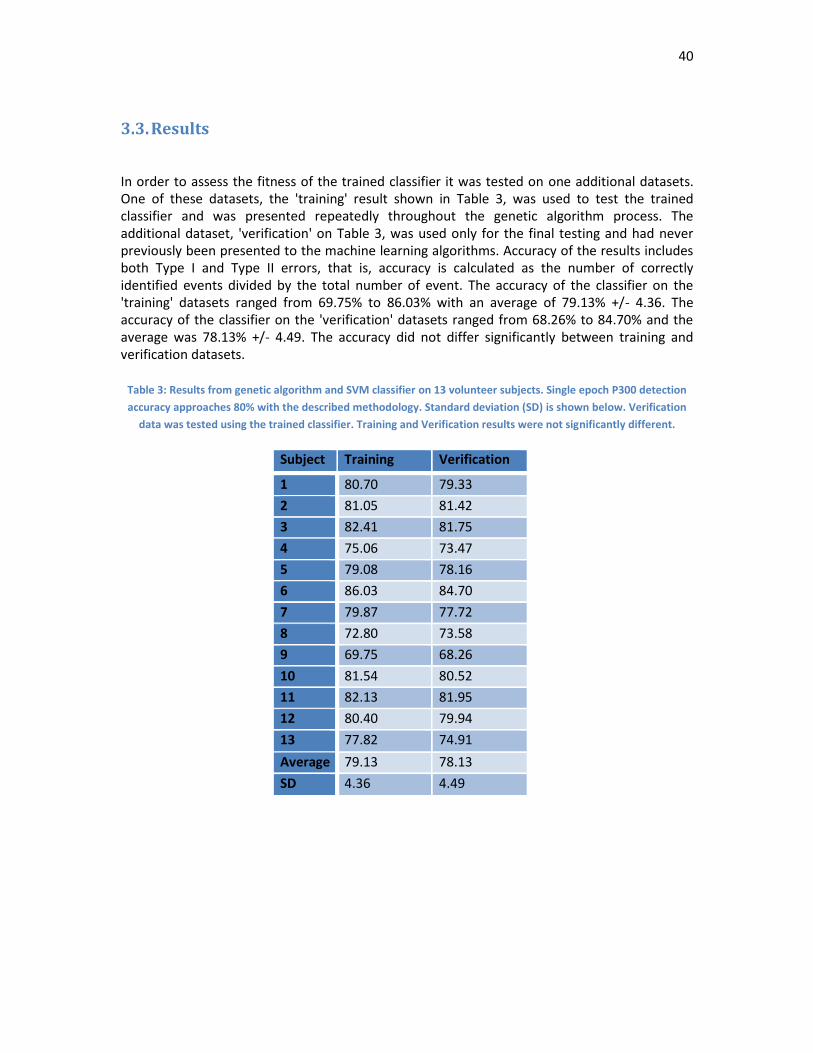
In order to assess the fitness of the trained classifier it was tested on one additional datasets. One of these datasets, the 'training' result shown in Table 3, was used to test the trained classifier and was presented repeatedly throughout the genetic algorithm process. The additional dataset, 'verification' on Table 3, was used only for the final testing and had never previously been presented to the machine learning algorithms. Accuracy of the results includes both Type I and Type II errors, that is, accuracy is calculated as the number of correctly identified events divided by the total number of event. The accuracy of the classifier on the 'training' datasets ranged from 69.75% to 86.03% with an average of 79.13% +/- 4.36. The accuracy of the classifier on the 'verification' datasets ranged from 68.26% to 84.70% and the average was 78.13% +/- 4.49. The accuracy did not differ significantly between training and verification datasets.

Table 3: Results from genetic algorithm and SVM classifier on 13 volunteer subjects. Single epoch P300 detection

accuracy approaches 80% with the described methodology. Standard deviation (SD) is shown below. Verification

data was tested using the trained classifier. Training and Verification results were not significantly different.

Subject Training Verification

1 80.70 79.33

2 81.05 81.42

3 82.41 81.75

4 75.06 73.47

5 79.08 78.16

6 86.03 84.70

7 79.87 77.72

8 72.80 73.58

9 69.75 68.26

10 81.54 80.52

11 82.13 81.95

12 80.40 79.94

13 77.82 74.91

Average 79.13 78.13

SD 4.36 4.49

41

3.3.1. Count Data

The results given by the genetic algorithm, referred to as a solution, was a 10 gene chromosome (Figure 13). Each gene contains three arguments, an EEG channel selection, a segment of data post stimulation, and a mathematical operation performed on this data segment. The first comparison made was a simple count of the occurrence of each argument in the population of solutions. For the EEG channel and post-stimulation data segment 14 options were possible, while the mathematical operation had seven options. With 13 individuals and 10 genes, 130 arguments were included in the full population. If these arguments were randomly distributed throughout the gene options we would predict 9.3 counts per argument for channel and segment, and 18.6 counts per mathematical operation.

Channel Count Channel data was a combination of raw channels (T7, P7, O1, T8, P8 and O2) and channel comparisons. Left – right represents the channels on the left side of the brain (T7, P7, O1) subtracted from those on the right (T8, P8, O2). Each electrode pair was also compared (T7-T8, P7-P8, and O1-O2). The electrodes placed further towards the front of the head were compared to those near the back (T7/T8 – O1/O2). All channels were also grouped and averaged into one.

Channel count data was not significantly different from a random distribution (p>0.05) when count data was compared using the chi-squared goodness of fit test (Figure 19). Counts ranged from 3 to 23 occurrences (T8 and Back – Front). The channel which represented the difference between the back electrodes to the front electrodes was most common in the solutions (n = 23, p = 0.058). The channels representing the front of the electrodes measured were the least common in the solutions (T7 n = 4, T8 n = 3).

42

Figure 19: Occurrences of channel selection arguments in the population of solutions found with the genetic

algorithm (n = 130).

Mathematical Operation Count As described in the methods section of Chapter 2 the mathematical operations (7) performed on the data segments included the following: maximum value, minimum value, coefficient of polynomial, cross correlation with one of three waveforms, and the slope of the segment. When combined with channel and segment arguments the mathematical operation resulted in a single value which was used as a feature for the classifier. The genetic algorithm produced 13 solutions which each contained 10 mathematical operation arguments (Figure 20).

Operation count data was not statistically different than a random distribution of counts when compared using a chi-square goodness of fit analysis (p>0.05). The range of observed counts was 15-28 observations (Max/Min and Cross correlation with wave 1). Wave 1 cross correlation was the mathematical operation found most often in the population of solutions (n = 28, p>0.053). The remaining six operations each had counts ranging from 15-19 observations, similar to the null-hypothesis expected count of 18.57.

Channel

0

5

10

15

20

25

Co

un

t

Channel Count in GA Solutions

43

Figure 20: Number of observations of seven mathematical operations found in the solution population

produced by the genetic algorithm. (N = 130)

Segment Count Following a visual stimulation event 100 samples were recorded on all channels to capture the expected P300 deflection. At a sampling rate of 128 Hz the electrodes data following a VEP covered 781 ms. The segment argument used for selecting subsections of this data included the following: 0-391 ms, 391-781 ms, 195-586 ms, 195-391 ms, 391-586 ms, 0-586 ms, 195-781 ms, 78-156 ms, 156-234 ms, 234-313 ms, 313-391 ms, 391-469 ms, 469-547 ms and 547 – 625 ms. These segments divided the 100 samples in a number of ways (586 ms segments, 391 ms segments, 195 ms segments and 78 ms segments.

The distribution of occurrences of segment arguments in the population of solutions found using the genetic algorithm did not differ significantly from a random population distribution (p>0.05). The range of counts varied from 2-26 observations (segment 156-234 ms, 195-391 ms). The most commonly found segment argument was the 195-391 ms section (N = 26, p= 0.054). The 78 ms segments dividing the 0-625 ms post stimulation were on average less common in the solution set (expected: 65, observed: 44) while all other segment lengths were more common than expected.

Mathematical Operation

0

5

10

15

20

25

30

Max Min PolyCo W1 W2 W3 Slope

Co

un

t

Mathematical Operation Count in GA Solution

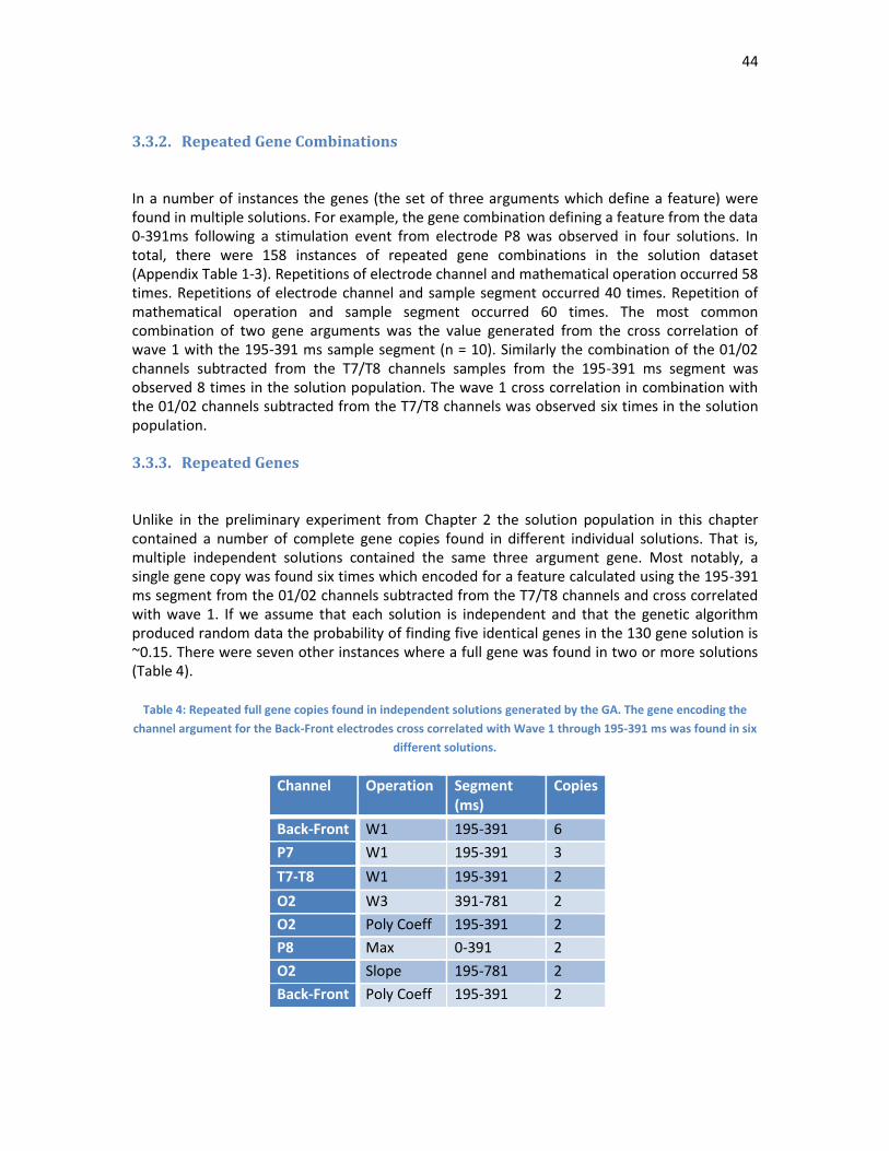
44

3.3.2. Repeated Gene Combinations

In a number of instances the genes (the set of three arguments which define a feature) were found in multiple solutions. For example, the gene combination defining a feature from the data 0-391ms following a stimulation event from electrode P8 was observed in four solutions. In total, there were 158 instances of repeated gene combinations in the solution dataset (Appendix Table 1-3). Repetitions of electrode channel and mathematical operation occurred 58 times. Repetitions of electrode channel and sample segment occurred 40 times. Repetition of mathematical operation and sample segment occurred 60 times. The most common combination of two gene arguments was the value generated from the cross correlation of wave 1 with the 195-391 ms sample segment (n = 10). Similarly the combination of the 01/02 channels subtracted from the T7/T8 channels samples from the 195-391 ms segment was observed 8 times in the solution population. The wave 1 cross correlation in combination with the 01/02 channels subtracted from the T7/T8 channels was observed six times in the solution population.

3.3.3. Repeated Genes

Unlike in the preliminary experiment from Chapter 2 the solution population in this chapter contained a number of complete gene copies found in different individual solutions. That is, multiple independent solutions contained the same three argument gene. Most notably, a single gene copy was found six times which encoded for a feature calculated using the 195-391 ms segment from the 01/02 channels subtracted from the T7/T8 channels and cross correlated with wave 1. If we assume that each solution is independent and that the genetic algorithm produced random data the probability of finding five identical genes in the 130 gene solution is ~0.15. There were seven other instances where a full gene was found in two or more solutions (Table 4).

Table 4: Repeated full gene copies found in independent solutions generated by the GA. The gene encoding the

channel argument for the Back-Front electrodes cross correlated with Wave 1 through 195-391 ms was found in six

different solutions.

Channel Operation Segment (ms)

Copies

Back-Front W1 195-391 6

P7 W1 195-391 3

T7-T8 W1 195-391 2

O2 W3 391-781 2

O2 Poly Coeff 195-391 2

P8 Max 0-391 2

O2 Slope 195-781 2

Back-Front Poly Coeff 195-391 2

45

3.3.4. Probability of repeated genes

With a population of 13 solutions each containing 10 genes the total number of genes analyzed was 130. The genetic algorithm attempted to select individuals who possess the best genes for extracting P300 indicative features. However, to assess the results of the genetic algorithm we will compare findings to the null hypothesis, that the genes selected by the GA were entirely random. Therefore, through experimentation, we have created a table of probabilities to assess the random-likelihood of finding repeated gene combinations (Table 5).

Table 5: Experimentally derived probability of finding n repeated combinations of gene arguments in the 130

sample population solution. Probability of combinations of channel and segment (14x14), channel or segment and

mathematical operation (14x7) and full gene (14x14x7) are shown. Probability was calculated through simulation

of 1000 trials.

Combination

Repeats 14x7 14x14 14x14x7

4 1 1 0.1

5 1 0.63 0.032

6 0.704 0.11 0.0002

7 0.22 0.011 <0.0001

8 0.035 0.002

9 0.008 <0.001

10 0.0007

3.4. Discussion

Two main results were generated from this chapter. The genetic algorithm produced a single set of features for each included subject which was found most useful in predicting P300 event. Next the genetic algorithm and classifier produced a test and verification accuracy which we will use to discuss the classifier validity and the applicability of single-epoch P300 systems.

3.4.1. Gene Count Data

Each feature was encoded by a set of three genes. As each individual solution contained 10 features and because 13 subjects were included we were able to combine and analyze 390 genes or 130 genes for each feature argument. Those arguments were; channel, segment and operation and each of these arguments had a range of choices (channel: 14, segment: 14, operation: 7). When we examined the final set of 130 genes for each feature argument we

46

found that the distribution of the count data was not statistically different from a random normal distribution, implying all features were equally useful in classifying P300 events. However, certain individual counts were very close to being statistically significant and will therefore be mentioned.

The channel option which described the comparison of the anterior and posterior electrodes (T7/T8 – O1/O2) was the most common channel argument (p = 0.058). This channel represents both the average of two regions and a referencing between them. It seems possible that this combination presents a method of improving the signal-noise ratio by adding another layer of referencing to the signal processing mechanism. The Emotiv headset provides two reference channels for noise removal. However, depending on the movement and location of the brain signal other channels may also be useful for referencing. Also, comparing the anterior and posterior signals provides a method to isolate regional brain activity. This result suggests that channel referencing is an effective technique that should be examined in future P300 research by exploring more referencing techniques.

Count data representing the processing operation was also similar to a normal random count distribution. These operations (max, min, polynomial fitting, slope and cross correlation) produced single value features for signal classification. The most commonly occurring operation argument in the solution set was the argument for cross correlation with wave 1. This wave approximates the P300 signal more than the other wave arguments as it deflects first positively and then negatively like the P300 signal. Therefore this result was not entirely unexpected, and is similar to the results found by Dal Seno et al [20]. Further research could explore the construction of a user specific wave for improved P300 prediction. Cross correlation seems to be the most effective operation of those considered for single-trial P300 identification.

The segments argument selected a range of samples ranging from 0-781ms post stimulation. The segment count data was similar to the other arguments in that it had a statistically normal distribution suggesting the segment data did not influence the classifier prediction. The most common segment produced by the genetic algorithm was the 195-391 ms segment which was found in 26 of the 130 solutions (p=0.054). This result is not surprising as the largest signal magnitude changes occur during this data segment (Figure 16). Other P300 studies which examined the necessity for time segment selection found that although 200-500ms is often adequate for P300 detection, time segment selection can improve P300 BMI performance [4]. It seems that P300 segment identification varies within subjects (repeated experiments) and between subjects and having a dynamic segment selection process will improve P300 BMI performance.

3.4.2. Repeated Gene Counts

The genes that were found to be most common in the single gene count data above tended to be the most common in the repeated gene count data as well. For instance, the segment selecting data from 191-391 ms post stimulation and the operation argument for a cross correlation value from wave 1 were the most commonly occurring gene combination in the solution population (n = 10). Through experimentation we have shown that the probability of

47

this happening by chance is extremely low (p<0.001), suggesting gene combination results were not produced by chance. By examining the wave 1 superimposed on an example P300 signal we see that the signal forms are similar and likely produce a large feature value when a P300 signal is present (Figure 21).

Figure 21: The most commonly selected two gene combination of cross correlation of wave 1 (blue) with the

segment of data from 191-391 ms superimposed on an example P300 signal.

In addition to segment and operation data we also found many repetitions of channel selection gene combinations. In particular the channel argument for comparing the posterior (O1/O2) channels to the more anterior (T7/T8) channels in combination with the 191-391 ms segment argument was found eight times. Also, the combination of channels O1/O2 vs T7/T8 with wave 1 cross correlation was found 6 times in the final solution set. As discussed above this result may demonstrate that re-referencing these signals may produce a more distinct P300 event. Also, because the gene combination was common with the wave 1 cross-correlation operation we predicted it may have a positive-negative magnitude pattern similar to the P300 signal. To further examine this we took an average of the 01/02-T7/T8 channel segment data (Figure 22). Instead of the signal and wave patterns of the stimulation event being similar, in this case the stimulation signal mirrors the wave on the 0V axis. However, the end result is the same, the magnitude of the cross correlation feature was larger when compared to the P300 signal versus the non-stimulation signal.

48

Figure 22: The most common gene combination of channel and operation was the cross correlation of wave 1

(blue) and the 01/02 – T7/T8 anterior vs posterior channel argument (red). The magnitude of the electrode signal

and the wave signal are mirrored on the X axis producing a large cross correlation value.

3.4.3. SVM and NN from Chapter 2

SVM P300 classifier accuracies were, on average, higher than those from the NN classifier used in Chapter 2. The SVM classifier achieved 79.13% with training data and 78.13% with the verification data compared to the 76.4 +/- 2.9% results from the NN training data and 67.2+/-2.6% with the verification data. Although these results appear to suggest that SVM classifiers better predict user intent the low sample number from the NN dataset (3) limits our ability to draw conclusions on this matter. However it is clear from these results that the SVM classifier is more consistent on the verification datasets compared to the NN classifier. The difference between the SVM training and classifier accuracy was on average 1% while the NN classifier dropped on average 9.2%. This may be due to the NN over-fitting the classifier to the training data. The number of 'neurons' used in neural networks influence the specificity of the classifier to the dataset. By limiting the number of neurons to less than or equal to the number of features we aimed to prevent over-fitting by using only 10 hidden neurons for the 10 features used. However as this is at the higher end of the neuron-feature range it is possible we overfit our classifier. Neural networks often suffer from over-fitting and often require careful adjustment to optimize performance [24]. Therefore, we are unable to conclude one classifier

49

technique is more capable for classifying P300 events, although it appears the SVM reaches a higher predictive capacity with minimal classifier adjustment.

A wide range of experimental designs have examined the variables of the P300 paradigm. Trial number, number of user selections, EEG-headset, sampling rate, and classifier type are variables which have been examined. Visual and auditory methods have been used to elicit the P300 response, and the size and colour of the visual stimulus has also been tested [12]. To review our results we will compare our results to other 'four choice' experiments, other single-epoch experiments, and we other P300 BMI bit rates.

Four choice experiments are different than the P300 paradigm in that a single visual or auditory stimulation is used, whereas in the 6X6 matrix model both row and column need to be highlighted for used selection to be determined. We examined the four-choice model because a goal of this research is to reduce inter-choice delays. In an experiment where ALS and non-ALS subjects were asked to count one of four choices researchers found that both groups responded to visual stimulation and with 25 stimulations SWDA classification accuracy ranged from 54.4-68.4% and single epoch accuracy approached 40% [12]. Silvoni also tested a four-choice system and found they were able to classify single-epoch signals to a range of 73-83% using a SVM classifier [22]. This study is the most similar to the described experiment and produced similar classification results with a high-performance EEG system (SynAmps, NeuroSoftInc).

For single epoch-P300 detection 79% accuracy is high compared to other single epoch experiments. Using a similar optimization algorithm Long et al [25] were able to achieve a single epoch P300 accuracy range of 72-82% when they examined channel by segment relations in three subjects and using an SVM classifier. However this study was different in the number of choices (4 vs 36) and in the headset used. In another study using an Extreme Learning Machine, Xie et al, were able to classify a two choice P300 signal to an average of 85% [19]. Compared to these results we believe the low cost Emotiv headset was demonstrated to be an effective alternative to expensive medical grade technologies.

The number of selections per minute, compared to the number of choices available, is the basic premise of the bit-rate. For example, Nijboer et al, found that with a 6x6 matrix they could achieve 1.2 selections per minute with 82% accuracy offline and 62% accuracy online [26]. With a 7x7 matrix they achieved 79% accuracy with 2.1 selections per minute. If we compare the number of selections and the rate we can see that for a 6x6 matrix a binary decision of each selection accounts for 2 seconds (36 choices, 72 seconds), while the 7x7 matrix experiment results in 2.56 seconds per selection. In our research, which achieved similar classification accuracy (average 79%) with inter-epoch period of 2.67 seconds, we have a binary decision selection time of 0.67 seconds.

Recent reductions in production cost have allowed EEG research and applications to leave the laboratory and enter households. The wireless Emotiv Epoch is an example of such a system and in this experiment we have compared it to mainly medical grade EEG systems. However, other research has also attempted to classify P300 signals with the Emotiv EEG system. In a study where the Emotiv headset was compared to a medical EEG headset researchers demonstrated a technique for achieving 84% classifier accuracy, in a four-choice system when six stimulation

50

epochs were assessed [9]. Duvinage et al concluded that the Emotiv system underperformed compared to the medical EEG system they tested but also was able to measure P300 events at 1/40th of the cost. Our results further demonstrate the Emotiv headset’s capability in detecting single epoch P300 events to capacities similar to medical EEG systems.

51

CHAPTER 4 LIVE EXPERIMENT

4.1. Introduction In this research we explored the possibility of using the features and classifiers developed in the previous experiments for live P300 detection. BMI systems can be used on recorded data to test and develop classifiers, and also for applications such as lie detection where analysis after the experiment reveals important information. However, for BMI systems with user interaction, such as the P300 speller, the goal is to develop a real time classifier. These real time applications were the target of improvement for this research. We aimed to reduce the time required for a user to make a selection by using a single-epoch P300 system. Single-epoch systems offer the highest possible number of user selections per minute, but suffer from reduced classifier accuracy. Certain applications, such as video games and possibly steering may be suitable for these conditions where the ability to react quickly is a priority. Enabling victims of locked-in syndrome the freedom to move is a goal for this research because it would restore some of the independence which injury or disease has removed. We believe movement is a good target for BMI systems because it forces BMI systems to improve both accuracy and response time. We do not expect BMI systems to provide the ability to drive a vehicle or even navigate a busy urban setting in the near future, but we do aim to make progress in this direction.

To explore the task of steering a mobile robot or wheelchair we first considered achievements in similar studies to outline areas of improvement. Pires et al created a P300 controlled wheelchair with eight direction selections and achieved 95% false positive accuracy when using 6 averaged epochs (3.5 commands/min) [27]. In another example of P300 robot teleoperation Escolano et al were able to steer robots with 0.5-5.5 selections per minute [28]. To navigate in an unknown environment we consider the metrics of accuracy and commands per minute to be the most critical. The authors of [29] suggested that a minimum of 80% positive stimulation classification accuracy is required for BMI systems to be useful and to allow task completion. A target rate of commands per minute required for outdoor navigation is less well defined. However the more commands available to the user the more able operators will be able to avoid collisions and efficiently navigate to their goal. In the two studies mentioned above these systems achieved a 3-5 commands per minute rate which is a goal for improvement. An important point here is to mention that P300 classification accuracy is often described in two different ways. Overall accuracy includes correctly identified P300 events and correctly identified non-events, while positive-stimulation accuracy only considers the accuracy of events classified as P300 responses. In the previous chapters overall accuracy was discussed, however for the steering experiment the P300 positive-stimulation accuracy is also considered because it can be better predict the usefulness of the system [29] .

Using 80% positive stimulation detection as a target threshold we realized that our single-epoch P300 system could not guarantee sufficient accuracy in live experiments. Therefore we explore feature averaging over epochs for both training and live data. Feature averaging provides more consistent data for both P300 events and improves classifier performance. The objective of this final experiment was twofold, first we explored the number of epochs required to obtain 80%

52

event detection in live data, and additionally we tested if the four choice P300 system could be used to steer a simulated mobile robot to a target destination.

4.2. Methods:

For testing our classifier in a live environment we used two strategies. We first used a continuation of the four choice speller experiments to train a P300 classifier. Secondly we implemented a graphic user interface displaying a small mobile robot in a simple maze. Both of these systems used P300 SVM classifiers as these were found to be the most consistent when classifying new data.

Classifier repeatability was a challenge for the P300 trained classifiers we used in this study. Often a well-trained classifier could not be used on the same subject once the headset had been removed. The EEG headset position, electrode conductivity and subject response were all factors that decreased repeated classifier performance and so we expected classifier accuracy to decline as inter-experiment duration increases. However due to the time requirements for the genetic algorithm to produce an acceptable classifier subjects were free to remove the headset and complete the experiment at a later time or date. Therefore we increased the acceptable classifier positive stimulation accuracy target to 85% in order to compensate for an expected decline in classifier accuracy due to headset removal. To begin the experiment a subject was required to train the classifier by using the four-choice system described in Chapter 2. This data was used with the genetic algorithm to train a new classifier. The resultant SVM classifier was used if it surpassed 85% positive stimulation detection accuracy when multiple epochs were considered. All subjects included in this study surpassed 85% classifier accuracy when four epochs were used.

4.2.1. Multi-Epoch Assessment

To test the effect of epoch averaging on classifier accuracy we implemented a new classifier system to be trained with the GA. Differently than in previous chapters our SVM classifier now used epoch averaging to extract features across multiple stimulations before classifying data (Figure 23). This is a procedure used in the vast majority of P300 systems as accuracy rather than inter-command duration is the typical target for BMI systems [20,14]. The extracted features for each known stimulation type were averaged over 1-4 epochs. We also implemented these changes in the live classifier system so that we could test these new classifiers in a live experiment. Although the training classifier was developed in Matlab and the live classifier was developed in C++ we were able to match classifier outputs to within 1% class difference. Inter-command rate increased with each averaged epoch by a factor of 2.67 seconds, and reduced commands per minute (one Epoch, 22.5 commands/min, two Epoch, 11.25 commands/minute, three Epoch, 7.5 commands/minute, four Epochs, 5.67 commands/minute). These are the ideal command rates, however, because of the discriminatory nature of the classifier and because users may not always select a command, realized command rates may be lower.

53

Genetic Algorithm Selects Features (Matlab)

SVM Classifier

Live Classifier (.cpp)

Epochs

Training Data

Solve Time,Accuracy

Epoch Accuracy

Figure 23: Overview of the live training experiments and data collected. Using the four letter training system (A, B,

C, D) we collected user data for training with the genetic algorithm. The genetic algorithm used the number of

Epochs to train a new classifier. Here we recorded the effect of epoch on classifier accuracy. This classifier was

passed to a live steering challenge where solve time and user selection accuracy were recorded.

4.2.2. Mobile Robot Simulation

A simple simulation was created to assess the viability of the P300 system for steering a wheelchair or mobile robot. Therefore a simple maze was created using the Blender software which could be viewed in three dimensions (Figure 24). To test the system in a steering experiment three subjects were asked to pilot a robot towards a goal. By detecting P300 signals generated by user’s focus on a desired direction the system controlled a simulated mobile robot and allowed four directions for selection. The four-choice selection interface was overlaid on top of the three dimensional robot interface so that the subject could see four directional arrows.

Subjects were first presented with a view of the entire maze so that they could plan a route to the goal. Subjects were also informed that due to epoch averaging steering movements would take about 5 or more seconds to be realized. A keyboard interface was included for error

54

detection however the keyboard commands did not control the robot behaviour. The keyboard data was only used to assess the overall system accuracy. Users were asked to select a direction with the keyboard once and wait until a change in direction was observed before selecting a new direction. The time taken to reach the goal was recorded. The subjects were then presented with the challenge as seen in Figure 24with the robot’s initial heading in the direction of the goal. The robot did not have an initial motion command, but given a command motion was continual until another command was given. Using keyboard control with the same available motions the maze can be solved in 60 seconds with four commands (Up, Left, Up, Right). The robot does not pivot, it simply moves in the selected direction. No penalty was awarded for collision with the walls of the maze. Each user was allowed one practise run to familiarize themselves with the system before a trial was performed. Each user was asked to complete three steering trials as quickly as possible.

Figure 24: For the steering experiment the following maze was presented for the user to solve. The maze can be

seen from above in the left of the image, and from the side in the top-right of the image. The user was presented

with the view seen in the bottom right. The green circle represents the goal destination. The camera, which

represents the user’s perspective, can be seen in the left and top-right images. Blender uses light sources which

can be seen in the centre of the left image. The arrow objects and the camera are ‘tied’ to the robot so that the

arrow camera and robot move as one. These associations are seen as dotted lines in the left and top image but are

invisible during the actual experiment. This application was constructed using Blender.

55

4.3. Results

The results for this chapter are divided into the effect of epoch averaging on classifier accuracy and the steering experiment.

4.3.1. Epoch Averaging

To test the effect of averaging features to improve classification accuracy we compared 1-4 epochs as we found this adequate to improve event detection past 85%. This data allowed us to assess the effect of additional epochs on P300 detection (Figure 25). We also calculated the Wolpaw bit-rate for the classifiers with variable epoch averaging number. The bit-rate is affected by both the accuracy of the classifier and the inter-stimulus time which was 2.67 seconds per epoch. The highest multi-epoch accuracy achieved was 100% using the four epoch classifier with subject 2. All subject classifier accuracies increased with epoch number. Bit rate was highest with the single epoch accuracy. The average trend of the epoch averaging effect over the four examined epochs was an increase of 8.3% accuracy per additional epoch. In contrast the bit rate decreased from the initial epoch (8.76 bit/min) and was fairly stable within 7.11-7.6 bits/minute in the 2-4 averaged epoch range.

Figure 25: Effect of epoch averaging on classifier positive stimulation accuracy in three subjects. All subjects

showed an increase in classifier accuracy as more epochs were averaged. Wolpaw bit-rate shown as bits/minute,

both ideal (100% classifier accuracy) and observed, is shown on the secondary y-axis. For the steering experiment

85% classifier accuracy was required. All subjects achieved 85% classifier accuracy with 4 averaged epochs.

4

9

14

19

24

29

34

39

44

49

0

10

20

30

40

50

60

70

80

90

100

1 2 3 4

Wo

lpaw

Bit

Rat

e

Cla

ssif

ier

Acc

ura

cy

Number of Epochs

S1

S2

S3

Bit RateMeasured

Ideal BitRate

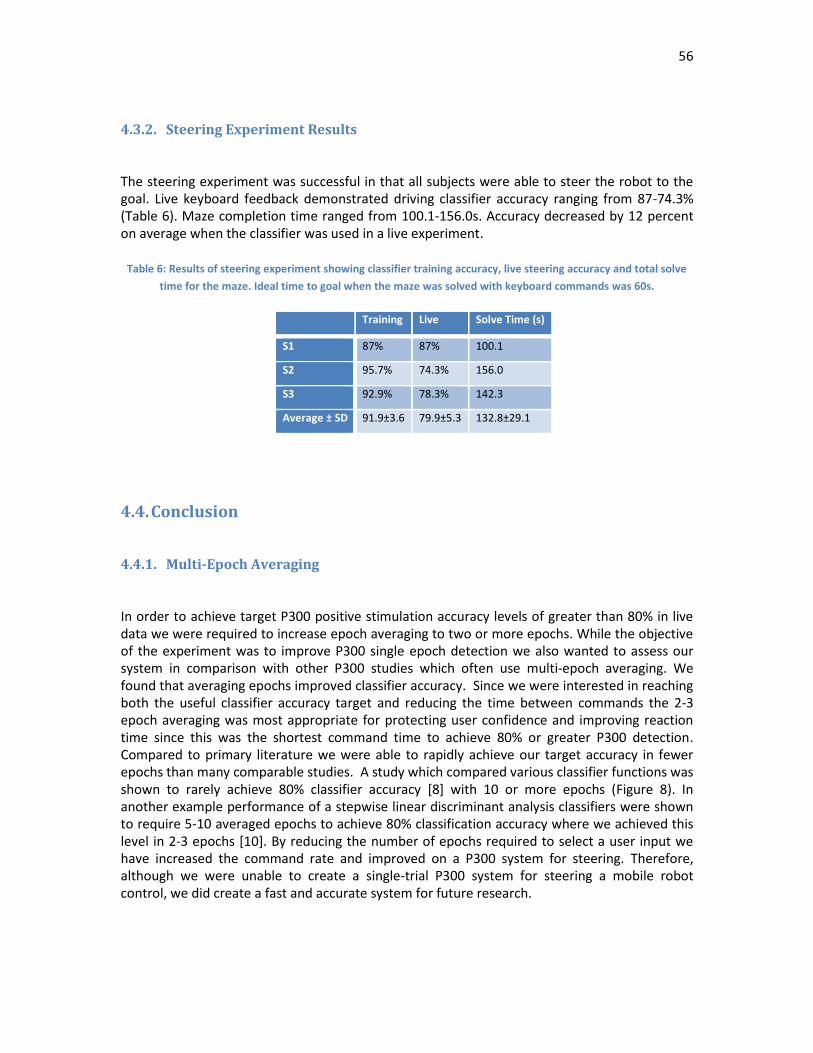
56

4.3.2. Steering Experiment Results

The steering experiment was successful in that all subjects were able to steer the robot to the goal. Live keyboard feedback demonstrated driving classifier accuracy ranging from 87-74.3% (Table 6). Maze completion time ranged from 100.1-156.0s. Accuracy decreased by 12 percent on average when the classifier was used in a live experiment.

Table 6: Results of steering experiment showing classifier training accuracy, live steering accuracy and total solve

time for the maze. Ideal time to goal when the maze was solved with keyboard commands was 60s.

Training Live Solve Time (s)

S1 87% 87% 100.1

S2 95.7% 74.3% 156.0

S3 92.9% 78.3% 142.3

Average ± SD 91.9±3.6 79.9±5.3 132.8±29.1

4.4. Conclusion

4.4.1. Multi-Epoch Averaging

In order to achieve target P300 positive stimulation accuracy levels of greater than 80% in live data we were required to increase epoch averaging to two or more epochs. While the objective of the experiment was to improve P300 single epoch detection we also wanted to assess our system in comparison with other P300 studies which often use multi-epoch averaging. We found that averaging epochs improved classifier accuracy. Since we were interested in reaching both the useful classifier accuracy target and reducing the time between commands the 2-3 epoch averaging was most appropriate for protecting user confidence and improving reaction time since this was the shortest command time to achieve 80% or greater P300 detection. Compared to primary literature we were able to rapidly achieve our target accuracy in fewer epochs than many comparable studies. A study which compared various classifier functions was shown to rarely achieve 80% classifier accuracy [8] with 10 or more epochs (Figure 8). In another example performance of a stepwise linear discriminant analysis classifiers were shown to require 5-10 averaged epochs to achieve 80% classification accuracy where we achieved this level in 2-3 epochs [10]. By reducing the number of epochs required to select a user input we have increased the command rate and improved on a P300 system for steering. Therefore, although we were unable to create a single-trial P300 system for steering a mobile robot control, we did create a fast and accurate system for future research.

57

4.4.2. P300 Steering Experiment

To assess our systems capabilities for use in enabling people with Locked-In syndrome we tested our system with a simulated mobile robot. A multi-epoch classifier was trained to achieve a minimum of 85% positive stimulation classifier accuracy. The results of the experiment show that this system was successful in enabling driving of the simulated robot. All subjects were able to complete the maze in less than 3 minutes. Live classification accuracy remained high despite the additional and novel driving challenge. Although collisions were not recorded we observed that the driver often used walls to stop the robot before they were able to select a new direction. Therefore a real life application of this particular steering system would require some obstacle detection. Obstacle avoidance could also be improved by changing the motion selection system to discrete motion steps rather than motion selections being continual. However, this would require many more user commands and slow the overall task completion time. This is a topic for future exploration and will likely be a reflection of the environment in which the BMI system is operated. For example indoor applications may require more automated obstacle avoidance due to narrow hallways and dynamic obstacles. The advantages of this BMI steering system are the high rate of user commands per second and the simplicity of the design. We hope to demonstrate this process on a mobile robot or wheelchair in the near future.

58

CHAPTER 5 CONCLUSION

5.1. Conclusion

In this chapter results of this thesis are discussed and any contributions of this work are highlighted.

5.1.1. P300 Classifiers

We used three different classifiers to detect P300 signals, the LDA, the NN and the SVM. All techniques were successful in detecting P300 signals. The limited sample size (n=3) of the NN and LDA classifiers prevented statistical comparison between different classifier types. Observations of the results suggest the NN outperformed the LDA in Chapter 2. Similarly, the SVM slightly outperformed the NN in Chapter 3, although not with statistical significance. All classifiers suffered loss of P300 classification accuracy when used on new or live data compared to the training data. This could be due to insufficient training sample size resulting in inaccurate classification assumptions. Another possibility is that over time users respond differently to visual stimuli. Finally, as reported in NN classifier research, over-fitting can result in reduced repeatability of classifier performance. To improve this we recommend exploring increased training sample size. It has been suggested that NN over-fitting can be reduced by adjusting the number of hidden neurons, although this was not explored in our research [24]. Changes in user response to visual stimuli and headset placement are challenges for future research.

Both NN and SVM produce 'black box' classifiers that do not quantify how each feature influences prediction accuracy. This can be limiting in P300 classification analysis as conclusions must be drawn from instances of features selected rather than from a single classifier. For this reason we were required to include 13 participants to increase the statistical power. Although SVM and NN appeared to outperform the LDA, the lack of interpretable output (aside from classification accuracy) reduces the usefulness of these techniques for exploring feature effects.

5.1.2. Genetic Algorithm

The GA was successful in improving feature selection for P300 classification. The GA identified features of the P300 data that are similar to findings from other P300 studies. The most unexpected finding, due statistical probability, was the repeated combination of a single three gene argument in the majority of the GA solutions. This gene described the cross correlation of wave 1 with the 195-391 ms segment from the 01/02 channels subtracted from the T7/T8 channels. The importance of the cross correlation of wave 1 matched the findings of another P300 genetic algorithm study [20]. These results also suggest the GA successfully identified findings common between subjects.

59

The GA also identified the comparison of the occipital and temporal EEG (back-front) electrodes as the channel most influential in identifying P300 signals. This result was interesting as it suggests that re-referencing the channels against electrodes not designated as a reference improved P300 detection. This may be a useful technique for improving performance of low-cost, low SNR ratio EEG headsets such as the Emotiv Epoc. The genetic algorithm did not identify features which were unexpected or not previously described in P300 literature. However, using this algorithm on larger datasets or with higher fidelity EEG systems may identify further population trends.

5.1.3. The Brain Machine Interface

The brain machine interface we constructed was fully capable of recording EEG signals, extracting features with the GA and testing classifiers on live data. One major area of improvement for the system would be adaptive classifier tuning. The GA was responsible for training classifiers with Matlab, and for simplicity only the classification function was transferred to C++ for live testing. The classification function is only a portion of the classifier process, a set of weights and biases that are applied to features. The training portion of the classifier would need to be transferred to C++ for live training in this system. Ideally, a subject would do a short training routine before using the BMI system. With prior knowledge of the subject from initial training with the GA a classifier could be tuned quickly to adapt to minor changes in stimuli amplitude and electrode placement. This could reduce the 10% classifier deterioration observed when we tested an 'old' classifier on new data. Users could also choose to stop and tune a classifier if they were unhappy with performance. This is a development more suitable for long-term users and was therefore not included in our study.

5.1.4. Single-Epoch P300 Detection

Figure 25 shows why single-epoch P300 is an important area of research. Increasing the number of epochs drastically reduces maximum possible bit rates. However, because single-epoch accuracy remains below the ‘useful’ threshold of 80% positive stimulation classification P300, BMI systems continue to require multi-epoch averaging. Therefore more research in single-epoch P300 detection is required. The purpose of this thesis was to explore techniques for improving single-epoch P300 detection and was successful in reducing the number of required epochs to create a useable system.

Results from Chapter 2 and Chapter 3 show that improving selection of temporal, spatial and feature extraction techniques can improve single-epoch P300 detection. More specifically, we suggest that because the correlation of waveform 1 with certain segments of EEG data was common in many of our observed solutions we would suggest creating a user specific wave signal (using training data) to cross correlate with unknown data. Further options for improving single-trial P300 events include hardware development for reducing signal noise, and testing more feature types to broaden the solution space. It may also be possible that the P300 response is not generated consistently enough within a user to reach single-epoch accuracies above 80%. Users can be distracted by the given BMI-task, lose interest, or become tired,

60

resulting in missed stimulations. In live testing we observed that users often went through periods of high accuracy where commands could be selected with ease, while at other times the system was unable to predict the user's desire. Training data, where a user is told which visual stimuli to count, and live testing, where the user selects his, or her, own target, are inherently different tasks. To reduce these challenges we recommend live training or tuning, described in 5.1.3. With live training a user could provide feedback to the system to indicate they were satisfied with the classifier performance and select subsets of training data.

Other options for improving command rate in BMI applications may include changing the displayed stimulation event. In this experiment a neon green rectangle was used to create the visually evoked potential. This may work well in some subjects but less well in others. Auditory cues can also be used to stimulate P300 events [30,12]. We suggest that the genetic algorithm be applied to not only the feature selection process but also to the size, shape, colour, and/or auditory cue used to generate a P300 event.

The difference between a useable single-epoch P300 system and current single-epoch P300 systems is a small but significant amount of classifier accuracy. Although we were unable to develop such a system we believe by that improving and personalizing the visual stimulation, feature extraction, and live classifier tuning, this goal could be achieved in the near future.

5.1.5. P300 Steering of a Simulated Mobile Robot

Using the multi-epoch averaging technique we were able to create a BMI robot steering simulation. All subjects were able to complete the challenge, showing the system was flexible to a variety of users. Command rate was predicted to be 7.5-5.63 commands per minute, similar to other P300 steering studies that achieved 7 commands per minute [27]. Performance of P300 classification suffered during live testing, but we attribute this to the additional task of solving the maze, and repositioning of the EEG headset between training and testing. We would hope to test this system with a live wheelchair as this would bring new challenges in development of a mobile computer system and creating a visual display which could be used on the move. The steering simulation we created also required some automation, the BMI commands were not adequate to avoid occasional collisions with the walls of the maze. This is due in part to the way in which commands were interpreted. Commands, for example forward movement, continued until a new command was given. Using commands for discrete motions, such as forward 3 meters, would reduce the reliance on obstacle avoidance but would also increase solve time and difficulty of the maze. The system was successful in allowing us to test reduced-epoch P300 steering.

61

5.1.6. Contributions

The major contributions of this research can be stated as follows:

1) Identification of novel single-epoch P300 features useful in training P300 classifiers for single subjects and between subjects

2) Construction of a new system for offline training and live testing of P300 3) Creation of a successful P300 steering system with high commands/minute 4) Description of future research required to enable useful single-epoch P300 detection

5.1.7. Future Work

The BMI system developed was successful in validating the experimental results generated by the GA feature selection. Those features improved single-epoch P300 classification and identified techniques to improve low-cost EEG systems. Single-epoch P300 detection is important because lowering epochs required to detect a P300 signal drastically improves bit-rate. Three main areas of improvement suggested which will contribute to the field of P300 classification and enabling victims of LIS. The GA demonstrated the value of wave cross correlation in identifying single-trial P300 signals. These waves should be personalized (shape and time) so that an ideal wave is created from training data for each user. Additionally, electrodes should be re-referenced to increase signal detection. The occipital electrodes compared to the temporal electrodes were particularly useful in P300 detection. Finally, methods of reducing classifier degradation from one sitting to another must be improved. We recommend using an adaptive training system to update classifiers each time the BMI is used. In combination, these three improvements may result in a reliable and accurate single-trial P300 system. By reducing inter-command rates novel P300 systems, such as steering of a wheelchair, will become safer and easier to use.

The new BMI system provides a development platform for future EEG research. The success in improving BMI steering with a low-cost headset should be continued with wheel chair or robotic control. Demonstrating live single-trial or low-trial P300 robot control will represent the state of the art in BMI systems.

62

REFERENCES

[1] E. Donchin, K.M. Spencer, and R. Wijesinghe, "The Mental Prosthesis: Assessing The Speed Of A P300 Based Brain Computer Interface," IEEE Transactions on Rehabilitation Engineering, pp. 174-179, 2000.

[2] S. Sutton, M. Braren, J. Zubin, and E.R John, "Evoked-Potential Correlates Of Stimulus Uncertainty," Science, pp. 1187-1188, 1965.

[3] L.A. Farwell and E Donchin, "Talking Off The Top of Your Head: Toward A Mental Prosthesis Utilizing Event-Related Brain Potentials," Electroencephalography and Clinical Neurophysiology, vol. 70, pp. 510:23, Dec 1988.

[4] I. Iturrate, J.M. Antelis, A. Kubler, and J. Minguez, "A Noninvasive Brain-Actuated Wheelchair Based On A P300 Neurophysiological Protocol And Automated Navigation," IEEE Transactions on Robotics, vol. 25, no. 3, pp. 614:627, June 2005.

[5] C.J. Bell, P. Shenoy, and R. Chalodhorn, "Control Of A Humanoid Robot By Non-Invasive Brain-Computer Interface In Humans," Journal of Neural Engineering, vol. 5, p. 214, June 2008.

[6] K. LaFleur et al., "Quadrotor Control In Three-Dimensional Space Using A Non-Invasive Motor Imagery Based Brain-Computer Interface," Journal of Neural Engineering, vol. 10, June 2012.

[7] J.R. Wolpaw, N. Birbaumer, D.J. McFarland, G. Pfurtscheller, and T.M Vaughan, "Brain-Computer Interfaces For Communication And Control," Journal of Clinical Neurophysiology, vol. 113, pp. 767-791, 2002.

[8] F. Lotte, M. Congedo, A. Lecuyer, F. Lamarche, and B. Arnaldi, "A Review Of Classification Algorithms For EEG-Based Brain-Computer Interfaces," Journal of Neural Engineering, vol. 4, no. 2, June 2007.

[9] M. Duvinage, T. Castermans, and T. Dutoit, "A P300-Based Quantitative Comparison Between The Emotiv Epoc Headset And A Medical EEG Device," in Proceedings of the 9th IASTED international conference on biomedical engineering, June 2012, p. 2.

[10] D.J. Krusienski, E.W. Sellers, D.J. McFarland, T.M. Vaughan, and J.R. Wolpaw, "Toward Enhanced P300 Speller Performance," Journal of Neuroscience Methods, vol. 167, pp. 15-21, August 2008.

[11] R.M. Chapman and H.R. Bragdon, "Evoked Responses To Numerical And Non-Numerical

63

Visual Stimuli While Probem Solving.," Nature, vol. 203, no. 1155-1157, 1964.

[12] E.W. Sellers, D.J. Krusienski, D.J. McFarland, T.M. Vaughan, and J.R. Wolpaw, "A P300 Event-Related Potential Brain-Computer Interface (BCI): The Effects Of Matrix Size And Inter-Stimulus Interval On Performance," Biological Physiology, p. 242, 2006.

[13] J. Kronegg, S. Voloshynovskiy, and T Pun, "Analysis of Bit-Rate Definitions For Brain-Computer Interfaces," in International Conference On Human-Computer Interaction, Las Vegas, 2005, p. 7.

[14] H. Cecotti et al., "Impact Of The Time Segment Analysis For P300 Detection With Spatial Filtering," in 3rd International Symposium on Applied Sciences in Biomedical and Communication Technologies, Rome, 2010, pp. 1-5.

[15] J.V. Tu, "Advantages And Disadvantages Of Using Artificial Neural Networks Versus Logistic Regression For Predicting Medical Outcomes," Journal of Clinical Epidemiology, vol. 49, pp. 1225-1231, November 1996.

[16] D. Albanese. (2012, March) Machine Learning Pythong. website. [Online]. http://mlpy.sourceforge.net/

[17] N. Sharma, "Single-Trial P300 Classification Using PCA and LDA With Neural Networks," 2013.

[18] M. Kaper, P. Meinicke, U. Grossekathoefer, T. Lingner, and H Ritter, "BCI Competition 2003--Data Set IIb: Support Vector Machines for the P300 Speller Paradigm," IEE Transactions in Biomedical Engineering, vol. 51, June 2004.

[19] S. Xie, Y. Wu, Y. Zhang, and C. Liu, "Single Channel Single Trial P300 Detection Using Extreme Learning Machine," in International Joint Conference on Neural Networks, Beijing, 2014.

[20] B. Dal Seno, M. Matteuci, and L. Mainardi, "A Genetic Algorithm For Automatic Feature Extraction In P300 Detection," in International Joint Conference On Neural Networks, Hong Kong, 2008, pp. 3145-3152.

[21] K. Li, R. Sankar, Y Arbel, and E Donchin, "P300 Based Single Trial Independent Component Analysis On EEG Signal," in 5th International Conference on Foundations of Augmented Cognition, Berlin, 2009, pp. 404-410.

[22] S. Silvoni et al., "P300-Based Brain-Computer Interface Communication: Evaluation And Follow-Up In Amyotrophic Lateral Sclerosis," Frontiers of Neuroscience, vol. 3, p. 60, June 2009.

64

[23] D.E. Rumelhart, G.E. Hinton, and R.J Williams, "Learning Representations By Back-Propagating Errors," Nature, vol. 323, pp. 533:536, October 1986.

[24] N. Srivastava, G. Hinton, A. Krizhevsky, I. Sutskever, and R. Salakhutdinov, "Dropout: A Simple Way To Prevent Neural Networks From Overfitting," Journal of Machine Learning Research, vol. 15, pp. 1929-1958, June 2014.

[25] J. Long, Li. Y., T. Yu, and Z. Gu, "Target Selection With Hybrid Feature For BCI-Based 2-D Cursor Control," IEEE Transactions of Biomedical Engineering, vol. 59, pp. 132:40, January 2011.

[26] F. Nijboer et al., "A P300-Based Brain-Computer Interface For People With Amyotrophic Lateral Sclerosis," Journal of Clinical Neurophysiology, vol. 119, pp. 1909-16, August 2008.

[27] G. Pires, M. Castelo-Branco, and U. Nunes, "Visual P300-Based BCI To Steer A Wheelchair: A Bayesian Approach," in 30th Annual International IEEE EMBS Conference, Vancouver, 2008.

[28] C. Escolano, A.M. Murguialday, T. Matuz, N. Birbaumer, and J. Minguez, "A Telepresence Robotic System Operated with a P300-Based Brain-Computer Interface: Initial Tests With ALS Patients," in Annual International Conference of the IEEE Engineering In Medicine and Biology Society, 2010, pp. 4476-4480.

[29] T.J. Sejnowski et al., Toward Brain-Computer Interfacing (Neural Information Processing).: The MIT Press, 2007.

[30] B.H. Jansen et al., "An Exploratory Study Of Factors Affecting Single Trial P300 Detection," IEEE Transactions On Biomedical Engineering, vol. 51, pp. 975-78, June 2004.

[31] D.J. McFarland, W. Sarnacki, and J.R. Wolpaw, "Electroencephalographic (EEG) Control Of Three-Dimensional Movement," Journal of Neural Engineering, vol. 7, no. 3, June 2010.

[32] M. Salvaris and F. Sepulveda, "Visual Modifications On The P300 Speller BCI Paradigm," Journal of Neural Engineering, vol. 6, no. 4, August 2009.

65

APPENDICES

Table A: Instances of repeated segment and operation gene arguments occurring the solution population (n = 60).

Segment (ms)

0-391

391-781

195-586

195-391

391-586

0-586 195-781

78-156

156-234

234-313

313-391

391-469

469-547

547-625

Max 2 0 1 1 0 0 0 2 0 0 0 0 0 0

Min 0 1 0 1 1 0 0 1 0 1 0 0 0 0

Operation PolyCo 0 0 1 5 1 2 0 0 0 0 0 0 0 0

W1 1 0 1 10 0 2 0 2 0 0 0 0 0 2

W2 2 0 0 0 2 0 0 0 0 2 0 1 0 1

W3 0 1 0 0 0 0 1 0 2 1 0 0 1 0

Slope 1 0 0 2 0 2 3 0 0 0 0 0 0 0

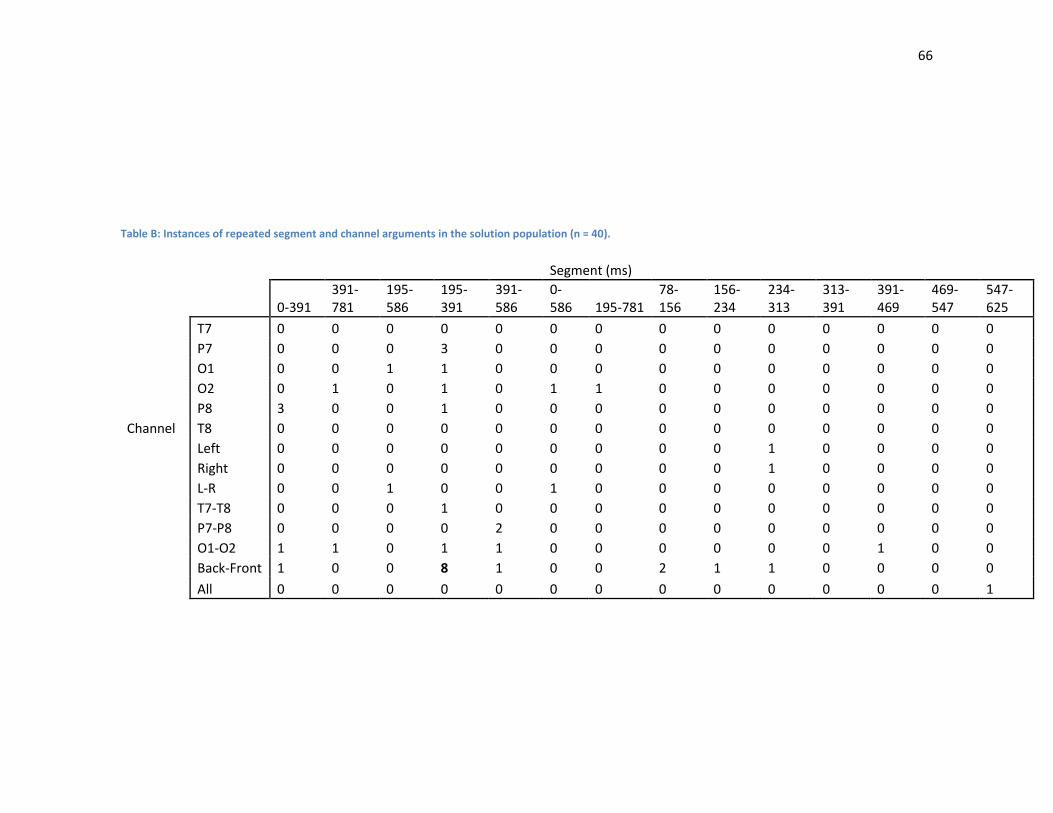
66

Table B: Instances of repeated segment and channel arguments in the solution population (n = 40).

Segment (ms)

0-391

391-781

195-586

195-391

391-586

0-586 195-781

78-156

156-234

234-313

313-391

391-469

469-547

547-625

T7 0 0 0 0 0 0 0 0 0 0 0 0 0 0

P7 0 0 0 3 0 0 0 0 0 0 0 0 0 0

O1 0 0 1 1 0 0 0 0 0 0 0 0 0 0

O2 0 1 0 1 0 1 1 0 0 0 0 0 0 0

P8 3 0 0 1 0 0 0 0 0 0 0 0 0 0

Channel T8 0 0 0 0 0 0 0 0 0 0 0 0 0 0

Left 0 0 0 0 0 0 0 0 0 1 0 0 0 0

Right 0 0 0 0 0 0 0 0 0 1 0 0 0 0

L-R 0 0 1 0 0 1 0 0 0 0 0 0 0 0

T7-T8 0 0 0 1 0 0 0 0 0 0 0 0 0 0

P7-P8 0 0 0 0 2 0 0 0 0 0 0 0 0 0

O1-O2 1 1 0 1 1 0 0 0 0 0 0 1 0 0

Back-Front 1 0 0 8 1 0 0 2 1 1 0 0 0 0

All 0 0 0 0 0 0 0 0 0 0 0 0 0 1

67

Table C: Instances of repeated mathematical operation and channel arguments in the population of solutions.

Operation

Max Min PolyCo W1 W2 W3 Slope

T7 0 1 0 0 0 0 0

P7 0 0 0 4 0 0 0

O1 0 0 0 0 1 1 0

O2 0 0 1 1 0 2 2

P8 1 0 1 1 1 0 1

T8 0 0 0 0 0 0 0

Channel Left 2 0 0 1 1 0 1

Right 0 1 0 1 0 0 0

L-R 0 1 1 0 0 1 0

T7-T8 0 0 0 2 0 0 0

P7-P8 0 0 1 0 1 1 0

O1-O2 2 0 1 1 0 0 4

Back-Front 1 1 5 6 2 1 0

All 0 1 0 0 0 0 0