Fluid Phase Equilibria 232 (2005) 159–170

A generalized regular solution model for asphaltene precipitationfrom n-alkane diluted heavy oils and bitumens

Kamran Akbarzadeh1, Hussein Alboudwarej2,William Y. Svrcek, Harvey W. Yarranton∗

Department of Chemical and Petroleum Engineering, University of Calgary, 2500 University Drive,NW, Calgary, Alta., Canada T2N 1N4

Received 22 September 2004; received in revised form 2 February 2005; accepted 9 March 2005

Abstract

Regular solution theory with a liquid–liquid equilibrium was used to model asphaltene precipitation from heavy oils and bitumens dilutedwith n-alkanes at a range of temperatures and pressures. The input parameters for the model are the mole fraction, molar volume ands fractions:s a molar massd molar massm and pressure-d ipitation fors icted yieldsw ecipitationf©

K

1

ttmdnmamt

, suchoil

recip-nedvent,sport.curateas asure.cipi-nes

ngletta

ntly,ne

xture

0d

olubility parameters for each component. Bitumens were divided into four main pseudo-components corresponding to SARAaturates, aromatics, resins, and asphaltenes. Asphaltenes were divided into fractions of different molar mass based on the gammistribution. The molar volumes and solubility parameters of the pseudo-components were calculated using solubility, density, andeasurements. The effects of temperature and pressure are accounted for with temperature-dependent solubility parametersependent diluent densities, respectively. Model fits and predictions are compared with the measured onset and amount of preceven heavy oil and bitumen samples from around the globe. The overall percent average absolute deviations (%AAD) of the predere less than 1.6% for the diluted heavy oils. A generalized algorithm for characterizing heavy oils and predicting asphaltene pr

rom n-alkane diluted heavy oils at various conditions is proposed.2005 Elsevier B.V. All rights reserved.

eywords: Regular solution; Modeling; Asphaltene precipitation; Heavy oil; Bitumen; Fluid characterization

. Introduction

As conventional oil reserves are depleted, oil sands bi-umen and heavy oil resources are gaining prominence. Bi-umens and heavy oils are rich in asphaltenes; the heaviest,ost polar fraction of a crude oil. Asphaltenes are formallyefined as a solubility class of materials that are insoluble in-alkanes such asn-pentane andn-heptane but soluble in aro-atic solvents such as toluene. Asphaltenes are known to self-ssociate forming aggregates containing approximately 6–10olecules[1,2]. Asphaltenes also contribute significantly to

he high viscosity and the coking tendency of heavy oils and

∗ Corresponding author. Tel.: +1 403 220 6529; fax: +1 403 282 3945.E-mail address:hyarrant@ucalgary.ca (H.W. Yarranton).

1 National Centre for Upgrading Technology, Canada.2 Oilphase-DBR, Canada.

bitumens. In some production and processing schemesas heavy oil upgrading, VAPEX processes or paraffinicsands froth treatment, asphaltenes are deliberately pitated to obtain a lower viscosity and more easily refiproduct. In other cases, heavy oils are diluted with a solsuch as condensate, in order to reduce viscosity for tranTo optimize these processes, it is necessary to have acpredictions of the amount of asphaltene precipitationfunction of the amount of solvent, temperature, and pres

One promising approach to modeling asphaltene pretation is regular solution theory, first applied to asphalteby Hirschberg et al.[3]. They treated asphaltenes as a sicomponent. Kawanaka et al.[4] applied the modified Scoand Maget model[5,6] to asphaltene precipitation usingmolar mass distribution for the asphaltenes. More receYarranton and Masliyah[7] successfully modeled asphalteprecipitation in solvents by treating asphaltenes as a mi

378-3812/$ – see front matter © 2005 Elsevier B.V. All rights reserved.oi:10.1016/j.fluid.2005.03.029

160 K. Akbarzadeh et al. / Fluid Phase Equilibria 232 (2005) 159–170

of components of different density and molar mass. Alboud-warej et al.[8] extended Yarranton and Masliyah’s model andthe Hildebrand and Scott[9,10] regular solution approach toasphaltene precipitation from Western Canadian heavy oilsand bitumens.

The input parameters for the Alboudwarej et al. model[8]were the mole fraction, molar volume and solubility param-eters for each component. Bitumens were divided into fourmain pseudo-components corresponding to SARA fractions:saturates, aromatics, resins, and asphaltenes. Asphalteneswere divided into fractions of different molar mass based onthe gamma molar mass distribution. The extent of asphalteneself-association was accounted for through the average molarmass of the asphaltenes. Correlations for the molar volumesand solubility parameters of the pseudo-components weredeveloped based on solubility, density, and molar mass mea-surements. The preliminary model results for Western Cana-dian bitumens were in good agreement with experimentalmeasurements at ambient conditions. Akbarzadeh et al.[11]extended the model to some heavy oils and bitumens fromaround the globe using the average molar mass of asphaltenesin bitumen as a fitting parameter.

The Alboudwarej et al. model has only been applied at am-bient conditions. In this work, the model is extended to pre-dict asphaltene yields from heavy oils and bitumens dilutedwith n-alkanes over a range of temperatures and pressures.M uredo est-e oils.A tedh

2

sterh Im-p elan Ltd.a TheR Re-s itu-m vy oilw arta,I ment e ColdL odedr d anw plef pro-c d re-c hadb zuelan f ane nesiah sed to

remove water and sand. Toluene,n-heptane,n-pentane, andacetone were obtained from Aldrich Chemical Company andwere 99%+ pure.

Saturates, aromatics, resins, and asphaltenes were ex-tracted from each bitumen or heavy oil according to ASTMD2007M. The molar mass and density of each fraction weremeasured with a Jupiter 833 vapor pressure osmometer andan Anton Paar DMA 46 density meter, respectively. Detailsof the experimental methods are provided elsewhere[11–13].Table 1shows the SARA analysis of heavy oils and bitumens,the density of each fraction at 23◦C, and the molar mass ofeach fraction (measured in toluene at 50◦C).Table 2providesthe measured densities of saturate and aromatic fractions ofan Athabasca sample at various temperatures.

The precipitation of asphaltenes from mixtures of asphal-tene, toluene, and heptane at 0, 23 and 50◦C and from mix-tures of bitumen/heavy oil andn-alkane at 0 and 23◦C wasmeasured in a bench-top apparatus. In addition, asphalteneyields fromn-heptane diluted Athabasca and Cold Lake bi-tumens andn-heptane at various temperatures and pressureswere measured in a mercury-free PVT cell. Details of theexperimental methods are provided elsewhere[12–14].

3. Regular solution model

ud-w –l hase( s) andt po-n as al lud-i .T rest hanea e ex-i ed int ver,s e theb s as-s equi-l y:

K

w olefδ po-np ity

odel fits and predictions are compared with the measnset and amount of asphaltene precipitation for three Wrn Canadian and four international bitumens and heavygeneral approach to predicting precipitation from dilu

eavy oils and bitumens is developed.

. Experimental

Athabasca and Cold Lake bitumens and Lloydmineavy oil were obtained from Syncrude Canada Ltd.,erial Oil Ltd., and Husky Oil Ltd., respectively. Venezuos.1 and 2 bitumens were obtained from Imperial Oilnd DBR Product Center, Schlumberger, respectively.ussia heavy oil was obtained from the Scientific andearch Center for Heavy-Accessible Oil and Natural Ben Reserve in Tatarstan, Russia. The Indonesia heaas obtained from PT. Caltex Pacific Indonesia in Jak

ndonesia. The Athabasca bitumen was an oilsand bituhat had been processed to remove sand and water. Thake and Russia samples were recovered from steam floeservoirs and had also been processed to remove sanater. The Lloydminster heavy oil was a wellhead sam

rom a cyclic steam injection project and had not beenessed. The Venezuela no. 1 bitumen was diluted anovered by naphtha from an underground reservoir andeen processed to remove diluent and sand. The Veneo. 2 sample was a sample collected from a welltest oxploratory well and had not been processed. The Indoeavy oil was a separator sample that had been proces

d

Details of the regular solution model are given in Alboarej et al.[8]. A brief summary is provided here. A liquid

iquid equilibrium is assumed between the heavy liquid pasphaltene-rich phase including asphaltenes and resinhe light liquid phase (oil-rich phase including all coments). It is still not certain that asphaltenes ‘precipitate’

iquid phase or a solid phase. Also, multiple phases, incng V-L1-L2-S, have been observed[15,16] for crude oilsypically, multiple phases appear particularly for mixtuhat either contain very light hydrocarbons, such as metnd ethane, or for systems close to their bubble point. Th

stence or lack of multiple phases in the systems discusshis work could not be confirmed experimentally. Howeince the systems under investigation were well abovubble point and contained no light hydrocarbons, it waumed that there are only two phases at equilibrium. Theibrium ratio,Khl

i , for any given component is then given b

hli = xh

i

xli

= exp

{vhi

vhm

− vli

vlm

+ ln

(vli

vlm

)− ln

(vhi

vhm

)

+ vli

RT(δl

i − δlm)

2 − vhi

RT(δh

i − δhm)

2

}(1)

herexhi andxl

i are the heavy and light liquid phase mractions,R the universal gas constant,T temperature,vi andi are the molar volume and solubility parameter of coment i in either the light liquid phase (l) or the heavy liquidhase (h), andvm andδm are the molar volume and solubil

K. Akbarzadeh et al. / Fluid Phase Equilibria 232 (2005) 159–170 161

Table 1SARA analysis of bitumens and heavy oils and measured molar mass anddensity of each fraction[11]

Fractions wt.% Density (kg/m3) Molar massa (g/mol)

AthabascaSaturates 16.3 900 524Aromatics 39.8 1003 550Resins 28.5 1058 976Asphaltenesb 14.7 1192 7900Solidsc 0.7

Cold lakeSaturates 19.4 882 508Aromatics 38.1 995 522Resins 26.7 1019 930Asphaltenesb 15.5 1190 7400Solidsc 0.3

LloydminsterSaturates 23.1 876 482Aromatics 41.7 997 537Resins 19.5 1039 859Asphaltenesb 15.3 1181 6660Solidsc 0.4

Venezuela 1Saturates 15.4 885 447Aromatics 44.4 1001 542Resins 25.0 1056 1240Asphaltenesb 15.0 1186 10005Solidsc 0.2

Venezuela 2Saturates 20.5 882 400Aromatics 38.0 997 508Resins 19.6 1052 1090Asphaltenesb 21.8 1193 7662

Solidsc 0.1

RussiaSaturates 25.0 853 361Aromatics 31.1 972 450Resins 37.1 1066 1135Asphaltenesb 6.8 1192 7065Solidsc 0.0

IndonesiaSaturates 23.2 877 498Aromatics 33.9 960 544Resins 38.2 1007 1070Asphaltenesb 4.7 1132 4635Solidsc 0.0

a For asphaltenes the corrected molar mass at 23◦C is 20% higher thanthe measured value at 50◦C [19].

b Asphaltenes average molar mass measured at 50◦C and 10 kg/m3 intoluene.

c Non-asphaltic solids.

Table 2Densities of saturate and aromatic fractions of an athabasca bitumen sample

Temperature (◦C) Density (kg/m3)

Saturates Aromatics

15 895.1 –25 888.8 1006.435 – 1004.040 879.2 996.655 869.6 –

parameter of either the light liquid phase or the heavy liquidphase. Note that the above formulation is equivalent to asolid–liquid phase equilibrium where the contribution of theheat of fusion to the equilibrium expression is negligible.

It was assumed that only asphaltenes and resins partitionedto the heavy phase. In reality, all the fractions could poten-tially partition; however, allowing all components to parti-tion significantly increases the time for the model to con-verge. Furthermore, experimental observations indicate thatthe heavy phase consists primarily of asphaltenes and resins.Once the equilibrium ratios are known the phase equilibriumis determined using standard techniques[8,17].

4. Fluid characterization

The first step in fluid characterization is to divide thefluid into components and pseudo-components. In this case,each solvent is an individual component with known prop-erties. The bitumen or heavy oil was divided into pseudo-components based on SARA fractions (saturates, aromatics,resins, and asphaltenes). The saturates, aromatics, and resinswere each treated as a single pseudo-component. However, itproved necessary to divide the asphaltene fraction into severalpseudo-components in order to accurately predict yields.

The asphaltenes are here considered to be macromolec-u mers.T udo-c utionf ibu-t

f

w rage‘ rw olarm er ad

f

w d isd

r

T ver,s , them sed in

lar aggregates of monodisperse asphaltene monoherefore, the asphaltene fraction was divided into pseomponents based on molar mass. The gamma distribunction [18] was used to describe the molar mass distrion:

(M) = 1

Γ (β)

[β

(M − Mm)

]β

× (M − Mm)β−1

× exp

[β(M − Mm)

(M − Mm)

](2a)

hereMm, andM are the monomer molar mass and aveassociated’ molar mass of asphaltenes, andβ a parametehich determines the shape of the distribution. Since mass is an intrinsic property, it is preferable to considistribution of aggregation numbers given by:

(r) = 1

MmΓ (β)

[β

(r − rm)

]β

× (r − rm)β−1

× exp

[β(r − rm)

(r − rm)

](2b)

herer is the number of monomers in an aggregate anefined as follows:

= M

Mm

(2c)

his formulation was used in the modeling work. Howeince the monomer molar mass is not well establishedeasured apparent or associated molar masses are u

162 K. Akbarzadeh et al. / Fluid Phase Equilibria 232 (2005) 159–170

the following discussion. As discussed elsewhere[8], the as-phaltenes were discretized into 30 fractions ranging up to30,000 g/mol. The asphaltene monomer molar mass was as-sumed to be 1800 g/mol. The average aggregation number (orassociated asphaltene molar mass) depends on the composi-tion and temperature[17] and must be measured or estimatedfor any given condition.

The value ofβ is unknown although a value of 2 is rec-ommended for polymer systems. However, the extent ofasphaltene self-association and hence the asphaltene mo-lar mass distribution depend on temperature. Therefore,the parameterβ was also assumed to be temperature de-pendent. The following correlation forβ was determinedby fitting the model to precipitation data for mixtures ofasphaltene–heptane–toluene at temperatures of 23 and 50◦C,as shown inFig. 1:

β(T ) = −0.0259T + 10.178 (3)

whereT is the temperature in Kelvin. Note that the corre-lation has only been tested for temperatures between 0 and100◦C and cannot apply at temperatures exceeding 120◦Cbecause the predictedβ decreases below zero. More data athigher temperatures is required to extend the correlation ap-propriately.

ulars vol-u molef re de-t , theS sses.M n de-t

F ns ofn

Table 3Average molar masses, densities, and solubility parameters of saturates, aro-matics, and resins

Fraction Molar Mass at50◦C (g/mol)

Density at23◦C (kg/m3)

Solubility parameterat 23◦C (MPa)0.5

Saturates 460 880 15.9Aromatics 522 990 20.2Resins 1040 1044 19.6

4.1. Molar volumes

The molar volumes of the solvents were calculated usingHankinson–Brobst–Thomson (HBT) technique[20], whichaccounts for both the effect of temperature and pressure. Themolar volumes of the saturates and the aromatics can be de-termined either from the individual measured molar massesand densities for fractions from each bitumen or heavy oil,given inTable 1, or from the average molar masses and den-sities given inTable 3. The average properties are used in thiswork.

The data fromTable 2was used to determine the tem-perature dependence of the densities. The following curvefit equations were found for the densities of the saturate andthe aromatic fractions of an Athabasca bitumen sample as afunction of temperature:

ρsat = −0.6379T + 1078.96 (4)

ρaro = −0.5942T + 1184.47 (5)

whereρsat andρaro are the densities of Athabasca saturatesand aromatics in kg/m3, respectively. It was assumed that thechange in density with temperature was the same for satu-rates and aromatics extracted from any heavy oil/bitumen.Hence, the correlations were modified as follows to matchthe average density of saturates and aromatics fromTable 3b

ρ

ρ

w anda nK

e de-t larm

ρ

wt ltenef .N getherb cleara witht e as-p ssed

The second step in the fluid characterization for regolution models is to determine the mole fraction, molarme, and solubility parameter of each component. The

ractions of the components and pseudo-components aermined from the masses of the solvent and bitumenARA analysis, and the measured or estimated molar maolar volumes and solubility parameters are discussed i

ail below.

ig. 1. Fractional precipitation of Athabasca asphaltenes from solutio-heptane and toluene at 0, 23, and 50◦C.

ut retain the slopes from Eqs.(4) and (5):

sat = −0.6379T + 1069.54 (6)

aro = −0.5943T + 1164.73 (7)

hereρsatandρaro are the average densities of saturatesromatics in kg/m3, respectively andT the temperature ielvin.

The molar volumes of the asphaltenes and resins arermined from the following correlation of density to moass[8]:

= 670M0.0639 (8)

hereρ is the asphaltene or resin density in kg/m3 andMhe molar mass in g/mol. The molar mass of an aspharaction is the associated molar mass (rMm) of that fractionote that the asphaltenes and resins are considered toecause they are assumed to be a continuum of polynuromatics. The change in asphaltene average density

emperature is accounted for with the change in averaghaltene molar mass with temperature, as will be discu

K. Akbarzadeh et al. / Fluid Phase Equilibria 232 (2005) 159–170 163

later. It was assumed that the change in density of the SARAfractions with pressure was negligible.

4.2. Solubility parameters

The solubility parameter is defined as follows:

δ =(

�Hvap − RT

ν

)1/2

(9)

where�Hvap is the heat of vaporization. The solubility pa-rameters of the solvents can be determined from existing cor-relations of heats of vaporization and molar volumes. How-ever, the model predictions are very sensitive to small changesin the solubility parameter and an estimation of the sol-vent solubility parameter with an accuracy of approximately±0.05 MPa0.5 is necessary. In this work, the following ap-proach was found to give good predictions of the asphalteneyields.

First, the heats of vaporization were calculated using theDaubert et al. correlation[21]. Then, the molar volumes weredetermined using the HBT technique[20]. The solubility pa-rameters obtained using these correlations and Eq.(9) agreewith the literature values[22] for n-heptane at different tem-peratures and forn-hexane andn-pentane at 25◦C, as showni dona ubil-i ture[ s forn

δ

wa angei r allo cor-r

TS

S

n

n

n

at different temperatures:

δs,T = δs,25 − 0.0232(T − 298.15) (11)

whereδs,T is solvent solubility parameter at temperatureT,δs,25 is solvent solubility parameter at 25◦C estimated fromEq.(9), andT the temperature in K. The predicted solubilityparameters are compared with literature values inTable 4.The effect of pressure on the solvent solubility parametersis accounted for in the decrease in their molar volume withpressure.

The heats of vaporization of SARA fractions cannot bedetermined because the fractions decompose below the boil-ing point. Instead, the solubility parameters were determinedby fitting the model to asphaltene solubility data for mixturesof asphaltenes and solvents.

The solubility parameter of the asphaltenes (and resins)was determined from the following correlation of solubil-ity parameter to density recommended by Yarranton andMasliyah[7]:

δa =[�Hvap − RT

v

]1/2

=[

r�Hvapm − RT

rMm/ρ

]1/2

=[(

�Hvapm

Mm

− RT

rMm

)ρ

]1/2

≈ (A(T ) ρ)1/2 (12)

w sa por-i ggre-g pies,t y thep heato em t wasa samea there-f in-c s, thea a thed sumedt pa-r

wingc re-c uenea

A

w m-e m-p lp In-c hef qs.( ted

n Table 4. However, the predicted solubility parametersot match the literature values forn-hexane andn-pentanet 0◦C. Therefore, an alternate method was applied. Sol

ty parameters are expected to vary linearly with tempera22]; and, therefore, the calculated solubility parameter-heptane were plotted versus temperature to obtain:

h = 22.121− 0.0232T (10)

hereδh is the solubility parameter ofn-heptane in (MPa)0.5

ndT the temperature in K. It was assumed that the chn solubility parameter with temperature was the same fof then-alkanes considered here. Hence, the followingelation was found for the solubility parameter ofn-alkanes

able 4olubility parameters ofn-alkanes at various temperatures

olvent Temperature (◦C) Solubility parameter (MPa0.5)

Eq.(7) Eq.(9) Ref. [22]

-Heptane 0 15.81 15.80 15.9025 15.20 15.20 15.2045 14.70 14.74 14.7560 14.31 14.39 14.41

100 13.50 13.50 13.59

-Hexane 0 15.55 15.46 15.4225 14.88 14.88 14.8145 14.31 14.41 14.5060 13.87 14.07 14.20

-Pentane 0 15.15 14.95 15.0025 14.37 14.37 14.3545 13.71 13.91 13.81

hereδa is the solubility parameter (MPa0.5) of asphaltenendA is approximately equal to the monomer heat of va

zation (kJ/g). (Since asphaltenes are considered to be aates of monomers with relatively low association enthal

he heat of vaporization of an aggregate is approximatelroduct of the number of monomers and the monomerf vaporization. The termRT/rM is much smaller than thonomer heat of vaporization and can be neglected.) Issumed that the heat of vaporization of a resin was thes that of an asphaltene monomer on a mass basis and

ore Eq.(12) is applied to resins as well. The correlationorporates the effect of temperature and, for asphalteneggregation number of the given asphaltene fraction viensity. Since the asphaltene and resin densities are as

o be independent of pressure, their calculated solubilityameters are also independent of pressure.

Parameter A depends on the temperature. The folloorrelation forA was determined by fitting the model to pipitation data for mixtures of asphaltene–heptane–tolt temperatures of 23 and 50◦C as shown inFig. 1:

(T ) = −6.667× 10−4T + 0.5614 (13)

hereT is the temperature in Kelvin. Note that two paraters (β andA) were fitted to account for the effect of teerature. Increasing the magnitude ofA shifted the fractionarecipitation curve to lower heptane volume fractions.reasing the magnitude ofβ led to a steeper slope on tractional precipitation curve. To test the correlations (E3) and (13)), the fractional precipitation curve was predic

164 K. Akbarzadeh et al. / Fluid Phase Equilibria 232 (2005) 159–170

Fig. 2. Fractional precipitation of Athabasca asphaltenes from solutions ofn-heptane/aromatics and saturates/toluene at 23 and 50◦C.

for 0◦C. Fig. 1shows that the predicted fractional precipita-tion agrees well with the data.

Fig. 2 shows asphaltene precipitation data for mixturesof asphaltenes, saturates, and toluene as well as asphaltenes,n-heptane, and aromatics at 23 and 50◦C. The saturates andaromatics solubility parameters found to fit the data are givenin Table 5and the corresponding model predictions are shownonFig. 2. The solubility parameters inTable 5differ slightlyfrom those used in previous work[8,11] because additionalsolubility data was obtained allowing for a more accuratecalculation. The following correlations were developed toestimate the solubility parameters of saturates and aromaticsat different temperatures:

δsat = 22.381− 0.0222T (14)

δaro = 26.333− 0.0204T (15)

whereδsat andδaro are the solubility parameters of saturatesand aromatics in MPa0.5 and T the temperature in Kelvin.The saturate and aromatic solubility parameters are assumedto be independent of pressure.

Akbarzadeh et al.[11] showed that using the average val-ues of density, molar mass, and solubility parameter for theSARA fractions provided inTable 3, rather than the individualvalues for each oil inTable 1, did not affect the model pre-dictions significantly. To retain the generality of the model,t hesea

TF

F

SA

5. Results and discussion

Once the fluid characterization was completed, only oneunknown parameter remained: the average associated molarmass (¯rMm) of the asphaltenes in the bitumen or heavy oil.This parameter is temperature and source dependent becauseasphaltene association is temperature and source dependent.In general, smaller average molar masses expected at highertemperatures and in fluids with high resin content[2]. Thefollowing approach was taken to finalize the model:

1. The average associated asphaltene molar mass at 23◦Cwas determined by fitting the model to asphaltene yieldsfromn-heptane diluted bitumens and heavy oils at ambientconditions.

2. The temperature dependence of the average associated as-phaltene molar mass was determined by fitting the modelto asphaltene yields fromn-heptane diluted Athabasca bi-tumen at various temperatures.

3. The model was tested on different bitumens and heavy oilsdiluted withn-pentane,n-hexane,n-heptane, orn-octaneat various temperatures and pressures.

4. A generalized modeling approach is recommended for:(a) cases with some experimental yield data (average as-sociated asphaltene molar mass is a fitting parameter); (b)cases with no experimental data (no adjustable parame-

5m

avyot Inter-e ation

Fh

he model predictions in this work are also based on tverage values.

able 5itted solubility parameters for saturates and aromatics at 23 and 50◦C

raction Fitted solubility parameter (MPa)0.5

23◦C 50◦C

aturates 15.9 15.25romatics 20.2 19.7

ters).

.1. Fitting the average asphaltene associated molarass at 23◦C

Fig. 3 shows the asphaltene yields from various heils/bitumens upon dilution withn-heptane (n-pentane in

he case of Indonesian sample) at ambient conditions.stingly, the experimental onset of asphaltene precipit

ig. 3. Fractional yield of precipitate from various oils diluted withn-eptane (orn-pentane for Indonesian oil) at 23◦C.

K. Akbarzadeh et al. / Fluid Phase Equilibria 232 (2005) 159–170 165

Table 6Fitted asphaltene molar mass in heavy oils/bitumens and average absolutedeviation (AAD)a for different systems

Bitumen/heavyoil

Fitted asphaltenemolar mass, M23

(g/mol)

%AADb

n-Heptane n-Hexane n-Pentane

Athabasca 2965 0.534 0.494 0.705Cold Lake 2990 0.855 0.508 0.937Lloydminster 3005 0.522 0.690 0.552Venezuela no. 1 3000 0.757 – 0.707Venezuela no. 2 3025 0.690 – 0.883Russia 2800 0.436 – 0.496Indonesia 2270 – – 0.623

a %AAD = 100× (ΣN |calculated− experimental|/N).b Based on average properties for saturates, aromatics, and resins presented

in Table 3.

occurs at approximately the same heptane content(54± 4 wt.%) for all of the heptane diluted crude oils eventhough the ultimate yields vary significantly. Hence, it ap-pears that the onset of precipitation does not depend sig-nificantly on the asphaltene content of the oil. Perhaps, theasphaltene molar mass distribution is the more significantfactor in determining the onset point.

The fitted average molar mass for each system is providedin Table 6. All of the average molar masses are within 1.2%of 3000 g/mol except for the Russian and Indonesian sam-ple. The Russian and Indonesian crude oils have the highestresin-to-asphaltene mass ratio (R/A ratio) of all the crude oils.The extent of asphaltene association is known to decrease asthe ratio of resins to asphaltenes increases[2]. Therefore,the calculated average asphaltene molar masses were plottedagainst theR/A ratio of each crude oil, as shown inFig. 4.Most of the data is clustered and only two points correspond-ing to the Russian (R) and Indonesian (I) samples are spreadout sufficiently to discern a clear trend. Nonetheless, the cal-culated molar mass decreases as theR/A ratio increases and

F resin-t ster,V .

Fig. 5. Effect of temperature on the yield of precipitation from Athabascabitumen diluted withn-heptane; data at 50 and 100◦C from[14].

decreases dramatically above anR/Aratio of approximately 5.The following third degree polynomial fits the data ofFig. 4:

M23 = −3.207(R/A)3 + 25.943(R/A)2 − 101.04(R/A)

+ 3099.4 (16)

whereM23 is the average molar mass of asphaltenes in heavyoils/bitumens at 23◦C in g/mol.

However, more data over a wide range ofR/A ratio arerequired to test the applicability of the correlation.

5.2. Fitting the temperature dependence of the averageasphaltene molar mass

The model was fitted to Athabasca bitumen/n-heptane sys-tem at 0, 23, 50, and 100◦C, as shown inFig. 5. The fittedmolar masses are given inTable 7. The form of the tem-perature dependence of the average asphaltene molar mass isunknown. However, the data were observed to follow a lineartrend versus temperature and were fitted with the followingequation:

MT,ath = −10.599T + 6043.523 (17)

whereMT,ath is the average molar mass of asphaltenes inAthabasca bitumen in g/mol at temperatureT in K.

TF ratures

T l)

1

ig. 4. The fitted asphaltene molar mass in bitumen versus the

o-asphaltene ratio. Ath = Athabasca, CL = Cold Lake, LM = Lloydmin1 = Venezuela no. 1, V2 = Venezuela no. 2, R = Russia, I = Indonesia

able 7itted asphaltene molar mass in Athabasca bitumen at various tempe

emperature (◦C) Fitted molar mass (g/mo

0 310023 296050 263000a 2070a Pressure = 2.07 MPa.

166 K. Akbarzadeh et al. / Fluid Phase Equilibria 232 (2005) 159–170

It was assumed that the change in average asphaltene mo-lar mass with temperature was the same for all of the crudeoils. Hence, the following general correlation is suggested forthe temperature dependency of the average asphaltene molarmass:

MT = M23 − 10.599(T − 296.15) (18)

whereMT is the average molar mass at temperatureT, M23the average molar mass at 23◦C reported inTable 6, andTthe temperature in Kelvin.

5.3. Model predictions

5.3.1. Solvent effectOnce the average molar mass of asphaltenes in heavy

oil/bitumen was determined, the model can be used to predictthe onset and amount of precipitation from heavy oil/bitumendiluted with othern-alkanes with no other adjustment.Fig. 6shows the asphaltene yields from Lloydminster heavy oilupon dilution with variousn-alkanes at ambient conditions.The model was fitted to the heptane diluted data using anaverage asphaltene molar mass of 3005 g/mol giving an av-erage percent absolute deviation (%AAD) of 0.27%. Themodel successfully predicted the onset of precipitation andasphaltene yields for the heavy oil/n-pentane,n-hexane, andn -a d foro ntc

s entd he eta ita-t mber

F tedw

of the diluent increased up to 8–10 but then decreases at stillhigher carbon numbers. In other words, heptane is a bettersolvent than pentane but dodecane is a better solvent thandecane. They also showed that this model correctly predictedthe observed trend. Hence, the predicted in increase in as-phaltene yield withn-octane diluent is likely the same trendemerging for the Lloydminster oil.

Also note that, in almost all the diluted bitumens, the as-phaltene yield calculated from the model decreases at highn-alkane mass fractions while the experimental data level off orcontinue to increase with a small slope. The predicted yieldsdecrease because the solutions are becoming dilute in bitu-men and asphaltenes and a small asphaltene solubility beginsto affect the yield. The reason this effect is not observed in thedata may be that asphaltenes self-associate to a greater extentas the diluent content increases. Increasing self-associationwould decrease asphaltene solubility and oppose the dilutioneffect.

5.3.2. Temperature effectFigs. 7–13show model predictions for asphaltene pre-

cipitation, respectively, from Athabasca bitumen, Cold Lakebitumen, Lloydminster heavy oil, Venezuela no. 1 bitumen,Venezuela no. 2 bitumen, Russia heavy oil, and Indonesiaheavy oil diluted with variousn-alkanes at various tem-p thea e pre-s tedt an1

lr a. Iti lieso ures

F mend

-octane solutions. The overall %AAD for Lloydminstern-lkane systems is 0.46%. Similar results were obtainether heavy oils/bitumens diluted withn-alkanes at ambieonditions[11].

Note that the predicted asphaltene yields in then-octaneystem are higher than that in then-heptane system evhough the experimental yields forn-octane andn-heptaneilution are the same within the scatter of the data. Wiel. [23] showed forn-alkane diluents, the onset of precip

ion occurs at higher diluent content as the carbon nu

ig. 6. Fractional yield of precipitate from Lloydminster bitumen diluith n-alkanes at ambient conditions; data from[8].

eratures. The total %AAD’s for predictions based onverage properties and the suggested correlations arented inTable 6. In almost all cases, the model prediche amount of precipitation with a %AAD of less th%.

There is only one data set at 100◦C,Fig. 8, and the modeesults do not match very well with the experimental dats possible that a liquid–liquid equilibrium no longer appr that the property correlations begin to fail at temperat

ig. 7. Predicted fractional yield of precipitate from Athabasca bituiluted withn-pentane andn-hexane at 0 and 23◦C.

K. Akbarzadeh et al. / Fluid Phase Equilibria 232 (2005) 159–170 167

Fig. 8. Predicted fractional yield of precipitate from Cold Lake bitumendiluted withn-pentane andn-heptane at various temperatures; data at 50 and100◦C from[14].

as high as 100◦C. On the other hand, there were some dif-ficulties in obtaining consistent experimental data at 100◦C[14]. At this stage, it is not clear if the problem is with themodel or the data.

At 0 ◦C the model under-predicted the ultimate amountof precipitation for most of heavy oils and bitumens di-luted with n-pentane. One possible explanation for under-prediction is that at temperatures as low as 0◦C, resins mayself-associate in a similar mechanism to asphaltenes. To ac-count for self-association of resins in the model, the gammadistribution function (Eqs.(2a) and (2c)) was used to divideresins into five fractions based on the molar mass ranging up

F y oild

Fig. 10. Predicted fractional yield of precipitate from Venezuela no. 1 bitu-men diluted withn-pentane andn-heptane at various temperatures; data at23◦ from [11].

to 1900 g/mol. The resin monomer molar mass was assumedto be 200 g/mol. The average resin molar mass was assumedconstant at 1040 g/mol as given inTable 3. Fig. 14comparesmodel predictions with and without resin precipitation forAthabasca and Russia samples diluted withn-pentane at 0◦C.The model predictions for Athabasca system are improved ifresins are indeed self-associating and the self-association istaken into account. However, at this stage, there is insufficientsupporting evidence to incorporate resin self-association intothe model.

F bitu-m ta at2

ig. 9. Predicted fractional yield of precipitate from Lloydminster heaviluted withn-pentane andn-heptane at various temperatures.

ig. 11. Predicted fractional yield of precipitate from Venezuela no. 2en diluted withn-pentane andn-heptane at various temperatures; da3◦ from [11].

168 K. Akbarzadeh et al. / Fluid Phase Equilibria 232 (2005) 159–170

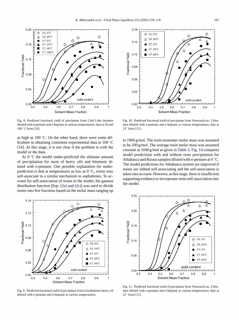
Fig. 12. Predicted fractional yield of precipitate from Russia heavy oil di-luted with n-pentane andn-heptane at various temperatures; data at 23◦Cfrom [11].

5.3.3. Pressure effectThe effect of pressure on asphaltene precipitation from

Athabasca bitumen and Cold Lake bitumen is shown inFigs. 15 and 16, respectively. Although the only pressuredependency considered in the model is with the molar vol-ume of the solvents, the model could accurately predict theamount of precipitation at moderate pressures (e.g. 2.1 MPa).However, the model under-predicted the ultimate amount ofprecipitation at high pressures (e.g. 6.9 MPa). Accountingfor the effect of pressure on the pseudo-component parame-ters could improve the model predictions especially at high

F y oild

Fig. 14. Predicted fractional yield of precipitate from Athabasca and Rus-sia samples diluted withn-pentane at 0◦C with and without resin self-association.

pressures. Nonetheless, the %AADs of the model predictionswere less than 1.6% in all cases.

5.4. Generalized model

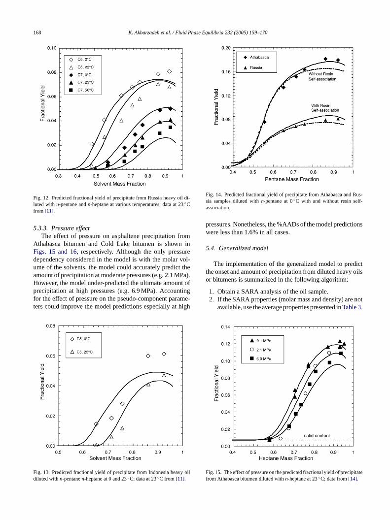
The implementation of the generalized model to predictthe onset and amount of precipitation from diluted heavy oilsor bitumens is summarized in the following algorithm:

1. Obtain a SARA analysis of the oil sample.2. If the SARA properties (molar mass and density) are not

available, use the average properties presented inTable 3.

F pitatef

ig. 13. Predicted fractional yield of precipitate from Indonesia heaviluted withn-pentanen-heptane at 0 and 23◦C; data at 23◦C from[11].

ig. 15. The effect of pressure on the predicted fractional yield of precirom Athabasca bitumen diluted withn-heptane at 23◦C; data from[14].

K. Akbarzadeh et al. / Fluid Phase Equilibria 232 (2005) 159–170 169

Fig. 16. The effect of pressure on the predicted fractional yield of precipitatefrom Cold Lake bitumen diluted withn-heptane at 23◦C; data from[14].

Calculate the densities of saturates and aromatics at tem-peratures other than 23◦C from Eqs.(6) and (7).

3. Estimate solubility parameters of saturates and aromaticsfrom Eqs.(14) and (15).

4. Estimate the average molar mass of asphaltenes at 23◦Cfrom Eq. (16) and at the desired temperature from Eq.(18).

5. Subdivide asphaltenes (and resins if desired) using theGamma distribution (Eqs.(2a), (2c) and (3)).

6. Determine densities and solubility parameters of asphal-tene and resin sub-fractions from Eqs.(8), (12) and (13).

7. Calculate the liquid molar volumes and solubility param-eters of the relevantn-alkane(s) from Hankinson-Brobst-Thomson (HBT) technique[18] and Eqs.(9) and (11),respectively.

8. Perform equilibrium calculations using Eq.(1) and stan-dard techniques[8,15]. A bisection method may be re-quired to converge the model.

9. Calculate the amount of precipitation at desired condi-tions (temperature, pressure, solvent mass fraction).

10. Check the accuracy of model predictions with experi-mental data if available. If necessary, adjust the averageasphaltene molar mass to obtain a better fit.

The proposed asphaltene precipitation model is valid fora heavy oils and bitumens diluted with liquidn-pentane andh up to1 asedo e ofc itioni be-y them ctive.I teps

1–9. A more accurate solution may be obtained if the averagemolar mass is tuned to fit some data.

6. Conclusions

Seven bitumens/heavy oils were characterized in terms ofSARA fractions. The molar volume and solubility parameterof the fractions were determined from molar mass, density,and asphaltene precipitation measurements. Since the molarmass of asphaltenes in bitumen is unknown, it was estimatedby fitting the proposed regular solution model to precipitationdata from solutions of bitumen andn-heptane at ambient con-ditions. A correlation was developed to estimate the averagemolar mass of asphaltenes in heavy oils and bitumens usingthe resin-to-asphaltene ratio. Asphaltene yields were mod-eled forn-alkane diluted bitumens and heavy oils at varioustemperatures from 0 to 100◦C and pressures up to 7 MPa.The fitted and predicted onset and amount of precipitationwere in reasonable agreement with the experimental data inmost cases. In all cases, the percent average absolute devi-ations (%AAD) of the predicted yields were less than 1.6%for the diluted heavy oils and bitumens.

List of symbolsA parameter in Eq.(12)AfKMPr teRRTv

x

Gβ

δ

�

Γ

ρ

S22aaahimrs

igher carbon number alkanes at temperatures from 000◦C and pressures up to 7 MPa. Since the model is bn property correlations determined for only this rangonditions and because only a liquid–liquid phase transs considered, caution is recommended in extrapolatingond these conditions. Within this range of conditions,odel is predictive in the same sense an EoS is predi

t can provide an approximate solution if run using the s

AD average absolute deviationmass frequencyequilibrium ratiomolar mass (g/mol)pressure (MPa)number of monomers in an asphaltene aggregauniversal gas constant (cm3 bar/mol K)

/A resin-to-asphaltene mass ratio (wt./wt.)temperature (K)molar volume (cm3/mol)mole fraction

reek symbolsparameter in gamma distribution functionsolubility parameter (MPa)0.5

Hvap heat of vaporization (J/mol)gamma functiondensity (kg/m3)

ubscripts3 at 23◦C5 at 25◦C

asphaltenesro aromaticsth Athabasca

heptanei -th componentmonomerresinssolvent

170 K. Akbarzadeh et al. / Fluid Phase Equilibria 232 (2005) 159–170

T at temperatureTsat saturates

Superscriptsh heavy phasel light phase

Acknowledgements

Financial support from the Natural Sciences and Engineer-ing Research Council of Canada (NSERC) and the AlbertaEnergy Research Institute (AERI) is appreciated. The authorsalso thank Syncrude Canada Ltd., Imperial Oil Ltd., HuskyOil Ltd., DBR Product Center, Schlumberger, the Scientificand Research Center for Heavy-Accessible Oil and NaturalBitumen Reserve in Tatarstan, and PT. Caltex Pacific Indone-sia for supplying oil samples.

References

[1] J.G. Speight, The Chemistry and Technology of Petroleum, 3rd ed.,Marcel Dekker, New York, 1999.

[2] M. Agrawala, H.W. Yarranton, Asphaltene association model anal-ogous to linear polymerization, Ind. Eng. Chem. Res. 40 (2001)4664–4672.

nce(1984)

fromRes.

olu-of

.olu-ge-

bil-

an-bitu-

[9] J. Hildebrand, R. Scott, Solubility of Non-Electrolytes, 3rd ed., Rein-hold, New York, 1949.

[10] J. Hildebrand, R. Scott, Regular Solutions, Prentice-Hall, EnglewoodCliffs, NJ, 1962.

[11] K. Akbarzadeh, A. Dhillon, W.Y. Svrcek, H.W. Yarranton, Method-ology for the characterization and modeling of asphaltene precipita-tion from heavy oils diluted withn-alkanes, Energy Fuels 18 (2004)1434–1441.

[12] H. Alboudwarej, K. Akbarzadeh, J. Beck, W.Y. Svrcek, H.W. Yarran-ton, Sensitivity of asphaltene properties to extraction techniques, En-ergy Fuels 16 (2002) 462–469.

[13] K. Akbarzadeh, O. Sabbagh, J. Beck, W.Y. Svrcek, H.W. Yarran-ton, Asphaltene precipitation from bitumen diluted withn-alkanes,in: Proceedings of the Canadian International Petroleum Confer-ence, CIPC paper no. 2004-026, June 8–10, Calgary, Canada,2004.

[14] H. Alboudwarej, Asphaltene deposition in flowing system. Ph.D.Thesis, University of Calgary, Calgary, Alta., Canada, April 2003.

[15] J.L. Shelton, L. Yarborough, Multiple phase behavior in porous me-dia during CO2 or rich-gas flooding, JPT (SPE #5827), September1977, 1171–1178.

[16] J.M. Shaw, T.W. deLoos, J. de Swaan Arons, An explanation forsolid–liquid–liquid–vapour phase behaviour in reservoir fluids, Pet.Sci. Technol. 15 (1997) 503–521.

[17] M.P.W. Rijkers, R.A. Heidemann, in: K.C., Chao, R.L., Robin-son, Jr., (Eds.), Convergence behavior of single-stage flash calcu-lations, Article in Equations of State, Proceedings of the Theoriesand Applications ACS Symposium Series 300, Washington, D.C.,1986.

[18] C.H. Whitson, Characterizing hydrocarbon plus fractions, SPE J.(1983) 683–694.

[ as-terfa-2916–

[ s and

[ Datar Re-ChE,

[ ther

[ A.fgs ofuling,

[3] A. Hirschberg, L.N.J. DeJong, B.A. Schipper, J.G. Meijer, Influeof temperature and pressure on asphaltene flocculation, SPE J.283–293.

[4] S. Kawanaka, S.J. Park, G.A. Mansoori, Organic depositionreservoir fluids: a thermodynamic predictive technique, SPEEng. (1991) 185–192.

[5] R.L. Scott, M. Magat, The thermodynamics of high-polymer stions. I. The free energy of mixing of solvents and polymersheterogeneous distribution, J. Chem. Phys. 13 (1945) 172–177

[6] R.L. Scott, M. Magat, The thermodynamics of high-polymer stions. II. The solubility and fractionation of a polymer of heteroneous distribution, J. Chem. Phys. 13 (1945) 178–187.

[7] H.W. Yarranton, J.H. Masliyah, Molar mass distribution and soluity modeling of asphaltenes, AIChE J. 42 (1996) 3533–3543.

[8] H. Alboudwarej, K. Akbarzadeh, J. Beck, W.Y. Svrcek, H.W. Yarrton, Regular solution model for asphaltene precipitation frommens and solvents, AIChE J. 49 (2003) 2948–2956.

19] H.W. Yarranton, H. Alboudwarej, R. Jakher, Investigation ofphaltene association with vapor pressure osmometry and incial tension measurements, Ind. Eng. Chem. Res. 39 (2000)2924.

20] R.C. Reid, J.M. Prausnitz, B.E. Poling, The Properties of GaseLiquids, 4th ed., Mc Graw-Hill, New York, 1989.

21] T.C. Daubert, R.P. Danner, H.M. Sibul, C.C. Stebbins, DIPPRCompilation of Pure Compund Properties, Project 801 Sponsolease, July 1993, Design Institute for Physical Property Data, AINew York, NY.

22] A.F.M. Barton, CRC Handbook of Solubility Parameters and OCohesion Parameters, CRC Press, 1983.

23] I.A. Wiehe, H.W. Yarranton, K. Akbarzadeh, P. Rahimi,Teclemariam, The Maximum in volume with carbon number on-paraffins at the onset of asphaltene precipitation, in: Proceedinthe 5th International Conference on Phase Behavior and FoJune 13–17, Banff, Alta., Canada, 2004.