A Generalized Framework for Modeling of Inherent Optical ... · B.A. Franz & P.J. Werdell, “A...

B.A. Franz & P.J. Werdell, “A Generalized Framework for Modeling of Inherent Optical Properties in Remote Sensing Applications,” Proc. Ocean Optics 2010, Anchorage, Alaska, USA, 27 September – 1 October 2010.

A Generalized Framework for Modeling of Inherent Optical Properties in Ocean Remote Sensing Applications

Bryan A. Franz1 and P. Jeremy Werdell1,2

1NASA Goddard Space Flight Center, Greenbelt, Maryland, USA

2Science Systems and Applications, Inc., Lanham, Maryland, USA

INTRODUCTION Marine inherent optical properties (IOPs) refer to the absorption and scattering properties that govern the transmission of light through a water mass. IOPs provide information on the content of the upper ocean mixed layer, which is critical to furthering scientific understanding of biogeochemical oceanic processes such as carbon exchanges, phytoplankton dynamics, and responses to climatic disturbances. Spectral marine remote sensing reflectance, Rrs(λ), or the spectral distribution of light reflected upward from beneath the water surface, is a remotely measurable quantity that is directly related to the spectral total absorption and total backscattering coefficients. A multitude of models exists in the published literature that attempt to retrieve IOPs from Rrs(λ), and to further separate the total absorption and backscattering into constituents such as backscattering of particles and absorption of phytoplankton pigments and colored dissolved and detrital matter (IOCCG, 2006). These models generally rely on assumptions or empirical relationships to determine the spectral shape functions, or eigenvectors, of the constituent absorption and scattering components, and retrieve the magnitude of each constituent required to match the spectral distribution of Rrs(λ). Thus, models often differ only in the assumptions employed to define the eigenvectors. To facilitate a controlled evaluation of these various approaches (Werdell, 2009), the NASA Ocean Biology Processing Group (OBPG) developed the Generalized IOP (GIOP) model. This software, which is implemented in the standard NASA ocean color processing code and distributed to the research community through SeaDAS (Baith, 2001), allows for the construction of different IOP models at run time by selection from a wide assortment of published eigenvectors for the constituent absorption and scattering properties. Thus, specific assumptions can be isolated and evaluated, new models can be constructed, and regionally-tuned models can be developed. The theoretical basis for the GIOP framework is described in this paper, followed by a guide for acquiring and using the software. APPROACH Our goal is to develop a general framework for relating the spectral distribution of remote sensing reflectances to the inherent optical properties of the water observed within the satellite sensor field-of-view. Starting with remote sensing reflectance just above the sea surface, Rrs(λ), at each sensor wavelength λ, we adopt the method of Lee et al. (2002) to convert to remote sensing reflectance just beneath the sea surface, rrs(λ,0-). i.e.,

(Eq. 1)

€

rrs(λ,0−) =

Rrs(λ)0.52 +1.7Rrs(λ)

The total absorption coefficient, a(λ), and total backscattering coefficient, bb(λ), can be directly related to rrs(λ,0-), through


2

(Eq. 2)

€

rrs(λ,0−) =G(λ) bb (λ)

a(λ) + bb (λ)

where G(λ) varies with illumination conditions, sea surface properties, and the shape of the marine volume scattering function. Common methods for estimating G(λ) include the quadratic model of Gordon et al. (1988) and the tabulated results from radiative transfer simulations of Morel et al. (2002). Both of these methods are supported within the GIOP modeling framework. In the latter case, G(λ) represents the Morel f/Q ratio for zero Sun angle and zero view angle, where Q(λ) is the ratio of upwelling irradiance to upwelling radiance (Q(λ) = π for an isotropic light field) and f(λ) captures the net effects of variation in sea state, illumination conditions, and the content of the water column. Note that the Morel method makes use of chlorophyll a (Ca) as a proxy for the effect of the volume scattering function on f/Q, so this Ca is taken from the default empirical algorithm that is associated with each sensor (i.e., updated versions of the OCx algorithms from O’Reilly et al., 1998). We assume that the total absorption and total backscattering coefficients in Eq. 2 can be estimated as the linear sum of absorption and scattering components within the water column (Morel & Prieur, 1977). Specifically, total absorption can be constructed as

(Eq. 3)

€

a(λ) = aw (λ) + aΦ i(λ) + adg j

j=1

Ndg

∑ (λ)i=1

NΦ

∑

where

€

aw (λ) is the absorption coefficient for pure sea water, as taken from Pope and Fry (1997),

€

aΦ(λ) represents absorption due to phytoplankton, and

€

adg (λ) is absorption due to non-algal particles (detritus), and dissolved organic matter (gelbstoff). Similarly, total backscatter can be constructed as

(Eq. 4)

€

bb (λ) = bbw (λ) + bbpk (λ)k=1

Nbp

∑

where

€

bbw (λ) is the backscattering coefficient for pure sea water, as taken from Smith and Baker (1981), and

€

bbp (λ) is the backscatter due to particles. We allow for the possibility that each component of absorption and backscattering can be further reduced to a linear sum of sub-components, presumably with unique spectral dependencies. This is symbolized by the summation over N in the above equations. In this way, the absorption characteristics for different phytoplankton populations and the scattering characteristic of multiple size-distributions of suspended particles can be represented, or adg(λ) can be separated into ad(λ) and ag(λ). Finally, we assume that each sub-component of absorption and scattering can be characterized by a magnitude, M, and a spectral shape (signified by the asterisk exponent). i.e., (Eq. 5a)

€

aΦ i(λ) = MΦ i

aΦ i

* (λ) (Eq. 5b)

€

adg j(λ) = Mdg j

adg j

* (λ) (Eq. 5c)

€

bbpk (λ) = Mbpkbbpk* (λ)


3

A unique instantiation of the GIOP model is thus defined by specifying the spectral shapes, or eigenvectors, for each optically active constituent that is assumed to exist within the water column. An inversion process is then performed to find the optimum set of eigenvalues, M, that minimizes the difference between the modeled rrs’(λ,0-) from Eqs. 2-5 and the measured rrs(λ,0-) from Eq. 1, over a range of sensor wavelengths. The optimized eigenvalues thus represent the relative contributions of each absorption and scattering constituent. In the special case where

€

aΦ i

* (λ) is provided as chlorophyll-specific absorption, the eigenvalue

€

MΦ iis an estimate of the chlorophyll concentration. In general,

however, the eigenvector normalizations are arbitrary, as the quantity of interest is the product. The model form described above is common to a number of published IOP modeling approaches, including Roesler & Perry (1995), Hoge & Lyon (1996), Garver & Siegel (1997) and Maritorena et al. (2002), and Boss & Roesler (2006). What makes these published models unique is the choice of eigenvectors employed and the number of associated eigenvalues to be resolved, as well as the number of sensor wavelengths considered in the optimization. The GIOP modeling framework allows for the specification of up to Nw different eigenvectors, where Nw is the number of available sensor wavelengths. These eigenvectors can be fixed spectral shapes (provided as tabulated inputs) or fixed functional forms, or they can be dynamically derived based on measured Rrs(λ) or estimated Ca. In this way, the GIOP model is able to incorporate ideas from other bio-optical modeling approaches that do not strictly conform to the GIOP framework. For example,

€

aΦ i

* (λ) can be provided as a fixed vector as in Maritorena et al. (2002), or as a fixed size fraction as in Ciotti et al. (2002), or it can be allowed to vary with Ca as in Bricaud et al. (1995). A variety of representations for

€

aΦ i

* (λ) are illustrated in Figure 1.

Figure 1: Various eigenvectors that can be applied in the GIOP model to represent

€

aΦ i

* (λ) . GSM is the fixed vector from Maritorena et al. (2002), PS81 is from Prieur & Sathyendranath (1981), and Roesler is from Roesler & Perry (1995). Ciotti et al. (2002) is shown for size fractions of 0.5 and 1, while Bricaud et al. (1995) is shown for Ca of 0.1 and 1 mg m-3. All vectors were normalized at 443 nm to facilitate comparison.

The most common method for representing

€

adg j

* (λ) is as a simple exponential. i.e.: (Eq. 6)

€ €

adg j

* (λ) = eSdg (λ −λ0 ) where λ0 is a reference wavelength (e.g., 443 nm, but the choice is irrelevant), and Sdg is a fixed or dynamically-determined exponent. The Maritorena et al. (2002) model, for example, uses a fixed Sdg


4

while the model of Lee et al. (2002) uses a value that is dynamically determined from a ratio of Rrs(443) to Rrs(555). Similarly,

€

bbpk* (λ) is most often represented as a power-law. i.e.:

(Eq. 7)

€ €

bbpk* (λ) = (λ0

λ)Sbp

A multitude of methods to estimate Sbp are available in the literature, including using band ratios of Rrs(λ) (Hoge & Lyon, 1996; Lee et al., 2002), or Ca (Morel and Maritorena, 2001; Ciotti et al. 2002), or more complex approaches (Loisel & Stramski, 2000). We can also consider the case where the absolute spectral distribution of one or more IOP components is known, and thus no eigenvectors need be defined and no eigenvalues need be determined for that component. For example, bbp(λ) can be derived for each satellite observation using an independent model such as Lee et al. (2002) or Loisel & Stramski (2000), leaving only the optimization of the absorption components to be resolved through the GIOP model. This and all other methods discussed above for defining the spectral distribution of the absorption and backscattering components are supported within the GIOP modeling framework. Many published IOP modeling approaches also differ in the method employed to optimize the eigenvalues. Roesler & Perry (1995), for example, used the iterative non-linear optimization scheme of Levenburg and Marquardt (GSL, 2010) to minimize the merit function:

(Eq. 8)

€

χ2 =[rrs '(λi,0

−) − rrs(λi,0−)]2

σ (λi)2

i=1

Nw

∑

where

€

σ(λl ) is the uncertainty on rrs(λ,0-). Hoge & Lyon (1996), however, showed that the problem could be linearized and thus directly solved via linear matrix inversion. The GIOP modeling framework supports both non-linear optimization schemes and matrix inversion schemes. To support matrix inversion, the problem is reduced to a linear system of Nw equations of the form: (Eq. 9)

€

u(λ)a(λ) + [1− u(λ)]bb (λ) = 0 where

€

u(λ) ≡ bb (λ) /[a(λ) + bb (λ)] is directly determined at each sensor wavelength by equating the left hand sides of Eqs. 1 and 2 and solving Eq. 2 (i.e., finding the positive root of the Gordon et al. (1988) quadratic or simply dividing through by G(λ) if using Morel et al. 2002). The unknowns in this system of equations are the eigenvalues of Eqs. 5 that form a(λ) and bb(λ). The GIOP linearization approach is very similar to Hoge & Lyon (1996), but we do not divide Eq. 9 through by

€

u(λ), as this would invert the weighting and overemphasize the smallest rrs(λ,0-) in an over-determined system (i.e., where Nw is greater than NΦ + Ndg + Nbp). IMPLEMENTATION The GIOP model has been implemented within the OBPG’s operational Level-2 product generation code for ocean color, l2gen (Franz, 2010). The l2gen code reads Level-1 observed top-of-atmosphere (TOA) radiances as obtained from a variety of multispectral ocean color radiometers, applies an atmospheric correction algorithm to retrieve Rrs(λ) for each observation at each visible wavelength λ, and then applies any number of user-selectable algorithms to produce the geophysical products of


5

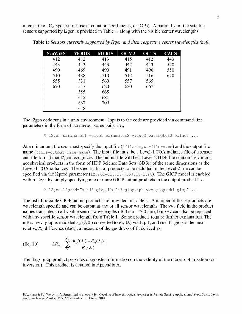
interest (e.g., Ca, spectral diffuse attenuation coefficients, or IOPs). A partial list of the satellite sensors supported by l2gen is provided in Table 1, along with the visible center wavelengths.

Table 1: Sensors currently supported by l2gen and their respective center wavelengths (nm).

SeaWiFS MODIS MERIS OCM2 OCTS CZCS 412 412 413 415 412 443 443 443 443 442 443 520 490 469 490 491 490 550 510 488 510 512 516 670 555 531 560 557 565 670 547 620 620 667

555 665 645 681 667 709 678

The l2gen code runs in a unix environment. Inputs to the code are provided via command-line parameters in the form of parameter=value pairs. i.e.,

% l2gen parameter1=value1 parameter2=value2 parameter3=value3 ...

At a minumum, the user must specify the input file (ifile=input-file-name) and the output file name (ofile=output-file-name). The input file must be a Level-1 TOA radiance file of a sensor and file format that l2gen recognizes. The output file will be a Level-2 HDF file containing various geophysical products in the form of HDF Science Data Sets (SDSs) of the same dimensions as the Level-1 TOA radiances. The specific list of products to be included in the Level-2 file can be specified via the l2prod parameter (l2prod=output-product-list). The GIOP model is enabled within l2gen by simply specifying one or more GIOP output products in the output product list.

% l2gen l2prod=”a_443_giop,bb_443_giop,aph_vvv_giop,chl_giop” ... The list of possible GIOP output products are provided in Table 2. A number of these products are wavelength specific and can be output at any or all sensor wavelengths. The vvv field in the product names translates to all visible sensor wavelengths (400 nm – 700 nm), but vvv can also be replaced with any specific sensor wavelength from Table 1. Some products require further explanation. The mRrs_vvv_giop is modeled rrs’(λ,0-) converted to Rrs’(λ) via Eq. 1, and rrsdiff_giop is the mean relative Rrs difference (ΔRrs), a measure of the goodness of fit derived as:

(Eq. 10)

€

ΔRrs =|Rrs '(λl ) − Rrs(λl ) |

Rrs(λl )l=1

Nw

∑

The flags_giop product provides diagnostic information on the validity of the model optimization (or inversion). This product is detailed in Appendix A.


6

Table 2: GIOP products that can be output by l2gen.

Product Name Description a_vvv_giop total absorption coefficient (m-1) aph_vvv_giop absorption of phytoplankton (m-1) adg_vvv_giop absorption of gelbstof and detritus (m-1) bb_vvv_giop total backscattering (m-1) bbp_vvv_giop backscattering of particles (m-1) chl_giop chlorophyll concentration (mg m-3) adgs_giop Sdg spectral parameter for adg, specified or derived bbps_giop Sbp spectral parameter for bbp, specified or derived mRrs_vvv_giop Rrs’ as reconstructed from the model (sr-1) rrsdiff_giop relative difference between input Rrs and modeled Rrs’ iter_giop number of iterations to achieve convergence flags_giop algorithm performance flags

As currently configured, the default settings for the GIOP model are such that it will reproduce the popular Garver-Siegel-Maritorena model (GSM, Maritorena et al. 2002). In the future, the default settings for GIOP will reproduce the model configuration that is selected for operational IOP product generation within the OBPG. The GIOP model components and optimization method can be modified, however, through the use of various command-line parameters. The available configuration options for GIOP are explained in the sequence of subsections that follow. Option 1: selection of eigenvector(s) for

€

aΦ*(λ)

By default, the GIOP model uses a single, fixed

€

aΦ*(λ) taken from the GSM model and provided to

the program through an external file of tabulated values. The user can specify an alternate file of tabulated values (ascii text, comma or space-delimited), wherein the first column is a list of wavelengths and the 2nd through

€

NΦ +1 column are the associated

€

aΦ*(λ) values. The number of

columns determines the number of eigenvectors to be included in the model. Alternatively, the user can specify the Ca-dependent spectrum of Bricaud et al. (1995) or the size-fraction-dependent spectrum of Ciotti et al. (2002), where the latter requires the additional specification of the desired size fraction. The command-line options for

€

aΦ*(λ) are listed below.

giop_aph_opt = model aph function type 0: tabulated (supplied via giop_aph_file) 2: Bricaud et al 1995 (chlorophyll supplied via empirical algorithm) 3: Ciotti et al. 2002 (size fraction supplied via giop_aph_s) giop_aph_file = tabulated aph spectra giop_aph_s = spectral parameter for aph


7

Option 2: selection of eigenvector(s) for

€

adg*(λ)


€

adg*(λ) taken from the GSM model and provided to

the program through an external file of tabulated values. The default file is actually just an exponential with fixed exponent Sdg=0.02061 (Eq. 6). The user may specify an alternate file of tabulated values, or request to use an exponential function with a fixed or dynamically determined exponent. Dynamically-determined options include the method from the Lee et al. (2002) and an as yet unpublished method developed by Werdell where: (Eq. 11)

€

Sdg = 0.015 + 0.0038 log10[Rrs(443) /Rrs(555)] The command-line options for

€

adg*(λ) are listed below.

giop_adg_opt = adg function type 0: tabulated (supplied via giop_adg_file) 1: exponential with exponent supplied via giop_adg_s 2: exponential with exponent derived via Lee et al. (2002) method 3: exponential with exponent derived via OBPG method giop_adg_file = tabulated adg spectra giop_adg_s = spectral parameter for adg Option 3: selection of eigenvector(s) for

€

bbp*(λ)


€

bbp*(λ) taken from the GSM model and provided to

the program through an external file of tabulated values. The default file contains a power-law with fixed exponent Sbp=1.03373 (Eq. 7). The user may specify an alternate file of tabulated values, or request to use a power-law function with a fixed or dynamically determined exponent. Numerous methods for determination of Sbp are listed among the command-line options for

€

bbp*(λ) below. Loisel

and Stramski (2000) is a unique approach wherein total

€

bbp (λ) is independently derived at each wavelength (no smooth function is assumed). Option 7 below uses Sbp as retrieved from the Loisel & Stramski (2000) model by fitting a powerlaw to the retrieved

€

bbp (λ) , while option 8 treats

€

bbp (λ) itself as the eigenvector (i.e., GIOP uses the shape from Loisel and Stramski but allows the magnitude to vary). The GIOP model also allows for the possibility of fixing

€

bbp (λ) in the absolute sense, and thus solving only for the eigenvalues associated with total a(λ). In this case, the fixed

€

bbp (λ) can come from either Loisel and Stramski (2000) or Lee et al (2002), where the latter provides an algebraic solution for determining

€

bb (λ) and thus

€

bbp (λ) .


8

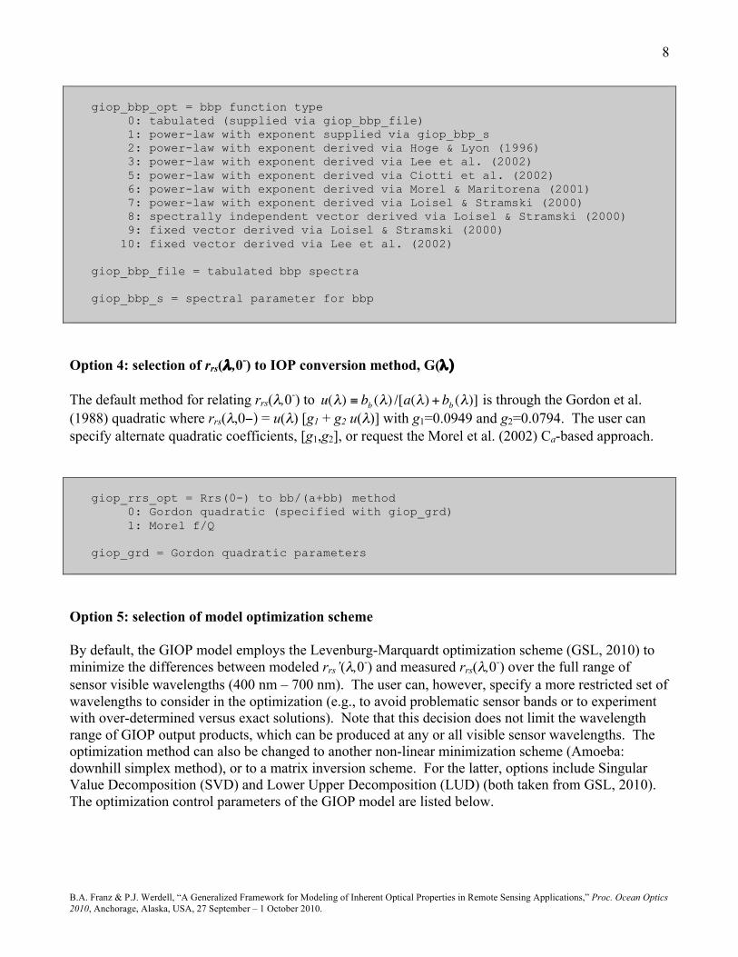
giop_bbp_opt = bbp function type 0: tabulated (supplied via giop_bbp_file) 1: power-law with exponent supplied via giop_bbp_s 2: power-law with exponent derived via Hoge & Lyon (1996) 3: power-law with exponent derived via Lee et al. (2002) 5: power-law with exponent derived via Ciotti et al. (2002) 6: power-law with exponent derived via Morel & Maritorena (2001) 7: power-law with exponent derived via Loisel & Stramski (2000) 8: spectrally independent vector derived via Loisel & Stramski (2000) 9: fixed vector derived via Loisel & Stramski (2000) 10: fixed vector derived via Lee et al. (2002) giop_bbp_file = tabulated bbp spectra giop_bbp_s = spectral parameter for bbp

Option 4: selection of rrs(λ ,0-) to IOP conversion method, G(λ) The default method for relating rrs(λ,0-) to

€

u(λ) ≡ bb (λ) /[a(λ) + bb (λ)] is through the Gordon et al. (1988) quadratic where rrs(λ,0−) = u(λ) [g1 + g2 u(λ)] with g1=0.0949 and g2=0.0794. The user can specify alternate quadratic coefficients, [g1,g2], or request the Morel et al. (2002) Ca-based approach. giop_rrs_opt = Rrs(0-) to bb/(a+bb) method 0: Gordon quadratic (specified with giop_grd) 1: Morel f/Q giop_grd = Gordon quadratic parameters Option 5: selection of model optimization scheme By default, the GIOP model employs the Levenburg-Marquardt optimization scheme (GSL, 2010) to minimize the differences between modeled rrs’(λ,0-) and measured rrs(λ,0-) over the full range of sensor visible wavelengths (400 nm – 700 nm). The user can, however, specify a more restricted set of wavelengths to consider in the optimization (e.g., to avoid problematic sensor bands or to experiment with over-determined versus exact solutions). Note that this decision does not limit the wavelength range of GIOP output products, which can be produced at any or all visible sensor wavelengths. The optimization method can also be changed to another non-linear minimization scheme (Amoeba: downhill simplex method), or to a matrix inversion scheme. For the latter, options include Singular Value Decomposition (SVD) and Lower Upper Decomposition (LUD) (both taken from GSL, 2010). The optimization control parameters of the GIOP model are listed below.


9

giop_wave = list of sensor wavelengths for optimization giop_fit_opt = model optimization method 0: Amoeba optimization 1: Levenberg-Marquardt optimization 2: LUD matrix inversion 3: SVD matrix inversion giop_maxiter = model iteration limit Software Access The GIOP modeling code of l2gen is freely distributed with the SeaWiFS Data Analysis System (SeaDAS, Baith et al., 2001). SeaDAS also provides a graphical user interface (GUI) to simplify manipulation of the many options. Users should be aware, however, that the GIOP code is in active development and the option list is subject to change. The current set of options can always be obtained by simply running l2gen from the unix command-line with no arguments. SUMMARY A generalized framework for developing and testing IOP models was developed and is now available for research. The GIOP model incorporates many ideas from previously published bio-optical models and methods. Through this mechanism, the researcher has the ability to isolate and evaluate individual differences between models in a controlled environment (i.e., all else being equal). Other applications include parametric sensitivity studies and regional tuning of common model forms (e.g., Magnuson et al., 2004). The GIOP framework is also a powerful tool for constructing and evaluating new models through unique combinations of eigenvectors and inversion methods. With power, however, comes responsibility. Models can be constructed with a level of complexity that simply cannot be resolved from the spectral information available. If the specified eigenvectors are not spectrally unique, for example, the optimization of the eigenvalues will be highly correlated, uncertainties will be large, and the problem may not converge. The information contained in the measured Rrs(λ) is also generally correlated between wavelengths, so adding spectral bands does not necessarily provide more information or better constrain the solution. It is the responsibility of the user to recognize these limitations and form the problem accordingly. Caveat emptor. The OBPG developed the GIOP modeling framework to support the activities of the IOP working group (Werdell, 2009), wherein we hope to develop community consensus on an algorithm for producing global IOP products from SeaWiFS, MODIS, and MERIS. This is a work in progress, and many of the options incorporated into the GIOP model were developed in collaboration with the IOP working group. Future plans include the addition of temperature and salinity effects on aw(λ) and bbw(λ), support for alternative approaches to determine G(λ) (e.g., Smyth et al., 2006), and incorporation of a generalized scheme for producing uncertainties on the derived IOP products (e.g., Wang et al., 1995; Lee et al., 2010; Maritorena et al., 2010).


10

REFERENCES Baith, K., R. Lindsay, G. Fu, and C.R. McClain (2001). Data analysis system developed for ocean color satellite sensors. EOS Transactions AGU, 82, 202. http://oceancolor.gsfc.nasa.gov/seadas/. Boss, E.S., and S. Maritorena (2006). Uncertainties in the products of ocean-colour remote sensing, in Remote Sensing of Inherent Optical Properties: Fundamentals, Tests of Algorithms and Applications, Z.-P. Lee, ed. (IOCCG, 2006). Boss, E.S., and C. Roesler (2006). Over Constrained Linear Matrix Inversion with Statistical Selection, in Remote Sensing of Inherent Optical Properties: Fundamentals, Tests of Algorithms and Applications, Z.-P. Lee, ed. (IOCCG, 2006). Bricaud, A., M. Babin, A. Morel, and H. Claustre (1995). Variability in the chlorophyll-specific absorption coefficients of natural phytoplankton: analysis and parameterization, J. Geophys. Res., (100) 13321–13332. Ciotti, A.M., Lewis, M.R., and Cullen, J.J. (2002). Assessment of the relationships between domininant cell size in natural phytoplankton communities and spectral shape of the absorption coefficient. Limnol. Oceanogr., 47, 404- 417. Franz, B.A. (2010). l2gen: The Multi-Sensor Level-1 to Level-2 Generator, Ocean Color Web, http://oceancolor.gsfc.nasa.gov/WIKI/OCSSW(2f)l2gen.html. GSL (2010), “GNU Statistics Library”, http://www.gnu.org/software/gsl/manual/html_node/. IOCCG (2006). Remote Sensing of Inherent Optical Properties: Fundamentals, Tests of Algorithms, and Applications. Edited by ZhongPing Lee, pp. 126. Garver, S.A., and Siegel, D. (1997). Inherent optical property inversion of ocean color spectra and its biogeochemical interpretation 1. Time series from the Sargasso Sea, J. Geophys. Res. (102) 18607-18625. Hoge, F.E., and P.E. Lyon (1996). Satellite retrieval of inherent optical properties by linear matrix inversion of oceanic radiance models: an analysis of model and radiance measurement errors. J. Geophys. Res. (101) 16631-16648. Lee, Z.P., Carder, K.L., and Arnone, R. (2002). Deriving inherent optical properties from water color: A multi-band quasi-analytical algorithm for optically deep waters. Appl. Opt. (41) 5755-5772. Lee, Z.-P., R. Arnone, C. Hu, P.J. Werdell, and B. Lubac (2010). Uncertainties of optical parameters and their propagations in an analytical ocean color inversion algorithm, Appl. Opt. (49) 369-381. Loisel, H., and Stramski, D. (2000). Estimation of the inherent optical properties of natural waters from the irradiance attenuation coefficient and reflectance in the presence of Raman scattering. Appl. Opt. (39) 3001-3011.


11

Magnuson, A., L.W. Harding Jr., M.E. Mallonee and J.E. Adolf (2004). Bio-optical model for Chesapeake Bay and the middle Atlantic bight. Estuar. Coast. Shelf Sci. (61) 403-424. Maritorena S., D.A. Siegel and A. Peterson (2002). Optimization of a Semi-Analytical Ocean Color Model for Global Scale Applications. Applied Optics, 41(15) 2705-2714. Maritorena, S., O.H.F. d’Andon, A. mangin, D.A. Siegel (2010). Merged satellite ocean color data products using a bio-optical model: Characteristics, benefits and issues, Rem. Sens. Env. (114) 1791-1804. Morel, A. and L. Prieur (1977). Analysis of variations in ocean color, Limnol. Oceanogr. (22) 709. Morel, A., and S. Maritorena (2001). Bio-optical properties of oceanic waters: A reappraisal, J. Geophys. Res., 106, 7763-7780. Morel, A., D. Antoine and B. Gentili (2002). Bidirectional Reflectance of Oceanic Waters: Accounting for Raman Emission and Varying Particle Scattering Phase Function, Appl. Opt. (41) 6289-6306. O’Reilly, J.E., Maritorena, S., Mitchell, B.G., Siegel, D.A., Carder, K.L., Garver, S.A., Kahru, M., and McClain, C. (1998), Ocean color chlorophyll algorithms for SeaWiFS. J. Geophys. Res., 103, 24937-24953. Pope, R.M. and E. S. Fry (1997). Absorption spectrum (380–700 nm) of pure water. II. Integrating cavity measurements, Appl. Opt. (36) 8710–8723. Prieur, L., and S. Sathyendranath (1981). An optical classification of coastal and oceanic waters based on the specific spectral absorption curves of phytoplankton pigments, dissolved organic matter, and other particulate materials, Limnol. Oceanogr., 26(4), 671-689. Roesler, C.S., and Perry, M.J. (1995). In situ phytoplankton absorption, fluores- cence emission, and particulate backscattering spectra determined from reflectance. J. Geophys. Res. 100: 13279-13294. Smith, R.C. and Karen S. Baker (1981). Optical properties of the clearest natural waters (200–800 nm), Appl. Opt., (20) 177-184. Smyth, T.J., G.F. Moore, T. Hirata, and J. Aiken (2006). Semianalytical model for the derivation of ocean color inherent optical properties: description, implementation, and performance assessment. Appl. Opt., 45: (31) 8116-8131. Wang, P., E.S. Boss, and C. Roesler (2005). Uncertainties of inherent optical properties obtained from semianalytical inversions of ocean color, Appl. Opt., 44, 4074-4085. Werdell, P.J. (2009). Global bio-optical algorithms for ocean color satellite applications, EOS Trans. AGU (Meeting Report) 90, 4 (2009). http://oceancolor.gsfc.nasa.gov/MEETINGS/OOXIX/IOP/.


12

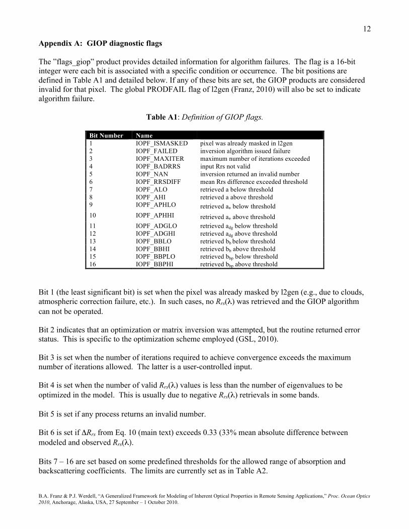
Appendix A: GIOP diagnostic flags The ”flags_giop” product provides detailed information for algorithm failures. The flag is a 16-bit integer were each bit is associated with a specific condition or occurrence. The bit positions are defined in Table A1 and detailed below. If any of these bits are set, the GIOP products are considered invalid for that pixel. The global PRODFAIL flag of l2gen (Franz, 2010) will also be set to indicate algorithm failure.

Table A1: Definition of GIOP flags.

Bit Number Name 1 IOPF_ISMASKED pixel was already masked in l2gen 2 IOPF_FAILED inversion algorithm issued failure 3 IOPF_MAXITER maximum number of iterations exceeded 4 IOPF_BADRRS input Rrs not valid 5 IOPF_NAN inversion returned an invalid number 6 IOPF_RRSDIFF mean Rrs difference exceeded threshold 7 IOPF_ALO retrieved a below threshold 8 IOPF_AHI retrieved a above threshold 9 IOPF_APHLO retrieved aΦ below threshold 10 IOPF_APHHI retrieved aΦ above threshold 11 IOPF_ADGLO retrieved adg below threshold 12 IOPF_ADGHI retrieved adg above threshold 13 IOPF_BBLO retrieved bb below threshold 14 IOPF_BBHI retrieved bb above threshold 15 IOPF_BBPLO retrieved bbp below threshold 16 IOPF_BBPHI retrieved bbp above threshold

Bit 1 (the least significant bit) is set when the pixel was already masked by l2gen (e.g., due to clouds, atmospheric correction failure, etc.). In such cases, no Rrs(λ) was retrieved and the GIOP algorithm can not be operated. Bit 2 indicates that an optimization or matrix inversion was attempted, but the routine returned error status. This is specific to the optimization scheme employed (GSL, 2010). Bit 3 is set when the number of iterations required to achieve convergence exceeds the maximum number of iterations allowed. The latter is a user-controlled input. Bit 4 is set when the number of valid Rrs(λ) values is less than the number of eigenvalues to be optimized in the model. This is usually due to negative Rrs(λ) retrievals in some bands. Bit 5 is set if any process returns an invalid number. Bit 6 is set if ΔRrs from Eq. 10 (main text) exceeds 0.33 (33% mean absolute difference between modeled and observed Rrs(λ). Bits 7 – 16 are set based on some predefined thresholds for the allowed range of absorption and backscattering coefficients. The limits are currently set as in Table A2.


13

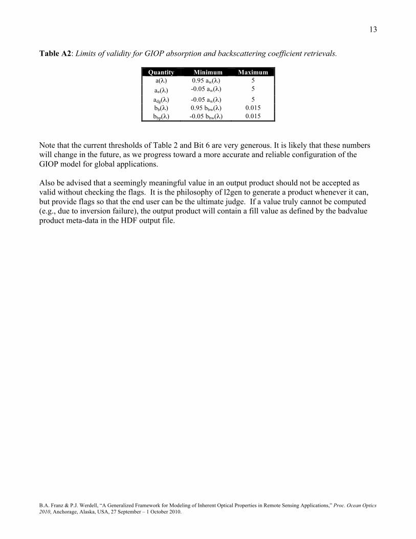
Table A2: Limits of validity for GIOP absorption and backscattering coefficient retrievals.

Quantity Minimum Maximum a(λ) 0.95 aw(λ) 5 aΦ(λ) -0.05 aw(λ) 5 adg(λ) -0.05 aw(λ) 5 bb(λ) 0.95 bbw(λ) 0.015 bbp(λ) -0.05 bbw(λ) 0.015

Note that the current thresholds of Table 2 and Bit 6 are very generous. It is likely that these numbers will change in the future, as we progress toward a more accurate and reliable configuration of the GIOP model for global applications. Also be advised that a seemingly meaningful value in an output product should not be accepted as valid without checking the flags. It is the philosophy of l2gen to generate a product whenever it can, but provide flags so that the end user can be the ultimate judge. If a value truly cannot be computed (e.g., due to inversion failure), the output product will contain a fill value as defined by the badvalue product meta-data in the HDF output file.

A Generalized Framework for Modeling of Inherent Optical ... · B.A. Franz & P.J. Werdell, “A...

Documents

Transcript of A Generalized Framework for Modeling of Inherent Optical ... · B.A. Franz & P.J. Werdell, “A...