A GENERALIZATION OF BARABÁSI PRIORITY MODEL … · A GENERALIZATION OF BARABÁSI PRIORITY MODEL OF...

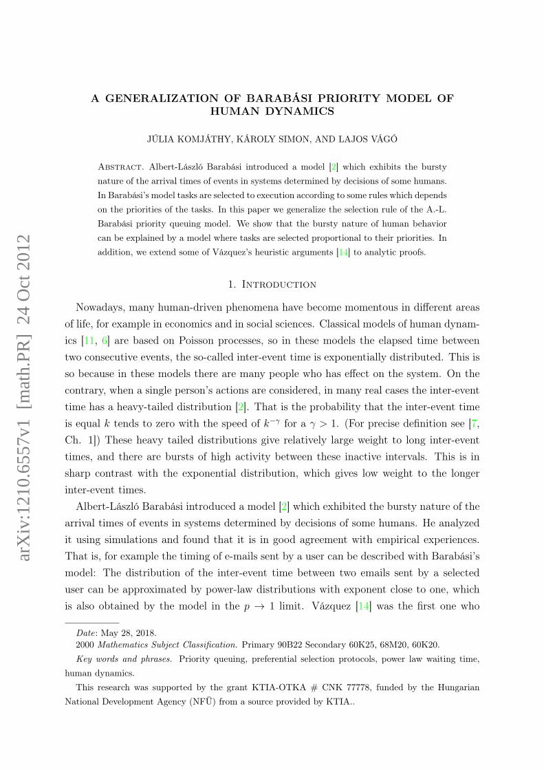
A GENERALIZATION OF BARABÁSI PRIORITY MODEL OFHUMAN DYNAMICS

JÚLIA KOMJÁTHY, KÁROLY SIMON, AND LAJOS VÁGÓ

Abstract. Albert-László Barabási introduced a model [2] which exhibits the burstynature of the arrival times of events in systems determined by decisions of some humans.In Barabási’s model tasks are selected to execution according to some rules which dependson the priorities of the tasks. In this paper we generalize the selection rule of the A.-L.Barabási priority queuing model. We show that the bursty nature of human behaviorcan be explained by a model where tasks are selected proportional to their priorities. Inaddition, we extend some of Vázquez’s heuristic arguments [14] to analytic proofs.

1. Introduction

Nowadays, many human-driven phenomena have become momentous in different areasof life, for example in economics and in social sciences. Classical models of human dynam-ics [11, 6] are based on Poisson processes, so in these models the elapsed time betweentwo consecutive events, the so-called inter-event time is exponentially distributed. This isso because in these models there are many people who has effect on the system. On thecontrary, when a single person’s actions are considered, in many real cases the inter-eventtime has a heavy-tailed distribution [2]. That is the probability that the inter-event timeis equal k tends to zero with the speed of k−γ for a γ > 1. (For precise definition see [7,Ch. 1]) These heavy tailed distributions give relatively large weight to long inter-eventtimes, and there are bursts of high activity between these inactive intervals. This is insharp contrast with the exponential distribution, which gives low weight to the longerinter-event times.

Albert-László Barabási introduced a model [2] which exhibited the bursty nature of thearrival times of events in systems determined by decisions of some humans. He analyzedit using simulations and found that it is in good agreement with empirical experiences.That is, for example the timing of e-mails sent by a user can be described with Barabási’smodel: The distribution of the inter-event time between two emails sent by a selecteduser can be approximated by power-law distributions with exponent close to one, whichis also obtained by the model in the p → 1 limit. Vázquez [14] was the first one who

Date: May 28, 2018.2000 Mathematics Subject Classification. Primary 90B22 Secondary 60K25, 68M20, 60K20.Key words and phrases. Priority queuing, preferential selection protocols, power law waiting time,

human dynamics.This research was supported by the grant KTIA-OTKA # CNK 77778, funded by the Hungarian

National Development Agency (NFÜ) from a source provided by KTIA..

arX

iv:1

210.

6557

v1 [

mat

h.PR

] 2

4 O

ct 2

012

2 JÚLIA KOMJÁTHY, KÁROLY SIMON, AND LAJOS VÁGÓ

studied the model analytically. He confirmed Barabási’s results by determining the exactdistribution of the priorities and the waiting time at stationarity. He found that in thep→ 1 limit the distribution of the waiting time is close to a power-law distribution withexponent one.

In this paper, motivated by the work of Barabási [2] and Vázquez [14], we generalizethis model to a more general one, where burstiness occurs as well. This generalizationshows that this power-law decay with exponent 1 can be obtained in sequences of modelswhere tasks with higher priority are more and more likely to be chosen. In addition, weextend some of Vázquez’s heuristic arguments to analytic proofs.Barabási’s model is as follows: Somebody has a todo list which always consists of

exactly L items, each of which has a non-negative priority. In every discrete time step(1, 2, . . . ) two things happen:

• A task is selected for execution according to a selection protocol described laterand leaves the system,• another task arrives to the list.

The priority of all arriving task including the tasks at the 0-th step are i.i.d. randomvariables with an absolutely continuous distribution function R(x) on [0,∞). Let us calla task new at time t if it has just arrived to the list. We denote by Nt the priority of thenew task and let us introduce

R(x) := P(Nt ≤ x).

The corresponding density function (DF) is

r(x) := R′(x).

Throughout the paper we assume that

r ∈ L2(0, 1).

In addition, let us call a task old at time t, if it was on the list at time t − 1 at it isstill there at time t. We denote its priority by Ot and denote its cumulative distributionfunction by

R1(x, t) := P(Ot ≤ x),

and its density

r1(x, t) :=d

dxR1(x, t).

The selection protocol in Barabási’s model is as follows: Independently in each stepindependently, we toss a coin with probability of heads 0 ≤ p ≤ 1. If heads, the task withthe highest priority is selected for execution and leaves the system. If tails, a task selecteduniformly from the list leaves the system. In particular, if p = 1, then we use the highestpriority first selection protocol, and if p = 0, then the selection is completely uniform. Letus denote by τ the waiting time of a task to for execution, that is, the number of steps

A GENERALIZATION OF BARABÁSI PRIORITY MODEL OF HUMAN DYNAMICS 3

between its arrival at and its departure from the system. Using computer simulations,Barabási found that if p→ 1 then the waiting time τ has a power law tail with exponent1 . These asymptotics hold not only for long lists but even if the list consists of two items,that is for L = 2. In this case Vázquez [14] proved analytically that

(1.1) limp→1

P(τ = k) =

1 +O(

1−p2

ln(1− p))

if k = 1,

O(

1−p2

)1

k−1if k > 1.

In [14] the expected value of the waiting time was also investigated. For the case L = 2

Vázquez proved analytically that

E(τ) =

2, if p<1;1, p=1

in stationarity. If p = 1 this means that there is a task stuck in the queue with priority0. For the case L > 2 Vázquez conjectured that

Conjecture 1.1 (Vázquez).

E(τ) =

L, if p<1;1, p=1

in stationarity. If p = 1 stationarity means that there are L− 1 tasks stuck.

Our work is divided into two main parts.

1.1. Barabási model. We extend some of the heuristic arguments of [14] related to theBarabási model to analytic proofs in Section 3. We distinguish two cases according top < 1 or p = 1.

1.1.1. Barabási model with p < 1. First we assume that 0 ≤ p < 1. We extend Vázquez’scompletely correct heuristic argument to an analytic proof in Section 3.1.

1.1.2. Barabási model with p = 1. Then in Section 3.2 we consider the case when at everytime step the task with the highest priority is selected. Although the relevant part ofVázquez’s Conjecture 1.1 holds but the stationary case will not be achieved, since therewill never be any tasks with priority 0 almost surely. It is of crucial importance to observethat in this case at time t the L items on the list are as follows: Beside the newly addeditem we have the L − 1 lowest priority items among all items which have ever added tothe list. Therefore we can use the theory of the process of records. We study this case forL = 2 in Section 3.2, where all tasks remain on the list for one time step except for therecords. An item is called lower record (from which we usually omit to say the adjectivelower) if it has the lowest priority at the time when it is added to the list. When sucha record arrives, then it remains on the list until a new record arrives. The time elapsedbetween the n-th and n+ 1-th records called the n-th inter-record time. It is well knownthat the expected value of the inter-record times grow exponentially with n. Therefore


simulations may indicate the false conclusion that one task remains indefinitely in thequeue [14] [2].

1.2. Generalization of the Barabási model. In Section 4 We study the Barabási-model for general priority-based selection protocols in the case L = 2. We analyze thetwo main characteristics of this model at stationarity, namely the distribution of thepriorities of tasks on the list and that of τ , the waiting time a task spends on the listbefore execution. To explain these with more detail, we need to introduce some newnotation. At time t + 1 there are two items on the list. The one which has just arrivedto the list we call new, and the one which was already on the list at time t we call it oldtask. The distribution of the new task is given by R(x). Our goal is to understand thedistribution of the old task. The selection protocol is described by the function v in thefollowing way:

v(x, y) := P(new is chosen | new has priority x, old has priority y),

where ∀y v(., y) is increasing and ∀x v(x, .) is decreasing. Furthermore we assume that∀x ∀y v(x, y) ≤ c1 < 1 with some constant c1.

We use Vázquez’s notation, and also refer to the results in [14] for the Barabási case,when v(x, y) = p1x>y + 1−p

2(the model introduced by Barabási [2]). An other natural

example is as follows.

Example 1.2. Let v be v(x, y) = p xx+y

+ 1−p2, 0 ≤ p ≤ 1 and the priority of the new task

is uniformly distributed on [c, 1], 0 < c < 1. That is, first we toss a biased coin (headswith probability p). If heads, we select a task for execution proportionally to the priorities,if tails, the selection is done uniformly. This model takes into account not only the orderof priorities, but also the proportion of those.

If tasks are interpreted as being competitors and the priorities as levels of talent of thesecompetitors, then Example 1.2 can be explained as follows: In a game, every competitorentering the game have to play until he wins for the first time. We also know that theoutcome of the games depends on the level of talents as it is determined by the selectionprotocol of Example 1.2. That is, with probability p the chances to win are proportionalto the level of talents of the two competitors, and with probability 1− p the competitorswin with 1

2-1

2probability. The a priori distribution of the talent of a player is uniform on

[c, 1], and the game has been going on for a long time. We are interested in the distributionof the level of talent of a player about whom we only know that he has just lost a game.Then the corresponding density function r1(x) is illustrated in Section 4.2, see Fig. 2.

Very useful notations are the following ones. The probability that the new task isselected given the old task has priority s is

(1.2) q(s) =

∫ 1

0

v(y, s)dR(y),


and the probability that the new task is selected given the old task has priority s is

q1(s, t) =

∫ 1

0

(1− v(s, y))dR1(y, t).

With these notations one can easily describe the evolution of R(x, t). Assume that attime t+ 1 the old task is T ∗. Then either

(a) T ∗ was the old task at time t, or(b) T ∗ was the new task at time t.

In the first case (a), the new task had to be selected for execution in step t, so that T ∗

remained in the system, and in the other case (b) the old task had to be selected so thatT ∗ remained in the system. Hence law of total probability gives us

R1(x, t+ 1) =

∫ x

0

r1(s, t)q(s)ds︸︷︷︸case(a)

+

∫ x

0

r(s)q1(s, t)ds︸︷︷︸case(b)

.

Assuming the system is in stationary state, the probability that the old task is selectedgiven the new task has priority s is

(1.3) q1(s) =

∫ 1

0

(1− v(s, y))dR1(y),

and for the stationary CDF R1(x) and DF r1(x) of the priority of the old task we obtainthe stationary equation

(1.4) R1(x) =

∫ x

0

r1(s)q(s)ds+

∫ x

0

r(s)q1(s)ds.

In the very special Barabási case R1(x) can be explicitly computed [14]. However, in thegeneral case the function R1(x) cannot be expressed by a closed formula. We will useHilbert- Schmidt operator techniques to find an approximation of R1(x).

As far as the waiting time is concerned, the distribution of τ is:

(1.5) P(τ = k) =

∫ 1

0(1− q1(x))dR(x) if k = 1,∫ 1

0q1(x)(1− q(x))q(x)k−2dR(x) if k > 1.

If k = 1, then the task has to be executed immediately, so the probability of this is exactly1− q1(x) if the task has priority x. Otherwise, if k > 1, then the event that a task withpriority x stays exactly k steps on the waiting list is the intersection of k conditionallyindependent events. When the task is added to the list, it must not be executed, thishappens with probability q1(x), then it becomes old and has to stay k − 2 more steps onthe list, the probability of this event is q(x)k−2, and finally, the task has to be executed,which event has probability 1− q(x).

In the Barabási case these integrals can be explicitly computed [14], hence we obtain

P(τ = k) =

1− 1−p24pln1+p

1−p if k = 1,1−p2

4p

((1+p

2

)k−1 −(

1−p2

)k−1)

1k−1

if k > 1.


In the limit p→ 1 it leads to (1.1).In the general case only the expected waiting time can be explicitly computed, see

Section 3.1.

2. Probabilistic interpretation of R1(x) in the Barabási case

Consider the Barabási case with p < 1. As we mentioned earlier, Vázquez [14] computedR1(x) in the Barabási case. In order to give a better understanding of the nature of themodel, here we provide an alternative, probabilistic way to compute the CDF R1(x). Partof this method will be used when we prove Conjecture 1.1.

To get the distribution function R1(x) of the old task in a stationary system, firstextend the dynamics backwards in time such that the values of the system at −1,−2, . . .

are defined to maintain stationarity. Further, let us suppose that the process is stationaryat time T . Starting from this T , we are looking backwards in time and count how manyother tasks had an old task to compete with in order to be able to stay in the list untilT . We define the following three events:

• Rnew :=The selection protocol turns out to be the random choice and

a new task is executed.

In this case the new task leaves the list immediately. Thus, the old task does nothave to compete with its priority at all, so we do not have to count these cases.This event happens in each step with probability 1−p

2.

• Rold :=Random protocol is chosen, and the old task is selected.

In this case the arriving new task becomes old and the old task before it leaves thesystem. Since the priority distribution of the new task is just R(x), consideringthe old task’s priority distribution, the system restarts at each event of this type.This event happens in each step with probability 1−p

2.

• Rcomp :=Priority selection.

This third event happens with probability p.

Thus the process can be coded by sequences of type Rnew, Rold, RcompZ.Let Xt be the t-th element of this sequence. Then the renewal at every Rold event can

be formalized as follows: Using the fact that the sequence Xt∞t=1 is independent of thepriorities, for every x ∈ R

P(Ot+1 < x | Xt = Rold) = P(Nt < x | Xt = Rold) = P(Nt < x) = R(x),

where recall that Ot and Nt stands for the priority of the old and the new task at timestep t, respectively.

Since the priority distribution of the old task is renewed at every event Rold, in orderto determine the priority distribution of the old task in the system for a big enough T ,we have to count how many Rcomp-s we had after the last Rold event.


It is easy to see that the distribution of the arrival time of the last Rold event is justT − GEO

(1−p

2

)+ 1. Similarly, if we only want to count the number of Rcomp-s after

the last Rold, we have to re-normalize the probabilities to exclude cases of Rnew, so it’sdistribution is

GEO

(1−p

2

p+ 1−p2

)− 1 = GEO

(1− p1 + p

)− 1.

Thus, the old task in the system at time T had to compete with the other tasks ateach event Rcomp and had to "win", i.e its priority had to be less than all of them, inorder to stay in the system up to time T . So, its priority had to "defeat" GEO

(1−p1+p

)− 1

many other tasks to stay in the list so far. Hence the distribution we were looking foris the minimum of X ∼ GEO

(1−p1+p

)many independent random variables (YiXi=1), of

distribution R(x). Let us compute it’s CDF using the law of total probability:

F (x) = P( mini=1...X

Yi < x) =∞∑k=1

P(∃i ≤ X : Yi ≤ x | X = k)P(X = k)

=1 + p

2

(1− 1

1 + 2p1−pR(x)

),

in agreement with [14], since the summation converges if p < 1. A comment is that weonly used the extension to doubly infinite stationary sequence since the geometric variablein this proof is unbounded.

3. Records and expected waiting time

3.1. Ergodicity for p < 1. In this section we verify Conjecture 1.1 which gives us theexpected waiting time in the Barabási case. Let us first set p < 1 and L ≥ 2. We usethe method suggested by Vázquez [14], and work out the details. Using the argumentsintroduced by Vázquez let us denote by τi the waiting time of the task executed at stepi, and by τ ′l,t (l = 1, . . . , L− 1) the resident times of the tasks that are still in the bufferat step t. Then we summarize the main point in the following theorem:

Theorem 3.1. [Ergodic Theorem for L ≥ 2, p < 1.] The priority queuing system in theBarabási case is ergodic for any L ≥ 2 and p < 1 and the following limit holds:

(3.1) EL(τ) = limt→∞

1

t

t∑i=1

τi = L a.s. and in L1.

Proof. Since the total buffer time until time t is Lt and in each time step exactly one taskleaves the system, we have that

t∑i=1

τi +L−1∑l=1

τ ′l,t = Lt.


Hence

(3.2) limt→∞

1

t

t∑i=1

τi = L− limt→∞

1

t

L−1∑l=1

τ ′l,t

if these limits exist. Similarly to the L = 2 case in Section 2, the process renews wheneverthere are L − 1 successive Rold events, where Rold means that the oldest task is selectedfor execution because of the random selection. For every t the probability that there is arenewal section of the process starting at the step t is

(1−pL

)L−1. In addition, two renewalsections starting at time t1 and t2 are independent if |t1 − t2| ≥ L − 1. So the systemrenews infinitely often a.s.. (This implies also the existence of a stationary distributionfor the L − 1 not newly added task’s priority.) Analogous to the argument in Section 2,each remaining time τ ′l,t can be stochastically dominated by a geometric random variable

with success probability (1−pL

)L−1. Thus,τ ′l,tt→ 0 as t→∞ holds for any l almost surely

(a.s.) and in L1, and so we obtain

(3.3) limt→∞

1

t

L−1∑l=1

τ ′1,t = 0 a.s. and in L1.

There remains the proof of ergodicity. Let us denote by M t = (M1t , . . . ,M

L−1t ) the

L − 1 dimensional vector of the oldest elements in the buffer at time t, such that M1t is

the priority of the oldest, M it is the priority of the i-th oldest task in the system. Then

clearly the sequence M t∞t=1 is Markovian with state space [0, 1]L−1. Moreover, it isclearly aperiodic, and since the system renews infinitely often a.s., it is irreducible. Thusergodicity and equations (3.2) and (3.3) immediately imply (3.1) as it was suggested byVázquez’s heuristic arguments [14].

3.2. Records. In this section we investigate the case p = 1, L = 2 , i.e. the case whenthe selection protocol has no randomness and always picks the task in the system withhigher priority. We show that the system achieves no stationary distribution in this case.

It is easy to see that when a task arrives whose priority is less than all the prioritiesbefore, then the old task in the system will be chosen for execution and this task willremain in the buffer. This implies that R1(x, t) (the distribution of the old task’s priorityat time t) is the distribution of the minimum, i.e. the lower record value of the first t+ 2

tasks’ priority. That is, we need to consider the minimum of t+ 2 i.i.d. random variableswith distribution R(x).

On the other hand, a stationary distribution Rs1(x) should satisfy equation (1.4), which

has only a degenerate solution R1(x) = 0 a.s. if p = 1. Thus, the stationary distributionRs

1(t) will never be achieved, since

P(∀t R1(x, t) 6= 0) = 1.

Hence, the properties of the waiting time τ are related to the process of records.


In order to introduce some classical theorems of record theory (for an introduction see[1, p. 22-28]), we will need some definitions.

Definition 3.2. Let Xt∞t=1 be i.i.d. random variables with absolutely continuous CDFF . Then we define the followings:

(1) The sequence Tk∞k=1 of lower record times is defined by

T1 = 1, and for k > 1

Tk = mint | Xt < XTk−1.

(2) The sequence ∆k∞k=2 of inter-record times is defined by

∆k = Tk − Tk−1.

(3) The sequence It∞t=1 of record indicators is defined by

I1 = 1, and for t > 1

It = 1Xt < minX1, . . . , Xt−1.

(4) The sequence xk∞k=1 of lower record values is defined by

xk = XTk .

If we do not care about the record values, without loss of generality one can assume thatthe distribution of the Xi-s is U [0, 1]. Thus one can easily compute the joint distributionof the It-s. Let n, 1 = t1 < t2 < · · · < tn be arbitrary positive integers. Then

P(It1 = 1, . . . , Itn = 1)

=

∫0<x1<···<xn<1

P(It1 = 1, . . . , Itn = 1 | Xt1=x1 , . . . , Xtn=xn)dx1 . . . dxn

=

∫0<x1<···<xn<1

xt2−11 xt3−t2−1

2 . . . xtn−tn−1−1n dx1 . . . dxn

=1

t1

1

t2. . .

1

tn.

Since the integers n, 1 = t1 < t2 < · · · < tn were arbitrary, and the It-s are discrete randomvariables, it is evident that these random variables are independent, and It ∼ BER

(1t

)is a Bernoulli random variable.

Now consider the ratio ∆k

Tk. The distribution of ∆k

Tkconditioned on the value of Tk−1 can

be determined by Tata’s reasoning [13]:

P(

∆k

Tk> x

∣∣∣ Tk−1 = t

)= P

(∆k

t+ ∆k

> x∣∣∣ Tk−1 = t

)= P

(∆k >

x

1− xt∣∣∣ Tk−1 = t

)= P

(It+1 = 0, . . . , Ibt/(1−x)c = 0

)=

t

bt/(1− x)c.


Since Tk →∞ a.s. as k →∞, hence

limk→∞

P(

∆k

Tk> x

)= 1− x,

so thus ∆k

Tkand Tk−1

Tkare asymptotically U [0, 1].

Now we turn back to the Barabási model in the case p = 1 and L = 2. Equation (3.2)holds also in this situation:

limt→∞

1

t

t∑i=1

τi = 2− limt→∞

τ ′1,tt

if these limits exist. But now, with the help of record theory one can prove that the limiton the right hand side does not exist. On the one hand if we choose t = Tk + 1 then weobtain:

lim inft→∞

τ ′1,tt

= 0 a.s.,

since the sequence of records is infinite a.s. (This is ensured by the continuity of the CDFF ), so thus τ ′1,t = 0 will hold for infinitely many t-s. On the other hand the limsup istaken if t = Tk (we look the subsequence of records):

lim supt→∞

τ ′1,tt

= limk→∞

∆k−1

Tk= lim

k→∞

Tk − Tk−1

Tk

= 1− limk→∞

Tk−1

Tk= 1− Z,

where Tk and ∆k are the k-th record and inter-record times, and Z is a U [0, 1] randomvariable.

Thus, Vázquez’s heuristics does not work in this case. Note that the dynamics is noteven ergodic, since the irreducibility does not hold, as the priority of the old task decreasesmonotonically.

Further, we can state precise asymptotic results about the waiting time of the recordsin the queue. It was proven by Holmes and Strawderman [8] that the Strong Law ofLarge Numbers (SLLN), by Neuts [10] that the Central Limit Theorem (CLT) and byStrawderman and Holmes [12] that the Law of Iterated Logarithm (LIL) hold for theseries of lnTk and ln ∆k as well:

Theorem 3.3. Let zk be either ∆k or Tk. Then

(1) [SLLN][8]ln zkk

a.s.→ 1 as k →∞.

(2) [CLT][10]ln zk − k√

k⇒ N(0, 1) as k →∞.


(3) [LIL][12]

lim supk→∞

ln zk − k√2k ln ln k

= 1 a.s.,

lim infk→∞

ln zk − k√2k ln ln k

= −1 a.s. .

Thus we see that the k-th record spends roughly ek time in the buffer.

4. A natural generalization of the model

In this section we consider a common generalization of Barabási’s model and Example1.2 which were not analyzed in the literature before. Also in this new model there is alist with L tasks, the new tasks has i.i.d. non-negative priorities, and in each discretetime step one task is selected to execution and a new task arrives to it’s place. The onlychange is that the dynamics of the system is now given by a general selection protocol.We will analyze this new model for the case L = 2, so we define the selection protocol tothis case. In every time step we select a task according to the priorities in the followingway:

(4.1) v(x, y) := P(new is chosen | new has priority x, old has priority y),

where

Assumption 4.1. We assume that ∀y v(., y) is increasing and ∀x v(x, .) is decreasing.Furthermore let us suppose that

∀x ∀y v(x, y) ≤ c1 < 1

with some constant c1.

Let Ot be the priorities of the old task at time t. Clearly, the sequence Ot∞t=1 is anaperiodic Markov-chain on the state space (0, 1).

Lemma 4.2. Under Assumption 4.1, the Markov-chain Ot∞t=1 defined above is positiverecurrent.

First note that positive recurrence of the Markov chain implies the existence of a station-ary distribution as well. We remind the reader that q(s) and q1(s) was defined in (1.2) and(1.3), and r(x) is the density function of the new task. Since ∃c1 ∀x ∀y v(x, y) ≤ c1 < 1,hence ∀s q(s) =

∫ 1

0v(y, s)dR(y) ≤ c1 < 1 and ∀s q1(s) ≥ 1− c1 > 0.

Proof. For any x ∈ supp(r) let us denote by Tx,y,ε the hitting time from x to (y− ε, y+ ε).Thus the distribution of Tx,y,ε is stochastically dominated by the geometric distributionwith success probability (1− c1)(R(y + ε)−R(y − ε)). Therefore

E(Tx,y,ε) ≤1

(1− c1)(R(y + ε)−R(y − ε))<∞.


Since the Markov chain is ergodic, this fact implies that Theorem 3.1 is valid in thiscase, and the expected waiting time of a task equals 2.

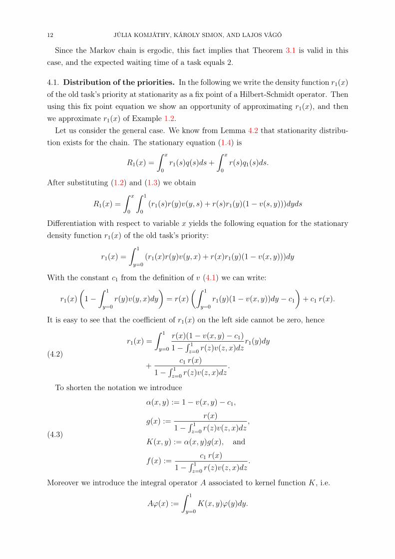
4.1. Distribution of the priorities. In the following we write the density function r1(x)

of the old task’s priority at stationarity as a fix point of a Hilbert-Schmidt operator. Thenusing this fix point equation we show an opportunity of approximating r1(x), and thenwe approximate r1(x) of Example 1.2.

Let us consider the general case. We know from Lemma 4.2 that stationarity distribu-tion exists for the chain. The stationary equation (1.4) is

R1(x) =

∫ x

0

r1(s)q(s)ds+

∫ x

0

r(s)q1(s)ds.

After substituting (1.2) and (1.3) we obtain

R1(x) =

∫ x

0

∫ 1

0

(r1(s)r(y)v(y, s) + r(s)r1(y)(1− v(s, y)))dyds

Differentiation with respect to variable x yields the following equation for the stationarydensity function r1(x) of the old task’s priority:

r1(x) =

∫ 1

y=0

(r1(x)r(y)v(y, x) + r(x)r1(y)(1− v(x, y)))dy

With the constant c1 from the definition of v (4.1) we can write:

r1(x)

(1−

∫ 1

y=0

r(y)v(y, x)dy

)= r(x)

(∫ 1

y=0

r1(y)(1− v(x, y))dy − c1

)+ c1 r(x).

It is easy to see that the coefficient of r1(x) on the left side cannot be zero, hence

(4.2)

r1(x) =

∫ 1

y=0

r(x)(1− v(x, y)− c1)

1−∫ 1

z=0r(z)v(z, x)dz

r1(y)dy

+c1 r(x)

1−∫ 1

z=0r(z)v(z, x)dz

.

To shorten the notation we introduce

(4.3)

α(x, y) := 1− v(x, y)− c1,

g(x) :=r(x)

1−∫ 1

z=0r(z)v(z, x)dz

,

K(x, y) := α(x, y)g(x), and

f(x) :=c1 r(x)

1−∫ 1

z=0r(z)v(z, x)dz

.

Moreover we introduce the integral operator A associated to kernel function K, i.e.

Aϕ(x) :=

∫ 1

y=0

K(x, y)ϕ(y)dy.


Since K ∈ L2[0, 1]× [0, 1], hence A maps L2[0, 1] into itself (see [9, Theorem 9.2.1.]). Withthis notation, equation (4.2) can be written as

(I − A)r1(x) = f(x).

Hence, assuming that the operator I−A is invertible for certain choice of the underlyingdistribution R and the selection protocol v, we would like to determine the function r1(x)

which satisfies

(4.4) r1(x) = (I − A)−1f(x)

If∑∞

n=0Anf(x) converges we could write

r1(x) =∞∑n=0

Anf(x).

It turns out that An is also an integral operator with some kernel function Kn, which is

Kn(x, y) =

∫ 1

0

. . .

∫ 1

0︸︷︷︸n−1

K(x, u1)K(u1, u2) . . . K(un−1, y)du1 . . . dun−1.

Note that we can benefit from the fact that f(x) = c1g(x) (see equation (4.3)), so we get

Anf(x) = Ang(x)c1 = c1

∫ 1

0

Kn(x, y)g(y)dy

= c1

∫ 1

0

. . .

∫ 1

0

α(x, u1)g(x) . . . α(un−1, t)g(un−1)g(y)du1 . . . dun−1dy

= c1 g(x)

∫ 1

0

. . .

∫ 1

0

α(x, u1)g(u1)︸︷︷︸K(x,u1)

. . . α(un−1, un)g(un)du1 . . . dun

︸︷︷︸Hn(x)

.

Thus we see that it is useful for us to introduce another kernel function given by

(4.5) K(x, y) := α(x, y)g(y),

and the corresponding integral operator

(4.6) Ah(x) :=

∫ 1

0

K(x, y)h(y)dy,

which maps L2[0, 1] into itself. With this notations, the terms Anf(x) can be obtained asc1g(x)Hn(x), where

Hn(x) =

∫ 1

0

. . .

∫ 1

0

α(x, u1)g(u1) . . . α(un−1, un)g(un)du1 . . . dun

=

∫ 1

0

. . .

∫ 1

0

K(x, u1) . . . K(un−1, un)du1 . . . dun = An1(x).

So we see that (4.4) is equivalent to

(4.7) r1(x) = c1 g(x)(1 +H1(x) +H2(x) + . . . ),


which yields:

r1(x) ≈ c1 g(x)(1 +H1(x) +H2(x) + · · ·+Hn(x)).

4.2. Example. In the following we consider Example 1.2. Recall that in this case, priorityservice happens with probability p, and in this case a task is chosen proportional to itspriority, i.e. v(x, y) = px/(x + y) + (1− p)/2. In the sequel, using the software WolframMathematica, we determine r1(x) numerically for this particular choice with some fixedparameters. We compute the terms in (4.7) and give estimates on Hn(x). From thesewe can derive estimates on parameters (p, c) where the series in (4.7) converges. Beforedoing these, we argue shortly that shifting the distribution of the new task’s priority upby c has a real relevance in the literature. To see this, note that if X, Y ∼ U [c, 1], andV , W ∼ U [0, 1], then

X

X + Y∼ V (1− c) + c

V (1− c) + c+W (1− c) + c∼ V + δ

V +W + 2δ,

where δ = c1−c ≥ 0. This protocol is similar to the growth rule of the preferential

attachment model, see [3, 5, 4].Recall the definition of the kernel function K and the corresponding operator A. We

have seen that Hn(x) = An1(x). So in order to prove convergence of (4.7) it is enough togive an upper bound on the L2 norm of Hn(x). This can be achieved by estimating theL2 norm of A or the Hilbert-Schmidt norm of K:

‖Hn(x)‖2 ≤ ‖A‖n2 ≤ ‖K‖nHS,

where ‖K‖2HS =

∫ 1

c

∫ 1

cK2(x, y)dydx. If ‖K‖2

HS < 1 then the sum in equation (4.7)converges, so it remains to find the parameter region (p, c) for which this holds. Usingthe definitions given in Example 1.2 and in equations (4.3) and (4.5) we get that

‖K‖2HS =

∫ 1

c

∫ 1

c

(y

y + x

11+p2p−(1− x

1−c ln 1+xc+x

) 1

1− c

)2

dxdy

=

∫ 1

c

t2(

1

y + c− 1

y + 1

)(1

1+p2p−(1− x

1−c ln 1+xc+x

) 1

1− c

)2

dy.

The expression increases in p since 1+p2p

in the denominator decreases. This implies thatonce we have found a pair (p, c) for which ‖A‖2

HS < 1 then this inequality also holds forall pairs (q, c) where 0 < q ≤ p. The region of pair of parameters for which ‖A‖2

HS < 1

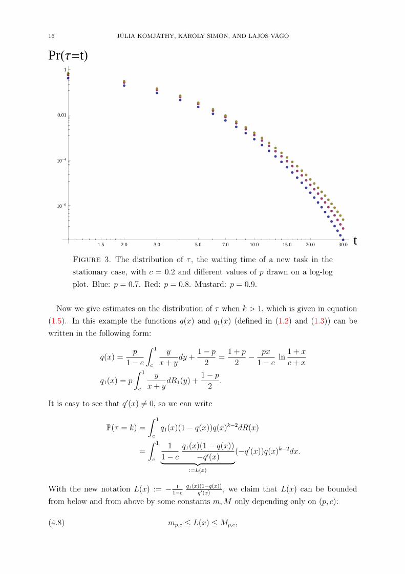
can be determined numerically, and it is represented on Fig. 1. In addition, Fig. 2 and 3illustrates the density r1(x) and the distribution of τ on a log-log plot for three differentchoice of parameters, respectively.


0.92 0.94 0.96 0.98 1.00 p

0.1

0.2

0.3

0.4

0.5

0.6

0.7

c

Figure 1. The set of parameters (p, c) where we can guarantee convergencein (4.7).

0.2 0.4 0.6 0.8 1.0 x

0.5

1.0

1.5

2.0

2.5

r1 HxL

Figure 2. The DF of the old task’s priority in the stationary case withc = 0.2 and different values of p. Blue: p = 0.7. Red: p = 0.8. Mustard:p = 0.9.


10.05.02.0 20.03.0 30.01.5 15.07.0 t

10-6

10-4

0.01

1

PrHΤ=tL

Figure 3. The distribution of τ , the waiting time of a new task in thestationary case, with c = 0.2 and different values of p drawn on a log-logplot. Blue: p = 0.7. Red: p = 0.8. Mustard: p = 0.9.

Now we give estimates on the distribution of τ when k > 1, which is given in equation(1.5). In this example the functions q(x) and q1(x) (defined in (1.2) and (1.3)) can bewritten in the following form:

q(x) =p

1− c

∫ 1

c

y

x+ ydy +

1− p2

=1 + p

2− px

1− cln

1 + x

c+ x

q1(x) = p

∫ 1

c

y

x+ ydR1(y) +

1− p2

.

It is easy to see that q′(x) 6= 0, so we can write

P(τ = k) =

∫ 1

c

q1(x)(1− q(x))q(x)k−2dR(x)

=

∫ 1

c

1

1− cq1(x)(1− q(x))

−q′(x)︸︷︷︸:=L(x)

(−q′(x))q(x)k−2dx.

With the new notation L(x) := − 11−c

q1(x)(1−q(x))q′(x)

, we claim that L(x) can be boundedfrom below and from above by some constants m,M only depending only on (p, c):

(4.8) mp,c ≤ L(x) ≤Mp,c,


since1− p

2+ pc ≤ q1(1) ≤ q1(x) ≤ 1,

1− p2

+ pc ln1

2c≤ 1− q(c) ≤ 1− q(x) ≤ 1,

1− cln 1+c

2c

≤ − 1

q′(c)≤ − 1

q′(x)≤ − 1

q′(1)

(p,c)→(1,0)−−−−−−→ ln 2 +1

2.

Thus if we set

mp,c := −q1(1)(1− q(c))(1− c)q′(1)

, and Mp, c := − 1

(1− c)q′(1).

then the bound (4.8) follows. With these bounds, one can easily estimate P(τ = k):

P(τ = k) ≤M(p, c)

∫ 1

c

q′(x)q(x)k−2dR(x) = M(p, c)1

k − 1(qk−1(c)− qk−1(1))

and similarly

P(τ = k) ≥ m(p, c)1

k − 1(qk−1(c)− qk−1(1)).

In the limit (p, c)→ (1, 0) we get

lim(p,c)→(1,0)

P(τ = k) = Ω

(1−p

2+ c ln 1

2c

ln 12c

(1− p

2+ c

))(1− (1− ln 2)k−1)

1

k − 1

Since q(c) > q(1), hence

(4.9) P(τ = k) ∼ const · 1

kqk(c) = const · 1

ke−k/k0 ,

where

k0 = − 1

ln (q(c)).

This means that the probability that the waiting time is of length k behaves approximatelyas 1

kuntil k < k0, i.e. it obeys a power law-like behavior. Furthermore, if c 6= 0 and

(p, c) → (1, 0), then k0 → ∞, i.e. the exponential cutoff in equation (4.9) shifts toinfinity, and thus for (p, c) values close to (1, 0) the distribution of τ will be close to apower-law distribution.

5. Summary

In this paper we investigated and generalized the priority queueing model of Barabási.We showed that in the original model of Barabási, the system is ergodic and irreducible asa Markov chain once the priority selection probability is separated away from 1. Further,we gave a more probabilistic approach to compute the distribution of the priority ofthe old task in the system if the buffer length equals 2, and determined the averagewaiting time of a task in the system for arbitrary buffer length. We investigated thecase p = 1 separately and found that the model is equivalent to the processes of records.Next, we generalized the priority queueing model with an arbitrary selection protocoldepending on the priorities in the system and some extra randomness. We found that


the system is ergodic and irreducible once the selection protocol is separated away from1. Further, we gave a description of the density of priority of the old task in terms ofHilbert-Schmidt operators. We investigated a special example when the priority selectionis done proportionally to the priorities of the tasks in more detail. Namely, using boundsand approximation methods based on the operator approach, we gave a region of pairs(p, c) where the Hilbert-Schmidt description of the density function is converging anddetermined the waiting time distribution in this case.

References

[1] B. C. Arnold and N. Balakrishnan and H. N. Nagaraja, Records, (2011), Wiley Series in Probabilityand Statistics.

[2] A.-L. Barabási: The origin of bursts and heavy tails in human dynamics, Nature, vol. 435, (2005),207-211.

[3] A.-L. Barabási and R. Albert: Emergence of scaling in random networks 5439, Science, vol. 286,(1999), 509-512.

[4] B. Bollobás and O. Riordan: The diameter of a scale-free random graph 1, Combinatorica, vol. 24,(2004), 5-34.

[5] B. Bollobás and O. Riordan and J. Spencer and G. Tusnády: The degree sequence of a scalefreerandom graph process 3, Random Structures Algorithms, vol. 18, (2001), 279-290.

[6] J. H. Greene, Production and Inventory Control Handbook, (1997), McGraw-Hill, New York, 3 ed.[7] R. van der Hofstad, Lecture Notes Random Graphs and Complex Networks Preprint 2012.[8] P. T. Holmes and W. E. Strawderman: A note on the waiting times between record observations 3,

Journal of Applied Probability, vol. 6, (1969), 711-714.[9] A. N. Kolmogorov and A. N. Fomin, Elements of the Theory of Functions and Functional Analysis,

vol. 1, (1981), Springer.[10] M. F. Neuts: Waiting time between record observations 1, Journal of Applied Probability, vol. 4,

(1967), 206-208.[11] P. Reynolds, ,Call Center Staffing, (2003), The Call Center School Press, Lebanon, TN.[12] W. E. Strawderman and P. T. Holmes: On the law of the iterated logarithm for inter-record times 2,

Journal of Applied Probability, vol. 7, (1970), 432-439.[13] M. N. Tata: On outstanding values in a sequence of random variables 1, Probabil-

ity Theory and Related Fields, Springer Berlin / Heidelberg, vol. 12, (1969), 9-20,http://dx.doi.org/10.1007/BF00538520.

[14] A. Vázquez: Exact results for the Barabási model of human dynamics, Physical Review Letters, vol.95, (2005), 248701.


Júlia Komjáthy, Department of Stochastics, Institute of Mathematics, Technical Uni-

versity of Budapest, 1521 Budapest, P.O.Box 91, Hungary

E-mail address: [email protected]

Károly Simon, Department of Stochastics, Institute of Mathematics, Technical Uni-

versity of Budapest, 1521 Budapest, P.O.Box 91, Hungary


Lajos Vágó, Department of Stochastics, Institute of Mathematics, Technical Univer-

sity of Budapest, 1521 Budapest, P.O.Box 91, Hungary


A GENERALIZATION OF BARABÁSI PRIORITY MODEL … · A GENERALIZATION OF BARABÁSI PRIORITY MODEL OF...

Documents

Transcript of A GENERALIZATION OF BARABÁSI PRIORITY MODEL … · A GENERALIZATION OF BARABÁSI PRIORITY MODEL OF...