A general time‐dependent stochastic method for solving Parker’stransport equation in spherical coordinates

C. Pei,1 J. W. Bieber,1 R. A. Burger,2 and J. Clem1

Received 26 May 2010; revised 10 September 2010; accepted 28 September 2010; published 11 December 2010.

[1] We present a detailed description of our newly developed stochastic approach forsolving Parker’s transport equation, which we believe is the first attempt to solve it withtime dependence in 3‐D, evolving from our 3‐D steady state stochastic approach. Ourformulation of this method is general and is valid for any type of heliospheric magneticfield, although we choose the standard Parker field as an example to illustrate the steps tocalculate the transport of galactic cosmic rays. Our 3‐D stochastic method is different fromother stochastic approaches in the literature in several ways. For example, we employspherical coordinates to integrate directly, which makes the code much more efficientby reducing coordinate transformations. What is more, the equivalence between ourstochastic differential equations and Parker’s transport equation is guaranteed by Ito’stheorem in contrast to some other approaches. We generalize the technique for calculatingparticle flux based on the pseudoparticle trajectories for steady state solutions and fortime‐dependent solutions in 3‐D. To validate our code, first we show that goodagreement exists between solutions obtained by our steady state stochastic methodand a traditional finite difference method. Then we show that good agreement alsoexists for our time‐dependent method for an idealized and simplified heliospherewhich has a Parker magnetic field and a simple initial condition for twodifferent inner boundary conditions.

Citation: Pei, C., J. W. Bieber, R. A. Burger, and J. Clem (2010), A general time‐dependent stochastic method for solvingParker’s transport equation in spherical coordinates, J. Geophys. Res., 115, A12107, doi:10.1029/2010JA015721.

1. Introduction

[2] Solar modulation is the process by which the Sunimpedes the entry of galactic cosmic rays into the solarsystem, thereby altering the intensity and energy spectrum ofthe cosmic rays. Understanding solar modulation from firstprinciples is a challenging astrophysical problem, because itrequires an understanding of the properties of magneticfields and turbulence throughout the heliosphere, while alsodemanding accurate theories for determining particle trans-port properties, such as the diffusion tensor, from theproperties of the turbulence.[3] A comprehensive understanding of solar modulation is

required for extracting information about extrasolar phe-nomena from observations of charged cosmic rays madewithin the heliosphere. For instance, consideration of mod-ulation effects is crucial for interpreting time variations ofthe antiproton/proton ratio [Bieber et al., 1999;Mitchell et al.,

2008]. Solar modulation effects must also be considered formitigation of radiation hazard from galactic cosmic rays,both for astronauts on long‐duration deep space missions,and for sensitive electronic components flown in space. Thesignificance of modulation effects is highlighted by recentobservations that the intensity of galactic cosmic rays in theinner heliosphere has risen to a new space age high[Mewaldt et al., 2009].[4] The governing equation for solar modulation is

Parker’s well‐known transport equation [Parker, 1965;Jokipii and Parker, 1970],

@f

@t¼ r � k � rf � Vfð Þ þ 1

3p2r � Vð Þ @p

3f

@p; ð1Þ

where f (r, p, t) is the omni‐directional distribution function(i.e., the phase space density averaged over solid angle inmomentum space), with p the particle momentum, r thespatial variable and V the solar wind velocity. Note that wedrop the subscript 0 typically used for the omni‐directionaldistribution function. Terms relating to the second‐orderFermi acceleration and sources will not be discussed in thispaper. The spatial diffusion tensor, k, can be decomposedinto two parts, ks, the symmetric part, and kA, the anti-symmetric part. The divergence of the antisymmetric tensor,kA, is the drift velocity, Vd. The symmetric tensor, ks,consists of the spatial diffusion parallel �k and perpendicular

1Bartol Research Institute, Department of Physics and Astronomy,University of Delaware, Newark, Delaware, USA.

2Unit for Space Physics, School of Physics, North‐West University,Potchefstroom, South Africa.

Copyright 2010 by the American Geophysical Union.0148‐0227/10/2010JA015721

JOURNAL OF GEOPHYSICAL RESEARCH, VOL. 115, A12107, doi:10.1029/2010JA015721, 2010

A12107 1 of 12

�? to the mean heliospheric magnetic field, B, which isgiven by

B ¼ A

r2er � r � r�ð ÞW�

Vsin �e�

� �1� 2H �� �

2

� �h i; ð2Þ

where A = ±B0rr02 is a constant which comes from the defi-

nition of the magnetic field, with suffix 0 indicating somereference value and the sign depending on solar cycle, andW�is the sidereal solar rotation rate corresponding to a period of25.4 days. The radius from which the field is purely radial isdenoted by r� which is usually several times the solar radiusalthough we take it to be 0 for the benchmarking againstthe finite difference method. The Heaviside step function isrepresented by H. Please note that equation (2) is only for aheliospheric magnetic field with a flat neutral sheet. Althoughour method presented here is also applicable to a wavy neutralsheet, it is too complicated to discuss here.[5] The parallel diffusion component with respect to the

magnetic field, �k, and the perpendicular component, �?,can be determined ab initio from turbulence models basedon spacecraft measurements [see, e.g., Pei et al., 2010]. Inthis paper, however, we choose three ad hoc analyticalforms for �k in order to simplify our benchmark procedure;we leave ab initio models for future publication. Theseforms are

�k ¼ �0�PBe

B; ð3Þ

�k ¼ �0�P 1þ 0:5 sin�ð ÞBe

B; or ð4Þ

�k ¼ �0�P 1þ 0:8 sin Wtð Þ½ � alternative version for time dependenceð Þ;ð5Þ

�?=�k ¼ 0:1; ð6Þwhere P is the particle rigidity, �0 is a constant, b is the ratiobetween particle speed and the speed of light, B is themagnetic field magnitude with Be its value at the Earth, and� is the azimuth angle in a heliocentric spherical coordinatesystem. The first two forms are for the benchmark of steadystate solutions. The third one is for the benchmark of time‐dependent solutions. Note that with Parker’s magnetic field,k is a function of only (r, �) in equation (4) which is not a fully3‐D function. In equation (5), k is a function of (r, �, �).[6] Two major numerical methods have been developed

to solve equation (1). One is the finite difference method, adeterministic method, employed by, e.g., Jokipii andKopriva [1979], Potgieter and Moraal [1985], and Burgerand Hattingh [1995]. In order to benchmark our newmethod, a steady state three‐dimensional finite differencemethod [Burger and Hattingh, 1995], following theapproach of Kóta and Jokipii [1983], is used in this paper.The other major method is the stochastic or Monte Carlomethod used by Jokipii and Owens [1975], Jokipii and Levy[1977], Yamada et al. [1998], Zhang [1999a, 1999b],Gervasiet al. [1999],Miyake and Yanagita [2005], Ball et al. [2005],Alanko‐Huotari et al. [2007], Bobik et al. [2008], Alanko‐Huotari et al. [2009], and Pei et al. [2009]. For 1‐D and2‐D problems, the finite difference method is much fasterthan the stochastic method. However, for fully 3‐D and

energy‐dependent problems and for a complex heliosphericmagnetic field, for example, if we consider the wavy currentsheet and the time‐dependent problem, the stochastic methodis promising because we don’t have a successful finite dif-ference method for this situation so far. In this paper weprovide a direct comparison between the results of these twomethods for different scenarios.[7] One big advantage of the stochastic method is that it is

very easy to parallelize so that it can be running on manyCPUs of a local cluster, with almost unchanged codes. Dueto the nature of this method with each random processindependent of all others, it can also be very easily adjustedto be running on distributed idle computers which canreduce the computation time and lower the hardware costsdramatically. Although this method has been investigated bymany research groups in the past, most efforts are focusedon finding the steady state solutions of equation (1). As faras we know, no 3‐D time‐dependent stochastic method hasbeen published although some work has been done for the1‐D time‐dependent case [Yamada et al., 1999; Li et al.,2009]. In this paper we present our time‐dependentmethod with a discussion of the initial conditions andboundary conditions.[8] In a related problem, the stochastic method has also

been applied to solve Roelof’s Equation [Roelof, 1969],which usually is used to describe the transport of solarenergetic particles with significant anisotropies [Kocharovet al., 1998; Zhang et al., 2009; Dröge et al., 2010]. The3‐D stochastic method introduced by Zhang et al. [2009]and Dröge et al. [2010] is applied to a modified Roelof’sEquation which includes the transport mechanisms ofstreaming, convection, pitch angle diffusion, focusing, per-pendicular diffusion, and pitch angle–dependent adiabaticcooling. This method can be easily adjusted to arbitrarymagnetic field geometries and to transport parameters thatvary spatially as well as with energy.[9] Our method described in the present manuscript is

completely adequate for the application discussed here, i.e.,the solar modulation of galactic cosmic rays. Further, themethod based upon Parker’s equation optimizes the com-puting time required to achieve the necessary accuracy inmodulation applications. It differs from the others in severaladditional ways.[10] 1. We present every step in great detail to reproduce

our results in this paper including the step transforming theoriginal Parker’s equation to the standard Fokker‐Planckequation. This step has been omitted mostly in literature butwe believe it is important when the diffusion coefficient isnot a constant (see Appendix C) in 3‐D models.[11] 2. We use spherical coordinates which is convenient

to use, for example, easy to specify boundary conditionsand the magnetic field while most other 3‐D methods[Zhang, 1999b; Ball et al., 2005] use Cartesian coordinates.Zhang [1999b] states that the integration of stochastic dif-ferential equations must be performed in terms of Cartesiancoordinates. We show, however, that for a general form forthe heliospheric magnetic field, we can actually use spher-ical coordinates directly. A more detailed discussion can befound in section 2.[12] 3. Our steady state results are strictly benchmarked

with the traditional finite difference solutions with the sameset of parameters. Our time‐dependent solutions are bench-

PEI ET AL.: TIME‐DEPENDENT STOCHASTIC METHOD A12107A12107

2 of 12

marked by Mathematica with the same boundary conditionsand initial conditions. The benchmarking results are pre-sented in section 3.

2. Stochastic Method

[13] The stochastic method to solve equation (1) can bedivided into two steps which will be illustrated in detail inthis section from 1‐D to 3‐D. The first step is that we needto find the corresponding SDEs to equation (1) based on Itoformula and solve it. The second step is that we obtain themodulated distribution function from the solutions of thecorresponding SDEs.[14] To find the corresponding SDEs, it is convenient to

transform equation (1) into the standard form of the Fokker‐Planck equation (FPE),

@F

@t¼ �

Xi

@

@qiAi q; tð ÞF½ � þ 1

2

Xi; j

@2

@qi@qjB q; tð ÞBT q; tð Þ� �

i; jF

n o;

ð7Þ

where A is a vector (though often termed the drift vector indiscussions of the stochastic method, it is not the same as thedrift velocity, Vd), and D = BBT is the diffusion tensor[Gardiner, 2004]. Note that this B is not the magnetic fieldB. Moreover, here qi denotes a generalized vector with bothspatial and momentum or energy components. The generalform for A is (Ar, A�, A�, Ap). The general form for B is afour by four matrix generally,

B ¼Brr Br� Br� Brp

B�r B�� B�� B�p

B�r B�� B�� B�p

Bpr Bp� Bp� Bpp

2664

3775:

Since second‐order acceleration mechanisms are not con-sidered, this matrix can be downgraded to a three by threematrix, i.e., the fourth row and the fourth column can beomitted. This is the case for Appendix B and Appendix C.The specific forms of A and B and the method to derivethem will be provided later in this section for 1‐D and 2‐Dmethods. For simplicity, the corresponding 3‐D forms andformulas are put in Appendix B and Appendix C.[15] The equivalent Ito stochastic differential equation is

Dq ¼ A q; tð ÞDt þ B q; tð Þ �DW; ð8Þ

which can be solved to provide the normalized transitionprobability function G(r, p, t∣re, pe, te). The normalization ofa general transition probability function isZ Z

W

ZG r; p; tjre; pe; teð Þdpd3rdt ¼ 1; ð9Þ

where W denotes the whole domain in space. G can also beinterpreted as a Green’s function [see, e.g.,Webb and Gleeson,1977; Li et al., 2009]. Here DW denotes a Wiener process(see Appendix A). The suffix e denotes the Earth or anylocation in heliosphere we are interested in. So the process tofind the corresponding set of SDEs is the process to determineA, DW, and B. For a general heliospheric magnetic field, thematrix B can be calculated according to Appendix B. In thispaper, we focus on the form of B for Parker field which is

shown in Appendix C. We show the values of A andDW for1‐D and 2‐D in section 2.1 and section 2.2. For 3‐D, thevalues of A and DW are detailed in Appendix C.[16] For all the cases, the procedures to integrate the SDEs

are similar. First, we start from some initial position, chosento be the Earth in this paper, re, and some initial time, te,integrate along the trajectory of the pseudoparticle, followthem back in time until they reach the boundary. Thebackward‐in‐time integration is more efficient than theforward‐in‐time approach because it reduces the number ofuseless pseudo‐particles although they are equivalent toeach other [Kóta, 1977]. A pseudoparticle is not a realparticle nor a test particle, but a point in phase space. A realparticle or a test particle moves around in the planetaryfield obeying Lorentz equation and following field lines [Peiet al., 2006]. A pseudoparticle has a tendency to follow fieldlines according to equation (8) provided that parallel diffu-sion dominates, but it does not in general follow them rig-orously owing to the random Wiener process present in theequation. Then we start the whole process again for anotherpseudoparticle. In this way, we have the steady state solu-tion for all the pseudoparticles. Because this is equivalentto set t → ∞, we don’t need and shouldn’t specify the initialcondition. In other words, the initial condition has no con-tribution to our solution. This can also be verified by themissing of time integral in equation (10). For the time‐dependent solution, we follow the pseudoparticle to a certainvalue of te which is not equal to infinity. The normalizedprobability function, G(r, p, t∣re, pe, te), then is calculatedbased on the trajectories we collected. Normalized proba-bility function, G, is subject to the normalization conditionthat G integrated over r and p is unity (see equation 9).[17] The set of equations in the first step is the same for

both steady state solutions and for time‐dependent solutions.However, for the second step, we must treat them differentlyto determine the modulated distribution function.[18] The modulated distribution function, f (re, pe), if we

just need the steady state solution, is determined by

f re; peð Þ ¼Ir2S

Zfb r; pð ÞG r; pjre; peð Þdpda; ð10Þ

where S denotes the boundaries which generally are closedsurfaces of a multiply connected domain and fb denotesboundary conditions. A multiply connected domain can beused to take into account of sources like Jupiter.[19] Equation (10) is a general form for steady state

solutions and for general boundaries. If the outer boundarycondition is independent of position, the integral over theouter boundary of G(r, p∣re, pe) gives G′(p∣re, pe) due to thenormalization, i.e., G′(p∣re, pe) =

Hr2SG(r, p∣re, pe)da. For

simplicity, we drop the prime. Thus if at the same time, theinner boundary is a reflecting boundary or an absorbingboundary, equation (10) reduces to

f re; peð Þ ¼Z

fouter pð ÞG pjre; peð Þdp; ð11Þ

which is a 3‐D generalization of Yamada et al. [1998,equation 6] or Li et al. [2009, equation 8], which both arefor 1‐D and for special inner boundaries only. Another pointin equation (11) is that as long as the boundary condition isindependent of position, we don’t need to know the details

PEI ET AL.: TIME‐DEPENDENT STOCHASTIC METHOD A12107A12107

3 of 12

of the final positions of “pseudo” particles on that boundaryfor any shape of the boundary. For example, even if theheliosphere has an irregular shape, such as a bullet shape, itis sufficient to know the pseudoparticle momentum when itencounters the boundary (traced backward from the Earth).Thus the integral in equation (11) can be computed directly,with no need to form the complicated function G(r, p∣re, pe)as an intermediate step.[20] The time‐dependent modulated distribution function,

f (re, pe, te), in a time‐dependent case is determined by

f re; pe; teð Þ ¼Z te

0

Ir2S tð Þ

Zfb r; p; tð ÞG r; p; tjre; pe; teð Þdpdadt

þZ Z

fi r; p; 0ð ÞGi r; p; 0jre; pe; teð Þdpd3r; ð12Þ

where fi(r, p, 0) is the initial condition. An area element onthe spatial surface is denoted by da. The integral involving figenerally is a volume integral in 3‐D. The integral involvingfb takes into account of a time‐dependent boundary condi-tion which is why we have the integral in time. The time‐dependent boundary is important in dealing with solarenergetic particles and in taking account of Jovian electrons.Gi is the Green’s function for the initial condition which hasa different unit from G. So generally speaking, after weobtained the probability function, G(r, p, t∣re, pe, te), fromthe SDEs, we need to integrate in time, in momentum, andin position over the boundary surface, to get the distributionfunction we want.[21] For a time‐dependent distribution function, f (re, pe, t),

we choose an arbitrary time interval, Dti, which satisfiesVDti �

ffiffiffiffiffiffiffiffiffiffikDti

p, then integrate the SDEs for each term

in the time series, ti = ti−1 + Dti. In order to integrateequation (12), we also need to specify an appropriate initialcondition for the time‐dependent solution, unlike the steadystate case where an initial condition is not needed.[22] In reality, this initial condition should be specified

based on observations. In this paper, for the purpose ofdemonstrating our point, we take the initial condition as

fi 0:01AU < r < 100AU; �; �; p; 0ð Þ ¼ 0: ð13Þ

This initial condition means initially at t = 0 the heliosphereis empty which implies the second integral in equation (12)vanishes. Note that the initial condition of an empty helio-sphere is different from no initial condition. At the sametime, if we use the same boundaries as we have in the steadystate solution case, the first integral in equation (12) can alsobe simplified in the same way as in equation (11). Taking allthese assumptions into account, equation (12) becomes

f re; pe; teð Þ ¼Z te

0

Zfouter pð ÞG p; tjre; peð Þdpdt: ð14Þ

[23] In this paper, we use two types of inner boundaryconditions. The first one is the reflecting boundary, namely,∂f /∂r = 0. The second one is the absorbing boundary, f = 0[Chandrasekhar, 1943]. For simplicity we take the localinterstellar intensity for protons at 100 AU, jT

LIS, as

jLIST ¼ 21:1T�2:8

1þ 5:85T�1:22 þ 1:18T�2:54sr m2 s MeV �1

; ð15Þ

where T is the kinetic energy in GeV[Webber and Higbie,2003]. This intensity is related to the omni‐directional dis-tribution function by jT = p2 f. To illustrate how to use ourstochastic method in detail, we solve equation (1) in 1‐D, 2‐D,and 3‐D step by step in sections 2.1, 2.2, and 2.3, respectively.

2.1. One‐Dimensional Stochastic Method

[24] For completeness, we will illustrate the stochasticmethod solving equation (1) in 1‐D, 2‐D, and 3‐D. The 1‐DParker’s transport equation is

@f

@t¼ 1

r2@

@rr2�rr

@f

@r

� �þ 1

3r2@

@rr2V 1

p2@

@pp3f

� 1

r2@

@rr2Vf

; ð16Þ

where r is the spatial variable, �rr the radial diffusioncoefficient.[25] In order to find the corresponding set of SDEs, it is

convenient to transform equation (16) into the standard form(equation (7)) which can be achieved by setting F = r2 f forthis 1‐D problem. Thus equation (16) can be rewritten as

@F

@t¼ � @

@rV þ 1

r 2@r 2�rr

@r

� �F

� �� @

@p3� 1

r 2@r 2V

@rp3F

� �

þ @ 2

@r 2�rrFð Þ; ð17Þ

which is in a standard form. Recognizing Dp3 = 3p2Dp,setting

q ¼ r; pf g; ð18Þ

A ¼ 1

r 2@r 2�rr

@rþ V ;� p

3r 2@r 2V

@r

�; ð19Þ

DW ¼ffiffiffiffiffiffiDt

pdwr; 0f g; ð20Þ

where DW is a Wiener process given by the standard nor-mal distribution, dwr, with a mean of zero and a standarddeviation of one which is discussed in more detail inAppendix A, and

B ¼ffiffiffiffiffiffiffiffiffi2�rr

p0

0 0

� �; ð21Þ

we obtain the corresponding SDEs following fromequation (8),

Dr ¼ 1

r 2@r 2�rr

@rþ V

� �Dt þ

ffiffiffiffiffiffiffiffiffiffiffiffiffiffi2�rrDt

pdwr; ð22Þ

Dp ¼ � p

3r2@r2V

@rDt: ð23Þ

[26] To find the steady state solution, we integrate theSDEs approximately to t → ∞. Usually, this can be done bychoosing a large value for time, say, 1 year for 10 MeVprotons. The modulated distribution function f (re, pe) at re =1 AU and at p = pe, is determined by equation (10) orequation (11). For the time‐dependent solution, we integrate

PEI ET AL.: TIME‐DEPENDENT STOCHASTIC METHOD A12107A12107

4 of 12

the SDEs to a fixed time, te. The time‐dependent modulateddistribution function f (re, pe, te) at re = 1 AU and at p = pe, isdetermined by equation (12) or equation (14). We willrepeat this again for 2‐D and 3‐D in this paper since thisprocedure is the same for 2‐D and 3‐D.

2.2. Two‐Dimensional Stochastic Method

[27] For simplicity and for the purpose of benchmarking,let us discuss the 2‐D stochastic method without consideringdrift and cross terms of k which have been ignored in manypapers. With these simplifications, according to equation (1),the 2‐D transport of cosmic rays in the heliosphere is,

@f

@t¼ 1

r2@

@rr2�rr

@f

@r

� �þ 1

r2 sin �

@

@���� sin �

@f

@�

� �

þ 1

r2@

@rr2V @

@p3p3f � 1

r2@

@rr2Vf

; ð24Þ

with (r, �) the spatial variables in polar coordinates.[28] Just as in the 1‐D case, it is necessary to transform

equation (24) to the standard form given in equation (7). Inthe literature, there are two different ways to do that. Forexample, by defining m = cos �, the FPE is

@f

@t¼ 1

r2@

@r

@

@rr2�rrf � 1

r2@

@rf@r2�rr

@r

� �þ @

@�

@

@�

� 1� �2 ���

r2f

h i� @

@�f@

@�1� �2 ���

r2

h i �

þ @

@p31

r2@r2V

@rp3f

� �� 1

r2@

@rr2Vf

: ð25Þ

[29] By setting F = r2f [Alanko‐Huotari et al., 2007;Bobik et al., 2008], equation (25) can be rewritten as

@F

@t¼ � @

@rVFð Þ � @

@rF1

r2@r2�rr

@r

� �� @

@�F

@

@�1� �2 ���

r2

h i �

� @

@p3� 1

r2@r2V

@rp3F

� �þ @

@r

@

@r�rrFð Þ

þ @

@�

@

@�1� �2 ���

r2F

h i: ð26Þ

[30] In this case, setting

q ¼ r; �; pf g; ð27Þ

A ¼ 1

r2@r2�rr

@rþ V ;

@

@�

1� �2ð Þ���

r2

� �; � p

3r2@r2V

@r

�; ð28Þ

DW ¼ffiffiffiffiffiffiDt

pdwr; dw�; 0� �

; ð29Þ

where DW is a Wiener process given by the standard nor-mal distribution with a mean of zero and a standard devia-tion of one and

B ¼ffiffiffiffiffiffiffiffiffi2�rr

p0 0

0 1r

ffiffiffiffiffiffiffiffiffiffiffiffiffiffiffiffiffiffiffiffiffiffiffiffiffiffi2 1� �2ð Þ���

p0

0 0 0

24

35; ð30Þ

we find the corresponding SDEs for this transformationaccording to Ito’s theorem are

Dr ¼ 1

r2@r2�rr

@rþ V

� �Dt þ

ffiffiffiffiffiffiffiffiffiffiffiffiffiffi2�rrDt

pdwr; ð31Þ

D� ¼ @

@�

1� �2ð Þ���

r2

� �Dt þ 1

r

ffiffiffiffiffiffiffiffiffiffiffiffiffiffiffiffiffiffiffiffiffiffiffiffiffiffiffiffiffiffiffi2 1� �2ð Þ���Dt

pdw�; ð32Þ

Dp ¼ � p

3r2@r2V

@rDt: ð33Þ

[31] Jokipii and Levy [1977] used another formula, i.e.,F = sin �r2f. The corresponding FPE in this case is

@F

@t¼ @

@r

@

@r�rrFð Þ � @

@rF1

r2@r2�rr

@r

� �� @

@rVFð Þ

þ @

@�

@

@�

���

r2F

� �� @

@�F

1

r2 sin �

@ sin ����

@�

� �

þ @

@p31

r2@r2V

@rp3F

� �: ð34Þ

[32] Similarly, the corresponding SDEs are

Dr ¼ 1

r2@r2�rr

@rþ V

� �Dt þ

ffiffiffiffiffiffiffiffiffiffiffiffiffiffi2�rrDt

pdwr; ð35Þ

D� ¼ 1

r2 sin �

@ sin ����

@�

� �Dt þ 1

r

ffiffiffiffiffiffiffiffiffiffiffiffiffiffi2���Dt

pdw�; ð36Þ

Dp ¼ � p

3r2@r2V

@rDt: ð37Þ

[33] Actually, without explicitly using Ito’s theorem,Jokipii and Levy [1977] immediately realize that transitionmoments satisfy the equations, hDr2i = 2�rrDt, hD�2i =2���Dt/r2, hDri = (2�rr /r + V)Dt, hD�i = ��� cot�Dt/r2,hDpi = − 2VpDt/3r, which follows from a comparison ofequation (34) with the FPE in the work by Chandrasekhar[1943, equation 223]. Therefore we can integrate the cor-responding SDEs directly in polar coordinates withouttransforming them into Cartesian coordinates. See section 3for more details.[34] We have shown that there are two different sets of

SDEs, according to different transformations in order toreach the standard form of FPE. However, it turns out thatthese two approaches yield the same results (see Figure 1and section 3 for more details).

2.3. Three‐Dimensional Stochastic Method

[35] For 3‐D modulation of cosmic rays in the helio-sphere, we consider three different scenarios for the com-parison of the finite difference method and the stochasticmethod. The first one is 3‐D without drift effects and k withcross terms (such as �r� [see, e.g., Burger et al., 2008])suppressed (see Figure 2). The transformation from field‐aligned to heliocentric spherical coordinates, for a general

PEI ET AL.: TIME‐DEPENDENT STOCHASTIC METHOD A12107A12107

5 of 12

three‐dimensional form of the heliospheric magnetic field, isgiven by Burger et al. [2008]. The FPE in this case is

@f

@t¼ 1

r2@

@rr2�rr

@f

@r

� �þ 1

r2 sin �

@

@���� sin �

@f

@�

� �þ 1

r2 sin2 �

@

@�

� ���@f

@�

� �þ 1

r2@

@rr2V @

@p3p3f � 1

r2@

@rr2Vf

: ð38Þ

The corresponding SDEs are

Dr ¼ 1

r2@r2�rr

@rþ V

� �Dt þ

ffiffiffiffiffiffiffiffiffiffiffiffiffiffi2�rrDt

pdwr; ð39Þ

D� ¼ 1

r2 sin �

@ sin ����

@�Dt þ 1

r

ffiffiffiffiffiffiffiffiffiffiffiffiffiffi2���Dt

pdw�; ð40Þ

D� ¼ 1

r2 sin2 �

@���

@�Dt þ 1

r sin �

ffiffiffiffiffiffiffiffiffiffiffiffiffiffiffi2���Dt

pdw�; ð41Þ

Dp ¼ � p

3r2@r2V

@rDt: ð42Þ

[36] The second one is 3‐D without drift effects but kwith cross terms. Here we assume �r� = ��r and the order ofall the derivatives are exchangeable.

@f

@t¼ 1

r2@

@rr2�rr

@f

@r

� �þ 1

r2 sin �

@

@���� sin �

@f

@�

� �þ 1

r2 sin2 �

@

@�

� ���@f

@�

� �þ 1

r sin �

@

@���r

@f

@r

� �þ 1

r2 sin �

@

@rr�r�

@f

@�

� �

þ 1

r2@

@rr2V @

@p3p3f � 1

r2@

@rr2Vf

: ð43Þ

The corresponding SDEs are

Dr ¼ 1

r2@r2�rr

@rþ 1

r sin �

@�r�

@�þ V

� �Dt þ B �DW½ �r; ð44Þ

D� ¼ 1

r2 sin �

@ sin ����

@�Dt þ B �DW½ ��; ð45Þ

D� ¼ 1

r2 sin2 �

@���

@�þ 1

r2 sin �

@r�r�

@rDt þ B �DW½ ��; ð46Þ

Dp ¼ � p

3r2@r2V

@rDt: ð47Þ

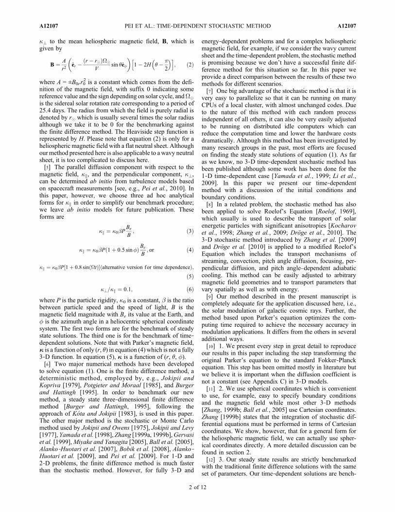
The calculation of B in this scenario is listed in theAppendix C.[37] The last scenario is a fully 3‐D model with drift

effects and a fully 3‐D k tensor including cross terms (seeFigures 3, 4, and 5). The general weak scattering driftvelocity of a particle with charge q, momentum p, and speedv is given by Jokipii et al. [1977] for the case of a flatcurrent sheet inside the equatorial plane,

Vd ¼ pv

3qr� B

B2

� �¼ 2pvr

3qA 1þ �2ð Þ2 1� 2H �� �

2

� �h i

� � �

tan �er þ 2þ �2

�e� þ �2

tan �e�

� �þ 2pvr

3qA 1þ �2ð Þ� �� �

2

� ��er þ e�

; ð48Þ

where g = rW� sin �/V. For the current sheet drift, we didnot use the last term in the form given but adopted a formulafollowing from a result by Burger et al. [1985] and Burger[1987] for the drift along the current sheet,

Vdc ¼ 0:457� 0:412dj jRg

þ 0:0915dj j2R2g

!v; ð49Þ

Figure 1. Benchmark for the 2‐D steady state method. Thesolid line is the LIS. The dashed line denotes the finite differ-ence method results [Burger and Hattingh, 1995]. The crossesdenote results using Bobik et al.’s [2008] formulas (equations(31)–(33)), and the open circles denote results using Jokipiiand Levy’s [1977] formulas (equations (35)–(37)).

Figure 2. Benchmark for the 3‐D steady state method forthe first scenario of section 2.3 without drift and withoutcross terms in the diffusion tensor. The circles denote ourstochastic results, and the dashed line denotes the our finitedifference results.

PEI ET AL.: TIME‐DEPENDENT STOCHASTIC METHOD A12107A12107

6 of 12

where d is the distance to the current sheet and Rg is theLarmor radius. This formula is valid when d is smaller than2 times Rg.[38] Parker’s transport equation in this case is

@f

@t¼ 1

r2@

@rr2�rr

@f

@r

� �þ 1

r2 sin �

@

@���� sin �

@f

@�

� �

þ 1

r2 sin2 �

@

@����

@f

@�

� �þ 1

r sin �

@

@���r

@f

@r

� �

þ 1

r2 sin �

@

@rr�r�

@f

@�

� �þ 1

r2@

@rr2V @

@p3p3f

� 1

r2@

@rr2Vf � 1

r2@

@rr2Vdrf

� 1

r sin �

@

@�sin �Vd�fð Þ � 1

r sin �

@

@�Vd�f

: ð50Þ

The corresponding SDEs are

Dr ¼ 1

r2@r2�rr

@rþ 1

r sin �

@�r�

@�þ V þ Vdr

� �Dt þ B �DW½ �r;

ð51Þ

D� ¼ 1

r2 sin �

@ sin ����

@�Dt þ Vd�

rDt þ B �DW½ ��; ð52Þ

D� ¼ 1

r2 sin2 �

@���

@�þ 1

r2 sin �

@r�r�

@rDt þ Vd�

r sin �Dt þ B �DW½ ��;

ð53Þ

Dp ¼ � p

3r2@r2V

@rDt: ð54Þ

The calculation of B can be done similarly as in the lastscenario.

3. Benchmarks

3.1. Benchmarks for Steady State Solutions

[39] Because Yamada et al. [1998] already benchmarkedthe 1‐D steady state solution with a Crank‐Nicholsonmethod, we start the benchmark with the 2‐D steady state

Figure 3. Benchmark for the 3‐D steady state method for the third scenario in section 2.3 with �kspecified by equation (4). As in Figure 2, the circles denote our stochastic results. Red and dark blue linesdenote the our finite difference results. Red denotes the results for qA > 0, and dark blue denotes qA < 0.

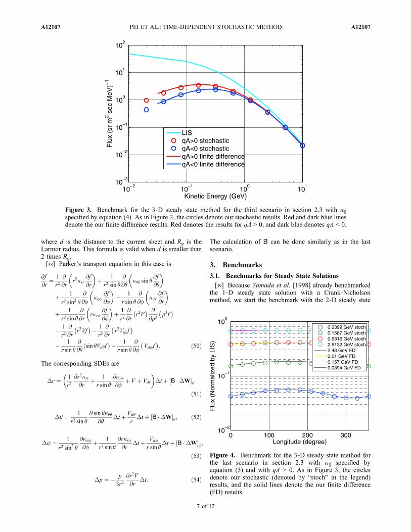
Figure 4. Benchmark for the 3‐D steady state method forthe last scenario in section 2.3 with �k specified byequation (5) and with qA > 0. As in Figure 3, the circlesdenote our stochastic (denoted by “stoch” in the legend)results, and the solid lines denote the our finite difference(FD) results.

PEI ET AL.: TIME‐DEPENDENT STOCHASTIC METHOD A12107A12107

7 of 12

solution. The benchmarks for 2‐D steady state results areshown in Figure 1. The solid line is the local interstellarspectrum (LIS). The dashed line denotes the finite differencemethod results [Burger and Hattingh, 1995]. The crossesdenote results using the first formula equations (31)–(33)[Bobik et al., 2008], and the open circles are for resultsusing the second formula equations (35)–(37) [Jokipii andLevy, 1977]. Here we use equation (4) for � with �0 = 2 ×1023 cm2sec−1GV−1. Obviously, Figure 1 shows that thesetwo different stochastic methods are in agreement. Thereason for this is that the eigenvalues and the normalizedeigenvectors for these SDEs are identical. Further the twostochastic approaches yield almost identical results to thefinite difference method. We emphasize that these results areobtained by integrating the SDEs in polar coordinates, not inthe Euclidean space. Therefore, this benchmark also vali-dated our approach.[40] The benchmark for 3‐D steady state results are shown

in Figures 2–5. Figure 2 is for the first scenario without driftand without cross terms in the diffusion tensor. The paralleldiffusion coefficient �k is specified by equation (4), where�0 = 1 × 1022 cm2sec−1GV−1. The LIS is denoted by the blueline in Figure 2. The finite difference method result is pre-sented by the green dotted line, and the red open circles areour stochastic results. The agreement between these resultsis excellent (within 1%) for the two different methods.[41] Figures 3–5 show the benchmark for the third sce-

nario in section 2.3 (although not shown, we have per-formed benchmarks for the second scenario and manyothers). Figure 3 is for � specified by equation (4). Figures 4and 5 are for �k specified by equation (5). For both cases, �0 =1 × 1022cm2sec−1GV−1 In Figure 3, for qA > 0, the relativedifference between the stochastic result and the finite differ-ence result is better than 10%. For qA < 0, the relative dif-ference is better than 5%. Figures 4 and 5 are for a fully 3‐Dscenario. Herek is also a function of azimuth �, and we showthe normalized intensity at different longitudes in this plot.

The agreements are good for qA > 0 and for qA < 0. Weobserve that the highest value of �k in equation (5) is at azi-muth � = 90°. However, the peak intensities in Figures 4 and5 are shifted to values higher than 90° owing to the spiralstructure of the Parker field.

3.2. Benchmarks for Time‐Dependent Solutions

[42] So far all the benchmarks are for the steady statesolutions taking advantage of the finite difference codes inour group. However, we don’t have this luxury to bench-mark the time‐dependent stochastic method in this way. Butfor simpler problems, other tools, like Mathematica, canprovide us accurate solutions. Thus we seek a way tobenchmark our method by using Mathematica to solve asimpler diffusion equation without losing the generality.[43] Because the SDEs for the steady state method and for

the time‐dependent method are exactly the same, thebenchmarks for the steady state solutions are also thebenchmarks for the first step, solving the SDEs, in the time‐dependent method. Thus we only need to benchmark thesecond step, obtaining the spectrum from the probabilityfunction by using equation (12), for the time‐dependentmethod. So we use our time‐dependent method to solvesimpler problems which Mathematica can provide solutionsfor us to benchmark the second step. In all the cases dis-cussed in this section, we use an initial condition specifiedby equation (13). Physically, this corresponds to a situationin which the “heliosphere” is initially empty of cosmic rays,while the LIS illuminates the boundary. Our time‐dependentsolutions track how GCRs gradually fill the heliosphere withthe passage of time if diffusion is the only process thatoccurs.[44] The diffusion equation for the purpose of bench-

marking is

@u

@t¼ k � #2u; ð55Þ

where k = �0 [1 + 0.8 sin (W�t)].

Figure 5. Benchmark for the 3‐D steady state method forthe last scenario in section 2.3 with �k specified byequation (5) and with qA < 0. As in Figure 3, the circlesdenote our stochastic results, and the solid lines denote theour finite difference results.

Figure 6. Mathematica solution for 1‐D time‐dependentdiffusion with the reflecting inner boundary.

PEI ET AL.: TIME‐DEPENDENT STOCHASTIC METHOD A12107A12107

8 of 12

[45] Figure 6 shows the Mathematica 1‐D solution for thereflecting inner boundary, ∂ u/∂ r = 0 at r = 0, with timefrom 0 to 200 days. The outer boundary is specified asu(100,t) = 1. Figure 7 is the Mathematica 1‐D solution forabsorbing inner boundary, u(0,t) = 0, with time from 0 to100 days. Other parameters are the same as those in Figure 6.These show the role of inner boundary condition is impor-tant in 1‐D solutions. With the reflecting inner boundary,the heliosphere asymptotically becomes filled with cosmicrays at the level of the LIS, while for the absorbing innerboundary the asymptotic state is a uniform density gradient.[46] The 1‐D benchmarks are shown in Figures 8 and 9.

The blue dotted line is the Mathematica 1‐D solution. Theopen red circles denote our stochastic results for the re-flecting inner boundary. The red dots denote our stochasticresults for the absorbing inner boundary. Agreement is so

good that the blue line is partially obscured by the stochastic(red) solution. Note that the scale of the y axis is different forthe plots in Figures 8 and 9, which is the reason that thestatistic behavior of our solution in Figure 9 is more evident.Especially for the reflecting boundary case, the 25.4 dayperiod is clearly shown in both results.[47] The 2‐D and 3‐D benchmarks are shown in Figures 10

and 11. The blue lines denote the Mathematica solutions. Thered circles denote our stochastic results. These are all for re-flecting inner boundaries. To be specific, for 2‐D diffusion,the boundary conditions are

@u

@xjx¼0 ¼ 0; ð56Þ

@u

@yjy¼0 ¼ 0; ð57Þ

u 100; y; tð Þ ¼ 1; ð58Þ

Figure 7. Mathematica solution for 1‐D time‐dependentdiffusion with the absorbing inner boundary.

Figure 8. Benchmarks for 1‐D time‐dependent methodwith the reflecting inner boundary. The blue dotted line de-notes the Mathematica solution with the same set of para-meters. The open red circles denote our stochastic results.

Figure 9. Benchmarks for 1‐D time‐dependent methodwith the absorbing inner boundary. The blue dotted line de-notes the Mathematica solution with the same set of para-meters. The red dots denote our stochastic results.

Figure 10. Benchmarks for 2‐D time‐dependent methodwith reflecting inner boundaries. The blue line denotes theMathematica solution with the same set of parameters.The open red circles denote our stochastic results.

PEI ET AL.: TIME‐DEPENDENT STOCHASTIC METHOD A12107A12107

9 of 12

u x; 100; tð Þ ¼ 1: ð59Þ

For 3‐D, the boundary conditions are

@u

@xjx¼0 ¼ 0; ð60Þ

@u

@yjy¼0 ¼ 0; ð61Þ

@u

@zjz¼0 ¼ 0; ð62Þ

u 100; y; z; tð Þ ¼ 1; ð63Þ

u x; 100; z; tð Þ ¼ 1; ð64Þ

u x; y; 100; tð Þ ¼ 1: ð65Þ

The good agreement between our results with the Mathe-matica results proves that the second step in our time‐dependent method is correct. Note that for the time neededto reach quasi‐equilibrium for 1‐D, 2‐D, or 3‐D is differentin the reflecting inner boundary case. For 1‐D, it takes about200 days, 2‐D about 100 days, and 3‐D about 80 days. Thecomputation time for a time‐dependent solver in thesebenchmarks is several minutes on one CPU. To be morespecific, let us take the 3‐D case as an example, we employ9000 particles for one energy level with the time step of 100 s.For a 100 day solution, which is the last point in Figure 11,the codes take about 7 min to finish on one of the CPUs of adual‐core INTEL E6850.

4. Conclusions and Future Work

[48] We present detailed benchmarks for our fully three‐dimensional method for steady state solution as well as

time‐dependent solutions. For the steady state solutions, weshow that the agreement between our stochastic results andthe finite difference results is excellent. But our steady statemethod is different from any other 3‐D method by using adifferent set of SDEs and by integrating the SDEs inspherical coordinates directly. Our steady state method can beviewed as an extension from Jokipii and Levy [1977] (2‐D) to3‐D. For the time‐dependent method, we benchmark it in twosteps. The benchmarks for the steady state solution serve asthe first step since the two methods use the exactly the sameset of SDEs. The second step is done by employing Math-ematica to solve a simple diffusion equation. As far as weknow, our time‐dependent method is the first of its kind.Although there are other time‐dependent methods have beenpublished, for example, by Yamada et al. [1999] and Li et al.[2009], they are time‐dependent solvers only for onedimensional in space. Our method is also the only 3‐Dmethod that has been thoroughly benchmarked in the literature.[49] This stochastic method is based on the assumption

that each random process is independent of every other one.Therefore, it is suitable for parallel computing and distrib-uted computing. Currently, our code is running in parallel.To use more idle computer resources, distributed computingis promising too. Also important is that almost 100 percentof the code can be parallelized which means we can speedup the calculation more significantly. With the advantage ofusing parallel computing and distributed computing, webelieve a new era for the stochastic method has dawned.

Appendix A: Wiener Process

[50] In the stochastic equations, DW satisfies a Wiener(also called Wiener‐Lévy) process, which is a nonstationaryMarkov process that has a Gaussian distribution [see, e.g.,Gardiner, 2004]

p W tð Þ; tjW t0ð Þ; t0ð Þ ¼ 1ffiffiffiffiffiffiffiffiffiffiffiffiffiffiffiffiffiffiffiffi2� t � t0ð Þp e� Wi tð Þ�Wi t0ð Þ½ �2=2= t�t0ð Þ; ðA1Þ

or equivalently

p DWið Þ ¼ 1ffiffiffiffiffiffiffiffiffiffiffi2�Dt

p e�DW 2i =2=Dt : ðA2Þ

[51] What we use in our calculation is a normalizedGaussian distribution with a mean of zero and a standarddeviation of one,

p Dwið Þ ¼ 1ffiffiffiffiffiffi2�

p e�Dw2i =2: ðA3Þ

It is easily shown that a Wiener process is self‐similar in thesense that

DWi Dtð Þ ¼ �1=2DWi Dtð Þ; ðA4Þ

Figure 11. Benchmarks for 3‐D time‐dependent methodwith reflecting inner boundaries. As in Figure 10, the blueline denotes the Mathematica solution with the same set ofparameters. The open red circles denote our stochastic results.

PEI ET AL.: TIME‐DEPENDENT STOCHASTIC METHOD A12107A12107

10 of 12

and consequently

DWi Dtð Þ ¼ffiffiffiffiffiffiDt

pDwi: ðA5Þ

Appendix B: General Form of Matrix B in 3‐D

[52] The general form of the matrix B satisfies

BBT ¼

2�rr2�r�

r

2�r�

r sin �2�r�

r

2���

r22���

r2 sin �2�r�

r sin �

2���

r2 sin �

2���

r2 sin2 �

26666664

37777775: ðB1Þ

The real B exists if Matrix B1 is positive definite, and this istrue since the diffusion coefficients parallel and perpendic-ular to the background field are positive by definition. For ageneral field with a meridional component, like Fisk‐typefields [Fisk, 1996; Burger and Hitge, 2004], a possibility forB is

which means that our method in this paper mainly for Parkerfield can be extended for other heliospheric magnetic fields.[53] For Parker‐type fields, without a meridional compo-

nent and consequently �r� = ��� = 0, B can be simplified to

B ¼

ffiffiffiffiffiffiffiffiffiffiffiffiffiffiffiffiffiffiffiffiffiffiffi2�rr �

2�2r�

���

s0

ffiffiffi2

p�r�ffiffiffiffiffiffiffiffi���

p

0

ffiffiffiffiffiffiffiffiffi2���

pr

0

0 0

ffiffiffiffiffiffiffiffiffiffi2���

pr sin �

266666664

377777775: ðB2Þ

This matrix is not unique and an alternative as used in thispaper is given in Appendix C.

Appendix C: Matrix B for Parker Field

[54] To determine the matrix, B, in equations (44)–(47),we need to decompose the following matrix D,

BBT ¼2�rr 0

2�r�

r sin �

02���

r20

2��r

r sin �0

2���

r2 sin2 �

2666664

3777775;

into a product of two matrices, such as D = BBT.[55] Since this matrix is positive definite and symmetric, the

eigenvalues of this matrix are positive. The eigenvalues are

l ¼

�rr þ ���

r2 sin2 ��

ffiffiffiffiffiffiffiffiffiffiffiffiffiffiffiffiffiffiffiffiffiffiffiffiffiffiffiffiffiffiffiffiffiffiffiffiffiffiffiffiffiffiffiffiffiffiffiffiffiffiffiffiffiffiffiffiffiffiffiffi���

r2 sin2 �� �rr

� �2

þ 2�r�

r sin �

� �2s

2���r2

�rr þ ���

r2 sin2 �þ

ffiffiffiffiffiffiffiffiffiffiffiffiffiffiffiffiffiffiffiffiffiffiffiffiffiffiffiffiffiffiffiffiffiffiffiffiffiffiffiffiffiffiffiffiffiffiffiffiffiffiffiffiffiffiffiffiffiffiffiffi���

r2 sin2 �� �rr

� �2

þ 2�r�

r sin �

� �2s

2666666664

3777777775:

If we define

a ¼ �rr � ���

r2 sin2 �;

b ¼ 2�r�

r sin �;

c ¼ �rr þ ���

r2 sin2 �;

the corresponding eigenvectors are,

1b a� ffiffiffiffiffiffiffiffiffiffiffiffiffiffiffi

a2 þ b2p

0 1b a� ffiffiffiffiffiffiffiffiffiffiffiffiffiffiffi

a2 þ b2p

0 1 01 0 1

24

35: ðC1Þ

Thus the matrix B is

ffiffiffiffiffiffiffiffiffiffiffiffiffiffiffiffiffiffiffiffiffiffiffiffiffiffiffiffiffiffiffiffiffiffiffiffiffiffiffiffiffiffiffiffiffiffiffiffiffiffiffiffiffiffiffiffiffiffiffiffiffiffiffiffiffiffiffiffiffiffiffiffiffiffiffiffiffiffiffiffiffiffiffiffiffiffiffiffiffiffiffiffiffiffiffiffiffiffiffiffiffiffi����

2r� � 2�r��r���� þ �rr�

2�� þ ����

2r� � �rr������

0:5 �2�� � ������

� �vuut �r���� � �r����

�2�� � ������

ffiffiffiffiffiffiffiffiffiffiffiffiffiffiffiffiffiffiffiffiffiffiffiffiffiffiffiffiffiffiffi2��� �

2�2��

���

!vuut ffiffiffi2

p�r�ffiffiffiffiffiffiffiffi���

p

0

ffiffiffiffiffiffiffiffiffiffiffiffiffiffiffiffiffiffiffiffiffiffiffiffiffiffiffiffiffiffiffiffiffiffiffiffiffi2 ��� � �2

��=���

� �rr

���

r

ffiffiffiffiffiffiffiffi2

���

s

0 0

ffiffiffiffiffiffiffiffiffiffi2���

pr sin �

26666666666664

37777777777775;

�b a� ffiffiffiffiffiffiffiffiffiffiffiffiffiffiffi

a2 þ b2p ffiffiffiffiffiffiffiffiffiffiffiffiffiffiffiffiffiffiffiffiffiffiffiffiffiffiffi

c� ffiffiffiffiffiffiffiffiffiffiffiffiffiffiffia2 þ b2

pp0 �

b aþ ffiffiffiffiffiffiffiffiffiffiffiffiffiffiffia2 þ b2

p ffiffiffiffiffiffiffiffiffiffiffiffiffiffiffiffiffiffiffiffiffiffiffiffiffiffifficþ ffiffiffiffiffiffiffiffiffiffiffiffiffiffiffi

a2 þ b2pp

0 1 0

�ffiffiffiffiffiffiffiffiffiffiffiffiffiffiffiffiffiffiffiffiffiffiffiffiffiffiffic� ffiffiffiffiffiffiffiffiffiffiffiffiffiffiffi

a2 þ b2pp

0 �ffiffiffiffiffiffiffiffiffiffiffiffiffiffiffiffiffiffiffiffiffiffiffiffiffiffifficþ ffiffiffiffiffiffiffiffiffiffiffiffiffiffiffi

a2 þ b2pp

266664

377775; ðC2Þ

PEI ET AL.: TIME‐DEPENDENT STOCHASTIC METHOD A12107A12107

11 of 12

where a and b come from the normalization of theeigenvectors.[56] By setting

q ¼ r; �; �; pf g; ðC3Þ

A ¼ 1

r2@r2�rr

@rþ 1

r sin �

@�r�

@�þ V þ vdr

;

1

r2 sin �

@ sin ����

@�þ vd�

r;

1

r2 sin2 �

@���

@�þ 1

r2 sin �

@r�r�

@rþ vd�r sin �

;� p

3r2@r2V

@r

�; ðC4Þ

DW ¼ffiffiffiffiffiffiDt

pdwr; dw�; dw�; 0� �

; ðC5Þ

we obtain the equations (44)–(47). The procedures to cal-culate matrix B for equations (51)–(54) are similar.

[57] Acknowledgments. This work was supported in part by NASAGuest Investigator grant NNX07AH73G, NASA Heliophysics Theorygrant NNX08AI47G, the Charged Sign Dependence grant NNG05WC08G,and the South African National Research Foundation. R. A. Burger thanksI. Burger for many useful discussions on SDEs.[58] Philippa Browning thanks the reviewers for their assistance in

evaluating this manuscript.

ReferencesAlanko‐Huotari, K., I. G. Usoskin, K. Mursula, and G. A. Kovaltsov(2007), Stochastic simulation of cosmic ray modulation including a wavyheliospheric current sheet, J. Geophys. Res., 112, A08101, doi:10.1029/2007JA012280.

Alanko‐Huotari, K., I. G. Usoskin, K. Mursula, and G. A. Kovaltsov(2009), Correction to “Stochastic simulation of cosmic ray modulationincluding a wavy heliospheric current sheet,” J. Geophys. Res., 114,A03101, doi:10.1029/2008JA013919.

Ball, B., M. Zhang, H. Rassoul, and T. Linde (2005), Galactic cosmic‐raymodulation using a solar minimum MHD heliosphere: A stochastic par-ticle approach, Astrophys. J., 634, 1116–1125.

Bieber, J.W., R. A. Burger, R. Engel, T. K. Gaisser, S. Roesler, and T. Stanev(1999), Antiprotons at solar saximum, Phys. Rev. Lett., 83, 674–677.

Bobik, P., K. Kudela, M. Boschini, D. Grandi, M. Gervasi, and P. G. Rancoita(2008), Solar modulation model with reentrant particles, Adv. Space Res.,41, 339–342.

Burger, R. A. (1987), On the theory and application of drift motion ofcharged particles in inhomogeneous magnetic fields, Ph.D. thesis, Potch-efstroomse Univ. vir Christelike Hoër Onderwys, Potchefstroomse, SouthAfrica.

Burger, R. A., and M. Hattingh (1995), Steady‐state drift‐dominatedmodulation models for galactic cosmic rays, Astrophys. Space Sci.,230, 375–382.

Burger, R. A., and M. Hitge (2004), The effect of a fisk‐type heliosphericmagnetic field on cosmic‐ray modulation, Astrophys. J., 617, L73–L76.

Burger, R. A., H. Moraal, and G. M. Webb (1985), Drift theory of chargedparticles in electric and magnetic fields, Astrophys. Space Sci., 116,107–129.

Burger, R. A., T. P. J. Krüger, M. Hitge, and N. E. Engelbrecht (2008), Afisk‐parker hybrid heliospheric magnetic field with a solar‐cycle depen-dence, Astrophys. J., 674, 511–519.

Chandrasekhar, S. (1943), Stochastic problems in physics and astronomy,Rev. Mod. Phys., 15, 1–89.

Dröge,W., Y. Y. Kartavykh, B. Klecker, andG. A. Kovaltsov (2010), Aniso-tropic three‐dimensional focused transport of solar energetic particles inthe inner heliosphere, Astrophys. J., 709, 912–919.

Fisk, L. A. (1996), Motion of the footpoints of heliospheric magnetic fieldlines at the Sun: Implications for recurrent energetic particle events athigh heliographic latitudes, J. Geophys. Res., 101, 15,547–15,554.

Gardiner, C. W. (2004), Handbook of Stochastic Methods for Physics,Chemistry and the Natural Sciences, 3rd ed., Springer, Berlin.

Gervasi, M., P. G. Rancoita, I. G. Usoskin, and G. A. Kovaltsov (1999),Monte‐Carlo approach to galactic cosmic ray propagation in the helio-sphere, Nucl. Phys. B Proc. Suppl., 78, 26–31.

Jokipii, J. R., and D. A. Kopriva (1979), Effects of particle drift on thetransport of cosmic rays. III. Numerical models of galactic cosmic‐raymodulation, Astrophys. J., 234, 384–392.

Jokipii, J. R., and E. H. Levy (1977), Effects of particle drifts on the solarmodulation of galactic cosmic rays, Astrophys. J., 213, L85–L88.

Jokipii, J. R., and A. J. Owens (1975), Implications of observed chargestates of low‐energy solar cosmic rays, J. Geophys. Res., 80, 1209–1212.

Jokipii, J. R., and E. N. Parker (1970), On the convection, diffusion, andadiabatic deceleration of cosmic rays in the solar wind, Astrophys. J.,160, 735–744.

Jokipii, J. R., E. H. Levy, and W. B. Hubbard (1977), Effects of particledrift on cosmic‐ray transport. I. General properties, application to solarmodulation, Astrophys. J., 213, 861–868.

Kocharov, L., R. Vainio, G. A. Kovaltsov, and J. Torsti (1998), Adiabaticdeceleration of solar energetic particles as deduced from Monte Carlosimulations of interplanetary transport, Solar Phys., 182, 195–215.

Kóta, J. (1977), Energy loss in the solar system and modulation of cosmicradiation, Contrib. Int. Cosmic Ray Conf. IUPAP 15th, vol. 11, 186–191.

Kóta, J., and J. R. Jokipii (1983), Effects of drift on the transport of cosmicrays. VI. A three‐dimensional model including diffusion, Astrophys. J.,265, 573–581.

Li, G., et al. (2009), Modeling the transport of cosmic ray due to long‐termvariation using a stochastic differential method, paper presented at 31stInternational Cosmic Ray Conference, Univ. of Łódź, Łódź, Poland,7–15 Jul.

Mewaldt, R. A., et al. (2009), Galactic cosmic ray intensities reach recordlevels in 2009, Eos Trans. AGU, 90(52), Fall Meet. Suppl., AbstractSH13C‐08.

Mitchell, J. W., et al. (2008), Solar modulation of low‐energy antiprotonand proton spectra measured by BESS, in Proceedings of the 30thInternational Cosmic Ray Conference, vol. 1, edited by R. Caballeroet al., pp. 455–458, Univ. Nac. Auton. de Mexico, Mexico City.

Miyake, S., and S. Yanagita (2005), Effects of the tilted and wavy currentsheet on the solar modulation of galactic cosmic rays, in Proceedings ofthe 29th International Cosmic Ray Conference, vol. 2, pp. 101–106, TateInst. of Fundame. Res., Mumbai, India.

Parker, E. N. (1965), The passage of energetic charged particles throughinterplanetary space, Planet. Space Sci., 13, 9–49.

Pei, C., J. R. Jokipii, and J. Giacalone (2006), Effect of a random magneticfield on the onset times of solar particle events, Astrophys. J., 641,1222–1226.

Pei, C., J. W. Bieber, R. A. Burger, J. Clem, and W. H. Matthaeus (2009),On a stochastic approach to cosmic‐ray modulation, paper presented at31st International Cosmic Ray Conference, Univ. of Łódź, Łódź, Poland,7–15 Jul.

Pei, C., J. W. Bieber, B. Breech, R. A. Burger, J. Clem, andW. H. Matthaeus(2010), Cosmic ray diffusion tensor throughout the heliosphere, J. Geo-phys. Res., 115, A03103, doi:10.1029/2009JA014705.

Potgieter, M. S., and H. Moraal (1985), A drift model for the modulation ofgalactic cosmic rays, Astrophys. J., 294, 425–440.

Roelof, E. C. (1969), Propagation of solar cosmic rays in the interplanetarymagnetic field, in Lectures in High‐Energy Astrophysics, NASA SP‐199,edited by H. Ögelman and J. R. Wayland, pp. 111–135, Sci. and Tech.Inf. Div., NASA, Washington, D. C.

Webb, G. M., and L. J. Gleeson (1977), Green’s theorem and Green’s func-tions for the steady‐state cosmic‐ray equation of transport, Astrophys.Space Sci., 50, 205–223.

Webber, W. R., and P. R. Higbie (2003), Production of cosmogenic Benuclei in the Earth’s atmosphere by cosmic rays: Its dependence on solarmodulation and the interstellar cosmic ray spectrum, J. Geophys. Res.,108(A9), 1355, doi:10.1029/2003JA009863.

Yamada, Y., S. Yanagita, and T. Yoshida (1998), A stochastic view of thesolar modulation phenomena of cosmic rays, Geophys. Res. Letters, 25,2353–2356.

Yamada, Y., S. Yanagita, and T. Yoshida (1999), A stochastic simulationmethod for the solar cycle modulation of cosmic rays, Adv. Space Res.,23, 505–508.

Zhang, M. (1999a), A path integral approach to the theory of heliosphericcosmic‐ray modulation, Astrophys. J., 510, 715–725.

Zhang, M. (1999b), A Markov stochastic process theory of cosmic‐raymodulation, Astrophys. J., 513, 409–420.

Zhang, M., G. Qin, and H. Rassoul (2009), Propagation of solar energeticparticles in three‐dimensional interplanetary magnetic fields, Astrophys.J., 692, 109–132.

J. W. Bieber, J. Clem, and C. Pei, Bartol Research Institute, Departmentof Physics and Astronomy, University of Delaware, 217 Sharp Lab.,Newark, DE 19716, USA. (jwbieber@bartol.udel.edu; clem@bartol.udel.edu; pei@bartol.udel.edu)R. A. Burger, Unit for Space Physics, School of Physics, Private Bag

X6001, North‐West University, Potchefstroom Campus, Potchefstroom,2520 South Africa. (adri.burger@nwu.ac.za)

PEI ET AL.: TIME‐DEPENDENT STOCHASTIC METHOD A12107A12107

12 of 12