Final Research Report Agreement T2695, Task 71

Model Phase3

A General Simulation Model for Use with Real Freeway Data

to Perform Congestion Prediction Phase 3

by

Daniel J. Dailey and Zach R. Wall

ITS Research Program College of Engineering, Box 352500

University of Washington Seattle, Washington 98195-2500

Washington State Transportation Center (TRAC)

University of Washington, Box 354802 University District Building, Suite 535

1107 N.E. 45th Street Seattle, Washington 98105-4631

Washington State Department of Transportation

Technical Monitor Ted Trepanier, State Traffic Engineer

A report prepared for

Washington State Transportation Commission Department of Transportation

and in cooperation with U.S. Department of Transportation

Federal Highway Administration

January 2006

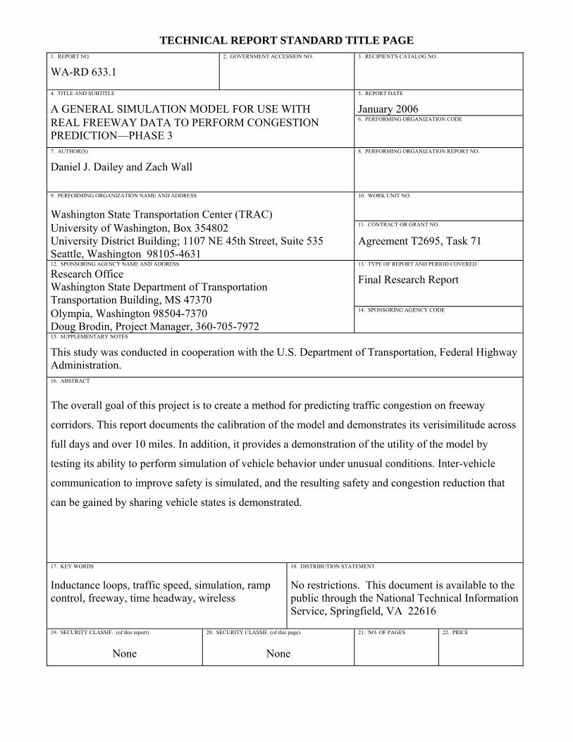
TECHNICAL REPORT STANDARD TITLE PAGE

1. REPORT NO. 2. GOVERNMENT ACCESSION NO. 3. RECIPIENT'S CATALOG NO.

WA-RD 633.1

4. TITLE AND SUBTITLE 5. REPORT DATE

A GENERAL SIMULATION MODEL FOR USE WITH January 2006 REAL FREEWAY DATA TO PERFORM CONGESTION 6. PERFORMING ORGANIZATION CODE PREDICTION—PHASE 3 7. AUTHOR(S) 8. PERFORMING ORGANIZATION REPORT NO.

Daniel J. Dailey and Zach Wall

9. PERFORMING ORGANIZATION NAME AND ADDRESS 10. WORK UNIT NO.

Washington State Transportation Center (TRAC) University of Washington, Box 354802 11. CONTRACT OR GRANT NO.

University District Building; 1107 NE 45th Street, Suite 535 Agreement T2695, Task 71 Seattle, Washington 98105-4631 12. SPONSORING AGENCY NAME AND ADDRESS 13. TYPE OF REPORT AND PERIOD COVERED

Research Office Final Research Report Washington State Department of Transportation Transportation Building, MS 47370

Olympia, Washington 98504-7370 14. SPONSORING AGENCY CODE

Doug Brodin, Project Manager, 360-705-7972 15. SUPPLEMENTARY NOTES

This study was conducted in cooperation with the U.S. Department of Transportation, Federal Highway Administration. 16. ABSTRACT

The overall goal of this project is to create a method for predicting traffic congestion on freeway

corridors. This report documents the calibration of the model and demonstrates its verisimilitude across

full days and over 10 miles. In addition, it provides a demonstration of the utility of the model by

testing its ability to perform simulation of vehicle behavior under unusual conditions. Inter-vehicle

communication to improve safety is simulated, and the resulting safety and congestion reduction that

can be gained by sharing vehicle states is demonstrated.

17. KEY WORDS 18. DISTRIBUTION STATEMENT

Inductance loops, traffic speed, simulation, ramp control, freeway, time headway, wireless

No restrictions. This document is available to the public through the National Technical Information Service, Springfield, VA 22616

19. SECURITY CLASSIF. (of this report) 20. SECURITY CLASSIF. (of this page) 21. NO. OF PAGES 22. PRICE

None None

DISCLAIMER

The contents of this report reflect the views of the authors, who are responsible

for the facts and accuracy of the data presented herein. The contents do not necessarily

reflect the official views or policies of the Washington State Transportation Commission,

Department of Transportation, or the Federal Highway Administration. This report does

not constitute a standard, specification, or regulation.

iii

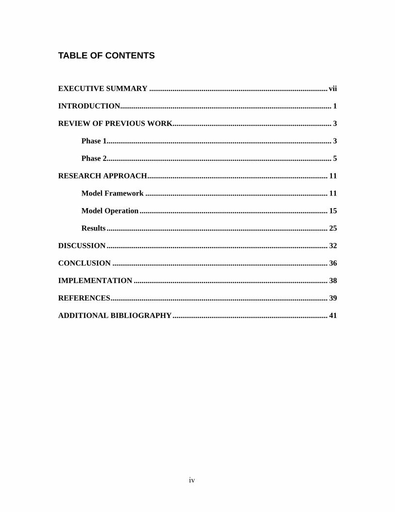
TABLE OF CONTENTS

EXECUTIVE SUMMARY ............................................................................................ vii

INTRODUCTION............................................................................................................. 1

REVIEW OF PREVIOUS WORK.................................................................................. 3

Phase 1.................................................................................................................... 3

Phase 2.................................................................................................................... 5

RESEARCH APPROACH............................................................................................. 11

Model Framework .............................................................................................. 11

Model Operation ................................................................................................. 15

Results .................................................................................................................. 25

DISCUSSION .................................................................................................................. 32

CONCLUSION ............................................................................................................... 36

IMPLEMENTATION .................................................................................................... 38

REFERENCES................................................................................................................ 39

ADDITIONAL BIBLIOGRAPHY................................................................................ 41

iv

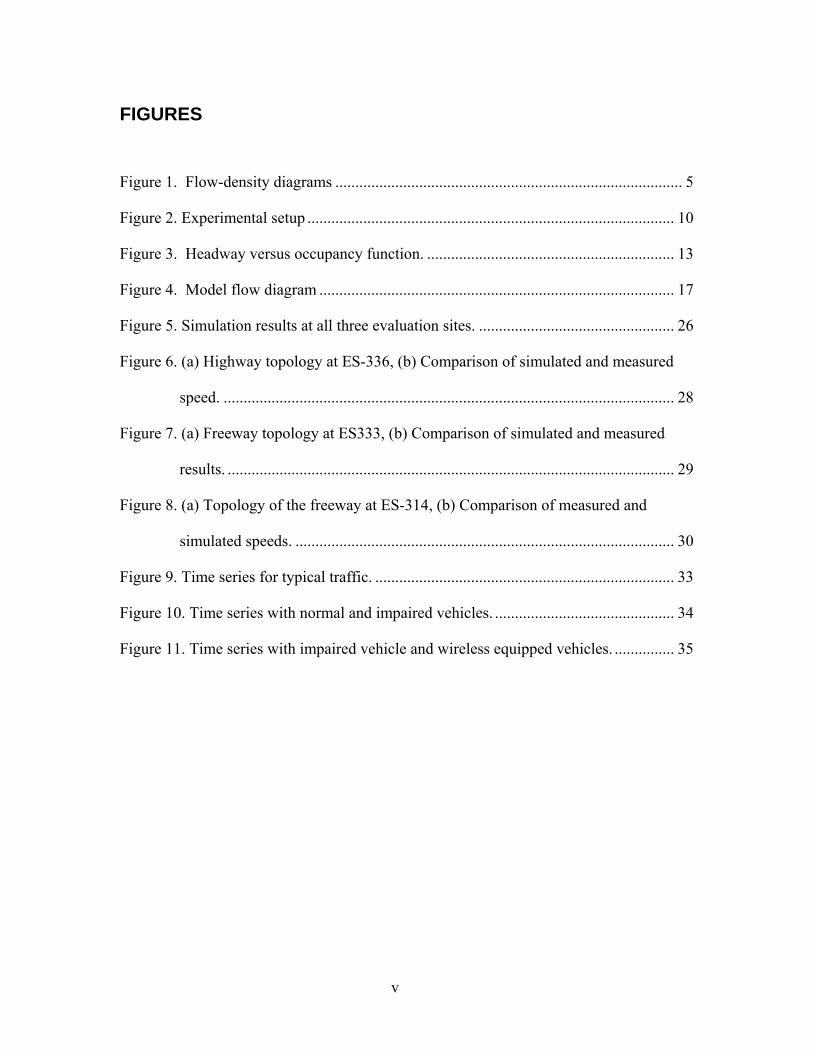
FIGURES

Figure 1. Flow-density diagrams ....................................................................................... 5

Figure 2. Experimental setup ............................................................................................ 10

Figure 3. Headway versus occupancy function. .............................................................. 13

Figure 4. Model flow diagram ......................................................................................... 17

Figure 5. Simulation results at all three evaluation sites. ................................................. 26

Figure 6. (a) Highway topology at ES-336, (b) Comparison of simulated and measured

speed. ................................................................................................................. 28

Figure 7. (a) Freeway topology at ES333, (b) Comparison of simulated and measured

results. ................................................................................................................ 29

Figure 8. (a) Topology of the freeway at ES-314, (b) Comparison of measured and

simulated speeds. ............................................................................................... 30

Figure 9. Time series for typical traffic. ........................................................................... 33

Figure 10. Time series with normal and impaired vehicles. ............................................. 34

Figure 11. Time series with impaired vehicle and wireless equipped vehicles. ............... 35

v

TABLES

Table 1. Acceleration values............................................................................................ 19

vi

EXECUTIVE SUMMARY

The overall goal of this ongoing project is to create a method for predicting traffic

congestion on freeway corridors. Creating a model that accurately replicates and predicts

traffic slowing behavior, and even reverse shock waves, on the basis of congestion is a

difficult and challenging task. In support of this assertion, very few publications exist

that compare model predictions to real, observed traffic speed data over long distances

and across a full day. Ideally, a fully implemented operational model will provide a

traffic service, like that of “pin point Doppler” weather radar, that can predict growing or

dissipating congestion. Furthermore, an operational model can be used to simulate

traffic behavior under a variety of unusual conditions, which in turn allows for the

simulation of the incorporation of new technologies, such as HOT Lanes and inter-

vehicle communication for safety. A student is presently working on the possibility of

improving ramp control by using a “simulator in the loop” framework for global ramp

control.

In the first phase of this project a preliminary version of the model used real-time

loop data to successfully reproduce traffic behavior under moderately congested

conditions. To improve the model for heavily congested conditions, it had to be

accurately calibrated. The process of calibrating the model revealed that inductance loop

errors were preventing accurate results. Therefore, the second phase of this project

focused on developing an algorithm to correct data reported from improperly functioning

loops, which was published at the 2003 Transportation Research Board Annual Meeting.

In this third phase of the project, the corrected loop data from the TDAD (Traffic Data

Acquisition and Distribution) data mine were used to calibrate the model. The algorithm

vii

created in support of this effort can be used with malfunctioning loops to improve the

freeway management system performance monitoring effort.

When run as a simulator, the model can predict recurring congestion, non-

recurring congestion once an incident has been identified and located, and dissipation of

congestion. It can also estimate the effects of lane and road closures on freeway

congestion. When completely implemented, the model will predict 20 to30 minutes into

the future, allowing for improvements in global traffic control strategies such as global

ramp metering. It can also simulate lane closure decisions, as well as predictions useful

for traveler information akin to weather report predictions.

This report documents the Phase 3 calibration of the model and demonstrates its

operation across full days and over 10 miles. In the simulation presented in this report,

the upstream and middle stations did not show a significant level of congestion, and the

downstream station showed the presence of a large amount of congestion. This

congestion was the result of a shockwave propagating back from the downstream

bottleneck. The simulation correctly modeled the onset of the congestion, the entire

congested period, and the dispersal of the congestion. The ability to correctly model these

three periods is a crucial characteristic for a simulator that is designed to be used as part

of a controller. Given that the input to the model is such a long distance from the

congested region, the model can predict congestion at the end approximately 10 minutes

(the approximate travel time from the beginning to the congestion region) before it

actually happens. By using this prediction, a global controller may be better able to adjust

ramp metering rates to reduce the amount of congestion in the system.

As a demonstration of the utility of the model, a simulation to evaluate the

effectiveness of using inter-vehicle communication to improve the safety performance of

viii

the roadway is included in this report. This provides a demonstration of the utility of the

model by testing its ability to perform simulation of vehicle behavior under unusual

conditions. The simulation tested the effectiveness of reducing reaction time by using

inter-vehicle communication when “impaired” vehicles are inserted in the flow. An

initial calibration of the model on SR167 was created, and then an “impaired” vehicle

was inserted into the model. The model showed that the insertion of the “impaired”

vehicle had the potential to reduce traffic speeds by over 10 MPH, and the literature

indicates that a speed reduction of 10 MPH or more is correlated with accidents. The test

simulated vehicles sharing vehicle state via wireless communication by reducing the

reaction time of the driver. When the reaction time was reduced, the speed reduction was

mitigated. Inter-vehicle communication to improve safety was thus simulated, and the

resulting safety and congestion reduction that could be gained by sharing vehicle states

was demonstrated.

At this writing a student is implementing a global “simulator in the loop” ramp

control algorithm that uses the model to predict 15 minutes into the future and estimate

ramp flow rates that will mitigate the start of the shock wave phenomena. This use of

“simulator in the loop” will be compared to the existing localized control to demonstrate

improvements that can be made by using global control. Roadway data from the TDAD

data mine will be used in the validation.

This project developed modeling capabilities at the University of Washington that

can simulate the application of new technologies, geometric changes to the roadway,

and—potentially—global ramp control.

ix

.

x

INTRODUCTION

Simulations are often used to model physical systems that cannot be described by

using an analytical model. In the area of traffic simulation, a number of different models

(and their respective simulators) have been developed for use in the evaluation of many

intelligent transportation systems (ITS) applications—(1) traffic management systems,

(2) traffic control schemes, (3) automated vehicle routing—as well as for planning

purposes. The capabilities of a traffic simulator vary depending upon the task at hand;

certain models are used for planning, while others are incorporated inside advanced

traffic management systems (ATMS). This report presents a traffic model that allows for

accurate traffic flow predictions based on a micro-simulation, making it suitable for

“simulator in the loop” ramp control.

The basic premise of traffic flow modeling is that the evolution of traffic

phenomena can be modeled by using the behavior of the driver [Daganzo 2002]. Whether

drivers are modeled macroscopically or microscopically, these traffic simulators use

quantities such as volume, occupancy, and speed to describe roadway conditions. The

primary purpose of this model is to predict real-time traffic conditions for use in a ramp

control system. The model needs to present an accurate picture of the roadway at a level

that makes sense for traffic control. The existing inductance loop sensor system records

data in 20-second time periods [Dailey et al. 2002]. However, traffic data are quite

variable, given both traffic behavior and sensor noise over such a short time interval. To

filter the high frequency components of the variability, this research used a 5-minute

average as the basic time step for displaying results.

1

Traffic conditions can be expressed by using a number of different quantities:

speed, density, volume, and travel time. Since each quantity captures a different aspect of

traffic, no one variable is sufficient to fully quantify the state of the system. Moreover,

the non-stationary nature of traffic flow means that the transition between states changes

with time. Given the difficulty of predicting traffic behavior, in this effort the focus was

on conservation of cars. In other words, a vehicle added to the model should stay in the

model until it exits the model via a ramp or drives the length of the model.

The literature acknowledges that it is not a trivial task to accurately calculate

conditions of the roadway in between sensors [Krishnamurthy and Coifman 2004]. And

so, creating a traffic model that successfully maintains conservation of cars, while

matching observed conditions, is an important first step in providing a more accurate

calculation of roadway conditions.

2

REVIEW OF PREVIOUS WORK

The work presented herein relies on two past efforts. Phase 1 was an initial

modeling effort for uncongested roadways, and Phase 2 was a data correction effort made

necessary by the nature of the available inductance loop data.

Phase 1

The report from the first phase of this project, A Cellular Automata Model for Use

with Real Freeway Data (WA-RD 537.1), presented a cellular automata model for traffic

flow simulation and prediction (CATS). Cellular automata models quantize complex

behavior into simple individual components. In this model, the freeway being simulated

is discretized into homogeneous cells of equal length, and time is discretized into time-

steps of equal duration. These cells can be either in an occupied or empty state,

depending on whether a vehicle is present at that location. The state of the cells is

updated sequentially at each time step with a set of vehicle position update rules and real-

time volume data sampled from embedded inductance loop traffic sensors on the access

and exit ramps of the freeway. These volume data are used to determine the number of

vehicles entering and exiting the freeway at each time-step. The vehicle position update

rules apply to vehicles already on the freeway. These rules include a car-following,

optimal-headway model, a model for speeding, a model for breaking, a model for lane

changing, and a model for the upstream effects of access and exit ramps. Each of these

motion models has a set of input parameters that governs its behavior. These parameters

can be adjusted to improve the performance of the simulation model. The CATS model

also allows users to define locations within the road topology where volume and density

data will be calculated so that the model results can be compared to observed highway

3

data. These locations usually correspond to the positions of the embedded loop traffic

sensors.

To observe the results of the CATS model when it was used to simulate real

traffic, a case study was conducted on an 11-mile section of the I-5 freeway in Seattle

over a 12-hour period. The actual traffic data provided by the embedded inductance loop

traffic sensors on the freeway and the model were compared by using both qualitative and

quantitative measures. These included statistical conservation and correlation metrics and

comparison of traffic flow versus density plots.

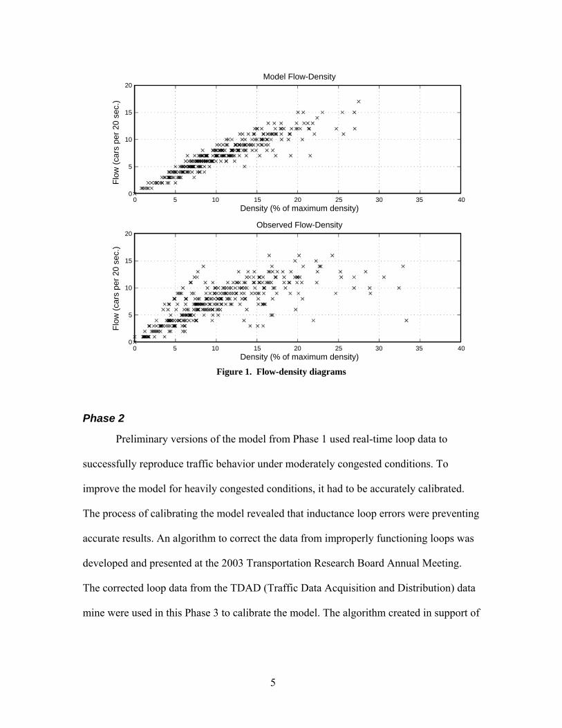
One means of evaluating the model developed in Phase 1 is comparing the

resulting flow-density diagrams. Figure 1 shows the flow-density diagrams for both the

model and the historical data over the same 2-hour period. The similarity between the

two diagrams suggests that the level of congestion of the model matched the level of

congestion on the actual roadway during the test period.

In general, the exit volumes predicted by the model correlated to the volumes of

cars recorded by the sensors. Moreover, the volumes and congestion levels found in the

model were similar to the historical volumes and congestions.

4

Model Flow-Density

Density (% of maximum density)

Observed Flow-Density

Density (% of maximum density)

Flow

(car

s pe

r 20

sec.

)Fl

ow (c

ars

per 2

0 se

c.)

20

15�

10�

5�

0

20

15�

10�

5�

0

0� 5� 10� 15� 20� 25� 30� 35� 40

0� 5� 10� 15� 20� 25� 30� 35� 40

Figure 1. Flow-density diagrams

Phase 2

Preliminary versions of the model from Phase 1 used real-time loop data to

successfully reproduce traffic behavior under moderately congested conditions. To

improve the model for heavily congested conditions, it had to be accurately calibrated.

The process of calibrating the model revealed that inductance loop errors were preventing

accurate results. An algorithm to correct the data from improperly functioning loops was

developed and presented at the 2003 Transportation Research Board Annual Meeting.

The corrected loop data from the TDAD (Traffic Data Acquisition and Distribution) data

mine were used in this Phase 3 to calibrate the model. The algorithm created in support of

5

this effort can be used with malfunctioning loops to improve the freeway management

system performance monitoring effort.

A basic problem with archived data is that invalid data affect the conclusions that

are drawn from them [Brockfield et al. 2005]. Off-line processing of archived data is a

necessary step in any analysis that uses historical records of traffic data. While a number

of authors have proposed methods for determining the validity of sensor data [Brockfield

et al. 2005, Brackstone and McDonald 2003, Winsum and Heino 1996], these methods

are only able to answer the Boolean question of whether the data are good or bad. A

significant problem in the use of loop inductance sensor data is the detection and

recovery of errors that are the result of poorly calibrated sensors. Such sensors generate

data that fall within the hard limits used for error detection but do not accurately

represent the road conditions, and as an important segment of the sensor population, they

need to be explicitly handled.

The problem of adjusting the output of poorly calibrated sensors has previously

been discussed in situations involving dual loop detectors. Ahmed [1999], compared

dual loop “on-time” to identify failed detectors, and Ayres et al. [2001] used an estimate

of vehicle length from paired detectors to identify a set of detector errors.

However, single loop detectors provide the most coverage of the freeway

network and are also prone to calibration errors. Recent work has also used single loops

to correct errors in freeway data [TRB 2000, Bham and Benekohal 2004]. However, these

methods are designed to work with a single loop sensor, while the method presented here

works with pairs of single loop sensors. Poor calibration can result in a loop sensor that

chronically under-counts the traffic passing over it or that chronically over-counts by

counting traffic in neighboring lanes [Kyongsu et al. 2000].

6

Phase 2 produced an algorithm for correcting errors in archived loop data from

the freeway traffic management system that are the result of poorly calibrated sensors.

These errors pose a significant difficulty when archived data are used in off-line analysis

because the calibration errors are difficult to detect with traditional methods. In the work

presented, consistency of vehicle counts is used to judge the validity of the data. That is,

if vehicle counts are balanced, the data are valid; if vehicle counts are not balanced, the

data are not valid. The method also can determine a correction factor. This correction

factor is used to create a time series that can be combined with the original data to adjust

the volume to create a consistent data set.

During the analysis of archival loop sensor data, it is desirable to post-process the

data to detect and recover errors that were not detected when the data were originally

collected. Specifically, the goal of the work in Phase 2 was to recover errors that were the

result of improperly calibrated loops that under/over-counted traffic volumes. During the

development of a simulation model using traffic data, the lack of consistency due to

over/under-counting at various stations posed a significant problem in the development

process. The Phase 2 report presents a method for detecting stations (groups of loop

sensors that span all the lanes of the roadway) that are under/over-counting cars and then

a companion method for recovering the data, essentially balancing the vehicle count at

each station. This method is suitable for creating a valid dataset where vehicle counts are

consistent over a series of stations.

The correction algorithm consists of three basic steps:

1. The first step is to find a reference station that is correctly calibrated, i.e., all

loops are properly counting cars.

7

2. Next, stations adjacent to the reference station are compared to the reference

station. The comparison process determines the validity of the adjacent

station. Either the station is operating correctly, at which point it can be used

as a reference station for another comparison, or errors are present.

3. If errors are present, the bias in the station is calculated, and a correction time

series is applied to the station data.

After correction, the station is then used as the reference station for the next adjacent

station calibration.

The first step in the error correction process is to find a station that is properly

calibrated. Because the error correction algorithm assumes that one station is outputting

correct values, a station must be designated as the ‘reference’ station before the algorithm

can be applied to other stations. To accomplish this, the algorithm searches for two

adjacent stations that are calibrated correctly.

The basic assumption used by this search is that it is possible to reconcile the

vehicle counts in the station data so that the volumes of vehicles entering and exiting the

freeway are consistent with the number of vehicles remaining on the freeway. The same

number of cars counted by the upstream sensor should be counted by the downstream

sensor at some future point in time.

The first step in the process of choosing a reference station is to determine which

stations are potential candidates. The reference station candidates are limited to pairs of

stations that have no on- or off-ramps between the mainline sensor locations.

Given a set of candidates, the next step is to evaluate the historical data quality of

the sensors by using the error algorithms built into the sensors. The number of samples

recorded over a 24-hour period is divided by the total number of 20-second intervals in

8

that period to verify that the loop detector is functioning continuously, and this fraction is

used as a quantitative measure of data completeness. The ratio of the number of samples

identified as valid (by the error algorithms built into the sensors) to the total number of

observed samples is used as quantitative measure of the data validity. The multiple of

these two measures is used as a likelihood measure, and sensors with less than a 95

percent likelihood are removed from consideration as a reference station.

Finally, the station pairs that meet the first two criteria are evaluated to determine

the cumulative deviation in volume count over a 24-hour period for 30 different days.

Using the earlier calculation of the lag between the two sensors, the total volume of cars

counted by the upstream station is compared to the total volume of cars counted by the

downstream station.

To compare the target station with the reference station, the time lag between the

two stations must be determined. This time lag is required to account for the time a

vehicle takes to travel between the two stations. Unlike dual loop sensor configurations,

where the loop sensors are typically less than 15 meters apart, the distance between two

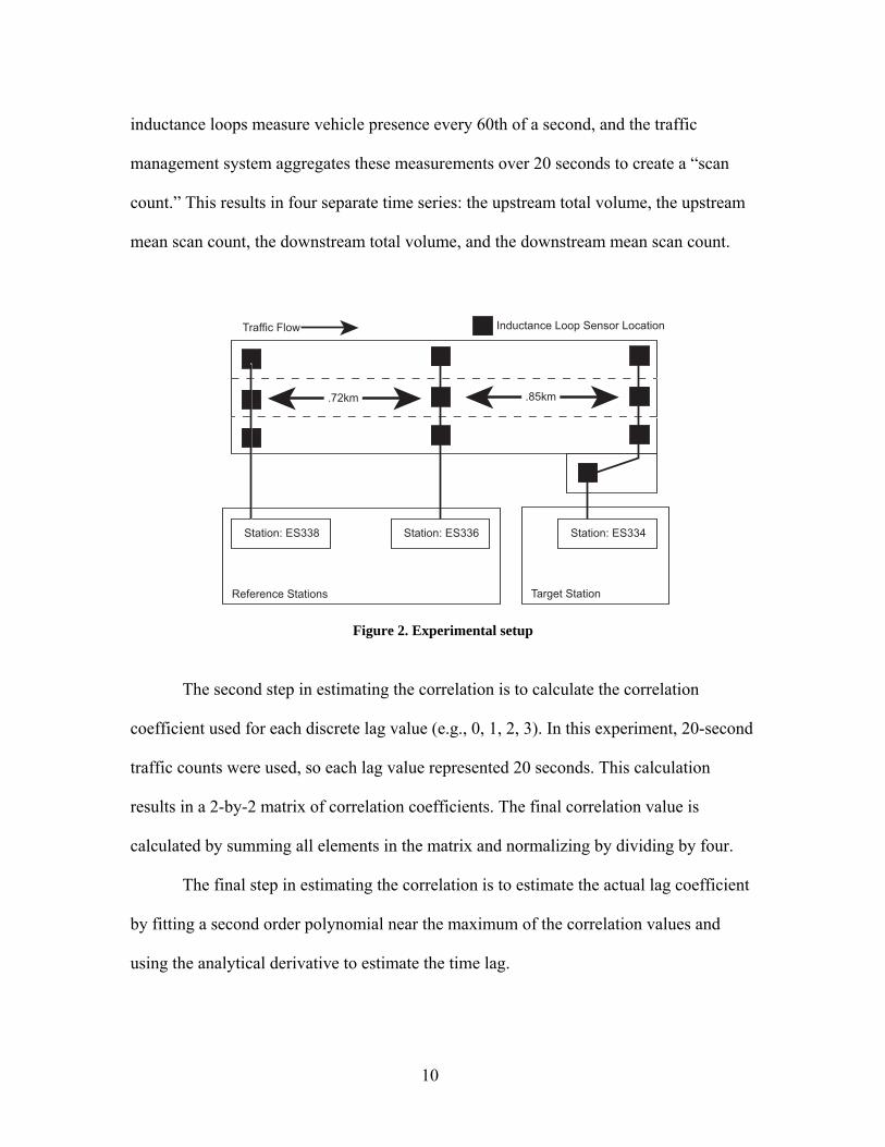
single loop sensors is much larger. In the Phase 2 experiment, the stations were .72km to

.90km apart. Figure 2 shows the basic configuration of the sensors used in the

experiment. The data used in the experiment were collected from SR 167 in Washington

State over a series of Wednesdays in 2000 and 2001 when no incidents occurred. The

time lag (τ) is calculated by finding the value that results in the largest correlation

coefficient when the output of the two stations is compared.

The correlation coefficient between the two stations is calculated in three steps.

The first step is to aggregate the loop data. To do this, the total volume at each time step

across all lanes for both the target and reference stations is computed. In addition, the

9

inductance loops measure vehicle presence every 60th of a second, and the traffic

management system aggregates these measurements over 20 seconds to create a “scan

count.” This results in four separate time series: the upstream total volume, the upstream

mean scan count, the downstream total volume, and the downstream mean scan count.

Target Station

Inductance Loop Sensor Location

Station: ES338

.72km .85km

Station: ES336 Station: ES334

Traffic Flow

Reference Stations

Figure 2. Experimental setup

The second step in estimating the correlation is to calculate the correlation

coefficient used for each discrete lag value (e.g., 0, 1, 2, 3). In this experiment, 20-second

traffic counts were used, so each lag value represented 20 seconds. This calculation

results in a 2-by-2 matrix of correlation coefficients. The final correlation value is

calculated by summing all elements in the matrix and normalizing by dividing by four.

The final step in estimating the correlation is to estimate the actual lag coefficient

by fitting a second order polynomial near the maximum of the correlation values and

using the analytical derivative to estimate the time lag.

10

RESEARCH APPROACH

Phase 3 of this effort created a model that can accurately simulate the propagation

of vehicles over 10 miles and through the course of an entire day. The bases for the

model are conservation of vehicles and new insights involving the time headway between

vehicles. These two ideas are combined with an optimal controller model from an

advanced cruise control to propagate the vehicle through the model.

Model Framework

To enforce the conservation of cars in the model, several specific roadway

sensors—the sensors that monitor locations at the edges of our model—are assumed to

have an exact count of the vehicles that are entering or leaving the roadway. As such, if

the sensor reports that 10 vehicles passed the entry point in a particular time step, then 10

vehicles are added into the model at the corresponding time step. By using this

assumption, the model will have an accurate representation of the vehicles that are on the

roadway.

Beyond the conservation of cars, the other foundation for the model is driver

headway. A basic parameter in any microscopic simulation, the headway that drivers

maintain between their car and the car in front of them is a very predictive aspect of a

driver’s behavior [Brockfield et al. 2005]. Driver headway is often modeled by using the

concept of “desired headway,” which is based on the assumption that each driver has a

specific headway that s/he is comfortable driving with and that each driver will adjust the

speed of the vehicle to conform to a particular headway [Brackstone and McDonald

2003]. The process of adjusting speed to maintain this headway because of another

vehicle being within the perception range of the driver is called “car following.” The

11

process of adjusting speed when there is not another vehicle within the perception range

is called “free-flow driving.” A driver’s headway is a very important parameter in a

microscopic model, both because it governs behavior during car following and helps

determine when the car moves between car following and free-flow driving modes.

Headway is represented in terms of either the distance between two cars, termed

space headway, or the time between two cars, called time headway. Previous research has

shown that drivers often maintain a constant time headway and adjust the distance

between the vehicles on the basis of their current speed [Winsum and Heino 1996]. Given

this result, existing microscopic models typically assign vehicles in the model a time

headway that is used for all car following calculations—often from a distribution in order

to model the behavior of different types of drivers (aggressive, defensive, etc.) [Bham

and Benekohal 2004]. However, new research has shown that drivers will adjust their

headway on the basis of traffic conditions. The end result is that time headway does not

vary with speed; it varies with traffic conditions [Ayres et al. 2001].

To create a model of driver time headways that works with a real-time data input,

an empirical lookup table was created to provide an estimate of the average time headway

from real-time data. Loop sensors sample at a frequency of 60 Hz and return average

results for each 20-second time period. The recorded data are the number of vehicles that

passed during that period, as well as the number of samples that registered as having a

vehicle present over the loop. From this, the average headway of the vehicles that pass

during a particular 20-second period is calculated:

( )k

kk volume

countscanheadwayaverage

⋅−

=60

_1200_

Eq. 1

12

where volumek is the number of vehicles that crossed at timestep k

scan_countk is the number of high samples at timestep k.

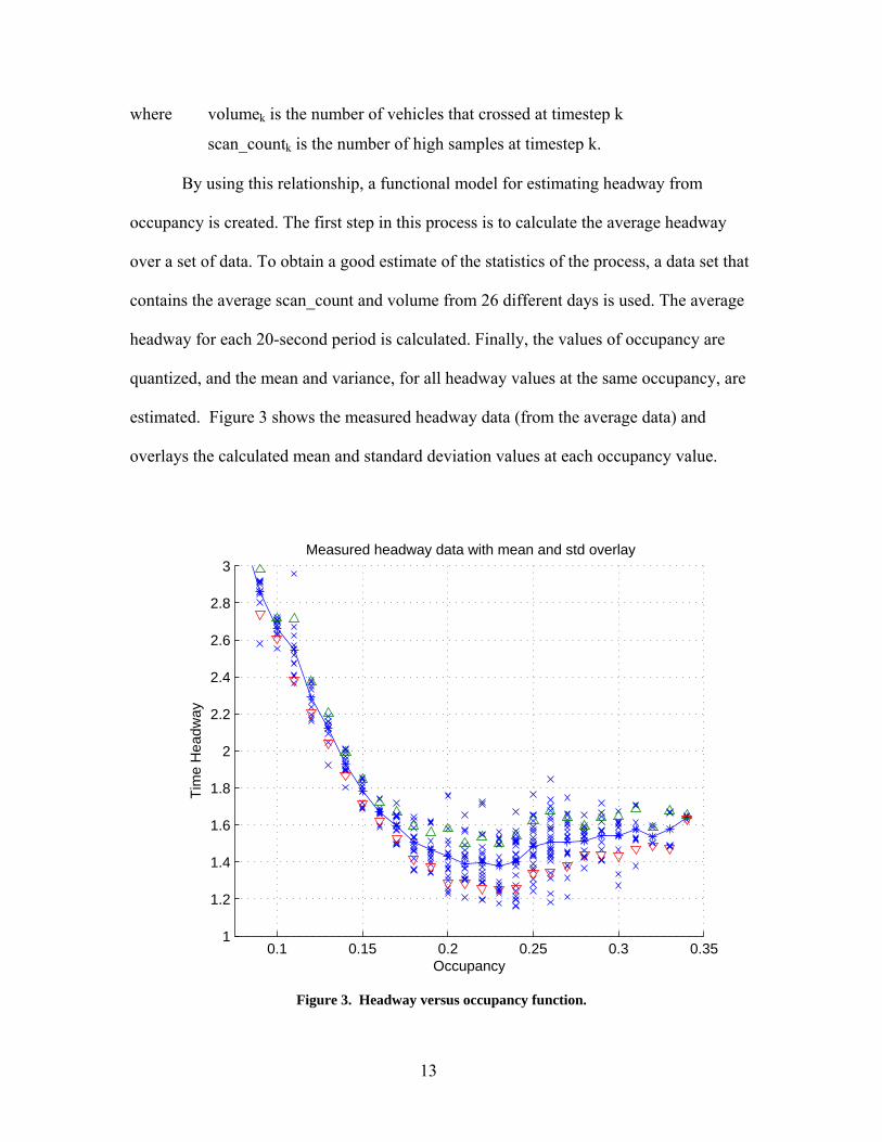
By using this relationship, a functional model for estimating headway from

occupancy is created. The first step in this process is to calculate the average headway

over a set of data. To obtain a good estimate of the statistics of the process, a data set that

contains the average scan_count and volume from 26 different days is used. The average

headway for each 20-second period is calculated. Finally, the values of occupancy are

quantized, and the mean and variance, for all headway values at the same occupancy, are

estimated. Figure 3 shows the measured headway data (from the average data) and

overlays the calculated mean and standard deviation values at each occupancy value.

0.1 0.15 0.2 0.25 0.3 0.351

1.2

1.4

1.6

1.8

2

2.2

2.4

2.6

2.8

3

Occupancy

Tim

e H

eadw

ay

Measured headway data with mean and std overlay

Figure 3. Headway versus occupancy function.

13

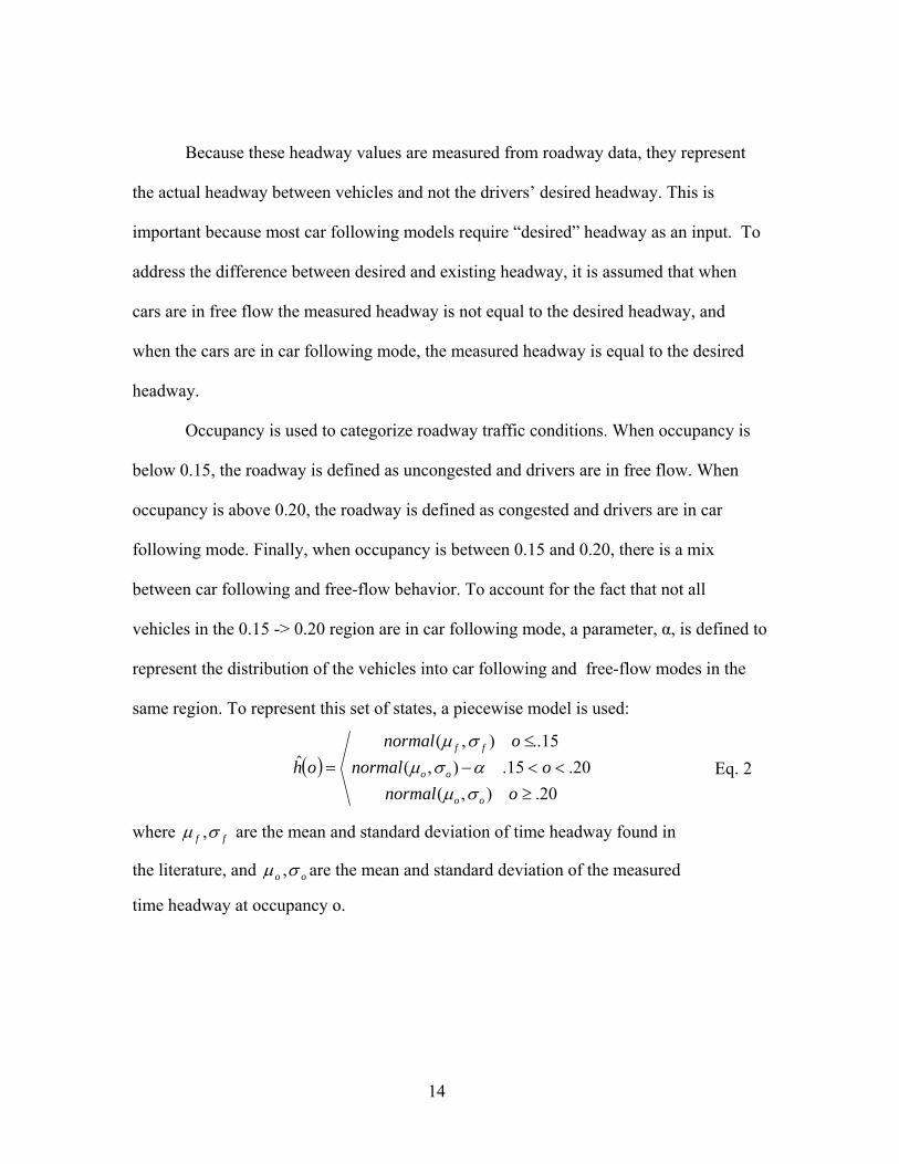
Because these headway values are measured from roadway data, they represent

the actual headway between vehicles and not the drivers’ desired headway. This is

important because most car following models require “desired” headway as an input. To

address the difference between desired and existing headway, it is assumed that when

cars are in free flow the measured headway is not equal to the desired headway, and

when the cars are in car following mode, the measured headway is equal to the desired

headway.

Occupancy is used to categorize roadway traffic conditions. When occupancy is

below 0.15, the roadway is defined as uncongested and drivers are in free flow. When

occupancy is above 0.20, the roadway is defined as congested and drivers are in car

following mode. Finally, when occupancy is between 0.15 and 0.20, there is a mix

between car following and free-flow behavior. To account for the fact that not all

vehicles in the 0.15 -> 0.20 region are in car following mode, a parameter, α, is defined to

represent the distribution of the vehicles into car following and free-flow modes in the

same region. To represent this set of states, a piecewise model is used:

( )20.),(

20.15.),(15..),(

ˆ

≥<<−

≤=

onormalonormal

onormaloh

oo

oo

ff

σμασμ

σμ Eq. 2

where ff σμ , are the mean and standard deviation of time headway found in

the literature, and oo σμ , are the mean and standard deviation of the measured

time headway at occupancy o.

14

Model Operation

The headway-based, multiple flow state framework described above is used as

part of the model update function. For each vehicle, the local occupancy is calculated and

a new headway is calculated. If the new headway is significantly different from the

current headway, the headway is updated, and a new set of driver control parameters is

generated.

Once the cars have been added to the model, the next step is to move them. To

keep the model simple, each lane is modeled as a first in/first out (FIFO) list of cars. The

first car in the list is the car that is farthest downstream, and the last car in the list is the

car that was most recently added. By iterating down the list (from the first car to the last),

the flow of cars downstream is simulated. At the beginning of each time step, a

“snapshot” of the roadway conditions is saved. These conditions are used to calculate the

“state” of each car, and this state is used to determine acceleration. The three basic state

factors are (1) the distance between the current vehicle and the vehicle in front of it, (2)

the difference in velocity between the current vehicle and the vehicle in front of it, and

(3) the current velocity of the vehicle. Vehicles are moved serially from the farthest

downstream vehicle to the farthest upstream vehicle. Moving the downstream vehicles

first creates the space necessary for the upstream vehicles to fit into.

The update process begins with the first vehicle. Unlike other vehicles in the lane,

the first vehicle does not have a vehicle to follow. As such, the first vehicle is always in

the free-flow state. The update process for the first vehicle is quite simple. The current

speed is compared with the maximum desired speed, and if the current speed is below the

maximum speed, it is increased to the maximum speed.

15

Next, the remaining vehicles in order from downstream to upstream are updated.

The update process is simple, and a functional diagram of the process is shown in Figure

4. First, the model determines which rule to use to determine the vehicle’s acceleration

and calculates the acceleration for the next time step. Second, the model checks the

current occupancy of the local region in front of the vehicle and adjusts the desired

headway on the basis of road conditions. Third, the model checks to see whether the

vehicle is in a position to pass the vehicle in front of it and adjusts the lane as necessary.

Finally, the model checks to see whether the vehicle has tripped any sensors and adjusts

the information as necessary.

Four basic rules are used to determine the acceleration of the current vehicle:

• free-flow braking

• free-flow driving

• car following when the lead vehicle is accelerating

• car following when the lead vehicle is decelerating.

The free-flow braking rule is the only rule that depends on prior state information;

the other three compute the acceleration as a function of the current state of the vehicle.

The main purpose of the free-flow braking routine is to account for situations that

are not handled well by the other rules. One such situation is when a vehicle in free flow

approaches congested traffic. On one hand, the vehicle is in free flow because the vehicle

in front of it is not close enough to follow. However, car following models are structured

around the idea that driver of the following car is trying to maintain a speed similar to

that of the car in front of it. This assumption limits how large of a difference in velocity

between the leader and the follower is possible. Accordingly, if a vehicle traveling 60

mph approaches a vehicle that is traveling 40 mph, the approaching vehicle must slow

16

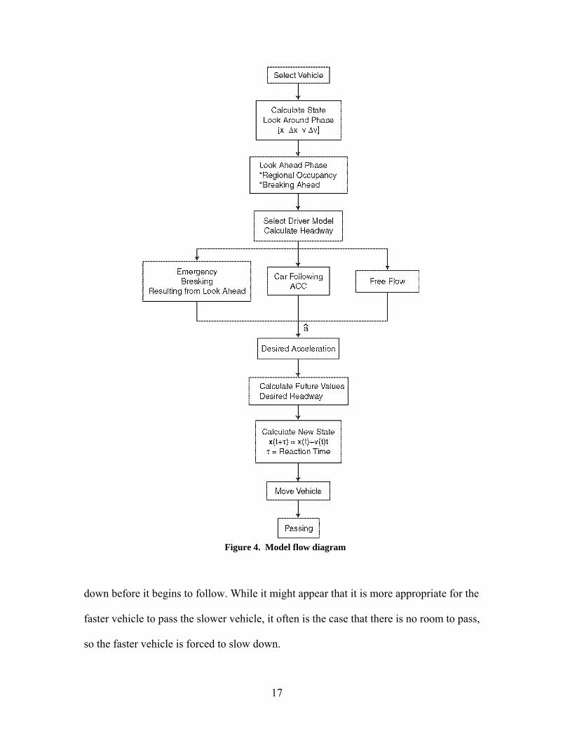
Figure 4. Model flow diagram

down before it begins to follow. While it might appear that it is more appropriate for the

faster vehicle to pass the slower vehicle, it often is the case that there is no room to pass,

so the faster vehicle is forced to slow down.

17

A number of different conditions need to be fulfilled before the free-flow braking

routine is triggered. The two basic conditions are that the vehicle must be in free-flow

(the current headway is greater than the car following headway) and that the distance

between the vehicle and the vehicle in front of it is less than 500 feet. If these conditions

are met, the free-flow braking routine is then triggered if the speed of the leading vehicle

is more than 2 feet/second slower than the approaching vehicle or if the approaching

driver perceives the brake lights of the leading vehicle. The model flags that the driver

perceives brake lights if the leading vehicle has been decelerating for the last four time

steps (2 seconds). If these conditions are met, the free-flow braking routine determines a

constant deceleration that will slow the vehicle down to match the leading vehicle’s

speed in 3 seconds. To account for the fact that most vehicles are not able to instantly

reach their maximum deceleration, an additional check is made to reduce the applied

acceleration if the car was previously accelerating or coasting. The final acceleration is

then passed onto the next stage of the move car routine.

Next, the vehicle is tested to see whether it is in a free-flow driving condition. If

the speed of the vehicle is greater than 50 feet per second and the current time headway is

larger than the vehicle’s specified headway, the acceleration of the vehicle is determined

by using the free-flow driving rules. The rules for free-flow driving are simple. If the

vehicle was previously decelerating, the acceleration is set to zero. Otherwise, the

vehicle’s acceleration is set by using a two regime acceleration model (shown in Table 1)

similar to the one used by Bham and Benekohal [2004].

18

Table 1. Acceleration values

Condition Acceleration

V > 35 mph .8 ft/sec

V < 35 mph 2.4 ft/sec

Abs(V-Vmax) < 1 mph 0 ft/sec

If a vehicle is not in a state of free-flow driving, the model assumes that it is

following the vehicle in front of it. While the model takes into account whether the

leading vehicle is accelerating or decelerating, the actual system used to calculate the

vehicle’s response is the same regardless (only the parameters change). Many types of car

following models have been proposed over the last 50 years. However, the basic

approach for all of them is the same. Namely, the response of the vehicle (its

acceleration) is a function of two things: the current “state” of the vehicle (how fast it is

going, what the distance between it and the leading vehicle is, etc.) and the “stimulus”

that the driver receives (i.e., the difference in velocity between the two vehicles). While

the implementations used can vary widely from model to model, these basic quantities

are always present.

Beyond the current state and stimulation, a car following model must also have a

notion of what the desired state is. All car following models operate under the assumption

that when drivers follow behind other vehicles they are constantly trying to maintain a

balance between them and the driver ahead of them. One common way of describing this

balance is the headway between cars. In our model, the driver adjusts the acceleration of

the car in an effort to maintain this desired headway.

On the basis of concepts from automatic cruise control literature, the controller

was developed by using the framework of a linear quadratic regulator (LQR) controller.

19

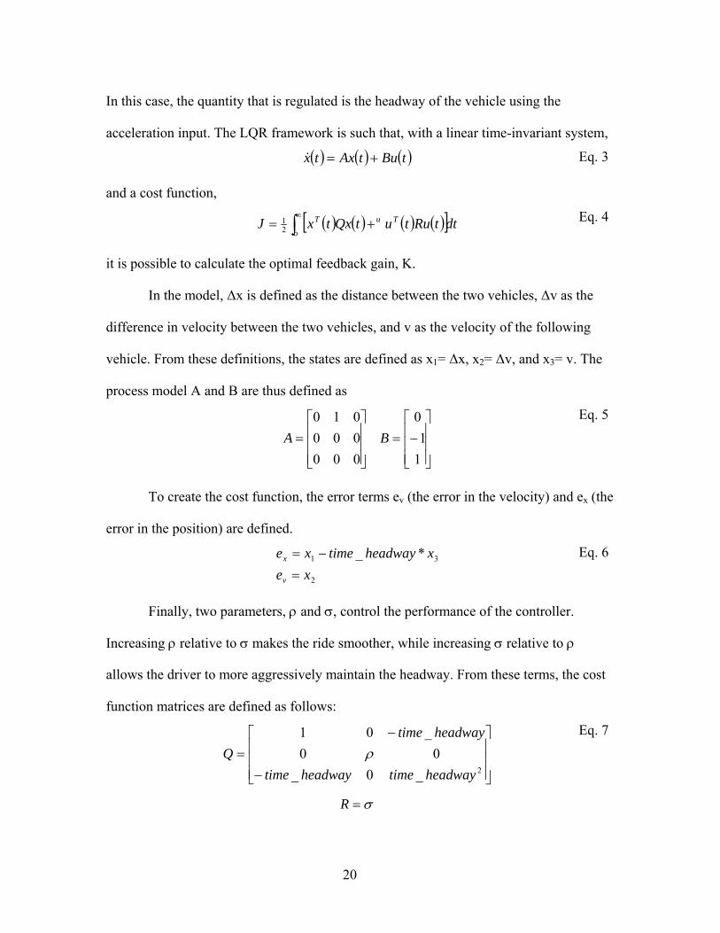
In this case, the quantity that is regulated is the headway of the vehicle using the

acceleration input. The LQR framework is such that, with a linear time-invariant system,

( ) ( ) ( )tButAxtx += Eq. 3

and a cost function,

( ) ( ) ( ) ( )[ ]dttRututQxtxJo

TuT∫∞

+= 21 Eq. 4

it is possible to calculate the optimal feedback gain, K.

In the model, Δx is defined as the distance between the two vehicles, Δv as the

difference in velocity between the two vehicles, and v as the velocity of the following

vehicle. From these definitions, the states are defined as x1= Δx, x2= Δv, and x3= v. The

process model A and B are thus defined as

⎥⎥⎥

⎦

⎤

⎢⎢⎢

⎣

⎡−=

⎥⎥⎥

⎦

⎤

⎢⎢⎢

⎣

⎡=

11

0

000000010

BA

Eq. 5

To create the cost function, the error terms ev (the error in the velocity) and ex (the

error in the position) are defined.

2

31 *_xe

xheadwaytimexe

v

x

=−=

Eq. 6

Finally, two parameters, ρ and σ, control the performance of the controller.

Increasing ρ relative to σ makes the ride smoother, while increasing σ relative to ρ

allows the driver to more aggressively maintain the headway. From these terms, the cost

function matrices are defined as follows:

⎥⎥⎥

⎦

⎤

⎢⎢⎢

⎣

⎡

−

−=

2_0_00

_01

headwaytimeheadwaytime

headwaytimeQ ρ

σ=R

Eq. 7

20

The model at this point is analogous to the automatic cruise control model

developed by Kyongsu et al. [2000]. However, that model is a continuous controller that

is used in an actual car. For the purposes of this effort, a discrete controller that will

function in a simulator is needed. To prepare the controller for use in the simulator, it is

converted from a continuous model to a discrete one by using a zero-order hold on the

inputs and a sample time of .5 seconds [Cleghorn et al. 1991], resulting in the following

model:

⎥⎥⎥

⎦

⎤

⎢⎢⎢

⎣

⎡−

−=

⎥⎥⎥

⎦

⎤

⎢⎢⎢

⎣

⎡=

5.5.

1250.

10001005.1

DD BA

Eq. 8

Values for ρ and σ are needed, and in the literature, a number of researchers have

found that drivers behave differently depending on whether the vehicle in front of them is

accelerating or decelerating relative to them [Jacobson et al. 1990]. This is typically

modeled by having two different sets of parameters, one for the acceleration case and one

for the deceleration case. This approach was adopted, and different values of ρ and σ

were used, depending upon the sign of Δv. These values were adjusted during the model

verification process discussed later. For the results presented in this report, the following

values were used:

Leader Accelerating Leader Decelerating

6010

==

d

d

σρ

10010

==

a

a

σρ

With these parameters, the final values of Q and R to be used by the controller

can be calculated. Given A,B,Q,R, the discrete algebraic Riccati equation

0)( 1 =++−− − QPABPBBRPBAPPAA T

DDT

DDT

DDT

D Eq. 9

21

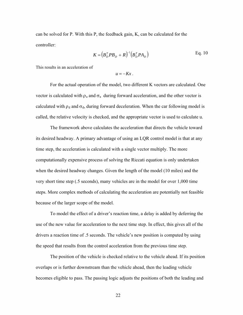
can be solved for P. With this P, the feedback gain, K, can be calculated for the

controller:

( ) ( )DTDD

TD PABRPBBK 1−

+= Eq. 10

This results in an acceleration of Kxu −= .

For the actual operation of the model, two different K vectors are calculated. One

vector is calculated with ρa and σa during forward acceleration, and the other vector is

calculated with ρd and σd, during forward deceleration. When the car following model is

called, the relative velocity is checked, and the appropriate vector is used to calculate u.

The framework above calculates the acceleration that directs the vehicle toward

its desired headway. A primary advantage of using an LQR control model is that at any

time step, the acceleration is calculated with a single vector multiply. The more

computationally expensive process of solving the Riccati equation is only undertaken

when the desired headway changes. Given the length of the model (10 miles) and the

very short time step (.5 seconds), many vehicles are in the model for over 1,000 time

steps. More complex methods of calculating the acceleration are potentially not feasible

because of the larger scope of the model.

To model the effect of a driver’s reaction time, a delay is added by deferring the

use of the new value for acceleration to the next time step. In effect, this gives all of the

drivers a reaction time of .5 seconds. The vehicle’s new position is computed by using

the speed that results from the control acceleration from the previous time step.

The position of the vehicle is checked relative to the vehicle ahead. If its position

overlaps or is further downstream than the vehicle ahead, then the leading vehicle

becomes eligible to pass. The passing logic adjusts the positions of both the leading and

22

the following vehicles to approximate the steady state road conditions after the vehicle

has completed the passing maneuver. The transient effect of passing is not modeled, but

instead, the two vehicles are evenly spread out in the space between the other vehicles in

the lane.

During the process of moving a vehicle, the surrounding traffic conditions are

also measured. To capture local congestion, the occupancy of the five vehicles in front of

the current vehicle is measured. This is calculated by first calculating the amount of time

that each vehicle would occupy a loop sensor:

( )i

ii v

loccupancyvehicle

6_

+=

Eq. 11

where li is the length of vehicle i

vi is the speed of vehicle i

Then occupancy in the region around vehicle i is calculated:

τ

∑= k

k

i

occupancyvehicleoccupancylocal

__

Eq. 12

where τ is the time delta between vehicle i and the sixth vehicle in front of it.

If the local occupancy is above 15 percent, then the model determines whether the

headway should be adjusted. If the current desired headway of the vehicle is outside the

boundary prescribed by the functional relationship between occupancy and headway,

then a new headway is assigned to the vehicle by using the distribution that results from

evaluating the function at the current occupancy. Finally, the controller gain, K, is re-

calculated with the new headway value.

Once all vehicles have been moved, the model does a number of checks to

determine the state of the model: (1) vehicles that have moved beyond the end of the

model are removed, (2) vehicles that have crossed sensors are counted, and (3) vehicles

23

that have exited via off-ramps are also removed. The process of removing vehicles via

off-ramps is a two-stage process. The first step takes place before the vehicles are moved,

and the second step takes place after all the vehicles have been moved.

First, before any vehicles are moved, the model flags off-ramps that are expecting

a vehicle to exit from it. Much like the on-ramp procedure, the sensor data for the off-

ramp are analyzed, and exit times are evenly distributed throughout the time period. For

example, if the 20-second off-ramp data say that 10 vehicles exited via a particular ramp,

the model marks that a vehicle leaves the model via that ramp every four time steps. The

model determines which lane the vehicle exited from by using a historical distribution

and flags the off-ramp.

Second, after all vehicles have been moved, the new position of each vehicle is

checked, and if a vehicle had crossed the off-ramp location during the vehicle movement

process and that off-ramp is flagged, the vehicle is removed and the flag is toggled off. In

the same way as for the on-ramps, only one vehicle is allowed to leave the vehicle via

off-ramps during a single time step. If the model flags an off-ramp to remove a vehicle,

but a vehicle does not cross that off-ramp point, the flag carries over to the next time step.

While it is possible for the demand for removing vehicles to exceed the actual number of

vehicles crossing the off-ramp for an extended period of time, in practice this does not

happen, and the vehicle is removed within one or two time steps (1 second) of when it

was supposed to be removed.

After the removal of vehicles has been handled, the model adds the sensor

information from the current time step to the overall totals. The model keeps track of

volume, occupancy, and speed information in 20-second intervals (40 time steps). The

sensor information is generated in such a way that when the model is working properly,

24

the data the model outputs are the same as the actual measurements from the roadway.

This allows a very straightforward method for validating the model to be used.

Results

With the driver model described above, the traffic performance on a chosen

roadway can be modeled. In this experiment, a 10-mile stretch of Southbound SR 167 in

Washington State was used. Most of the length of the roadway is a two-lane freeway with

a third HOV lane. At approximately the 8.5-mile marker, the HOV restriction is removed.

Shortly after this, the three-lane freeway merges into a two-lane freeway for about a half-

mile stretch. The model simulated the traffic flow over the entire 10-mile stretch of

roadway for a 24-hour period.

The inputs to the model were loop sensor data from sensors located at the

upstream boundary and on-the ramps of the roadway. These included the mainline

individual lane sensors at the upstream location, mile zero, and all of the on- and off-

ramps along the 10-mile stretch. The data used for the validation process were from a

weekday during the summer and were free from the external effects of weather or

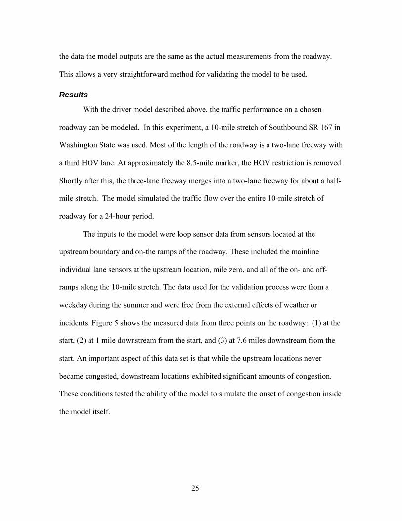
incidents. Figure 5 shows the measured data from three points on the roadway: (1) at the

start, (2) at 1 mile downstream from the start, and (3) at 7.6 miles downstream from the

start. An important aspect of this data set is that while the upstream locations never

became congested, downstream locations exhibited significant amounts of congestion.

These conditions tested the ability of the model to simulate the onset of congestion inside

the model itself.

25

5 10 15 200

10

20

30

40

Time (Hours)

Flo

w (

Veh

icle

s/20

sec

) Flow, station ES−336

5 10 15 200

10

20

30

40

Time (Hours)

Flo

w (

Veh

icle

s/20

sec

) Flow, station ES−333

5 10 15 200

10

20

30

40

Time (Hours)

Flo

w (

Veh

icle

s/20

sec

) Flow, station ES−314

5 10 15 200

20

40

60

Time (Hours)

Spe

ed (

MP

H)

Speed, station ES−336

5 10 15 200

20

40

60

Time (Hours)S

peed

(M

PH

)

Speed, station ES−333

5 10 15 200

20

40

60

Time (Hours)

Spe

ed (

MP

H)

Speed, station ES−314

Figure 5. Simulation results at all three evaluation sites.

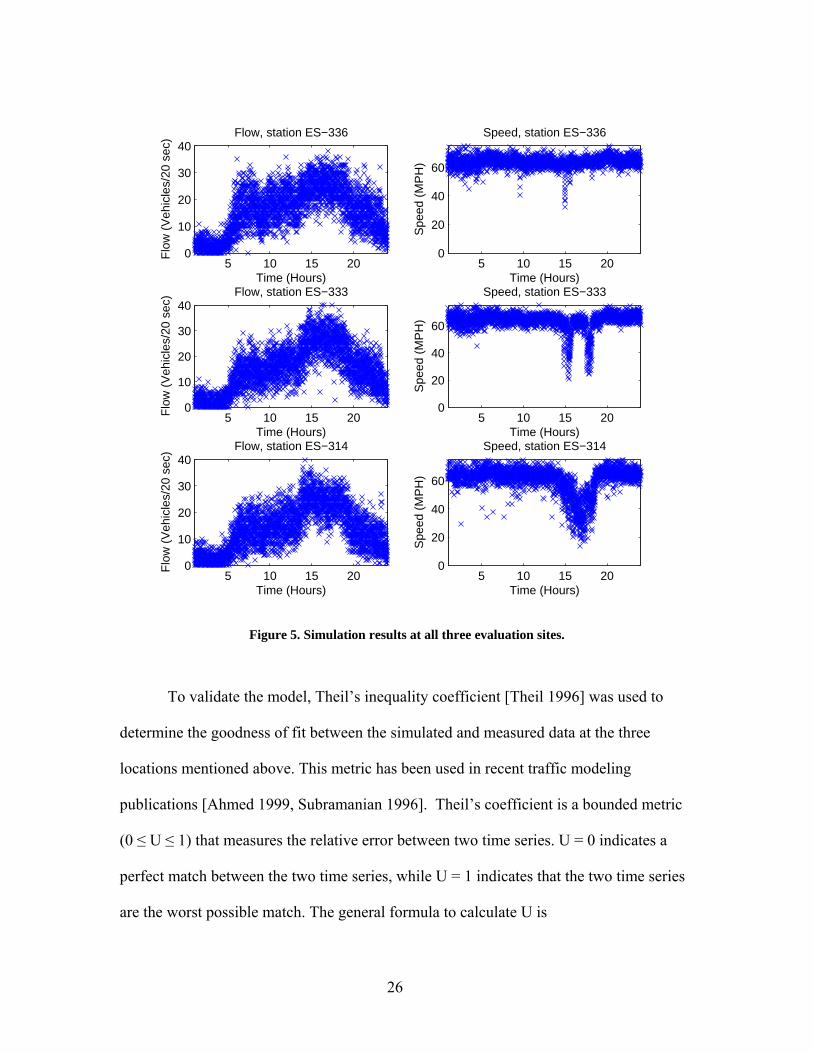
To validate the model, Theil’s inequality coefficient [Theil 1996] was used to

determine the goodness of fit between the simulated and measured data at the three

locations mentioned above. This metric has been used in recent traffic modeling

publications [Ahmed 1999, Subramanian 1996]. Theil’s coefficient is a bounded metric

(0 ≤ U ≤ 1) that measures the relative error between two time series. U = 0 indicates a

perfect match between the two time series, while U = 1 indicates that the two time series

are the worst possible match. The general formula to calculate U is

26

Eq. 13 ( )

( ) ( )∑∑

∑

==

=

+

−=

N

iiN

N

iiN

N

iiiN

xx

xxU

1

21

1

21

1

21

ˆ

ˆ

where is the measured data at time step i ix

ix̂ is the simulated data at time step i

Figure 6a shows the comparison between the measured loop sensor data and the

model at the upstream station, and Figure 6b shows the topology of the roadway. At the

upstream station, Theil’s coefficient was 0.0124. This demonstrates that the method used

to add vehicles into the simulation closely matches the measurements of the inductance

loop sensors. To improve the clarity of the figures, the sensor data were aggregated into

5-minute time averages. However, the calculation of Theil’s coefficient used the 20-

second data.

Figure 7a shows the comparison between the measured loop sensor data and the

model at approximately 1 mile downstream of the start, and Figure 7b shows the

topology of the roadway. At this middle station, Theil’s coefficient was 0.0455. This

result shows that the model was able to simulate the propagation of vehicles down a

relatively short segment of roadway with a high level of fidelity.

Finally, Figure 8a shows the comparison between the measured loop sensor data

and the model at approximately 7.6 miles downstream of the start, and Figure 8b shows

the topology of the roadway. At this downstream station, Theil’s coefficient was 0.0719.

This result shows that the model was able to simulate the propagation of vehicles down a

long segment of roadway while still maintaining a high level of fidelity.

27

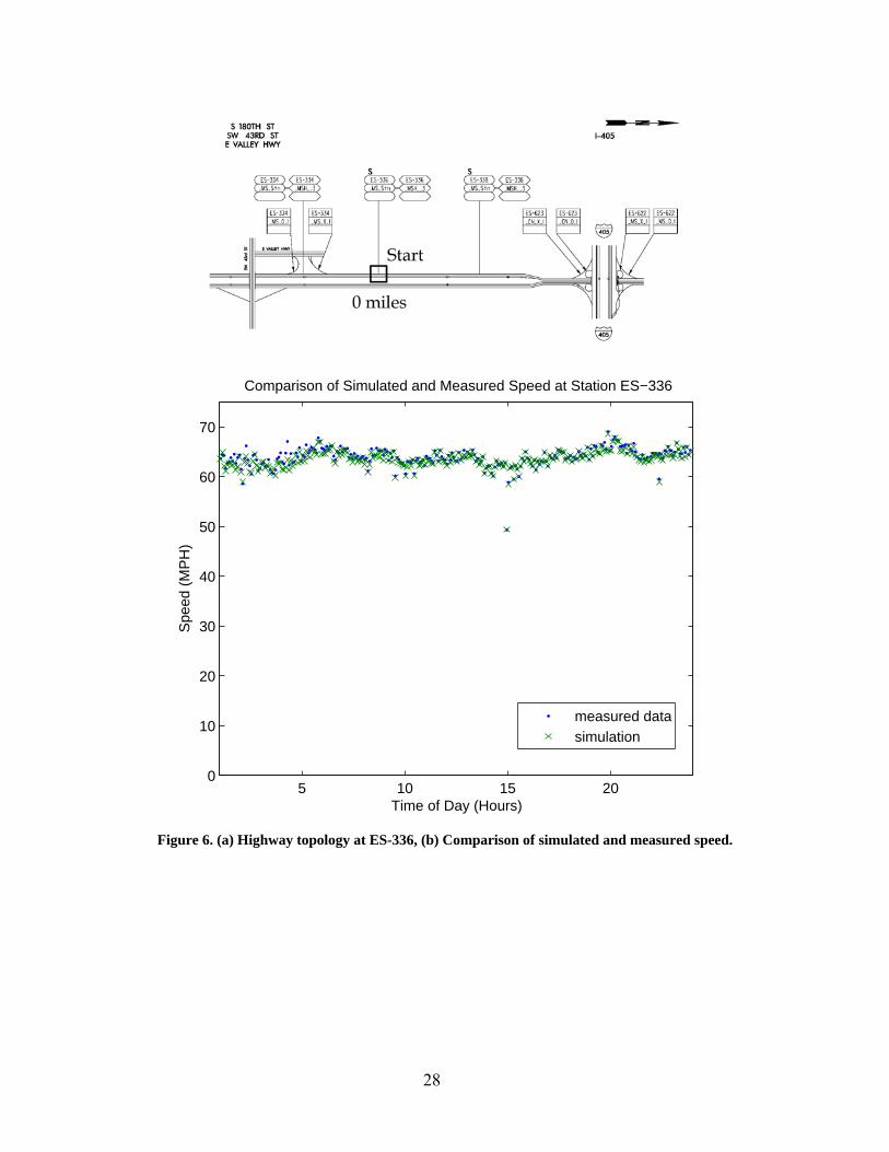
Figure 6. (a) Highway topology at ES-336, (b) Comparison of simulated and measured speed.

5 10 15 200

10

20

30

40

50

60

70

Time of Day (Hours)

Spe

ed (

MP

H)

Comparison of Simulated and Measured Speed at Station ES−336

measured datasimulation

28

Figure 7. (a) Freeway topology at ES333, (b) Comparison of simulated and measured results.

5 10 15 200

10

20

30

40

50

60

70

Time of Day (Hours)

Spe

ed (

MP

H)

Comparison of Simulated and Measured Speed at Station ES−333

measured datasimulation

29

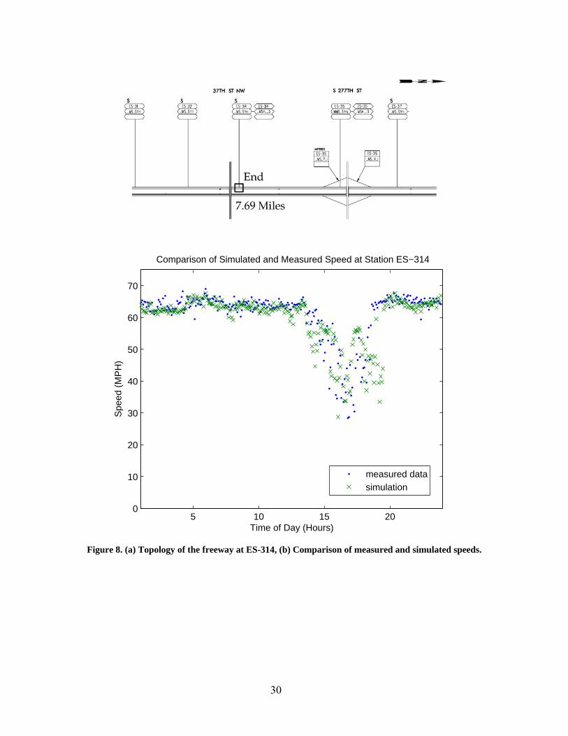
Figure 8. (a) Topology of the freeway at ES-314, (b) Comparison of measured and simulated speeds.

5 10 15 200

10

20

30

40

50

60

70

Time of Day (Hours)

Spe

ed (

MP

H)

Comparison of Simulated and Measured Speed at Station ES−314

measured datasimulation

30

While the upstream and middle stations did not show a significant level of

congestion, the downstream station showed the presence of a large amount of congestion.

This congestion was the result of a shockwave propagating back from the downstream

bottleneck. The simulation correctly modeled the onset of the congestion, the entire

congested period, and the dispersal of the congestion. The ability to correctly model these

three periods is a crucial characteristic for a simulator that is designed to be used as part

of a controller. Given that the input to the model is such a long distance from the

congested region, the model can predict congestion at the end approximately 10 minutes

(the approximate travel time from the beginning to the congestion region) before it

actually happens. By using this prediction, the controller may be better able to adjust

ramp metering rates to reduce the amount of congestion in the system.

31

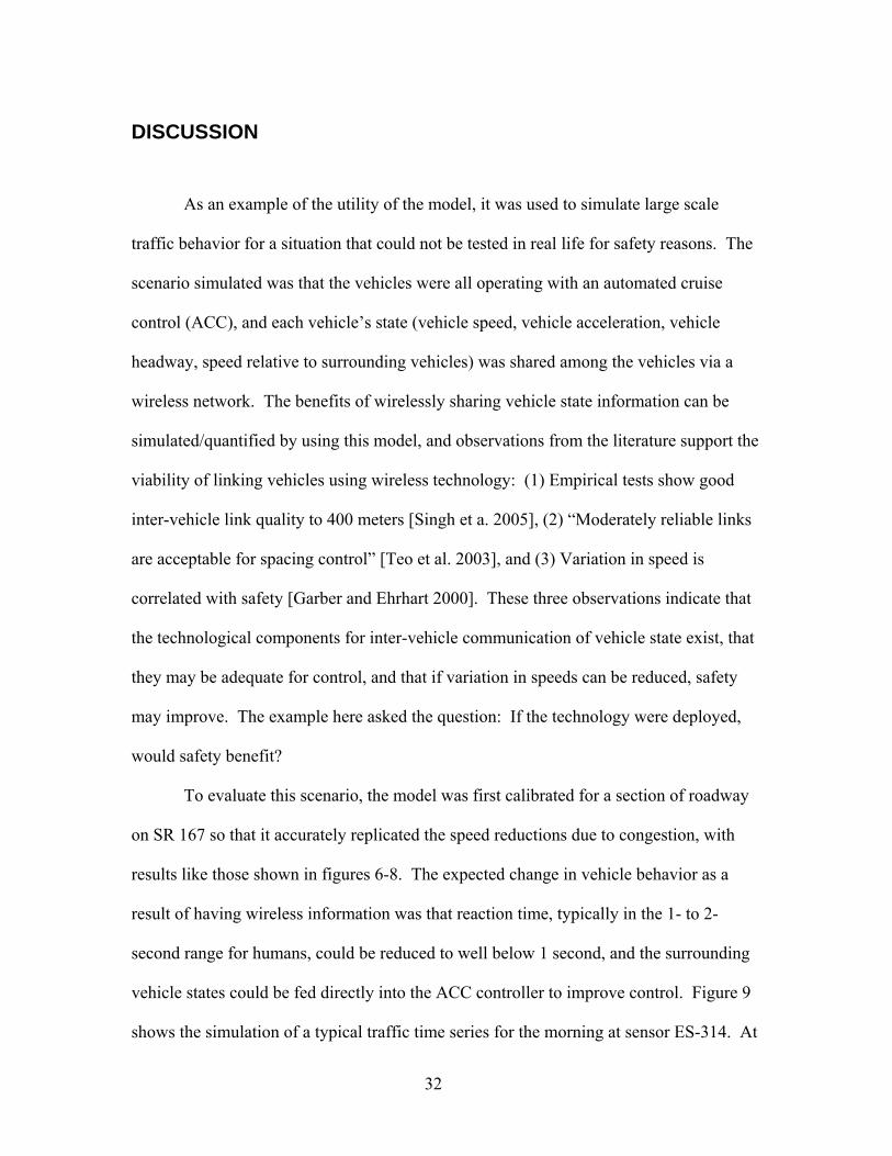
DISCUSSION

As an example of the utility of the model, it was used to simulate large scale

traffic behavior for a situation that could not be tested in real life for safety reasons. The

scenario simulated was that the vehicles were all operating with an automated cruise

control (ACC), and each vehicle’s state (vehicle speed, vehicle acceleration, vehicle

headway, speed relative to surrounding vehicles) was shared among the vehicles via a

wireless network. The benefits of wirelessly sharing vehicle state information can be

simulated/quantified by using this model, and observations from the literature support the

viability of linking vehicles using wireless technology: (1) Empirical tests show good

inter-vehicle link quality to 400 meters [Singh et a. 2005], (2) “Moderately reliable links

are acceptable for spacing control” [Teo et al. 2003], and (3) Variation in speed is

correlated with safety [Garber and Ehrhart 2000]. These three observations indicate that

the technological components for inter-vehicle communication of vehicle state exist, that

they may be adequate for control, and that if variation in speeds can be reduced, safety

may improve. The example here asked the question: If the technology were deployed,

would safety benefit?

To evaluate this scenario, the model was first calibrated for a section of roadway

on SR 167 so that it accurately replicated the speed reductions due to congestion, with

results like those shown in figures 6-8. The expected change in vehicle behavior as a

result of having wireless information was that reaction time, typically in the 1- to 2-

second range for humans, could be reduced to well below 1 second, and the surrounding

vehicle states could be fed directly into the ACC controller to improve control. Figure 9

shows the simulation of a typical traffic time series for the morning at sensor ES-314. At

32

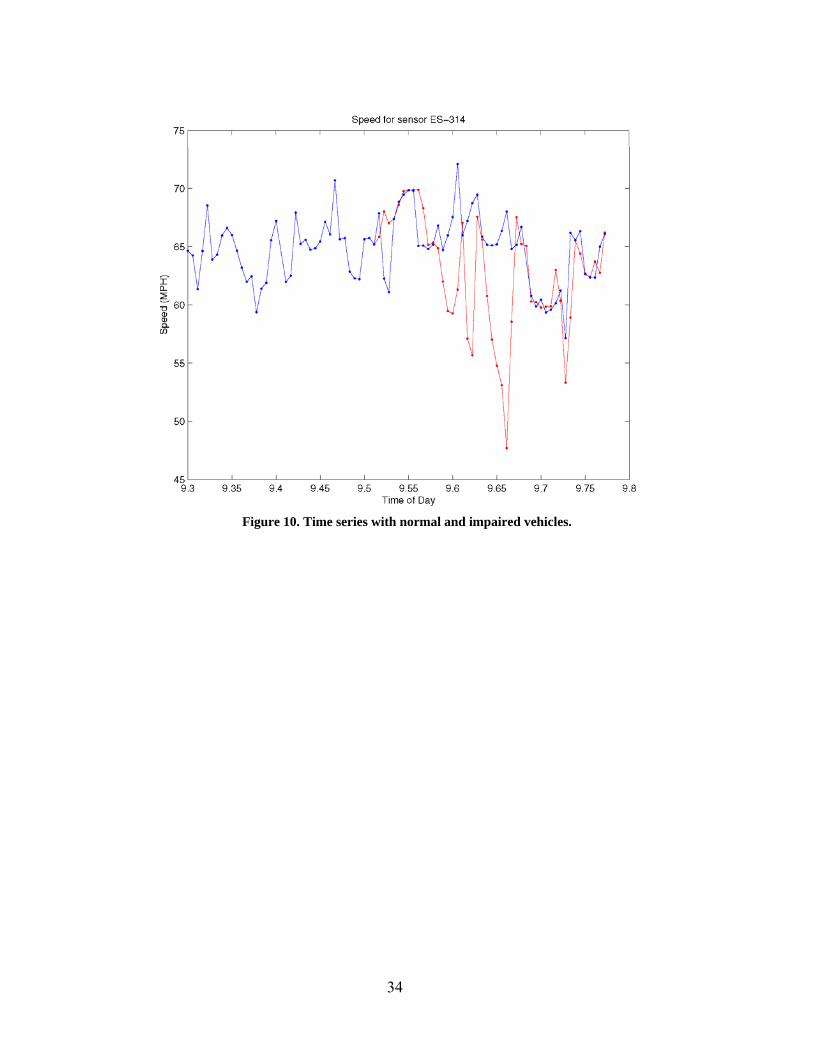
9:30 AM an impaired vehicle was injected into the flow at that location. The impairment

was modeled as a slower desired speed and a larger variability in the speed of that one

vehicle. The impaired vehicle affected overall traffic speed, as shown in red in Figure 10,

causing a sufficiently large variation in the speed, more than 10 miles per hour, that past

research has indicated may be correlated with accidents. In Figure 11 are three time

series, the original, the result of the impaired vehicle, and a black line for the traffic speed

variation that resulted when the vehicles were given inter-vehicle communication to

reduce reaction time. In this last case, variation decreased because of the collaboration

between the wirelessly connected vehicles, even though the impaired vehicle was not

collaborating.

Figure 9. Time series for typical traffic.

33

34

Figure 10. Time series with normal and impaired vehicles.

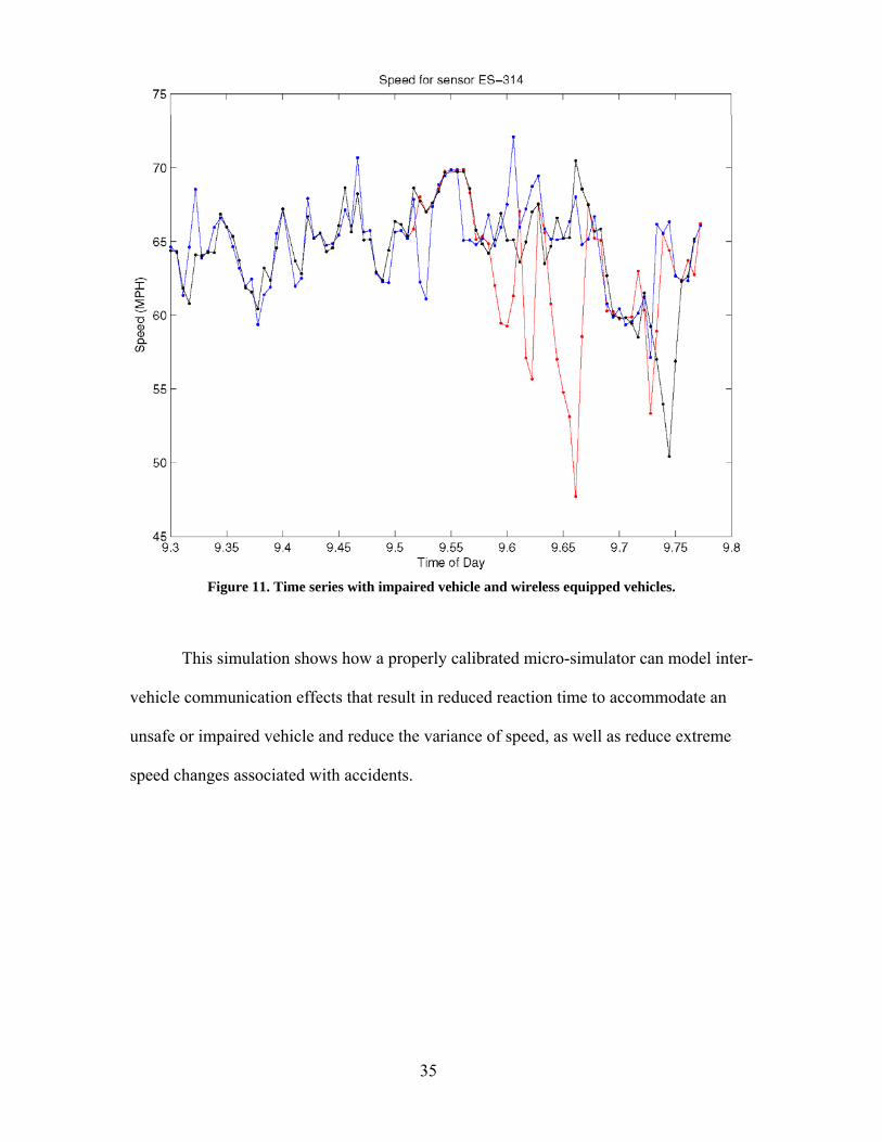
Figure 11. Time series with impaired vehicle and wireless equipped vehicles.

This simulation shows how a properly calibrated micro-simulator can model inter-

vehicle communication effects that result in reduced reaction time to accommodate an

unsafe or impaired vehicle and reduce the variance of speed, as well as reduce extreme

speed changes associated with accidents.

35

CONCLUSION

While many different microscopic traffic simulators are available today, existing

simulators are not designed to be incorporated directly into the feedback loop of a ramp

control system. This report presents a model for simulating traffic flow that can be

incorporated into a ramp metering system. The important combination of features that

this model has include (1) the ability to use real-time data as input, (2) the ability to

model an entire freeway network as a single contiguous system, and (3) the ability to

model the propagation of shockwaves that occur as a result of heavy volumes or

bottlenecks.

While the model is simple in terms of the number of parameters required to

calibrate it, it is also powerful enough to model the general behavior of traffic over long

distances, long periods of time, and varied freeway topologies. Because the parameters

are easily defined, a majority of the model parameters can be calibrated by directly

measuring parameter values from traffic sensor data. Unlike past work, this model has

been validated over a long distance by directly comparing the model output to measured

roadway data. The model is also able to take real-time sensor information as input and

then propagate the traffic model in a realistic manner. Features such as creation and

dispersion of congestion are replicated, and the shockwave phenomenon that occurs in

real traffic is duplicated. The model presented has been validated by using metrics found

in the literature. In this report, the three points of interest along the roadway that were

modeled in the simulation demonstrate that the results closely agree with real data. The

model was demonstrated to predict the evolution of traffic flow inside a region of the

36

freeway. The predictive ability of the model is a significant feature in the development of

a “simulator in the loop” control scheme.

37

IMPLEMENTATION

At this writing a student is implementing a global “simulator in the loop” ramp

control algorithm that uses the model to predict 15 minutes into the future and estimate

ramp flow rates that will mitigate the start of the shock wave phenomena. The

mathematical framework for this controller is found in section 3.3.5 of the Phase Two

report for this project. This mathematical framework is being implemented in Matlab.

This algorithmic use of the model will be compared to the existing localized control to

demonstrate improvements that can be made by using global control. Roadway data from

the TDAD data mine will be used in the validation.

38

REFERENCES

Ahmed K.I.. Modeling drivers’ acceleration and lane changing behaviors. PhD thesis. Department of Civil and Environmental Engineering. MIT. 1999.

Ayres, T.J., Li, L., Schleuning, D., and Young, D.. Preferred Time-Headway of Highway Drivers. 2001 IEEE Intelligent Transportation Systems Conference Proceedings, Oakland, USA, August 25-29, 2001. 826-829.

Bham, G., and Benekohal, R.. A High Fidelity Traffic Simulation Model Based On Cellular Automata and Car-Following Concepts. Transportation Research Part C 12C(1). 2004. 1-31.

Brackstone, M.; McDonald, M.. Driver Behavior and Traffic Modeling. Are We Looking at the Right Issues? Proceedings of 2003 Intelligent Vehicles Symposium. June 9-11, 2003. 517 – 521.

Brockfield, E., Kühne, R., and Wagner, P.. Calibration and Validation of Microscopic Traffic Flow Models. TRB 2005 Annual Meeting (CD-Rom).

Cleghorn, D., F. Hall, and D. Garbuio. Improved Data Screen Techniques for Freeway Traffic Management Systems. Transportation Research Record 1320, TRB National Research Council, Washington, D.C., 1991, pp.17-23.

Daganzo, C.F.. A Behavioral Theory of Multi-Lane Traffic Flow: Part I: Long Homogeneous Freeway Sections. Transportation Research Part B 36 (2002) 131-158.

Dailey, D., Meyers, D., Pond, L., and Guiberson, K.. Traffic Data Acquisition and Distribution (TDAD). Washington State Transportation Center - TRAC/WSDOT, Final Technical Report WA-RD 484.1, 71 pages, May 2002.

Garber, N.; Ehrhart, A. A , Effect of speed, flow, and geometric characteristics on crash frequency for two-lane highways, Transportation Research Record, , pp. 76-83 Vol. 1717, 2000

39

Jacobson, L., N. Nihan, and J. Bender. (1990). Detecting Erroneous Loop Detector Data in a Freeway Traffic Management System. Transportation Research Record 1287, TRB National Research Council, Washington, D.C., pp. 151-166.

Krishnamurthy, S., and Coifman, B.. Measuring Freeway Travel Times Using Existing Detector Infrastructure. 2004 Intelligent Transportation Systems Conference Proceedings, Washington, D.C. USA, October 3-6, 2004. 58-63.

Kyongsu, Y., Cho, Y., Lee, S., Lee, J., and Ryoo, R.. A Throttle/Brake Control Law for Vehicle Intelligent Cruise Control. Seoul 2000 FISITA World Automotive Congress June 12-15, 2000, Seoul Korea.

Singh, J.P.; Bambos, N.; Srinivasan, B.; Clawin, D.; Yonchun Yan, Empirical observations on wireless LAN performance in vehicular traffic scenarios and link connectivity based enhancements for multihop routing; 2005 IEEE Wireless Communications and Networking Conference, Volume 3, Page(s):1676 - 1682 13-17, March 2005

Subramanian, H. Estimation of car-following models. Master’s Thesis, MIT, Dept. of Civil and Environmental Engineering, Cambridge, Massachusetts, 1996.

Teo, R.; Stipanovic, D.M.; Tomlin, C.J.; Decentralized spacing control of a string of multiple vehicles over lossy datalinks, Decision and Control, 2003. Proceedings. 42nd IEEE Conference on Volume 1, 9-12Page(s):682 - 687 Dec. 2003

Theil, H.. Applied Economic Forecasting, Rand McNally, Chicago. 1966.

TRB. Highway Capacity Manual 2000. Washington, D.C.: Transportation Research Board. 2000.

Winsum, W., Heino, A.. Choice of Time-Headway in Car-Following and the Role of the Time-to-Collision information in Braking. Ergonomics 39(4). 1996. 579-92.

40

ADDITIONAL BIBLIOGRAPHY

Ametha, J., S. Turner, and S. Darbha. Formulation of a New Methodology to Identify Erroneous Paired Loop Detectors. 2001 IEEE Intelligent Transportation Systems Proceedings, 2001, pp. 591-596.

Chen, L. and A. May. Traffic Detector Errors and Diagnostics. Transportation Research Record 1132, TRB, National Research Council, Washington, D.C., 1987, pp. 82-93.

Coifman, B. Using Dual Loop Speed Traps to Identify Detector Errors. Transportation Research Record 1683, TRB National Research Council, Washington, D.C., 1999, pp. 47-58.

Coifman, B. Improved Velocity Estimation Using Single Loop Detectors. Transportation Research A, Vol. 35A, No. 10, 2001, pp. 863-880.

Dailey, D. and N. Taiyab. A Cellular Automata Model for Use with Real Freeway Data. WA-RD 537.1. Technical Report. Washington State Department of Transportation. June 2002.

Franklin, G.F., J.D. Powell, and M.L. Workman, Digital Control of Dynamic Systems, Second Edition, Addison-Wesley, 1990.

Nihan, N. Aid to Determining Freeway Metering Rates and Detecting Loop Errors. Journal of Transportation Engineering, Vol. 123, No. 6, 1997, pp. 454-458.

Zhanfeng, J., C. Chao, B. Coifman, and P. Varaiya. The PeMS Algorithms for Accurate, Real-Time Estimates of g-factors and Speeds From Single-Loop Detectors. 2001 IEEE Intelligent Transportation Systems Proceedings, 2001, pp. 536-541.

41

42