Bayesian Analysis (2010) 5, Number 2, pp. 263–282

A General Purpose Sampling Algorithm forContinuous Distributions (the t-walk)

J. Andres Christen∗ and Colin Fox†

Abstract. We develop a new general purpose MCMC sampler for arbitrary con-tinuous distributions that requires no tuning. We call this MCMC the t-walk. Thet-walk maintains two independent points in the sample space, and all moves arebased on proposals that are then accepted with a standard Metropolis-Hastingsacceptance probability on the product space. Hence the t-walk is provably con-vergent under the usual mild requirements. We restrict proposal distributions, or‘moves’, to those that produce an algorithm that is invariant to scale, and ap-proximately invariant to affine transformations of the state space. Hence scalingof proposals, and effectively also coordinate transformations, that might be usedto increase efficiency of the sampler, are not needed since the t-walk’s operationis identical on any scaled version of the target distribution. Four moves are giventhat result in an effective sampling algorithm.

We use the simple device of updating only a random subset of coordinates ateach step to allow application of the t-walk to high-dimensional problems. In a se-ries of test problems across dimensions we find that the t-walk is only a small factorless efficient than optimally tuned algorithms, but significantly outperforms gen-eral random-walk M-H samplers that are not tuned for specific problems. Further,the t-walk remains effective for target distributions for which no optimal affinetransformation exists such as those where correlation structure is very different indiffering regions of state space.

Several examples are presented showing good mixing and convergence charac-teristics, varying in dimensions from 1 to 200 and with radically different scale andcorrelation structure, using exactly the same sampler. The t-walk is available forR, Python, MatLab and C++ at http://www.cimat.mx/~jac/twalk/.

Keywords: MCMC, Bayesian inference, simulation, t-walk

1 Introduction

We develop a new MCMC sampling algorithm that contains neither adaptivity nor tun-ing parameters yet that can sample from target distributions with arbitrary scale andcorrelation structure. We dub this algorithm the “t-walk” (for “traverse” or “thought-ful” walk, as opposed to a random-walk MCMC). Unlike adaptive algorithms that at-tempt to learn the scale and correlation structure of complex target distributions (An-drieu and Thoms 2008), the t-walk is designed to be invariant to this structure. Becausethe t-walk is constructed as a Metropolis-Hastings algorithm on the product space it is

∗Centro de Investigacion en Matematicas (CIMAT), Guanajuato, Mexico, http://www.cimat.mx/

~jac†Department of Physics, University of Otago, New Zealand, mailto:fox@physics.otago.ac.nz

c© 2010 International Society for Bayesian Analysis DOI:10.1214/10-BA603

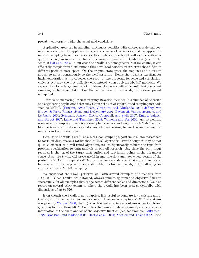
264 The t-walk

provably convergent under the usual mild conditions.

Application areas are in sampling continuous densities with unknown scale and cor-relation structure. In applications where a change of variables could be applied toimprove sampling from distributions with correlation, the t-walk will sample with ade-quate efficiency in most cases. Indeed, because the t-walk is not adaptive (e.g. in thesense of Bai et al. 2008, in our case the t-walk is a homogeneous Markov chain), it canefficiently sample from distributions that have local correlation structure that differs indifferent parts of state space. On the original state space the step size and directionappear to adjust continuously to the local structure. Hence the t-walk is excellent forinitial exploration as it overcomes the need to tune proposals for scale and correlation,which is typically the first difficulty encountered when applying MCMC methods. Weexpect that for a large number of problems the t-walk will allow sufficiently efficientsampling of the target distribution that no recourse to further algorithm developmentis required.

There is an increasing interest in using Bayesian methods in a number of scientificand engineering applications that may require the use of sophisticated sampling methodssuch as MCMC (Firmani, Avila-Reese, Ghisellini, and Ghirlanda 2007; Jeffery, vonHippel, Jefferys, Winget, Stein, and DeGennaro 2007; Bavencoff, Vanpeperstraete, andLe Cadre 2006; Symonds, Reavell, Olfert, Campbell, and Swift 2007; Emery, Valenti,and Bardot 2007; Laine and Tamminen 2008; Watzenig and Fox 2009, just to mentionsome recent examples). Therefore, developing a generic and easy to use MCMC methodlike the t-walk will help non-statisticians who are looking to use Bayesian inferentialmethods in their research fields.

Because the t-walk is useful as a black-box sampling algorithm it allows researchersto focus on data analysis rather than MCMC algorithms. Even though it may be notquite as efficient as a well-tuned algorithm, its use significantly reduces the time fromproblem specification to data analysis in one off research jobs, since the only inputrequired is the log of the target distribution and two initial points in the parameterspace. Also, the t-walk will prove useful in multiple data analyses where details of theposterior distribution depend sufficiently on a particular data set that adjustment wouldbe required to the proposal in a standard Metropolis-Hastings algorithm, allowing forautomatic use of MCMC sampling.

We show that the t-walk performs well with several examples of dimension from1 to 200. Good results are obtained, always simulating from the objective functionsuccessfully for all examples that range across different scales and dimensions. We alsoreport on several other examples where the t-walk has been used successfully, withdimensions of up to 576.

Even though the t-walk is not adaptive, it is useful to compare it to existing adap-tive algorithms, since the purpose is similar. A review of adaptive MCMC algorithmswas given by Warnes (2000, chap 1) who classified adaptive algorithms under two broadgroups as follows: those MCMC samplers that aim at updating tuning parameters usinginformation of the chain and/or of the objective function (see, for example, Gilks et al.1998; Brockwell and Kadane 2005; Haario et al. 2001; Andrieu and Thoms 2008), and

J. A. Christen and C. Fox 265

the adaptive direction samplers (ADS) that maintain several points in the state space(see, for example, Gilks et al. 1994; Gilks and Roberts 1996; Eidsvik and Tjelmeland2004) including the “evolutionary Monte Carlo” that combines ADS with moves fromgenetic algorithms to speed up a Metropolis coupled MC (Liang and Wong 2001). Thet-walk may be viewed as an adaptive sampler of the second type, since it maintains aset of two points in the state space and moves them with some structure. However,several important differences should be noted. Firstly, computational effort in the ADSscales poorly in problem dimension since the number of points maintained scales super-linearly (Gilks, Roberts, and George 1994). Consequently, even if an ADS achieves aconstant integrated autocorrelation time (IAT, see Geyer 1992) per dimension (which isoptimal, see, e.g. Roberts and Rosenthal 2001) the computation time and storage scalessuper-quadratically. In contrast the t-walk maintains two points, independent of dimen-sion, and achieves constant IAT per dimension in standard examples (see Section 4).Hence the computational effort required to achieve a given variance reduction in esti-mates scales linearly in problem dimension. Secondly, by focusing on invariance of thesampler, rather than adaptivity, we have proposed a sampler that operates efficientlyacross a wide range of target distributions, without further problem-specific work. Theinvariance property means that demonstrating the effectiveness of the t-walk for a suiteof canonical stylized test problems (as we do in Sections 3 and 4) demonstrates effec-tiveness for all problems that differ by a coordinate transformation. We are unawareof successful applications of adaptive MCMC schemes to a comprehensive suite of ob-jective functions, and note that ADS has been shown to be inefficient in many cases(see, for example, Gilks, Roberts, and George 1994). Further, the ADS requires specificmathematical calculations to be made for each objective function and in many casesthe regularity conditions for convergence are complex. In contrast, the t-walk has mildconvergence requirements since it mixes a set of standard Metropolis-Hastings kernels,and only requires evaluation of the target density.

The paper is structured as follows: in Section 2 we explain the t-walk and establishits ergodic properties (based on standard results for M-H algorithms). In Section 3.1we present several two dimensional examples and in Section 3.2 we present a morecomplex example involving a mixture of normals. In Section 4 we compare the t-walkwith optimally-tuned M-H MCMC algorithms in a suit of standard examples. Finallya discussion of the paper is given in Section 5.

2 The t-walk design

For an objective function (posterior distribution, etc.) π(x), x ∈ X (X has dimensionn and is a subset of Rn), we form the new objective function f(x, x′) = π(x)π(x′) onthe corresponding product space X × X . While a general proposal has the form

q{(y, y′) | (x, x′)},

266 The t-walk

we consider the two restricted proposals

(y, y′) =

{(x, h(x′, x)), with prob. 0.5(h(x, x′), x′), with prob. 0.5

(1)

where h(x, x′) is a random variable used to form the proposal. That is, we changeonly one of x or x′ in each step. Note, however, that we are not considering twoindependent parallel chains in each X ; instead the whole process lies in X ×X . We willrandomly choose from four different proposals, to be defined below, each characterizedby a particular function h(·, ·). We will first choose an option in (1) and second createthe proposal (y, y′) simulating from the corresponding h function.

Within a Metropolis-Hastings scheme, we need to calculate the corresponding ac-ceptance ratio. Denoting the density function of h(x, x′) by g(· | x, x′), the ratio is equalto

π(y′)π(x′)

g(x′ | y′, x)g(y′ | x′, x)

for the first case in equations 1 and

π(y)π(x)

g(x | y, x′)g(y | x, x′)

for the second case. Note that restriction to proposal 1 implies that only a singleevaluation of the target density is required, in either case.

It is straightforward to show that if the random variable h is invariant to affinetransformations, i.e. h(φx, φx′) = φh(x, x′) for any affine transformation φ, then so arethe proposals 1 and the resulting MCMC sampler. We formalize this in Theorem 1.Design of an invariant sampling algorithm then rests on the question of whether it ispossible to find one or more random variables h that give an effective sampling algorithm.We have found that the four choices for h, given below, give adequate mixing across awide range of target distributions of moderate dimension.

For high dimensional problems we select a random subset of coordinates to be up-dated at each step, as follows. In each of the four moves below we simulate a Bernoulliansequence of independent indicator variables Ij ∼ Be(p), j = 1, 2, . . . , n. If Ij = 0 coordi-nate j is not updated. The probability p of updating a given coordinate is chosen so thatnp = min(n, n1) and we set nI =

∑nj=1 Ij . That is, the expected number of parameters

to be moved at each iteration is n1 for n ≥ n1, while for n ≤ n1 all coordinates are usedin each move (we use n1 = 4, see Section 2.5).

2.1 Walk move

In many applications, particularly with weak correlations, we find that mixing of thechain is primarily achieved by a scaled random walk that we refer to as the walk move.

J. A. Christen and C. Fox 267

The walk move is defined by the function

hw(x, x′)j =

{xj +

(xj − x′j

)αj Ij = 1

xj Ij = 0,

for j = 1, 2, . . . , n, where αj ∈ R are i.i.d. r.v. with density ψw(·). Consider-ing the second case in (1), g(y|x, x′) =

∏Ij=1 gj(yj |xj , x

′j), where gj(yj |xj , x

′j) =

ψw

(yj−xj

xj−x′j

)/|xj−x′j |. It is straightforward to verify that if α = yj−xj

xj−x′j, then gj(xj |yj ,x′j)

gj(yj |xj ,x′j)=

ψw

(xj−yj

yj−x′j

)

ψw

(yj−xj

xj−x′j

)∣∣∣xj−x′j

yj−x′j

∣∣∣ =ψw( −α

1+α )ψw(α)

∣∣∣ 11+α

∣∣∣.

If α > −1 then∣∣∣ 11+α

∣∣∣ = 11+α and this proposal is symmetric ( gj(xj |yj ,x′j)

gj(yj |xj ,x′j)= 1) when

ψw

( −α

1 + α

)= (1 + α) ψw(α).

We achieve this by setting

ψw(α) =

1k√

1 + α, α ∈

[ −aw

1 + aw, aw

]

0, otherwise,

for any aw > 0, with normalizing constant k = 2(√

1 + aw − 1/√

1 + aw

). This density

is simple to simulate from using the inverse cumulative distribution as

α =aw

1 + aw

(−1 + 2u + awu2)

where u ∼ U(0, 1). Consequently, the Hastings ratio for the second case is

gw(x | y, x′)gw(y | x, x′)

= 1,

and similarly for the first case. Hence the acceptance probability is simply given by theratio of target densities (we set aw = 1.5, see Section 2.5).

2.2 Traverse move

A typical difficulty experienced by samplers using random walk moves is with densitieswith strong correlation between a few, or several, variables. A typical solution is torotate and scale coordinates of the state variables or, equivalently, the proposal distri-butions. However, that is not feasible with distributions where the correlation structurechanges through state space. (An example of such a distribution may be found inFigure 3(b).)

268 The t-walk

For those applications, efficiency of the sampler is greatly enhanced by the ‘traversemove’ defined by

ht(x, x′)j =

{x′j + β(x′j − xj) Ij = 1xj Ij = 0,

where β ∈ R+ is a r.v. with density ψt(·).The case β ≡ 0 is similar to Skilling’s leap-frog move (see MacKay 2003, sec. 30.4)

restricted to two states, and a subset of coordinates. Since the t-walk maintains justtwo states, the traverse move does not have the random selection of states required inthe leap-frog move. As noted by MacKay (2003, p. 394), this move has similaritiesto the ‘snooker’ move used in ADS. The traverse move is therefore much simpler thaneither leap-frog or snooker, and like the leapfrog move, is more widely applicable thanthe snooker move since calculation of conditional densities is not required.

Since just one random number is used in this proposal it is not possible to makeboth the proposal and the acceptance ratio independent of the dimension of state space,n, except for the case β ≡ 1. However, by setting ψt(1/β) = ψt(β), for all β > 0, theratio of proposals is simplified to βnI−2 (see below). By direct calculation it is easyto see that a density of this kind may be obtained by using a density ν(·) on R+ anddefining ψt(β) = C{ν(β−1− 1)I(0,1](β)+ ν(β− 1)I(1,∞)(β)}, for a normalizing constantC (assuming

∫ 1

0ν(β−1 − 1)dβ < ∞). A simple and convenient result is obtained with

ν(y) = (at − 1)(y + 1)−at , for any at > 1, in which case

ψt(β) =at − 12at

{(at + 1)βatI(0,1](β)}+at + 12at

{(at − 1)β−atI(1,∞](β)},

which is a mixture of two distributions and may be easily sampled from with the fol-lowing algorithm

xβ =

u

1at + 1 , with prob.

at − 12at

u

11− at , with prob.

at + 12at

,

(2)

where u ∼ U(0, 1). We want steps to be taken around the length of ||x − x′||, thus agood idea is that P (β ≤ 2) > 0.9. We set at = 6 giving P (β < 2) ≈ 0.98, see Section 2.5.A plot of ψt(β) with at = 6 is presented in Figure 1.

Following the above transformation, it is clear that

gt(y | x, x′) = ψt

( ||y − x′||||x− x′||

)||x− x′||−1.

A note of caution is prudent here, regarding calculation of the acceptance probabilityfor this move. Since the range of ht is a subspace of X it is most convenient to use thereversible jump MCMC formalism (Green and Mira 2001) for evaluating the acceptanceratio. The corresponding Jacobian determinant equals βnI−2, and since ψt(1/β) =

J. A. Christen and C. Fox 269

0.0 0.5 1.0 1.5 2.0 2.5 3.0

0.0

1.0

2.0

3.0

Beta

Den

sity

Figure 1: ψt(β) with at = 6 giving P (β < 2) ≈ 0.98.

ψt(β) the acceptance ratio isπ(y′)π(x′)

βnI−2 orπ(y)π(x)

βnI−2, for the first and second cases

in (1), respectively.

The discussion in MacKay (2003) of why Skilling’s leapfrog method works largelyapplies to the traverse move. In particular example 30.3 of MacKay (2003), and itssolution, shows that applying these moves to a Gaussian distribution in n dimensionswith covariance matrix proportional to the identity results in an expected acceptanceratio of e−2n. Hence this move has a very low acceptance ratio when applied to a largenumber of uncorrelated variables. In examples with correlation as high as 1 − 10−7,or higher, (typical of examples from inverse problems) the traverse move is effectivein mixing along the principal axis of the distribution, but is very slow in mixing indirections perpendicular to this axis. Then combining the traverse move with the othermoves in the t-walk results in an effective sampling algorithm.

2.3 Hop and Blow moves

The walk and traverse moves are not, by themselves, enough to guarantee irreducibilityof the chain over arbitrary target distributions. It is therefore necessary to introducefurther moves to ensure this. Further, both the walk and traverse moves can lead toextremely slow mixing for distributions with very high correlation (say 0.9999 or higher),as mentioned above. We find that these difficulties are somehow cured if we try to avoidx and x′ collapsing to each other. Note that the walk and traverse moves simply donot work if x = x′. We employ two further moves that make bold proposals, precisely

270 The t-walk

for avoiding x ≈ x′, but are chosen with relatively low probability (see below). We callthese moves the hop and blow moves. We have at least one bimodal example in whichswitching between modes is improved substantially by choosing the hop and blow moves10% of the time.

A hop move is defined by the function

hh(x, x′)j =

xj +σ(x, x′)

3zj Ij = 1

xj Ij = 0,

with zj ∼ N(0, 1), where σ(x, x′) = maxIj=1 |xj − x′j |. For this proposal

gh(y | x, x′) =(2π)−nI/23nI

σ(x, x′)nIexp

−

92σ(x, x′)2

∑

Ij=1

(yj − xj)2

∏

Ij=0

δxj (yj).

Note that this move is centred at x.

Finally we consider the blow move defined by

hb(x, x′)j =

{x′j + σ(x, x′)zj Ij = 1xj Ij = 0,

with zj ∼ N(0, 1). We thus have

gb(y | x, x′) =(2π)−nI/2

σ(x, x′)nIexp

−

12σ(x, x′)2

∑

Ij=1

(yj − x′j)2

∏

Ij=0

δxj (yj).

Note that, as opposed to the walk and hop moves above, this move is centred at x′.

2.4 Convergence

Let Km(·, ·) be the corresponding M-H transition kernel for proposal qm, where m ∈{w, t, h, b}. Strong aperiodicity is ensured by the positive probability of rejection in theM-H scheme. (For example, when n 6= 2, in the traverse move there is always a positive

probability that nI 6= 2 and β <(

π(x)π(y)

) 1nI−2

, resulting in an acceptance probability ofless than 1. If n = 2, and if π(·) is locally constant so that the walk and traverse movesproduce acceptance probabilities equal to 1, in such case there is a positive probabilitythat either the blow or hop moves will produce an acceptance probability less than 1.)It may be seen, using the properties of the M-H method, that each Km satisfies detailedbalance with f(x, x′). We form the transition kernel

K{(x, x′), (y, y′)} =∑

m∈{w,t,h,b}wαKm{(y, y′) | (x, x′)},

J. A. Christen and C. Fox 271

where∑

m wm = 1, which consequently also satisfies the detailed balance conditionwith f . Assuming that also K is f -irreducible (note that hop and blow moves ensuref -irreducibility), then f is the limit distribution of K (see Robert and Casella 1999,Chapter 6, for details).

2.5 Parameter settings

In our implementation of the t-walk we set the move probabilities ww, wt, wh, wb =0.4918, 0.4918, 0.0082, 0.0082 (move ratios of 60:60:1:1). These values were chosen togive the minimum integrated autocorrelation time (IAT, see Section 4), i.e. roughly thenumber of iterations per independent sample, across the two-dimensional bi-modal ex-amples presented later in Section 3. Interestingly, these values were close to optimal foreach of the example target distributions considered, and little compromise was required.

The other three important parameter settings required are n1, aw and at, the ex-pected number of parameters to be moved and the Walk and Traverse moves proposal pa-rameters, respectively. Based on many examples, those shown here and many more, weestablished reasonable test ranges for each parameter, namely n1 ∈ [2, 20], aw ∈ [0.3, 2]and at ∈ [2, 10]. We performed an optimization of these parameters by calculating theIAT’s for many examples across dimensions from n = 2 to n = 150 (we utilized theexamples presented in Section 4 running the t-walk in 500 runs of a Latin HypercubeDesign within the parameter ranges). The rounded optimal results are n1 = 4, aw = 1.5and at = 6.

Indeed, we cannot consider all possible objective functions. However, we have seenthe t-walk to succeed in sampling in many examples already (see the Discussion Sec-tion 5). Our intention is that the above parameter settings are left as default and theuser does not need to alter them to achieve a reasonable performance.

2.6 Properties

We consider that the most important property of the t-walk is that it is invariant to affinetransformations. All moves were developed with that in mind. Given a transformationof the space X , φ(z) = az + b, where a ∈ R, a 6= 0 and b ∈ Rn, that generates thenew objective function λ(z) = |a−n|π(φ−1(z)), one may generate a realization of thet-walk either by applying the t-walk kernel with λ as objective function, with startingvalues (x0, x

′0) ∈ φ(X )×φ(X ), or by applying the t-walk kernel to π with starting values

(φ−1(x0), φ−1(x′0)), and then transforming the resulting chain with φ. The followingTheorem states that the t-walk is invariant to changes in scale and reference point.

Theorem 1. Let V ∈ X ×X and A ⊂ X ×X (a measurable set). The t-walk transitionkernel using objective λ(z) = |a−n|π(φ−1(z)), Kλ, and the t-walk kernel using objectiveπ, Kπ, have the invariance property

Kλ(φ(V ), φ(A)) = Kπ(V, A). (3)

Proof: Let W ′ = (y, y′) ∈ φ(X )×φ(X ). Elementary calculations show that |a−nI |qm(

272 The t-walk

φ−1(W ) | V ) = qm(W | φ(V )) for m = w, b, h and |a−1|qt(φ−1(W ) | V ) = qt(W | φ(V ))(in this case the transformation is univariate, that is, along the line xj−x′j , and thereforethe necessary Jacobian is simply |a−1|; in what follows we will take in this case n′I = 1and n′I = nI for the other moves). It is clear that the M-H acceptance probabilityconsidering proposal m for λ is (let f ′(W ′) = λ(y)λ(y′))

ρλm(φ(V ),W ′) = min

{1,

f ′(W ′)f ′(φ(V ))

qm(φ(V )|W ′)qm(W ′|φ(V ))

}.

Equivalently for π

ρπm(V, φ−1(W ′)) = min

{1,

f(φ−1(W ′))f(V )

qm(V |φ−1(W ′))qm(φ−1(W ′)|V )

}.

Since f(φ−1(W ′)) = |a2n|f ′(W ′) and f(V ) = |a2n|f ′(φ(V )), and the above relationon the qm’s, we see that ρλ

m(φ(V ), W ′) = ρπm(V, φ−1(W ′)). It is clear then that the

probabilities of accepting a jump have the property

rλm(φ(V ), φ(A)) =

∫φ(A)

ρλm(φ(V ),W ′)qm(W ′ | φ(V ))dW ′ =∫

φ(A)ρπm(V, φ−1(W ′))|a−n′I |qm(φ−1(W ′) | V )dW ′ =∫

Aρπm(V, W )|a−n′I |qm(W | V )|an′I |dW = rπ

m(V,A).

Since the t-walk kernel is a mixture of the individual kernels for m = w, t,b,h, andtogether with the fact that the probability of not jumping in either case is the same(1− rλ

m(φ(V ), φ(X × X )) = 1− rπm(V,X × X )), establishes the result. ¥

It is immediate that the above result also holds for n steps into the t-walk andtherefore Kn

π (V,A) = Knλ (φ(V ), φ(A)) and since also f(A) = f ′(φ(A)) we have that

||Knπ (V, ·)− f(·)||TV = ||Kn

λ (φ(V ), ·)− f ′(·)||TV .

The above establishes the following characteristic of the t-walk; its performance(speed of convergence, autocorrelations, etc) remain unchanged with a change in scaleand position as given by φ. More importantly, for many applications, the t-walk iseffectively invariant for more general classes of transformations. When all componentsare selected, i.e. nI = n, Theorem 1 remains valid for the t-walk limited to the traverseand walk moves with the more general change in scale using a = diag(aj), a diagonalmatrix, with aj ∈ R \ {0}. While the hop and blow moves are not invariant under thistransformation, the operation of those moves is effectively unchanged. Further, whena represents a rotation, the traverse move is invariant while the remaining moves areeffectively invariant. In particular, the density over the walk move is invariant. Whena is allowed to be any nonsingular matrix, i.e. φ is a general invertible affine transfor-mation, the traverse move remains invariant. The simple form of coordinate selectionthat we employ for high dimensional problems means that these further invariances donot actually hold in general, however the operation of the sampler does not suffer andit appears that the beneficial consequences of the invariances are preserved.

J. A. Christen and C. Fox 273

Although the t-walk contains random walk type updates, it may not be reducedsolely to a random walk MCMC in the usual sense. Since xn and x′n both have π(·)as limit distribution, then ||x(t) − x′(t)|| is a property of π and in the limit has thedistribution of the distance between two points sampled independently from π. Hencethe “step size” (in some loose sense) cannot actually be manipulated or designed in anyway. However, when viewed as a sampler on the original space, the step size appears toadapt to the characteristics of shape and size of the section of π that is being analyzed.

3 Numerical Examples

3.1 2-dimensional examples

We present some simple examples with two parameters. First we experiment with abimodal, correlated, objective function that has the form

π(x) = C exp

{−τ

(2∑

i=1

(xi −m1,i)2)(

2∑

i=1

(xi −m2,i)2)}

, (4)

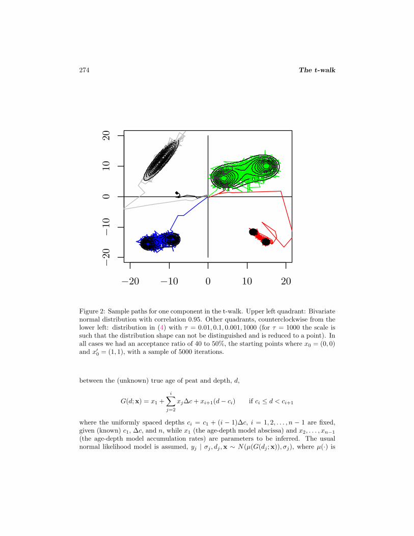
for some (m1,1,m1,2) and (m2,1,m2,2) that approximately locate two modes (on R2), andscale parameter τ (C is a normalization constant). In Figure 2 we present an illustrationof the t-walk sample paths over quite different choices of the above distribution, andalso on a correlated bivariate normal istribution.

We present two further quite extreme two dimensional examples. Figure 3(a) showsa mixture of two rather contrasting bivariate normals, one flat, oval highly correlatedmode and one peaked low correlated, forming an objective function with two modes.Figure 3(b) shows a strongly correlated hook shape objective function with thin edgesand a thicker mid section where the mode is (see Figure 3 for more details).

Note that we have run the t-walk over seven quite different objective functions,varying radically in scale, correlation, modes, etc. The t-walk performed well and moreor less similarly in all cases. Next we present a more complex example of dimension 15.

3.2 Higher dimension example

In this section we demonstrate the usefulness of the t-walk in a high dimension example,that arises as the posterior distribution over a semiparametric age model for radiocarboncalibration in paleoecology. In that work, cores taken from peat bogs are sectioned andthen subject to radiocarbon dating, from which we wish to build a model for age as afunction of depth. See Blaauw and Christen (2005) for details.

For a single core we have a series of radiocarbon determinations with standard errorsyj±σj taken at depth dj for j = 1, 2, . . . ,m. Hence {yj , σj , dj}j=1,2,...,m are the (known)measured data. We follow Blaauw and Christen (2005), who take the measured valuesof σj and dj to be the true values, and use a piecewise linear model for the relation

274 The t-walk

−20 −10 0 10 20

−20

−10

010

20

0.1

0.2

0.3 0.1

0.2

0.3

0.1

0.2

0.3

0.4

0.5

0.1

0.2

0.3

0.4

0.5

0.00

5

0.01

0.015

0.00

5

0.01

0.015

Figure 2: Sample paths for one component in the t-walk. Upper left quadrant: Bivariatenormal distribution with correlation 0.95. Other quadrants, counterclockwise from thelower left: distribution in (4) with τ = 0.01, 0.1, 0.001, 1000 (for τ = 1000 the scale issuch that the distribution shape can not be distinguished and is reduced to a point). Inall cases we had an acceptance ratio of 40 to 50%, the starting points where x0 = (0, 0)and x′0 = (1, 1), with a sample of 5000 iterations.

between the (unknown) true age of peat and depth, d,

G(d;x) = x1 +i∑

j=2

xj∆c + xi+1(d− ci) if ci ≤ d < ci+1

where the uniformly spaced depths ci = c1 + (i − 1)∆c, i = 1, 2, . . . , n − 1 are fixed,given (known) c1, ∆c, and n, while x1 (the age-depth model abscissa) and x2, . . . , xn−1

(the age-depth model accumulation rates) are parameters to be inferred. The usualnormal likelihood model is assumed, yj | σj , dj ,x ∼ N(µ(G(dj ;x)), σj), where µ(·) is

J. A. Christen and C. Fox 275

−5 0 5 10 15

−15

−5

05

10

15

1e−04 1e−04

1e−04

0.0022 0.0022

0.0043

0.0064

0.00

85

0.0106

1e−04 1e−04

1e−04

0.0022 0.0022

0.0043

0.0064

0.00

85

0.0106

−3 −2 −1 0 1 2 3 4

05

10

15

(a) (b)

Figure 3: Sample points for one component in the t-walk (a) mixture of bivariatenormals, low mode with weight 0.7, µ1 = 6, σ1 = 4, µ2 = 0, σ2 = 5, ρ = 0.8, high modewith weight 0.3, µ1 = −3, σ1 = 1, µ2 = 10, σ2 = 1, ρ = 0.1. We took 100,000 iterationswith an acceptance rate of around 45%. (b) “Rosenbrock” (Rosenbrock 1960) densityequal to π(x, y) = C exp

[−k{100(y − x2)2 + (1− x)2

}](for some normalizing constant

C), with k = 1/20. We used 100,000 iterations. This is quite a difficult density to plotand we needed to chop off the two tips of the hook so the corresponding algorithm in Rcould plot the contours correctly. In this case we obtained an acceptance ratio of about13% with 100,000 points, lower than all other examples presented in this Section 3.1.

the radiocarbon calibration curve, see Blaauw and Christen (2005) for details.

Additionally, a (prior) model is proposed for the (peat accumulation) rates xj =wxj+1 +(1−w)zj , where w ∼ Beta(αw, βw) and zj ∼ Gamma(αz, βz). Here αw, βw, αz

and βz are known (representing the prior information available on accumulation rates,see Blaauw and Christen 2005). Therefore, the unknown parameters to be sampledby the t-walk are x1, . . . , xn−1, and w that we denote xn thus the unknown set ofparemeters may be written as the n-vector x.

A simple program (in C++) is used to calculate − log f(x|{yj , σj , dj}j=1,2,...,m).Restricted support of parameters (eg. w ∈ [0, 1]) is enabled in most implementationsof the t-walk by providing a ‘Supp’ function that returns True or False according towhether or not the input x is in the support of the objective function (in the MatLabimplementation the function providing the log target density returns the value -Inf forarguments outside its support). The other inputs required are the starting values for xand x′.

In this example we set xn = w = 0.4, x′n = w′ = 0.1, draw xn−1, x′n−1 ∼

Gamma(αz, βz), and take xj = wxj+1 + (1 − w)zj and x′j = w′x′j+1 + (1 − w′)z′j for

276 The t-walk

60 80 100 120 140

2000

3000

4000

Depth, cm

Cale

ndar

Yea

rs B

P

w

Den

sity

0.00 0.05 0.10 0.15

05

10

15

20

(a) (b)

Figure 4: (a) MAP estimator (red) and two sample age-depth models for core EngXV.For each of the m = 57 radiocarbon determinations a sample of 25 calendar ages weresimulated and plotted (small dots; calendar ages measured in ‘years Before Present’(BP), where ‘present’ is AD 1950). (b) Histogram for the marginal posterior distributionof w.

j = n− 2, . . . , 2 drawing zj , z′j ∼ Gamma(αz, βz). Finally, we draw x1, x

′1 ∼ N(y1, σ1).

This provides initial, random, values for x and x′ that are in the support of the objectivefunction.

We used the data set called “EngXV” with m = 57 determinations (Blaauw, vanGeel, Mauquoy, and van der Plicht 2004), using n = 71 (70 parameters for the age-depthmodel plus w) and ran 300,000 iterations of the t-walk (taking 1 minute on a MacBookPro lap top). Two sample age-depth models and the MAP estimator are presented inFigure 4(a), and a histogram approximating the marginal distribution of w is presentedin Figure 4(b).

4 Comparisons with optimally-tuned M-H MCMC

Roberts and Rosenthal (2001) present a review of optimal scaling for a random-walkMetropolis Hastings (M-H) algorithm applied to some simple models. For minimumintegrated autocorrelation time (IAT), the proposal window must be tuned to give anacceptance rate of 0.234, for the type of models considered by them. In particular,they consider the objective π(x) =

∏dj=1 Cjg(Cjxj), where g is the standard Normal

distribution, with the values Cj = 1 (model 1), C1 = 2 and Cj = 1; j = 2, 3, . . . , n(model 2), and C1 = 1 and Cj ∼ Exp(1); j = 2, 3, . . . , n (model 3). Also we consider

J. A. Christen and C. Fox 277

Cj = 10 (model 0). We have already mentioned that a finely tuned MCMC for a par-ticular objective function should be more or equally efficient than any generic method,including the t-walk. However, fine tuning a M-H MCMC constitutes significant effortin applying the method. While very flexible and very general indeed, a M-H MCMCcan be extremely ineffective and, in high dimensions, very difficult to tune. Avoidingthis difficulty is the idea behind adaptive methods (see Andrieu and Thoms, 2008, fora recent review), and the t-walk.

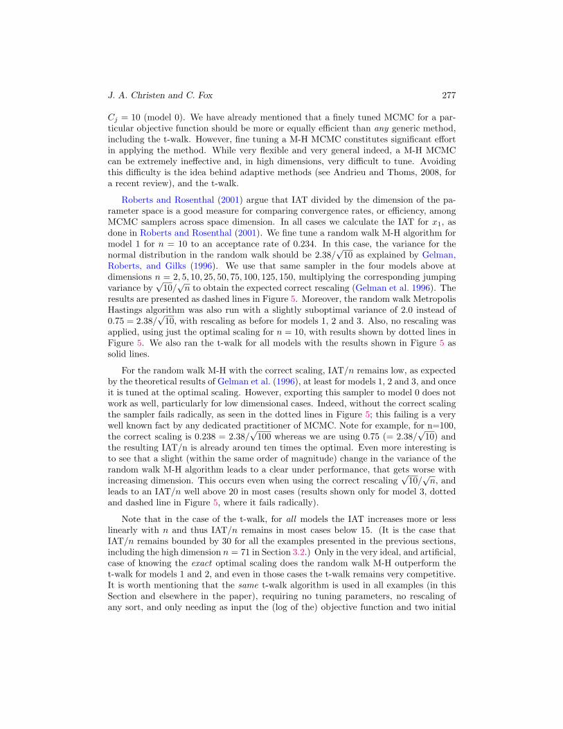
Roberts and Rosenthal (2001) argue that IAT divided by the dimension of the pa-rameter space is a good measure for comparing convergence rates, or efficiency, amongMCMC samplers across space dimension. In all cases we calculate the IAT for x1, asdone in Roberts and Rosenthal (2001). We fine tune a random walk M-H algorithm formodel 1 for n = 10 to an acceptance rate of 0.234. In this case, the variance for thenormal distribution in the random walk should be 2.38/

√10 as explained by Gelman,

Roberts, and Gilks (1996). We use that same sampler in the four models above atdimensions n = 2, 5, 10, 25, 50, 75, 100, 125, 150, multiplying the corresponding jumpingvariance by

√10/

√n to obtain the expected correct rescaling (Gelman et al. 1996). The

results are presented as dashed lines in Figure 5. Moreover, the random walk MetropolisHastings algorithm was also run with a slightly suboptimal variance of 2.0 instead of0.75 = 2.38/

√10, with rescaling as before for models 1, 2 and 3. Also, no rescaling was

applied, using just the optimal scaling for n = 10, with results shown by dotted lines inFigure 5. We also ran the t-walk for all models with the results shown in Figure 5 assolid lines.

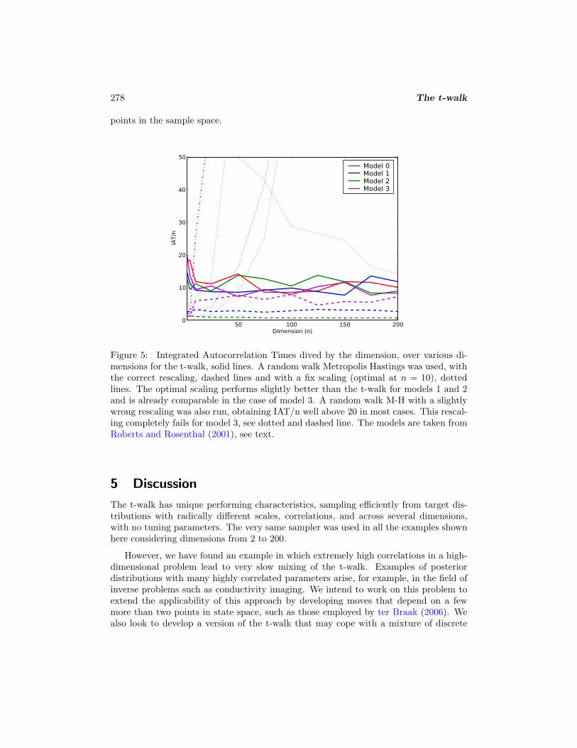
For the random walk M-H with the correct scaling, IAT/n remains low, as expectedby the theoretical results of Gelman et al. (1996), at least for models 1, 2 and 3, and onceit is tuned at the optimal scaling. However, exporting this sampler to model 0 does notwork as well, particularly for low dimensional cases. Indeed, without the correct scalingthe sampler fails radically, as seen in the dotted lines in Figure 5; this failing is a verywell known fact by any dedicated practitioner of MCMC. Note for example, for n=100,the correct scaling is 0.238 = 2.38/

√100 whereas we are using 0.75 (= 2.38/

√10) and

the resulting IAT/n is already around ten times the optimal. Even more interesting isto see that a slight (within the same order of magnitude) change in the variance of therandom walk M-H algorithm leads to a clear under performance, that gets worse withincreasing dimension. This occurs even when using the correct rescaling

√10/

√n, and

leads to an IAT/n well above 20 in most cases (results shown only for model 3, dottedand dashed line in Figure 5, where it fails radically).

Note that in the case of the t-walk, for all models the IAT increases more or lesslinearly with n and thus IAT/n remains in most cases below 15. (It is the case thatIAT/n remains bounded by 30 for all the examples presented in the previous sections,including the high dimension n = 71 in Section 3.2.) Only in the very ideal, and artificial,case of knowing the exact optimal scaling does the random walk M-H outperform thet-walk for models 1 and 2, and even in those cases the t-walk remains very competitive.It is worth mentioning that the same t-walk algorithm is used in all examples (in thisSection and elsewhere in the paper), requiring no tuning parameters, no rescaling ofany sort, and only needing as input the (log of the) objective function and two initial

278 The t-walk

points in the sample space.

50 100 150 200Dimension (n)

0

10

20

30

40

50

IAT/n

Model 0Model 1Model 2Model 3

Figure 5: Integrated Autocorrelation Times dived by the dimension, over various di-mensions for the t-walk, solid lines. A random walk Metropolis Hastings was used, withthe correct rescaling, dashed lines and with a fix scaling (optimal at n = 10), dottedlines. The optimal scaling performs slightly better than the t-walk for models 1 and 2and is already comparable in the case of model 3. A random walk M-H with a slightlywrong rescaling was also run, obtaining IAT/n well above 20 in most cases. This rescal-ing completely fails for model 3, see dotted and dashed line. The models are taken fromRoberts and Rosenthal (2001), see text.

5 Discussion

The t-walk has unique performing characteristics, sampling efficiently from target dis-tributions with radically different scales, correlations, and across several dimensions,with no tuning parameters. The very same sampler was used in all the examples shownhere considering dimensions from 2 to 200.

However, we have found an example in which extremely high correlations in a high-dimensional problem lead to very slow mixing of the t-walk. Examples of posteriordistributions with many highly correlated parameters arise, for example, in the field ofinverse problems such as conductivity imaging. We intend to work on this problem toextend the applicability of this approach by developing moves that depend on a fewmore than two points in state space, such as those employed by ter Braak (2006). Wealso look to develop a version of the t-walk that may cope with a mixture of discrete

J. A. Christen and C. Fox 279

and continuous parameters.

We believe that the t-walk is already a useful improvement on existing attemptsat creating automatic, generic, self adjusting, MCMC’s. The current design results ina simple, mathematically tractable algorithm that lends itself to use as a black-boxsampler, since only evaluation of the objective function is needed; there being no needto calculate any conditional distributions, etc. nor some prior knowledge of the numberof modes, tails etc. As presented in the numerical examples, we have evidence thatthe t-walk will perform satisfactorily with common densities (posterior distributions incommon Bayesian statistical analyses). For these problems the t-walk can be used as ablack-box simulation technique, either for exploratory analysis of the objective densityat hand or for final MCMC simulation.

Besides the examples we have already mentioned, we and other colleagues haveimplemented the t-walk in a series problems. Indeed, we now treat the t-walk as oursampler of first choice and have been pleasantly surprised to find that it always providesuseful output, and avoids several of the difficulties seen in standard MCMC. Theseexamples include a reliability example (n = 2), reservoir effects in radiocarbon datingproblems (n = 3− 6), a bacterial horizontal gene transfer model (n > 50, Zenil-Lopez2008), electrical capacitance tomography using polygonal representations (n = 32−128,where not having to calculate Jacobians for subspace moves was very liberating), pixel-based impedance imaging (n = 576), and in fitting analytic models to groundwaterpump tests (n = 2− 15). We have also combined the t-walk kernel with Gibbs kernels,when the full conditionals for some blocks of parameters have known distributions andthe rest have full conditionals that are difficult to sample from. Such examples arosein fitting spatial Gaussian (n = 2) processes and other in an Econometric time seriesmodel (n = 9, Lence, Hart, and Hayes 2009).

The t-walk is available as an R (R Development Core Team 2008) and Pythonhttp://www.python.org/ packages (and is also available in MatLab and C++) athttp://www.cimat.mx/~jac/twalk/ and will soon be included in the PyMC packageat http://code.google.com/p/pymc/.

ReferencesAndrieu, C. and Thoms, J. (2008). “A tutorial on adaptive MCMC.” Statistics and

Computing , 18(4): 343–373. 263, 264

Bai, Y., Roberts, G., and Rosenthal, J. (2008). “On the Containment Condition forAdaptive Markov Chain Monte Carlo Algorithms.” Technical report, No. 0806, De-partment of Statistics, University of Toronto. 264

Bavencoff, F., Vanpeperstraete, J., and Le Cadre, J. (2006). “Constrained bearings-onlytarget motion analysis via Markov chain Monte Carlo methods.” IEEE Transactionson Aerospace and Electrical Systems, 42(4): 1240–1263. 264

Blaauw, M. and Christen, J. (2005). “Radiocarbon peat chronologies and environmentalchange.” Applied Statistics, 54(4): 805–816. 273, 275

280 The t-walk

Blaauw, M., van Geel, B., Mauquoy, D., and van der Plicht, J. (2004). “Radiocar-bon wiggle-match dating of peat deposits: advantages and limitations.” Journal ofQuaternary Science, 19: 177–181. 276

Brockwell, A. and Kadane, J. (2005). “Identification of Regeneration Times in MCMCSimulation, With Application to Adaptive Schemes.” Journal of Computational andGraphical Statistics, 14(2): 436–458. 264

Eidsvik, J. and Tjelmeland, H. (2004). “On directional Metropolis-Hastings algorithms.”Statistics and Computing , 16(1): 93–106. 265

Emery, A. F., Valenti, E., and Bardot, D. (2007). “Using Bayesian inference for param-eter estimation when the system response and experimental conditions are measuredwith error and some variables are considered as nuisance variables.” MeasurementScience & Technology , 18(1): 19–29. 264

Firmani, C., Avila-Reese, V., Ghisellini, G., and Ghirlanda, G. (2007). “Long gamma-ray burst prompt emission properties as a cosmological tool.” Revista Mexicana deAstronomia y Astrofısica, 43: 203–216. 264

Gelman, A., Roberts, G., and Gilks, W. (1996). “Efficient Metropolis jumping rules.”In Bernardo J.M, D. A., Berger J.O. and A.M.F., S. (eds.), Bayesian Statistics V ,599–608. Oxford: Oxford University Press. 277

Geyer, C. (1992). “Practical Markov Chain Monte Carlo.” Statistical Science, 7(4):473–511. 265

Gilks, W. and Roberts, G. (1996). “Strategies for improving MCMC.” In Gilks, W.,Richardson, S., and Spiegelhalter, D. (eds.), Markov Chain Monte Carlo in Practice,89–114. London: Chapman and Hall. 265

Gilks, W., Roberts, G., and George, E. (1994). “Adaptive direction sampling.” TheStatistician, 43: 179–189. 265

Gilks, W., Roberts, G., and Sahu, S. (1998). “Adaptive Markov Chain Monte CarloThrough Regeneration.” Journal of the American Statistical Association, 93: 1045–1054. 264

Green, P. and Mira, A. (2001). “Delayed Rejection in Reversible Jump Metropolis–Hastings.” Biometrika, 88: 1035–1053. 268

Haario, H., Saksman, E., and Tamminen, J. (2001). “An adaptive Metropolis algo-rithm.” Bernoulli, 7: 223–242. 264

Jeffery, E. J., von Hippel, T., Jefferys, W. H., Winget, D. E., Stein, N., and DeGennaro,S. (2007). “New techniques to determine ages of open clusters using white dwarfs.”Astrophysical Journal, 658(1): 391–395. 264

Laine, M. and Tamminen, J. (2008). “Aerosol model selection and uncertainty modellingby adaptive MCMC technique.” Atmospheric Chemistry and Physics, 8(24): 7697–7707. 264

J. A. Christen and C. Fox 281

Lence, S. C., Hart, C., and Hayes, D. (2009). “An Econometric Analysis of the Structureof Commodity Futures Prices (poster paper).” In Agricultural & Applied EconomicsAssociation & American Council on Consumer Interests 2009 Joint Annual Meeting,26-28 July . Milwaukee, Wisconsin, US. 279

Liang, F. and Wong, W. (2001). “Real-parameter evolutionary Monte Carlo with appli-cations to Bayesian mixture models.” Journal of the American Statistical Association,96(454): 653–666. 265

MacKay, D. J. C. (2003). Information Theory, Inference, and Learning Algorithms.Cambrige, UK: Cambridge University Press. 268

R Development Core Team (2008). R: A Language and Environment for StatisticalComputing . R Foundation for Statistical Computing, Vienna, Austria. ISBN 3-900051-07-0.URL http://www.R-project.org/ 279

Robert, C. and Casella, G. (1999). Monte Carlo Statistical Methods. Springer Texts inStatistics. New York: Springer. 271

Roberts, G. O. and Rosenthal, J. S. (2001). “Optimal scaling for various Metropolis-Hastings algorithms.” Statistical Science, 16(4): 351–367. 265, 276, 277, 278

Rosenbrock, H. (1960). “An automatic method for finding the greatest or least value ofa function.” The Computer Journal, 3: 175–184. 275

Symonds, J. P. R., Reavell, K., Olfert, J., Campbell, B., and Swift, S. (2007). “Dieselsoot mass calculation in real-time with a differential mobility spectrometer.” Journalof Aerosol Science, 38(1): 52–68. 264

ter Braak, C. (2006). “A Markov Chain Monte Carlo version of the genetic algorithmDifferential Evolution: easy Bayesian computing for real parameter spaces.” Statisticsand Computing , 16: 239–249. 278

Warnes, G. (2000). “The Normal Kernel Coupler: An adaptive Markov Chain MonteCarlo method for efficiently sampling from multi-modal distributions.” Ph.D. thesis,University of Washington. 264

Watzenig, D. and Fox, C. (2009). “A review of statistical modelling and inference forelectrical capacitance tomography.” Measurement Science and Technology , 20(5):(052002) 1–22. 264

Zenil-Lopez, R. (2008). “A Hidden Markov Model of Horizontal Gene Transfer in Bacte-ria.” Master’s thesis, Centro de Investigacion en Matematicas, Guanajuato, Mexico.279

Acknowledgments

J Andres Christen was partially founded by grant SEMARNAT-2004-C01-0007 (Mexico). Wethank Sergio Lence, Rosana Zenil, Patricia Bautista, Jose Miguel Ponciano and Sergio PerezE. for enthusiastic feedback on implementing and using the t-walk.

282 The t-walk