A GENERAL LIMIT THEOREM FOR ... - math.uni-frankfurt.deneiningr/asynorm.pdf · LIMIT LAWS FOR...

The Annals of Applied Probability2004, Vol. 14, No. 1, 378–418© Institute of Mathematical Statistics, 2004

A GENERAL LIMIT THEOREM FOR RECURSIVE ALGORITHMSAND COMBINATORIAL STRUCTURES

BY RALPH NEININGER1 AND LUDGER RÜSCHENDORF

McGill University and Universität Freiburg

Limit laws are proven by the contraction method for random vectors ofa recursive nature as they arise as parameters of combinatorial structuressuch as random trees or recursive algorithms, where we use the Zolotarevmetric. In comparison to previous applications of this method, a generaltransfer theorem is derived which allows us to establish a limit law on thebasis of the recursive structure and the asymptotics of the first and secondmoments of the sequence. In particular, a general asymptotic normality resultis obtained by this theorem which typically cannot be handled by the morecommon �2 metrics. As applications we derive quite automatically manyasymptotic limit results ranging from the size of tries or m-ary search treesand path lengths in digital structures to mergesort and parameters of randomrecursive trees, which were previously shown by different methods one byone. We also obtain a related local density approximation result as well as aglobal approximation result. For the proofs of these results we establish that asmoothed density distance as well as a smoothed total variation distance canbe estimated from above by the Zolotarev metric, which is the main tool inthis article.

1. Introduction. This work gives a systematic approach to limit laws forsequences of random vectors that satisfy distributional recursions as they appearunder various models of randomness for parameters of trees, characteristicsof divide-and-conquer algorithms or, more generally, for quantities related torecursive structures. While there are also strong analytic techniques for thesubject, we extend and systematize a more probabilistic approach—the contractionmethod. This method was first introduced for the analysis of Quicksort in [48] andfurther developed independently in [49] and [47]; see also the survey article byRösler and Rüschendorf [51]. The name of the method refers to the fact that theanalysis makes use of an underlying map of measures, which is a contraction withrespect to some probability metric.

Our article is a continuation of the article by Neininger [41], who used the�2 metric approach to establish a general limit theorem for multivariate divide-and-conquer recursions, thus extending the one-dimensional results in [50]. Althoughthe �2 approach works well for many problems that lead to nonnormal limit

Received October 2001; revised January 2003.1Supported by NSERC Grant A3450 and the Deutsche Forschungsgemeinschaft.AMS 2000 subject classifications. Primary 60F05, 68Q25; secondary 68P10.Key words and phrases. Contraction method, multivariate limit law, asymptotic normality, ran-

dom trees, recursive algorithms, divide-and-conquer algorithm, random recursive structures,Zolotarev metric.

378

LIMIT LAWS FOR RECURSIVE ALGORITHMS 379

distributions, its main defect is that it does not work for an important class ofproblems that lead to normal limit laws. We discuss this problem in more detailin Section 2 and, to overcome this problem, we propose to use, as alternativemetrics, the Zolotarev metrics ζs , which are more flexible and at the same timestill manageable. The advantage of alternative metrics such as the Zolotarevmetrics for the analysis of algorithms has been demonstrated for some examplesin [47] and [10].

The flexibility of the ζs metrics is in the fact that while for s = 2, we reobtainthe common �2 theory, we also can use ζs with s > 2, which gives access tonormal limit laws, or with s < 2, which leads to results where we can weakenthe assumption of finite second moments—an assumption that is usually presentin the �2 approach.

In his 1999 article, Pittel [44] stated as a heuristic principle that various globalcharacteristics of large size combinatorial structures such as graphs and treesare asymptotically normal if the mean and variance are “nearly linear” in n.As a technical reason, he argued that the normal distribution with the sametwo moments “almost” satisfies the recursion. He exemplified this idea by theindependence number of uniformly random trees. An essential step in the proof ofour limit theorem is the introduction of an accompanying sequence which fulfillsapproximatively a recursion of the same form as the characteristics do and isformulated essentially in terms of the limiting distribution. This is similar to thetechnical idea proposed by Pittel [44].

We obtain a general limit theorem for divide-and-conquer recursions where theconditions are formulated in terms of relationships of moments and a conditionthat ensures the asymptotic stability of the recursive structure. These conditionscan quite easily be checked in a series of examples and allow us to (re)derive manyexamples from the literature. In fact, for the special case of normal limit laws, weneed—according to Pittel’s principle—the first and second moment to apply themethod; see Corollary 5.2.

Several further metrics can be estimated from above by the Zolotarev metric.We prove that, in any dimension, a smoothed density distance and the smoothedtotal variation distance are estimated from above by a Zolotarev metric. Asa consequence we obtain a local density approximation result and a globalapproximation property for general recursive algorithms.

We investigate sequences of d-dimensional vectors (Yn)n∈N0 , which satisfy thedistributional recursion

YnD=

K∑r=1

Ar(n)Y(r)

I(n)r

+ bn, n ≥ n0,(1)

where (A1(n), . . . ,AK(n), bn, I(n)

), (Y(1)n ), . . . , (Y

(K)n ) are independent, A1(n),

. . . ,AK(n) are random d × d matrices, bn is a random d-dimensional vector,I (n) is a vector of random cardinalities I

(n)r ∈ {0, . . . , n} and (Y

(1)n ), . . . , (Y

(K)n )

380 R. NEININGER AND L. RÜSCHENDORF

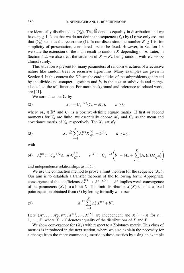
are identically distributed as (Yn). The D= denotes equality in distribution and wehave n0 ≥ 1. Note that we do not define the sequence (Yn) by (1); we only assumethat (Yn) satisfies the recurrence (1). In our discussion, the number K ≥ 1 is, forsimplicity of presentation, considered first to be fixed. However, in Section 4.3we state the extension of the main result to random K depending on n. Later, inSection 5.2, we also treat the situation of K = Kn being random with Kn → ∞almost surely.

This situation is present for many parameters of random structures of a recursivenature like random trees or recursive algorithms. Many examples are given inSection 5. In this context the I

(n)r are the cardinalities of the subproblems generated

by the divide-and-conquer algorithm and bn is the cost to subdivide and merge,also called the toll function. For more background and reference to related work,see [41].

We normalize the Yn by

Xn := C−1/2n (Yn − Mn), n ≥ 0,(2)

where Mn ∈ Rd and Cn is a positive-definite square matrix. If first or second

moments for Yn are finite, we essentially choose Mn and Cn as the mean andcovariance matrix of Yn, respectively. The Xn satisfy

XnD=

K∑r=1

A(n)r X

(r)

I(n)r

+ b(n), n ≥ n0,(3)

with

A(n)r := C−1/2

n Ar(n)C1/2

I(n)r

, b(n) := C−1/2n

(bn − Mn +

K∑r=1

(Ar(n)M

I(n)r

))(4)

and independence relationships as in (1).We use the contraction method to prove a limit theorem for the sequence (Xn).

Our aim is to establish a transfer theorem of the following form: Appropriateconvergence of the coefficients A

(n)r → A∗

r , b(n) → b∗ implies weak convergence

of the parameters (Xn) to a limit X. The limit distribution L(X) satisfies a fixedpoint equation obtained from (3) by letting formally n → ∞:

XD=

K∑r=1

A∗rX

(r) + b∗.(5)

Here (A∗1, . . . ,A

∗K,b∗),X(1), . . . ,X(K) are independent and X(r) ∼ X for r =

1, . . . ,K , where X ∼ Y denotes equality of the distributions of X and Y .We show convergence for (Xn) with respect to a Zolotarev metric. This class of

metrics is introduced in the next section, where we also explain the necessity fora change from the more common �2 metric to these metrics by using an example


of a fixed-point equation of the form (5) related to the normal distribution. Thenwe study contraction properties of fixed-point equations (5) with respect to thesemetrics in Section 3 and give a transfer theorem as desired in Section 4. The restof the article is devoted to applications of our general transfer result, where we(re)derive various central limit laws for random recursive structures, ranging fromthe size of m-ary search trees or random tries path lengths in digital search trees,tries and Patricia tries, via top-down mergesort, and the maxima in right trianglesto parameters of random recursive trees and plane-oriented versions thereof.

2. The Zolotarev metric. The contraction method applied in this article isbased on certain regularity properties of the probability metrics used for provingconvergence of the parameters as well as on some lower and upper bounds for thesemetrics. A probability metric τ = τ (X,Y ) defined for random vectors X and Y ingeneral depends on the joint distribution of (X,Y ). The probability metric τ iscalled simple if τ (X,Y ) = τ (µ, ν) depends only on the marginal distributionsµ and ν of X and Y . Most of the metrics used in this article are simple and thereforeinduce a metric on (a subclass of ) all probability measures on R

d . A simple metricτ is called ideal of order s > 0 if

τ (X + Z,Y + Z) ≤ τ (X,Y )(6)

for all Z independent of X and Y , and

τ (cX, cY ) = |c|sτ (X,Y )

for all c �= 0. Note that τ (X,Y ) = τ (µ, ν) depends only on the marginaldistributions µ and ν of X and Y .

The �2 metric defined by

�2(µ, ν) = inf{‖X − Y‖2 :X ∼ µ, Y ∼ ν

}has been used frequently in the analysis of algorithms since its introduction inthis context by Rösler [48] for the analysis of Quicksort (see, e.g., [39, 41, 42]);note that �2 is ideal of order 1. This implies that �2 typically cannot be used forfixed-point equations that occur for the normal distribution such as

Xd= 1√

2X1 + 1√

2X2

d=: T X,(7)

where Xr are independent copies of X. Here we consider T as a map T :M → Mon the space M of univariate probability measures with T µ := L(Z1/

√2 +

Z2/√

2), where Z1 and Z2 are independent with distribution µ, and we abbreviateT X := T L(X). For centered X and Y with finite second moment, we may chooseindependent optimal couplings (X1, Y1), (X2, Y2) of (X,Y ), that is, vectors that


satisfy �2(X,Y ) = ‖Xr − Yr‖2, r = 1,2. Then we have

�22(T X,T Y ) ≤

∥∥∥∥ 1√2(X1 − Y1)

∥∥∥∥2

2+∥∥∥∥ 1√

2(X2 − Y2)

∥∥∥∥2

2

=((

1√2

)2

+(

1√2

)2)�2

2(X,Y )

= �22(X,Y ).

This suggests that restriction of T to the space M12(0) of univariate centered

probability measures with finite second moment is not a strict contraction in �2,which would be essential for application of the contraction method. In fact, T isnot a contraction on M1

2(0) in any metric. This results from the fact that all thecentered normal distributions are (exactly) the fixed points of T . On the otherhand, strict contraction would imply uniqueness of the fixed point.

The basic idea is to refine the working space. We restrict T to the subspaceM1

s (0, σ 2) ⊂ M12(0), 2 < s ≤ 3, where the variance of the measures is fixed to

be σ 2 > 0 and a finite absolute sth moment is assumed. In our example (7) thefixed point is then unique and, in fact, we can prove the contraction property in theZolotarev metrics ζs .

Zolotarev [57] found the following metric ζs , which is ideal of order s > 0,defined for d-dimensional vectors by

ζs(X,Y ) = supf ∈Fs

∣∣E(f (X) − f (Y )

)∣∣,(8)

where for s = m + α, 0 < α ≤ 1, m ∈ N0,

Fs := {f ∈ Cm(Rd,R) :

∥∥f (m)(x) − f (m)(y)∥∥ ≤ ‖x − y‖α

}.

Convergence in ζs implies weak convergence and moreover, for some c > 0,

cζs(X,Y ) ≥{

E(‖X‖s − ‖Y‖s),

π1+s(‖X‖,‖Y‖),where π is the Prohorov metric (see [58]). There are upper bounds for ζs in termsof difference pseudomoments

κs(X,Y ) = sup{|Ef (X) − f (Y )| :‖f (x) − f (y)‖ ≤ ∥∥‖x‖s−1x − ‖y‖s−1y

∥∥}.Note that κs is the minimal metric of the compound metric

τs(X,Y ) = E∥∥‖X‖s−1X − ‖Y‖s−1Y

∥∥,(9)

that is, κs(µ, ν) = inf{τs(X,Y ) :X ∼ µ,Y ∼ ν}, and, therefore, allows estimatesin terms of moments. We also use that κs and �s are topologically equivalenton spaces of random variables with uniformly bounded absolute sth moment.Finiteness of ζs(X,Y ) implies that X and Y have identical mixed moments up to


order m. Mixed moments are the expectations of products of powers of coordinatesof a multivariate random variable. The order of a mixed moment is the sum of theexponents in such a product. For X and Y such that all mixed moments up toorder m are zero and moments of order s are finite, we have that

ζs(X,Y ) ≤ (1 + α)

(1 + s)s(X,Y ),(10)

where

s(X,Y ) = 2mκs(X,Y ) + (2κs(X,Y ))α[min(Ms

X,MsY )]1−α

.(11)

Here MsX and Ms

Y are the absolute moments of X and Y of order s. From (11) weobtain, in particular, for α = 1 (i.e., s ∈ N),

ζs(X,Y ) ≤ (2m + s)κs(X,Y ).

For s ∈ N, finiteness of ζs(X,Y ) does not need finiteness of sth absolute momentsand so ζs also can be applied to stable distributions, for example.

For proving convergence to a normal distribution, ζs is well suited for s > 2. Thereason for this is that the operator T in (7) that characterizes the normal distributionis a contraction on M1

s (0, σ 2) with respect to ζs ,

ζs(T X,T Y ) = ζs

(1√2X1 + 1√

2X2,

1√2Y1 + 1√

2Y2

)

≤ ζs

(1√2X1,

1√2Y1

)+ ζs

(1√2X2,

1√2Y2

)

≤((

1√2

)s

+(

1√2

)s)ζs(X,Y ),

and we have 2(1/√

2 )s < 1. Note, however, that by normalization typically onlythe first two moments can be matched and so the range of application is restrictedto s ≤ 3. For linear transformations A, one obtains

ζs(AX,AY ) ≤ ‖A‖sopζs(X,Y ),(12)

where ‖A‖op := sup‖x‖=1 ‖Ax‖ is the operator norm of A (see [58]). Some furtherproperties are established throughout the article.

3. Contraction and fixed-point properties. In this section random affinetransformations of multivariate measures are studied. Given a vector (A1, . . . ,

AK,b) of random d × d matrices A1, . . . ,AK and a random d-dimensionalvector b, we associate the transformation

T :Md → Md, µ �→ L

(K∑

r=1

ArZ(r) + b

).(13)


Here (A1, . . . ,AK,b),Z(1), . . . ,Z(K) are assumed to be independent, Z(r) ∼ µ forr = 1, . . . ,K and Md denotes the space of d-dimensional probability measures. If(A1, . . . ,AK,b) has components with finite absolute sth moments and ‖µ‖s :=(E|Z|s)(1/s)∨1 < ∞, then, by independence, ‖T µ‖s < ∞. In the followingdiscussion, Lipschitz and contraction properties of T with respect to the Zolotarevmetric ζs are crucial. To have ζs(µ, ν) < ∞ we assume that µ and ν have finiteabsolute sth moments and that all mixed moments of µ,ν of orders less than s areequal. In this case the following Lipschitz property, which is an extension of (12),holds:

LEMMA 3.1. Let (A1, . . . ,AK,b) and T be given as in (13), and letµ,ν ∈ Md with ‖µ‖s ,‖ν‖s < ∞ and identical mixed moments of orders lessthan s. Let (A1, . . . ,AK,b) be s-integrable. Then we have

ζs(T µ,T ν) ≤(

E

K∑r=1

‖Ar‖sop

)ζs(µ, ν).(14)

PROOF. By independence we have ‖T µ‖s,‖T ν‖s < ∞. For given (A1, . . . ,

AK,b) the mixed moments of order less than s of T µ depend only on the mixedmoments of µ of order less than s. Thus T µ and T ν have identical mixed momentsof order less than s. This implies ζs(T µ,T ν) < ∞. The s-homogeneity of ζs

with respect to linear transformations given in (12) implies, with the notationϒ = L(A1, . . . ,AK,b) and α = (α1, . . . , αK),

ζs(T µ,T ν)

= ζs

(K∑

r=1

ArZ(r) + b,

K∑r=1

ArW(r) + b

)

= supf ∈Fs

{∣∣∣∣∣E[f

(K∑

r=1

ArZ(r) + b

)− f

(K∑

r=1

ArW(r) + b

)]∣∣∣∣∣}

= supf ∈Fs

{∣∣∣∣∣∫

E

[f

(K∑

r=1

αrZ(r) + β

)− f

(K∑

r=1

αrW(r) + β

)]dϒ(α,β)

∣∣∣∣∣}

(15)

≤∫

supf ∈Fs

{∣∣∣∣∣E[f

(K∑

r=1

αrZ(r) + β

)− f

(K∑

r=1

αrW(r) + β

)]∣∣∣∣∣}

dϒ(α,β)

=∫

ζs

(K∑

r=1

αrZ(r) + β,

K∑r=1

αrW(r) + β

)dϒ(α,β)

≤∫ K∑

r=1

‖αr‖sopζs(µ, ν) dϒ(α,β) =

(E

K∑r=1

‖Ar‖sop

)ζs(µ, ν),


where Z(1), . . . ,Z(K),W(1), . . . ,W(K), (A1, . . . ,AK,b) are independent withZ(r) ∼ µ and W(r) ∼ ν. �

REMARK. With respect to the �2 metric, the corresponding contractionproperty is (see [5, 41])

�2(T µ,T ν) ≤∥∥∥∥∥E

K∑r=1

AtrAr

∥∥∥∥∥op

�2(µ, ν).

Since ‖E∑K

r=1(AtrAr)‖op ≤ E

∑Kr=1 ‖At

rAr‖op = E∑K

r=1 ‖Ar‖2op, the contraction

condition for �2 is weaker than that for the comparable ζ2 and, therefore, it ispreferable to apply �2 compared to ζ2 if it applies. Note, however, that in the one-dimensional case both conditions are identical and only first moments have to becontrolled for the application of ζ2 and �2. In comparison to the �p metrics, theζs metrics allow the exponent s in (14) to vary and thus are a much more flexibletool compared to the �p metrics.

From the point of view of applications, we can scale only the first and secondmixed moments. Therefore, in particular, the cases 0 < s ≤ 3 are of interest. For2 < s ≤ 3 we have to control the mean and the covariances to obtain the finitenessof the ζs metric. We define for 2 < s ≤ 3, a vector m ∈ R

d , and for a symmetricpositive semidefinite d × d matrix C, the space

Mds (m,C) := {

µ ∈ Md :‖µ‖s < ∞,Eµ = m, Cov(µ) = C}.(16)

Then ζs is finite on Mds (m,C) × Md

s (m,C) for all 2 < s ≤ 3, m ∈ Rd and

symmetric positive semidefinite C. For the sake of short notation, we also writeMd

s (m,C) for 0 < s ≤ 2; this same term for 1 < s ≤ 2 denotes the subspaceof probability distributions with finite sth moment and mean m (the C has nomeaning). For 0 < s ≤ 1, the m and C have no meaning, and Md

s (m,C) thendenotes the space of probability distributions on R

d with finite sth moment; thus,

Mds (m,C) := {µ ∈ Md : ‖µ‖s < ∞,Eµ = m}, 1 < s ≤ 2,(17)

:= {µ ∈ Md :‖µ‖s < ∞}, 0 < s ≤ 1.(18)

A direct calculation yields the ranges of the restriction of T to the set Mds (m,C):

LEMMA 3.2. Let (A1, . . . ,AK,b) and T be given as in (13) with (A1, . . . ,

AK,b) being s-integrable for some 0 < s ≤ 3. Then it holds that

T(Md

s (m,C))⊂ Md

s (mT ,CT )


with

mT :=(

E

K∑r=1

Ar

)m + Eb(19)

and

CT := E[bbt] + E

K∑r=1

(ArCAtr)

(20)

+ E

[(K∑

r=1

Ar

)mbt

]+ E

[(K∑

r=1

Ar

)mbt

]t

.

We are interested in fixed points of the map T in certain subsets of Md . To thisaim we consider, for a fixed (A1, . . . ,Ak, b), some m ∈ R

d and some symmetricpositive semidefinite d × d matrix C such that

m = mT , C = CT .

Then, by Lemma 3.2, T maps Mds (m,C) into Md

s (m,C) for all 0 < s ≤ 3.Moreover, by Lemma 3.1, T is a contraction on (Md

s (m,C), ζs) if

E

K∑r=1

‖Ar‖sop < 1.

Next we prove the existence and uniqueness of a fixed point of T in Mds (m,C).

LEMMA 3.3. Let (A1, . . . ,AK,b) and T be given as in (13) with (A1, . . . ,

AK,b) being s-integrable for some 0 < s ≤ 3. Let m ∈ Rd and let a symmetric

positive semidefinite d × d matrix C be given such that m = mT and C = CT

[defined in (19) and (20)]. If the contraction condition

ξ := E

K∑r=1

‖Ar‖sop < 1

is satisfied, then the restriction of T to Mds (m,C) has a unique fixed point.

PROOF. We choose µ0 ∈ Mds (m,C) and define µn := T (µn−1) = T (n)(µ0)

for n ≥ 1. Then for all p ∈ N we have, by Lemma 3.1,

ζs(µn,µn+p) ≤p−1∑i=0

ζs(µn+i,µn+i+1)

≤ ζs(µ0,µ1)

p−1∑i=0

ξn+i

≤ ζs(µ0,µ1)ξn

1 − ξ→ 0


as n → ∞. Thus (µn) is a Cauchy sequence in the metric space (Mds (m,C), ζs).

By the lower estimate of ζs in the Lévy metric, we obtain that (µn) convergesweakly to a µ ∈ Md . The weak convergence, the independence properties in thedefinition of T and the continuity of the affine transformation imply T µn → T µ

weakly; thus we have that µ = T µ is a fixed point of T . For random variablesXn and X with L(Xn) = µn and L(X) = µ, and with the estimate |E‖Xn‖s −E‖Xm‖s | ≤ constζs(µn,µm) [see (9)], we have that the real sequence (‖µn‖s) isa Cauchy sequence and, therefore, bounded. This implies the uniform integrabilityof {|Xn|s :n ∈ N} for all 0 < s < s, which together with the convergence indistribution implies Xn → X in Ls . Since EXn = m for all n ∈ N in the cases > 1 and additionally Cov(Xn) = C for all n ∈ N in the case s > 2, this impliesEX = m and Cov(X) = C in these cases, respectively. By the lemma of Fatou,E‖X‖s < ∞; thus L(X) ∈ Md

s (m,C). For the uniqueness, let µ,ν ∈ Mds (m,C)

be fixed points of T . Then

ζs(T µ,T ν) ≤(

E

K∑r=1

‖Ar‖sop

)ζs(µ, ν);

thus ζs(µ, ν) = 0 and µ = ν. �

REMARK. Svante Janson pointed out to us that the metric spaces (Mds (m,

C), ζs) are complete, which, by Banach’s fixed-point theorem, implies theassertion of Lemma 3.3 as well.

Subsequently, Idd denotes the d × d identity matrix. The previous considera-tions yield:

COROLLARY 3.4. Let (A1, . . . ,AK,b) and T be given as in (13) with(A1, . . . ,AK,b) being s-integrable, 0 < s ≤ 3 and E

∑Kr=1 ‖Ar‖s

op < 1. Assume

Eb =

0 and E[bbt ] + E∑K

r=1(ArAtr) = Idd , if 2 < s ≤ 3,

0, if 1 < s ≤ 2.

Then T has a unique fixed point in Mds (0, Idd).

4. The main convergence theorem.

4.1. Convergence in the Zolotarev metrics. We return to the situation outlinedin the Introduction. Given is a sequence (Yn) of random vectors satisfying therecurrence

YnD=

K∑r=1

Ar(n)Y(r)

I(n)r

+ bn, n ≥ n0,(21)


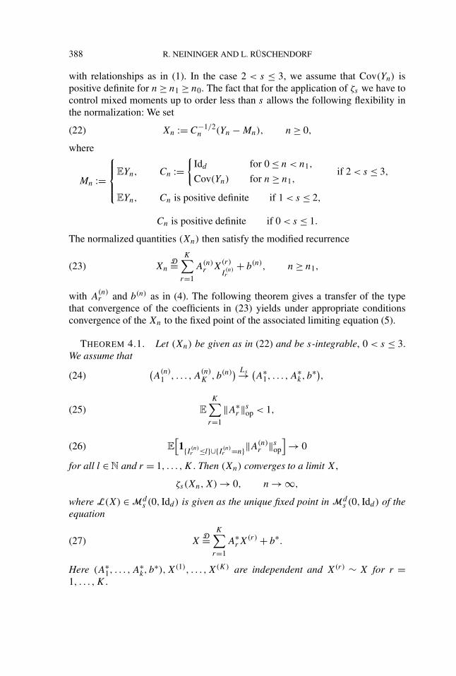
with relationships as in (1). In the case 2 < s ≤ 3, we assume that Cov(Yn) ispositive definite for n ≥ n1 ≥ n0. The fact that for the application of ζs we have tocontrol mixed moments up to order less than s allows the following flexibility inthe normalization: We set

Xn := C−1/2n (Yn − Mn), n ≥ 0,(22)

where

Mn :=

EYn, Cn :={

Idd for 0 ≤ n < n1,

Cov(Yn) for n ≥ n1,if 2 < s ≤ 3,

EYn, Cn is positive definite if 1 < s ≤ 2,

Cn is positive definite if 0 < s ≤ 1.

The normalized quantities (Xn) then satisfy the modified recurrence

XnD=

K∑r=1

A(n)r X

(r)

I(n)r

+ b(n), n ≥ n1,(23)

with A(n)r and b(n) as in (4). The following theorem gives a transfer of the type

that convergence of the coefficients in (23) yields under appropriate conditionsconvergence of the Xn to the fixed point of the associated limiting equation (5).

THEOREM 4.1. Let (Xn) be given as in (22) and be s-integrable, 0 < s ≤ 3.We assume that (

A(n)1 , . . . ,A

(n)K , b(n)) Ls→ (

A∗1, . . . ,A

∗k, b

∗),(24)

E

K∑r=1

‖A∗r ‖s

op < 1,(25)

E

[1{I (n)

r ≤l}∪{I (n)r =n}‖A(n)

r ‖sop

]→ 0(26)

for all l ∈ N and r = 1, . . . ,K . Then (Xn) converges to a limit X,

ζs(Xn,X) → 0, n → ∞,

where L(X) ∈ Mds (0, Idd) is given as the unique fixed point in Md

s (0, Idd) of theequation

XD=

K∑r=1

A∗rX

(r) + b∗.(27)

Here (A∗1, . . . ,A

∗k, b

∗),X(1), . . . ,X(K) are independent and X(r) ∼ X for r =1, . . . ,K .


PROOF. For 2 < s ≤ 3, the sequence (Xn) in (23) is standardized; thus weobtain the relationships

Eb(n) = 0, Eb(n)(b(n))t + E

K∑r=1

(A(n)

r (A(n)r )t

)= Idd , n ≥ n1.(28)

For 1 < s ≤ 2, the sequence (Xn) is centered; thus Eb(n) = 0. Thus from theconvergence in Ls in (24) we obtain

Eb∗ = 0, E[b∗(b∗)t ] + E

K∑r=1

(A∗

r (A∗r )

t)= Idd

in the case 2 < s ≤ 3 and Eb∗ = 0 for 1 < s ≤ 2. Therefore, by Corollary 3.4,there exists a unique fixed point L(X) ∈ Md

s (0, Idd) of (27) in Mds (0, Idd) for all

0 < s ≤ 3.We introduce the accompanying sequence

Qn :D=K∑

r=1

A(n)r

(1{I (n)

r <n1}X(r)

I(n)r

+ 1{I (n)r ≥n1}X

(r))

+ b(n), n ≥ n1,

where (A(n)1 , . . . ,A

(n)K , b(n), I (n)),X(1), . . . ,X(K), (X

(1)n ), . . . , (X

(K)n ) are indepen-

dent with X(r) ∼ X and X(r)j ∼ Xj for r = 1, . . . ,K, j = 0, . . . , n1 − 1. Since

L(X) ∈ Mds (0, Idd) and comparing the definition of Qn for 2 < s ≤ 3 with Xn

in (23), we deduce Cov(Qn) = Cov(Xn); hence L(Qn) ∈ Mds (0, Idd) for all

n ≥ n1 and thus ζs distances between Xn, Qn and X are finite for n ≥ n1. Weobtain from the triangle inequality

ζs(Xn,X) ≤ ζs(Xn,Qn) + ζs(Qn,X).(29)

First we show that ζs(Qn,X) → 0. This is a consequence of the upper boundin (10) and of the convergence of the pseudomoments κs(Qn,X) → 0 whichfollows from �s(Qn,X) → 0, since absolute moments of order s are bounded

for (Qn): With the representation XD=∑K

r=1 A∗rX

(r) + b∗, we obtain

�s(Qn,X) ≤∥∥∥∥∥

K∑r=1

(A∗

r − 1{I (n)r ≥n1}A

(n)r

)X(r)

∥∥∥∥∥s

+ ∥∥b(n) − b∗∥∥s

+∥∥∥∥∥

K∑r=1

1{I (n)r <n1}A

(n)r X

(r)

I(n)r

∥∥∥∥∥s

≤K∑

r=1

(∥∥A∗r − A(n)

r

∥∥s +

∥∥∥1{I (n)r <n1}‖A

(n)r ‖op

∥∥∥s

)‖X‖s + ∥∥b(n) − b∗∥∥

s(30)

+K∑

r=1

∥∥∥∥∥n1−1∑j=0

1{I (n)r =j }A

(n)r X

(r)j

∥∥∥∥∥s

.(31)


The three summands in (30) converge to zero by (24) and (26). The summandin (31) tends to zero using (26) by∥∥∥1{I (n)

r =j }A(n)r X

(r)j

∥∥∥s

≤∥∥∥1{I (n)

r =j }‖A(n)r ‖op‖X(r)

j ‖∥∥∥s

≤∥∥∥1{I (n)

r <n1}‖A(n)r ‖op

∥∥∥s

sup0≤j<n1

‖Xj‖s .

The first summand in (29) is estimated similarly to (15). Let ϒn denote the jointdistribution of (A

(n)1 , . . . ,A

(n)K , b(n), I (n)) and α = (α1, . . . , αK), j = (j1, . . . , jK).

Then with

pn := E

K∑r=1

(1{I (n)

r =n}‖A(n)r ‖s

op

)→ 0, n → ∞,

we obtain, for n ≥ n1,

ζs(Xn,Qn)

= ζs

(K∑

r=1

A(n)r X

(r)

I(n)r

+ b(n),

K∑r=1

A(n)r

(1{I (n)

r <n1}X(r)

I(n)r

+ 1{I (n)r ≥n1}X

(r))

+ b(n)

)

(32)

≤∫

ζs

(K∑

r=1

αrX(r)jr

,

K∑r=1

αr

(1{jr<n1}X

(r)jr

+ 1{jr≥n1}X(r)))

dϒn(α,β, j)

≤∫ K∑

r=1

1{jr≥n1}‖αr‖sopζs(Xjr ,X)dϒn(α,β, j)

≤ pnζs(Xn,X) +(

E

K∑r=1

‖A(n)r ‖s

op

)sup

n1≤j≤n−1ζs(Xj ,X).

Thus with (29) it follows that

ζs(Xn,X) ≤ 1

1 − pn

[(E

K∑r=1

‖A(n)r ‖s

op

)sup

n1≤j≤n−1ζs(Xj ,X) + o(1)

].

This implies that (ζs(Xn,X)) is bounded. Let η := supn≥n1ζs(Xn,X) and η :=

lim supn→∞ ζs(Xn,X), and let ε > 0 be arbitrary. There exists an l ∈ N with


ζs(Xn,X) ≤ η + ε for all n ≥ l. We deduce, using (33), (29) and (24),

ζs(Xn,X) ≤ 1

1 − pn

[∫ K∑r=1

1{n1≤jr≤l}‖αr‖sopζs(Xjr ,X)dϒn(α,β, j)

+∫ K∑

r=1

1{l<jr<n}‖αr‖sopζs(Xjr ,X)dϒn(α,β, j)

]

≤ η

1 − pn

E

K∑r=1

(1{n1≤I

(n)r ≤l}‖A(n)

r ‖sop

)+ η + ε

1 − pn

E

K∑r=1

‖A(n)r ‖s

op

≤(

E

K∑r=1

‖Ar‖sop

)(η + ε) + o(1).

With n → ∞ we obtain

η ≤(

E

K∑r=1

‖Ar‖sop

)(η + ε).

Since ε > 0 is arbitrary and E∑K

r=1 ‖Ar‖sop < 1, we obtain η = 0. Hence

ζs(Xn,X) → 0. �

4.2. Other metrics. Theorem 4.1 yields convergence of Xn to X w.r.t. theζs metric, where X is the unique fixed point of (27) in Md

s (0, Idd) under thecontraction condition E

∑Kr=1 ‖A∗

r‖sop < 1. It is of interest that several related

convergence results are obtainable for further metrics by similar arguments or byupper bounds for these metrics in terms of the Zolotarev metric ζs . We show thatthis, in particular, leads to local and global approximation results.

For random vectors X and Y with densities fX and fY , let

�(X,Y ) = ess supx∈Rd

|fX(x) − fY (x)|

denote the sup distance of the densities. Let θ be a random vector with a smoothdensity fθ . We say that fθ satisfies the Hölder condition (Hr), r = m + α,0 < α ≤ 1, if

(Hr)∥∥f (m)

θ (x) − f(m)θ (y)

∥∥≤ Cr(θ)‖x − y‖α.(33)

By means of θ we introduce a smoothed version �r of the distance �. Define�r = �r,θ by

�r (X,Y ) = suph∈R

|h|r�(X + hθ,Y + hθ).

Smoothing metrics have been used for proving central limit theorems fornormalized sums and for martingales in probability theory (cf. [45, 46, 53]).


PROPOSITION 4.2 (Regularity of �r ). Let r > d and θ satisfy condition(Hr−d). Then �r is a probability metric ideal of order r − d and

�r (X,Y ) ≤ Cr−d(θ)ζr−d(X,Y ),(34)

where Cr(θ) is the Hölder constant in (33).

PROOF. The probability metric property and property (6) are easy to establish.To see that �r is ideal of order r − d , let c �= 0. Then

�r (cX, cY ) = suph∈R

|h|r ess supx∈Rd

∣∣fcX+hθ (x) − fcY+hθ (x)∣∣

= suph∈R

|h|r ess supx∈Rd

∣∣fc(X+(h/c)θ)(x) − fc(Y+(h/c)θ)(x)∣∣

= 1

|c|d suph∈R

|h|r ess supx∈Rd

∣∣∣∣fX+(h/c)θ

(x

c

)− fY+(h/c)θ

(x

c

)∣∣∣∣= 1

|c|d suph∈R

|h|r ess supx∈Rd

∣∣fX+(h/c)θ (x) − fY+(h/c)θ(x)∣∣

= |c|r−d �r(X,Y ).

To prove (34) note that

�r (X,Y ) = suph∈R

|h|r ess supx∈Rd

∣∣fh(X/h+θ)(x) − fh(Y/h+θ)(x)∣∣

= suph∈R

|h|r−d ess supx∈Rd

∣∣∣∣fX/h+θ

(x

h

)− fY/h+θ

(x

h

)∣∣∣∣= sup

h∈R

|h|r−d�

(X

h+ θ,

Y

h+ θ

).

If θ satisfies condition (Hr−d), then we obtain with H = PX − PY , wherePX denotes the distribution of X,

�(X + θ,Y + θ) = ess supx∈Rd

∣∣∣∣∫

fθ (x − y) dH(y)

∣∣∣∣≤ Cr−d(θ)ζr−d(X,Y ),

since for any x, fθ(x − ·) is a Hölder function of order r − d with Hölder constantCr−d(θ). Therefore,

|h|r�(X + hθ,Y + hθ) = |h|r−d�

(X

h+ θ,

Y

h+ θ

)

≤ |h|r−dCr−d(θ)ζr−d

(X

h,Y

h

)

= Cr−d(θ)ζr−d(X,Y ).


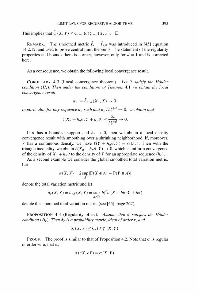
This implies that �r (X,Y ) ≤ Cr−d(θ)ζr−d(X,Y ). �

REMARK. The smoothed metric �r = �r,θ was introduced in [45] equation14.2.12, and used to prove central limit theorems. The statement of the regularityproperties and bounds there is correct, however, only for d = 1 and is correctedhere.

As a consequence, we obtain the following local convergence result.

COROLLARY 4.3 (Local convergence theorem). Let θ satisfy the Höldercondition (Hs). Then under the conditions of Theorem 4.1 we obtain the localconvergence result

αn := �s+d(Xn,X) → 0.

In particular, for any sequence hn such that αn/hs+dn → 0, we obtain that

�(Xn + hnθ,Y + hnθ) ≤ αn

hs+dn

→ 0.

If θ has a bounded support and hn → 0, then we obtain a local densityconvergence result with smoothing over a shrinking neighborhood. If, moreover,Y has a continuous density, we have �(Y + hnθ,Y ) = O(hn). Then with thetriangle inequality, we obtain �(Xn + hnθ,Y ) → 0, which is uniform convergenceof the density of Xn + hnθ to the density of Y for an appropriate sequence (hr).

As a second example we consider the global smoothed total variation metric.Let

σ(X,Y ) = 2 supA

|P(X ∈ A) − P(Y ∈ A)|

denote the total variation metric and let

σr (X,Y ) = σr,θ (X,Y ) = suph∈R

|h|rσ (X + hθ,Y + hθ)

denote the smoothed total variation metric (see [45], page 267).

PROPOSITION 4.4 (Regularity of σr ). Assume that θ satisfies the Höldercondition (Hr). Then σr is a probability metric, ideal of order r , and

σr (X,Y ) ≤ Cr(θ)ζr (X,Y ).

PROOF. The proof is similar to that of Proposition 4.2. Note that σ is regularof order zero, that is,

σ(cX, cY ) = σ(X,Y ).


Therefore, σ(X + hθ,Y + hθ) = σ(X/h + θ,Y/h + θ). Furthermore,

σ(X + θ,Y + θ) = sup|f |≤1

∣∣∣∣∫ (

f (X + θ) − f (Y + θ))dP

∣∣∣∣= sup

|f |≤1

∣∣∣∣∫

fθ (x) dH(x)

∣∣∣∣,where H = PX − PY and fθ (x) = ∫

fθ (y − x)f (y) dy. Since fθ satisfies theHölder condition of order r , fθ also satisfies the Hölder condition of order r andHölder constant Cr(θ). Therefore, σ(X + θ,Y + θ) ≤ Cr(θ)ζr (X,Y ). Thus

σr (X,Y ) = suph∈R

|h|rσ (X + hθ,Y + hθ)

≤ suph∈R

|h|r ζr

(X

h,Y

h

)Cr(θ)

= Cr(θ)ζr (X,Y ).

This yields the assertion. �

As a consequence, we therefore obtain the following global convergence result.

COROLLARY 4.5 (Global convergence). Let θ satisfy the Hölder condi-tion (Hs). Then under the conditions of Theorem 4.1, we obtain the global con-vergence result

αn = σs(Xn,X) → 0.

In particular, for any sequence hn such that αn/hsn → 0, we obtain

σ(Xn + hnθ,Y + hnθ) ≤ αn

hsn

→ 0.

Similar convergence results also hold true for further metrics like the smoothed�1 metric. For dimension d = 1,

(�1)s(X,Y ) = suph∈R

|h|s�1(X + hθ,Y + hθ)

= suph∈R

|h|s∫

|FX+hθ (x) − FY+hθ(x)|dx,

where FX denotes the distribution function of X. The corresponding local resultalso holds true. It concerns the smoothed Kolmogorov metric, d = 1:

ρs(X,Y ) = suph∈R

|h|sρ(X + hθ,Y + hθ)

= suph∈R

|h|s supx∈R

|FX+hθ (x) − FY+hθ (x)|.


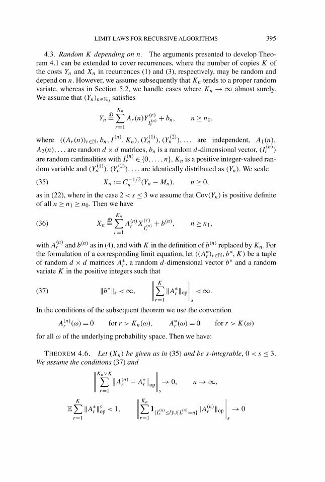
4.3. Random K depending on n. The arguments presented to develop Theo-rem 4.1 can be extended to cover recurrences, where the number of copies K ofthe costs Yn and Xn in recurrences (1) and (3), respectively, may be random anddepend on n. However, we assume subsequently that Kn tends to a proper randomvariate, whereas in Section 5.2, we handle cases where Kn → ∞ almost surely.We assume that (Yn)n∈N0 satisfies

YnD=

Kn∑r=1

Ar(n)Y(r)

I(n)r

+ bn, n ≥ n0,

where ((Ar(n))r∈N, bn, I(n)

,Kn), (Y(1)n ), (Y

(2)n ), . . . are independent, A1(n),

A2(n), . . . are random d × d matrices, bn is a random d-dimensional vector, (I(n)r )

are random cardinalities with I(n)r ∈ {0, . . . , n}, Kn is a positive integer-valued ran-

dom variable and (Y(1)n ), (Y

(2)n ), . . . are identically distributed as (Yn). We scale

Xn := C−1/2n (Yn − Mn), n ≥ 0,(35)

as in (22), where in the case 2 < s ≤ 3 we assume that Cov(Yn) is positive definiteof all n ≥ n1 ≥ n0. Then we have

XnD=

Kn∑r=1

A(n)r X

(r)

I(n)r

+ b(n), n ≥ n1,(36)

with A(n)r and b(n) as in (4), and with K in the definition of b(n) replaced by Kn. For

the formulation of a corresponding limit equation, let ((A∗r )r∈N, b∗,K) be a tuple

of random d × d matrices A∗r , a random d-dimensional vector b∗ and a random

variate K in the positive integers such that

‖b∗‖s < ∞,

∥∥∥∥∥K∑

r=1

‖A∗r ‖op

∥∥∥∥∥s

< ∞.(37)

In the conditions of the subsequent theorem we use the convention

A(n)r (ω) = 0 for r > Kn(ω), A∗

r (ω) = 0 for r > K(ω)

for all ω of the underlying probability space. Then we have:

THEOREM 4.6. Let (Xn) be given as in (35) and be s-integrable, 0 < s ≤ 3.We assume the conditions (37) and∥∥∥∥∥

Kn∨K∑r=1

∥∥A(n)r − A∗

r

∥∥op

∥∥∥∥∥s

→ 0, n → ∞,

E

K∑r=1

‖A∗r ‖s

op < 1,

∥∥∥∥∥Kn∑r=1

1{I (n)r ≤l}∪{I (n)

r =n}‖A(n)r ‖op

∥∥∥∥∥s

→ 0


for all l ∈ N. Then (Xn) converges to a limit X,

ζs(Xn,X) → 0, n → ∞,

where L(X) ∈ Mds (0, Idd) is given as the unique fixed point in Md

s (0, Idd) of theequation

XD=

K∑r=1

A∗rX

(r) + b∗.

Here (A∗1,A

∗2, . . . , b

∗,K),X(1),X(2), . . . are independent and X(r) ∼ X for r =1,2, . . . .

While we are mainly concerned with the analysis of combinatorial structures,data structures and recursive algorithms, where we typically have fixed K orKn → ∞ almost surely, the theorem may prove useful for the analysis of branchingprocesses such as Galton–Watson trees. In particular, the theorem covers a proofof Yaglom’s exponential limit law as given for an application of the contractionmethod in the �2 setting by Geiger [17]. The exponential limit distribution is

characterized as the fixed point of XD= U(X + X∗), with X,X∗,U independent

and U unif[0,1] distributed. The Kn is the number of children of the most recentcommon ancestor of the population at generation n.

5. Applications: central limit laws. In this section we link expansions ofmoments to our transfer theorem, Theorem 4.1, in a general setup. This leads toboth, asymptotic normality and nonnormal cases. The normal distribution appearsas the fixed point of the maps T given in (13) with

b = 0,

K∑r=1

ArAtr = Idd(38)

almost surely. It is easy to check by characteristic functions that N (0, Idd) isthen a fixed point of T and by Corollary 3.4 that this solution is unique in thespace Md

s (0, Idd) for s > 2 if E∑K

r=1 ‖Ar‖sop < 1. In all the central limit laws in

Section 5.3, the normal distribution as a limit distribution comes up as the fixedpoint of a transformation T satisfying (38).

We first focus on the univariate case d = 1 and link the expansion of themoments to our transfer theorem, Theorem 4.1, in a general setup that is notrestricted to normal limit distributions. This leads first to a general transfer theoremthat is capable of rederiving results involving nonnormal limit laws that alsocould be proven via the usage of �r metrics. We give some applications fromthe analysis of algorithms to illustrate our general theorem. Second, we give aconvenient specialization to asymptotic normality, which covers many examplesof central limit laws in the field of combinatorial structures. This is of particular


importance because the competitive �r metric approach does not lead to such atransfer theorem. In the last part we discuss the multivariate case together withexamples, where the number K of copies of the parameter on the right side maybe random, depend on n and satisfy Kn → ∞ almost surely.

5.1. Univariate central limit laws. A univariate situation quite common incombinatorial structures encompasses recursions of the type

YnD=

K∑r=1

Y(r)

I(n)r

+ bn, n ≥ n0,(39)

where (Y(1)n ), . . . , (Y

(K)n ), (I (n), bn) are independent, Y

(r)j ∼ Yj , j ≥ 0, P(I

(n)r =

n) → 0 for n → ∞ and r = 1, . . . ,K and such that Var(Yn) > 0 for n ≥ n1.Assume that for functions f,g : N0 → R

+0 with g(n) > 0 for n sufficiently large

we have the stabilization condition in Ls ,(g(I

(n)r )

g(n)

)1/2

→ A∗r , r = 1, . . . ,K,

(40)1

g1/2(n)

(bn − f (n) +

K∑r=1

f (I (n)r )

)→ b∗,

and the contraction condition

E

K∑r=1

(A∗r )

s < 1.(41)

THEOREM 5.1 (Univariate transfer theorem). Let (Yn) be s-integrable andsatisfy the recursive equation (39), and let f and g be given with stabilization andcontraction conditions (40) and (41) for some 0 < s ≤ 3. Assume

EYn ={

f (n) + o(g1/2(n)

), Var(Yn) = g(n) + o(g(n)), if 2 < s ≤ 3,

f (n) + o(g1/2(n)

), if 1 < s ≤ 2.

Then

Yn − f (n)

g1/2(n)

L→ X,

where X is the unique fixed point of

Xd=

K∑r=1

A∗rX

(r) + b∗(42)

in M1s (0,1), where (A∗

1, . . . ,A∗K,b∗),X(1), . . . ,X(K) are independent with

X(r) ∼ X.


PROOF. We denote Mn := EYn for 1 < s ≤ 3, Mn := f (n) for 0 < s ≤ 1,σn := √

Var(Yn) for 2 < s ≤ 3 and σn := √g(n) for 0 < s ≤ 2. First note that

(Yn − f (n))/g1/2(n)L→ X for some X if and only if Xn := (Yn − Mn)/σn

L→ X.We have

XnD=

K∑r=1

σI

(n)r

σn

XI

(n)r

+ 1

σn

(bn − Mn +

K∑r=1

MI

(n)r

), n ≥ n1.(43)

By (40) we obtain the following convergences in Ls :

limn→∞

σI

(n)r

σn

= limn→∞

(g(I

(n)r )

g(n)

)1/2

= A∗r , r = 1, . . . ,K,

limn→∞

1

σn

(bn − Mn +

K∑r=1

MI

(n)r

)

= limn→∞

1

g1/2(n)

(bn − f (n) +

K∑r=1

f (I (n)r )

)= b∗.

Furthermore, we have, for all l ≥ 0,

E

[1{I (n)

r ≤l}∪{I (n)r =n}

(I

(n)r

n

)s/2]

≤(

l

n

)s/2

+ P(I (n)r = n

)→ 0

for n → ∞. Since all the conditions of Theorem 4.1 are satisfied and X is theunique solution of

XD=

K∑r=1

A∗rX

(r) + b∗

in Mds (0,1) subject to (A1, . . . ,AK),X(1), . . . ,X(K) independent and X ∼ X(r)

for all r = 1, . . . ,K , the assertion follows. �

REMARK. Note that for s = 2 the order of the variance can be guessed fromconvergence in (40) and need not be known for the application of Theorem 5.1.Moreover, if the theorem can be applied for some g and s = 2, we obtain from theζ2 convergence in Theorem 4.1,

Var(Yn) = Var(X)g(n) + o(g(n))(44)

since h(x) := x2/2, x ∈ R, is in F2. Similarly if the theorem can be applied forsome f , g and s = 1, we obtain

EYn = E[X]g1/2(n) + f (n) + o(g1/2(n)

)(45)


since the identity map is in F1. The properties that the variance (or mean) can beguessed and proved by the application of the method are known for the �2 and �1metric approaches. From this point of view ζ2 and ζ1 are as powerful as �2 and �1,respectively. However, the range 2 < s ≤ 3 for ζs leads to applications especiallyincluding normal limit laws which are out of reach for the �p metrics for all p ≥ 1.

The case 0 < s ≤ 2 leads to examples which previously have been treated by the�p metrics. We first give some applications for these cases and focus then onthe range 2 < s ≤ 3, where we use the following specialization of Theorem 5.1for the application to normal limit laws, thus extending the previously knownframework of the contraction method.

COROLLARY 5.2 (Central limit theorem). Let (Yn) be s-integrable, s > 2, andsatisfy the recursive equation (39) with

EYn = f (n) + o(g1/2(n)

), Var(Yn) = g(n) + o(g(n)).

Assume for all r = 1, . . . ,K and some 2 < s ≤ 3,(

g(I(n)r )

g(n)

)1/2

→ A∗r ,

(46)1

g1/2(n)

(bn − f (n) +

K∑r=1

f (I (n)r )

)→ 0 in Ls

andK∑

r=1

(A∗r )

2 = 1, P(∃ r :A∗r = 1) < 1.(47)

Then

Yn − f (n)

g1/2(n)

L→ N (0,1),

where N (0,1) denotes the standard normal distribution.

PROOF. The conditions of the univariate transfer theorem, Theorem 5.1, aresatisfied with b∗ = 0. The solution of the fixed-point equation (42) in M1

s (0,1) isN (0,1) since

∑Kr=1(A

∗r )

2 = 1, b∗ = 0. �

In the following sections we give applications of Theorem 5.1 and Corollary 5.2for various choices of the parameters. We do not recall the underlying structures,for example, the various types of random graphs, but do introduce the essentialrecursive equations satisfied by the parameters of interest to cover the particularalgorithm or data structure. References to basic accounts on them are given.


5.2. Nonnormal limit laws.

Quickselect. The number of key comparisons Yn of the selection algorithmQuickselect, also known as FIND (for definition and mathematical analysis,see [18, 24, 32, 39]) when selecting the smallest order statistic in a set of n datasatisfies Y0 = Y1 = 0 and the recurrence

YnD= YIn + n − 1, n ≥ 2,

where (Yn) and In are independent with In unif{0, . . . , n − 1} distributed. Here,In corresponds to the size of the left sublist generated by the first splittingstep of the algorithm. We can directly apply Theorem 5.1 with K = 1, s = 1,f (n) = 0, g(n) = n2, I

(n)1 = In and bn = n − 1. We have (g(In)/g(n))1/2 → U

and bn/g1/2(n) → 1 in L1 for an appropriate unif[0,1] random variate U .

Condition (41) is satisfied because we have EU = 1/2 < 1. Hence we obtain

Yn

n

L−→ X, XD= UX + 1,(48)

where X and U are independent. This limit distribution is also known as theDickman distribution, which arises in number theory (see [56] and [24]). This caneasily be rederived by checking that the (shifted) Dickman distribution satisfies thefixed-point relationship (48).

For the case where we apply the Quickselect algorithm to select an order statisticof o(n) from a set of n data, we obtain the same limit distribution. This can bederived via a slight generalization of Theorem 5.1 and is as well covered withdifferent approaches by all four references given above.

COROLLARY 5.3. The normalized number of comparisons Yn/n of Quicks-elect when selecting an order statistic of o(n) from a set of n data converges indistribution to the (shifted) Dickman distribution given as the unique solution ofthe fixed point equation in (48).

Quicksort. The number of key comparisons Yn of the sorting algorithmQuicksort applied to a randomly permuted list of n numbers (see [35]) satisfiesY0 = Y1 = 0 and the recurrence

YnL= YIn + Y ∗

n−In+ n − 1, n ≥ 2,(49)

with (Yn), (Y ∗n ) and In independent and In unif{0, . . . , n− 1} distributed. It is well

known that EYn = 2n lnn + cn + o(n) for a constant c ∈ R. Theorem 5.1 can beapplied with K = 2, s = 2, f (n) = 2n lnn+cn, g(n) = n2, I (n)

1 = In, I (n)2 = n−In

and bn = n − 1. We have (g(In)/g(n))1/2 → U and (g(n − In)/g(n))1/2 →1 − U in L2 for an appropriate unif[0,1] random variate U . A direct calculation,


(see [48]) shows that

1

g1/2(n)

(bn − f (n) + f (In) + f (n − In)

)→ E(U)

= 1 + 2U ln(U) + 2(1 − U) ln(1 − U)

in L2. Condition (41) is satisfied because we have E[U2 + (1 − U)2] = 2/3 < 1.Thus Theorem 5.1 yields the convergence

Yn − 2n lnn − cn

n

L→ X ∈ M12(0,1), X

D= UX + (1 − U)X∗ + E(U),(50)

with X, X∗ and U independent and X ∼ X∗. This was first obtained by Rösler [48].

COROLLARY 5.4. The normalized number of comparisons (Yn − EYn)/n

of Quicksort when sorting a set of n randomly permuted data converges indistribution to the unique solution in M1

2(0,1) of the fixed point equation in (50).

This convergence holds as well in the ζ2 metric following from Theorem 4.1.Note that Corollaries 4.3 and 4.5 imply local and global convergence theoremsfor sequences (hn) tending to zero sufficiently slowly. The exact order of therate of convergence of the standardized cost of Quicksort for the ζ3 metric hasbeen identified to be of the order �(ln(n)/n); see [43]. Hence, on the basisof this refinement we obtain as well rates of convergence for global and localconvergences by applying Corollaries 4.3 and 4.5. This was made explicit byNeininger and Rüschendorf [43] for the case of Quicksort given in (49). Followingthis scheme, the general inequalities of Section 4.2 allow similar local and globalapproximation results for all the examples mentioned in Section 5.

Path length in m-ary search trees. The internal path length Yn of randomm-ary search trees, m ≥ 2, containing n data satisfies Yj = j for j = 0, . . . ,m − 1and

YnD=

m∑r=1

Y(r)

I(n)r

+ n − m + 1, n ≥ m,

with independence conditions as in recurrence (39). Let V = (U(1),U(2) −U(1), . . . ,1 − U(m−1)) denote the vector of spacings of independent unif[0,1]random variables U1, . . . ,Um−1. For u ∈ [0,1]m with

∑ur = 1 the conditional

distribution of I (n) given V = u is multinomial M(n − m + 1, u). It is knownthat EYn = (Hm − 1)−1n ln(n) + cmn + o(n) with constants cm ∈ R. We applyTheorem 5.1 with K = m, s = 2, f (n) = (Hm − 1)−1n ln(n) + cmn, g(n) = n2


and bn = n − m + 1. The conditional distribution of I (n) given V = u impliesI

(n)r /n → Vr in L2. A calculation similar to the Quicksort case (see [42]) yields

1

g1/2(n)

(bn − f (n) +

m∑r=1

f (I (n)r )

)→ 1 + 1

Hm − 1

m∑r=1

Vr ln(Vr).

Since E∑

V 2r < 1, we rederive a limit law from [42].

COROLLARY 5.5. The normalized internal path length (Yn − EYn)/n ofrandom m-ary search trees converges in distribution to the unique solution inM1

2(0,1) of the fixed point equation

XD=

m∑r=1

(VrX(r)) + 1 + 1

Hm − 1

m∑r=1

Vr ln(Vr),

with X(1), . . . ,X(m), V independent and X(r) ∼ X for r = 1, . . . ,m.

5.3. Normal limit laws.

5.3.1. Linear mean and variance.

Size of random m-ary search trees. The size Yn of the random m-ary searchtree (see [34]) containing n data satisfies Y0 = 0, Y1 = · · · = Ym−1 = 1 and therecursion

YnD=

m∑r=1

Y(r)

I(n)r

+ 1, n ≥ m.

Let V = (U(1),U(2) − U(1), . . . ,1 − U(m−1)) denote the vector of spacings ofindependent unif[0,1] random variables U1, . . . ,Um−1 as in the previous example.For u ∈ [0,1]m with

∑ur = 1 the conditional distribution of I (n) given V = u is

multinomial M(n − (m − 1), u). Thus we obtain

I (n)

n→ (

U(1),U(2) − U(1), . . . ,1 − U(m−1)

)(51)

in L1+ε. The mean and the variance satisfy, for 3 ≤ m ≤ 26 (see [2, 7, 31, 36]),

EYn = 1

2(Hm − 1)n + O(1 + nα−1), Var(Yn) = γmn + o(n),

with γm > 0 and α < 3/2 depending as well on m. Thus with Corollary 5.2 werederive the limit law (see [7, 33, 36]):

COROLLARY 5.6. The normalized size (Yn − EYn)/√

Var(Yn) of a randomm-ary search tree with 3 ≤ m ≤ 26 converges in distribution to the standardnormal distribution.


PROOF. We apply Corollary 5.2 with f (n) = (2(Hm − 1))−1n andg(n) = γmn. Condition (46) follows from (51); (47) holds since α < 3/2. �

The case of linear mean and variance is ubiquitous for parameters thatsatisfy (39), where the toll function bn is appropriately small. Such examplescovered by Corollary 5.2 are the number of certain patterns in random binarysearch trees, secondary cost parameters of Quicksort or the cost of certaintree traversal algorithms, Quicksort, m-ary search tree or generalized Quicksortrecursions with small toll functions; see [7, 8, 11, 12, 14, 16, 23].

5.3.2. Periodic functions in the mean and variance.

Size of random tries. The number Yn of internal nodes of a random trie withn keys in the symmetric Bernoulli model (see [34]) satisfies Y0 = 0 and

YnD= Y

(1)

I(n)1

+ Y(2)

I(n)2

+ 1, n ≥ 1,

where I(n)1 is B(n,1/2) distributed and I

(n)2 = n − I

(n)1 . The mean and variance

satisfy ([22])

EYn = n�1(log2 n) + O(1), Var(Yn) = n�2(log2 n) + O(1),(52)

where �1 and �2 are positive C∞ functions with period 1. We obtain a limit lawdue to Jacquet and Régnier [26]:

COROLLARY 5.7. The normalized size (Yn − EYn)/√

Var(Yn) of a randomtrie in the symmetric Bernoulli model converges in distribution to the standardnormal distribution.

PROOF. For the application of Corollary 5.2 we first check (47). We have

f (n) = n�1(log2 n), g(n) = n�2(log2 n),

where �1 and �2 are given in (52). Here and in the following discussion we usethe convention log2 n := 0 for n = 0. We split the sample space into the rangesA = {|I (n)

1 − n/2| < n3/4} and B = {|I (n)1 − n/2| ≥ n3/4}. Note that on A and B

also |I (n)2 − n/2| < n3/4 and |I (n)

2 − n/2| ≥ n3/4 hold, respectively.For the estimate on the set A we assume n to be sufficiently large so that

n−1/4 < 1/4. Then by the mean value theorem we obtain, for r = 1,2,

1 + log2I

(n)r

n= 1 + log2

(1

2+ I

(n)r − n/2

n

)= �n,r

I(n)r − n/2

n,(53)

where the random �n,r satisfy, on A,∥∥∥∥�n,r − 2

ln 2

∥∥∥∥∞≤ 8

ln 2n−1/4(54)


for n sufficiently large; in particular, |�n,r | ≤ 4/ ln 2, r = 1,2. Thus on A we have|1 + log2(I

(n)r /n)| ≤ (4/ ln 2)n−1/4, which implies, using the periodicity of �1,

�1(log2 I (n)r ) = �1

(log2 n +

(1 + log2

I(n)r

n

))(55)

= �1(log2 n) + �n,r

(1 + log2

I(n)r

n

)

with random

�n,r ∈{� ′

1(x + log2 n) : |x| ≤ 4

ln 2n−1/4

}=: Bn, r = 1,2.

By the continuity of � ′1 it follows that the sets Bn are intervals. Since � ′

1 is alsoperiodic, we obtain that � ′

1 is uniformly continuous and therefore the length of theintervals Bn tends to zero. This implies, on A,

‖�n,1 − �n,2‖∞ → 0, n → ∞.(56)

Now we verify condition (47) to apply Corollary 5.2. Combining (53) and (55) wehave, on A with n sufficiently large,

1√n

(I

(n)1 �1(log2 I

(n)1 ) + I

(n)2 �1(log2 I

(n)2 ) − n�1(log2 n)

)(57)

= 1√n

(�n,1�n,1I

(n)1

I(n)1 − n/2

n+ �n,2�n,2I

(n)2

I(n)2 − n/2

n

)(58)

= �n,1�n,11

n3/2

(I

(n)1

(I

(n)1 − n/2

)+ I(n)2

(I

(n)2 − n/2

))(59)

+ (�n,2�n,2 − �n,1�n,1)I

(n)2 (I

(n)2 − n/2)

n3/2 .(60)

First we estimate summand (60) on A. By (54) and (56) we have ‖�n,2�n,2 −�n,1�n,1‖∞ → 0; thus

∫A

∣∣∣∣(�n,2�n,2 − �n,1�n,1)I

(n)2 (I

(n)2 − n/2)

n3/2

∣∣∣∣3

dP

≤ ‖�n,2�n,2 − �n,1�n,1‖3∞∫ ∣∣∣∣I

(n)2 − n/2√

n

∣∣∣∣3

dP

= o(1)1

8E|N (0,1)|3 → 0, n → ∞.


For the first summand (59) we write I(n)1 /n = 1/2 + Rn, so that on A we have

‖Rn‖∞ ≤ n−1/4. Note that I(n)2 /n = 1/2 − Rn. This yields

1

n3/2

(I

(n)1

(I

(n)1 − n/2

)+ I(n)2

(I

(n)2 − n/2

))= 2Rn

I(n)1 − n/2√

n.

Since |�n,1�n,1| remains bounded, say bounded by C, we obtain∫A

∣∣∣∣�n,1�n,11

n3/2

(I

(n)1

(I

(n)1 − n/2

)+ I(n)2

(I

(n)2 − n/2

))∣∣∣∣3

dP

≤ 2C‖Rn‖3∞∫ ∣∣∣∣I

(n)1 − n/2√

n

∣∣∣∣3

dP → 0.

Putting this altogether, we obtain∫A

∣∣∣∣ 1

g1/2(n)

(1 − f (n) + f (I

(n)1 ) + f (I

(n)2 )

)∣∣∣∣3

dP → 0.

By Chernoff’s bound we have P(B) ≤ 2 exp(−√n ). With m2 :=

minx∈[0,1] �2(x) > 0 we obtain

∫B

∣∣∣∣∣I(n)r (�1(log2 I

(n)r ) − �1(log2 n))

g1/2(n)

∣∣∣∣∣3

dP

≤(

2‖�1‖∞m

1/22

)3

n3/22 exp(−√

n)→ 0

for r = 1,2, which implies∫B

∣∣∣∣ 1

g1/2(n)

(1 − f (n) + f (I

(n)1 ) + f (I

(n)2 )

)∣∣∣∣3

dP → 0.

Thus together we obtain (47).For (46) note that with g(n) := n�2(log2 n) we have

g(I(n)r )

g(n)= I

(n)r

n

�2(log2 I(n)r )

�2(log2 n).

By the strong law of large numbers (SLLN) and and dominated convergence,I

(n)r /n → 1/2 in any Lp . Furthermore

∣∣∣∣�2(log2 I(n)r )

�2(log2 n)− 1

∣∣∣∣=∣∣∣∣�2(log2(n) + 1 + log2(I

(n)r /n)) − �2(log2 n)

�2(log2 n)

∣∣∣∣≤ 1

m2

∣∣∣∣∣�2

(log2(n) + 1 + log2

(I

(n)r

n

))− �2(log2 n)

∣∣∣∣∣.


By the SLLN and the continuity of �2 this tends to zero almost surely. Bydominated convergence, the convergence holds in any Lp . Together this implies

g(I(n)r )

g(n)→ 1

2, in Ls

for any s > 0. �

REMARK. Note that the properties of �1 and �2 that are needed are theperiodicity, the lower positive bound for �2, that �1 is continuously differentiableand that �2 is continuous. This seems to be of some generality as the followingexamples on path lengths in digital structures show. However, there are alsoexamples where the differentiability of �1 fails to hold and our method still maybe applied as shown below for the top-down mergesort.

Path lengths in digital structures. The fundamental search trees based on bitcomparisons are the digital search tree, the trie and the Patricia trie; see [55]. Thecost to build up these trees from n data is measured by their path lengths Yn, thatis, the internal path length for digital search trees and the external path lengths fortries and Patricia tries. In the symmetric Bernoulli model we have Y0 = 0 and

YnD= Y

(1)

I(n)1

+ Y(2)

I(n)2

+ n − bn, n ≥ 1,

where I(n)1 ∼ B(n − 1,1/2), I

(n)1 + I

(n)2 = n − 1 and bn = 1 for digital search

trees, and for the other two structures, I (n)1 ∼ B(n,1/2), I (n)

1 +I(n)2 = n and bn = 0

for the trie and bn = 1{I (n)1 ∈{0,n}}n for Patricia tries. The small disturbance in the

recursion is reflected by their similar moments,

EYn = n log2 n + n�3(log2 n) + O(log n),

VarYn = n�4(log2 n) + O(log2 n),

where �r are periodic functions (with period 1) that vary from one of the structuresto the other; see [28–31]. It is known that �4 is continuous and positive in eachcase. For �3 we have the representations

�3(x) = C + 1

ln 2

∑k∈Z\{0}

(−ωk)e2kπix, x ∈ R,

for the digital search tree and

�3(x) = C + 1

ln 2

∑k∈Z\{0}

ωk(−ωk)e2kπix, x ∈ R,

for the trie and Patricia trie, where the constant C varies from case to case and

ωk = 1 + 2kπi

ln 2, k ∈ Z.


Note that for Fourier series h(x) =∑k∈Z ake

2πikx the condition |ak| = O(k−(m+2))

for |k| → ∞ implies that h is m times continuously differentiable. Since |(−ωk)|decays exponentially for |k| → ∞, we obtain that �3 is infinite differentiable in allcases. Only the C1 property is needed. This implies asymptotic normality, whichfor digital search trees and tries was proven in [25] and [27], respectively; seealso [52]:

COROLLARY 5.8. The normalized internal (resp., external) path lengths(Yn − EYn)/

√Var(Yn) of digital search trees, tries and Patricia tries are

asymptotically normal in the symmetric Bernoulli model.

PROOF. We apply Corollary 5.2. Condition (46) follows from the continuityof �4 as in the proof of Corollary 5.7. For (47) we have

1√n

(n − bn − n log2 n − n�3(log2 n) + I

(n)1 log2 I

(n)1

+ I(n)1 �3(log2 I

(n)1 ) + I

(n)2 log2 I

(n)2 + I

(n)2 �3(log2 I

(n)2 )

)= − bn√

n+ 1√

n

(n + I

(n)1 log2 I

(n)1 + I

(n)2 log2 I

(n)2 − n log2 n

)(61)

+ 1√n

(I

(n)1 �3(log2 I

(n)1 ) + I

(n)2 �3(log2 I

(n)2 ) − n�3(log2 n)

).(62)

Now, bn/√

n tends to zero in Lp for any p > 0 in all three cases. The summandin (62) is essentially the term (57) estimated in the proof of Corollary 5.7. Thesecond summand in (61) can also be seen to tend to zero in L3 by the estimatesof Corollary 5.7: Applying (53) leads to (58) with �n,1 = �n,2 = 1 there; thus wecan conclude as in Corollary 5.7. �

For related recursions that arise in the analysis of the size and path length ofbucket digital search trees, see [19].

Mergesort. The number of key comparisons Yn of top-down mergesort (fordefinition and mathematical analysis, see [15] and [20]), applied to a list ofn randomly permuted items, satisfies Y0 = 0 and

YnD= Y

(1)

I(n)1

+ Y(2)

I(n)2

+ n − Sn, n ≥ 1,

where I(n)1 = �n/2�, I (n)

2 = n− I(n)1 and Sn is a random variate that is independent

of (Y(1)n ) and (Y

(2)n ); see [31], Section 5.2.4. In particular, we have ES3

n = O(1).Flajolet and Golin [15] proved

EYn = n log2 n + n�5(log2 n) + O(1),(63)

Var(Yn) = n�6(log2 n) + o(n),


where �5 and �6 are continuous functions with period 1, �6 is positive and �5is not differentiable. In particular,

�5(u) = C + 1

ln 2

∑k∈Z\{0}

1 + �(χk)

χk(χk + 1)e2kπiu, u ∈ R,(64)

where C ∈ R is a constant, � is a complex function of O(1) on the imaginary line�(s) = 0 and

χk = 2πik

ln 2, k ∈ Z.

Moreover, Flajolet and Golin showed that (Yn −EYn)/√

Var(Yn) satisfies a centrallimit theorem by applying Lyapunov’s condition. Hwang [20] found a local limittheorem and large deviations including rates of convergence and, in [21], gavefull (exact) asymptotic expansions for the mean and variance. Cramer [9] obtainedthe (central) limit law by applying the contraction method. For methodologicalreasons, we rederive this limit law on the basis of the expansions (63) includingthe representation for �5 directly from Corollary 5.2: We have

f (n) = n log2(n) + n�5(log2 n), g(n) = n�6(log2 n).

Thus, by I(n)1 = �n/2� and the continuity of �6, we have deterministically

(g(I

(n)1 )

g(n)

)1/2

→ 1√2,

(g(I

(n)2 )

g(n)

)1/2

→ 1√2.

Since ES3n = O(1) we obtain, in L3,

1√n

(f (I

(n)1 ) + f (I

(n)2 ) − f (n) + n − Sn

)

= 1√n

(⌈n

2

⌉log2

⌈n

2

⌉+(n −

⌈n

2

⌉)log2

(n −

⌈n

2

⌉)(65)

− n log2(n) +⌈

n

2

⌉�5

(log2

⌈n

2

⌉)

+(n−

⌈n

2

⌉)�5

(log2

(n −

⌈n

2

⌉))− n�5(log2 n) + n − Sn

)

→ 0,

where the only nontrivial contribution comes from the �5 terms in (65) with odd n,say n = 2m + 1. The asymptotic cancellation of these terms follows from∣∣�5

(log2(m + 1)

)− �5(log2(m + 1/2)

)∣∣= o(m−1/2).


For this note that∣∣∣∣exp(2kπi log2(m + 1)

)− exp(

2kπi log2

(m + 1

2

))∣∣∣∣≤ min

{2,

πk

(m + 1/2) ln(2)

}, k ∈ Z, m ∈ N,

and that ∣∣∣∣ 1 + �(χk)

χk(χk + 1)

∣∣∣∣≤ c

k2 , k ∈ Z \ {0},

with a constant c > 0. Now we split the range of summation in (64) into the ranges|k| ≤ m and |k| > m and note that

∑k>m k−2 = O(1/m). This yields∣∣∣∣�5

(log2(m + 1)

)− �5

(log2

(m + 1

2

))∣∣∣∣= O

(Hm

m

).

COROLLARY 5.9. The normalized number of key comparisons (Yn − EYn)/√Var(Yn) of top-down mergesort applied to a randomly permuted number of items

is asymptotically normal.

For other variants of mergesort and a limit law for the queue mergesort, see [6]and the references therein. Note that the limit law for queue mergesort in [6] cannotbe obtained by Corollary 5.2 since the corresponding prefactors (g(I

(n)r )/g(n))1/2

do not converge, r = 1,2. However, the extension of our approach in Section 5.2seems to be promising.

5.3.3. Other orders for mean and variance.

Maxima in right triangles. We consider the number Yn of maxima of n

independent, uniform samples in a right triangle in R2 with vertices (0,0), (1,0)

and (0,1); see [3] and [4]. According to Proposition 1 in [3], this number satisfiesthe recursion Y0 = 0 and

YnD= Y

(1)

I(n)1

+ Y(2)

I(n)2

+ 1,

where the indices I(n)1 and I

(n)2 are given as the first two components of a mixed

trinomial distribution as follows: Let (Un,Vn) denote the point that maximizes thesum of the components in the sample of the n points. Then I (n) = (I

(n)1 , I

(n)2 , I

(n)3 )

conditioned on (Un,Vn) = (u, v) is multinomially distributed:

PI (n)|(Un,Vn)=(u,v) = M

(n − 1,

u2

(u + v)2,

v2

(u + v)2,

2uv

(u + v)2

).


The mean and variance satisfy (see [3])

EYn = √π

√n + O(1),

Var(Yn) = σ 2√n + O(1),

with some σ 2 > 0. Thus we have the orders f (n) = √π

√n and g(n) = σ 2√n.

Moreover, I (n)/n → (U2, (1 −U)2,2U), where U is unif[0,1] distributed. So weobtain I

(n)1 /n → U1/2 and I

(n)2 /n → (1 − U)1/2 in any Lp . In [4] by the method

of moments, a central limit law for Yn was derived. We can give an easy approachto asymptotic normality based on Corollary 5.2:

COROLLARY 5.10. Let Yn be the number of maxima of n independent uniformsamples in a right triangle as described above. Then

Yn − EYn√Var(Yn)

L→ N (0,1).

PROOF. It remains to check (46). We have

1

n1/4

∣∣(I (n)1 )1/2 + (I

(n)2 )1/2 − n1/2∣∣

≤ n1/4∣∣∣∣(

I(n)1

n − 1

)1/2

− Un

Un + Vn

∣∣∣∣+ n1/4∣∣∣∣(

I(n)2

n − 1

)1/2

− Vn

Un + Vn

∣∣∣∣+ O(n−3/4).

It is sufficient to bound one of these two nontrivial summands. We denote

A :={(

I(n)1

n − 1

)1/2

+ Un

Un + Vn

≥ n−3/14},

B :={(

I(n)1

n − 1

)1/2

+ Un

Un + Vn

< n−3/14}.

On A it holds that∣∣∣∣(

I(n)1

n − 1

)1/2

− Un

Un + Vn

∣∣∣∣3

≤ n9/14∣∣∣∣ I

(n)1

n − 1− U2

n

(Un + Vn)2

∣∣∣∣3

.

Thus denoting by ϒn the distribution of U2n/(Un + Vn)

2 and denoting by Bn,u aB(n − 1, u) distributed random variable, we obtain

∫A

∣∣∣∣(

I(n)1

n − 1

)1/2

− Un

Un + Vn

∣∣∣∣3

dP ≤ n9/14∫ ∣∣∣∣ Bn,u

n − 1− u

∣∣∣∣3

dϒn(u)

≤ n9/14Cn−3/2 = Cn−6/7,


since the third absolute central moment of Bn,u is bounded by Cn3/2 with aconstant C > 0 uniformly in p ∈ [0,1], following from Chernoff’s bound. On B

we use the trivial bound∫B

∣∣∣∣(

I(n)1

n − 1

)1/2

− Un

Un + Vn

∣∣∣∣3

dP ≤ P(B)n−9/14.

Finally we obtain, with ϒ ′n denoting the distribution of Un + Vn,

P(B) = P

(Un

Un + Vn

≤ n−3/14)

= P

(Un

Un + Vn

≤ n−3/14,0 ≤ Un + Vn ≤ 1

2

)

+ P

(Un

Un + Vn

≤ n−3/14,1

2≤ Un + Vn ≤ 1

)

≤(

1

4

)n

+ P

(Un ≤ n−3/14,Un + Vn ≥ 1

2

)

=(

1

4

)n

+∫ 1

1/2

√2n−3/14√

2udϒ ′

n(u)

= O(n−3/14).

Thus putting everything altogether, we obtain∥∥∥∥ 1

g1/2(n)

(f (n) − f (I

(n)1 ) − f (I

(n)2 )

)∥∥∥∥3(66)

= O((n3/4n−6/7)1/3)= O(n−1/28).

The assertion follows by Corollary 5.2. �

Note that estimates for the term (66) are also required in the moments methodapproach in [3]; compare the (different) estimates of Vr(n) there on pages14 and 15.

5.4. Multivariate central limit laws. The generalization of Corollary 5.2 tohigher dimensions is straightforward and is omitted here. Applications of suchan extension cover, for example, limit laws for recursions as in [33]. Instead, weextend our approach to multivariate recursions where the number K of copiesof the parameter on the right side may be random, depending on n, and evensatisfy K = Kn → ∞ for n → ∞. Clearly, in such a situation the heuristicthat a stabilization of the coefficients as in (24) plus a contraction condition asin (25) leads to a fixed-point equation and a related convergence theorem as in


Theorem 4.1 no longer holds. However, for normal convergence problems, we usethe fact that the multivariate standard normal distribution satisfies all the equations

XD=

Kn∑r=1

ArX(r)(67)

with (Kn,A1,A2, . . .),X(1),X(2), . . . independent, X ∼ X(r) for all r ≥ 1 and∑Kn

r=1 ArAtr = Idd . For problems with Kn → ∞, we typically have Ar tending to

zero for n → ∞ for every fixed r , so that we have no meaningful limiting equationat hand. Nevertheless, our arguments may apply, since we are able to compare witha normal distribution for every n by means of an (in n changing) equation of thetype (67).

5.4.1. Random recursive trees. The recursive tree of order n is a rooted tree onn vertices labeled 1 to n such that for each k = 2, . . . , n, the labels of the verticeson the path from the root to the node labeled k form an increasing sequence. Fora random recursive tree of order n, we assume the uniform model on the space ofall recursive trees of order n, where all (n − 1)! trees are equally likely. It is wellknown that a random recursive tree may be obtained by successively adjoiningchildren to the existing tree, where for the nth vertex the parent node is chosenuniformly from the vertices labeled 1, . . . , n − 1. For a survey of recursive trees,we refer to [54]. Mahmoud and Smythe [38] studied the joint distribution of Yn =(Bn,Rn,Gn), where Bn, Rn and Gn are the number of vertices in the tree without-degree 0, 1 and 2, respectively. Based on a formulation as a generalized Pólya–Eggenberger urn model, they derived the mean EYn = n(1/2,1/4,1/8) + O(1)

and the covariance matrix Cov(Yn) = n�0 + O(1), where �0 is explicitly givenin [38], Theorem 4.1. By an application of a martingale central limit theorem, theasymptotic trivariate normality is shown.

Here, we offer a recursive approach to parameters of random recursive treesbased on a generalization of our previous settings, allowing the number K ofsummands on the right-hand side of (1) to be random, depending on n, and tendingto infinity for n → ∞.

There are several possibilities for a recursive decomposition of a parameterof a random recursive tree: First of all we may decompose by counting theparameters of all the Kn subtrees separately and calculate from these the parameterof the whole tree. This is the line we follow in the subsequent analysis. Herethe random number Kn of subtrees of the root has a representation as a sum ofindependent Bernoulli random variables. Second, we could also subdivide into,for example, the leftist subtree of the root and the rest of the tree (including theroot) as was done in [13] for the analysis of the internal path length in randomrecursive trees. However, the example of Mahmoud and Smythe [38] will, inthis decomposition, not be covered by our present approach, since a dependencebetween bn and (Y

(2)n ) is present which is forbidden in our setup. Third, we


may first use a bijection between recursive trees and binary search trees, the“oldestchildnextsibling” (see [1]), transpose the parameter under considerationinto the binary search tree setting and use the recursive structure of the binarysearch tree. However, parameters of a simple form for recursive trees may havemore complex counterparts in the binary search tree setup.

The vector Yn defined above satisfies the recursions Y0 = (0,0,0), Y1 = (1,0,0)

and

YnD=

Kn∑r=1

Y(r)

I(n)r

+ bn, n ≥ n0,(68)

with n0 = 2 and bn = (1{Kn=0},1{Kn=1},1{Kn=2}), where (Kn, I(n), bn), (Y

(1)n ),

(Y(2)n ), . . . are independent with Y

(r)j ∼ Yj for all j ≥ 0, r ≥ 1. Here, we use that

given the number Kn and the cardinalities I(n)1 , . . . , I

(n)Kn

of the subtrees of the root,

these subtrees are random recursive trees of orders I(n)1 , . . . , I

(n)Kn

, respectively, andare independent of each other.

More generally, we assume that (Yn) is a sequence of random d-dimensionalvectors satisfying (68), where bn is “small”; more precisely, bn/

√n → 0 in L3,

and mean and (co)variances of Yn are linear, that is,

EYn = nµ + o(√

n), Cov(Yn) = n� + o(n),(69)

with components µl �= 0 for l = 1, . . . , d and � being positive definite. We assumeCov(Yn) to be positive definite for some n ≥ n1 and scale as in (22) with 2 < s ≤ 3,Xn := C

−1/2n (Yn − Mn). This leads to the recursion

XnD=

Kn∑r=1

A(n)r X

(r)

I(n)r

+ b(n), n ≥ n1,(70)

with

A(n)r =

(I

(n)r

n

)1/2

Idd +o(1), b(n) = o(1),(71)

where the o(1) terms are converging uniformly. A substitute for the contractioncondition (25) is given by the next lemma:

LEMMA 5.11. Let Kn be the out-degree of the root of a random recursive treeof order n and let I

(n)1 , . . . , I

(n)Kn

be the cardinalities of the subtrees of the root.Then, for all s > 2,

lim supn→∞

E

Kn∑r=1

(I

(n)r

n

)s/2

≤ 6 + s

4 + 2s< 1

holds.


PROOF. By Theorem 5.1 in [37] we have, in particular, I(n)1 /n → U ∼

unif[0,1] almost surely. Hence it follows that

E

Kn∑r=1

(I

(n)r

n

)s/2

≤ E

[(I

(n)1

n

)s/2

+Kn∑r=2

I(n)r

n

](72)

= E

[(I

(n)1

n

)s/2

+ n − 1 − I(n)1

n

]

→ 6 + s

4 + 2s, n → ∞.

The assertion follows. �

COROLLARY 5.12. Let (Yn) be a sequence of vectors of parameters of arandom recursive tree in L3 satisfying (68) and (69). Then, for all 2 < s ≤ 3,

ζs

(Cov(Yn)

−1/2(Yn − EYn),N (0, Idd))→ 0, n → ∞,

holds.

PROOF. For an estimate as in the proof of Theorem 4.1, we introduce theaccompanying sequence

QnD=

Kn∑r=1

A(n)r

(1{I (n)

r <n1}X(r)

I(n)r

+ 1{I (n)r ≥n1}N

(r))

+ b(n), n ≥ 2,

where (A(n)1 , . . . ,A

(n)Kn

, b(n), I (n),Kn),N(1),N(2), . . . , (X

(1)n ), (X

(2)n ), . . . are inde-

pendent with N(r) ∼ N (0, Idd), X(r)j ∼ Xj for r ≥ 1, 0 ≤ j < n1 − 1. Then we

have

ζs

(Xn,N (0, Idd)

)≤ ζs(Xn,Qn) + ζs

(Qn,N (0, Idd)

).

As in the proof of Theorem 4.1, we obtain [cf. (33)]

ζs(Xn,Qn) ≤∫ ∫ k∑

r=1

1{jr≥n1}‖αr‖sopζs(Xjr ,X)dϒ(k)

n (α, j) dPKn(k),(73)

where ϒ(k)n is the joint distribution of (A

(n)1 , . . . ,A

(n)Km

, I (n)) given Kn = k andα = (α1, . . . , αk), j = (j1, . . . , jk). This implies

ζs

(Xn,N (0, Idd)

)≤(

E

Kn∑r=1

‖A(n)r ‖s

op

)sup

n1≤j≤n−1ζs

(Xj ,N (0, Idd)

)+ o(1).(74)

By (71) and Lemma 5.11 the prefactor is less than or equal to (6 + s)/(4 + 2s) < 1


for n sufficiently large, which gives that (ζ(Xn,N (0, Idd))) is bounded. Thenwith ξ := lim sup ζ(Xn,N (0, Idd)), we obtain from (73), as in the proof ofTheorem 4.1,

ξ ≤ 6 + s

4 + 2s(ξ + ε)

for all ε > 0; thus ξ = 0. �

As a consequence we obtain, in particular, the asymptotic trivariate normalityresult of Mahmoud and Smythe [38].

5.4.2. Random plane-oriented recursive trees. Plane-oriented recursive treesare recursive trees with ordered sets of descendents; a random plane-orientedrecursive tree of order n is chosen with equal probability from the space of allsuch trees, with n nodes. As for random recursive trees, there is a probabilisticgrowth rule available to build up the plane-oriented counterpart; for details anddefinitions, see [54].

Parameters of random recursive trees which admit a representation (68) havecounterparts for plane-oriented recursive trees, where (68) is still valid, butthe distribution of (Kn, I

(n)) has to be adjusted. These two trees behave quitedifferently. For example, the growth order of the number of subtrees Kn of theroot, on the average, changes from being logarithmic to

√n when switching to the

plane-oriented version. A convergence scheme similar to Corollary 5.12 can bebuilt upon the following contraction lemma, which corresponds to Lemma 5.11:

LEMMA 5.13. Let Kn be the out-degree of the root of a random plane-oriented recursive tree of order n and let I

(n)1 , . . . , I

(n)Kn

be the cardinalities of thesubtrees of the root. Then, for all s > 2,

lim supn→∞

E

Kn∑r=1

(I

(n)r

n

)s/2

≤ 5 + 2s

3 + 3s< 1

holds.

PROOF. We enumerate the subtrees of the root such that the first subtree inour enumeration is the one with root labeled 2. Then by Theorem 5 in [40],I (n)/n → V holds almost surely, where V has the beta(1/2,1) distribution. Inparticular, EV s/2 = 1/(s + 1) for s > 0. An estimate similar to (72) leads to theassertion. �

From this contraction property we obtain that our Corollary 5.12 is valid alsofor the plane-oriented version of the recursive tree.


COROLLARY 5.14. Let (Yn) denote the vector of parameters of plane-oriented recursive trees in L3 that satisfy (68) and (69). Then

ζs

(Cov(Yn)

−1/2(Yn − EYn),N (0, Idd))→ 0, n → ∞.

For possible applications, see Section 8 in [40].

Acknowledgments. We thank Hsien-Kuei Hwang for pointing out some ofthe applications in Section 5. The referee’s comments are very much appreciated.

REFERENCES

[1] AHO, A. V., HOPCROFT, J. E. and ULLMAN, J. D. (1983). Data Structures and Algorithms.Addison–Wesley, Reading, MA.

[2] BAEZA-YATES, R. A. (1987). Some average measures in m-ary search trees. Inform. Process.Lett. 25 375–381.

[3] BAI, Z.-D., HWANG, H.-K., LIANG, W.-Q. and TSAI, T.-H. (2001). Limit theorems for thenumber of maxima in random samples from planar regions. Electron. J. Probab. 6.

[4] BAI, Z.-D., HWANG, H.-K. and TSAI, T.-H. (2002). Berry–Esseen bounds for the number ofmaxima in planar regions. Electron J. Probab. 8.

[5] BURTON, R. and RÖSLER, U. (1995). An L2 convergence theorem for random affinemappings. J. Appl. Probab. 32 183–192.

[6] CHEN, W.-M., HWANG, H.-K. and CHEN, G.-H. (1999). The cost distribution of queue-mergesort, optimal mergesorts, and power-of-2 rules. J. Algorithms 30 423–448.

[7] CHERN, H.-H. and HWANG, H.-K. (2001). Phase changes in random m-ary search trees andgeneralized quicksort. Random Structures Algorithms 19 316–358.

[8] CHERN, H.-H., HWANG, H.-K. and TSAI, T.-H. (2002). An asymptotic theory for Cauchy–Euler differential equations with applications to the analysis of algorithms. J. Algorithms44 177–225.

[9] CRAMER, M. (1997). Stochastic analysis of the merge–sort algorithm. Random StructuresAlgorithms 11 81–96.

[10] CRAMER, M. and RÜSCHENDORF, L. (1995). Analysis of recursive algorithms by thecontraction method. Athens Conference on Applied Probability and Time Series Analysis.Lecture Notes in Statist. 114 18–33. Springer, New York.

[11] DEVROYE, L. (1991). Limit laws for local counters in random binary search trees. RandomStructures Algorithms 2 303–315.

[12] DEVROYE, L. (2003). Limit laws for sums of functions of subtrees of random binary searchtrees. SIAM J. Comput. 32 152–171.

[13] DOBROW, R. P. and FILL, J. A. (1999). Total path length for random recursive trees. Combin.Probab. Comput. 8 317–333.

[14] FILL, J. A. (1996). On the distribution of binary search trees under the random permutationmodel. Random Structures Algorithms 8 1–25.

[15] FLAJOLET, P. and GOLIN, M. (1994). Mellin transforms and asymptotics. The mergesortrecurrence. Acta Inform. 31 673–696.

[16] FLAJOLET, P., GOURDON, X. and MARTÍNEZ, C. (1997). Patterns in random binary searchtrees. Random Structures Algorithms 11 223–244.

[17] GEIGER, J. (2000). A new proof of Yaglom’s exponential limit law. In Algorithms, TreesCombinatorics and Probability (D. Gardy and A. Mokkadem, eds.) 245–249. Birkhäuser,Basel.


[18] GRÜBEL, R. and RÖSLER, U. (1996). Asymptotic distribution theory for Hoare’s selectionalgorithm. Adv. in Appl. Probab. 28 252–269.

[19] HUBALEK, F., HWANG, H.-K., LEW, W., MAHMOUD, H. M. and PRODINGER, H. (2002).A multivariate view of random bucket digital search trees. J. Algorithms 44 121–158.

[20] HWANG, H.-K. (1996). Asymptotic expansions of the mergesort recurrences. Acta Inform. 35911–919.

[21] HWANG, H.-K. (1998). Limit theorems for mergesort. Random Structures Algorithms 8319–336.

[22] HWANG, H.-K. (2001). Lectures on asymptotic analysis given at McGill Univ., Montreal.[23] HWANG, H.-K. and NEININGER, R. (2002). Phase change of limit laws in the quicksort

recurrence under varying toll functions. SIAM J. Comput. 31 1687–1722.[24] HWANG, H.-K. and TSAI, T.-H. (2002). Quickselect and Dickman function. Combin. Probab.

Comput. 11 353–371.[25] JACQUET, P. and RÉGNIER, M. (1988). Normal limiting distribution of the size and the external

path length of tries. Technical Report RR-0827, INRIA-Rocquencourt.[26] JACQUET, P. and RÉGNIER, M. (1988). Normal limiting distribution of the size of tries. In

Performance’87 209–223. North-Holland, Amsterdam.[27] JACQUET, P. and SZPANKOWSKI, W. (1995). Asymptotic behavior of the Lempel–Ziv parsing

scheme and digital search trees. Theoret. Comput. Sci. 144 161–197.[28] KIRSCHENHOFER, P., PRODINGER, H. and SZPANKOWSKI, W. (1989). On the balance

property of Patricia tries: External path length viewpoint. Theoret. Comput. Sci. 68 1–17.[29] KIRSCHENHOFER, P., PRODINGER, H. and SZPANKOWSKI, W. (1989). On the variance of

the external path length in a symmetric digital trie. Discrete Appl. Math. 25 129–143.[30] KIRSCHENHOFER, P., PRODINGER, H. and SZPANKOWSKI, W. (1994). Digital search trees

again revisited: The internal path length perspective. SIAM J. Comput. 23 598–616.[31] KNUTH, D. E. (1973). The Art of Computer Programming 3. Addison–Wesley, Reading, MA.[32] KODAJ, B. and MÓRI, T. F. (1997). On the number of comparisons in Hoare’s algorithm

“FIND.” Studia Sci. Math. Hungar. 33 185–207.[33] LEW, W. and MAHMOUD, H. M. (1994). The joint distribution of elastic buckets in multiway

search trees. SIAM J. Comput. 23 1050–1074.[34] MAHMOUD, H. M. (1992). Evolution of Random Search Trees. Wiley, New York.[35] MAHMOUD, H. M. (2000). Sorting. A Distribution Theory. Wiley, New York.[36] MAHMOUD, H. M. and PITTEL, B. (1989). Analysis of the space of search trees under the

random insertion algorithm. J. Algorithms 10 52–75.[37] MAHMOUD, H. M. and SMYTHE, R. T. (1991). On the distribution of leaves in rooted subtrees

of recursive trees. Ann. Appl. Probab. 1 406–418.[38] MAHMOUD, H. M. and SMYTHE, R. T. (1992). Asymptotic joint normality of outdegrees of

nodes in random recursive trees. Random Structures Algorithms 3 255–266.[39] MAHMOUD, H. M., MODARRES, R. and SMYTHE, R. T. (1995). Analysis of quickselect: An

algorithm for order statistics. RAIRO Inform. Théor. Appl. 29 255–276.[40] MAHMOUD, H. M., SMYTHE, R. T. and SZYMANSKI, J. (1993). On the structure of

random plane-oriented recursive trees and their branches. Random Structures Algorithms4 151–176.

[41] NEININGER, R. (2001). On a multivariate contraction method for random recursive structureswith applications to Quicksort. Random Structures Algorithms 19 498–524.

[42] NEININGER, R. and RÜSCHENDORF, L. (1999). On the internal path length of d-dimensionalquad trees. Random Structures Algorithms 15 25–41.

[43] NEININGER, R. and RÜSCHENDORF, L. (2002). Rates of convergence for Quicksort.J. Algorithms 44 52–62.


[44] PITTEL, B. (1999). Normal convergence problem? Two moments and a recurrence may be theclues. Ann. Appl. Probab. 9 1260–1302.

[45] RACHEV, S. T. (1991). Probability Metrics and the Stability of Stochastic Models. Wiley, NewYork.

[46] RACHEV, S. T. and RÜSCHENDORF, L. (1994). On the rate of convergence in the CLTwith respect to the Kantorovich metric. In Probability in Banach Spaces (J. Hoffmann-Jorgensen, J. Kuelbs and M. B. Marcus, eds.) 9 193–207. Birkhäuser, Boston.

[47] RACHEV, S. T. and RÜSCHENDORF, L. (1995). Probability metrics and recursive algorithms.Adv. in Appl. Probab. 27 770–799.

[48] RÖSLER, U. (1991). A limit theorem for “Quicksort.” RAIRO Inform. Théor. Appl. 25 85–100.[49] RÖSLER, U. (1992). A fixed point theorem for distributions. Stochastic Process. Appl. 42

195–214.[50] RÖSLER, U. (2001). On the analysis of stochastic divide and conquer algorithms. Algorithmica

29 238–261.[51] RÖSLER, U. and RÜSCHENDORF, L. (2001). The contraction method for recursive algorithms.

Algorithmica 29 3–33.[52] SCHACHINGER, W. (2001). Asymptotic normality of recursive algorithms via martingale

difference arrays. Discrete Math. Theor. Comput. Sci. 4 363–397.[53] SENATOV, V. V. (1980). Some uniform estimates of the convergence rate in the multidimen-

sional central limit theorem. Theory Probab. Appl. 25 745–759.[54] SMYTHE, R. T. and MAHMOUD, H. M. (1994). A survey of recursive trees. Teor. Imovır. ta

Mat. Statist. 51 1–29.[55] SZPANKOWSKI, W. (2001). Average Case Analysis of Algorithms on Sequences. Wiley, New

York.[56] TENENBAUM, G. (1995). Introduction to Analytic and Probabilistic Number Theory.

(C. B. Thomas, transl.). Cambridge Univ. Press.[57] ZOLOTAREV, V. M. (1976). Approximation of the distributions of sums of independent random

variables with values in infinite-dimensional spaces. Theory Probab. Appl. 21 721–737.[58] ZOLOTAREV, V. M. (1977). Ideal metrics in the problem of approximating distributions of

sums of independent random variables. Theory Probab. Appl. 22 433–449.

SCHOOL OF COMPUTER SCIENCE

MCGILL UNIVERSITY

3480 UNIVERSITY STREET

MONTREAL

CANADA H3A 2K6E-MAIL: [email protected]

INSTITUT FÜR MATHEMATISCHE STOCHASTIK

UNIVERSITÄT FREIBURG

ECKERSTRASSE 179104 FREIBURG

GERMANY

E-MAIL: [email protected]

A GENERAL LIMIT THEOREM FOR ... - math.uni-frankfurt.deneiningr/asynorm.pdf · LIMIT LAWS FOR...

Documents

Transcript of A GENERAL LIMIT THEOREM FOR ... - math.uni-frankfurt.deneiningr/asynorm.pdf · LIMIT LAWS FOR...