
A General Equilibrium Model of Supply Chain...
29
A General Equilibrium Model of Supply Chain Interactions and Risk Propagation John Birge and Jing Wu 1 1 University of Chicago Booth School of Business SCF Symposium, Madrid John Birge and Jing Wu (Chicago Booth) Equilibrium in Supply Chain Networks June 20, 2016 1 / 29
Transcript of A General Equilibrium Model of Supply Chain...

A General Equilibrium Model of Supply ChainInteractions and Risk Propagation
John Birge and Jing Wu1
1University of Chicago Booth School of Business
SCF Symposium, Madrid
John Birge and Jing Wu (Chicago Booth) Equilibrium in Supply Chain Networks June 20, 2016 1 / 29

S&P 500 Supply Chain Network
ADI
A
ANSS
FLEX
JBL
NTAP
SNPS
XLNX
CSC
AA
CSX
FLR
ORCL
PPG
ASH
AAP
BWA
DLPH
FBHS
HON
ITW
JCI
MMM
PCAR
SHWAAPL
ADBE
AKAM
APH
ATVI
AVGO
AVT
BRCM
CBS
CSCO
CTXS
DD
DOV
EA
EMR
EQIX
FB
FFIV
FISV
GLW
GOOG
INTC
IP
LLTC
MCHP
MOLX
MRVL
MU
MXIM
NUAN
NVDA
NXPI
QCOM
RAX
SNDK
STX
SWK
SWKS
TDC
TEL
TXN
VIAB
VMW
WDAY
WDC
ABT
ABC
ACT
ALXN
AMGN
BAX
BCR
BIIBBLL
CCK
CTSH
MCK
MWV
PRGO
TMO
UPS
WAT
AMZN
ACN
CRM
MSFT
JNJ
PFE
AMAT
ADP
BMC
JNPR
ADS
ADSK
AEE
PWR
DOW
AEP
KSU
FLS
AES
AET
AGCO
AGN
EXPE
ALB
UNP
ALTR
ALV
IBM
PX
INTU
AMP
IPG
CL
EL
GRMN
HAS
K
LVLT
MATNKE
NWL
PG
RHT
VFC
AN
F
GM
DELL
HPQ
AON
KBR
APA
OGE
BHI
APC
HRS
WGP
APD
ARG
ENR
IR
KMB
NSC
PEP
SLB
XOM
KLAC
AVP
IFF
CREE
EMC
GD
SYMC
VRSN
AXP
TRIP
VRSK
AZO
BA
BEAV
CA
COL
DCI
GE
LLL
NOC
PCP
PH
PLL
RS
RTN
ST
TDG
TXT
UTX
WPZ
CERN
HSP
DDR
BBBY
MHK
VAL
WHR
BBY
LINTA
MSI
S
SIRI
T
BDX
DHR
LYB
QGEN
RKT
BG
BMY
CELG
FRX
GILD
LIFE
LLY
MRK
MYL
REGN
VRTX
BSX
BTU
C
CAG
CAH
CAM
CAT
IEP
NUE
PLDROP
TRMB
TW
WAB
WAG
CBI
NLSN
CCE
CPB
DPS
KO
MDLZ
MNST
CCL
CE
EMN
CF
CFN
ACMP
CHK
ETE
ETP
NBR
PXP
CHKP
CHRW
CHTR
CI
N
JOY
CLF
CLR
CLX
CMCSA
DOX
CMI
CMS
CNA
CNH
SNA
CNP
CNX
COH
COST
BX
CHD
ECL
ESRX
GIS
HFC
HNZ
KRFT
MKC
SIG
SJM
TAP
TSN
VZ
XRX
COV
TYC
CPA
CTL
SNI
TWX
EPD
CVI
MMP
PAA
SXL
CVS
HRL
HSY
MJN
CVX
COP
CQP
DO
ESV
IHS
JEC
LNG
MWE
QEP
RIG
TSO
D
DAL
DE
LEA
DG
SIAL
DISCA
DISH
LMT
DKS
UA
DLTR
DNR
DRC
RRC
VLO
DTE
DTV
DUK
TWC
BWP
DVN
HP
EBAY
EFX
EIX
PVH
EOG
WLL
PXD
XEC
ETR
EXC
DFS
MA
FAST
FCX
KMI
PNW
XEL
FDO
FDX
BPL
FE
FL
FMC
FTI
FTR
SBAC
NEE
GPC
GPS
GGP
GRA
GWW
XYL
HD
HES
CXO
HOG
VHI
HOLX
IT
WIN
HRB
HSIC
HTZ
HUM
OC
IDXXILMN
INGR
LBTYA
IRMISRG
JBHT
JCP
FOSL
RL
JPM
KMP
KSS
L
LEN
LKQ
VAR
LNKD
LOW
LUK
MAS
MOS
PNR
LTD
LULU
LUV
M
KORS
URBN
MDT
MLM
MO
MON
ARE
MPC
PM
GAS
DLR
VMED
YHOO
MSM
MTD
MUR
HAL
NBL
NE
NEM
NFG
NFLX
NI
NOV
NRG
NU
NVE
OCN
OII
OKS
OMC
ORLY
OXY
PAYX
SPLS
TKR
TRW
PETM
ONXX
PII
PPL
RAI
RJF
RMD
ROK
RSG
AMT
SBH
SCG
SHLD
SO
SRE
STZ
SYK
SYY
CCI
FNF
TGT
TJX
TOL
TSCO
URI
UALULTA
VMC
WFM
WLK
WLP
WM
WMT
BEAM
WRB
WSM
WU
KR
EPB
Y
ZMH
SCCO
WMBSE
ED
SWNSTJEW
EQT
OKE
WFT
EEP TIF
CPNSRCL
BMRNXRAY
LNT
POM
Figure: Who are my customers (left) and suppliers (right)
Green: Manufacturing, Blue: Transportation Warehousing, Red: Wholesale Retail
John Birge and Jing Wu (Chicago Booth) Equilibrium in Supply Chain Networks June 20, 2016 2 / 29
Outline
Empirical Observations: Propagation of risk on two levels (direct andindirect)
1st-order effects (direct propagation)
2nd-order effects (systematic risk)
Equilibrium Network Model
Implications of the Model
Conclusions and Future Directions
John Birge and Jing Wu (Chicago Booth) Equilibrium in Supply Chain Networks June 20, 2016 3 / 29
Empirical Observations
Pricing and Risk Basics
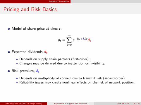
Model of share price at time t:
pt =∞∑s=0
e−(rs+δs )sds
Expected dividends ds
Depends on supply chain partners (first-order).Changes may be delayed due to inattention or invisibility.
Risk premium, δs
Depends on multiplicity of connections to transmit risk (second-order).Reliability issues may create nonlinear effects on the risk of network position.
John Birge and Jing Wu (Chicago Booth) Equilibrium in Supply Chain Networks June 20, 2016 4 / 29

Literature
Literature
1st-order effects
Industry level: Menzly & Ozbas (2007), Shahrur, Becker, & Rosenfeld (2010),Fruin, Osiol, & Wang (2012).
Firm level: Hendricks & Singhal (2003), Cohen & Frazzini (2008), Atalay,Hortacsu, & Syverson (2013, working).
2nd-order effects
Asset pricing: Sharpe (1964), Lintner (1965), Fama & French (1993).
Network risk: Acemoglu, Carvalho, Ozdaglar, & Tahbaz-Salehi (2012),Anupindi & Akella (1993), Cachon, Randall, & Schmidt (2007), Ahern (2012),Carvalho and Gabaix (2013), Kelly, Lustig, & Nieuwerburgh (2013, working),Herskovic (2014, working).
John Birge and Jing Wu (Chicago Booth) Equilibrium in Supply Chain Networks June 20, 2016 5 / 29

Data
Empirical Observations: Data
Scope is limited to U.S. public listed firms
Stock data: CRSP (monthly returns over July 2011 - June 2013)
Supply chain sales data (SPLC)
Compustat: SEC public filings (10% rule).
Bloomberg terminal (320k units): conference call transcripts, capital marketpresentations, firm press releases, product catalogs, firm websites.
Both are public information.
SEC’s Statement of Financial Accounting Standards No. 14 (SFAS 14)
“if 10% or more of the revenue of an enterprise is derived from sales to any singlecustomer, that fact and the amount of revenue from each such customer shall bedisclosed” in interim financial reports issued to shareholders
John Birge and Jing Wu (Chicago Booth) Equilibrium in Supply Chain Networks June 20, 2016 6 / 29
Data First-order Effects
Example Relationship
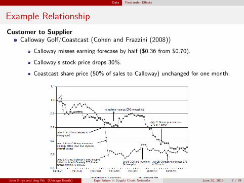
Customer to SupplierCalloway Golf/Coastcast (Cohen and Frazzini (2008))
Calloway misses earning forecase by half ($0.36 from $0.70).
Calloway’s stock price drops 30%.
Coastcast share price (50% of sales to Calloway) unchanged for one month.
John Birge and Jing Wu (Chicago Booth) Equilibrium in Supply Chain Networks June 20, 2016 7 / 29
Data First-order Effects
Example Relationship
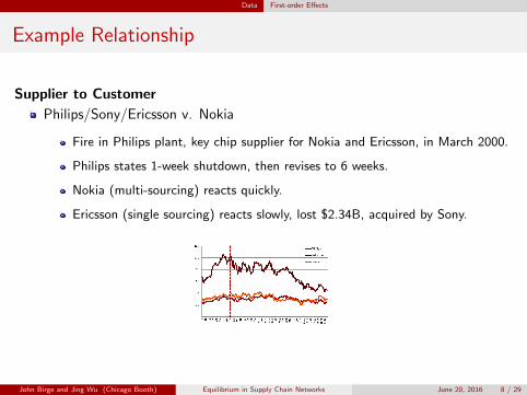
Supplier to Customer
Philips/Sony/Ericsson v. Nokia
Fire in Philips plant, key chip supplier for Nokia and Ericsson, in March 2000.
Philips states 1-week shutdown, then revises to 6 weeks.
Nokia (multi-sourcing) reacts quickly.
Ericsson (single sourcing) reacts slowly, lost $2.34B, acquired by Sony.
John Birge and Jing Wu (Chicago Booth) Equilibrium in Supply Chain Networks June 20, 2016 8 / 29

Data First-order Effects
First-order Effects
w inij denotes the supplier weight of j as a fraction of i ’s procurement.
woutij denotes the customer weight of j as a fraction of i ’s sales.
w inij =
salesjiProcurement i
=salesji∑Nk=1 saleski
,woutij =
salesijSales i
=salesij∑Nk=1 salesik
.
ri,t is the return of firm i in month t.
The following specification is tested:
ri,t = α + β1ri,t−1 + β2
∑j
w inij rj,t−1 + β3
∑j
woutij rj,t−1
+β4
∑j
w inij rj,t + β5
∑j
woutij rj,t + εi,t (1)
Hypothesis:
Suppliers’ and customers’ concurrent performance relates to the firm.Supplier momentum (one-month lag) may be related to firm performance(following Cohen and Frazzini (2008)).
John Birge and Jing Wu (Chicago Booth) Equilibrium in Supply Chain Networks June 20, 2016 9 / 29

Data First-order Effects
First-order Effects
Results
Table: Fama-Macbeth Regression of Concurrent Returns and Momentum.
α ri,t−1∑
j winij rj,t−1
∑j w
outij rj,t−1
∑j w
inij rj,t
∑j w
outij rj,t
Ave. Coef -0.001 -0.088*** 0.036** 0.024 0.399*** 0.755***(T-Stat) (-0.96) (-11.06) (2.17) (0.95) (20.90) (3.12)
Ave. Coef 0.009*** -0.090*** 0.057*** 0.004(T-Stat) (10.38) (-9.08) (2.96) (0.09)
Ave. Coef 0.009*** -0.047***(T-Stat) (10.53) (-6.96)
Ave. Coef 0.008*** 0.022**(T-Stat) (11.09) (1.83)
Ave. Coef 0.008*** -0.040(T-Stat) (10.92) (-0.66)
Ave. Coef 0.003*** 0.619***(T-Stat) (3.61) (37.25)
Ave. Coef -0.002** 0.992***(T-Stat) (-2.26) (4.54)
Ave. Coef 0.004*** 0.018* 0.625***(T-Stat) (4.51) (1.57) (36.44)
Ave. Coef -0.002* 0.001 1.001***(T-Stat) (-1.92) (0.0274) (4.51)
Ave. Coef -0.001* 0.393*** 0.744***(T-Stat) (-1.80) (22.48) (3.20)
*p-value<10%, **p-value<5%, ***p-value<1%
Controls: MKT, SMB, HML, MOM, cross-firm effect, industry effect.
John Birge and Jing Wu (Chicago Booth) Equilibrium in Supply Chain Networks June 20, 2016 10 / 29

Data Second-order Effects
Second-order Effects
Assumption
Acemoglu, Carvalho, Ozdaglar, & Tahbaz-Salehi (2012) (and the extension later)finds that microeconomic idiosyncratic shocks lead to aggregate flucturations,which meansA firm’s systematic risk is formed from the aggregation of idiosyncratic shocks.
Effects of connections may be nonlinear due to interactions - riskdiversification or aggregation?
Firm level shocks may be exogenously correlated due to geographicalproximity and sector proximity.
A manufacturer (e.g., Nokia) may have diversification incentives to add anindependent supplier to increase reliability (reduce systematic risk exposurewith greater centrality).A distributor (e.g., a beverage distributor) may have concentration incentivesto add similar suppliers (e.g., French wineries) to build on existing capabilities(increase systematic risk exposure with greater centrality).
John Birge and Jing Wu (Chicago Booth) Equilibrium in Supply Chain Networks June 20, 2016 11 / 29

Data Second-order Effects
Second-Order Results: Manufacturing
Table: Factor Sensitivities by Eigenvector Centrality for Manufacturing Firms.
N3 Factor Loadings
Portfolio α (%) Rmt − Rft SMB HML MOM Adj. R2(%)
1(High) 0.235 0.888*** 90.85(1.50) (15.47)0.114 0.894*** -0.347* 0.018 0.084 90.01(0.49) (12.23) (-2.07) (0.119) (1.025)
2 0.295* 0.773*** 88.74(1.78) (13.79)0.277 0.938*** -0.184 -0.453*** -0.061 93.77(1.34) (14.28) (-1.22) (-3.29) (-0.83)
3 0.328 1.060*** 92.78(1.33) (17.60)0.482* 0.953*** 0.363* -0.005 -0.008 93.04(1.86) (11.63) (1.93) (-0.03) (-0.09)
4 0.356 1.256*** 87.45(0.89) (12.97)0.571 1.087*** 0.446 0.130 -0.142 87.82(1.36) (8.22) (1.47) (0.47) (-0.96)
5(Low) 0.507 1.410*** 85.54(1.55) (11.96)0.934* 1.157*** 0.780** -0.257 -0.132 87.53(1.95) (7.63) (2.24) (-0.80) (-0.78)
High-Low -0.272* -0.522(-1.72) (-3.92)-0.820* -0.263 -1.127** 0.275 0.216(-1.96) (-1.28) (-2.40) (0.64) (0.94)
*p-value¡10%, **p-value¡5%, ***p-value¡1%
Controls: MKT, SMB, HML, MOM, cross-industry concentration.
John Birge and Jing Wu (Chicago Booth) Equilibrium in Supply Chain Networks June 20, 2016 12 / 29
Data Second-order Effects
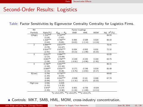
Second-Order Results: Logistics
Table: Factor Sensitivities by Eigenvector Centrality Centrality for Logistics Firms.
N4 Factor Loadings
Portfolio Alpha(%) Rmt − Rft SMB HML MOM Adj. R2(%)
1(High) 1.314*** 0.747*** 84.93(3.26) (7.62)
1.428*** 0.768*** 0.006 -0.589 0.024 86.43(3.44) (5.85) (0.02) (-2.14) (-0.16)
2 0.894*** 0.671*** 70.41(3.78) (11.67)
0.916*** 0.976*** 0.034 -0.502 0.031 72.32(2.41) (8.13) (0.13) (-1.99) (0.23)
3 0.812** 0.964*** 83.05(2.23) (10.89)
0.801** 0.758*** -0.140 -0.152 0.164 83.75(3.36) (10.03) (-0.81) (-0.96) (1.93)
4 0.708** 0.857*** 86.41(2.50) (12.40)
0.669** 0.916*** -0.171 -0.190 0.019 85.49(2.14) (9.26) (-0.75) (-0.92) (0.17)
5(Low) 0.759 0.776*** 69.60(1.44) (6.03)0.485 0.942*** -0.548 0.141 0.048 67.70(0.84) (5.17) (-1.31) (0.37) (0.23)
High-Low 0.556 -0.029(1.53) (-0.20)0.975* -0.175 0.553 -0.730 -0.024(1.93) (-0.90) (1.24) (-1.69) (-0.11)
*p-value¡10%, **p-value¡5%, ***p-value¡1%
Controls: MKT, SMB, HML, MOM, cross-industry concentration.
John Birge and Jing Wu (Chicago Booth) Equilibrium in Supply Chain Networks June 20, 2016 13 / 29

Data Second-order Effects
Second-Order Results: Mining, Utilities, and Construction
Table: Factor Sensitivities by Eigenvector Centrality for NAICS 2 Industries.
N2 Factor Loadings
Portfolio α (%) Rmt − Rft SMB HML MOM Adj. R2(%)
1(High) -1.153* 1.399*** 79.54(-1.74) (9.09)-1.179 1.458*** -0.091 -0.330 0.114 76.83(-1.52) (5.80) (-0.15) (-0.68) (0.45)
2 -0.897 1.512*** 79.42(-1.25) (9.06)-1.023 1.583*** -0.329 0.092 -0.103 76.28(-1.21) (5.76) (-0.48) (0.17) (-0.37)
3 -0.346 0.762*** 61.90(-0.62) (5.93)-0.680 0.935*** -0.458 0.262 0.155 59.96(-1.09) (4.63) (-0.92) (0.67) (0.76)
4 -0.374 1.129*** 72.88(-0.58) (7.58)-0.598 1.213*** -0.071 -0.376 0.261 71.72(-0.83) (5.20) (-0.12) (-0.84) (1.11)
5(Low) -0.479 1.339*** 78.22(-0.72) (8.74)-0.626 1.456*** -0.201 -0.215 0.221 75.94(-0.82) (5.90) (-0.33) (-0.45) (0.89)
High-Low -0.674* 0.060(-1.95) (1.25)-0.553 0.002 0.110 -0.115 -0.107(-1.51) (0.02) (0.51) (-0.68) (-1.20)
*p-value¡10%, **p-value¡5%, ***p-value¡1%
John Birge and Jing Wu (Chicago Booth) Equilibrium in Supply Chain Networks June 20, 2016 14 / 29

Data Second-order Effects
Centrality Implications to Different Industries
Both shock correlation and network topology matter for systematic risk.
Methodology:
Expected returns should be explained by all systematic risk factors.Split firms into quintiles based on centrality measures.If ∆α 6= 0 for two extreme quintile portfolios, supply chain network leads to”anomalies” in systematic risk.
Positions in the supply chain affects a firm’s exposure to the systematic riskbesides the network topology.
Upstream firms in manufacturing have diversification incentive to formsupplier connections to operationally hedge risk.Downstream firms in logistics have concentration incentive to form supplierconnections to leverage economy of scale thus aggregate risk.
John Birge and Jing Wu (Chicago Booth) Equilibrium in Supply Chain Networks June 20, 2016 15 / 29

Equilibrium Network Model
Simple Investment Model
Suppose an economy with 2 regions (A and B) and 3 potential future states belowwith equal probability (Prob (S = Si ) = 1
3 , ∀i ∈ 1, 2, 3):S1: both A and B function;S2: A cannot produce and B can;S3: B cannot produce and A can.Next, suppose 4 firms: 3 manufacturers and 1 distributor.Manufacturers: limited capacity and payoff of 1 as long as one input regionfunctions.Sources:
Firm 1 only from region AFirm 2 only from region BFirm 3 from both
Firm 4 is the distributor and connects to both A and B with a fixed cost of 1 in allstates.Payoffs:Π1 = 1, 0, 1, Π2 = 1, 1, 0, Π3 = 1, 1, 1, Π4 = 1, 0, 0.
John Birge and Jing Wu (Chicago Booth) Equilibrium in Supply Chain Networks June 20, 2016 16 / 29
Equilibrium Network Model
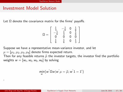
Investment Model Solution
Let Ω denote the covariance matrix for the firms’ payoffs.
Ω =
13 − 1
6 0 16
− 16
13 0 1
60 0 0 016
16 0 1
3
Suppose we have a representative mean-variance investor, and letµ = [µ1, µ2, µ3, µ4] denote firms expected return.Then for any feasible returns µ the investor targets, the investor find the portfolioweights w = [w1,w2,w3,w4] by solving
minww′Ωw |w
′µ = µ;w
′1 = 1′
,
John Birge and Jing Wu (Chicago Booth) Equilibrium in Supply Chain Networks June 20, 2016 17 / 29

Equilibrium Network Model
Simple Investment Results
The result of the equilibrium of investment is:µ1
µ2
µ3
µ4
=1
λ1
16w1 + 1
6w416w1 + 1
6w4
013w1 + 1
3w4
+λ2
λ1
Therefore,µ3 < µ1 = µ2 < µ4
i.e. the manufacturers have lower risk than the distributor, and the dual sourcingmanufacturer is less risky than the single sourcing manufacturer.Questions:
Does this result generalize to a broader classs of networks and what are otherempirical implications?Are the output representations consistent with an equilibrium model ofproduction?
John Birge and Jing Wu (Chicago Booth) Equilibrium in Supply Chain Networks June 20, 2016 18 / 29

Equilibrium Network Model
Equilibrium Network Model and Relationship to Literature
Previous literature focus on the sector level only.
Lucas (1977) argues that microeconomic shocks would average out at theaggregated level proportional to 1√
n.
Acemoglu et al. (2012) suggests Lucas (1977) only holds under symmetricnetwork structure, and microeconomic shocks may lead to aggregatedfluctuations in asymmetric networks.
The change in the density of firm level connections is not captured.
We build a supply chain network model using two-level nested productionfunction capturing both the firm-level and sector-level connections.
John Birge and Jing Wu (Chicago Booth) Equilibrium in Supply Chain Networks June 20, 2016 19 / 29

Equilibrium Network Model
Model Setup
An extension of Acemoglu et al. 2012
n industry sectors (S1, S2, ..., and Sn).
Firms in the same sector have the same Cobb-Douglas CRS productionfunction to produce perfectly substitutable products.
Supply chain relationships are established ex-ante.
xklij : output from firm l in sector j that inputs to firm k in sector i .
xi =∑
k∈Sixki : output from firm k in sector i .
xij =∑
k∈Si
∑l∈Sj
xklij : the production from sector j to sector i .
xi =∑
k∈Sixki : sector i ’s total production.
A unit labor allocating to to each firm (lki ) in each sector (li ), i.e.li =
∑k∈Si
lki and∑n
i=1 li = 1.
Consumption from by firm k in sector i is cki , and ci =∑
k∈Sicki .
Total consumption / GDP / labor wage is h.
John Birge and Jing Wu (Chicago Booth) Equilibrium in Supply Chain Networks June 20, 2016 20 / 29

Equilibrium Network Model
Competitive Equilibrium
A competitive equilibrium of economy
We define a competitive equilibrium of economy with n sectors consisting of prices(pi , i ∈ 1, ..., n), wage h, consumption bundle
(ci =
∑k∈Si
cki ,∀i , k ∈ Si), and
quantities(lki , x
ki , x
klij ,∀i , j , k, l
)such that
1 the representative consumer maximizes her utility;2 the firms in each sector maximizes their profits (0 in expectation);3 the labor and good markets clear at both levels, i.e. for any firm k in any
sector i , and for any sector i ,
xki = cki +n∑
j=1
∑l∈Sj
x lkji ,∑k∈Si
lki = li
xi = ci +n∑
j=1
xji ,n∑
i=1
li = 1
John Birge and Jing Wu (Chicago Booth) Equilibrium in Supply Chain Networks June 20, 2016 21 / 29
Equilibrium Network Model
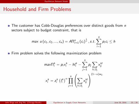
Household and Firm Problems
The customer has Cobb-Douglas preferences over distinct goods from nsectors subject to budget constraint, that is
max u (c1, c2, ..., cn) = AΠni=1 (ci )
1n , s.t.
n∑i=1
pici ≤ h
Firm problem solves the following maximization problem
maxΠki = pix
ki − hlki −
n∑j=1
pj∑l∈Sj
xklij
xki = zki(lki)α n∏
j=1
∑l∈Sj
xklij
(1−α)wij
John Birge and Jing Wu (Chicago Booth) Equilibrium in Supply Chain Networks June 20, 2016 22 / 29
Equilibrium Network Model
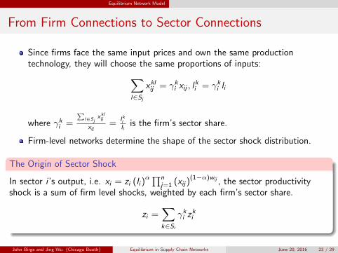
From Firm Connections to Sector Connections
Since firms face the same input prices and own the same productiontechnology, they will choose the same proportions of inputs:∑
l∈Sj
xklij = γki xij , lki = γki li
where γki =
∑l∈Sj
xklij
xij=
lkili
is the firm’s sector share.
Firm-level networks determine the shape of the sector shock distribution.
The Origin of Sector Shock
In sector i ’s output, i.e. xi = zi (li )α∏n
j=1 (xij)(1−α)wij , the sector productivity
shock is a sum of firm level shocks, weighted by each firm’s sector share.
zi =∑k∈Si
γki zki
John Birge and Jing Wu (Chicago Booth) Equilibrium in Supply Chain Networks June 20, 2016 23 / 29
Equilibrium Network Model
From Firm Connetions to Sector Connetions
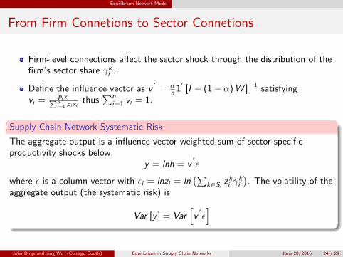
Firm-level connections affect the sector shock through the distribution of thefirm’s sector share γki .
Define the influence vector as v′
= αn 1′
[I − (1− α)W ]−1 satisfyingvi = pixi∑n
i=1 pixithus
∑ni=1 vi = 1.
Supply Chain Network Systematic Risk
The aggregate output is a influence vector weighted sum of sector-specificproductivity shocks below.
y = lnh = v′ε
where ε is a column vector with εi = lnzi = ln(∑
k∈Sizki γ
ki
). The volatility of the
aggregate output (the systematic risk) is
Var [y ] = Var[v′ε]
John Birge and Jing Wu (Chicago Booth) Equilibrium in Supply Chain Networks June 20, 2016 24 / 29
Equilibrium Network Model
Sparse v.s. Dense Supply Chain Networks
Sector B
Sector A
Sector B
Sector A
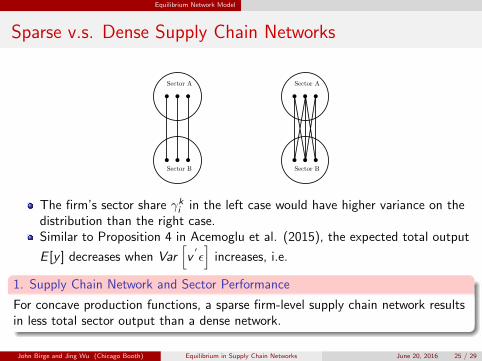
The firm’s sector share γki in the left case would have higher variance on thedistribution than the right case.Similar to Proposition 4 in Acemoglu et al. (2015), the expected total output
E [y ] decreases when Var[v′ε]
increases, i.e.
1. Supply Chain Network and Sector Performance
For concave production functions, a sparse firm-level supply chain network resultsin less total sector output than a dense network.
John Birge and Jing Wu (Chicago Booth) Equilibrium in Supply Chain Networks June 20, 2016 25 / 29
Equilibrium Network Model
Simulation
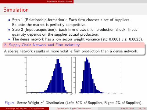
Step 1 (Relationship-formation): Each firm chooses a set of suppliers.Ex-ante the market is perfectly competitive.Step 2 (Input-acquisition): Each firm draws i.i.d. production shock. Inputquantity depends on the supplier actual production.The dense network has a low sector weight variance (std 0.0001 v.s. 0.0023).
2. Supply Chain Network and Firm Volatility
A sparse network results in more volatile firm production than a dense network.
8.8 9 9.2 9.4 9.6 9.8 10 10.2 10.4 10.6
x 10−3
0
200
400
600
800
1000
1200
0 0.005 0.01 0.015 0.02 0.025 0.03 0.0350
200
400
600
800
1000
1200
1400
Figure: Sector Weight γki Distribution (Left: 80% of Suppliers, Right: 2% of Suppliers).
John Birge and Jing Wu (Chicago Booth) Equilibrium in Supply Chain Networks June 20, 2016 26 / 29

Equilibrium Network Model
Simulation (cont.)
Both cases exhibit sizable and systematic deviations from the normaldistribution (2%: heavy left tail, 80%: heavy right tail).Only the sector weight with modest connection density is normal distributed.
Sufficient Statistics for Firm Production Variation
With firm-level supply chain connection variation, there is no guarantee that thefirm-level production is normally distributed.
−4 −3 −2 −1 0 1 2 3 49
9.2
9.4
9.6
9.8
10
10.2
10.4
10.6
10.8x 10⁻³
Standard Normal Quantiles
Qua
ntile
s of
Inpu
t Sam
ple
QQ Plot of Sample Data versus Standard Normal
−4 −3 −2 −1 0 1 2 3 40
0.005
0.01
0.015
0.02
0.025
Standard Normal Quantiles
Qua
ntile
s of
Inpu
t Sam
ple
QQ Plot of Sample Data versus Standard Normal
Figure: Q-Q Plot of the Sector Weight γki Distribution (Left: 80% of Suppliers, Right:
2% of Suppliers).John Birge and Jing Wu (Chicago Booth) Equilibrium in Supply Chain Networks June 20, 2016 27 / 29
Equilibrium Network Model
More Concentrated Economic Activities during Crisis.
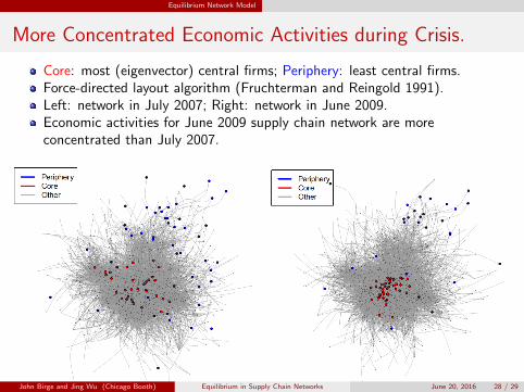
Core: most (eigenvector) central firms; Periphery: least central firms.Force-directed layout algorithm (Fruchterman and Reingold 1991).Left: network in July 2007; Right: network in June 2009.Economic activities for June 2009 supply chain network are moreconcentrated than July 2007.
Figure: Network in July 2007
Figure: Network in June 2009
John Birge and Jing Wu (Chicago Booth) Equilibrium in Supply Chain Networks June 20, 2016 28 / 29

Conclusions & Future Directions
Conclusions and Future Directions
Evidence of concurrent supplier and customer effects plus suppliermomentum effects on returns.
Investors’ limited attention to supplier firms relative to customer firms.Gradual diffusion of supply chain information downstream as opposed toupstream.
Evidence of decreasing returns to centrality in manufacturing and increasingreturns to centrality in logistics.
Supply chain structure is an ex-ante determined and ex-post identifiable sourcefor systematic risk.Upper-stream utility, mining, and construction firms behave similarly asmanufacturing.
Equilibrium model of firms connecting across sectors
Natural hedging decisions from manufacturersLower volatility effect for manufacturers implies conditions for increasingconections to cause lower risk for upstream and higher risk for downstream
Future DirectionsAdditional empirical tests (including default propagation)Incorporate of investment into the model formulation
John Birge and Jing Wu (Chicago Booth) Equilibrium in Supply Chain Networks June 20, 2016 29 / 29