A Fuzzy Logic Algorithm for Dense Image Point Matching

Christian B. U. PerwassInstitut fur Informatik

CAU Kiel,24105 Kiel, Germany

christian@perwass.com

Gerald SommerInstitut fur Informatik

CAU Kiel,24105 Kiel, Germany

gs@ks.informatik.uni-kiel.de

March 13, 2001

Abstract

We present a conceptually simple algorithm for dense imagepoint matching between two colour images. The algorithmis based on the assumption that the topology only changesslightly between the two images. Following this assumptionwe use an iterative fuzzy inference process to find the likeli-est image point matches. Advantages of this algorithm arethat it is fundamentally parallel, it does not need any exactgeometric information about the cameras and it can alsogive image point matches within homogeneous areas of thetwo images.

1 Introduction

Image point matching is important for many aspects ofComputer Vision. Most notably for stereo vision and op-tical flow [1]. There are a number of strategies to reducethe complexity of the problem in the case of stereo vision.One is to simplify the task by extracting features in the twoimages, which are then matched [2, 3]. An obvious draw-back of this approach is, that only certain areas of the imagesare matched. Of course, depending on the application, thismay be sufficient. However, feature based 3D reconstruc-tion from a stereo image pair only gives us a sparse modelof the 3D world.

There are quite a number of algorithms which producedense disparity maps, given the geometry of the camera sys-tem [4, 5, 6, 7]. Most of these algorithm make their decisionslocally without taking into account global constraints on theimage point matches. Marr and Poggio [8, 9] were one of thefirst to apply global constraints to dense disparity map algo-rithms. Their assumptions about stereo were uniqueness andcontinuity of a disparity map. We apply similar constraintsdirectly to the images. An interesting paper in this context is[10], where a scale-based connectedness on images is usedfor image segmentation.

In [11] Barnard and Thompson present an algorithmwhich also assumes a continuous disparity map. They use

this constraint to find the disparity of feature points in twoimages, exploiting the fact that nearby feature points shouldhave similar disparity values. The probability of the cor-rect disparity values is then estimated through an iterativerelaxation labeling technique. The basic ideas in [11] arequite similar to our fundamental matching strategy. How-ever, their algorithm only applies to feature points and theactual implementation of the constraints is quite different toours.

Another approach to dense matching is to assume thatthere is an affine transformation between the two images[12]. Finding the appropriate affine transformation is thena least squares problem. A drawback of this approach is thatthe parameter search space might be quite big. Furthermore,the approximation of what is really a projective transforma-tion by an affine transformation, may fail for close rangeobjects.

In this paper we present an algorithm which attempts tomatch two colour images pixel by pixel. To achieve this wemake somequalitativeassumptions about the geometry ofthe camera system that took the images and the 3D objectswe look at. We donot need to know the exact epipolar ge-ometry of the camera setup, though.

2 Theory

The general task of matching two images taken from quitedifferent view points of the same 3D object, is quite hard.Here we try to simplify this task by making certain assump-tions about the camera setup and the 3D objects we look at.

1. The two cameras are separated more or less horizon-tally by a small distance.

2. The vertical axes of the two cameras are approximatelyaligned and the optical axes point to the same area inthe 3D scene.

3. There are no depth discontinuities in the 3D scene.

1

First of all note that these assumptions are only of aqual-itative nature. That is, we do not need to know the exactgeometry of the camera setup. Assumption 3 is quite strict,especially since there are typically quite a number of depthdiscontinuities in 3D scenes. The effect of this assumptionwill be discussed later on.

Assumptions 1 and 2 basically model the geometry ofthe human visual system. They ensure that the changes inthe two generated images are not too big, i.e. in the order ofa few pixels. Taking the three assumptions together gives usyet another bit of information. Let us denote the two givenimages byA andB, respectively. A pixel at position(x, y)in imageA is denoted byAx,y and similarly for imageBby Bx,y. Let (Ai,j , Br,s) be a pixel match between imagesA andB. Then it follows from the three assumptions thatpixel Ai+1,j should have a matchnearBr+1,s in imageB,and similarly for the other pixels adjacent toAi,j . That is,we basically assume that the topology of the two images issimilar.

In order to use this information we have to be able toevaluate the similarity between two pixels. When using grayimages this is simply the difference between the gray valuesof the pixels. However, gray images contain much less in-formation than colour images, which is why we chose touse the latter. Evaluating the similarity of two colour pixelsis not as straight forward as for gray pixels, though. Themethod we used is described later. For now let us assumethat we have a functionψ(Ai,j , Br,s) which gives the simi-larity between pixelsAi,j andBr,s. ψ returns a value in therange[0, 1] ⊂ R, whereby1 denotes equality and0 inequal-ity. Calculatingψ for each pixel in imageA with all pixelsin imageB gives a set of similarity distributions. We de-fine Ψi,j

r,s ≡ ψ(Ai,j , Br,s), which can be regarded as a fourdimensional, discrete fuzzy set. For each(i, j) the matrixΨi,j•,• is thus a 2 dimensional, discrete fuzzy set. Looking at

the similarity distributions in this way, we can start thinkingabout applying fuzzy logic operators to these sets.

Before we start describing the algorithm, we will givea very short introduction to fuzzy sets and fuzzy operators.Fuzzy sets can be used to describe inexact or ”fuzzy” infor-mation. With standard sets we can either say that an object isan element of this set or not. That is, for any subsetA ⊂ Xof some setX there exists a functionfA : X → {0, 1},which says for any elementx ∈ X whetherx ∈ A or not. IffA(x) = 1 thenx ∈ A and if fA(x) = 0 thenx 6∈ A. Theidea behind fuzzy sets is to define adegree of membershipby a value between0 and1. In order to model a fuzzy setAonX, a membership functionµA : X → [0, 1] is introducedwhich returns the degree of membership of anyx ∈ X toA.In our algorithm we can interpret eachΨi,j as a fuzzy set,where the degree of membership of a pixelBr,s to this set isgiven byΨi,j

r,s, the discrete membership function.Fuzzy setsA,B can also be combinedA ∪ B and inter-

sectedA ∩B. This is done through their membership func-

tionsµA, µB , via two functionss, t : [0, 1]× [0, 1] → [0, 1],the so calleds-norm andt-norm. That is,µA∪B(x) :=s(µA(x), µB(x)) andµA∩B := t(µA(x), µB(x)). The ac-tual form ofs andt depends on the application. The func-tionss, t may for example be defined asmax,min, respec-tively. In this way,s represents the logical OR operator andt the logical AND operator. An appropriate choice ofs andt is in fact quite important for our algorithm.

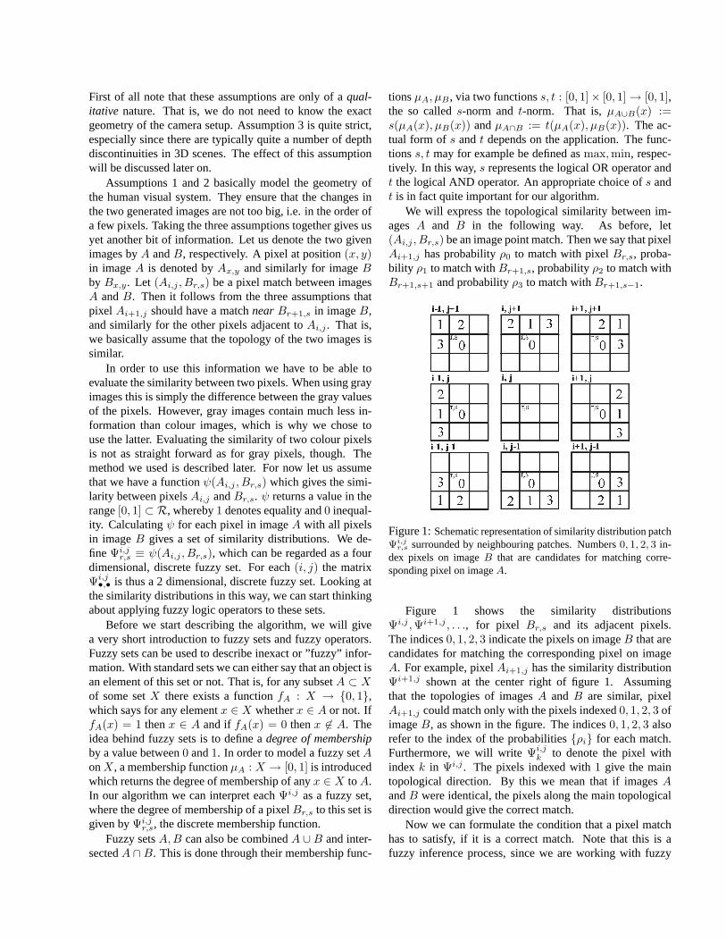
We will express the topological similarity between im-agesA and B in the following way. As before, let(Ai,j , Br,s) be an image point match. Then we say that pixelAi+1,j has probabilityρ0 to match with pixelBr,s, proba-bility ρ1 to match withBr+1,s, probabilityρ2 to match withBr+1,s+1 and probabilityρ3 to match withBr+1,s−1.

Figure 1:Schematic representation of similarity distribution patchΨi,j

r,s surrounded by neighbouring patches. Numbers0, 1, 2, 3 in-dex pixels on imageB that are candidates for matching corre-sponding pixel on imageA.

Figure 1 shows the similarity distributionsΨi,j ,Ψi+1,j , . . ., for pixel Br,s and its adjacent pixels.The indices0, 1, 2, 3 indicate the pixels on imageB that arecandidates for matching the corresponding pixel on imageA. For example, pixelAi+1,j has the similarity distributionΨi+1,j shown at the center right of figure 1. Assumingthat the topologies of imagesA andB are similar, pixelAi+1,j could match only with the pixels indexed0, 1, 2, 3 ofimageB, as shown in the figure. The indices0, 1, 2, 3 alsorefer to the index of the probabilities{ρi} for each match.Furthermore, we will writeΨi,j

k to denote the pixel withindex k in Ψi,j . The pixels indexed with1 give the maintopological direction. By this we mean that if imagesAandB were identical, the pixels along the main topologicaldirection would give the correct match.

Now we can formulate the condition that a pixel matchhas to satisfy, if it is a correct match. Note that this is afuzzy inference process, since we are working with fuzzy

sets. The AND (∧) and OR (∨) operators we will use inthe following therefore refer to fuzzy logic operators. Inprinciple they may be implemented with anyt-norm ands-norm, respectively.

We evaluate the confidence that a point pair(Ai,j , Br,s)is indeed an image point match, using the following expres-sion. [ ∧

(u,v)

(∨k

(ρkΨi+u,j+vk )

)]∧ Ψi,j

r,s, (1)

wherek ∈ {0, 1, 2, 3} and(u, v) ∈ S, with

S :={

(1, 0), (1, 1), (0, 1), (−1, 1),

(−1, 0), (−1,−1), (0,−1), (1,−1)}.

The inner OR operation of equation (1) goes over all in-dexed pixels for the particularΨi+u,j+v similarity distribu-tion. The outer AND operation counts over all similaritydistributions surrounding the central distribution. The setSsimply defines the appropriate offset vectors.

In words equation (1) says that the point pair(Ai,j , Br,s)is an image point match if the pixels themselves are sim-ilar AND pixel Ai+1,j is similar toBr,s OR Br+1,s ORBr+1,s+1 ORBr+1,s−1, AND pixel Ai+1,j+1 is similar toBr,s OR etc.

The confidence value returned by equation (1) lies in therange[0, 1]. We could use this value directly or as the inputto some decision functionφ. To stay as general as possible,we will use the latter. Applying equation (1) for each pair ofimage points produces a new set of confidence values.

Φi,jr,s := φ

([ ∧(u,v)

(∨k

(ρkΨi+u,j+vk )

)]∧ Ψi,j

r,s

). (2)

Φi,jr,s gives a confidence measure that pixelAi,j corresponds

to pixelBr,s. Qualitatively, this is the same asΨi,jr,s, since

higher similarity between pixel colours also means higherlikelihood that the pixels correspond to each other. Hence,we could use equation (2) recursively by replacingΨ withΦ.

EvaluatingΦ enhances the confidence measure for thosepixel matches that have a high confidence themselves andwhose neighbouring pixel matches also have high confi-dences. The confidence measure of matches where this isnot the case is reduced. The effect of iterating equation (2)once is that also the match confidence information from twopixels distance to every pixel is taken into account. For ex-ample, after the first evaluation ofΦ, the confidence measureof Φi+1,j

r,s is based onΨi+2,jr,s and other elements ofΨ. After

iterating equation (2) once the confidence measure ofΦi,jr,s

is based onΦi+1,jr,s , which in turn is based onΨi+2,j

r,s . If wekeep on iterating, larger and larger structures have an influ-ence on the matching of every pixel. Therefore, it should

also be possible to match over homogeneous areas in im-ages, as long these areas are bounded by borders and weiterate long enough so that the whole structure is taken intoaccount. Note that the transformation between two imagesis found here by allowing the topology to change slightly ona pixel scale.

3 Implementation

Although the algorithm presented in the last section is quitesimple in principle, there are a number aspects we need togive some more thought to, in order to implement it. Weneed to give the exact form of the functionsψ andφ andchoose appropriatet- ands-norms for the AND and OR op-erations in equation (2). Furthermore,Ψ andΦ can becomequite large and evaluating them is computationally expen-sive. However, note that iterating equation (2) is emulatinga feedback process. In principle this algorithm could be im-plemented as a large neural network which performs one it-eration in a single step. Nevertheless, we implemented thealgorithm on a standard computer, which imposed a numberof constraints.

First of all we demanded in the last section thatΨ andΦ are evaluated for each pixel in imageA over all pixel inimageB. This is clearly not feasible for large images. Inorder to reduce the computational load we define a ”sourcepatch” in imageA and a ”target patch size” for imageB.Then Φ and Ψ are evaluated for each pixel in the sourcepatch of imageA over a target patch in imageB. However,now we have the problem of where to place the target patchin imageB. This means we need to have an initial imagepoint match(Ai,j , Br,s). Then the target patch for pixelAi,j

is centered aboutBr,s. In fact,(Ai,j , Br,s) does not need tobe an exact match. We only have to demand that the correctmatch forAi,j lies within the target patch centered onBr,s.Still, we might run into problems if the correct match forAi,j lies right at the border of the target patch. Note that by”correct match” we mean the best match available. Due tonoise on the images and the transformations present, therewill typically not be anexactmatch.

Finding the first approximate match is quite simple in thecase of optical flow. We just choose the centers of imagesA andB, since it is the same camera that took the two im-ages within a short time. We could also select a number ofpoints from which the algorithm is started simultaneously.Of course, there may be situations when this strategy fails.

The situation is more difficult for a stereo camera pair.Here we would first need a method to adjust the camerasuntil their optical axes cross near a point in the 3D scene.Then we could again use the image centers of imagesA andB as the approximate first match. Note that the concept ofattention will play an important role in such a method. Ifwe had a sufficiently fast implementation of the algorithm

presented here, we could use it to adjust the geometry of thestereo camera system, until a proper match is found, usingthe image centers as an approximate initial match.

For now we will assume that an approximate initial im-age point match is given by(Ai,j , Br,s), say. Then we canfind Ψi,j for the target patch centered onBr,s. However,if we center the target patch for pixelAi+1,j aboutBr,s, aswell, its correct match may not lie within this target patch.Therefore, we center the target patch for someAi+u,j+v onBr+u,j+v, i.e. on the pixel along the main topological direc-tion. This means, of course, that the correct match for someAi+u,j+v may lie outside the corresponding target patch, ifthe topology has deviated sufficiently from the main topo-logical direction. In effect, this constrains the size of thesource patch.

In the following we will denote thenth iteration ofΦi,jr,s

by nΦi,jr,s, whereby we define0Φi,j

r,s ≡ Ψi,jr,s. We can there-

fore write equation (2) as

(n+1)Φi,jr,s = φ

([ ∧(u,v)

(∨k

(ρknΦi+u,j+v

k ))]

∧ nΦi,jr,s

),

(3)with n ≥ 0. At each iterationnΦi,j

r,s is evaluated for eachpixel in the source patch over all pixel in the correspond-ing target patch. Performing the inner OR operation is thensimply a component wise OR operation on the matricesnΦi+u,j+v

k , with an appropriate offset. For example, the ma-trix nΦi+1,j

1 has no offset, since it was evaluated along themain topological direction and the target patches are cen-tered on the pixel along this direction. The matrixnΦi+1,j

0

has to be offset by one pixel to the right before ORing it withnΦi+1,j

1 (see figure 1). In this way the inner OR operation ofequation (3) is performed for all pixel in the target patch inone step. Because the target patches are of finite dimensions,offsetting a matrix introduces an additional row or column.We set this extra row or column to zero before performingthe OR operation. This means that the pixels right at theborder of a target patch will not take into account as muchinformation as the inner pixels. Note that before ORing thematrices we also multiply them component wise with theprobabilities{ρk}.

We found that the inner OR operation is representedwell by the max function. For the AND operation overthe elements ofS we investigated a number of fuzzy op-erators. Two different operators produced good results: theλ-operator and themean operation. Theλ-operator is a mix-ture between the algebraic product and the algebraic sum. Itis defined as

fλ(a, b) := λ [ab] + (1−λ) [a+ b− ab] , λ ∈ [0, 1]. (4)

If λ = 0, fλ(a, b) gives the algebraic sum ofa andb, whichcompares to an OR operation. Ifλ = 1, fλ(a, b) gives thealgebraic product ofa andb, which corresponds to an AND

operation. That is, theλ-operator can be something in be-tween AND and OR. We found that forλ = 1 the itera-tion converged quickly to a good match, because spuriousmatches are eliminated quickly. However, sometimes cor-rect matches are also eliminated prematurely, which makesthe iteration unstable. This is because the algebraic productis a ”strict” AND operator: it is enough if one of the ele-ments is zero in order to make the whole result zero. Thus,if the confidence for a single pixel match goes to zero itwill propagate through the whole image and make all confi-dences zero. This is clearly not what we intended. Smallervalues forλ reduce this effect but also increase the numberof iterations needed to obtain good matches.

A better way to express the AND operation is throughthe mean operation. That is, AND becomes an oper-ation ”between” OR and AND. Here we take the meancomponent-wise over all matrices. In this way, a single, oreven a few, zero components do not make the result zero.Using themean operation stabilizes the iteration process,although more iterations are needed to obtain a good match.However, this should also be somewhat desired, because wewant larger structures to have an influence on the matchingprocess. Nevertheless, for the outer AND operation in equa-tion (3) we use the algebraic product. This gives a goodcompromise between speed and stability.

Another important choice is the form of the functionφ.So far we have not found a completely satisfactoryφ, al-though the following implementation works quite well. LetnΦi,j

r,s be defined bynΦi,jr,s = φ(nΦi,j

r,s). Theφ we use scales

each matrixnΦi,j•,• separately, such that the largest compo-

nent of the matrix becomes1. This scaling is necessary be-cause we are using a single byte for each confidence valuedue to memory constraints. Furthermore, the confidencevalues tend to become smaller and smaller with each itera-tion. With this renormalization applied throughφ, we makesure that each matrixnΦi,j

•,• has at least one confident match.This is also the disadvantage of using thisφ, because in real3D scenes we do have depth discontinuities and thus occlu-sion, which in turn means that not every pixel in imageAneeds to have a match in imageB. If occlusion occurs, thealgorithm will give the next best match for the pixel. Futurework will investigate how to incorporate occlusion into thisalgorithm in a better way.

There is one part of the algorithm left which we have notdiscussed, yet. This is the form of the functionψ. Recallthatψ should give the similarity of two pixel. This may bebased on any kind of information, not just their colours. Werestrictedψ to give the similarity of two pixels only basedon their colours, though. Of course, this poses the questionwhich colour space to use and how to obtain a similaritymeasure [13]. Since this is not essential to our algorithm,we will use the simplest way to represent the colour of apixel, namely as a 3D-vector in an RGB-colour space. Thedifference between two colours represented by colour vec-

torsc1 andc2 may then be calculated as||c1 − c2||. How-ever, this means that black and white are more different fromeach other than are black and red, say. Phenomenologically,white should be regarded as as different from black, as red isfrom black, though. For our purposes it would be desirablethat all pairs of colours black, white, red, green and blue, areregarded as being equally dissimilar. This can be achievedin the following way.

Let ∆ = c1 − c2, and denote the components of∆ by(δr, δg, δb) with δr, δg, δb ∈ [0, 1]. Then we find the similar-ity of coloursc1 andc2 as follows.

ψ(c1, c2) = 1− ||∆||||∆/max(δr, δg, δb)||

, (5)

if c1 6= c2. Forc1 = c2 we defineψ(c1, c2) = 1.To summarize, equation (3) takes the following form in

our implementation.

(n+1)Φi,jr,s =

[18

∑(u,v)

supk

(ρk

nΦi+u,j+vk

)]∗ nΦi,j

r,s, (6)

andnΦi,j

r,s =nΦi,j

r,s

supr,s

(nΦi,j

r,s

) (7)

4 Experiments

Figure 2:Initial image of mug.

We present here three experiments with real images toshow some aspects of the algorithm. Figures 2 and 3 showtwo images of a coffee mug taken from slightly different po-sitions. These images of the mug were taken with a digitalcamera with a resolution of1024 × 768 pixels. This reso-lution was reduced to200× 150 pixels in a post-processingstep. For the following test we used the center of the flowerat the top left as the starting point for the algorithm. Thesource patch was41 × 41 pixels and the target patch7 × 7pixels. Note that the source and target patches do not needto be square. However, the target patch should have odddimensions.

Figure 3:Image of mug from a slightly different perspective.

Figure 4:Reconstructed image of translation test.

Figure 5:Flow field of translation test.

The {ρk} from equation (3) were set to the followingvalues: ρ1 = 1 andρ0 = ρ2 = ρ3 = 0.9. That is, themain topological direction was slightly preferred. The re-sult images are shown after20 iterations which took about 3

minutes and 20 seconds. The computer used was a PentiumII with 233 MHz running Windows Me.

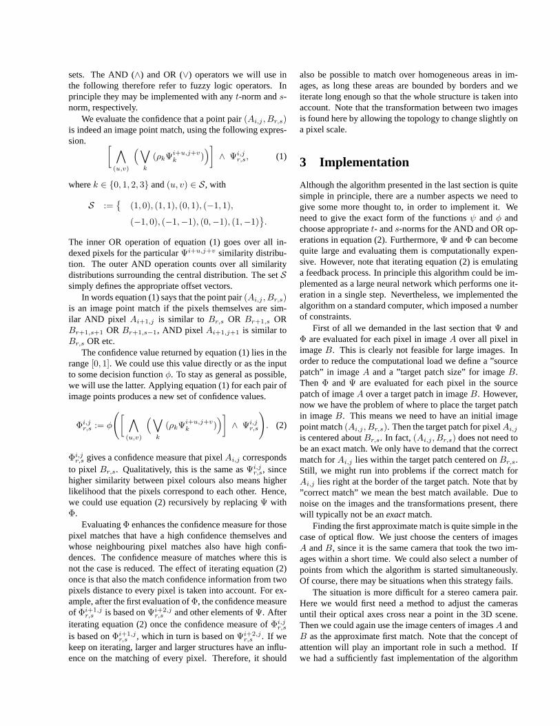
Figure 6:Image of mug rotated clockwise by 10 degrees.

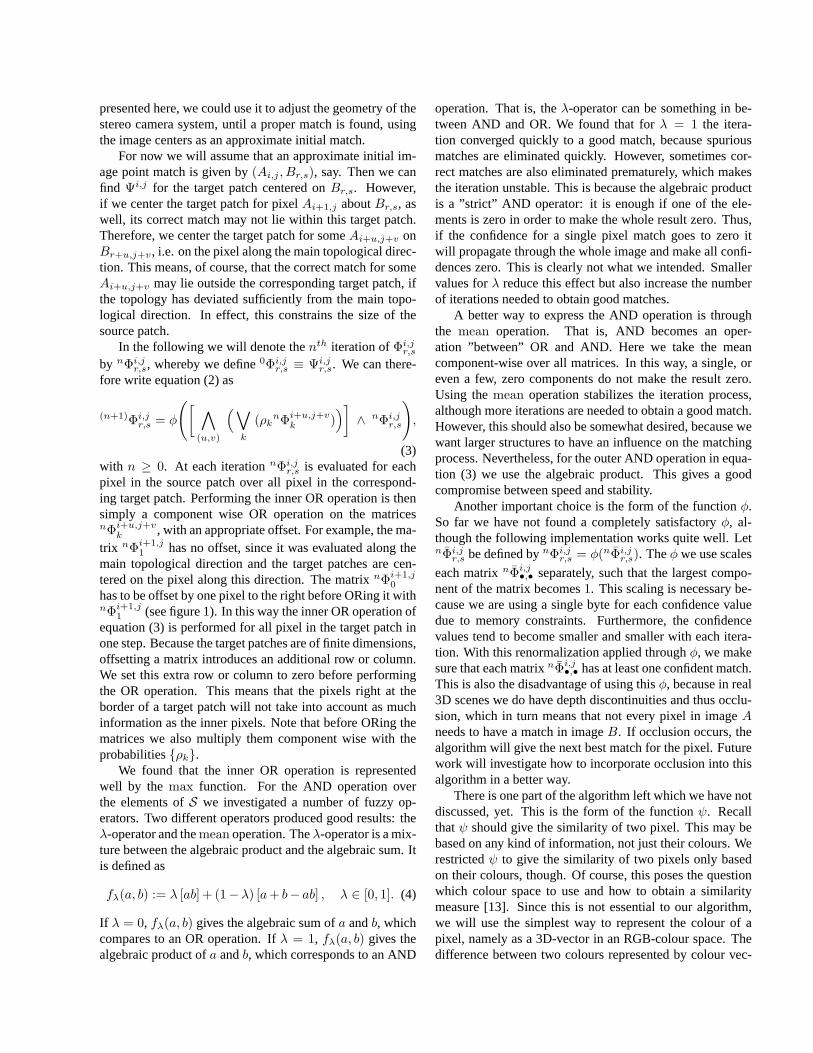
Figure 7:Reconstructed image of rotation test after 7 iterations.

The implementation of the algorithm was not optimizedfor speed but for adaptability. In any event, real time ca-pability is most likely to be achieved by a hardware imple-mentation of the network structure that lies at the root of thealgorithm.

First we present a simple test which shows the behaviourof the algorithm with ideal data. In this experiment we usedthe image in figure 2 as both, source and target image. How-ever, the initial image point match used was off by two pix-els to the right and two pixels down. The reconstructed im-age after 20 iterations is presented in figure 4 and the corre-sponding flow field in figure 5. Since the reconstruction andflow field are drawn relative to the target pixel of the initialimage point match, we should expect the reconstruction tobe translated two pixels to the left and two pixels up, with acorresponding flow field. This is exactly what we find. Notethat the correct flow is also found for homogeneous areas inthe image.

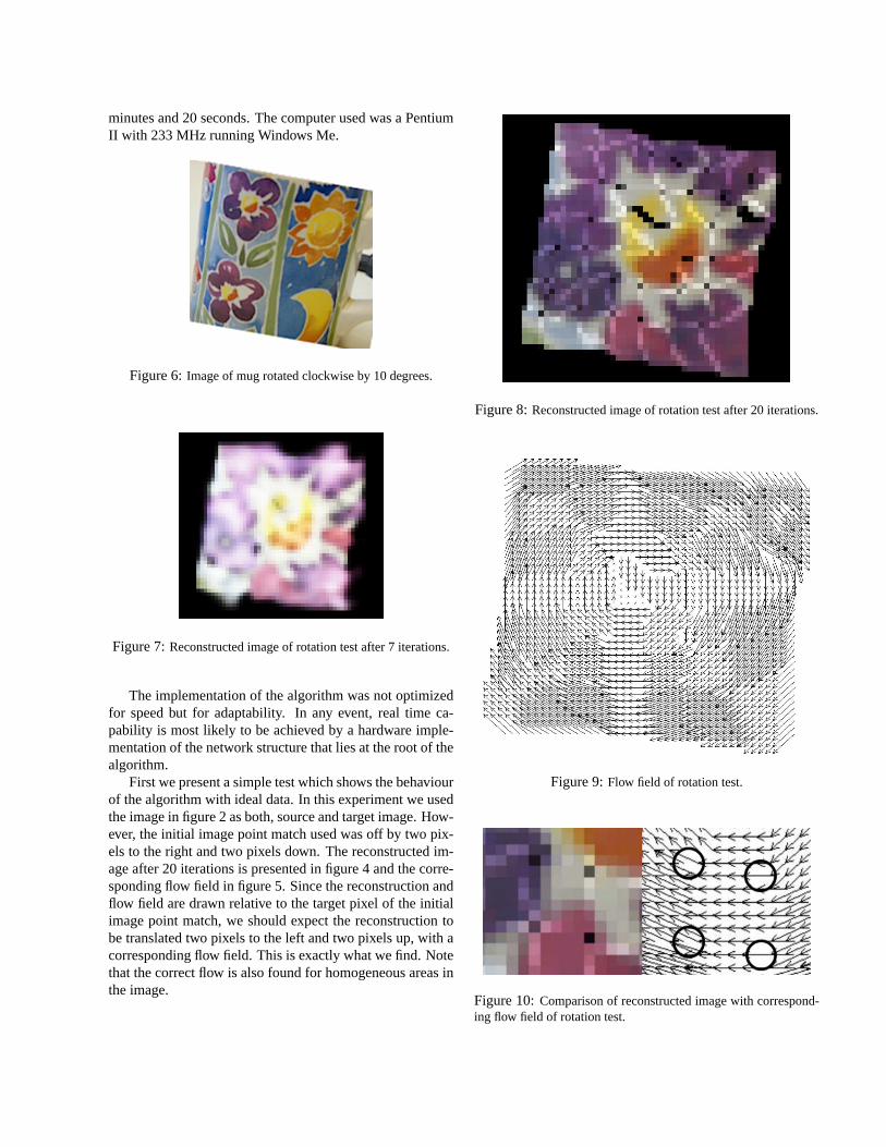
Figure 8:Reconstructed image of rotation test after 20 iterations.

Figure 9:Flow field of rotation test.

Figure 10:Comparison of reconstructed image with correspond-ing flow field of rotation test.

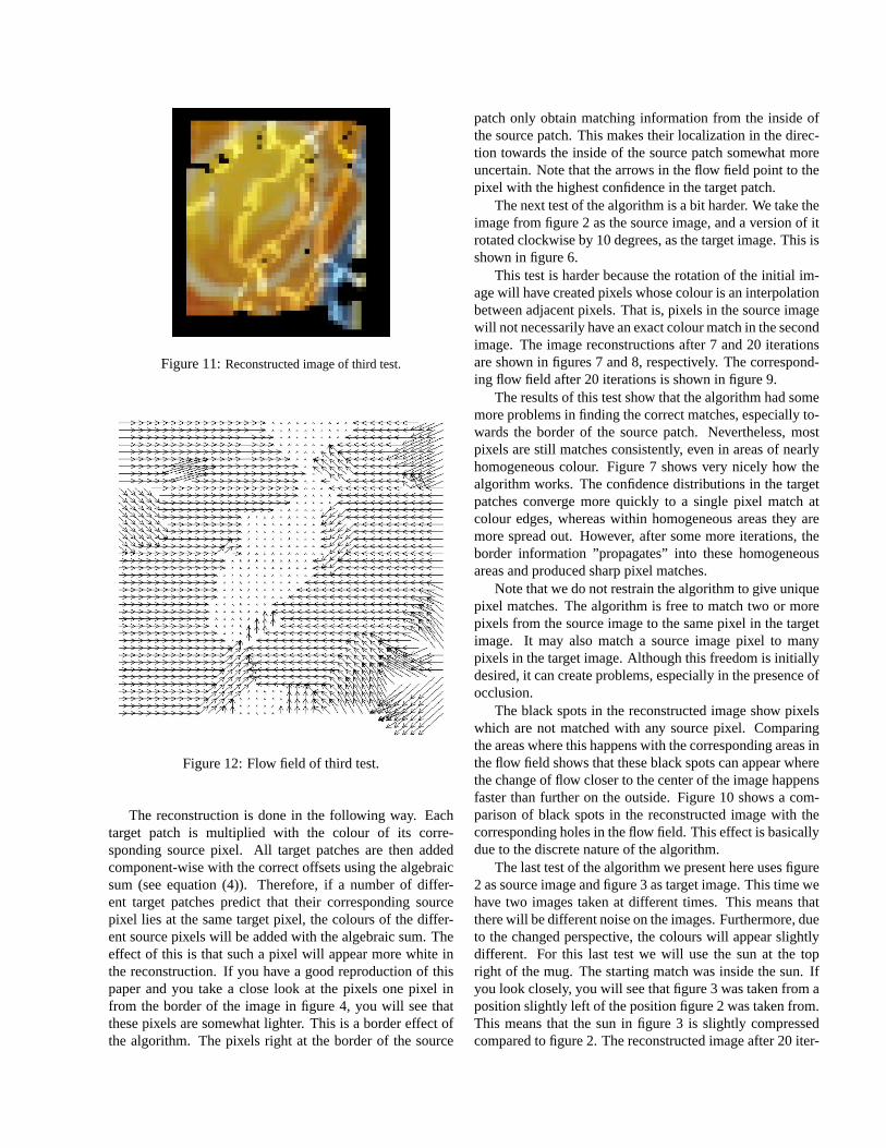
Figure 11:Reconstructed image of third test.

Figure 12: Flow field of third test.

The reconstruction is done in the following way. Eachtarget patch is multiplied with the colour of its corre-sponding source pixel. All target patches are then addedcomponent-wise with the correct offsets using the algebraicsum (see equation (4)). Therefore, if a number of differ-ent target patches predict that their corresponding sourcepixel lies at the same target pixel, the colours of the differ-ent source pixels will be added with the algebraic sum. Theeffect of this is that such a pixel will appear more white inthe reconstruction. If you have a good reproduction of thispaper and you take a close look at the pixels one pixel infrom the border of the image in figure 4, you will see thatthese pixels are somewhat lighter. This is a border effect ofthe algorithm. The pixels right at the border of the source

patch only obtain matching information from the inside ofthe source patch. This makes their localization in the direc-tion towards the inside of the source patch somewhat moreuncertain. Note that the arrows in the flow field point to thepixel with the highest confidence in the target patch.

The next test of the algorithm is a bit harder. We take theimage from figure 2 as the source image, and a version of itrotated clockwise by 10 degrees, as the target image. This isshown in figure 6.

This test is harder because the rotation of the initial im-age will have created pixels whose colour is an interpolationbetween adjacent pixels. That is, pixels in the source imagewill not necessarily have an exact colour match in the secondimage. The image reconstructions after 7 and 20 iterationsare shown in figures 7 and 8, respectively. The correspond-ing flow field after 20 iterations is shown in figure 9.

The results of this test show that the algorithm had somemore problems in finding the correct matches, especially to-wards the border of the source patch. Nevertheless, mostpixels are still matches consistently, even in areas of nearlyhomogeneous colour. Figure 7 shows very nicely how thealgorithm works. The confidence distributions in the targetpatches converge more quickly to a single pixel match atcolour edges, whereas within homogeneous areas they aremore spread out. However, after some more iterations, theborder information ”propagates” into these homogeneousareas and produced sharp pixel matches.

Note that we do not restrain the algorithm to give uniquepixel matches. The algorithm is free to match two or morepixels from the source image to the same pixel in the targetimage. It may also match a source image pixel to manypixels in the target image. Although this freedom is initiallydesired, it can create problems, especially in the presence ofocclusion.

The black spots in the reconstructed image show pixelswhich are not matched with any source pixel. Comparingthe areas where this happens with the corresponding areas inthe flow field shows that these black spots can appear wherethe change of flow closer to the center of the image happensfaster than further on the outside. Figure 10 shows a com-parison of black spots in the reconstructed image with thecorresponding holes in the flow field. This effect is basicallydue to the discrete nature of the algorithm.

The last test of the algorithm we present here uses figure2 as source image and figure 3 as target image. This time wehave two images taken at different times. This means thatthere will be different noise on the images. Furthermore, dueto the changed perspective, the colours will appear slightlydifferent. For this last test we will use the sun at the topright of the mug. The starting match was inside the sun. Ifyou look closely, you will see that figure 3 was taken from aposition slightly left of the position figure 2 was taken from.This means that the sun in figure 3 is slightly compressedcompared to figure 2. The reconstructed image after 20 iter-

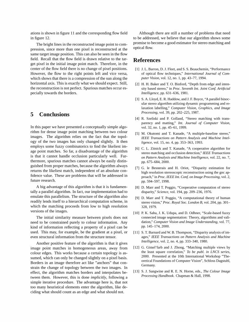
ations is shown in figure 11 and the corresponding flow fieldin figure 12.

The bright lines in the reconstructed image point to com-pression, since more than one pixel is reconstructed at thesame target image position. This can also be seen in the flowfield. Recall that the flow field is drawn relative to the tar-get pixel in the initial image point match. Therefore, in thecenter of the flow field there is no change of pixel positions.However, the flow to the right points left and vice versa,which shows that there is a compression of the sun along thehorizontal axis. This is exactly what we should expect. Still,the reconstruction is not perfect. Spurious matches occur es-pecially towards the borders.

5 Conclusions

In this paper we have presented a conceptually simple algo-rithm for dense image point matching between two colourimages. The algorithm relies on the fact that the topol-ogy of the two images has only changed slightly. It thenemploys some fuzzy combinatorics to find the likeliest im-age point matches. So far, a disadvantage of the algorithmis that it cannot handle occlusion particularly well. Fur-thermore, spurious matches cannot always be easily distin-guished from proper matches, because the algorithm alwaysreturns the likeliest match, independent of an absolute con-fidence value. These are problems that will be addressed infuture research.

A big advantage of this algorithm is that it is fundamen-tally a parallel algorithm. In fact, our implementation had toemulate this parallelism. The structure of the algorithm alsoreadily lends itself to a hierarchical computation scheme, inwhich the matching proceeds from low to high resolutionversions of the images.

The initial similarity measure between pixels does notneed to be constrained purely to colour information. Anykind of information reflecting a property of a pixel can beused. This may, for example, be the gradient at a pixel, oreven structural information from the structure tensor.

Another positive feature of the algorithm is that it givesimage point matches in homogeneous areas, away fromcolour edges. This works because a certain topology is as-sumed, which can only be changed slightly on a pixel basis.Borders in an image therefore act like ”anchors” that con-strain the change of topology between the two images. Ineffect, the algorithm matches borders and interpolates be-tween them. However, this is doneimplicitly, following asimple iterative procedure. The advantage here is, that nottoo many heuristical elements enter the algorithm, like de-ciding what should count as an edge and what should not.

Although there are still a number of problems that needto be addressed, we believe that our algorithm shows somepromise to become a good estimator for stereo matching andoptical flow.

References[1] J. L. Barron, D. J. Fleet, and S. S. Beauchemin, “Performance

of optical flow techniques,”International Journal of Com-puter Vision, vol. 12, no. 1, pp. 43–77, 1994.

[2] H. H. Baker and T. O. Binford, “Depth from edge and inten-sity based stereo,” inProc. Seventh Int. Joint Conf. ArtificialIntelligence, pp. 631–636, 1981.

[3] S. A. Lloyd, E. R. Haddow, and J. F. Boyce, “A parallel binoc-ular stereo algortihm utilizing dynamic programming and re-laxation labelling,”Computer Vision, Graphics, and ImageProcessing, vol. 39, pp. 202–225, 1987.

[4] R. Szeliski and P. Golland, “Stereo matching with trans-parency and matting,”Int. Journal of Computer Vision,vol. 32, no. 1, pp. 45–61, 1999.

[5] M. Okutomi and T. Kanade, “A multiple-baseline stereo,”IEEE Transactions on Pattern Analysis and Machine Intel-ligence, vol. 15, no. 4, pp. 353–363, 1993.

[6] C. L. Zitnick and T. Kanade, “A cooperative algorithm forstereo matching and occlusion detection,”IEEE Transactionson Pattern Analysis and Machine Intelligence, vol. 22, no. 7,pp. 675–684, 2000.

[7] G. le Besnerais and H. Oriot, “Disparity estimation forhigh resolution stereoscopic reconstruction using the gnc ap-proach,” inProc. IEEE Int. Conf. on Image Processing, vol. 2,pp. 594–597, 1998.

[8] D. Marr and T. Poggio, “Cooperative computation of stereodisparity,”Science, vol. 194, pp. 209–236, 1976.

[9] D. Marr and T. Poggio, “A computational theory of humanstereo vision,”Proc. Royal Soc. London B, vol. 204, pp. 301–328, 1979.

[10] P. K. Saha, J. K. Udupa, and D. Odhner, “Scale-based fuzzyconnected image segmentation: Theory, algorithms and vali-dation,”Computer Vision and Image Understanding, vol. 77,pp. 145–174, 2000.

[11] S. T. Barnard and W. B. Thompson, “Disparity analysis of im-ages,”IEEE Transactions on Pattern Analysis and MachineIntelligence, vol. 2, no. 4, pp. 333–340, 1980.

[12] G. Gimel’farb and J. Zhong, “Matching multiple views bythe least square correlation,”To be publ. in LNCS series,2000. Presented at the 10th International Workshop ”The-oretical Foundations of Computer Vision”, Schloss Dagstuhl,Germany.

[13] S. J. Sangwine and R. E. N. Horne, eds.,The Colour ImageProcessing Handbook. Chapman & Hall, 1998.