A Fully Unsupervised Non-intrusive LoadMonitoring Framework

Ruoxi Jia, Yang Gao, Costas J. Spanos

Department of Electrical Engineering and Computer ScienceUniversity of California, Berkeley

Berkeley, CA 94720, USAEmail: {ruoxijia,yg,spanos}@berkeley.edu

Abstract—Monitoring an individual electrical load’s energyusage is of great significance in energy-efficient buildings as itunderlies the sophisticated load control and energy optimizationstrategies. Non-intrusive load monitoring (NILM) provides aneconomical tool to access per-load power consumption withoutdeploying fine-grained, large-scale smart meters. However, exist-ing NILM approaches require training data to be collected bysub-metering individual appliances as well as the prior knowledgeabout the number of appliances attached to the meter, which areexpensive or unlikely to obtain in practice. In this paper, wepropose a fully unsupervised NILM framework based on Non-parametric Factorial Hidden Markov Models, in which per-loadpower consumptions are disaggregated from the composite signalwith minimum prerequisite. We develop an efficient inferencealgorithm to detect the number of appliances from data anddisaggregate the power signal simultaneously. We also proposea criterion, Generalized State Prediction Accuracy, to properlyevaluate the overall performance for methods targeting at bothappliance number detection and load disaggregation. We eval-uate our framework by comparing against other multi-taskingschemes, and the results show that our framework comparesfavorably to prior work in both disaggregation accuracy andcomputational overhead.

I. INTRODUCTION

Buildings contribute to more than 40% of the total en-ergy consumption in US [1]. The provision of per-load en-ergy data in realtime can support ”smart” buildings withimproved energy-efficiency. For instance, an automated loadscheduling policy can be designed to reduce a building’speak power demand by deferring one or more backgroundloads with knowledge of energy usage and the duration ofeach background load. Building occupants can also learn theenergy consumption of appliances and are empowered to takenecessary actions to save energy. However, one major andcontinuing impediment of energy efficiency improvement isthat deployment and maintenance of fine-grained power metersin a large scale are costly and cumbersome.

Rather than relying on expensive instrumentation, an alter-native approach is non-intrusive load monitoring (NILM), alsoknown as power disaggregation, which analyzes the aggregatedpower data from a single smart meter and aims to break it downto individual appliances’ power usage. Generally speaking,the NILM process involves the following steps of Detection,Disaggregation and Designation (3D for short):

• Appliance Detection

• Load Disaggregation

• Multi-state Designation

Appliance detection aims to find how many appliances(loads) are attached to the power meter of concern. Mostresearch work has considered the number of loads as a priorknowledge and then analyzes the composite power signal usingfixed-size models [2]. However, it is an eminently practicalconcern that the number of appliances in buildings can hardlybe consistent over time. Ignorance of this fact would lead toimproper choice of the models and thereby degrade disag-gregation performance. Simply choosing a model sufficientlycomplex in order to accommodate an arbitrarily chosen largenumber of hypothetical loads will induce large computationaloverhead.

Load disaggregation consists of determining the ON/OFFstate and power consumption of individual appliances given thecomposite signal. A common category of load disaggregationmethods assumes that sub-metered ground truth data is avail-able for training prior to performing disaggregation [3]–[6].This assumption dramatically increases the investment requiredto set up such a system, since in reality deploying sub-metersmay be inconvenient or time-consuming. The second categoryincludes model-driven approaches that relax requirements fortraining data [7], [8]. Parson et al. [9] proposed to tunethe generic appliance models to specific appliance instancesusing signatures extracted from the aggregate load. Tang etal. [10] formulated load disaggregation as an optimizationproblem and tried to minimize the variation of switchingevents based on the knowledge of appliance power modelsand the sparsity of the switching events. The third categoryof load disaggregation approaches obviates the need of theprior knowledge of appliances using unsupervised learningmethods [11]–[13], which however often requires the numberof appliances to be known.

Most of aforementioned work has made the assumptionabout a binary nature of appliance states. However, in prac-tice appliances might have multiple states beyond OFF state,such as active mode, stand-by mode, etc. An appliance withmultiple states may be detected as to two or more two-stateappliances. The multi-state designation step is to merge statescorresponding to the same appliance.

In this paper, we develop an fully unsupervised NILMframework without the need of sub-metered data or the prior

knowledge about the number of appliances, and integrate 3Dprocess using the Bayesian network. The main contributionsare summarized as follows:

• We establish a simultaneous appliance detection, loaddisaggregation and multi-state designation framework usingnonparametric Bayesian models, which, to our knowledge, hasnot been used to solve the power disaggregation problem.

• We develop an efficient inference algorithm pertaining tothe nonparametric Bayesian model, which takes advantage ofslice sampling to adaptively truncate the size of model basedon the number of appliances.

•We propose a metric that can standardize the performanceevaluation procedure for power disaggregation frameworkwithout the prior knowledge about the number of appliances.We also evaluate our framework using the real-world datacollected in public dataset, REDD [14]. The result showsthe superiority of our framework to other appliance numberdetection and load disaggregation schemes based on traditionalmodel selection.

II. PROBLEM FORMULATION

In this section, we formalize the problem of power disag-gregation. Suppose we are given an aggregated power signaly(t) from K appliances with t from 1 to T . Here, we do notassume any prior knowledge of the number of appliances, i.e.K is unknown. Let Z be a T × K matrix and (t, k)-entryzt,k indicates the state for appliance k at time t. The goal isto determine state matrix Z from the aggregated power signaly. We assume that each appliance has two states (ON/OFF)and its power consumption follows the Gaussian distributionwhen the appliance is ON. As can be seen from Fig. 1,the assumption is valid for most appliances, while for someappliances, e.g. laptop, the multimodality of the distribution isevident. This is because appliances might have multiple stateswith distinctive power consumptions when they are ON, suchas active-mode and standby-mode. Even though they mighthave multiple states, they can be considered as comprisingtwo or more binary-state appliances. We will first define Z asa binary matrix in which 0/1 stand for OFF/ON respectivelyand further introduce a state designation algorithm to mergeON states corresponding to the same appliance.

III. PROPOSED FRAMEWORK

From the description of energy disaggregation problemin the preceding section, it is evident that the number ofappliances determines the dimension of state space to be esti-mated and thereby is directly related to the model complexityand computational overhead. Previous work determines theappropriate model by first learning a set of model candidatesand select one using comparison metrics [15]. Rather thancomparing models that vary in complexity, Bayesian nonpara-metric models are featured in fitting a single model that canadapt its complexity to the data by imposing a prior on modelparameters. Inspired by this, in this section we will present ourframework, a Nonparametric Factorial Hidden Markov Model(NFHMM), which can automate appliance detection processto load disaggregation. We will start by providing a briefbackground on Factorial Hidden Markov Model and IndianBuffet Process, based upon which we will describe our blind

(a) (b)

(c) (d)

(e) (f)

Fig. 1: Normalized histogram of (a) oven (b) microwave (c)kitchen outlet (d) lighting (e) laptop. The power distributionof some appliances can be well approximated by Gaussiandistribution, while other appliances appear to be multi-modal.

(a) (b)

Fig. 2: (a) HMM (b) FHMM.

source disaggregation framework, NFHMM, for binary stateappliance. Finally, we extend the binary state case to multiplestates by introducing our multi-state designation algorithm.

A. Factorial Hidden Markov Model (FHMM)

FHMM is originally proposed in [16] as a distributed staterepresentation of HMM (Fig. 2). Due to its distributed nature,FHMM is useful to model multiple loosely-coupled processesand has been considered as a method for power disaggregation[2]. In the FHMM, the state for each of K appliances evolvesvia a HMM independently and the states for all appliances attime t jointly determine the observation at time t.

B. Indian Buffet Process (IBP)

IBP has been studied by machine learning community asa prior in probabilistic models that represent a potentiallyinfinite array of f

eatures. IBP is defined as a limit of the distributionover binary matrices with a finite number of rows andunbounded number of columns and is suitable to derive theprobability of state matrix Z in our setting. In the originalIBP, each entry of Z is drawn from a Bernoulli distributionparameterized by a Beta prior. Since the columns K areunbounded, the probability of Z is generally not well defined.Note that each appliance is exchangeable in the sense thatwe only care about the partitioning of the composite signalrather than the ordering of each appliance, therefore we cancompute the probability of the equivalence classes of Z whichcorrespond to the identical form via permutation of columns.In this way, an analytic formula for infinite-dimensional statematrix Z can be found and the derivation is elaborated in[17].

C. Nonparametric Factorial Hidden Markov Model (NFHMM)

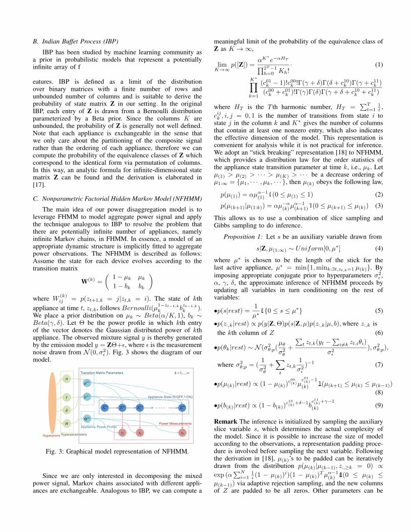
The main idea of our power disaggregation model is toleverage FHMM to model aggregate power signal and applythe technique analogous to IBP to resolve the problem thatthere are potentially infinite number of appliances, namelyinfinite Markov chains, in FHMM. In essence, a model of anappropriate dynamic structure is implicitly fitted to aggregatepower observations. The NFHMM is described as follows:Assume the state for each device evolves according to thetransition matrix

W(k) =

(1− µk µk1− bk bk

)where W

(k)ij = p(zt+1,k = j|zt,k = i). The state of kth

appliance at time t, zt,k, follows Bernoulli(µ1−zt−1,k

k bzt−1,k

k ).We place a prior distribution on µk ∼ Beta(α/K, 1), bk ∼Beta(γ, δ). Let Θ be the power profile in which kth entryof the vector denotes the Gaussian distributed power of kthappliance. The observed mixture signal y is thereby generatedby the emission model y = ZΘ+ε, where ε is the measurementnoise drawn from N (0, σ2

ε ). Fig. 3 shows the diagram of ourmodel.

α

γ

δ

µ (k )

b(k )

HΘ(k )

Z0(k ) Z1

(k ) Z2(k ) ZT

(k )

y1 y2 yT

Appliance State (0:OFF,1:ON)

Power Measurements

Transition Matrix Parameters

Appliance Power Profile

Hyperparameters Hyperpriors

k = 1,...,∞

Fig. 3: Graphical model representation of NFHMM.

Since we are only interested in decomposing the mixedpower signal, Markov chains associated with different appli-ances are exchangeable. Analogous to IBP, we can compute a

meaningful limit of the probability of the equivalence class ofZ as K →∞,

limK→∞

p([Z]) =αK

∗e−αHT∏2T−1

h=0 Kh!· (1)

K∗∏k=1

(c01k − 1)!c00k !Γ(γ + δ)Γ(δ + c10k )Γ(γ + c11k )

(c00k + c01k )!Γ(γ)Γ(δ)Γ(γ + δ + c10k + c11k )

where HT is the T th harmonic number, HT =∑Tt=1

1t ,

cijk , i, j = 0, 1 is the number of transitions from state i tostate j in the column k and K∗ gives the number of columnsthat contain at least one nonzero entry, which also indicatesthe effective dimension of the model. This representation isconvenient for analysis while it is not practical for inference.We adopt an “stick breaking” representation [18] to NFHMM,which provides a distribution law for the order statistics ofthe appliance state transition parameter at time k, i.e., µk. Letµ(1) > µ(2) > · · · > µ(K) > · · · be a decrease ordering ofµ1:∞ = {µ1, · · · , µk, · · · }, then µ(k) obeys the following law,

p(µ(1)) = αµα−1(1) 1(0 ≤ µ(1) ≤ 1) (2)

p(µ(k+1)|µ(1:k)) = αµ−α(k)µα−1(k+1)1(0 ≤ µ(k+1) ≤ µ(k)) (3)

This allows us to use a combination of slice sampling andGibbs sampling to do inference.

Proposition 1: Let s be an auxiliary variable drawn from

s|Z, µ(1:∞) ∼ Uniform[0, µ∗] (4)

where µ∗ is chosen to be the length of the stick for thelast active appliance, µ∗ = min{1,mink:∃t,zt,k=1 µ(k)}. Byimposing appropriate conjugate prior to hyperparameters σ2

ε ,α, γ, δ, the approximate inference of NFHMM proceeds byupdating all variables in turn conditioning on the rest ofvariables:

•p(s|rest) =1

µ∗1{0 ≤ s ≤ µ∗} (5)

•p(z:,k|rest) ∝ p(y|Z,Θ)p(s|Z, µ)p(z:,k|µ, b),where z:,k isthe kth column of Z (6)

•p(θk|rest) ∼ N (σ2θ;p(

µθσ2θ

+

∑t zt,k(yt −

∑i 6=k zt,iθi)

σ2ε

), σ2θ;p),

where σ2θ;p = (

1

σ2θ

+∑t

zt,k1

σ2ε

)−1 (7)

•p(µ(k)|rest) ∝ (1− µ(k))c00(k)µ

c01(k)−1(k) 1(µ(k+1) ≤ µ(k) ≤ µ(k−1))

(8)

•p(b(k)|rest) ∝ (1− b(k))c10(k)+δ−1b

c11(k)+γ−1(k) (9)

Remark The inference is initialized by sampling the auxiliaryslice variable s, which determines the actual complexity ofthe model. Since it is possible to increase the size of modelaccording to the observations, a representation padding proce-dure is involved before sampling the next variable. Followingthe derivation in [18], µ(k)’s to be padded can be iterativelydrawn from the distribution p(µ(k)|µ(k−1), z:,≥k = 0) ∝exp (α

∑Ni=1

1i (1 − µ(k))

i)(1 − µ(k))Tµα−1(k) 1(0 ≤ µ(k) ≤

µ(k−1)) via adaptive rejection sampling, and the new columnsof Z are padded to be all zeros. Other parameters can be

expanded via sampling the corresponding prior distribution.Sampling of the second quantity is done by a combinationof block Gibbs sampler and a standard Forward FilteringBackward Sampling procedure. The posterior distributions ofthe remaining variables θk, µ(k) and b(k) are proven to besimple Gaussian or Beta distribution. Moreover, by imposingappropriate conjugate prior to hyperparameters, the posteriordistributions of hyperparameters are all of simple analyticforms. Algorithm 1 summarizes the inference algorithm ofNFHMM.

Algorithm 1 NFHMM Inference Algorithm

Input: y: Aggregate power signalInitialization :Z, µ, b, θIterNum← Maximum iteration numberIterative Sampling :

1: while IterNum > 0 do2: Sample slice variable s (Eqn. (5))3: Expand representation of Z, µ, b, θ (Remark)4: Sample Z with a blocked Gibbs sampler and run FFBS

on each column of Z (Eqn. (6))5: Sample θ, µ, b (Eqn. (7), (8), (9))6: Sample hyperparameters α, γ, δ, µθ, σ2

θ , σ2ε (Remark)

IterNum← IterNum− 17: end while

Output: Z, θ

D. Resolving Multiple States of an Appliance

In the discussion above, we have assumed that each ap-pliance has binary states, ON/OFF, while in practice mul-tiple states with different power consumption levels mightbe associated with different usage conditions of one singleappliance. Fig. 4 shows real power traces of a laptop and arefrigerator, which is a superposition of spikes and a relativeconstant base power level. The baseline power presents thepower consumption level in normal cases while spikes canbe an indicator of overuse, charging process, etc. The keyobservation that supports our multi-state designation algorithmis that the ”abnormal” mode of appliances always appears tobe temporary and concurs with the baseline power. We cancombine the ”abnormal” mode with normal one by noticingthe time slot of transient abnormalities is a subset of normalusage time. Let’s formalize this in the following proposition:

Proposition 2: Let Sk to be the set of time slots withinwhich the appliance k is ON, i.e.

Sk = {[ts, te] : ts ≤ t ≤ te, zkt = 1, zkts = 0, zkte = 0}(10)

Denote the cardinality of the set Sk to be |Sk|. Assume thecomposite power signal is aggregated from some small numberof appliances, then for some appliance i and j, if the criterion

|Si ∩ Sj ||Si|

> 1− τ (11)

is satisfied, then we claim the two columns of Z, zi: and zj:, arethe states corresponding to the identical appliance. τ is somesmall positive integer indicating the fuzziness of matching.

(a) (b)

Fig. 4: Real power traces of (a) the laptop and (b) therefrigerator. Single appliance can generate multiple states withdifferent power levels.

IV. EXPERIMENTAL EVALUATION

Our proposed framework has been evaluated using Ref-erence Energy Disaggregation Dataset (REDD) (http://redd.csail.mit.edu/) described in [14]. This dataset was chosenas it is benchmark dataset specifically collected for testingNILM algorithms. The REDD comprises six houses, for whichboth aggregate and circuit-level power consumption data weremonitored. [14] and [11] provide two benchmarked disag-gregation results using supervised and unsupervised methodrespectively based on FHMM. Our framework differs fromprevious methods since we target not only at disaggregating thecomposite power signal without labeled data but also deducingthe number of appliances from observed signals, thereforea direct performance comparison is not possible. However,we will benchmark our method against the combination ofunsupervised disaggregation and traditional statistical modelselection procedure. To be specific, we come up with severalFHMMs with fixed sizes and experiment these models with theAkaike Information Criterion (AIC) and Bayesian InformationCriterion (BIC), which are commonly adopted in model selec-tion [19].

A. Evaluation Metrics

State prediction accuracy is a commonly used evaluationmetric if the number of appliances is provided as priorknowledge. However, nonparametric disaggregation methodsaim at integrating the appliance detection and load disag-gregation process, and thereby other metrics are required inorder to evaluate the capability of predicting correct numberof appliances. We propose a Generalized State PredictionAccuracy (GSPA) that standardizes the evaluation process fornonparametric disaggregation methods.

This metric is inspired by the maximum weight bipartitematching problem in graph theory. Nonparametric disaggre-gation methods are likely to produce different estimates ofthe appliance number. Therefore, an appropriate evaluationmetric would take both the number of appliances and theON/OFF state of each appliance into account when comparingthe ground truth with some algorithmic prediction. Calculationof GSPA involves two steps: Firstly, find the correspondencebetween predicted appliances and groundtruth. Then we cal-culate a numeric score based on the matching quality andappliance relative importance which is indicated by the ONtime duration.

For the first step, in order to obtain the correspondencebetween ground truth appliances and predicted appliances,we calculate a pairwise accuracy score between the predictedappliance i and ground truth appliance j, defined as

wij =|Ψi ∩Ψj ||Ψi ∪Ψj |

(12)

where Ψi is the time slots when appliance i is estimated to beON and Ψj is the period of time when appliance j in groundtruth is ON. If i and j correspond to the identical applianceand the state estimation is perfect, then wij = 1. In thisway, the correspondence finding problem is converted to themaximum weight matching problem if considering estimatedappliance set and ground truth appliance set as a bipartite(Fig. 5). We use Hungarian algorithm [20] to calculate thebest matching for weight matrix wij . This will be our bestguess for the correspondence between predicted appliancesand the ground truth appliances, and the accuracy of thebest matching correspondence is considered to be the stateestimation accuracy. Since we would like to produce a metricthat also takes into consideration the correctness of appliancenumber prediction and relative importance of appliances, wewill define GSPA score in the following way: Assume that wehave matched predicted appliance ik to ground truth appliancejk for k = 1 · · ·min(Kpre,Kgt), where Kpre and Kgt are thepredicted and actual number of appliances respectively. TheGSPA score is defined to be the appliance-importance weightedsum of accuracy associated with a penalty of predicting thewrong number of appliances.

GSPA =

∑min(Kpre,Kgt)k=1 πjkwik,jk∑min(Kpre,Kgt)

k=1 πjk + penalty(13)

where πjk is the ON time ratio of the ground truth appliancejk. The penalty term is the sum of the ON time ratio of theappliances which do not have correspondence. We refer tothese appliances as ghost appliances, which may be createddue to random noise or abnormalities of appliance operations.The GSPA will penalize prediction error in the frequently-used appliances more than in the seldom-used ones, and willalso penalize missing real appliances and predicting ghostappliances.

In addition to GSPA, we also use running time as a metricto measure the computational overhead.

B. Framework Validation

We first demonstrate the validity of our framework bydecomposing the aggregated signal from three appliances:oven, refrigerator and light in a randomly picked time interval.The mixed and original power consumption for each applianceare shown in Fig. 6 (a) and 6 (c), respectively. It can be seenthat different electrical loads exhibit distinctive power levels.For these three appliances, the power signals tend to fluctuatearound a fixed value during ON state, in which case our Gaus-sian assumption for the appliance power is held and therebywe expect a good separation for these devices. Fig. 6 (d) showsthe state estimation of each appliance given by our algorithmand Fig. 6 (b) gives corresponding ground truth. Here, weuse heatmaps to demonstrate appliance’s state at a certaintimestamp, where rows are appliances, columns are white if

(a)

w11

w21

w31

w12 w13 w14

w22 w23 w24

w32 w33 w34

Gro

und

Trut

h

Appliance Estimation

Maximum Weight Matching

(b)

Fig. 5: GSPA metric: (a) Compute accuracy for all possiblepairs between ground truth and appliance estimation (Theground truth contains 3 appliances while 4 appliances areestimated by nonparamteric disaggregation methods in theexample); (b) Calculate the maximum weight matching.

(a) (b)

(c) (d)

Fig. 6: NFHMM can detect the state of each appliance withoutprior knowledge of the number of appliances: (a) Aggregatedpower signal we try to decompose; (b) Ground truth of the stateof each appliance: rows are appliances, columns are white ifthe appliance is ON and black otherwise; (c) Ground truth ofpower traces of appliances, summing up which we obtain themixed signal in (a); (d) Estimate of the appliance state.

the appliance is ON and black otherwise. Visual inspectionof two heatmaps shows that our algorithm achieves almost aperfect detection of appliances’ states with the accuracy of98.5%, and it can also give a correct estimation of the numberof appliances simultaneously. Fig. 7 illustrates the convergenceperformance by showing how disaggregation accuracy variesas iteration numbers increase. As can be seen, our algorithmexhibits different convergence rate for different runs and therealways exists a steep increase of accuracy instead of growingsteadily. It is worth noting that the accuracy keeps above 75%even with only one step iteration.

Since our framework disaggregates power signal using onlylow frequency real power feature and assumes binary statesfor appliances, the single appliance with multiple power usage

Iteration Number0 10 20 30 40 50 60 70 80 90 100

Accu

racy

0.7

0.75

0.8

0.85

0.9

0.95

1Convergence Rate

round 1round 2round 3

Fig. 7: Convergence of NFHMM: The accuracy grows asiteration steps increase. Even with only one iteration, theaccuracy is above 75 %

Time

Pow

er (W

) (a) Ground Truth

(b) State Estimation by NFHMM

(c) After State Designation

App

. No.

A

pp. N

o.

Fig. 8: Demonstration of the state designation algorithm: (a)The ground truth of the power consumption signals of a laptopin which multiple power usage modes are evident; (b) The stateestimation result given by NFHMM inference where an extraappliance is produced for the high power usage mode; (c) Thefinal state estimation result after applying the state designationalgorithm where the extra appliance is eliminated.

modes is possible to be recognized as multiple appliances.Fig. 8 shows a snapshot of the ambiguity. As aforementioned,the laptop can have distinctive power consumption levelsdepending on the different usage conditions. Our algorithmtends to add appliances to explain the higher power usage,shown in Fig. 8(b). Nevertheless, following up the cue thatthe ”abnormalities” always appear to be transient spikes super-posed upon the baseline power, we apply our state designationalgorithm to the preliminary result given by NFHMM and the“ghost” device that represents the active mode of the laptopcan be merged (Fig. 8(c)).

C. Comparative Study

We scale up our experiments by aggregating all regularly-used appliances in one house and make a comparison of results

TABLE I: Performance comparison between NFHMM andFHMMs selected by AIC and BIC.

GSPA score Time (s) Appliance Number

NFHMM 0.2510 12 7

FHMM+AIC 0.2350 304 4

FHMM+BIC 0.1223 304 13

produced by our framework against FHMM models selectedby AIC [21] and BIC [22].

The composite signal is aggregated from oven, refrigerator,microwave, kitchen outlet and lighting in the REDD dataset.This set of appliances is representative in the sense that allcommon household appliances are included. The applianceset investigated here presents various complex patterns. Therefrigerator has a low base power level combined with highspikes. Oven is used with irregular patterns depending on thehabit of the household. Lightings can be switched on and offquit often, and its working power consumption is small whichmakes it hard to detect.

The methods to be compared against is to fit severalFHMMs to the mixed signal and select the best model withcriteria of AIC or BIC. AIC and BIC are defined as follows,

AIC = 2Kparam − 2ln(L) (14)BIC = log(n)Kparam − 2ln(L) (15)

where Kparam is the number of parameters, n is the numberof training instances and L is the likelihood of the model. Weselect the best model of FHMM, i.e. the number of potentialappliances K, with AIC and BIC respectively and then use theGSPA to assess the selected model. Because the NFHMM ispossible to produce results of infinite appliances, we have toset an upper bound of K to enable the model selection to befinished in finite time. This bound is a free parameter that canbe chosen according to the potential complexity of aggregatedpower signals. In our experiment, the number of componentsthat could be generated by NFHMM is bounded above by 20,and thereby we also set the searching space of AIC and BICupper bounded by 20.

Table I shows our comparison result. We can see thatNFHMM achieves a higher GSPA score than that of FHMMsselected by both AIC and BIC. Due to the nature of powerdisaggregation problem, the number of observations Kparam

in BIC formula is 1. BIC fails to perform model selection andthereby gets a low GSPA score. AIC is better than BIC ap-proach and obtains a similar score as NFHMM. However bothAIC and BIC are more computationally expensive. Overall,NFHMM can achieve the best prediction performance as wellas computational efficiency. Fig. 9 shows the performance ofdifferent schemes regarding the accuracy of assigning correctenergy to corresponding appliances. As can be seen, the energyassignments given by our NFHMM is closest to the groundtruth compared with other schemes.

V. CONCLUSION

In this paper, we attacked the challenge of power disag-gregation without labeling of power data or prior knowledgeabout the number of appliances. This is of great practical

37%

24%

16%

9%

7%

6%

(a) Ground Truth (b) NFHMM

(c) FHMM+AIC (d) FHMM+BIC

48%

22%

22%

4%4%

37%

27%

16%

14%

6%

25%

18%

14%

11%

8%

24%

refrigerator light microwave kitchen outlet oven unassigned

Fig. 9: Pie chart showing predicted and actual energy assign-ments of the aggregated power signal. NFHMM outperformsfixed-size models selected using AIC or BIC.

value as an effective method of this type would facilitatebuilding energy conservation efforts. For this purpose, weproposed a framework based on nonparametric factorial hiddenMarkov model that simultaneously detects the number of ap-pliances, decomposes the aggregated power signal and mergesthe multiple states corresponding to the identical appliance.Using low frequency power measurements from real world,we have showed that our framework outperforms the other”blind” disaggregation framework and is very computationallyefficient.

For future work, we plan to extend this work in severalways. Firstly, since only low-frequency real power measure-ments are utilized as features in our framework, this will limitthe scalability of our method. We need to design more featuresto enhance our method to deal with more appliances. Secondly,we intend to apply our disaggregation results to lighting controlsystems in buildings to promote energy savings.

ACKNOWLEDGMENT

This research is funded by the Republic of Singapore’sNational Research Foundation through a grant to the BerkeleyEducation Alliance for Research in Singapore (BEARS) forthe Singapore-Berkeley Building Efficiency and Sustainabilityin the Tropics (SinBerBEST) Program. BEARS has beenestablished by the University of California, Berkeley as acenter for intellectual excellence in research and education inSingapore.

REFERENCES

[1] S. Chu and A. Majumdar, “Opportunities and challenges for a sustain-able energy future,” nature, vol. 488, no. 7411, pp. 294–303, 2012.

[2] H. Kim, M. Marwah, M. F. Arlitt, G. Lyon, and J. Han, “Unsuperviseddisaggregation of low frequency power measurements.” in SDM, vol. 11.SIAM, 2011, pp. 747–758.

[3] M. Weiss, A. Helfenstein, F. Mattern, and T. Staake, “Leveraging smartmeter data to recognize home appliances,” in Pervasive Computing andCommunications (PerCom), 2012 IEEE International Conference on.IEEE, 2012, pp. 190–197.

[4] S. Gupta, M. S. Reynolds, and S. N. Patel, “Electrisense: single-pointsensing using emi for electrical event detection and classification in thehome,” in Proceedings of the 12th ACM international conference onUbiquitous computing. ACM, 2010, pp. 139–148.

[5] M. Berges, E. Goldman, H. S. Matthews, L. Soibelman, and K. An-derson, “User-centered nonintrusive electricity load monitoring for res-idential buildings,” Journal of Computing in Civil Engineering, vol. 25,no. 6, pp. 471–480, 2011.

[6] Z. Kang, Y. Zhou, L. Zhang, and C. J. Spanos, “Virtual power sensingbased on a multiple-hypothesis sequential test,” in Smart Grid Commu-nications (SmartGridComm), 2013 IEEE International Conference on.IEEE, 2013, pp. 785–790.

[7] S. Barker, S. Kalra, D. Irwin, and P. Shenoy, “Powerplay: creatingvirtual power meters through online load tracking,” in Proceedings ofthe 1st ACM Conference on Embedded Systems for Energy-EfficientBuildings. ACM, 2014, pp. 60–69.

[8] R. Dong, L. J. Ratliff, H. Ohlsson, and S. S. Sastry, “Energy disaggre-gation via adaptive filtering,” arXiv preprint arXiv:1307.4132, 2013.

[9] O. Parson, S. Ghosh, M. Weal, and A. Rogers, “Non-intrusive loadmonitoring using prior models of general appliance types,” 2012.

[10] G. Tang, K. Wu, J. Lei, and J. Tang, “A simple model-driven approachto energy disaggregation,” in Smart Grid Communications (SmartGrid-Comm), 2014 IEEE International Conference on. IEEE, 2014, pp.566–571.

[11] J. Z. Kolter and T. Jaakkola, “Approximate inference in additive factorialhmms with application to energy disaggregation,” in Internationalconference on artificial intelligence and statistics, 2012, pp. 1472–1482.

[12] S. Pattem, “Unsupervised disaggregation for non-intrusive load mon-itoring,” in Machine Learning and Applications (ICMLA), 2012 11thInternational Conference on, vol. 2. IEEE, 2012, pp. 515–520.

[13] D. Egarter, V. P. Bhuvana, and W. Elmenreich, “Paldi: Online loaddisaggregation via particle filtering,” 2014.

[14] J. Z. Kolter and M. J. Johnson, “Redd: A public data set for energydisaggregation research,” in Workshop on Data Mining Applications inSustainability (SIGKDD), San Diego, CA, vol. 25. Citeseer, 2011, pp.59–62.

[15] G. Claeskens and N. L. Hjort, Model selection and model averaging.Cambridge University Press Cambridge, 2008, vol. 330.

[16] Z. Ghahramani and M. I. Jordan, “Factorial hidden markov models,”Machine learning, vol. 29, no. 2-3, pp. 245–273, 1997.

[17] T. Griffiths and Z. Ghahramani, “Infinite latent feature models and theindian buffet process,” 2005.

[18] Y. W. Teh, D. Gorur, and Z. Ghahramani, “Stick-breaking constructionfor the indian buffet process,” in International Conference on ArtificialIntelligence and Statistics, 2007, pp. 556–563.

[19] K. P. Burnham and D. R. Anderson, “Multimodel inference understand-ing aic and bic in model selection,” Sociological methods & research,vol. 33, no. 2, pp. 261–304, 2004.

[20] R. Jonker and T. Volgenant, “Improving the hungarian assignmentalgorithm,” Operations Research Letters, vol. 5, no. 4, pp. 171–175,1986.

[21] H. Akaike, “A new look at the statistical model identification,” Au-tomatic Control, IEEE Transactions on, vol. 19, no. 6, pp. 716–723,1974.

[22] G. Schwarz et al., “Estimating the dimension of a model,” The annalsof statistics, vol. 6, no. 2, pp. 461–464, 1978.