A FRAMEWORK TO UNDERSTAND SMOOTHING - African Agenda

ASSA CONVENTION 2012, CAPE TOWN, 16–17 OCTOBER 2012 | 309

A FRAMEWORK TO UNDERSTAND SMOOTHING AND GUARANTEES IN SAVINGS PRODUCTSby Marchand van Rooyen

Presented at the Actuarial Society of South Africa’s 2012 Convention16–17 October 2012, Cape Town International Convention Centre

ABSTRACTWe study the liabilities of with-profits products that arise when their returns are based on the linear combinations of a risky assets and cash returns. These liabilities are defined by an accrual rule that has strong similarities to the logic that defines: smoothing liability returns from the reserve, Constant Proportion Portfolio Insurance, bonuses in with-profits funds, and dynamic hedging of derivatives. By considering the accrual rule with parameters, we discover what the range of performance is, relative to the risky asset. Thus we identify accrual rules that outperform when the asset underperforms and vice versa. We simulate the behaviour of liabilities, for a wide range of parameters, over a long time horizon with, and without, return guarantees. Our analysis clearly identifies which accrual rules are optimal in respect of highest return, Sharpe ratio, and lowest risk to the policyholder or insurer.

KEYWORDSSmoothing liability returns; liability return guarantees; asset liability mismatch; insurance guarantee reserve; dynamic asset allocation

CONTACT DETAILSMarchand van Rooyen, Product Solutions: Asset Liability Management Department, Old Mutual, PO Box 1014, 8000, South Africa; Email: [email protected]; Tel: 083 309 2404

310 | MARCHAND VAN ROOYEN A FRAMEWORK TO UNDERSTAND SMOOTHING AND GUARANTEES IN SAVINGS PRODUCTS

ASSA CONVENTION 2012, CAPE TOWN, 16–17 OCTOBER 2012

1. INTRODuCTIONIn this paper, we consider a simple comparative framework to specify and analyse the performance of smoothing and guarantees of a savings account or product. The simplest guaranteed savings mechanism could be to invest in a short-term bond and re-invest interest earned. Although the outcome of this strategy is not certain, it is clearly capital guaranteed (as far as market risks are concerned). Many products exist that offer participation in the risky, but hopefully higher, returns of equity markets. However, due to the risk preferences of policyholders a guarantee is sold to limit their downside risk and even guarantee minimum vesting returns.

Financial management tools for these products range from offsetting bespoke derivative contracts and dynamic hedging on the one end, to mutual funds that earn returns linked to returns of an investment portfolio. In the latter case, the investment portfolio could allow asset allocation of risky assets to the extent that the total value of assets exceeds the book value of the liability. The rationale for dynamic asset allocation is to provide some protection against market downturns and possibly provide a minimum rate of return to the policyholders of the mutual fund. In addition to dynamic asset allocation, a discretionary bonus is added based on returns in excess of the guaranteed minimum rate and fund solvency.

The issues pertaining to the determination of discretionary return, and asset allocation as a means to manage the risk (created by the guarantee), are well known. For example, there is a substantial element of model risk in that the payoff is not explicitly known and products are long dated. In practice, there are also legal and commercial considerations. See for example Dippenaar et al. (2007).

Recent research on valuation and risk management focuses on modelling the fair market value of the liability using risk neutral pricing, e.g. Hibbert and Turnbull (2003) and Mahayni and Schlogle (2008). In this paper, we do not focus on the valuation in particular, but rather explore the possible behaviour of the liability as defined by specific accrual logic (i.e. through various stochastic differential equations). To this end we explore the effect of simple dynamic asset allocation driven by the ratio between assets and liabilities. We then explore the parametric family of all such strategies to identify important characteristics for policyholders.

2. ORgANISATION AND NOTATIONThe rest of the paper is organised as follows. In section 3 we explore various ideas and concepts in a continuous time setting, thus creating a framework which is subsequently used to specify participation and guaranteed minimal returns. Concepts from the insurance world, dynamic asset allocation, and portfolio insurance are introduced before considering payoffs from derivatives. In the insurance context we introduce reserve smoothing, bonus formulae and asset allocation. In terms of dynamic asset allocation, we adapt Constant Proportion Portfolio Investment (CPPI) and define Constant Proportion Liability Investment (CPLI). For this strategy, and the pure reserve smoothing case, closed form solutions of the Stochastic Differential

MARCHAND VAN ROOYEN A FRAMEWORK TO UNDERSTAND SMOOTHING AND GUARANTEES IN SAVINGS PRODUCTS | 311


Equations (SDEs) are given. For derivatives, we point to structures that are related to with-profits exposure and we end section 3 with a diagrammatic summary between different concepts.

In section 4, we move to a discrete time setting where the liability value is updated periodically. We consider a class of liabilities, possibly with vesting guarantees, where the portfolio weightings are linear functions in the ratio of assets to liabilities with suitable upper and lower bounds. The purpose of this section is to explore how parameter choices affect the return and volatility of the liability in comparison to the risky asset.

We draw a couple of conclusions from the work in section 5.Throughout, we use the following conventions in respect of notation. The

reference assets are denoted by A. The assets are invested in a risky asset class with index price S and a risk-free cash asset with balance B. Throughout we assume that the risky asset follows Geometric Brownian Motion:

dS=S(dt+dZ) ,

where: denotes the risky return per year and dZ represents a standard Brownian motion. Rates are annual unless stated otherwise. A portion of the liability is seen to accrue at the risk-free rate r; thus for the risk-free asset B we assume dB=rBdt. The liabilities are denoted by L and if with guarantee, by G. Subscripts to A, S, B, and L indicate time dependency.

The return of assets are of course related to investments in risky and risk-free assets through portfolio weightings. In other words, we may write

(1 )dA dS dBA S B

ω ω= + − ,

where ω denotes the percentage risky assets in the portfolio. We may represent the liability’s return in continuous time as

dLL

dAA

gdt= +ξ ,

for some function ξ and guaranteed rate g. The function ξ represents the process of determining the bonus in a business sense. By combining the returns of the assets, and the logic that defines the change in liability, we can write the liability in a more standard form.

By substituting for A, we write dLL

dSS

dBB

gdt= + − +ξ ω ω( ( ) )1 , which

states that the return of a liability could be seen as the weighted sum of the returns

of risky, and risk-free (since gdt grdBB

= ) assets. By choosing weighting functions



θ ξω φ ξ ω= − +and = ( )1 gr

we may define the liability return in a standard form

dLL

dSS

dBB

= +θ φ (2.1)

for weighting functions θ and . By adopting this formalism, we may drop the explicit reference to A and use S.

A portfolio, generated by these weighting functions, is called self financing if

Sd LS

Ld LB

θ φ

+

= 0 . This condition means that the portfolio’s return could be

generated by continuously rebalancing (buying and selling at zero cost) between risky and risk-free assets. A sufficient condition for the liability portfolio, defined in this manner, to be self financing is that θ + = 1. Generally, the weighting functions and θ could be real valued mappings on the triple (t,S,L). However, we only consider the special but simple case, where the weighting functions are linear mappings in 1

q where

q LS

= is called the coverage ratio.

The future coverage ratio measures the performance of the liability with respect to the assets’ performance on a path-by-path basis. Of course the inverse of the coverage ratio is the solvency ratio.

We will use: φ φ= + = −aqb1 1;θ where (a,b) represent two real valued

parameters. Ultimately these parameters define the quantitative contribution of risky and risk-free returns, dependent on the solvency ratio, to the liability.

The process for the coverage ratio by Ito’s Lemma is then

dqq

dt dZ rdt= − − + +( )(( ) ) .θ µ σ σ1 2 φ (2.2)

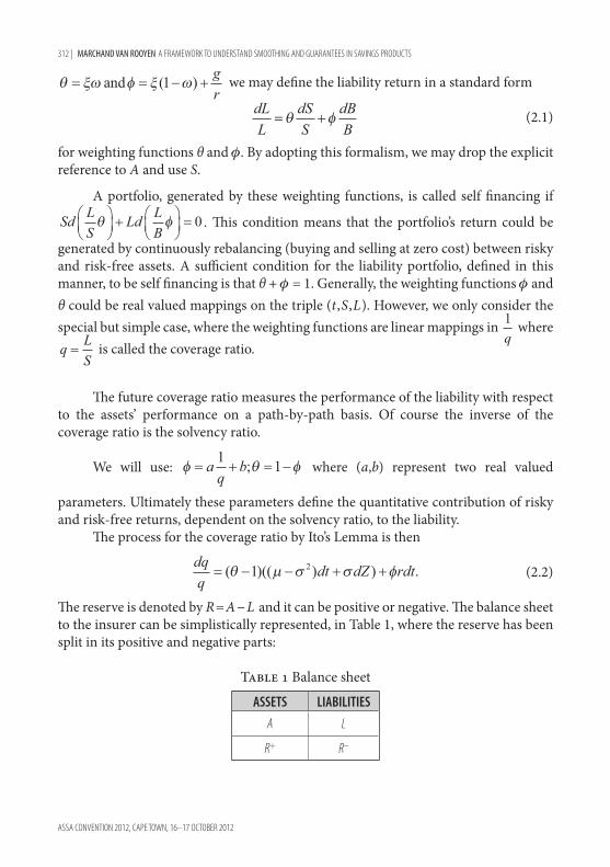
The reserve is denoted by R=A−L and it can be positive or negative. The balance sheet to the insurer can be simplistically represented, in Table 1, where the reserve has been split in its positive and negative parts:

Table 1 Balance sheet

ASSETS LIABILITIESA L

R+ R–



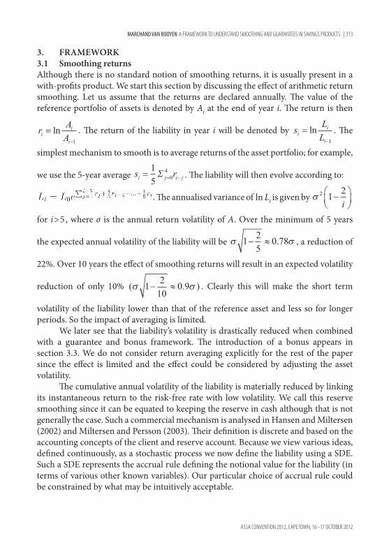
3. FRAmEWORK3.1 Smoothing returnsAlthough there is no standard notion of smoothing returns, it is usually present in a with-profits product. We start this section by discussing the effect of arithmetic return smoothing. Let us assume that the returns are declared annually. The value of the reference portfolio of assets is denoted by Ai at the end of year i. The return is then

r AAii

i

=−

ln1

. The return of the liability in year i will be denoted by s LLii

i

=−

ln1

. The

simplest mechanism to smooth is to average returns of the asset portfolio; for example,

we use the 5-year average s ri j i j= = −

15 0

4Σ . The liability will then evolve according to:

. The annualised variance of ln Li is given by σ 2 1 2−

i

for i>5, where σ is the annual return volatility of A. Over the minimum of 5 years

the expected annual volatility of the liability will be σ σ1 25

0 78− ≈ . , a reduction of

22%. Over 10 years the effect of smoothing returns will result in an expected volatility

reduction of only 10% ( )σ σ1 210

0 9− ≈ . . Clearly this will make the short term

volatility of the liability lower than that of the reference asset and less so for longer periods. So the impact of averaging is limited.

We later see that the liability’s volatility is drastically reduced when combined with a guarantee and bonus framework. The introduction of a bonus appears in section 3.3. We do not consider return averaging explicitly for the rest of the paper since the effect is limited and the effect could be considered by adjusting the asset volatility.

The cumulative annual volatility of the liability is materially reduced by linking its instantaneous return to the risk-free rate with low volatility. We call this reserve smoothing since it can be equated to keeping the reserve in cash although that is not generally the case. Such a commercial mechanism is analysed in Hansen and Miltersen (2002) and Miltersen and Persson (2003). Their definition is discrete and based on the accounting concepts of the client and reserve account. Because we view various ideas, defined continuously, as a stochastic process we now define the liability using a SDE. Such a SDE represents the accrual rule defining the notional value for the liability (in terms of various other known variables). Our particular choice of accrual rule could be constrained by what may be intuitively acceptable.



3.2 Reserve SmoothingWe assume that all assets are held in risky assets, collectively represented by S. We let the liability participate directly in the assets’ returns, and excess reserve is distributed (resp. shortfall is charged) as defined by a mean reverting process. For our purposes a process that pays out excess reserves and recoups for a shortfall over time would be a mean reverting process. In practice, the excess (or shortfall) reserve may be defined in a proportionate way relative to a target solvency ratio. A simple mathematical way to define a mean reverting process is by using an SDE of a special form.

Let us proceed by letting the liability participate in the risky returns by attributing a fraction of risky returns to the liability. Hence the liability will potentially accrue some of the higher expected risky returns. In addition, risky assets in excess of a liability multiple is transferred to the liability at a fixed rate. The liability multiple would be the liability multiplied by target solvency ratio. Conversely, a shortfall to the liability multiple is recouped by reducing the liability return. In other words, we consider the liability where it is defined by the SDE

where 0<ρ≤1 denotes the participation rate, β≈1 denotes the target solvency ratio, and α is the reserve distribution or charging rate. Since R=S−L the reserve then satisfies

Figure 3.1



Clearly the reserve reverts to the level 1 1−

β

S relative to the assets, with reversion

rate αβ (if β close to 1 then 1 1 1− −β

β ). Figure 3.1 illustrates a sample path over

10 years (to construct the example we did not use the continuous time accrual but a discrete time version where the steps are quarterly) where μ=0.09, σ=0.15, ρ=0.6, α=1.5 and β=1.05 for the asset with the corresponding defined liability and reserve as percentage of assets.

Note that the instantaneous variance of the liability is then (ρσ)2 and this may still transfer substantial volatility to the liability. When ρ=0 the instantaneous volatility is 0 and the liability’s only return comes from paying out excess reserves, as represented

by the term α β1q

dt−

. We explore this case next to see what the effective volatility

of the liability would be.Writing the process for the liability in our standard format is

if ρ=0. The solution to

this SDE, after some algebraic manipulation, is

We interpret this formula next. In continuous time, the P&L of holding x units of S at time u would be xdSu and an integral represents the cumulative P&L from trading S. The last integral term of the equation above is of such a form, where the holding in S at time u is 1 1− −( )− −α β( )( )e t u . It means that the return of Lt can be seen as a weighted return of Su; 0<u<t. The volatility of Lt is determined by these weightings where the initial weighting in S is 1 1− −( )−α β( )e t , which is below 100%. The weighting grows to 100% at u=t . This drives the smoothing of returns of S in L. We demonstrate the magnitude of the reduction for different target solvency ratios and reserve payout rates next.

Lt is an Ito Integral and its variance is given by the integral , which is not tractable since S is stochastic.

However, we may obtain an upper bound using Jenson’s inequality. It follows that this integral is bounded above by

Also note that since the variance of St is given by



. Thus the ratio of variance of Lt to St is given by the leading term in brackets and it specifies the volatility reduction as a consequence of reserve smoothing. Figure 3.2 illustrates the upper bound of average annual volatility (the square root of the leading term in brackets divided by t) of Lt as a function of the payout rate α, for σ=0.15 and t=10.

It demonstrates how effective reserve smoothing could be since the standard deviation of L10 could be lower than 4% when the risky asset volatility is 15%. In due course, in section 4, we consider a wide range of strategies and we demonstrate that there are many strategies that lower the terminal variance of L compared to the variance of S.

3.3 Bonus formulaWith-profits funds accrue a guaranteed return with a discretionary bonus, and we develop the logic for a simple vesting bonus over an accrual period. By retaining some of the asset returns in the reserve, a mechanism is required to transfer returns to policyholders. In the previous section, we defined the mechanism using an accrual rule premised on a mean reverting reserve level relative to the asset value.

With-profits returns incorporate two accrual components. One part accrues the guaranteed return. The second component is a vesting bonus based on various factors including: the excess (average) return, current reserves or lack thereof (equivalently the solvency ratio), returns from competing products and expected future market

Figure 3.2



conditions. To the extent that the bonus is dependent on excess returns and the asset liability ratio, we present a formula that represents a vesting bonus.

Since we work discretely over an accrual period, we digress from the continuous time setting briefly (we introduce the discrete time setting in section 4.1). For the moment subscripts will identify the parameter for a particular interval indexed with i. Suppose, by contractual agreement, that there is a guaranteed rate of return g per year. The excess return is max (0,ri+1−g)=(ri+1−g)+. If a fraction ρ of this is added to the return of the liability, then the coverage ratio would become (denoted by the hat)

. This formula reflects that, if the risky returns are below the guaranteed rate the coverage ratio would decrease by g−ri+1. On the other hand, if the risky return exceeds the guarantee rate then the coverage ratio will decrease by (1−ρ)(ri+1−g)>0. In general, is unlikely to be equal to the target coverage ratio. Suppose the fund targets a coverage ratio eβ. To create a situation where the coverage ratio moves closer to the target, the excess return is adjusted upwards or downwards based on the difference between and the target solvency ratio, if at all possible. The adjustment is affected by adding a fraction γ of the difference: . The vesting bonus (excess return and adjustments for coverage ratio) becomes

and liability will then be: . In summary

This bonus formula shows that the policyholder only has upside exposure to the risky return to the extent that the risky return exceeds the guarantee rate by the term (ρ+γ(1−ρ))(ri+1−g). The rest of the bonus, i.e. γ(β−lnqi) reflects additional bonus to the extent that the remaining return (ri+1−g) exceeds the target coverage ratio deficit (lnqi–β). If the coverage ratio is lagging the target then a portion is also taken to reserves.

We would like to compare the accrual mechanism to others and to this end we need to ignore the bonus mechanism (ignore the guarantee rate mechanism defined by the max and g parts). Then the liability return would be (ρ+γ(1−ρ))ri+1+γ(lnqi–β), and in continuous time we could write . This form is analogous to the SDE defining reserve smoothing. The non-guaranteed version of the return can be viewed as that of a portfolio where the asset weightings depend linearly on the solvency ratio.

3.4 Portfolio InsurancePortfolio insurance is a concept that grew from dynamically hedging an option, thereby creating the option payoff, particularly before the Wall Street crash in 1987.



A simple put option dynamic hedging strategy accounts for portfolio insurance at a chosen point in time, which is a significant limitation from a practical point of view. Usually it is applied over a short time horizon which is rolled forward as time passes.

Other strategies that have been used for portfolio insurance include: Constant Proportion Portfolio Insurance (CPPI) (Balder, Brandl & Mahayni, 2009; Boulier & Kanniganti, 1995; Black & Jones, 1987), direct use of options and other derivatives on an ongoing basis found in Variable Annuities (Blamont & Sagoo, 2009), and more recently the definition of dynamic fund protection (Gerber & Pafumi, 2000), which has some similarity to a look-back option but on a contingent notional amount. As the protection becomes more effective the cost of the strategy also increases and it can be too expensive in practice.

For our purposes we define the liability in a way that the policyholder has participation to the upside (to some degree) and less risk on the downside (again to some degree), as opposed to using a CPPI or other portfolio insurance strategy. To this end we take the cue from the definition of CPPI, defined by the SDE

This process protects the portfolio with value A from a floor level, denoted by Ft. The parameter m represents a leverage parameter. If the portfolio value falls to the floor value there would be no exposure to the risky asset and all investments would be in bonds that accrue to the guaranteed maturity value. Of course various additional features are introduced to CPPI from a commercial perspective. The behaviour of a CPPI strategy is well understood and studied. We adapt this approach so that the liabilities follow asset returns to the extent that the liability lags the assets, but accrue at the risk-free rate otherwise to limit the exposure to the insurer.

To this end we modify the strategy as follows. Risky returns accrue proportional to the amount that the liability is behind the assets. In other words the process for the liability will be

(3.1)

for some parameters m>0 and β>0. The parameter m is an exposure leverage parameter and β represents the relative amount that the assets should exceed the liability. Because the implied weightings add up to one, the portfolio is self financing and consequently we know the fair value of Lt to be the initial capital invested L0. The distribution of L appears in Figure 3.3 where m=2, and β=1.05, and it indicates that the liability will perform better than the risky asset on the downside.

We obtained this figure by using the solution of (3.1). To this end choose a=−m and b=1+mβ, in the Appendix. For our strategy m and β are non-negative and therefore 1+mβ≠0. Subsequently we obtain



It is straightforward to verify that, if m>0 and ≥0, then Lt≥0. This is relevant to decide on parameters but this will not be generally true when we move to discrete time. This formula indicates that the liability does not depend on the particular path that the risky assets follow, similar to CPPI. The formula also explains that the liability is the same as a long or short position in the risky asset:

— the leading term shows a long position in St to the amount ,

— assuming that ≥0, the second term shows a non linear short exposure in St, that becomes bigger in size as St becomes smaller, because of the negative power −mβ<0,

— the notional size of this total exposure becomes shorter and bigger in size as St is smaller, dominated by the second term.

If the risky asset underperforms, then the non-linear short exposure in the second term creates some downside out-performance for the liability.

Figure 3.3



3.5 Derivatives and Conceptual ConsiderationsDerivatives’ application to create an investment with downside protection and upside participation are numerous. The difference to the approaches introduced above is that derivatives are defined with a payoff as opposed to an accrual rule. A derivative payoff depends on variables: the asset values at selected times. Examples of such products are Variable Annuities (Blamont & Sagoo, 2009). There is a great deal of similarity with the above concepts however. For example, bonuses that vest would be comparable to a ratcheting strike option – called a Cliquet option. Other option payoffs that are used would include Look-back options and Average-rate options.

In fact, in recent times the trend has been to view the guarantee exposure as a complex and exotic derivative. However, because an insurance product is generally not easily defined by a payoff at a point in time, derivative models for the value of the guarantee are usually implemented as Monte Carlo simulations of the referenced asset values or prices. These valuation, and consequent hedging, models require substantial investment in computational infrastructure as well as ultimately accepting some numerical error due to the slower rates of convergence from the Monte Carlo simulation of long dated and heavily path dependent payoffs. It is also rare that the market value of the asset is computed and reported in a like manner since that belongs to the policyholder. Shareholders bear the burden of the minimum guarantee in the end although some risk sharing may apply.

It is also interesting to ask the question whether it is possible to follow a dynamic asset allocation in such a way that the resulting investment has a guaranteed minimum rate of return with equity upside. This is generally not possible as explored in Kleinow and Willder (2007) and Kleinow (2009).

We indicate structural similarities between smoothing, reserve distribution and portfolio insurance through their weighting functions, in Table 2 below. All these simplistic definitions of a liability accrual rule have portfolio weighting terms that depend linearly on the solvency ratio and include a fixed return component. It is the fixed return component that induces a smoothing of returns of the associated defined liability. When making well-considered choices of parameters, for example as with a bonus formula, the resulting liability may not be self financing and the mark to market of the asset is different to the book value. By using self-financing affine strategies to define the liability we always have the mark to market of the liability equal to the book value and the accrual rule fully defines the liability.

3.6 SummaryWe summarise our conceptual SDE framework in Tables 2 and 3. Table 2 gives a descriptive comparison and Table 3 an algebraic comparison. These tables makes it simple to compare the accrual mechanism defining the liability.

Reserve smoothing differs from the Bonus in the attribution of risky returns, i.e. in the θ component. The structure for the bond return is equivalent. We explore the characteristics of the parametric case, defined in discrete time, in the next section. The



parametric case represents all simple mechanisms of dynamically re-balancing a self-financing portfolio, driven by the solvency ratio.

Table 2 Comparison of accrual logic for different liability definitions

Scheme Bonus Reserve Smoothing CPLI

Mechanism Risky Bond Risky Bond Risky Bond

Fraction (based of liability) X

Fraction re-based to asset level X

Proportional to excess solvency X X X

The balance/self financing X

Table 3 Weighting function comparison

Scheme θ

Bonus ρ γ γβ1q

−

Reserve smoothing pq1

α αβ1q

−

CPLI mqm1

− β − + +mq

m1 1( )β

Parametric − + −aq

b1 1( ) aqb1

+

4. DISCRETE TImE4.1 DefinitionsThere are various options to define the liability in discrete time in the spirit of the continuous time approach. It is also essential to move to discrete time to make it possible to define the bonus and guarantee mechanism properly. We want to fix the weightings over an interval. In general we denote the fixed weightings θi and i using information up to the end of period i. From continuous time (using Ito’s Lemma) we have

If the weightings are fixed over a time interval, then the solution to preceding SDE is



where r ssii

i+

+=

1

1ln . This formula motivates a possible definition of the liability in

discrete time. However, to replicate this liability in reality would require continuous rebalancing and, because we wish to fix the implicit asset weightings in an interval, we do not use this definition. We rather adopt the following definition:

when there is no guarantee. This is well defined regardless of the choice of weightings θi, i. When the liability is self financing, i.e. θi + i = 1, we get

(4.1)

To cater for a guarantee we modify the liability accrual rule as follows. Gρ denotes a guaranteed liability, where the parameter ρ represents the participation ratio, as it is defined

(4.2)

The participation ratio is required so that we may price the guarantee and it represents a reduction in effective notional exposure. For the liability L we have a self-financing portfolio strategy, consequently we have the fair value (also called risk-neutral value) of the liability is its initial value, i.e. the capital initially invested. In mathematical finance, see for example Baxter and Rennie (1996), we write this as , where the expectation EQ refers to the risk neutral expectation (for simple Geometric Brownian Motion this expectation is computed by setting μ=r). However, for a guaranteed liability it is typical that its fair value exceeds the initial investment when the participation level is 100%. That would translate into a loss to the insurer which is not fair. In the analysis that follows we found the participation ratio (with respect to selected parameters) such that the liability’s fair value is equal to the initial investment, i.e. that . We therefore suppress dependency on the participation ratio in the notation below.

We consider weightings in the parametric form that will be linear in 1q :

For practical reasons it will be useful to add constraints on the value of the bond weighting i : bounded from above by u and from below by l:

Unless stated we hence use the constrained parametric weightings with u=1 and l=0, which exclude any leverage.



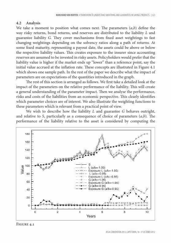
4.2 Analysis We take a moment to position what comes next. The parameters (a,b) define the way risky returns, bond returns, and reserves are distributed to the liability L and guarantee liability G. They cover mechanisms from fixed asset weightings to fast changing weightings depending on the solvency ratios along a path of returns. At some fixed maturity, representing a payout date, the assets could be above or below the respective liability values. This creates exposure to the insurer since accounting reserves are assumed to be invested in risky assets. Policyholders would prefer that the liability value is higher if the market ends up “lower” than a reference point, say the initial value accrued at the inflation rate. These concepts are illustrated in Figure 4.1 which shows one sample path. In the rest of the paper we describe what the impact of parameters are on expectations of the quantities introduced in the graph.

The rest of this section is arranged as follows. We first take a detailed look at the impact of the parameters on the relative performance of the liability. This will create a general understanding of the parameter impact. Then we analyse the performance, risks and costs of the liabilities from an economic perspective. This clearly identifies which parameter choices are of interest. We also illustrate the weighting functions to these parameters which is relevant from a practical point of view.

We wish to describe how the liability L and guarantee G behaves outright, and relative to S, particularly as a consequence of choice of parameters (a,b). The performance of the liability relative to the asset is considered by computing the

Figure 4.1



expectations of L conditional on the terminal value of S: E(LT|ST∈[x ,y]) . We choose to use 5 equi-probable intervals for the terminal state of ST denoted by Ii for i=1,2 ,3 ,4 ,5 :

where F–1 denotes the inverse cumulative probability density function of the Normal distribution. We denote the conditional expectations, using non-italic Roman charac-ters: q− i= for i=1,2 ,3 ,4 ,5 .

Throughout the analysis we used the following parameter values: Starting asset and liability values = 100. The time horizon is 10 years with quarterly rebalancing. The expected asset return is 9% and the risk-free rate is 6%. The guaranteed liability has a guarantee rate of 2% and bonuses are vesting quarterly. The asset returns are subject to an annual volatility of 15%. In summary: S0=L0=100, T=10, δ=0.25, μ=0.09, r=0.06, σ=0.15, and g=0.02.

We digress for a moment and consider the continuous case where the cover ratio q is described by the following SDE:

dq=qθ((r−μ+σ2)dt+σdZ),

with solution (see Appendix)

Its expectation is

This expectation represents the expected performance of the liability with respect to the risky assets. Figure 4.2 illustrates the expected coverage ratio at 10 years as function of the parameters (a,b). Recall that these parameters affect the contribution and the impact of the solvency ratio of risky and risk-free return to the liability’s return. It is easier to understand the impact of changes of these parameters by depicting the expected coverage ratio as it changes for different values of the ratio

ab

, and for different values of a+b. We use the ratio and sum through the rest of our analysis of L and G.

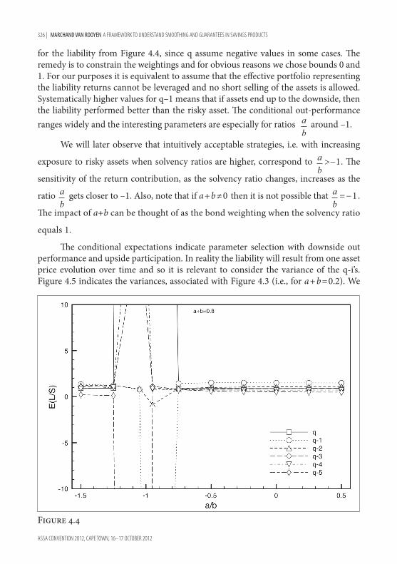
We provide the same illustration for the conditional expectations q−i. The calculation of these values was by Monte Carlo simulation for two cases: a+b=0.2 and a+b=0.8. We used a million sample paths, each with 40 quarterly steps (representing a 10-year holding period), and returns of the risky asset using pseudo random numbers. The calculation was implemented in Matlab using standard functions.

Figures 4.3 and 4.4 observe different behaviour of L with respect to S primarily by different choices of the ratio a

b. Also note that it is possible to realise negative values



Figure 4.3

Figure 4.2



for the liability from Figure 4.4, since q assume negative values in some cases. The remedy is to constrain the weightings and for obvious reasons we chose bounds 0 and 1. For our purposes it is equivalent to assume that the effective portfolio representing the liability returns cannot be leveraged and no short selling of the assets is allowed. Systematically higher values for q–1 means that if assets end up to the downside, then the liability performed better than the risky asset. The conditional out-performance ranges widely and the interesting parameters are especially for ratios a

b around –1.

We will later observe that intuitively acceptable strategies, i.e. with increasing

exposure to risky assets when solvency ratios are higher, correspond to ab

>−1. The

sensitivity of the return contribution, as the solvency ratio changes, increases as the

ratio ab

gets closer to –1. Also, note that if a+b≠0 then it is not possible that ab

=−1.

The impact of a+b can be thought of as the bond weighting when the solvency ratio

equals 1.

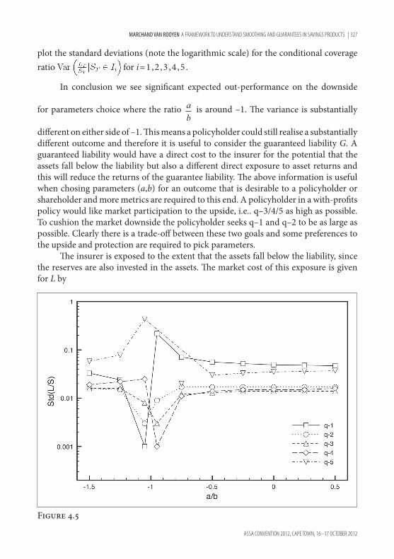
The conditional expectations indicate parameter selection with downside out performance and upside participation. In reality the liability will result from one asset price evolution over time and so it is relevant to consider the variance of the q-i’s. Figure 4.5 indicates the variances, associated with Figure 4.3 (i.e., for a+b=0.2). We

Figure 4.4



plot the standard deviations (note the logarithmic scale) for the conditional coverage ratio for i=1,2 ,3 ,4 ,5 .

In conclusion we see significant expected out-performance on the downside

for parameters choice where the ratio ab

is around –1. The variance is substantially

different on either side of –1. This means a policyholder could still realise a substantially different outcome and therefore it is useful to consider the guaranteed liability G. A guaranteed liability would have a direct cost to the insurer for the potential that the assets fall below the liability but also a different direct exposure to asset returns and this will reduce the returns of the guarantee liability. The above information is useful when chosing parameters (a,b) for an outcome that is desirable to a policyholder or shareholder and more metrics are required to this end. A policyholder in a with-profits policy would like market participation to the upside, i.e.. q–3/4/5 as high as possible. To cushion the market downside the policyholder seeks q–1 and q–2 to be as large as possible. Clearly there is a trade-off between these two goals and some preferences to the upside and protection are required to pick parameters.

The insurer is exposed to the extent that the assets fall below the liability, since the reserves are also invested in the assets. The market cost of this exposure is given for L by

Figure 4.5



where the expectation is taken in the risk neutral measure. This cost is called the Investment Guarantee Reserve (IGR) and Figure 4.6 shows it with respect to different

ratios ab

(we always used an initial coverage ratio of 1, i.e. q0=1). The figure indicates that the lowest IGR results when a+b is smaller and then the ratio has limited impact. For other combinations there is no systematic impact. Note that the IGR for a guaranteed liability can be lower than for a non-guaranteed liability for

ab

around –0.5. Of course the expected return of the guaranteed liability is probably lower than in the non-guaranteed case.

To simplify the decision-making we do not consider the 5 conditional expectations. We pick a level of performance which will define the upside vs downside. In this context we choose this point to reflect a watermark return of 5% by using a level denoted WT=S0e0.05T=164.9 for T=10. Then we define the downside/upside expectations, for example for S, as Sd/u=E(ST|ST</>WT).

We now have all the components to indicate with respect to a wide selection of parameters (a,b) what the performance and risks would be. Tables 4 and 5 give

Figure 4.6



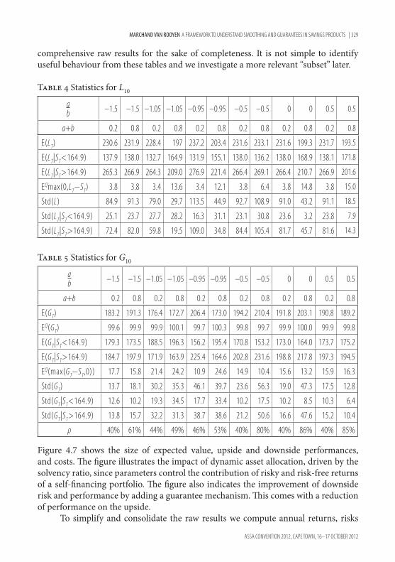
comprehensive raw results for the sake of completeness. It is not simple to identify useful behaviour from these tables and we investigate a more relevant “subset” later.

Table 4 Statistics for L10

ab –1.5 –1.5 –1.05 –1.05 –0.95 –0.95 –0.5 –0.5 0 0 0.5 0.5

a+b 0.2 0.8 0.2 0.8 0.2 0.8 0.2 0.8 0.2 0.8 0.2 0.8

E(LT) 230.6 231.9 228.4 197 237.2 203.4 231.6 233.1 231.6 199.3 231.7 193.5

E(LT|ST<164.9) 137.9 138.0 132.7 164.9 131.9 155.1 138.0 136.2 138.0 168.9 138.1 171.8

E(LT|ST>164.9) 265.3 266.9 264.3 209.0 276.9 221.4 266.4 269.1 266.4 210.7 266.9 201.6

EQmax(0,LT−ST) 3.8 3.8 3.4 13.6 3.4 12.1 3.8 6.4 3.8 14.8 3.8 15.0

Std(L) 84.9 91.3 79.0 29.7 113.5 44.9 92.7 108.9 91.0 43.2 91.1 18.5

Std(LT|ST<164.9) 25.1 23.7 27.7 28.2 16.3 31.1 23.1 30.8 23.6 3.2 23.8 7.9

Std(LT|ST>164.9) 72.4 82.0 59.8 19.5 109.0 34.8 84.4 105.4 81.7 45.7 81.6 14.3

Table 5 Statistics for G10

ab –1.5 –1.5 –1.05 –1.05 –0.95 –0.95 –0.5 –0.5 0 0 0.5 0.5

a+b 0.2 0.8 0.2 0.8 0.2 0.8 0.2 0.8 0.2 0.8 0.2 0.8

E(GT) 183.2 191.3 176.4 172.7 206.4 173.0 194.2 210.4 191.8 203.1 190.8 189.2

EQ(GT) 99.6 99.9 99.9 100.1 99.7 100.3 99.8 99.7 99.9 100.0 99.9 99.8

E(GT|ST<164.9) 179.3 173.5 188.5 196.3 156.2 195.4 170.8 153.2 173.0 164.0 173.7 175.2

E(GT|ST>164.9) 184.7 197.9 171.9 163.9 225.4 164.6 202.8 231.6 198.8 217.8 197.3 194.5

EQ(max(GT−ST,0)) 17.7 15.8 21.4 24.2 10.9 24.6 14.9 10.4 15.6 13.2 15.9 16.3

Std(GT) 13.7 18.1 30.2 35.3 46.1 39.7 23.6 56.3 19.0 47.3 17.5 12.8

Std(GT|ST<164.9) 12.6 10.2 19.3 34.5 17.7 33.4 10.2 17.5 10.2 8.5 10.3 6.4

Std(GT|ST>164.9) 13.8 15.7 32.2 31.3 38.7 38.6 21.2 50.6 16.6 47.6 15.2 10.4

ρ 40% 61% 44% 49% 46% 53% 40% 80% 40% 86% 40% 85%

Figure 4.7 shows the size of expected value, upside and downside performances, and costs. The figure illustrates the impact of dynamic asset allocation, driven by the solvency ratio, since parameters control the contribution of risky and risk-free returns of a self-financing portfolio. The figure also indicates the improvement of downside risk and performance by adding a guarantee mechanism. This comes with a reduction of performance on the upside.

To simplify and consolidate the raw results we compute annual returns, risks



and costs (from Tables 4 and 5) in Table 6. It provides a summary of the economic impact of different accrual rules.

Table 6 Return, Std and IGR for liabilities for a+b=0.2/0.8

a/b L return G return Std L Std G Igr L Igr G

–1.5 8.35%/6.78% 6.06%/5.47% 11.64%/4.76% 2.37%/6.46% .37%/1.28% 1.64%/2.16%

–1.25 8.31%/7.1% 5.95%/5.48% 11.1%/6.98% 3.17%/7.26% .37%/1.14% 1.74%/2.19%

–1.05 8.26%/8.15% 5.68%/5.54% 10.94%/13.96% 5.41%/7.16% .34%/.63% 1.94%/2.11%

–0.95 8.64%/8.46% 7.25%/7.44% 15.13%/14.77% 7.06%/8.46% .33%/.62% 1.04%/.99%

–0.75 8.47%/7.44% 6.82%/7.47% 13.23%/11.26% 4.64%/9.52% .37%/1.25% 1.3%/1.07%

–0.5 8.4%/6.9% 6.64%/7.09% 12.66%/6.86% 3.85%/7.37% .37%/1.38% 1.4%/1.24%

–0.25 8.43%/6.7% 6.56%/6.69% 12.59%/4.37% 3.4%/4.44% .37%/1.4% 1.43%/1.38%

0 8.4%/6.6% 6.51%/6.38% 12.42%/3.02% 3.13%/2.13% .37%/1.4% 1.45%/1.51%

0.25 8.41%/6.54% 6.49%/6.22% 12.45%/2.51% 2.99%/1.29% .37%/1.41% 1.47%/1.62%

0.5 8.4%/6.52% 6.46%/6.12% 12.43%/2.36% 2.9%/1.25% .37%/1.41% 1.48%/1.66%

Figure 4.7



We now wish to focus on a subset of parameters, those where the ratio ab

lies between –1 and 0, and take further steps to consolidate the results in terms of performance ratios.

We identify whether some of the considered liabilities are better suited from a with-profits perspective. Consider the weighting functions, illustrated in Figure 4.8, that result for the indicated choices of parameters a and b.

We see that, for ab

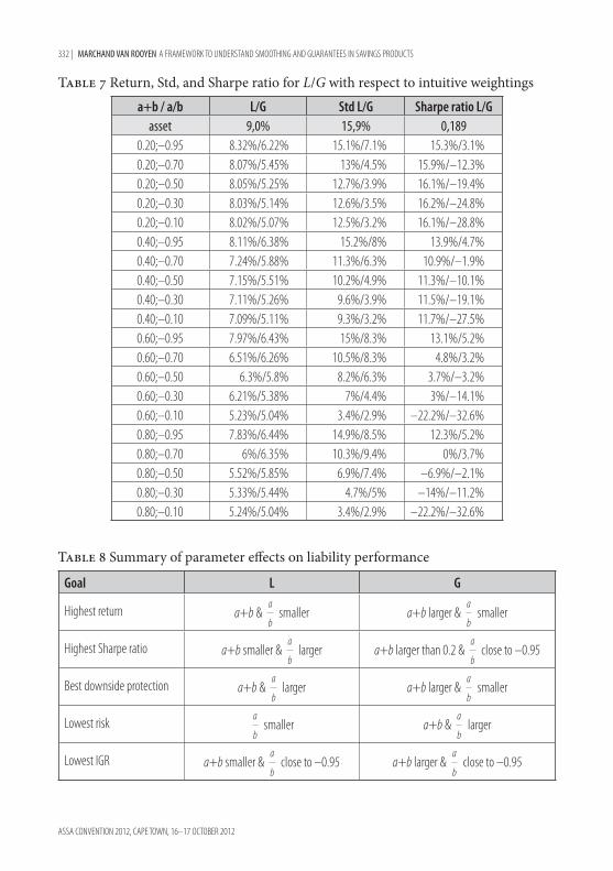
between –1 and 0, we get weighting functions that are intuitive, i.e. the liability return weights the asset return higher for higher solvency ratios. For this subset, corresponding to intuitive with-profits accrual rules, we generated more granular results. Table 7 indicates the resulting returns, volatilities and Sharpe ratios with respect to a wide range of intuitive parameters.

These numbers show that some accrual rules may result in negative Sharpe ratios which one may wish to avoid. They also demonstrate an earlier claim that the volatility of a guaranteed liability is substantially lower. We summarise the high level impact of parameter choices next. Table 8 states the parametric choices that give the optimal choices in respect of returns, economic performance, risk to the policyholder and risk to the insurer.

Figure 4.8



Table 7 Return, Std, and Sharpe ratio for L/G with respect to intuitive weightings

a+b / a/b L/G Std L/G Sharpe ratio L/Gasset 9,0% 15,9% 0,189

0.20;–0.95 8.32%/6.22% 15.1%/7.1% 15.3%/3.1%0.20;–0.70 8.07%/5.45% 13%/4.5% 15.9%/–12.3%0.20;–0.50 8.05%/5.25% 12.7%/3.9% 16.1%/–19.4%0.20;–0.30 8.03%/5.14% 12.6%/3.5% 16.2%/–24.8%0.20;–0.10 8.02%/5.07% 12.5%/3.2% 16.1%/–28.8%0.40;–0.95 8.11%/6.38% 15.2%/8% 13.9%/4.7%0.40;–0.70 7.24%/5.88% 11.3%/6.3% 10.9%/–1.9%0.40;–0.50 7.15%/5.51% 10.2%/4.9% 11.3%/–10.1%0.40;–0.30 7.11%/5.26% 9.6%/3.9% 11.5%/–19.1%0.40;–0.10 7.09%/5.11% 9.3%/3.2% 11.7%/–27.5%0.60;–0.95 7.97%/6.43% 15%/8.3% 13.1%/5.2%0.60;–0.70 6.51%/6.26% 10.5%/8.3% 4.8%/3.2%0.60;–0.50 6.3%/5.8% 8.2%/6.3% 3.7%/–3.2%0.60;–0.30 6.21%/5.38% 7%/4.4% 3%/–14.1%0.60;–0.10 5.23%/5.04% 3.4%/2.9% –22.2%/–32.6%0.80;–0.95 7.83%/6.44% 14.9%/8.5% 12.3%/5.2%0.80;–0.70 6%/6.35% 10.3%/9.4% 0%/3.7%0.80;–0.50 5.52%/5.85% 6.9%/7.4% –6.9%/–2.1%0.80;–0.30 5.33%/5.44% 4.7%/5% –14%/–11.2%0.80;–0.10 5.24%/5.04% 3.4%/2.9% –22.2%/–32.6%

Table 8 Summary of parameter effects on liability performance

Goal L G

Highest return a+b & a

b smaller a+b larger &

a

b smaller

Highest Sharpe ratio a+b smaller & a

b larger a+b larger than 0.2 &

a

b close to –0.95

Best downside protection a+b & a

b larger a+b larger &

a

b smaller

Lowest risk a

b smaller a+b &

a

b larger

Lowest IGR a+b smaller & a

b close to –0.95 a+b larger &

a

b close to –0.95



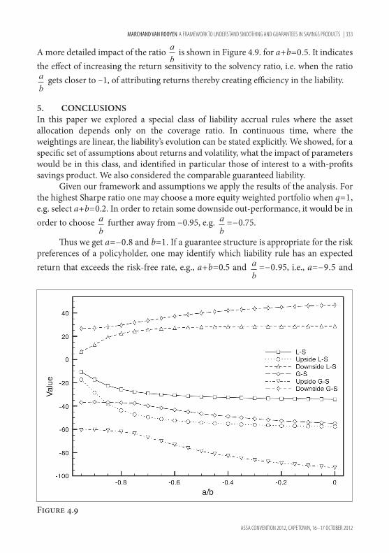
A more detailed impact of the ratio ab

is shown in Figure 4.9. for a+b=0.5. It indicates the effect of increasing the return sensitivity to the solvency ratio, i.e. when the ratio ab

gets closer to –1, of attributing returns thereby creating efficiency in the liability.

5. CONCLuSIONSIn this paper we explored a special class of liability accrual rules where the asset allocation depends only on the coverage ratio. In continuous time, where the weightings are linear, the liability’s evolution can be stated explicitly. We showed, for a specific set of assumptions about returns and volatility, what the impact of parameters would be in this class, and identified in particular those of interest to a with-profits savings product. We also considered the comparable guaranteed liability.

Given our framework and assumptions we apply the results of the analysis. For the highest Sharpe ratio one may choose a more equity weighted portfolio when q=1, e.g. select a+b=0.2. In order to retain some downside out-performance, it would be in order to choose a

b further away from −0.95, e.g. a

b=−0.75.

Thus we get a=−0.8 and b=1. If a guarantee structure is appropriate for the risk preferences of a policyholder, one may identify which liability rule has an expected return that exceeds the risk-free rate, e.g., a+b=0.5 and a

b=−0.95, i.e., a=−9.5 and

Figure 4.9



b=10. These parameters result in a lower IGR and meaningful participation giving a positive Sharpe ratio.

Our analysis above also indicates the following, which could be seen as obvious: the more the liability is defined to be like the risky asset, the lower the IGR and better the expected performance but with less downside out-performance; the performance of our liability with guarantee, when priced to par, materially reduced the participation and thus its expected return.

We emphasize that these conclusions are for our framework and assumptions. In practice other product factors would have an impact on performance and costs and it would be naive to extrapolate the above conclusion as good heuristics in any way. The analysis demonstrates how sensitive the performance could be for parameter choices and structural constraints. Further work, to draw stronger and more general conclusions, should include:

— the impact of assumptions (returns, volatilities and guarantee levels), — possible changes due to return processes more reflective of real markets, and — extending the product setting to allow for additional premiums and benefits to

the policyholder.

In the end, the quest is to identify a combination of liability definition and product features that are demonstrably economically effective for the policyholder and insurer.



REFERENCESBalder, S, Brandl, M & Mahayni, A (2009). Effectiveness of CPPI strategies under discrete-time

trading. Journal of Economic Dynamics and Control 33, 204–20.Baxter, M & Rennie, A (1996). Financial Calculus: An Introduction to Derivative Pricing

September 1996.Black, F & Jones, R (1987). Simplifying portfolio insurance. The Journal of Portfolio Management

14, 48–51.Blamont, D & Sagoo, P (2009). Pricing and hedging variable annuities. Life and Pensions

February 2009.Boulier, JF & Kanniganti, A (1995). Expected performance and risks of various portfolio

insurance strategies. 5th AFIR International Colloquium, 1093–24.Dippenaar, J, Palser, G, Raftensath, L, Van Rensburg, N & Zeeman, A (2007). Smooth bonus

governance. Presented to the Actuarial Society of South Africa, November 2007.Gerber, HU & Pafumi, G (2000). Pricing dynamic investment fund protection. North American

Actuarial Journal 4, 28–36.Hansen, M & Miltersen, KR (2002). Minimum rate of return guarantees: the Danish case.

Scandinavian Actuarial Journal 2002, 280–318.Hibbert, AJ & Turnbull, J (2003). Measuring and managing the economic risks and costs of

with-profits business. British Actuarial Journal 9, 725–77.Kleinow, T & Willder, M (2007). On the effect of management discretion on hedging and fair

valuation of participating policies with interest rate guarantees. Insurance: Mathematics & Economics 40, 445–58.

Kleinow, T (2009). Valuation and hedging of participating life-insurance policies under management discretion. Insurance: Mathematics & Economics 44, 1

Mahayni, A & Schlogle E (2008). The risk management of minimum return guarantees. Business Research 1, 55–76.

Miltersen KR & Persson SA (2003). Guaranteed investment contracts: distributed and undistributed excess return. Scandinavian Actuarial Journal 4, 257–79.



APPENDIx

Solution to when q(θ–1)=–q=–a–bq

We shall find a solution for L by making use of the ratio of liability to assets: . Application of Ito’s lemma yields

If it follows that

which can be integrated explicitly. Thus, if b≠0, then

Noting that we obtain

Finally

When b=0 we have with solution

and

A FRAMEWORK TO UNDERSTAND SMOOTHING - African Agenda

Documents

Transcript of A FRAMEWORK TO UNDERSTAND SMOOTHING - African Agenda