A Framework for Ammonia Supply Chain Optimization ...
13
A Framework for Ammonia Supply Chain Optimization Incorporating Conventional and Renewable Generation Andrew Allman and Prodromos Daoutidis Dept. of Chemical Engineering and Materials Science, University of Minnesota, Minneapolis, MN 55455 Douglas Tiffany Dept. of Applied Economics, University of Minnesota, Saint Paul, MN 55108 Stephen Kelley Humphrey School of Public Affairs, University of Minnesota, Minneapolis, MN 55455 DOI 10.1002/aic.15838 Published online July 31, 2017 in Wiley Online Library (wileyonlinelibrary.com) Ammonia is an essential nutrient for global food production brought to farmers by a well-established supply chain. This article introduces a supply chain optimization framework which incorporates new renewable ammonia plants into the conventional ammonia supply chain. Both economic and environmental objectives are considered. The framework is then applied to two separate case studies analyzing the supply chains of Minnesota and Iowa, respectively. The base case results present an expected trade-off between cost, which favors purchasing ammonia from conventional plants, and emissions, which favor building distributed renewable ammonia plants. Further analysis of this trade-off shows that a carbon tax above $25/t will reduce emissions in the optimal supply chain through building large renewable plants. The importance of scale is emphasized through a Monte Carlo sensitivity analysis, as the largest scale renewable plants are selected most often in the optimal supply chain. V C 2017 American Institute of Chemical Engineers AIChE J, 63: 4390–4402, 2017 Keywords: supply chain optimization, distributed ammonia production, wind power, green fertilizer Introduction Ammonia is one of the most essential chemicals existing today. Without it, there would be no way to ensure the nitro- gen levels required to feed the growing human population. Anhydrous ammonia, a chemical which is 82% nitrogen, is often directly injected into the ground through a stake for use as fertilizer. Ammonia also has many other uses, for example as a precursor to nitrogenous commodity chemicals, as a chemical-based storage of energy, 1 as a way to store hydrogen as a liquid at reasonable temperatures and pressures, 2 and as a liquid fuel. 3 Clearly, demand for ammonia will only continue to grow in the future. 4 The Haber-Bosch process revolutionized the ammonia industry on its discovery in the early 20th century. This pro- cess, however, requires hydrogen as an input. At present, this hydrogen is typically obtained from fossil fuels, using pro- cesses such as steam reforming of methane or coal gasifica- tion. 5 This presents two key sustainability issues: first, ammonia production presents an ever-present and increasing demand on a finite fossil fuel supply, and second, ammonia production contributes to global greenhouse gas emissions, which are believed to be an important factor underlying anthropogenic climate change. Thus, without the introduction of new processes, ammonia cannot be produced at the levels required to supply the growing human population in a sustain- able manner. Motivated by these concerns, a first of its kind pilot scale ammonia plant was recently built at the West Central Research and Outreach Center at the University of Minnesota. This plant produces the hydrogen required for ammonia through wind-powered electrolysis of water. The technology, with a flowsheet depicted in Figure 1, has been proven at the pilot scale. 6 In general, such wind-powered plants will likely be built at a smaller scale than their conventional counterparts which exist at scales as large as 2 million tons per year. 7 Although existing ammonia production is highly centralized, demand for nitrogen fertilizer is distributed all across the country, as shown in Figure 2. 8 This figure shows the acreage of farms growing corn, one of the highest ammonia demand- ing crops. Other critical crops requiring high amounts of ammonia as a source of nitrogen include wheat, barley, oats, and cotton. As such, it seemingly would make more sense to produce ammonia at a smaller scale and in a more distributed fashion to better match supply and demand. In theory, any renewable energy source could be used to power this new renewable ammonia production process. How- ever, Figure 3 can shed some light on why wind is the ideal This contribution was identified by Sipho Ndlela (Owens Corning) as the Best Presentation in the session “Distributed Chemical and Energy Processes for Sus- tainability” at the 2016 AIChE Annual Meeting in San Francisco. Correspondence concerning this article should be addressed to P. Daoutidis at [email protected]. V C 2017 American Institute of Chemical Engineers 4390 AIChE Journal October 2017 Vol. 63, No. 10
Transcript of A Framework for Ammonia Supply Chain Optimization ...

A Framework for Ammonia Supply Chain OptimizationIncorporating Conventional and Renewable Generation
Andrew Allman and Prodromos DaoutidisDept. of Chemical Engineering and Materials Science, University of Minnesota, Minneapolis, MN 55455
Douglas TiffanyDept. of Applied Economics, University of Minnesota, Saint Paul, MN 55108
Stephen KelleyHumphrey School of Public Affairs, University of Minnesota, Minneapolis, MN 55455
DOI 10.1002/aic.15838Published online July 31, 2017 in Wiley Online Library (wileyonlinelibrary.com)
Ammonia is an essential nutrient for global food production brought to farmers by a well-established supply chain. Thisarticle introduces a supply chain optimization framework which incorporates new renewable ammonia plants into theconventional ammonia supply chain. Both economic and environmental objectives are considered. The framework isthen applied to two separate case studies analyzing the supply chains of Minnesota and Iowa, respectively. The basecase results present an expected trade-off between cost, which favors purchasing ammonia from conventional plants,and emissions, which favor building distributed renewable ammonia plants. Further analysis of this trade-off shows thata carbon tax above $25/t will reduce emissions in the optimal supply chain through building large renewable plants.The importance of scale is emphasized through a Monte Carlo sensitivity analysis, as the largest scale renewable plantsare selected most often in the optimal supply chain. VC 2017 American Institute of Chemical Engineers AIChE J, 63:
4390–4402, 2017
Keywords: supply chain optimization, distributed ammonia production, wind power, green fertilizer
Introduction
Ammonia is one of the most essential chemicals existing
today. Without it, there would be no way to ensure the nitro-
gen levels required to feed the growing human population.
Anhydrous ammonia, a chemical which is 82% nitrogen, is
often directly injected into the ground through a stake for use
as fertilizer. Ammonia also has many other uses, for example
as a precursor to nitrogenous commodity chemicals, as a
chemical-based storage of energy,1 as a way to store hydrogen
as a liquid at reasonable temperatures and pressures,2 and as a
liquid fuel.3 Clearly, demand for ammonia will only continue
to grow in the future.4
The Haber-Bosch process revolutionized the ammonia
industry on its discovery in the early 20th century. This pro-
cess, however, requires hydrogen as an input. At present, this
hydrogen is typically obtained from fossil fuels, using pro-
cesses such as steam reforming of methane or coal gasifica-
tion.5 This presents two key sustainability issues: first,
ammonia production presents an ever-present and increasing
demand on a finite fossil fuel supply, and second, ammonia
production contributes to global greenhouse gas emissions,
which are believed to be an important factor underlying
anthropogenic climate change. Thus, without the introduction
of new processes, ammonia cannot be produced at the levels
required to supply the growing human population in a sustain-
able manner.Motivated by these concerns, a first of its kind pilot scale
ammonia plant was recently built at the West Central Research
and Outreach Center at the University of Minnesota. This
plant produces the hydrogen required for ammonia through
wind-powered electrolysis of water. The technology, with a
flowsheet depicted in Figure 1, has been proven at the pilot
scale.6 In general, such wind-powered plants will likely be
built at a smaller scale than their conventional counterparts
which exist at scales as large as 2 million tons per year.7
Although existing ammonia production is highly centralized,
demand for nitrogen fertilizer is distributed all across the
country, as shown in Figure 2.8 This figure shows the acreage
of farms growing corn, one of the highest ammonia demand-
ing crops. Other critical crops requiring high amounts of
ammonia as a source of nitrogen include wheat, barley, oats,
and cotton. As such, it seemingly would make more sense to
produce ammonia at a smaller scale and in a more distributed
fashion to better match supply and demand.In theory, any renewable energy source could be used to
power this new renewable ammonia production process. How-
ever, Figure 3 can shed some light on why wind is the ideal
This contribution was identified by Sipho Ndlela (Owens Corning) as the BestPresentation in the session “Distributed Chemical and Energy Processes for Sus-tainability” at the 2016 AIChE Annual Meeting in San Francisco.
Correspondence concerning this article should be addressed to P. Daoutidis [email protected].
VC 2017 American Institute of Chemical Engineers
4390 AIChE JournalOctober 2017 Vol. 63, No. 10

renewable source to choose.9 In this figure, it is apparent thatthere is significant overlap between the areas with high windpotential and the areas with high ammonia demand in theUnited States. This overlap also occurs in other parts of theworld, such as in Europe where many high potential windareas overlap with high wheat producing locations. In addi-tion, many of the areas with high wind potential are located inrural locales with low population density. As such, this energyis often referred to as “stranded” energy: energy located toofar away from major population centers to be useful withoutincurring substantial transmission costs and losses. Distributedrenewable ammonia production provides a use for thisstranded energy, as it can be used directly onsite to produceammonia, a product that is needed in these rural areas contain-ing a high density of crops requiring anhydrous ammonia orother nitrogen fertilizer.
This article addresses two key questions concerning newrenewable ammonia plants: Can such a renewable plant be
economically competitive with existing conventional plants,and if so, at what scale are the plants competitive? To this end,
the remainder of this article proposes a general framework foranalyzing both conventional and renewable plants within the
ammonia supply chain, and is structured as follows. First,
some background is presented that reviews existing research
on sustainable supply chains and summaries the current state
of the ammonia supply chain. Next, the general mathematical
optimization framework is introduced. We then present some
preliminary data that will be used for the analysis of two case
studies, which look at the ammonia supply chains of the states
of Minnesota and Iowa, respectively. The results of these case
studies are discussed in the following section. Finally, some
concluding remarks and avenues for future work are
presented.
Background
Supply chains consist of networks of material and informa-
tion flows between different facility nodes.10 The nodes often
include suppliers, manufacturers, storage and distribution cen-
ters, and consumers, while the flows can occur through many
different means of transportation, including trucks, barges,
ships, planes, trains, and pipelines. Supply chain optimization,
then, involves determining the best configuration of nodes and
flows that will minimize a certain objective. There are many
possible objectives that one could consider, but in the context
of sustainable supply chains, typically a combination of
Figure 1. Process flowsheet for novel renewableammonia system built in Morris, MN.
Figure 2. Amount of farmland used for corn production by county in the United States.8
Figure 3. Wind resources in the United States.9
AIChE Journal October 2017 Vol. 63, No. 10 Published on behalf of the AIChE DOI 10.1002/aic 4391

economic, environmental, and social metrics, the so called“three pillars” of sustainability, are used.11,12
Supply chain optimization is of critical importance to indus-
try and is particularly useful for new or expanding industriesto understand, for example, how and where additional capacityintegrates with established production. In the following para-
graphs, we briefly review the use of supply chain optimizationapplied to several emerging renewable chemical industries.The most prevalent of these renewable chemical supply chains
involve biofuels and biochemicals. The optimal design of bio-fuel supply chain networks considering uncertainties in vari-ous key parameters, such as local demand, market prices, and
process yields, has been analyzed using a Monte Carloapproach to global sensitivity analysis.13 Other previous workdeveloped a generic framework for a bioethanol supply chain
and applied this over a nine-state region in the upper mid-west.14 This work was extended to allow for selection between
multiple biomass processing technologies as well as take intoaccount existing corn biofuel plants in the analysis.15 Theimplementation of distributed biofuel production has been
examined via a novel small scale biodiesel production facilityto satisfy local fuel demands in the greater London region.16
Additional previous research has incorporated a multiobjective
optimization of cellulosic biofuel supply chains, using a lifecycle analysis that simultaneously considered economic, envi-ronmental, and social objectives.17 This work was extended to
analyze bioelectricity, instead of biofuel, using a similar multi-objective optimization with life cycle analysis approach.18 Abiofuel supply chain which incorporates existing petroleum
infrastructure has also been previously studied, showing thatincorporating existing petroleum production facilities andpipelines into the biofuel supply chain can result in a reduction
of cost.19
Biofuels are not the only renewable chemical considered insupply chain optimization. Hydrogen supply chains consider-
ing both environmental and economic objectives have beeninvestigated, which assume vehicle end use and different pro-duction, storage, and transportation technologies.20 The sugar
supply chain has also been considered in addition to bioetha-nol, as both are potential products of sugarcane.21 A largescale carbon dioxide supply chain has been proposed to ana-
lyze carbon capture, storage, and sequestration and identifyhow best to reduce carbon emissions and utilize carbon diox-ide for profits.22 Ammonia supply chains, which we consider
in this work, have received little attention, in large partbecause conventional ammonia production is a well-established technology. One study considered ammonia as a
potential future energy carrier by taking into account the entireammonia supply chain; however, this study focused on tech-
noeconomic analysis rather than supply chain optimization.23
An additional study considered ammonia as part of a supplychain optimization of a large-scale petrochemical complex,
most of which is used as a precursor to urea production.24
In this work, we seek to develop a supply chain optimiza-tion model which analyzes an ammonia supply chain consider-ing both existing conventional production and new production
with renewably generated hydrogen (“renewable production”)at candidate locations with existing wind capacity. In thissense, supply chain optimization is used here as a tool to pro-
vide a complete comparison of the economic and environmen-tal costs of conventional vs. renewable ammonia production.The traditional ammonia supply chain consists of centralized
conventional plants where ammonia is produced at large
quantities, transported, typically by rail or pipeline, to local
distribution centers, and then further transported by truck to
local consumers.25 This work considers the possibility of
introducing local renewable ammonia plants into the tradi-
tional supply chain. Because these plants are being built
locally, they can bypass the distribution centers and ship
directly to the consumer, using either onsite storage or assum-
ing the end user has sufficient storage. The remainder of this
article develops and uses an optimization formulation to com-
pare renewable and conventional ammonia production within
the supply chain.
Problem Formulation
In this section, an optimization framework is developed that
considers the existing ammonia supply chain and decides if
and where to build renewable plants among candidate location
sites, as well as how to transport ammonia through the supply
chain. The formulation uses steady-state mass balances thr-
oughout the supply chain; in practice, this would be accom-
plished through adequate storage at production, distribution,
and end use nodes. Ammonia can be purchased from existing
conventional plants and then transported to one of the ammo-
nia distribution centers. The total ammonia purchased from a
conventional site may not exceed its maximum allowable
value np
XD
d51
yp;d � np 8p (1)
where yp;d is ammonia shipped from a conventional plant p to
a distribution center d. From the distribution centers, ammonia
is then further transported to local demand sites. At each distri-
bution site, there is a mass balance for ammonia: distribution
centers cannot ship out more ammonia than they receive from
conventional plants
XP
p51
yp;d2XM
m51
yd;m � 0 8d (2)
where yd;m is the amount of ammonia shipped from a distribu-
tion center d to a final demand site m. Local ammonia
demands can also be met by building a new renewable plant.
If this occurs, the plant capacity built (xr) may not exceed its
maximum allowable value nr
xr � nr 8r (3)
As the renewable plant candidate sites are distributed and
local, there is no need to transport this renewable ammonia to
a distribution center; instead, it may be transported directly to
the demand sites. Again, an ammonia mass balance must hold
at each renewable plant, as the plant cannot ship out more
ammonia than it produces
xr2XM
m51
yr;m � 0 8r (4)
where yr;m is the amount of ammonia shipped from a renew-
able site r to a final demand site m. Regardless of whether
renewably or conventionally produced ammonia is used to
satisfy local demand, this demand (dm) must be satisfied at
every demand site in the supply chain
4392 DOI 10.1002/aic Published on behalf of the AIChE October 2017 Vol. 63, No. 10 AIChE Journal

XD
d51
yd;m1XR
r51
yr;m � dm 8m (5)
Lastly, all decision variables must be nonnegative, as back-wards flows are not allowed in the supply chain, and it makesno physical sense to built a plant with negative capacity
x; y � 0 8d;m; p; r (6)
Equations 1–6 provide physical constraints to the supply chainoptimization.
To complete the optimization framework, an objective func-tion is required. It is important for sustainable supply chains toconsider both economic and environmental concerns. Usingmultiobjective optimization techniques, such as the epsilon con-straint method,26 objectives relating to both can be accountedfor. First, an economic objective can be considered by examin-ing the annualized cost of operating the supply chain
cost5XR
r51
XU
u51
qu
hxr
v
� �cu� �
1rxr
!1XR
r51
XM
m51
sr;myr;m
1XP
p51
XD
d51
ðsp;d1apÞyp;d1XD
d51
XM
m51
sd;myd;m
(7)
where qu is the reference capital cost of a unit in the
renewable plant, cu is the capacity exponent of that unit, his the scaled plant lifetime, using a 20-year NPV formula-
tion with a 7% discount rate, v is the reference renewable
plant capacity corresponding to the reference capital cost, ris the operating cost factor for a new renewable plant, si;j
are transportation costs of moving ammonia from i to j,and ap is the cost of purchasing ammonia from conven-
tional plant p. This is the overall supply chain cost, which
consists of terms including the annualized capital cost of
building new renewable ammonia plants, the operating
costs of these new renewable plants, the cost of transport-
ing ammonia through the supply chain, and the cost of pur-
chasing ammonia from conventional plants, respectively. It
is important to note here that a nonlinearity is present in
the capital cost term due to economies of scale. The objec-
tive function also considers that the economies of scale
may differ among units within the renewable plant; for
example, electrolyzer units may not scale as well as the
ammonia reactor.An environmental objective is also considered by account-
ing for the annual amount of carbon dioxide produced from
the ammonia supply chain
Figure 4. Existing ammonia pipelines in the United States.25
AIChE Journal October 2017 Vol. 63, No. 10 Published on behalf of the AIChE DOI 10.1002/aic 4393

emissions5XP
p51
XD
d51
ð�p;d1gpÞyp;d1XD
d51
XM
m51
�d;myd;m
1XR
r51
XM
m51
�r;myr;m
(8)
where �i;j are the emissions resulting from transporting ammo-
nia from i to j, and gp are the emissions resulting from the
production of ammonia at conventional plant p. These are the
overall supply chain emissions, which consist of terms in-
cluding the emissions resulting from transporting ammonia
throughout the supply chain, as well as from conventional
ammonia production, respectively. The emissions function
assumes that all of the power required for renewable ammonia
production is obtained from either direct or stored wind power,
and as such, renewable ammonia production has no associated
carbon emissions.With the economic and environmental objectives defined,
the supply chain optimization framework is complete. This
formulation is a nonconvex nonlinear program (NLP) due sim-
ply to the capital cost term, as the capacity exponent cu will
typically take values less than 1 due to economies of scale.
The formulation could in theory be transformed to a mixed
integer linear program (MILP) if only the economic objective
is considered, as the economies of scale would dictate always
building a plant to its maximum capacity if built. However,
the presence of the second, environmental, objective, means
that in some cases the optimization will decide to build new
renewable plants that are smaller than what is allowed to
decrease transportation emissions. The optimization model
can be solved to global optimality for problems with a small
number of variables or tight known variable bounds by, for
example, using the BARON solver.27
Case Study Preliminaries
To demonstrate the utility of the proposed framework, it is
applied to two separate case studies, analyzing the ammonia
supply chains of Minnesota and Iowa, respectively. Note that
the supply chain framework defined in the previous section
allows for system boundaries as large or small as one would
like. The choice of Minnesota and Iowa, is made because even
though they are neighboring states, they have significant dif-
ferences that make looking at each of the respective supply
chains a worthwhile exercise as specified below. First, as
shown in Figure 4, Iowa has more ammonia pipeline connec-
tions than does Minnesota. Because of this, there is also a
greater number of distribution centers in Iowa, as shown in
Figure 5. Figure 5 also shows agricultural ammonia demand at
a county level for each state. This demand was calculated
using crop planted area data for three major regionally grown
crops: corn and wheat, which have a high demand for ammo-
nia, and soybeans, whose demand is much less.28,29 Reported
data for the average ammonia consumption per area for each
crop was then used to convert this agricultural use to an
ammonia demand.30 Looking at Figure 5, it is apparent that
Iowa has a larger, more geospatially homogeneous demand for
ammonia than Minnesota.Ammonia can be purchased from any of the existing con-
ventional ammonia plants shown in Figure 67 at a nominal
market price of $717/ton.31 Depending on whether the existing
plant uses coal or natural gas as its source for hydrogen, the
related CO2 emissions from purchasing this ammonia are 3.8
or 1.6 t CO2/t NH3, respectively.32 For each plant, a maximum
Figure 5. Ammonia demand and distribution centers in Minnesota (left) and Iowa (right).28–30
Figure 6. Existing conventional ammonia plants con-sidered in this study, with Minnesota andIowa highlighted in gray.7
4394 DOI 10.1002/aic Published on behalf of the AIChE October 2017 Vol. 63, No. 10 AIChE Journal

amount of ammonia allowed for purchasing was determinedbased on the capacity of each plant scaled down based on howfar away such plant is from the area of interest, since conven-tional plants would presumably be supplying other areas anddemands as well. Ammonia purchased from the conventionalplants can be supplied to existing distribution by either pipe-line, rail, or truck. Table 1 gives the maximum purchaseparameters and transport connections for each conventionalammonia plant. Note that the maximum purchases given arefor Minnesota, and Iowa maximum purchases are assumed tobe 50% higher due to its larger demand. Truck transport is notincluded in this table, but is the default mode of transportbetween conventional plants and distribution centers if pipe-line and rail transport are unavailable. Ammonia is then trans-ported by truck from either distribution centers or newrenewable plants to local demand sites, which in this casestudy are assumed to be cities located near the centers of eachcounty with ammonia demand, as shown in Figure 5.
Truck transportation costs and emissions were deter-mined assuming the use of diesel fuel with fuel economy of2.13 km/L, a fuel cost of $0.93/L, fuel emissions of 2.68 kgCO2/L, a single tanker capacity of 17 t,25 and a truck driverwage of $22/h.33 Driving distances and times were found usingthe Google Maps distance matrix API.34 Pipe transportationcosts were determined assuming a piping energy requirementof 185 kJ/kg,25 an electricity cost of $0.08/kWh, and emissionsof 0.98 kg CO2/kWh, the average from coal power plants.35
An additional distance-based pipeline fee is added based onexisting data adjusted for inflation.25 Lastly, rail transportcosts and emissions use the same fuel data as for truck trans-port, with a fuel economy of 204 km-t/L and an additional flatfee based on existing data adjusted for inflation.25
The candidate locations for new renewable ammonia plantsare shown in Figure 7. These candidate sites are cities withnearby existing wind capacity:36 this case study assumes that anew renewable plant would partner with this existing capacityrather than build new wind turbines, to avoid introducing
additional capital costs in the economic analysis. It is further
assumed that a maximum of 37% of the rated wind capacity
could be used for the new ammonia plant, consistent with typi-
cal capacity factors for wind power, at a conversion rate of
1191 t/y/MW, a value obtained from runs of the pilot plant.
For example, these parameters imply that a candidate location
with a 15MW wind farm will be able to support a renewable
plant no larger than 6610 t/y. It is important to note that for
model generality, this capacity factor was assumed constant
for all locations, although in reality it will be a function of
both turbine design and location. From Figure 7, it is evident
that Iowa also has a larger average maximum renewable plant
size in comparison to Minnesota. Comparing Figures 5 and 7,
it is easy to see the overlap between locations of high ammo-
nia demand and high wind potential, presenting the possibility
of ammonia production at a local scale rather than importing
the ammonia from out of state.Economic parameters for the new renewable plants are
obtained from the pilot plant data obtained from the WCROC
facility and are summarized below. From this facility, a total
capital cost of $2.6MM is obtained at a reference capacity of
26.28 t/y. Of this capital cost, 57% is from the ammonia reac-
tor and related components, 28% is from the electrolyzer and
related components, and the remaining 15% is from the air
separation unit and related components. It is further assumed
that a larger, more cost efficient electrolyzer is used in the new
renewable plants in comparison to the pilot plant, giving a
25% cost reduction for this unit due to electrolyzer economies
of scale for sizes up to 2MW. Beyond this scale-up, however,
electrolyzer economies of scale are not as favorable as the rest
of the plant,37 and as such capacity exponents of 0.67, 0.67,
and 0.85 are assumed for the ammonia, nitrogen, and hydro-
gen units, respectively. This capital cost is annualized using an
NPV formulation that assumes a 20-year plant lifetime with
7% annual discount rate. In addition, an operating cost for
operating the new renewable plant of $308/t is applied that
Table 1. Maximum Purchases and Supply Chain Connectivity for Each Conventional Ammonia Plant Considered
Conventional Pipeline MaximumPlant Rail Connections Connections Purchase (t/y)
Beulah, ND Glenwood, Garner, N/A 150,000Spencer, Sloan
Regina, SK Glenwood, Garner, N/A 50,000Spencer, Sloan
Medicine Hat, AB Glenwood, Garner, N/A 300,000Spencer, Sloan
Creston, IA N/A Mankato, Garner 10,000Spencer, Ft. MadisonWashington,Marshalltown
Coffeyville, KS N/A Mankato, Sloan 100,000Verdigris, OK N/A Mankato, Sloan 120,000Woodward, OK N/A Mankato, Sloan 100,000Yazoo City, MS Rosemount, Ft. N/A 50,000
Madison, Washington,Marshalltown
Beaumont, TX Rosemount, Ft. N/A 30,000Madison, Washington,Marshalltown
Geismar, LA Rosemount Garner, Spencer, Ft. 40,000Madison, WashingtonMarshalltown
Lima, OH Rosemount, N/A 40,000Washington,Marshalltown
AIChE Journal October 2017 Vol. 63, No. 10 Published on behalf of the AIChE DOI 10.1002/aic 4395

takes into account energy costs ($294/t), labor, and mainte-nance ($14/t).
Results and Discussion
Base case results
For both the Iowa and Minnesota supply chains, the optimi-zation model was solved using the BARON optimizer inGAMS. For the Minnesota supply chain, the model consistedof 2,522 variables and 152 constraints, while for the Iowa sup-
ply chain, the model consisted of 3,262 variables and 170 con-straints. The model returned the economic optimal solution in4.67 s for the Iowa supply chain and 2.64 s for the Minnesotasupply chain. The low CPU-times can be attributed to the factthat the problem is mostly linear except for one concave objec-
tive, and that upper and lower bounds on all variables areknown due to the mass balances within the supply chain. Themodel solved the problem to a 1029 relative optimality gapusing an Intel Core i7 3.40 GHz 64 bit processor. A tight opti-
mality tolerance is used to ensure that all variables whichshould be zero are not small non-zero values in the solution;the fast solution times confirmed that this choice did not havea major effect on performance.
For the base case parameters, the annual cost of providing
ammonia for the Minnesota supply chain in the economicallyoptimal case was $426 MM/y, or an average consumer cost of$825/t NH3. For the Iowa supply chain, the optimal annualizedcost was $600 MM/y, or an average consumer cost of $827/tNH3. The resulting supply chain emissions in the cost optimal
case were 1.38�106 t/y and 1.70�106 t/y for Minnesota andIowa, respectively. In both cases, the economic base casedecided to build no new ammonia plants, and instead pur-chased all ammonia from conventional plants. The slightly
higher average consumer costs in the Iowa supply chain aredue to its higher demand, which needed to be met by purchas-ing ammonia from plants that were located further away fromIowa, incurring slightly higher transportation costs.
Figure 8 shows the base case economic optimal supply
chains for Minnesota and Iowa. In both states, all of the avail-able distribution centers are used to supply the state’s ammo-nia demand. Although the Minnesota supply chain requiresmore in-state transportation than Iowa due to its fewer distri-bution centers, transportation costs take up about the same
amount of the total costs, about 13%, for both states. This isbecause Iowa sees additional transportation costs due to
requiring ammonia from further away conventional plants tomeet its larger demand. While both states choose to purchaseammonia from the midwestern conventional plants in Iowa,North Dakota, Kansas, Oklahoma, and Ohio, the Iowa supplychain purchases extra ammonia from the southern plants inLouisiana and Mississippi, while the Minnesota supply chaininstead uses the Canadian plants in Alberta and Saskatchewan.
The base case was further analyzed by applying the environ-mental objective function. For Minnesota, the environmentallyoptimal solution gave a supply chain cost of $620 MM/y, 46%more than the economically optimal cost, and emissions of
Figure 7. Candidate locations for new renewable ammonia plants considered in the study.36
Figure 8. Base case economic optimal supply chainsfor Minnesota (top) and Iowa (bottom).
4396 DOI 10.1002/aic Published on behalf of the AIChE October 2017 Vol. 63, No. 10 AIChE Journal

6740 t/y. Averaged over the total ammonia demand, this equa-
tes to a consumer cost of $1200/t NH3 with related emissions
of 0.0131 t CO2/t NH3. For Iowa, the environmentally optimal
solution gave a supply chain cost of $860 MM/y, 43% more
than the economically optimal cost, and emissions of 4490 t/y.
Averaged over the total ammonia demand, this equates to a
consumer cost of $1190/t NH3 with related emissions of
0.00619 t CO2/t NH3. In both cases, the environmentally opti-
mal solution returned a supply chain that obtained ammonia
only from building new renewable plants, and these plants
were highly distributed to minimize transportation, which is
the only cause of emissions in this case. Additionally, the
resulting emissions were three orders of magnitude lower in
the environmentally optimal solution than in the economically
optimal solution, implying that emissions from hydrogen pro-
duction are the key source of emissions in the ammonia supply
chain. As Iowa has more candidate locations that are close to
the counties with high ammonia demand, the optimal emis-
sions for Iowa are less than those of Minnesota. However, for
both states, the emissions in the environmentally optimal case
are multiple orders of magnitude smaller than the emissions in
the economically optimal case. A pictorial representation of
the supply chain solution for the environmentally optimal case
is omitted here for brevity.Using the results obtained from the purely economically or
environmentally optimal solutions, a Pareto front comparing
the trade-offs of these two objectives was obtained using the
epsilon constraint method. The results are shown in Figure 9.
Note that initially, the Pareto front for the Iowa supply chain
drops at a steeper rate than that of the Minnesota supply chain.
This indicates that renewable plants are closer to being cost
competitive in Iowa than they are in Minnesota, a result of
Iowa having larger existing wind plants, and as such, larger
capacity candidate renewable plant sites. In both cases, the
Pareto front (from left to right on Figure 9) first sees a region
where a large amount of emissions reduction is achieved with
relatively little cost increase, indicating a switch from purchas-
ing ammonia from conventional sites to building new renew-
able plants. However, at higher costs, only a very small
emissions reduction is occurring for a larger cost increase and
the Pareto front is essentially flat. At this point, no more
ammonia is being purchased from conventional plants, and the
emission reductions seen are a result of building smaller scale
renewable plants in a distributed fashion, reducing emissions
from in-state transportation. Similar arguments account for the
non-smooth nature of the Pareto front; jumps in cost occur
when emissions are reduced by building a new renewable
plant at its maximum capacity, while more gradual cost
changes indicate that emissions are reduced by changing how
ammonia is transported.
Carbon tax sensitivity
Multiobjective optimization showed that starting at the eco-
nomically optimal solution, there is potential for a high
amount of emissions reduction for little additional cost. This
implies that economic incentives, such as a carbon tax, may be
effective in promoting new renewable plants to be present in
the economically optimal solution. This is tested by optimiz-
ing a new function which takes into account the supply chain
costs previously considered, as well as the supply chain
emissions:
new cost5cost1fðemissionsÞ (9)
where f is the value of the carbon tax. Note that analyzing the
carbon tax using this formulation has the practical effect of
combining the two objectives examined in the base case into
a single, weighted objective, with weights dependent on the
value used for f.The results of this optimization are shown in Figure 10. In
this figure, notice that a carbon tax is immediately effective at
curbing emissions for the Iowa supply chain. However, the
Minnesota optimal supply chain is not affected from a carbon
tax until a value of $25/t. This is indicated by a jump down in
emissions between carbon taxes of $20/t and $25/t, and in gen-
eral, a jump in emissions indicates the optimal solution decid-
ing to replace conventional ammonia with a newly built
renewable ammonia plant at higher carbon tax. Overall, the
carbon tax has a greater impact on the cost of the Minnesota
supply chain, with a cost increase of $83 MM/y, or 19%
occurring from a $100/t carbon tax, compared to only a
$55 MM/y or 9% cost increase in Iowa from the same carbon
tax. Additionally, these results show that a reasonable carbon
tax can be effective at reducing ammonia supply chain emis-
sions and providing incentives to build new renewable ammo-
nia plants: at a carbon tax rate of $35/t, similar to what has
been proposed or implemented in other OECD countries,
emissions are reduced by 76 and 39% in Iowa and Minnesota,
respectively. Again, the reason for these differences is econo-
mies of scale: fewer economic incentives are required to make
the larger candidate plants in Iowa attractive than are neces-
sary to make the smaller candidate plants in Minnesota
attractive.
Ammonia price sensitivity
One of the key parameters in determining the economic fea-
sibility of renewable ammonia is the cost of conventional
Figure 9. Pareto frontiers for supply chain costs vs. emissions for Minnesota (left) and Iowa (right).
AIChE Journal October 2017 Vol. 63, No. 10 Published on behalf of the AIChE DOI 10.1002/aic 4397

ammonia. Ammonia costs in the upper Midwest can varywildly from year to year, with costs ranging from $450/t to$900/t since 2008.38 Thus, it is instructive to analyze theeffects of ammonia costs on the supply chain optimization. Toperform this analysis, the total annual supply chain costs arebroken into three categories: the costs of purchasing ammoniafrom conventional plants, the costs of building and operatingnew renewable ammonia plants, and the costs of transportingammonia throughout the supply chain. The effects of ammoniacost on these supply chain costs are shown in Figure 11.
From Figure 11, it is clear that several distinct “regions”appear in the parameter space as ammonia cost is varied. Theboundaries between these regions are where discontinuities inthe three categories of costs occur. Each of these discontinu-ities represents a change in the optimal supply chain such thatan additional renewable ammonia plant is built. For example,the results of the Iowa supply chain indicate that one newrenewable ammonia plant is built at prices of $745/t or higher,while no new plants are built at prices of $740/t or lower. Notethat as ammonia prices increase and more renewable plantsare selected to be built, the transportation costs also decrease.This is an indirect result of selecting ammonia sources that arecloser to the final demand sites, instead of purchasing ammo-nia from far away conventional plants.
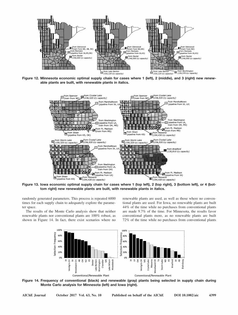
Figures 12 and 13 show the supply chain results for the dif-ferent solution regions for Minnesota and Iowa, respectively.Note that the results for the region where no renewable plantsare built are the base case results; these results were shownpreviously in Figure 8. As keeping transportation at a mini-mum also minimizes the supply chain costs, new renewableplants replace the nearest distribution center as the source forammonia. For example, when comparing the Minnesota sup-ply chains with zero and one new ammonia plant built, notethat the distribution center in Rosemount is no longer used
when the new plant is built. In fact, many of the counties thatwere receiving ammonia from Rosemount when no plants arebuilt instead receive ammonia from the newly built renewableplant in Dexter when ammonia prices are higher and it isselected to be built.
Monte-Carlo analysis
While the carbon tax and ammonia price are importantparameters affecting the optimal supply chain, they are not theonly parameters which have a large impact. In this section, theeffects of four key parameters, which include both the carbontax and ammonia price as well as the electrolyzer scalingexponent and the conversion factor between available windcapacity and renewable plant maximum size, are explored in aMonte Carlo analysis. Such an analysis gives insights on therobustness of the supply chain with respect to different eco-nomic and weather conditions which may be present. In partic-ular, the frequency of building new renewable plants andpurchasing from conventional plants is determined. The distri-butions used for each the four parameters are as follows: first,for the ammonia price, a Gaussian distribution is used basedon the mean and standard deviation from the historical datasince 2008.38 The wind power to maximum plant size conver-sion factor is also varied by a Gaussian distribution with itsmean at the base case value and a standard deviation value of20% of the mean. For carbon tax, an exponential distributionis considered with a mean value at a reasonable $20/t tax, andthe most likely value at the status quo of no carbon tax. Lastly,the electrolyzer capacity exponent varies uniformly from alower bound of 0.67, where the unit scales as well as allothers, to an upper bound of 1, where the unit does not scale atall. For each supply chain, Monte Carlo random samplingusing the given distributions is performed and the optimal sup-ply chain is found by solving the optimization using the
Figure 10. Effect of a carbon tax on annual cost and emissions of economic optimal supply chain for Minnesota(left) and Iowa (right).
Figure 11. Effect of ammonia prices on economic optimal supply chain costs for Minnesota (left) and Iowa (right).
4398 DOI 10.1002/aic Published on behalf of the AIChE October 2017 Vol. 63, No. 10 AIChE Journal
randomly generated parameters. This process is repeated 6000times for each supply chain to adequately explore the parame-ter space.
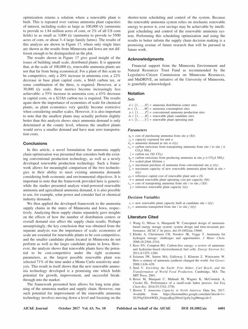
The results of the Monte Carlo analysis show that neitherrenewable plants nor conventional plants are 100% robust, asshown in Figure 14. In fact, there exist scenarios where no
renewable plants are used, as well as those where no conven-tional plants are used. For Iowa, no renewable plants are built44% of the time while no purchases from conventional plantsare made 9.7% of the time. For Minnesota, the results favorconventional plants more, as no renewable plants are built72% of the time while no purchases from conventional plants
Figure 13. Iowa economic optimal supply chain for cases where 1 (top left), 2 (top right), 3 (bottom left), or 4 (bot-tom right) new renewable plants are built, with renewable plants in italics.
Figure 14. Frequency of conventional (black) and renewable (gray) plants being selected in supply chain duringMonte Carlo analysis for Minnesota (left) and Iowa (right).
Figure 12. Minnesota economic optimal supply chain for cases where 1 (left), 2 (middle), and 3 (right) new renew-able plants are built, with renewable plants in italics.
AIChE Journal October 2017 Vol. 63, No. 10 Published on behalf of the AIChE DOI 10.1002/aic 4399

are made only 4.3% of the time. Again, the reason for this is
scale: the largest candidate renewable plant in Iowa, located in
Crystal Lake, is selected the most, 56% of the time. However,
the largest renewable plant in Minnesota, located in Dexter, is
almost 100,000 t/y smaller than the Crystal Lake plant, and as
such is only selected 38% of the time.The observed distributions of costs and emissions are shown
in Figures 15 and 16, respectively. Emissions are plotted on a
log scale since the results vary over orders of magnitude
depending on how many renewable plants are selected. Inter-
estingly, the average cost seen is higher than the base case
cost for the Minnesota supply chain but lower in the Iowa sup-
ply chain. This is likely a result of the Iowa renewable plants
being more competitive than Minnesota renewable plants. As
such, certain parameter values may result in a new renewable
plant being built in Iowa but not in Minnesota, and thus the
relative cost per ton of ammonia will be lower in Iowa but
higher in Minnesota. This explanation is further supported by
the emissions distributions, as Minnesota had a higher likeli-
hood of a high emission supply chain than Iowa.
Analysis of smaller scale systems
The case study results discussed thus far explore which, if
any, renewable plants should be built given certain economic
and demand parameters. The answers that have been obtained,
not surprisingly, say that the largest scale candidate plants are
the most optimal to build since they have lower capital costs
per unit capacity. However, the idea of distributed ammonia
was introduced with the desire to produce this chemical at a
smaller, more distributed scale to take advantage of the geo-
spatially distributed wind supply and agricultural demand. The
framework developed in the article also allows for analysis of
the reverse question; that is, given a specific size of renewable
plant to build, what economic parameters are required to makesuch a plant economically competitive in the supply chain.This analysis allows us to identify policy or technology targetsthat should be met to make smaller scale renewable ammoniaplants economically competitive.
For this analysis, candidate renewable plant capacities wereset to a maximum value of the specific capacity that was beinganalyzed. Three economic parameters were then separatelyanalyzed: the cost of purchasing ammonia from conventionalplants, the cost of a carbon tax, the base case plant capitalcost, and the plant’s capacity exponent. These parameters aregradually increased (in the case of ammonia cost and carbontax), or decreased (in the case of capital cost) until the
Figure 15. Histogram of annual supply chain costs from Monte Carlo analysis for Minnesota (left) and Iowa (right).
Figure 16. Histogram of annual supply chain emissions from Monte Carlo analysis for Minnesota (left) and Iowa(right).
Figure 17. Required changes in parameters for renew-able plants of a certain scale to be econom-ically optimal.
4400 DOI 10.1002/aic Published on behalf of the AIChE October 2017 Vol. 63, No. 10 AIChE Journal
optimization returns a solution where a renewable plant isbuilt. This is repeated over various ammonia plant capacitiesof interest, including scales as large as 100,000 t/y (ammoniato provide to 1.84 million acres of corn, or 2% of all US cornfields) to as small as 3,000 t/y (ammonia to provide to 5500acres of corn, or about 3–4 large family farms). The results ofthis analysis are shown in Figure 17, where only single linesare shown as the results from Minnesota and Iowa are not dif-ferent enough to be distinguished on the plot.
The results shown in Figure 17 give good insight of theissues of building small scale, distributed plants. It is apparentthat, at the scale of 100,000 t/y, renewable ammonia plants arenot that far from being economical. For a plant of this scale tobe competitive, only a 20% increase in ammonia cost, a 22%decrease in base plant capital costs, a $64/t carbon tax, orsome combination of the three, is required. However, at a30,000 t/y scale, these metrics become increasingly lessachievable: a 55% increase in ammonia cost, a 43% decreasein capital costs, or a $218/t carbon tax is required. The resultsagain show the importance of economies of scale for chemicalplants, as plant economics very quickly become restrictivewhen considering smaller scales. However, it is also importantto note that the smallest plants may actually perform slightlybetter than this analysis shows since ammonia demand is onlydetermined at the county level, whereas the smallest plantswould serve a smaller demand and have near zero transporta-tion costs.
Conclusions
In this article, a novel formulation for ammonia supplychain optimization was presented that considers both the exist-ing conventional production technology, as well as a newlydeveloped renewable production technology. Such a frame-work allows for meaningful comparison of the two technolo-gies in their ability to meet existing ammonia demandsconsidering both economic and environmental objectives. It isimportant to note that the framework provided here is generic:while the studies presented analyze wind-powered renewableammonia and agricultural ammonia demand, it is also possibleto use, for example, solar power and consider fuel or chemicalindustry demands.
We then applied the developed framework to the ammoniasupply chains in the states of Minnesota and Iowa, respec-tively. Analyzing these supply chains separately gave insightson the effects of how the number of distribution centers oroverall demand size affect the supply chain results. Perhapsunsurprisingly, the key conclusion that was obtained from theseparate analysis was the importance of scale: economies ofscale are essential for renewable plants to be cost-competitive,and the smaller candidate plants located in Minnesota do notperform as well as the larger candidate plants in Iowa. How-ever, the analysis shows that renewable plants have the poten-tial to be cost-competitive under the right economicparameters, as the largest possible renewable plant wasselected 71% of the time under a Monte Carlo sensitivity anal-ysis. This result in itself shows that the new renewable ammo-nia technology developed is a promising one which holdspotential for growth, improvement, and successful break-through into the market.
The framework presented here allows for long term plan-ning of the ammonia market and supply chain. However, onesuch potential for improvement of the renewable ammoniatechnology involves moving down a level and focusing on the
shorter-term scheduling and control of the system. Because
the renewable ammonia system relies on stochastic renewable
energy to power it, cost savings may be achievable by intelli-
gent scheduling and control of the renewable ammonia sys-
tem. Performing this scheduling optimization and using the
results to better inform the supply chain decision making is a
promising avenue of future research that will be pursued in
future work.
Acknowledgments
Financial support from the Minnesota Environment and
Natural Resources Trust Fund as recommended by the
Legislative-Citizen Commission on Minnesota Resources,
and MnDRIVE, an initiative of the University of Minnesota,
is gratefully acknowledged.
Notation
Sets
d 2 f1; . . . ;Dg = ammonia distribution center sitesm 2 f1; . . . ;Mg = ammonia consumption sitesp 2 f1; . . . ;Pg = conventional ammonia production sitesm 2 f1; . . . ;Rg = renewable plant candidate sitesu 2 f1; . . . ;Ug = renewable plant operating unit
Parameters
ap = cost of purchasing ammonia from site p ($/t)cu = capacity exponent for unit udm = ammonia demand at site m (t/y)�i;j = carbon emissions from transporting ammonia from site i to site j (t
CO2/t NH3)f = carbon tax ($/t CO2)
gp = carbon emissions from producing ammonia at site p (t CO2/t NH3)h = scaled plant lifetime y
np = maximum purchase of ammonia from conventional site p (t/y)nr = maximum capacity of new renewable ammonia plant built at site r
(t/y)qu = reference capital cost of renewable plant unit u ($)r = annual renewable plant operating cost per capacity ($/t)
si;j = cost of transporting ammonia from site i to site j ($/t)v = reference renewable plant capacity (t/y)
Decision Variables
xr = new renewable plant capacity built at candidate site r (t/y)yi;j = ammonia transported from site i to site j (t/y)
Literature Cited
1. Wang G, Mitsos A, Marquardt W. Conceptual design of ammonia-based energy storage system: system design and time-invariant per-formance. AIChE J. In press. doi:10.1002/aic.15660.
2. Klerke A, Christensen CH, Norskov JK, Vegge T. Ammonia forhydrogen storage: challenges and opportunities. J Mater Chem.2008;18:2304–2310.
3. Rees NV, Compton RG. Carbon-free energy: a review of ammonia-and hydrazine-based electrochemical fuel cells. Energy Environ Sci.2011;4:1255–1260.
4. Erisman JW, Sutton MA, Galloway J, Klimont Z, Winiwarter W.How a century of ammonia synthesis changed the world. Nat Geosci.2008;1:636–639.
5. Smil V. Enriching the Earth: Fritz Haber, Carl Bosch, and theTransformation of World Food Production. Cambridge, MA: TheMIT Press, 2001.
6. Reese M, Marquart C, Malmali M, Wagner K, McCormick A,Cussler EL. Performance of a small-scale haber process. Ind EngChem Res. 2016;55:3742–3750.
7. Brown T. Ammonia Capacity in North America. Data Set, 2017.Available from https://fusiontables.google.com/data?docid=1v-XUF9q5X0vbWID_JAzpxaByp28lwlr3gs0y2zg8#map:id=3.
AIChE Journal October 2017 Vol. 63, No. 10 Published on behalf of the AIChE DOI 10.1002/aic 4401

8. United States Department of Agriculture. National Agriculture Sta-tistics Service. Corn: Planted Acreage by County, (Map). 2015.Available from https://www.nass.usda.gov/Charts_and_Maps/graphics/CR-PL-RGBChor.pdf.
9. National Renewable Energy Laboratory. United States - AnnualAverage Wind Speed at 80 m. (Map). 2011. Available from https://apps2.eere.energy.gov/wind/windexchange/pdfs/wind_maps/us_wind-map_80meters.pdf.
10. Chopra S, Meindl P. Supply Chain Management: Strategy, Planning,and Operation, 6th ed. Essex, UK: Pearson Education Limited,2016.
11. Tester JW, Drake EM, Driscoll MJ, Golay MW, Peters WA. Sustain-able Energy: Choosing among Options, 2nd ed. Cambridge, MA:The MIT Press, 2012.
12. Cambero C, Sowlati T. Assessment and optimization of forest bio-mass supply chains from economic, social, and environmental per-spectives - a review of literature. Renew Sustainable Energy Rev.2014;36:62–73.
13. Kim J, Realff MJ, Lee JH. Optimal design and global sensitivityanalysis of biomass supply chain networks for biofuels under uncer-tainty. Comput Chem Eng. 2011;35:1737–1751.
14. Marvin WA, Schmidt LD, Benjaafar S, Tiffany DG, Daoutidis P.Economic optimization of a lignocellulosic biomass-to-ethanol sup-ply chain. Chem Eng Sci. 2012;67:68–79.
15. Marvin WA, Schmidt LD, Daoutidis P. Biorefinery location andtechnology selection through supply chain optimization. Ind EngChem Res. 2013;52:3192–3208.
16. Kelloway A, Marvin WA, Schmidt LD, Daoutidis P. Process designand supply chain optimization of supercritical biodiesel synthesisfrom waste cooking oils. Chem Eng Res Design. 2013;91:1456–1466.
17. You F, Tao L, Graziano DJ, Snyder SW. Optimal design of sustain-able cellulosic biofuel supply chains: multiobjective optimizationcoupled with life cycle assessment and input-output analysis. AIChEJ. 2012;58:1157–1180.
18. Yue D, Slivinsky M, Sumpter J, You F. Sustainable design and oper-ation of cellulosic bioelectricity supply chain networks with lifecycle economic, environmental, and social optimiation. Ind EngChem Res. 2014;53:4008–4029.
19. Tong K, Gleeson MJ, Rong G, You F. Optimal design of advanceddrop-in hydrocarbon biofuel supply chain integrating with existingpetroleum refineries under uncertainty. Biomass Bioenergy. 2014;60:108–120.
20. Guillen-Gosalbez G, Mele FD, Grossman IE. A bi-criterion optimi-zation approach for the design and planning of hydrogen supplychains for vehicle use. AIChE J. 2010;56:650–667.
21. Mele FD, Kostin AM, Guillen-Gosalbez G, Jimenez L. Multiobjec-tive model for more sustainable supply chains. A case study of thesugar cane industry in Argentina. Ind Eng Chem Res. 2011;50:4939–4958.
22. Hasan MMF, Boukouvala F, First EL, Floudas CA. Nationwide,regional, and statewide CO2 capture, utilization, and sequestrationsupply chain network optimization. Ind Eng Chem Res. 2014;53:7489–7506.
23. Miura D, Tezuka T. A comparitive study of ammonia energy sys-tems as a future energy carrier, with particular reference to vehicleuse in Japan. Energy. 2014;68:428–436.
24. Schulz E, Diaz M, Bandoni J. Supply chain optimization of large-scale continuous processes. Comput Chem Eng. 2005;29:1305–1316.
25. UNIDO, IFDC, editors. Fertilizer Manual. Norwell, MA: KluwerAcademic Publishers, 1998.
26. Dutta S. Optimization in Chemical Engineering. Delhi, India: Cam-bridge University Press, 2016.
27. Tawarmalani M, Sahinidis NV. A polyhedral branch-and-cutapproach to global optimization. Mathematical Programming. 2005;103(2):225–249.
28. Minnesota Department of Agriculture. 2012 Minnesota AgriculturalStatistics, Technical Report, 2013. Available from https://www.leg.state.mn.us/docs/2012/other/121196.pdf.
29. Thessen G, Adamson C, Harwig D. Iowa Agricultural Statistics.Technical Report, 2016. Available from https://www.nass.usda.gov/Statistics_by_State/Iowa/Publications/Annual_Statistical_Bulletin/2015/IA%20Bulletin%202015.pdf.
30. United States Department of Agriculture. US Plant Nutrient Use byCorn, Soybeans, Cotton, and Wheat, 1964–2012, Data Set, 2013.Available from https://www.ers.usda.gov/data-products/fertilizer-use-and-price/.
31. Schnitkey G. Nitrogen fertilizer prices and 2015 planting decitions.Farmdoc Daily. 2014;4:195.
32. Wood S, Cowie A. A Review of Greenhouse Gas Emission Factorsfor Fertilizer Production. Research and Development Division, StateForests of New South Wales, 2004.
33. United States Department of Labor. Heavy and Tractor-TrailerTruck Drivers, Data Set, 2015.
34. Google, Inc. Google Maps Distance Matrix API, 2017.35. United States Energy Information Administration. How much Carbon
Dioxide is Produced per Kilowatthour when Generating Electricityfrom Fossil Fuels? Data Set, 2016. Available from https://www.eia.gov/tools/faqs/faq.php?id=74&t=11.
36. OpenEI. Map of Wind Farms, Data Set, 2017. Available from http://en.openei.org/wiki/Map_of_Wind_Farms.
37. National Renewable Energy Laboratory. Current (2009) state-of-the-art hydrogen production cost estimate using water electrolysis. Tech-nical Report, 2009. Available from https://www.hydrogen.energy.gov/pdfs/46676.pdf.
38. Schnitkey G. Current fertilizer prices and projected 2016 fertilizercosts. Farmdoc Daily. 2015;5:232.
Manuscript received Feb. 10, 2017, and revision received June 9, 2017.
4402 DOI 10.1002/aic Published on behalf of the AIChE October 2017 Vol. 63, No. 10 AIChE Journal