A Fractal Comparison of M.C. Escher’s and H. von Koch’s ... taking the basic shapes that Escher...
19
A Fractal Comparison of M.C. Escher’s and H. von Koch’s Tessellations B. Van Dusen 1 , B.C. Scannell 2 and R.P. Taylor 2 1 School of Education, University of Colorado, Boulder, 80309, USA 2 Physics Department, University of Oregon, Eugene, OR 97403, USA Abstract: M.C. Escher’s tessellations have captured the imaginations of both artists and mathematicians. Circle Limit III is the most intricate of his tessellations, featuring patterns that repeat at increasingly fine scales. Although his patterns follow a scaling law determined by hyperbolic geometry, his work is often mistakenly described as following fractal geometry. Here, we perform a ‘box-counting’ scaling analysis on Circle Limit III and an equivalent mono- fractal pattern based on a Koch Snowflake. Whereas our analysis highlights the expected visual differences between Escher’s hyperbolic patterns and the simple mono-fractal, the analysis also identifies unexpected similarities between Escher’s work and the bi-fractal poured paintings of Jackson Pollock. Keywords: Escher, Fractal, hyperbolic space, art, and computer analysis Published: Published: Fractals Research, 116, ISBN 9780979187469 (2012)
-
Upload
nguyenkhanh -
Category
Documents
-
view
216 -
download
0
Transcript of A Fractal Comparison of M.C. Escher’s and H. von Koch’s ... taking the basic shapes that Escher...

A Fractal Comparison of M.C. Escher’s and H. von Koch’s
Tessellations
B. Van Dusen1, B.C. Scannell2 and R.P. Taylor2
1School of Education, University of Colorado, Boulder, 80309, USA
2Physics Department, University of Oregon, Eugene, OR 97403, USA
Abstract: M.C. Escher’s tessellations have captured the imaginations of both
artists and mathematicians. Circle Limit III is the most intricate of his
tessellations, featuring patterns that repeat at increasingly fine scales. Although
his patterns follow a scaling law determined by hyperbolic geometry, his work
is often mistakenly described as following fractal geometry. Here, we perform a
‘box-counting’ scaling analysis on Circle Limit III and an equivalent mono-
fractal pattern based on a Koch Snowflake. Whereas our analysis highlights the
expected visual differences between Escher’s hyperbolic patterns and the simple
mono-fractal, the analysis also identifies unexpected similarities between
Escher’s work and the bi-fractal poured paintings of Jackson Pollock.
Keywords: Escher, Fractal, hyperbolic space, art, and computer analysis
Published: Published: Fractals Research, 1-‐16, ISBN 978-‐0-‐9791874-‐6-‐9 (2012)
1.1 Introduction
It has become popular to view the spectrum of disciplines as a circle, with
mathematics and art lying so far apart that they become neighbors. Two artists are
celebrated as proof of this theory - Leonardo da Vinci (1452-1519) and Maurits Escher
(1898-1972). Da Vinci combined mathematics and art to search for the possible, resulting
in functional designs such as his famous flying machines. In contrast, Escher searched for
the impossible. As we will see, he created images by distorting nature’s rules.
In this article, we focus on Escher’s prints of tessellations [1], of which the
woodcut Circle Limit III (1958) is the most intricate. Inspired by the Islamic tiles that he
saw during a trip to the Alhambra in Spain, Escher took the bold step of incorporating
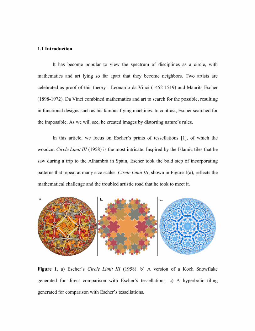
patterns that repeat at many size scales. Circle Limit III, shown in Figure 1(a), reflects the
mathematical challenge and the troubled artistic road that he took to meet it.
Figure 1. a) Escher’s Circle Limit III (1958). b) A version of a Koch Snowflake
generated for direct comparison with Escher’s tessellations. c) A hyperbolic tiling
generated for comparison with Escher’s tessellations.

To achieve the desired visual balance, he insisted that the shrinking patterns
converge towards a circular boundary. In Escher’s words, the repeating patterns emerge
from the circular boundary “like rockets”, flowing along curved trajectories until they
“lose themselves” once again at the boundary [2]. Making his patterns fit together
required considerable thought and a helping hand from mathematics. After several flawed
attempts, Escher finally found the solution in an article written several years earlier by
the British geometer H.S.M. Coxeter [3, 4].
These flowing patterns have captured the imaginations of both artists and
mathematicians for over half a century. Yet along the way, their connection with nature
has fallen by the way side. His work is often presented as an elegant solution to a purely
academic exercise of mathematics - a clever visual game. In fact, Escher’s interest lay in
the fundamental properties of patterns that appear in the real world. He declared: “We are
not playing a game of imaginings – we are conscious of living in a material three
dimensional reality.” [2].
Escher’s artistic interest in the physical world is emphasized by the sketches of
trees that he completed in the same era as Circle Limit III [1]. These sketches
demonstrate how branch patterns repeat at different size scales and how they become
distorted when reflected in the rippled surface of a pond. Given his quest for distortion, it
would be surprising to find that Circle Limit III was an exact replication of nature’s
patterns. In this article, we focus on the fact that his patterns shrink at a different rate than
those found in nature. The artist used the hyperbolic geometry described in Coxeter’s
article [3, 4], rather than the fractal geometry that describes natural patterns [5].

To highlight the visual differences between Escher’s hyperbolic geometry and
fractal geometry, we will apply a computer scaling analysis to Circle Limit III and an
equally famous pattern from fractal geometry – the Koch Snowflake. The Koch curve
was created fifty years earlier by the mathematician Niels Fabian Helge von Koch (1870-
1924). Koch’s curve consisted of triangles that repeat at increasingly fine scales, so
building up the edge of a snowflake [6].
To facilitate a direct comparison with Escher’s patterns, we created the snowflake
pattern shown in Figure 1(b) and the hyperbolic tiling of clouds shown in Figure 1(c).
Whereas the snowflake pattern features interlocking tessellations similar to Circle Limit
III, the scaling properties of these tessellations are set by the triangles of the central
snowflake, which are fractal rather than hyperbolic. The cloud pattern was created using
commercially available software and shows an exact hyperbolic pattern. By examining
the results of the scaling analysis, we discuss the visual implications of Escher’s
deviations from the fractal and hyperbolic scaling of nature’s shapes.
We note that significant formal mathematical comparisons between fractal and
hyperbolic geometries have been made previously, notably by Stratmann [7]. Here we
use a different analytical technique, by comparing the edge patterns of the three art works
of Figure 1 employing a traditional fractal analysis called the “box counting” technique.
This technique is particularly appropriate because visual perception studies highlight the
importance of edges for distinguishing patterns [8]. Furthermore, the box-counting
method assesses the space-filling characteristics of these edges at different size scales.
Space-filling properties have been found to be an important aesthetic quality for other
forms of abstract art featuring multi-scale patterns, most notably the poured paintings of

American artist Jackson Pollock (1912-1956) [9]. Whereas our analysis highlights the
expected visual differences between Escher’s hyperbolic patterns and the simple Koch
fractal, the analysis also identifies unexpected visual similarities between Escher’s work
and the fractal poured paintings of Pollock.
1.2 Escher’s Construction of Multi-scale Tessellations
Tessellations are patterns that fill the surface of a plane without any overlaps or
gaps. Most tessellation designs in art feature component tiles which are identical in size.
In the four piece series Circle Limit, Escher instead created tessellations that appear to be
‘going to infinity’ as they approach the edge of a circle: in other words, their size
diminishes towards the infinitesimally small as the edge is approached. To create this
visual effect, he had to generate tile shapes that are not typically tiled together.
When taking the basic shapes that Escher used in his Circle Limit pieces and tiling
them together they don’t create a flat surface. Instead of fitting together evenly in two
dimensions, the pieces form the hyperbolic geometry shown in Figure 2. A hyperbolic
geometry looks much like a saddle: on one axis, the surface rises upward from the origin
(symbolized by the dot) and on the other axis the surface drops downward. When this
hyperbolic surface is viewed directly from above, it appears to spread out indefinitely and
any tiles ‘drawn’ on the surface become more distorted the further they get from the
origin. Thus, although all the tiles have equal size on the hyperbolic surface, they appear
to shrink towards the edge when viewed this way.

Figure 2. Hyperbolic geometries form the shape of a saddle with the surface
rising along one axis and dropping along the other axis.
To make the entire surface viewable, Escher translated the surface onto a Poincaré
disk [10]. A Poincaré disk is a circle that represents an infinite region of space. As the
circular edge is approached, the images diminish at such a rate that they appear to be
getting both infinitely smaller and closer to the circle’s edge, without ever actually
reaching it. By using this Poincaré disk model, Escher was able to give the impression of
an infinite array of tile images within a limited space, and unlike other disk models; the
shape of the tiles stays recognizable as they approach the circular boundary.
In his first attempt at using the Poincaré disk model, Escher was dissatisfied with
his final product, Circle Limit I (1958). He felt that it lacked “traffic flow” and unity of
color in each row [1]. Escher was much happier with what is referred to as his most
accomplished Circle Limit piece, Circle Limit III:
“Circle Limit I, being a first attempt, displays all sorts of shortcomings...
There is no continuity, no “traffic flow,” nor unity of colour in each row...
In the coloured woodcut Circle Limit III, the shortcomings of Circle Limit
I are largely eliminated. We now have none but “through traffic” series,
and all the fish belonging to one series have the same colour and swim
after each other head to tail along a circular route from edge to edge...
Four colours are needed so that each row can be in complete contrast to its
surroundings.” [1]
In Circle Limit III, Escher tessellates four different colored fish. Each fish has one
of its fins touching the fins of three fish and its other fin touching the fins of two fish.
Each fish nose touches two other fishes’ noses and three tails. As shown in Figures 3(a)
and 3(b), this pattern is a tessellation of octagons. Each octagon is met at its corner with
two other octagons.


Figure 3. a) Escher’s octagonal pattern used in Circle Limit III. b) The octagonal pattern
overlaying the circular arcs created by the fishes’ spines, color-coded to each type of fish.
c) The octagonal pattern laid over Circle Limit III.
When a hyperbolic tessellation is mapped onto a Poincaré disk, straight lines
become circular arcs that are orthogonal to the bounding circle. This is demonstrated with
the ‘flow lines’ shown in Figure 3(b). In a mistake that appears to be unbeknownst to
Escher himself, unlike his other Circle Limit pieces, Circle Limit III’s arcs aren’t true
hyperbolic arcs. When analyzed by Coxeter, the white circular arcs approach the
boundary of the disk at 80°, not the 90° of hyperbolic line [4]. Despite this minor
aberration in the pattern, it still gives a viewer the strong sense of the pattern approaching
the infinite. Further details of Escher’s hyperbolic design can be found elsewhere [11].
1.3 Fractal Analysis of Circle Limit III
The tessellations within Escher’s Circle Limit series are often mistaken for fractal
images. Like fractals, the Circle Limit series have self-similar patterns that recur at
increasingly finer scales. However, Escher’s tessellations decrease at a hyperbolic-like
rate, rather than the power law rate at which fractals decrease [5, 9, 12]. The visual
difference of these three scaling rates is highlighted in Figure 4, where the edge patterns
for the three tessellations designs have been isolated.

Figure 4. The edge patterns of a) the Koch Snowflake, b) Circle Limit III, and c) a true
hyperbolic tiling.
This isolation of the edge patterns also allows their scaling behavior to be
analyzed using the “box counting” technique [9, 12]. Adopting this technique, the image
of white edges is covered with a computer-generated grid of identical squares (or
“boxes”), as shown in Figure 5. By analyzing which of the squares are “occupied” (i.e.,
contains a part of the white edge pattern) and which are “empty” (shaded blue in Figure
5), the statistical qualities of the edge pattern can be calculated.

Figure 5. A section of Circle Limit III overlaid with a grid of boxes. Boxes containing
white pixels are counted in the box counting procedure. This count is repeated for
increasingly fine boxes sizes (a, b, c).
Reducing the square size in the grid is equivalent to looking at the pattern at a
finer magnification. Thus, in this way, the pattern’s statistical qualities can be compared
at different magnifications. Specifically, if N, the number of occupied squares, is counted
as a function of L, the width of each square, then for fractal behavior N(L) scales
according to the power law relationship N(L) ~ L-D [5, 9, 12]. The exponent D is called
the fractal dimension and its value can be extracted from the gradient of the “scaling plot”
of log(N) plotted against log(1/L).
The scaling plots generated by the box-counting technique are shown in Figure 6.
The analysis is performed over a magnification range lying between coarse and fine scale
cut-offs. The coarse scale cut-off is set by the box size (L ~ 6cm) at which the grid has
less than 50 boxes: at larger L values, there are insufficient boxes to ensure reliable
counting statistics [9]. The fine scale cut-off is set by the box size (L ~ 0.5mm)
corresponding to approximately 3 pixels of the image: at smaller box sizes, the count is
compromised by the resolution limit of the image. Between these two cut-offs, the
scaling plot for the Koch Snowflake displays the straight power-law line expected for a
fractal pattern. In contrast, the data for Circle Limit III fails to condense onto a straight
line. To interpret the visual significance of this curved line, we need to consider the
importance of the fractal’s power law line in more detail.

Figure 6. Scaling plots obtained from the box counting analysis of the Koch Snowflake
(blue data), Circle Limit III (red data), and a true hyperbolic tiling (green data). The
analyzed images had dimensions 42 cm by 42 cm and resolution of 63 pixels per cm.
The power law line generates the scale-invariant properties that are central to
fractal geometry. It also quantifies the crucial role played by D in determining the
pattern’s visual appearance. D corresponds to the gradient of the scaling plot. Therefore,
a high D value is a signature of a large N value at small L and reflects the fact that many
small boxes are being filled by fine structure. This can be seen, for example, for the set of
Koch curves shown in Figure 7. The fine features play a more dominant ‘space coverage’
role for the high D pattern than for the low D pattern. For fractals described by a low D

value, the patterns observed at different magnifications repeat in a way that builds a
relatively smooth-looking shape compared to the complex, detailed structure of high D
patterns.


Figure 7. Koch curves with D values ranging from 1.1 (top) to 1.9 (bottom).
Perception experiments confirm that raising the D value of the fractal pattern
increases its perceived roughness and complexity [13, 14, 15]. Clearly, D is a highly
appropriate tool for quantifying fractal complexity. Traditional measures of visual
patterns quantify complexity in terms of the ratio of fine structure to course structure. D
goes further by quantifying the relative contributions of the fractal structure at all the
intermediate magnifications between the course and fine scales.
As expected from the previous formal comparisons of hyperbolic and fractal
geometry [7], Escher’s tessellations deviate from the straight data line of fractal geometry.
The importance of Figure 6 lies in the fact that it highlights the precise deviation in terms
of the space-coverage of the pattern at different scales. How, then, do we interpret the
visual impact quantified by the curved data line for Circle Limit III? Because of its
curvature, the data line can’t be quantified by a D value. Nevertheless, the steepness of
the line holds the same visual consequences as for a fractal pattern: steeper gradients
indicate that the space-coverage of the pattern is changing at a faster rate when zooming
into finer size scales. Intriguingly, the rate characterizing Circle Limit III can be seen to
‘weave’ around the constant rate set by the fractal geometry of the Koch pattern. More
precisely, the rate is steeper than the Koch fractal at coarse scales but then shallower at
the finer scales. A visual inspection of Figures 1 and 4 confirms that this is indeed the
case.
As noted previously, Figure 6 shows that Escher’s work doesn’t create a constant
line that is attributed to fractals. However, it is also worth noting that Escher’s curve
deviates from a true hyperbolic geometry. Our box counting program is able to show that
true hyperbolic geometries have a slight curve in their data, while Escher’s data has a
more significant deviation from a straight line.
1.4 Conclusions
In contrast to the traditional view of Escher’s achievements in terms of abstract
mathematics, in this article we have instead concentrated on his interest in nature’s
patterns. To do this, we presented a comparison of Escher’s repeating tessellations and
those of fractal geometry, and so showed that his patterns deviated from nature’s rules of
scaling as well as those of hyperbolic geometry.
Intriguingly, Circle Limit III was created many years before B.B. Mandelbrot’s
“Fractal Geometry of Nature” made nature’s scaling properties well known [5]. Therefore,
the intriguing question raised in this article is the extent to which Escher knew about the
distortions of nature that he captured so precisely in much of his art. Our results indicate
that Escher knew of the mild distortion from fractals that hyperbolic tiling produced, but
that he chose to perform a modified hyperbolic tiling to produce an even larger distortion.
A common theme that emerges from fractal studies is that artists were mimicking
nature’s fractals prior to their scientific discovery. Perhaps this is a consequence of the
intimacy resulting from art and mathematics being so far away and yet so close. Escher’s
own words hint at knowledge of his distortions of nature: “The reality around us… is too
common, too dull, too ordinary for us. We hanker after the unnatural or supernatural, that
which does not exist, a miracle” [1]. Perhaps he achieved this miracle in what he referred
to as the “deep, deep infinity” of his repeating patterns.
What, though, are the aesthetic implications of Escher’s deviations from fractal
geometry? Does the fact that Circle Limit III diminishes at a varying rate similar to the
curvature of the hyperbolic surface hold important potential for visual perception studies?
Previous perception experiments have concentrated on patterns generated by the constant
scaling rate of simple fractals [16, 17, 18] and so a detailed quantification of the aesthetic
impact of the curved rate will have to await future experiments. Nevertheless, an initial
observation can be made by comparing Circle Limit III to the poured paintings of Jackson
Pollock. Although Pollock’s paintings are fractal, and are therefore described by a
fundamentally different geometry to Escher’s hyperbolic patterns, the two art works have
an unexpected shared scaling characteristic, as follows. Pollock’s paintings have been
shown to be ‘bi-fractal’ – patterns at the large size scales created by his body motions are
quantified by a high D value, while the splatter patterns observed at finer scales have a
low D value [9]. The visual consequence of this bi-fractal behavior is similar to that of
the hyperbolic curve of Escher’s work – a steep rate of space-coverage at large scales
followed by a shallow rate at finer scales. Although we emphasize the preliminary
character of this observation, it is nevertheless intriguing to hypothesize that both artists
regarded the constant scaling rate of ‘mono’ (single D) fractals, such as the Koch
snowflake, to be too monotonous to exhibit aesthetic appeal.
1.5 References
[1] M.C. Escher, Escher on Escher, Abrams, New York (1989).

[2] B. Ernst, The Magic Mirror of M.C. Escher, Benedikt Taschen Verlag, Cologne,
Germany (1995).
[3] H.S.M. Coxeter, "The Non-Euclidean Symmetry of Escher's Picture 'Circle Limit III'".
Leonardo, 12, 19-25 (1979).
[4] H.S.M. Coxeter. The trigonometry of Escher’s woodcut ”Circle Limit III”,
Mathematical Intelligencer, 18 42–46 (1996). This his been reprinted by the
American Mathematical Society in M.C. Escher’ s Legacy: A Centennial Celebration,
D. Schattschneider and M. Emmer editors, Springer Verlag, New York, 297–304
(2003).
[5] B.B. Mandelbrot, The Fractal Geometry of Nature, Freeman, New York (1982).
[6] H. von Koch, "On a continuous curve without tangents, constructible from elementary
geometry" (1904).
[7] B. O. Stratmann, “Fractal geometry on hyperbolic manifolds”, in Non–Euclidean
Geometries; Janos Bolyai Memorial Volume, Eds.: A. Prekopa, E. Molnar, Springer
Verlag (2005) 227–249.
[8] B.E. Rogowitz & R.F. Voss, Shape perception and low dimensional fractal boundary
contours. Proceedings of the conference on human vision: Methods, Models and
Applications, S.P.I.E., 1249, 387-394, (1990).
[9] R.P. Taylor, R. Guzman, T.M. Martin, G. Hall, A.P. Micolich, D. Jonas, B.C.
Scannell, M.S. Fairbanks, & C.A. Marlow, Authenticating Pollock paintings with
fractal geometry, Pattern Recognition Letters, 28, 695, (2007).

[10] J.W. Anderson, “Hyperbolic Geometry”, Springer Undergraduate Mathematics
Series. Springer-Verlag London Ltd., London, second edition, (2005).
[11] D. Durham, “The Family of Circle Limit III Escher Patterns”,
http://citeseerx.ist.psu.edu/viewdoc/download?doi=10.1.1.132.2674&rep=rep1&t
ype=pdf
[12] R.P. Taylor and J.C. Sprott, “Biophilic Fractals and the Visual Journey of Organic
Screen-savers”, Non-Linear Dynamics, Psychology, and the Life Sciences, 12
117-129 (2008).
[13] J.E. Cutting and J.J. Garvin, “Fractal Curves and Complexity”, Perception and
Psychophysics, 42 365-370 (1987).
[14] D.L. Gilden, M.A. Schmuckler and K. Clayton, “The Perception of Natural
Contour”, Psychological Review, 100 460-478 (1993).
[15] A.P. Pentland, “Fractal-based Description of Natural Scenes”, IEEE Pattern
Analysis and Machine Intelligence, PAMI-6, 661-674 (1984).
[16] D. Aks and J.C. Sprott “Quantifying Aesthetic Preference for Chaotic Patterns”,
Empirical Studies of the Arts, 14 1-16 (1996).
[17] B. Spehar, C. Clifford, B. Newell and R.P. Taylor, “Universal Aesthetic of Fractals.
Chaos and Graphics, 37, 813-820 (2003).
[18] R.P. Taylor, “Reduction of Physiological Stress using Fractal Art and Architecture”,
Leonardo, 39 245-250 (2006).


![The Symmetry of “Circle Limit IV” and Related Patternsddunham/bridges09.pdf · indentation of Escher’s original) are available from the M.C. Escher web site [4]. So Escher’s](https://static.fdocuments.in/doc/165x107/5c110fdf09d3f25a2c8b7e61/the-symmetry-of-circle-limit-iv-and-related-patterns-ddunham-indentation.jpg)