A formalism to describe concurrent non-deterministicsystems and an application of it by analysing systems fordanger of deadlockHuis in 't Veld, R.J.

Published: 01/01/1988

Document VersionPublisher’s PDF, also known as Version of Record (includes final page, issue and volume numbers)

Please check the document version of this publication:

• A submitted manuscript is the author's version of the article upon submission and before peer-review. There can be important differencesbetween the submitted version and the official published version of record. People interested in the research are advised to contact theauthor for the final version of the publication, or visit the DOI to the publisher's website.• The final author version and the galley proof are versions of the publication after peer review.• The final published version features the final layout of the paper including the volume, issue and page numbers.

Link to publication

Citation for published version (APA):Huis In T Veld, R. J. (1988). A formalism to describe concurrent non-deterministic systems and an application ofit by analysing systems for danger of deadlock. (EUT report. E, Fac. of Electrical Engineering; Vol. 88-E-200).Eindhoven: Technische Universiteit Eindhoven.

General rightsCopyright and moral rights for the publications made accessible in the public portal are retained by the authors and/or other copyright ownersand it is a condition of accessing publications that users recognise and abide by the legal requirements associated with these rights.

• Users may download and print one copy of any publication from the public portal for the purpose of private study or research. • You may not further distribute the material or use it for any profit-making activity or commercial gain • You may freely distribute the URL identifying the publication in the public portal ?

Take down policyIf you believe that this document breaches copyright please contact us providing details, and we will remove access to the work immediatelyand investigate your claim.

Download date: 17. Jun. 2018

A Formalism to Describe Concurrent Non-Deterministic Systems and an Application of it by Analysing Systems for Danger of Deadlock by R.J. Huis in 't Veld

EUT Report 88-E-200 ISBN 90-6144-200-1

August 1988

ISSN 0167- 9706

Eindhoven University of Technology Research Reports

EINDHOVEN UNIVERSITY OF TECHNOLOGY

Faculty of Electrical Engineering

Eindhoven The Netherlands

Coden: TEUEDE

A FORMALISM TO DESCRIBE CONCURRENT NON-DETERMINISTIC SYSTEMS

AND

AN APPLICATION OF IT BY ANALYSING SYSTEMS FOR DANGER OF DEADLOCK

by

R.J. Huis in 't Veld

EUT Report 88-E-200

ISBN 90-6144-200-1

Eindhoven

August 1988

CIP-GEGEVENS KONINKLIJKE BIBLIOTHEEK, DEN HAAG

Huis in 't Veld, R.J.

A formalism to describe concurrent non-deterministic systems and an application of it by analysing systems for danger of deadlock / by R.J. Huis in It Veld. -Eindhoven: University of Technology, Faculty of Electrical Engineering. - Fig. - (EUT report, 155N 0167-9708, 88-E-200) Met lit. opg., reg. ISBN 90-6144-200-1 5150 520.6 UDC 510.5 NUGI 811 Trefw.: procesalgebra.

A FORMALISM TO DESCRIBE CONCURRENT NON-DETERMINISTIC SYSTEMS

AND

AN APPLICATION OF IT BY ANALYSING SYSTEMS FOR DANGER OF DEADLOCK

R.J. Huis in 't Veld Faculty of Electrical Engineering,' Digital Systems Group (EB)

Eindhoven University of Technology P.O. Box 513, 5600 MB Eindhoven, The Netherlands

Abstract: A formalism is introduced to describe the behaviour of systems built out of concurrently running mechanisms. The central notion in this formalism is called process. It is used to specify the behaviour of these systems. Furthermore, criteria to differentiate between specifications are discussed. Each of these criteria will be formalized by an equivalence relation on processes. Finally, the formalism is used to analyse the behaviour of systems for deadlock-like properties. Several concepts describing these properties are introduced. It appears that a system may show one of these properties, while its components do not. For this purpose, theorems are derived. They state the conditions under which larger systems may be built out of smaller ones, without introducing deadlock-like properties.

- iii -

CONTENTS

Preface 1

1. The Formalism

1.0 Introduction 3 1.1 Process 3 1.2 Concurrency 8 1.3 Equivalence relations on processes 10 1.4 Properties of Bisimulation Equivalence 19

2. Deadlock

2.0 Introduction 23 2.1 Locked and Lockfree 25 2.2 Construction of lockfree systems 29 2.3 A substitution property 32 2.4 Deadlockfree 37

3. Other Concepts

3.0 Introduction 39 3.1 Disablefree 39 3.2 Ignorefree 40

4. Conclusions 42

5. References 43

- iv -

PREFACE

CCS (a Calculus of Communicating Systems) [6], CSP (Communicating Sequential

Processes) [3] and Trace Theory [5] have been evolved to formalize the

reasoning about systems built out of concurrently running mechanisms. Each of

these formalisms shows how abstract specifications of the behaviour of a

system and its components may be given. Then, properties of a system may be

expressed by predicates over these specifications.

In this report. we combine the mayor features of CCS and Trace Theory into a

new formalism. The central notion in this formalism is called process. It is

used to specify the behaviour of systems bull t out of concurrently running

mechanisms. Also, criteria to differentiate between the behaviour of these

systems are discussed. Each of these criteria is formalized by an equivalence

relation on processes. Furthermore, we apply the formalism to analyse systems

for danger of deadlock. A concept in terms of our formalism is presented that

corresponds to our intuitive meaning of deadlock. It appears that a system

may have danger of deadlock while its components do not. For this purpose, a

theorem is derived. It states the conditions under which larger deadlockfree

systems may be built out of smaller ones. Finally, we treat other, to

deadlock related propertles of systems.

We conclude this preface with some notational conventions used throughout

this report. Slightly unconventional notations are used for variable binding

constructs. Universal quantification is denoted by (81: d: E) where B is the

quantifier, 1 is a list of bound variables, d delineates the range of each of

these variables, and E is the quantified expression. Similarly, (E 1: d: E)

denotes existential quantification. Furthermore, we use in the same way the

quantifiers !..! and 0 to denote continued unification and continued

intersection respectively.

Given two sets X and Z. The proof that X is a subset of Z (X ~ Z) may run

like: X ~ Y and Y ~ Z for some set Y. Henceforth, we record such proofs as

follows:

- 1 -

x ~ { hint why X ~ Y }

Y ~ { hint why Y ~ Z }

Z

- 2 -

1. THE FORMALISM

1. 0 Introduction

The behaviour of a system built out of concurrently running mechanisms may

show some unwanted aspects. To determine whether these aspects are present in

the behaviour of a system, a formalism is used that is based upon CCS and

Trace Theory. In this chapter the formalism is presented.

We start by introducing the notion process. At first, a process is used to

describe the behaviour of a mechanism. Later on, this is generalized to

describe the behaviour of a system built out of concurrently running

mechanisms. Then, we continue by discussing criteria to differentiate between

the behaviour of systems. Each of these criteria is formalized by an

equivalence relation on the universe of processes. Finally, some properties

are derived for the strongest of these relations.

1.1 Process

We postulate two disjoint infinite sets Id and II. The elements of Id are

called behaviour-names. Elements and subsets of 1\ are called action-symbols

and alphabets respectively.

Let A be a set. The set of all finite-length sequences of elements of A is

denoted by A*. The empty sequence is denoted by c. Elements of 11* are called

traces.

Small and large letters near the beginning of the Latin alphabet are used to

denote action-symbols and alphabets respectively, and small and large letters

near the end of the Latin alphabet are used to denote traces and

behaviour-names respectively.

Furthermore, we denote by Exp the set of expressions defined by the following

syntax in Backus-Naur Form:

- 3 -

E .. = a:E

E + E

X

NIL

- 4 -

where a and X range over A and Id respectively. NIL is a special symbol that

is not an element of A or Id. Additionally, we assume that for expressions

Ei, i" 0, the infinite sequence EO + E1 + E2 + ... (abbreviated by

(+i:i .. O:Ei» is also an expression.

A transition-function is a partial function from Id to Exp. Frequently, we

write a transition-function 'Y as a set of pairs {(X,'Y(XllIXe dom('Y)}. For

transition-functions 'YO and 'Y1 with disjoint domains, we denote by 'YO u 'Y1

the transition-function that corresponds to the union of the with 'YO and 'Y1

associated sets of pairs.

We now have a sufficient base to introduce the notion process. Assume E to be

an expression, A to be an alphabet and 'Y to be a transition-function. We call

the triple <E,A,'Y> a process if and only if the elements of A are the only

action-symbols that occur in E and in the expressions in the range of 'Y. To

refer more easily to the three components that make up a process P,

P = <E,A,'Y>, we denote by rP the expression E, by ~P the alphabet A and by uP

the transition-function 'Y.

We attach an operational semantics to processes, by defining for each

action-symbol a the binary relation ~ on the universe P of processes.

Definition 1.1.0

For each action-symbol a, we denote by ~ the smallest binary relation on P

satisfying:

i) (a:E,A,'Y) ~ (E,A,'Y)

ii) if (EO,A,'Y) ~ (E,A,'Y) or (E1,A,'Y) ~ (E,A,':!)

then (EO + E1,A,'Yl ~ (E,A,'Yl

iii) if ('Y(X),A,':!) ~ (E,A,'Y) then (X,A,':!) ~ (E,A,'Y)

where E, EO and E1 are expressions, A is an alphabet, X is a behaviour-name,

and 'Y is a transition-function.

(End of Definition)

We continue by extending the binary relations on the universe of processes

from action-symbols to traces.

- 5 -

Definition 1. 1. 1 t For a trace t, we recursively define the binary relation --7 on P as follows

i) P ---E... P

ii) For trace s and action-symbol a:

PO ~ P2 = (EP1:P1 e P:PO ~ P1 A P1 ~ P2)

(End of Definition)

The operational semantics we have attached to a process P may be expressed

graphically. The binary relations a --7 , a eA. and the set Q,

Q = {P' I (Es: s e ~p·:P ~ P' )}, specify a rooted, directed, connected graph.

This graph is called the state graph of P, and it is defined by:

There exists a one to one correspondence between the vertices of the

graph and the processes in Q. The root of the graph corresponds to P.

The arcs of the graph are labelled by action-symbols. There exists an

arc labelled by action-symbol a from the vertex associated with

process PO to the vertex associated with process P1 if and only if

PO ~ P1.

When drawing the state graph of a process, the root is denoted by o.

Furthermore, we label some of the vertices of the graph sometimes by their

corresponding processes.

Example 1.1.2

Let ~ be the transition-function {(W,a:X), (X,c:Y + d:Z), (Y,b:W),(Z,NIL)}.

Furthermore, let P be the process <W,{a,b,c,d},~>.

The state graph of P is presented in Figure 1.1.0, where the processes PO, P1

and P2 are defined by: PO = <X,{a,b,c,d},~> P1 = <Y,{a,b,c,d},~> P2 = <Z,{a,b,c,d},~>

01°P

c d .~. -----?

P1 PO P2

Figure 1.1.0: The state graph of process P.

(End of Example)

We call two state graphs GO and G1 isomorfic if there exists a bijection f

- 6 -

from the vertices of GO to the vertices of Gl such that:

The root of GO is mapped into the root of Gl.

The labelled arcs that are drawn between any two vertices VO and Vl in

GO are the same labelled arcs that are drawn between the vertices

f(VO) and f(Vl) in Gl.

Notice that two processes have the same operational semantics if their state

graphs are isomorfic.

A process P may be used to describe the behaviour of a mechanism as follows:

The vertices of the state graph of P correspond to the states the

mechanism may be in. The action-symbols in i1,P correspond to actions

the mechanism may perform. We assume that these actions have no

duration and that they do not overlap.

Initially the mechanism is in the state that corresponds to [Po

Let A be a state in the state graph of P, and let the mechanism be in

in this state. Then, the mechanism can only perform next one of the

with the labels of the outgoing arcs of A associated actions. Assume A

has an outgoing arc that is labelled by action-symbol a. After

performing the action associated with a, the mechanism will be in a

new (perhaps the same) state. This is one of the states to which A has

an outgoing arc that is labelled by a.

Let G be a rooted, directed, connected graph in which the arcs are labelled

by action-symbols. A process with G as state graph is easily constructed.

Define an injective function f from the vertices of G to Id. Assume that the

root of G is mapped into Z. A process PO has G as state graph if it

satisfies:

[PO = Z

aPO contains at least the action-symbols that label the arcs in G.

·dom(nPO) = rng(f)

For each X, X E rng(f), nPO(X) denotes an expression that is obtained

by placing in a sequence of all the elements of the set

{a:Y!a E A AYE rng(f)

A there is an arc labelled a from f- 1 (X) to f- 1(y)}

between each two successive elements the + operator. If this set is

empty nPO(X) is NIL.

- 7 -

Let P be a process. If P can be obtained by applying the above construction

method to its state graph, P is said to be in normal form.

We call two processes PO and P1 identical, denoted by PO = P1, if they have

the same alphabets and the same operational semantics. Since the operational

semantics of a process is fully captured by the process's state graph, two

processes are identical if they have the same alphabets and isomorfic state

graphs. Clearly, for each process in P there exists a process in normal form

that is identical to it. So, without loss of generality, we confine ourselves

in the sequel to processes in normal form. Therefore, we postulate a largest

possible set Q of processes in normal form. Each two different elements in Q

have disjoint behaviour-names and they are not identical. Henceforth, we

assume that a process either is an element of Q or denotes its identical

element in Q. Moreover, sets of processes are subsets of Q.

A consequence of restricting ourselves to processes in Q is that the state

graph of a process does not contain two or more vertices with which identical

processes are associated.

Each element of Exp is built out of action-symbols, behaviour-names and NIL

that are glued together by the operators: and +. In Definition 1.1.0 we have

given the semantics of these operators. Similar operators may be introduced

on processes.

Definition 1.1.3

(0) For each process P, P = <E, A, ':I>, and for each action-symbol a, we

denote by a:P the process in Q that is identical to <a:E,A u {a},':I>.

(1) Let PO and P1 be processes such that PO = <EO,A,':IO>, P1 = <El,A,':I1>

and the behaviour-names occurring in PO and Pl are disjoint. We

denote by PO + P1 the process in Q that is identical to

<EO + E1,A,':IO u ':11>.

(End of Definition)

Let PO and Pl be processes, and let a be an action-symbol. With a: PO a

mechanism may be associated that initially performs the action that

corresponds to a, and whose successive behaviour is specified by PO. With

PO + P1 a mechanism may be associated that has an initial choice: Either to

behave as specified by PO or to behave as specified by Pl.

- 8 -

Property 1. 1. 4

Let PO and P1 be processes with the same alphabets. Furthermore, we denote

for each alphabet A by NULLA the process in Q that is identical to <NIL,A,0>.

Then,

(0) PO + P1 = P1 + PO

(1 ) PO + NULLl!.PO = PO

(End of Property)

1. 2 Concurrency

Consider two mechanisms. One of these mechanisms, called the sender,

repeatedly receives via a channel co a message from its environment and then

puts it on channel Cl. The other mechanism, called the receiver, repeatedly

receives a message put on channel Cl and sends it to its environment by

placing it on channel C2. The precise behaviour of the sender and the

receiver is specified by the processes Sand R respectively.

S = <SO, {co,cil, {(SO,co:S1), (S1,Cl:SO)}>

R = <RO,{Cl,C2},{(RO,Cl:Rl + cl:R2), (R1,C2:RO), (R2,C2:R3), (R3,NUL)}>

In Sand R we have used the names of the channels as action-symbols. They

denote the actions of the sender and the receiver regarding these channels

In order to state anything about the behaviour of the Sender-Receiver System,

we consider a system built out of concurrently running mechanisms to be a

mechanism as well. Consequently, the behaviour of a system has to be

specified by a process. Since such a process is related to the processes

describing the behaviour of the system's components, it is derived from these

processes.

We introduce on the universe of processes a new infix operator I, called the

composition operator. The semantics of this operator is presented in the

following definition.

- 9 -

Definition 1.2.0 (composition)

For each a, a E A, we denote by ~ the smallest binary relation on

{pIQiP E Q A Q E Q} satisfying:

i) if <EO,AO,~O> ~ <E,AO,~O> and a ~ A1 then

<EO,AO,~0>I<E1,A1.~1> ~ <E,AO,~0>I<E1,A1,~1>

ii) if <E1,A1,~1> ~ <E,A1,~1> and a ~ AO then

<EO,AO,~O>I<El,Al,~l> ~ <EO,AO,~0>I<E,A1,~1>

iii) if PO ~ PO' and P1 ~ Pl' then POlp1 ~ PO'IP1'

where E, EO and El are expressions, AO and A1 are alphabets, and ~O and ~1

are transition-functions.

(End of Definition)

Similar to Definition 1. 1. 1, we extend the above defined relations from

action-symbols to traces.

Let P and Q be processes. As we have seen

a E A, on the set {POIQOiPO E Q A QO E Q A

a for processes, the relations ~,

(Es:s E A-:pIQ ~ POIQO)} specify

a graph G with plQ as root. In the sequel, we denote by plQ the process in Q

that has G as state graph and gP U gQ as alphabet.

Applying the above to our Sender-Receiver System, SiR denotes the process:

<Z, {cO,CI,C2}, { (Z,co:QO), (QO,ct:Q1 + c1:Q2), (Ql,co:Q3 + C2:Z)

,(Q2,co:Q4 + C2:QS), (Q3,C2:QO>, (Q4,C2:Q6), (QS,co:Q6)

, (Q6,NIL)}>

Notice that SiR does not completely specify the behaviour of the

Sender-Receiver System. For instance, according to SiR there is no time laps

between the moment the sender puts a message on CI and the moment the

receiver removes it from ct. In real practice, this transfer of messages can

not be instantaneous. If the system is in the state associated with Q1, it

may either perform co or C2. These actions will be performed by different

components of the system, and they involve interaction with the system's

environment. If the environment has no objections, they may be performed

simultaneously. Although we are aware of these kinds of limitations, we take

them for granted in this report.

Property 1. 2. 1

(0) POlp1 = P11PO

(1) POl (P1In) = (POlpll1P2

(end of Property)

- 10 -

(commutative)

(associative)

The composition operator is not idempotent. For instance, take process P,

P = <X,{a,b,c},{(X,a:XO + a:X2),(XO,b:Xll,(X1,NIL), (X2,c:X1))>. pip is the

process <Z,{a,b,c},{(Z,a:ZO + a:Z1 + a:Z2),(ZO,b:Z1), (Zl,NIL),(Z2,c:Z1)}>.

Obviously, the state graphs of P and pip are not isomorfic.

Since the composition operator is commutative and associative, composition

may be extended to sets of processes. Let X be a set of processes. We denote

by C(X) the process obtained by composing the elements in X. By definition,

C(,,) denotes the process NULL,,' In this report, we implicitly assume that

composition is only applied on sets of processes that do not contain two or

more processes with the same alphabets. Consequently, the next property is

only defined for those sets X and Y of processes such that X, Y and X u Y

satisfy this condition.

Property 1. 2. 2

Let X and Y be sets of processes such that X n Y = ". Then

C(X)IC(Y) = C(X u Y)

(End of Property)

1.3 Equivalence relations on processes.

Consider a system S specified by a process P. This system may be embedded in

a system T. S may perform two types of actions regarding T. First, the

actions by which S and T interact. These actions are called the observable

actions of S regarding T. Second, all the other actions S may perform. These

are the actions by which the components of S interact with one another, and

the actions by which S interacts with the environment of the system composed

of Sand T. They are called the unobservable actions of S regarding T.

By interacting with S, T only experiences a part of the behaviour of S.

Namely, the observable actions of S regarding T. This experienced behaviour

can be described by process P. But P specifies in detail the unobservable

actions of S regarding T. Clearly, the nature of these unobservable actions

are not important for the specification of the behaviour of S as it is

- 11 -

experienced by T. Only their occurrences matter. So, instead of P, we may use

the process P in which all action-symbols that denote the unobservable

actions are replaced by the same, fresh action-symbol.

The above shows how to abstract from details in a process. We formalize it by

introducing the operation hiding on processes. Therefore, A is extended by a

special action-symbol T, T f A. The set A v {T} is denoted by A . T

In the

sequel, traces are elements

the notion of process is

of A • and alphabets T

are subsets of A . Moreover, T

modified a little. All we have stated about

action-symbols holds also for T, except that a T may never occur in the

alphabet of a process. The universe of processes Q is extended by a maximal

set of processes in normal form such that T occurs at least once in each of

these processes. Furthermore, each two different processes in this set are

not identical and have disjoint behaviour-names. The extended universe of

processes is denoted by Q . T

Definition 1.3.0 (hiding)

Let P be a process, and let A be an alphabet.

We denote by P~A the process

~ is the transition-function

in Q that is identical to <rP,~P A A,~>, where T

obtained from nP by replacing in each expression

in the range of nP each occurrence of an action-symbol in ~P\A by a T.

(End of Definition)

Informally, we may associate with a process in which T-symbols occur a

mechanism that is capable of performing some unspecified actions.

To facilitate our discussion of processes, we no longer distinguish between

processes and the mechanisms they specify.

The above suggests a criterion to differentiate between two systems T and U.

T and U are the same regarding a set A of actions if and only if each system

that only interacts by the actions in A with T and U respectively experiences

no difference between them. In the sequel, this criterion is formalized by an

equivalence relation on processes. The relation is called bisimulation

equivalence. Preceding its definition, other equivalence relations on

processes are given that at first sight seem to capture our criterion. In

order to do this, the concepts projection and successor-set are introduced

first.

- 12 -

The notion of hiding is extended to traces.

Definition 1.3.1 (projection)

For trace t and alphabet A, we recursively define the projection of t on A,

denoted by ttA, by:

etA = e

(sa) tA = stA

(sa) tA = (stA)a

(End of Definition)

for trace s and action-symbol a such that a ~ A.

for trace s and action-symbol a such that a e A.

Informally, the projection of trace t on alphabet A denotes the trace

t in which all occurrences of action-symbols not in A are removed.

Definition 1.3.2 (successor-set)

For a process P, the successor-set of P, denoted by Succ(P), is the set of

action-symbols

{ala e aP A (Ep':p'e Q : (Et:t e (aP v {T})* A ttaP = a :P ~ P' »} T

(End of Definition)

Informally, for a process P we denote by Succ(P) the maximal subset of non T

actions that the process may perform next.

Let P and P' be processes, and let s be a trace in aP*. In the sequel we t) s abbreviate (Et:t e (aP v {T})* A ttaP = soP ~ P' by P ==+ P'.

We continue with an enumeration of a number of equivalence relations on

processes. These relations are only defined between processes with the same

alphabets.

Throughout the remainder of this section we assume PO and P1 to be processes

with the same alphabets. Moreover, all non '[-actions are considered to be

observable actions.

Intuitively, a first approach to distinguish between processes is to look at

finite-length sequences of actions. Each of these sequences specifies the

actions that a process may consecutively engage itself in from the moment it

starts operating. Then, two processes may be called equivalent if they have

the same set of finite-length sequences of actions. This equivalence relation

is known as trace equivalence, and it is formalized in the following

- 13 -

definition.

Definition 1.3.3 (trace equivalence)

PO and Pl are called trace-equlvalent, denoted by PO '" Pl, if and only if 1

the following holds

(BP,s:P e Q As e gPO· A PO ~ P:(EP':P'e Q A Pl ~ P':true)) ... ... A (BP',s:P'e Q AS e aPl· A Pl ~ P': (EP:Pe Q A PO ~ P:true)) ... ...

(End of Definition)

Consider the state graphs of the processes PO and Pl (Figure 1.3.0).

PO Pl 0 0

Y"'z La • • •

Ib Ib • •

Figure 1.3.0: The state graphs of processes PO and Pl.

Contrary to process Pl, process PO may never be able to perform action b

after having performed action a. Easily, a system can be found that

distinguishes between these trace equivalent processes. This suggests the

following equivalence relation.

Definition 1.3.4 (fallure equivalence)

PO and Pl are called failure equivalent, denoted by PO ~ Pl, if and only if

the following predicate holds:

(BP,s,X:P e Q ... A S e gPO· A PO ~ P A X ~ A A X n Succ(P) = 0

: (EP':P'e Q A Pl ~ P':X n Succ(P') = 0)) ... A (BP',s,X:P'e Q AS e aPl· A Pl ~ P' A X ~ A A X n Succ(P') = 0 ...

: (EP:P e Q A PO ~ P:X n Succ(p) = 0)) ... (End of Definition)

- 14 -

Figure 1.3.1 shows the state graphs of processes PO and Pl.

PO Pl

;/aI~ 0

;/ ~ • • • • •

bi Ci bi~ bi iC

• • • • • • Figure 1. 3.1: The state graphs of processes POandP1.

These processes are failure equivalent. After they both perform action a, PO

may still choose between band c. Pl, however, has no choice. A system that

can monitor all the observable actions a process may perform next

distinguishes between these processes. This observation yields the following

equivalence relation.

Definition 1.3.5 (successor equivalence)

PO and Pl are successor equivalent, denoted by PO 6 Pl, if and only if the

following holds:

(BP,s:P E a A s E aPO· A PO ~ P T

: (EP':P'E a A Pl ~ P':Succ(P) = Succ(P' I)) T

A (BP',s:P'E a AS E aPl- A Pl ~ P' T

: (EP:P E 0T A PO ~ P:Succ(P) = Succ(P')))

(End of Definition)

Consider the state graphs of the processes PO and Pl. (Figure 1.3.2).

PO Pl

;/0~ 0

;/~ • • • •

bi bi~ bi bi~ • • • • •

di ei ei di

• • • • Figure 1.3.2: The state graphs of processes PO and Pl.

•

In spite of PO 6 Pl, we can think of a reason to differentiate between these

processes. Suppose we have a system that interacts via the actions a, b, c, d

- 15 -

and e with either process in the following way:

The interactions have no duration and they do not overlap. Moreover,

an interaction takes place if both the process and the system agree

on it.

Fi r st, the sys t em in t eracts with a process by action a. If the

process is then capable of interacting by action b as well as by

action C, the system wishes to interact by the actions band e

successively. Otherwise, the system

actions band d successively.

wishes to interact by the

If the system interacts with PO, it will encounter no problems. Yet by

interacting with PI a problem may arise. Suppose the system wishes to

interact by a, band e successively. The last interaction will never take

place, since PI only wishes to interact by d. The above suggests the

following equivalence relation.

Definition 1.3.6 (k-equivalence & ~-equivalence) For k, k i?:: 0,

k-equivalent) by:

we recursively define PO '" P1 k

PO '" P1 always holds o

For n, n i!! 1,

PO '" Pl n

=

( pronounce: PO and P1 are

(BP, s: P e Q II S e aPO· II PO ~ P: (EP' : P' e Q 1\ PI ~ P' : P '" P')) T T n-l

II

(BP' ,s: P' e QT

1\ S e aP1- 1\ P1 ~ P' : (EP: P e QT

1\ PO ~ P: P '" P' II n-l

PO and Pl are called i-equivalent, denoted by PO i PI, if and only if for all

k, k >: 0, PO '" PI. k

(End of Definition)

The following property shows the relations between the various equivalence

relations introduced so far.

Property 1.3.7

(0) PO i} Pl .. PO "'1Pl (1) PO ~ P1 .. PO ~ P1

(2) PO '" P1 2

.. PO 6 P1

(3) PO '" PI = (Bi: 0 '" i S k:PO '" Pl) , for k >: O. k I

- 16 -

Proof

The proof of (0) through (2) follows immediately from the definitions.

We only show, by induction on k, that (3) holds.

Base:For k = 0 and k = 1 the proof is trivial.

Step:For k = n + I, n ~ I, we have:

po" not

PI

= { Definition " k }

(BP,s:P e Q .. A S e aPO· 1\ PO ~ P: (EP' : P' e Q A PI ~ P' : P " P' » .. n

A (BP',s:p'e Q .. A S e aP1· A PI ~ P': (EP:P e Q 1\ po ~ P:P" P'» .. n

= {

= {

induction hypothesis }

po" not

PI

A (BP,s:Pe Q 1\ S e aPo· A .. A (BP',s:P'e Q 1\ S e aP1· ..

Definit ion " k

}

PO" PI A PO" PI n+l n

= { induction hypothesis}

PO ~ P: (EP' : P' e Q .. 1\

1\ PI ~ P' : (EP: P e Q ..

PO" PI A (Ai:O '" 1 :s n:PO "Pll n+l - 1

= { predicate calculus }

(Bi:O '" i :s n + l:PO " PI) I

(End of Proof and Property)

PI ~ P' : P" P' ) ) n-l

1\ PO ~ P: P" P' » n-l

Notice that each example preceding the definition of an equivalence relation

ensures that the implications in (0) through (3) may not be replaced by

equalities.

Referring to the constructive way in which i-equivalence is defined, it may

be asked whether there exists a simpler, recursively defined equivalence

relation with almost the same power of expression. Indeed, such a relation,

called bisimulation equivalence, exists.

Definition 1.3.8 (bislmulation)

A subset ~ of Q x Q is called a bisimulation if and only if for each pair .. .. (PO,PI) in ~ the following holds:

(BP,s:P e Q .. A S e ilPO· A PO ~ P: (Ep':P'e Q .. A PI ~ P': (P,P') e ~»

(AP' s:P'e Q AS e ilPI· A PI ~ P': (EP:P e Q 1\ PO ~ P: (P,P') e ~» _. 1: 1:.

(End of Definition)

- 17 -

Definition 1.3.9 (bisimulation equivalence)

PO and P1 are bisimulation equivalent, denoted by PO E P1, if and only if

there exists a bisimulation ~ such that (PO,P1) e ~

(End of Definition)

Bisimulation equivalence is a stronger equivalence relation on processes than

l-equivalence. Yet, a large class of processes exists for which they are the

same. The following theorem clarifies this. Preceding it, we first have to

introduce the notion non-divergent.

A process P is called non-divergent,

if for each s e aP' the set {POlpO e

Theorem 1. 3.10

denoted by non-divergent(P),

Q A P ~ PO} is finite. .,.

For all non-divergent processes PO and P1 in Q , we have .,. PO l P1 = PO E P1 - -

(End of Theorem)

if and only

The proof of this theorem is based upon the validity of two lemmata.

Lemma 1. 3. 11

Let P and P' be non-divergent processes.

Furthermore, let po and PI denote the sets of processes:

po = {POlpO e Q A (Es:s e ~P':P ~ PO)} .,. pI = {P11p1 e Q A (Es:s e ~P':P'~ P1)} .,.

Then, the set ~, ~ = {(PO, P1) I (PO, Pll e po x pI A PO ~ Pll}' is a

bisimulation.

Proof

We first observe that, since P and P' are non-divergent, the elements in po

and pI are also non-divergent.

The symmetry of the definition of bisimulation ensures that the following

derivation is sufficient to prove the lemma.

(PO, Pl) e ~

= { Definitions: ~ and l-equivalence }

PO e po A P1 e pI A (Bk:k ~ O:PO ~kP1)

~ { predicate calculus, Definitions: ~k' po and PI }

(Bk: k ~ 1:

: (BPO',s:PO'e po A S e ~PO' A PO ~ PO'

: (EP1' : PI' e PI A P1 ~ P1': PO' ~ P1' ))) k-l

- 18 -

= { P1 is non-divergent, Property 1.3.7.3 }

(BPO' ,s:PO'e po A S e aPO*A PO ~ PO'

: (EP1':P1'e pi A P1 ~ P1': (Bk:k ~

= { Definition ~ }

(BPO' ,s:PO'e po A S e ~PO·A PO ~ PO'

l:PO'.. P1'») '-1

: (EP1' : P1' e pi A P1 ~ P1' : (PO' ,P1') e ~»)

(*)

Notice that the equality marked by (*) boils down to stating that the

universal quantification may distribute over the existential quantification.

This is allowed, since the dummy P1' in the existential quantification ranges

over a finite set of processes (due to our assumption of non-divergence) and

Property 1.3.7.3 holds.

(End of Proof and Lemma)

Lemma 1.3.12

Let ~ be a bisimulation. Then, for each pair (PO,P1) in ~ we have PO l Pl.

Proof

According to the Definition of k-equivalence, it is sufficient to demonstrate

for each pair (PO,Pl) in ~ that (Bk:k ~ 0: PO

We prove it by mathematical induction on k.

Let (PO, PO e ~

'" Pl). k

Base: For k = 0 the proof is trivial, since each two processes are

O-equi valent.

Step:For k = n + 1, n ~ 1, we have

(PO, Pll e ~

= { Definition bisimulation }

A PO ~ PO' (BPO',s:PO'e Q~ A S e aPO·

: [EP1':P1'e Q A Pl ~

~ Pl':(PO',Pl') eM)

A (BP1' ,s:Pl'e Q A S e !!oPl· A P1 ~ Pl' ~

: (EPO':PO'e Q~ A PO ~ PO': (PO',Pl')

~ { induction hypothesis }

(BPO',s:PO'e Q~ A S e

: (EP1' : Pl' e Q ~

!!oPO· A PO ~ PO'

A P1 ~ Pl':PO'''' P1'»

A (BP1',s:Pl'e Q AS e ~

:(EPO':PO'eQ ~

= { Definition'" }

PO '" Pl n+1

k

(End of Proof and Lemma)

n

ePt- A PI ~ PI'

A PO ~ PO':PO'" Pl'» n

e ~»

- 19 -

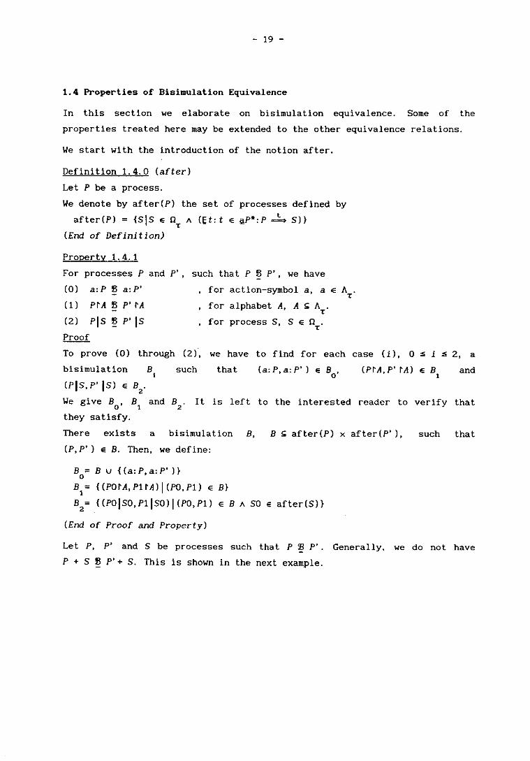
1.4 Properties of Bisimulalion Equivalence

In this section we elaborate on bisimulation equivalence. Some of the

properties treated here may be extended to the other equivalence relations.

We start with the introduction of the notion after.

Definition 1.4.0 (after)

Let P be a process.

We denote by after(P) the set of

after(P) = {SiS e Qy A (Et:t e

(End of Definition)

processes defined t gP':P ~ S)}

Property 1. 4.1

For processes P and p'. such that P ~ P' , we have

(0) a:P B a:P' for action-symbol a, a

(1) nA B P' tA for alphabet A, A ~ A . y

(2 ) piS ~ p'IS for process S, S e Q. y

Proof

by

eA. y

To prove (0) through (2 l, we have to find for each case U), O:s i :s 2, a

bisimulation

(piS, p'IS) e B2

B I

such that (a:P,a:P') e Bo

' (PtA, P' tAl e B , and

We give B , Band B2

. It is left to the interested reader to verify that o , they satisfy.

There exists a bisimulation B, B ~ after(P) x after(P'), such that

(P,P') e B. Then, we define:

BO= B u {(a:P,a:P')}

B,= {(POtA,P1tA) I (PO,P1) e B}

B2= {(POISO,P1IS0) I (PO,P1) e B A SO E after(S)}

(End of Proof and Property)

Let P, P' and S be processes such that P 7l P'. Generally, we do not have

P + S B P'+ S. This is shown in the next example.

- 20 -

Example 1. 4. 2

Let PO and Pl be processes with alphabet {b} and whose state graphs are drawn

in Figure 1.4. O.

r-·.·.-.·--· .. -.----.--··i 'PO 'Pl

IT r--·Ib • _. __ ...... _ ...... _ .. __ ... _._.J •

Ib I • . ... _ .... _ ...... __ .. _ ......... _---_.j

Figure 1.4.0: The state graphs of processes PO and Pl.

There exists a bisimulation such that PO B P1. This bisimulation is made

explicit in Figure 1. 4. 0 by drawing for each pair of processes in the

bisimulation a dotted line between the with these processes corresponding

vertices.

Consider, furthermore, the process S, S: <Z,{c},{(Z,c:ZO), (ZO, NIL)}>. The

state graphs of PO + Sand Pl + S are drawn in Figure 1.4.1.

PO + S Pl + S

Yj 0

.~ c b c

• • Figure 1.4.1: The state graphs of processes PO + Sand Pl + S

Consider the vertex that can be reached in the state graph of PO + S by

performing an initial T action. The process associated with that vertex is

not bisimulation equivalent with any of the processes that correspond to the

vertices of the state graph of Pl + S. Hence, ,(PO ~ Pl).

(End of Example)

Property 1.4.3

Let PO and Pl be processes, and let A be an alphabet such that aPO n aPl ~ A.

We have:

(POlpl)tA ~ (POtA)I(PltA)

Proof

A bisimulation B that ensures the above is:

- 21 -

B = {«plp'ltA, (PtA)I(P'tA»lp e after(PO) A P'e after(Pll}

We will prove that this is indeed a bisimulation.

Let TO and TO' be elements of after(PO), let T1 and n' be elements of

after(P1), and let trace r be an element of A*. We derive

(Toln) tA ~ (TO'ln') tA

= { Definition hiding }

(Es:s e (aTO u aT1)* A stA = r: (TOIT1)

= { Definition composition}

• """"* (TO'ln'»

(Es,t,u:s e (aTO u aT1)* A stA = rAt = staTO A u = staT1

:TO ~ TO' A T1 ~ T1')

= { note }

r e «aTO u an) () A)* A (Et:t e aTO* A ttA rtaTO:TO t = """"* A (Eu: u e an* A utA = rtaT1:T1 ~ T1')

= { Definition hiding }

TO' )

r e «aTO u an) () A)* A TOtA rtaTO, TO' tA A T1tA rtaT1, T1' tA

= { r e A*, Definition composition}

(TOtAlntA) ~ (TO' tAln' tAl

Note

For traces t and u such that t e aTO*, u e aT1*, ttA = rtaTO and utA = rtaT1,

we clarify the implication:

TO ~ TO' A T1 ~ T1' Are «aTO u aT1) () A)*

(Es:s e (aTO u aT1)* A stA = rAt = staTO A u = staT1 t u :TO ==* TO' A T ==* T1')

Its validity is based upon the following observation. Let qO and q1 be

traces. The set that consists of the symbols out of which qO is composed is

denoted by sym(qO). Similarly, we define sym(q1). Then, we have

=

qOtsym(q1) = q1tsym(qO)

(Eq2:q2 e (sym(qO) u sym(q1»* A sym(q2) = sym(qO) u sym(q1)

:q2tsym(qO) = qO A q2tsym(q1) = q1)

This property is known as the Lift Theorem, and its proof can be found in

[5, p8-9).

- 22 -

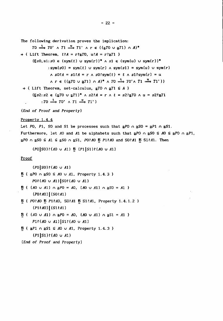
The following derivation proves the implication:

TO ~ TO' A T1 ~ T1' Are «9TO u 9T1) n A)­

~ { Lift Theorem, ttA = rt9TO, utA = rt9T1 }

(EsO,sl:s0 e (sym(t) u sym(r»- A sl e (sym(u) u sym(r»­

:sym(sO) = sym(t) u sym(r) A sym(sl) = sym(u) u sym(r)

A sOtA = sltA = r A sOtsym(t) = t A sltsym(r) = u

Are «9TO u 9T1) n A)- A TO ~ TO'A T1 ~ T1'»

~ { Lift Theorem, set-calculus, 9TO n 9T1 ~ A }

(Es2:s2 e (9TO u 9T1)- A s2tA = rAt = S2t9TO A u = s2t9T1

:TO ~ TO' A T1 ~ T1')

(End of Proof and Property)

Property 1. 4. 4

Let PO, P1, SO and Sl be processes such that 9PO n ~SO = ~P1 n 9S1.

Furthermore, let AO and A1 be alphabets such that 9PO n 9S0 ~ AO ~ ~PO n ~P1,

~PO n 9S0 ~ A1 ~ gSO n 9S1, POtAO ~ P1tAO and SOtA1 B SltA1. Then

(POISO)t(AO u A1) ~ (P1IS1)t(AO u A1)

(POISO)t(AO u A1)

~ { ~PO n ~SO ~ AO u A1, Property 1. 4.3 }

POt(AO u A1)ISOt(AO u A1)

~ { (AO u A1) n 9PO = AO, (AO u A1) n 9S0 = A1 }

(POtAO) I (SOtA1)

~ { POtAO ~ P1tAO, SOtA1 ~ SltA1, Property 1.4.1.2 }

(P1 tAO) I (Sl tAl)

~ { (AO u A1) n 9PO = AO, (AO u A1) n 9S1 = A1 }

P1t(AO u A1)IS1t(AO u A1)

~ { 9P1 n ~Sl ~ AO u A1, Property 1.4.3 }

(P1IS1)t(AO u Al)

(End of Proof and Property)

2. DEADLOCK

2.0 Introduction

The phenomenon deadlock is treated in many articles and books concerning

parallelism. Informally, it may be defined by:

'Given a set of concurrently running mechanisms. This system has

danger of deadlock if it may stop while some of its components

still want to continue.'

Applying this informal definition to a system built out of concurrently

running mechanisms that never stop, we may phrase that such a system has

danger of deadlock alternatively:

'The system may stop.'

The latter formulation is frequently used in the literature, cf [3).

We continue with an example of a system that has danger of deadlock.

Example 2.0.0

Consider the three processes 00, RO and 50 with ~OO = {aO,bO}, ~RO = {al,bl}

and ~50 = {bO,bl}. Their state graphs are presented in Figure 2.0.0.

QO

[} RO 50 bO 51

o ---=.-=----+l •

Ibl Ibl [} bO • ---=.-=----+l • Ql Rl 52 53

Figure 2.0.0: The state graphs of the processes QO, RO and 50.

The process U is the composition of these processes, i.e. U = C({QO,RO,50}).

U (Figure 2.0.1) may be viewed as the specification of a system consisting of

two work-stations (specified by 00 and RO) and one computer (specified by

50). The action-symbols of ~(C({OO,RO,50}» correspond to the following

actions:

- 23 -

- 24 -

aO: a file is placed in the memory of the work-station specified by QO. bO: a file in the memory of the work-station specified by Ql is updated

by the computer.

al: as aO but for the work-station specified by Rl.

bl: as bO but for the work-station specified by Rl.

The system stops after it has performed six actions. Then, each of the

work-stations has a file in its memory that needs to be updated by the

computer. Hence, the system has danger of deadlock.

(End of Example)

(OOIROISO) (QlIROISO) (OOIROISl) (Ql!ROISll U:

aO bO aO 0 ) . ) . ) .

all all all all

(ooIRqSO) (QqRqsO) (oolRqSll (QqRqSll aO bO aO • ) . ) . ) .

bll bll bll bll

(OOI RO IS2) (Q1 IRO IS2) (QOIRO IS3) (Qq Ro IS3) aO bO aO • ) . ) . ) .

all all all all

aO bO aO • ) . ) . ) . (QOIRl IS2) (QqRqS2) (ooIRqS3) (QqRqS3)

Figure 2.0.1: The state graph of process u.

From the processes 00, RO, SO and U, it can be derived that the system in the

above example has danger of deadlock. This is made explicit in the following

sections.

We conclude this section with some notions needed throughout the remainder of

this report.

First, the notion successor-set is redefined. In section 1. 3. 2 the

successor-set of a process denotes the maximal set of non T actions this

-----,-_ ..

- 25 -

process may perform next. Henceforth, it is defined by:

Succ(P) = {ala e A A (EP':P'e after(P) A P ~ P')} T

We say that P is non-terminating if and only if for each PO, PO e after(P),

Succ(PO) ~ 121.

Let X be a set of processes in which no two elements have the same alphabet.

By restricting ourselves to processes in Q, the definition of composition T

states that with each process T, T e after(C(X)), several sets of processes

may be associated. Informally, each of these sets denotes the states that the

components of system X may be in, while the composite is in state T. In the

sequel, we wish to address each process in after(C(X)) together with all its

corresponding sets of processes. Therefore, the notion after is modified.

Each process U, U e after(C(X)), is assumed to occur as many times in

after(C(X)) as there are 'sets of processes associated with U. Hence,

after(C(X)) becomes a bag. We implicitly assume some sort of one to one

mapping between the processes U in after(C(X)) and the with U associated sets

of processes. Then, e(V,P,X), P e X and Ve after(C(X)), denotes the unique

element of after(P) that occurs in the with V associated set of processes.

2.1 Locked and Lockfree

Throughout the remainder of this report, X is a set of processes and P is an

element of X. Furthermore, only processes Q with a finite number of elements

in the set after(Q) are considered.

We start by formalizing the informal definition of danger of deadlock by the

concept lockfree.

Definition 2.1.0 (locked)

locked(P,X)

=

(ET:T e after(C(X)):Succ(T) # 121 A Succ(e(T,P,X)) ~ 121)

(End of Definition)

Definition 2.1.1 (lockfree)

lockfree(X) = (BP:P e X:~locked(P,X))

(End of Definition)

If ~lockfree(X) holds, we say that the system specified by X has danger of

peiqg locked.

Property 2.1.2

lockfree(e)

lockfree ({P})

- 26 -

, for any process P

(0)

(1)

(2) C(X) is non-terminating ~ lockfree(X)

(End of Property)

Property 2.1.3

Let PO be a process in after(C(X». We then have

Succ(PO) ~ (UT:T e X:Succ(e(PO,T,X»)

Proof

a e Succ(PO)

= { Definition Succ(P) }

a e {bib e AT A (EP':P'e after(PO):PO ~ P')}

= { set calculus }

a e A A (EP':P'e after(C(PO»:PO ~ P')} T

~ { PO e after(C(X), Definition composition}

(ET:T e X:a E A A (EP':P'E after(T):e(PO,T,X) ~ P')} T .

= { Definition Succ(P) }

(ET:T E X:a E Succ(e(PO,T,X»)

= { set calculus }

a E (UT:T E X:Succ(e(PO,T,X»)

(End of Proof and Property)

Property 2.1.4

lockfree(X)

=

1 >

(BPO:PO E after(C(X»: (Succ(PO) = e) = (BT:T E X:Succ(e(PO,T,X» = e»

lockfree(X)

= { Definition lockfree }

(BT:T e X:~locked(T,X»

= { Definition locked}

(BT:T E X: (BPO:PO E after(C(X»:Succ(PO) * e v Succ(e(PO,T,X»

= { predicate calculus }

(BPO:PO E after(C(X»:Succ(PO) = " ~ (BT:T E X:Succ(e(PO, T,X»

= { Property 2.1.3 }

= e))

= e»

- 27 -

(BPO:PO e after(C(X»: (Succ(PO) = 0) = (BT:T e X:Succ(e(PO,T,X» = 0»

(End of Proof and Property)

Theorem 2.1.5

Let X be a set of processes. For each process T, T e X, T denotes the process

C(X\{T}). Then A

lockfree(X) =(BT:T e X:lockfree({T,T}»

lockfree(X)

= { Definition lockfree }

(BT:T e X:,locked(T,X»

= { note } A A

(BT:T e X:,locked(T,X» A (BT:T e X :,locked(T,{T,T}» A A

= { C(X) = C({T,T}), T e {T,T}, Definition locked} A A A

(BT:T e X:,locked(T,{T,T}» A (BT:T e X:,locked(T,{T,T}»

= { predicate calculus, Definition lockfree } A

(BT:T e X:lockfree({T,T}»

We prove: A A

(BT:T e X:,locked(T,X» ~ (BT:T e X:,locked(T,{T,T}»

For any T, T E X, we derive: A A

locked(T, {T, T})

= { Definition locked} A A A

(EPO:PO e after(C{T,T}):Succ(PO) = 0 A Succ(p(PO,T,{T,T}» * 0)

~ { C({T,T}) = C(X), Property 2.1.3 }

(EPO:PO e after(C(X»:Succ(PO) = 0 A (EU:U e X\{T}:Succ(e(PO,U,X» * 0»

= { predicate calculus, Definition locked}

(EU:U e x\{T}:locked(U,X»

~ { predicate calculus }

(EU:U e X:locked(U,X»

(End of Proof and Theorem)

- 28 -

Example 2.1.6

Consider the three processes 00, RO and SO that were introduced in example

2.0.0.

Let X = {OO,RO,SO}, and let PO be the process that corresponds to the

composition of the elements in {Q1,R1,S3}.

As it can be derived from Figure 2.0.1, PO is an element of after(C(X».

Since Succ(PO) = e and Succ(Q1) * e, we conclude locked(OO,X) and

locked (00, {OO,C(x\{OO})}).

(End of Example)

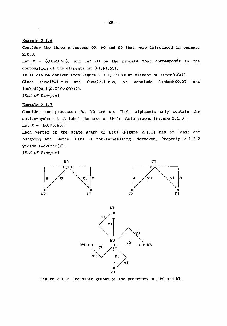
Example 2.1.7

Consider the processes va, va and WO. Their alphabets only contain the

action-symbols that label the arcs of their state graphs (Figure 2.1.0).

Let X = {VO,VO,WO}.

Each vertex in the state graph of C(X) (Figure 2.1.1) has at least one

outgoing arc. Hence, C(X) is non-terminating. Moreover, Property 2.1.2.2

yields lockfree(X).

(End of Example)

UO

V2 VI

WI

• V2

vo

• V1

Figure 2.1.0: The state graphs of the processes va, va and WI.

- 29 -

(U2IVOIW2) (UlI VO IWll C(X) :

:y.~;y.~ (U2IV2IWO) a (UOIVOIWO) b (UIIVIIWO)

• ) 0 E •

~/O~/, • •

(UOIV2IW4) (UOIVIIW3)

Figure 2.1.1: The state graph of process C(X).

2.2 Construction of lockfree systems

It is difficult to determine whether a system that is specified by a set X of

processes has danger of being locked. If X only consists of non-terminating

processes, we may proceed as in example 2.1.7. A more general method is

presented in this section.

Lemma 2.2.0

Let X and Y be sets of processes such that X A Y = 0 and lockfree(X). Then

~locked(C(X),{C(X),C(Y)}) = (BT:T e X:~locked(T,X u Y))

~locked(C(X),{C(X),C(Y)})

= { Definition locked}

(BPO:PO e after(C({C(X),C(Y)}))

:Succ(PO) * 0 v Succ(e(PO,C(X),{C(X),C(Y)})) = 0)

= { lockfree(X) }

(BPO:PO e after(C({C(X),C(Y)}))

:Succ(PO) * 0 v (BT:T e X:Succ(e(e(PO,C(X),{C(X),C(Y)}),T,X)) = 0))

= { C({C(X),C(Y)}) = C(X u y) }

(BPO:PO e after(C(X u Y))

:Succ(PO) * 0 v (BT:T e X:Succ(e(PO,T,X u Y)) = 0))

= { predicate calculus, Definition: locked}

(BT:T e X:~locked(T,X u y))

(End of Proof and Lemma)

- 30 -

The following theorem shows how to build larger lockfree systems out of

smaller ones.

Theorem 2.2.1

Let both X and Y be a set of processes such that X n Y = 0, lockfree(X) and

lockfree(Y). We have:

lockfree({C(X),C(Y)} = lockfree(X u Y)

lockfree({C(X),C(Y)})

= { Definition lockfree }

~locked(C(X),{C(X),C(Y)}) A ~locked(C(Y),{C(X),C(Y)})

= { Lemma 2.2.0 }

(BPO: PO e X:~locked(PO,X v Y)) A (BPO:PO e Y:~locked(PO,X v Y))

= { predicate calculus, Definition lockfree }

lockfree(X v Y)

(End of Proof and Theorem)

Using Theorem 2.2.1 and Properties 2.1. 2.1 and 2.1.2.2, we may be able to

determine for a finite set X of processes whether lockfree (X) holds. To

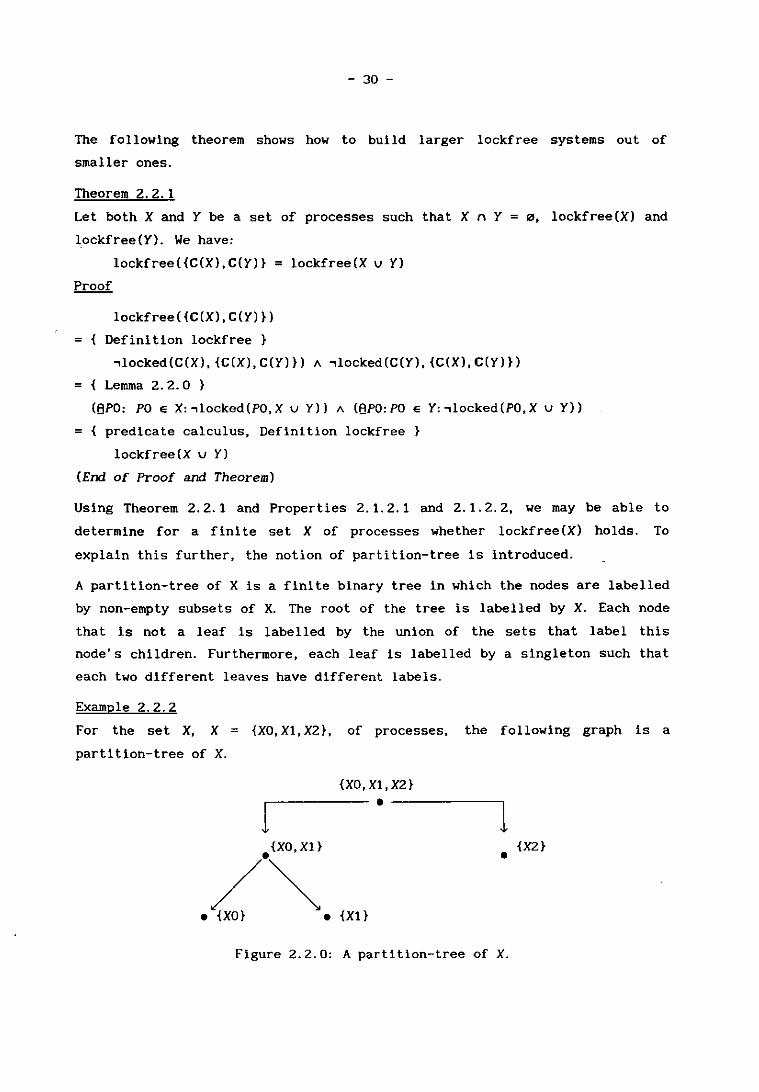
explain this further, the notion of partition-tree is introduced.

A partition-tree of X is a finite binary tree in which the nodes are labelled

by non-empty subsets of X. The root of the tree is labelled by X. Each node

that is not a leaf is labelled by the union of the sets that label this

node's children. Furthermore, each leaf is labelled by a singleton such that

each two different leaves have different labels.

Example 2.2.2

For the set X, X = {XO, Xl, X2}, of processes, the following graph is a

partition-tree of X.

{XO,X1,X2}

1....---·

/~ • {XO} • {Xl}

1 •

Figure 2.2.0: A partition-tree of X.

{X2}

- 31 -

Notice that several partition-trees of X exist.

(End of Example)

From Property 2.1.2.1, we infer that the singletons that label the leaves of

a partition-tree of X are lockfree. If such a tree can be traversed from

leaves to root using Property 2.1.2.2 and Theorem 2.2.1, lockfree(X) holds.

Example 2.2.3

Consider the processes PO, QO, RO and SO. Their alphabets only contain those

action-symbols that label the arcs in their state graphs (Figure 2.2.1)

PO o

QO RO SO

/j. • E b •

[} [} [} P2 Q1 R1 S1

Figure 2.2.1: The state graphs of processes PO, QO, RO and SO.

Let X = {PO,QO,RO,SO}.

Lockfree(X) can be proven using the following partition-tree.

{PO,QO,RO,SO}

!r--- • ---""1

~~R;;}1 f{Qo~s;;}1 •

{PO} •

{RO} •

{QO} •

{SO}

Figure 2.2.2: A partition-tree of X.

Since ilPO " ilRO = 121 and PO as well as RO is non-terminating, C( {PO, RO}) is

non-terminating. Property 2.1.2.2 then states lockfree({PO,RO}).

Similar reasoning yields lockfree({QO,SO}).

It is easily verified that lockfree({C({PO,RO}),C({QO,SO})}).

Hence, we may conclude from Theorem 2.2.1 that lockfree(X) holds.

(End of Example)

The above strategy does not always work. There are lockfree systems for which

a proper partition-tree can not be found. The following example shows such a

system.

- 32 -

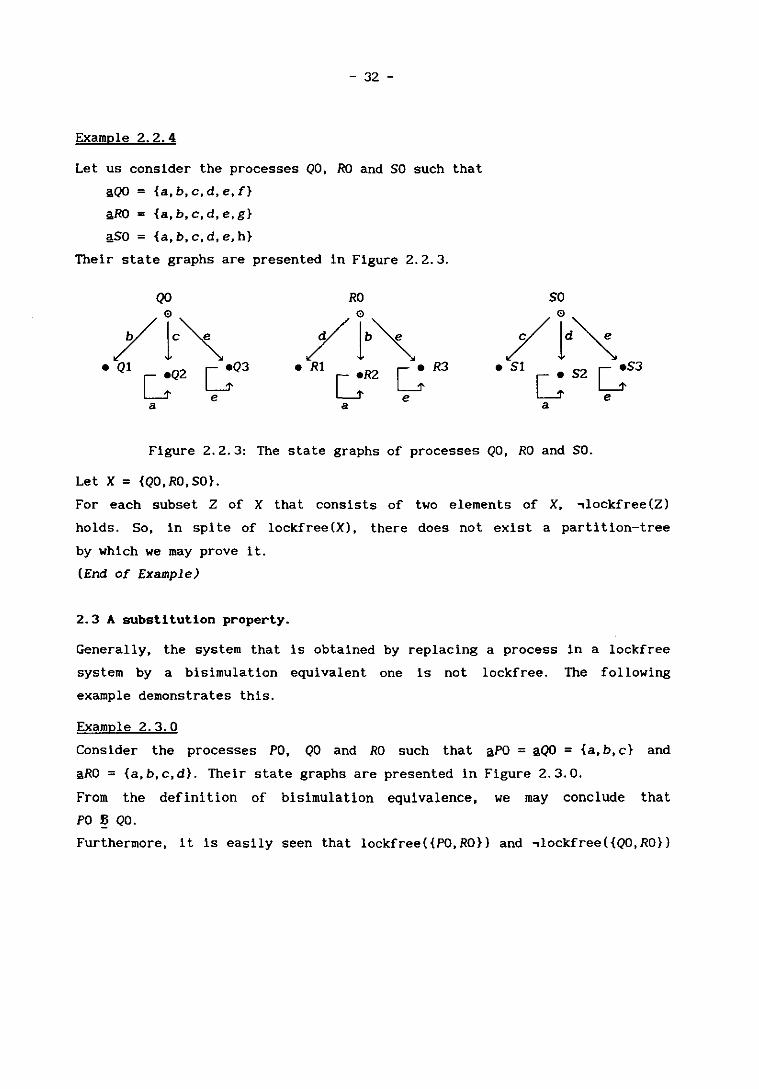
Example 2.2.4

Let us consider the processes QO, RO and SO such that

gQO = {a,b,c,d,e,f}

gRO = {a,b,c,d,e,g}

~SO = {a,b,c,d,e,h}

Their state graphs are presented in Figure 2.2.3.

QO RO

R3

a a

SO

/Id~ • S1 c..; S2 ~S3

a

Figure 2.2.3: The state graphs of processes QO, RO and SO.

Let X = {QO,RO,SO}.

For each subset Z of X that consists of two elements of X, ,lockfree(Z)

holds. So, in spite of lockfree (X), there does not exist a partition-tree

by which we may prove it.

(End of Example)

2.3 A substitution property.

Generally, the system that is obtained by replacing a process in a lockfree

system by a bisimulation equivalent one is not lockfree. The following

example demonstrates this.

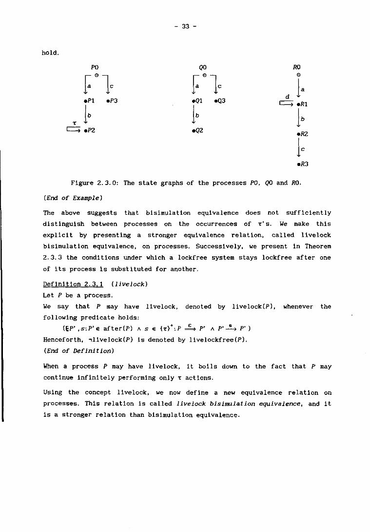
Example 2.3.0

Consider the processes PO, QO and RO such that ~PO = gQO = {a,b,c} and

~RO = {a,b,c,d}. Their state graphs are presented in Figure 2.3.0.

From the definition of bisimulation equivalence, we may conclude that

PO ~ QO.

Furthermore, it is easily seen that 10ckfree({PO,RO}) and ,lockfree({QO,RO})

- 33 -

hold.

PO QO RO

fa 01C

° d la

eQ1 eQ3 '==+ eR1

Ib Ib eQ2 eR2

Ic eR3

Figure 2.3.0: The state graphs of the processes PO, QO and RO.

(End of Example)

The above suggests that bisimulation equivalence does not sufficiently

distinguish between processes on the occurrences of T'S. We make this

explicit by presenting a stronger equivalence relation, called livelock

bisimulation equivalence, on processes. Successively, we present in Theorem

2.3.3 the conditions under which a lockfree system stays lockfree after one

of its process is substituted for another.

Definition 2.3.1 (livelock)

Let P be a process.

We say that P may have livelock, denoted by livelock(P), whenever the

following predicate holds:

(EP' ,s:P'e after(P) A s e {T}+:P ~ P' A P'~ P')

Henceforth, ,livelock(P) is denoted by livelockfree(P).

(End of Definition)

When a process P may have livelock, it boils down to the fact that P may

continue infinitely performing only T actions.

Using the concept l1velock, we now define a new equivalence relation on

processes. This relation is called livelock bisimulation equivalence, and it

is a stronger relation than bisimulation equivalence.

- 34 -

Definition 2.3.2 (livelock bisimulation equivalence)

Two processes PO and PI are called livelock bisimulation equivalent, denoted

by PO !!L PI, if and only if there exists a bisimulation /3 such that

(PO,Pl) e /3 and for all pairs (U,V) in /3 livelock(U) = livelock(V).

(End of Definition)

Without proof, we state that by restricting ourselves to processes P with

after(P) finite, all properties derived in section 1.4 also hold for livelock

bisimulation equivalence.

Theorem 2.3.3

Let TO, Tl and S be processes such that ~TO n ~S = ~Tl n ~S.

Furthermore, let A be an alphabet such that ~TO n ~S !;; A !;; ~TO n ~Tl and

TO~A !!L Tl~A. We have:

lockfree({TO,S}) = lockfree({Tl,S})

Proof

Since TO~A !!L Tl~A, there exists a proper bisimulation /3 for it.

According to Property 1.4.4 (TOIS)t(A u ~S) !!L (T1IS)t(A U ~S).

Applying Property 1.4.1.2 makes it obvious that a corresponding bisimulation

r is: {((POISO), (PtlSO»1 (PO,Pl) e /3 A SO e after(S)}

We will only derive locked(TO,{TO,S}) = locked(Tl,{Tl,S}), because then the

proof of locked(S,{TO,S}) = locked(S,{Tl,S}) will be trivial.

locked(TO, {TO,S})

= { Definition locked}

(EP:P e after(C({TO,S}»:Succ(P) = 0 A Succ(e(P,TO,{TO,S}» ~ 0)

= { set calculus, Definition composition}

(EP:P e after(C({TO,S}»

:Succ(P) = 0 A (Ea:a e ~TO n ~S:a e Succ(e(P,TO,{TO,S}»»

= { note }

(EP:P e after(C({Tl,S}»

:Succ(P) = 0 A (Ea:a e ~Tl n ~S:a e Succ(e(P,Tl,{Tl,S}»»

= { set calculus, Definition composition}

(EP:P e after(C({Tl,S}»:Succ(P) = 0 A Succ(e(P,Tl,{Tl,S}» ~ 0)

= { Definition locked}

locked(Tl,{Tl,S})

- 35 -

Note

We prove that

(EP:P e after(C({TO,S}»

:Succ(P) = 0 A (Ea:a e ~TO n ~S:a e Succ(e(P,TO,{TO,S}»»

(EP:P e after(C({Tl,S}»

:Succ(P) = 0 A (Ea:a e aTl n as:a e Succ(e(P,Tl,{Tl,S}»»

For reasons of symmetry, the converse is omitted.

Let P be a process in after<C( {TO, S}» such that Succ(P) = 0 and

Succ(e(P,TO,{TO,S}» contains an element of aTO n as.

From (TOIS)t(A v as) ~L (Tl!S)t(A vaS) and P e after(C({TO,S}»). it is

inferred that there exists a process Q, Q e after(C({Tl,S}», such that:

(Pt(A v as),Qt(A v ~S» e r

Since Succ(P) = 0 and aTl n as ~ A, the definitions of composition, hiding

and live lock bisimulatlon equivalence state that there exists a process Q'

such that Q ~ Q' (t e (~Tl\A)'), (Pt(A v as»,Q't(A v ~S» e rand

Succ(Q') = 0.

According to the definition of r, processes PO and a process QO exist such

that PO = e(P,TO,{TO,S}) and QO = e(Q',Tl,{Tl,S}).

Since ~TO n as ~ A and Succ(PO) contains an element of aTO n as, Succ(POtA)

contains an element of ~TO n as. Furthermore, it may be concluded from

Succ(Q') = 0 and the definitions of composition and hiding that

Succ(QOtA) ~ aTl n ~S.

Then, we infer from (POtA,QOtA) e ~ and aTO n as = ~Tl n ~S that Succ(QOtA)

contains an element of aTl n as. Hence Succ(QO) contains an element of

aTl n as.

(End of Proof and Theorem)

- 36 -

Theorem 2.3.3 may be generalized.

Theorem 2.3.4

Let X be a set of processes, let P be an element of X, and let Q be a

process. Assume that Q ~ X\{P} and aC(X\{P}} naP = gC(Y\{Q}) n aQ.

Furthermore, let A be an alphabet such that aC(X\{P}) n aP ~ A ~ aP n aQ and

PtA ~L QtA.

If Y denotes the set X of processes in which P is substituted for Q, we have

lockfree(X) = lockfree(Y)

lockfree(X)

= { Theorem 2. 1. 5 }

(ST:T e X:lockfree({T,C(x\{T})}))

= { note },

(ST:T e X:lockfree({T,C(y\{T})}))

= { Theorem 2. 1. 5 }

lockfree(Y)

Note

This equality is based upon two observations.

First: C(x\{P}) = C(Y\{Q}), ptA ~L QtA and Theorem 2.3.3 yields

lockfree({P,C(X\{P})}) = lockfree({Q,C(Y\{Q})})

Second: Let T e x\{P} (and thus T e Y\{Q}).

Easily, it is seen that aT n aC(x\{T}) = aT n aC(y\{T}).

Furthermore, notice that aC(x\{T,P}) u A = i1,C(y\{T,Q}) u A.

and i1,T n i1,C(x\{T}) ~ aC(x\{T,P}) u A ~ aC(x\{T}) n aC(y\{T}).

From Property 1.4.2.2 and Property 1.4.3, we infer that

C(x\{T})t(aC(x\{T,P}) u A) ~L C(y\{T})t(i1,C(y\{T,Q}) u A)

Then Theorem 2.3.3 states:

lockfree({T,C(x\{T})}) = lockfree({T,C(y\{T})})

(End of Proof and Theorem)

P.J. de Graaff [2) has shown that within each class of bisimulation

equivalent processes there exists a unique process Whose state graph has the

smallest number of vertices and arcs from all the other processes. An

algorithm exists that computes for a given process this unique

representative. The algorithm is called the minimization algorithm for

bisimulation equivalence. Without going into further details, we state that

- 37 -

the above can be extended to livelock bisimulation equivalence.

The complexity of computing lockfree(X) is proportional to the total number

of arcs and vertices of the state graphs that correspond to the processes in

X. Theorem 2.3.4 and the minimization algorithm for livelock bisimulation

equivalence may be used to reduce the complexity of computing lockfree(X).

2.4 Deadlockfree

In section 2.0, we informally defined danger of deadlock in a system built

out of concurrently running mechanisms. Unfortunately, this definition does

not cover all the aspects that are generally implied by danger of deadlock.

Consider a system built out of two or more SUbsystems. Each two subsystems do

not interfere in one another's behaviour. Intuitively, this system has danger

of deadlock if and only if one or more of the subsystems have danger of

deadlock. Yet, let one of these separate subsystems have danger of deadlock

while another never stops. Then, the composite system never stops. Although

this system has danger of deadlock, the informal definition states otherwise.

The above and Property 2.1.2.2 yields that the concept lockfree is a to weak

predicate to state whether or not a system has danger of deadlock. Therefore,

we present in this section an other concept, called deadlockfree, that

resolves our objections against the concept lockfree.

Definition 2.4.0 (connected)

connected (X)

=

(BY:Y ~ X A Y ¢ 0 A Y ¢ X:gC(Y) n gC(x\Y) ¢ 0 )

(End of Definition)

Definition 2.4.1 (maximal connected)

Let X be a set of processes, and let Y be a subset of X. We define:'

maximal connected(Y,X) = connected(Y) A (BP:P e x\Y:, connected(Y v {P}»

(End of Definition)

Definition 2.4.2 (deadlockfree)

deadlockfree(X) = (BY:Y ~ X A maximal connected(Y,X):lockfree(Y»

(End of Definition)

Property 2.4.3

deadlockfree(X) • lockfree(X)

(End of Property)

- 38 -

3. OTHER CONCEPTS

3.0 Introduction

In the previous chapter, we have introduced the concept deadlockfree to

describe the presence or absence of deadlock in a system built out of

concurrently running mechanisms. Similarly, properties related to danger of

deadlock may be formalized. In this chapter, two of these properties, called

danger of being disabled and danger of being ignored, will be presented. A

short treatment of each of them is given. For more information about these

concepts and their extensions to actions, the reader is referred to [4].

3.1 Disablefree

Consider a system that has performed actions up to some moment in time.

From this moment on, a not yet terminated component of the system can never

again participate in whatever actions the system shall perform. One might say

that this component has danger of being disabled by the system. We formalize

this property as follows:

Definition 3.1.0 (disabled)

disabled(P,X)

=

(ET: T e after(C(X)

:Succ(E(T,P,X») e P(aP n aC(X))'{{e}}

A (BT':T'e after(T):Succ(T') naP = e»

(End of Definition)

Definition 3.1.1 (disablefree)

disablefree(X) = (BP:P e X:~disabled (P,X))

(End of Definition)

The concept disablefree is stronger than the concept deadlockfree.

If we replace each occurrence of lockfree in the properties 2.1.2. a and

2.1. 2. 1 and in the theorems 2.1.5, 2.3.3 and 2.3.4 by disablefree, these

properties and theorems are still correct. Unfortunately, substituting

- 39 -

- 40 -

each occurrence of lockfree for disablefree in Theorem 2.2.1 yields a theorem

that does not hold. Hence, we do not have a construction theorem that shows

how larger disablefree systems may be built from smaller ones.

3.2 Ignorefree

A disablefree system may always perform a sequence of actions such that each

not terminated component participates in one of these actions. However, this

does not imply that for each not terminated component the system can only

perform a finite number of actions in which this component does not

participate.

When a system may continuously perform actions in which a not terminated

component does not participate, we say that that component may be ignored by

the system. This will now be formalized.

Definition 3.2.0 (ignored)

Let X be a set of processes and let P be a process in X.

For each process T, T E after(C(X», Tp denotes

C({Qi (EV:V E X'-{P}:Q = e(T,V,X)}).

Then, we define:

ignored(P,X) = locked(P,X) v processlivelock(P,X)

where processlivelock(P,X) denotes:

the

(ET:T E after(C(X»:Succ(e(T,P,X» ~ 0 A livelock(T taC(X'-{P}») p

(End of Definition)

Definition 3.2.1 (jgnorefree)

ignorefree(X) = (BT:T E after(C(X»:,ignored(T,X»

(End of Definition)

process

When (BT:T E X:,processlivelock(T,X» is abbreviated by systemlivelockfree(X)

, the following theorem is self evident.

Theorem 3.2.2

ignorefree(X) = lockfree(X) A systemlivelockfree(X)

(End of Theorem)

Furthermore, it is easily seen that ignorefree is a stronger concept than

disablefree.

In Properties 2.1. 2. 0 and 2.1. 2.1 and in Theorem 2.1.5, all occurrences of

lockfree may be replaced by systemlivelockfree, without changing the

- 41 -

correctness of these properties and theorems. If we add to Theorem 2.2.1 that

C(X) and C(Y) are non-terminating, to Theorem 2.3.3 that both TO and T1 are

non-terminating and to Theorem 2.3.4 that P and Q are non terminating, these

modified theorems also hold if we replace in them all occurrences of lockfree

by systemlivelockfree.

Theorem 3.2.2 ensures that all the modified properties and theorems that are

presented in this section also hold if we replace in them all occurrences of

systemlivelockfree by ignorefree.

This section is concluded by presenting a theorem that shows how a larger

disablefree system may be built out of two ignorefree systems.

Theorem 3.2.3

Let X and Y be processes such that C(X) and C(Y) are non-terminating,

X n Y = ~, and ignorefree(X) and ignorefree(Y). Then

disablefree({C(X),C(Y)}) = disablefree(X u Y)

(End of Theorem)

4. CONCLUSIONS

In this report, we have combined mayor features of CCS and Trace Theory into

a new formalism. The central notion in this formalism is called process. It

is used to specify the behaviour of systems. Like CCS, we do not exclude

non-determinism in the specification of the behaviour of a system.

Furthermore, the specification of the behaviour of a larger system is

obtained from the specifications of the system's components in a way similar

to the one used in Trace Theory. We have introduced the T-action. Contrary

to CCS, T-actions are not used to specify the interaction between two

systems. They are only used to abstract from certain actions of a system.

Besides presenting a formalism, we have also given a summary of some

equivalence relations on the universe of processes. Furthermore, a concept is

presented that describes when a system has danger of deadlock. A theorem is

given that shows how larger deadlockfree systems may be built out of smaller

ones. Conditions are stated under which a system without danger of deadlock

stays deadlockfree after one of its processes is substi tuted for another.

Finally, the same is performed for other deadlock-like properties.

Further research will be focused on putting the results in this report into

practice. Concretely, this means that the investigation alms to embed the

results into some sort of top-down design trajectory for a class of

concurrent systems. The important aspect in this trajectory will be a

meaningful decomposition of a system that is hard to design into components

that are easier to design. By a meaningful decomposition, we emphasize the

point that the composite behaviour of the components has to correspond to the

behaviour of the system to be designed. For instance, decomposition may not

introduce deadlock.

Acknowledgements:

The author is indebted to anyone who somehow has contributed to this report.

Special thanks are due to P.J. de Graaff, A.F.P. van Putten, H.H.M. van de

Weij and M.R.M. Winter for their fruitful comments.

- 42 -

5. REFERENCES

[1] Brookes, S.D. and C.R. Rounds

Behavioural Equivalent Relations Induced By Programming Logics

Internal report (CMU-CS-83-112), Department of Computer Science,

Carnegie Mellon University,

Pittsburgh, Pennsylvania, 1983

[2] Graaff, P.J. de,

Some notes on observation equivalence

Faculty of Electrical Engineering,

Digital Systems Group (EB),

Eindhoven University of Technology,

Personal communications

[3] Hoare, C.A.R.

Communicating Sequential Processes,

Prentice-Hall International Series in Computer Science,

Englewood Cliffs, New Jersey, 1985

[4] Huis in 't Veld, R.J.

Deadlock properties expressed in terms of Trace Theory

M. Sc. -thesis, Faculty of Mathematics and Computing Science,

Eindhoven University of Technology, 1987

[5] Kaldewaij, A.

A Formalism for Concurrent Processes

Ph. D. -thesis,

Eindhoven University of Technology, 1986

[6] Milner, R.

A Calculus of Communicating Systems

Lecture Notes in Computer Science, vol. 92

Berlin: Springer, 1980

- 43 -

£indhoven University of Technology Research Reports faculty of Electrical Engineering

ISSN 0167-9708 Coden: TEU£DE

( 1711

( 1721

(173 )

(174)

( 175)

( 176)

( 177)

(178)

(179)

(1801

(181 )

Monnee, P. and M.H.A.J. Herben MLITJnn5LE-8EAM GROUNOSTAT~FLECTOR ANTENNA SYSTEM: A preliminary study. EUT Report 87-E-171. 1987. ISBN 90-6144-171-4

Bastiaans, M.J. and A.H.M. Akkermans ERROR REDUC110N IN lWO-OIMENSloNAl PULSE-AREA MOOULA110N, WIIH APPLICATION TO COMPUTER-GENERATED TRANSPARENCIES. EUI Report 87-E-172. 1987. ISBN 90-6144-172-2

Zhu Yu-Cai on-A BDUND OF THE MODELLING ERRORS OF BLACK-BOX EUT Report 87-E-173. 1987. ISBN 90-6144-173-0

TRANSFER FUNCTION ESTIMATES.

Berkelaar, M.R.C.M. and J.F.M. Theeuwen TECHNOLOGY MAPPING FROM BOOLEAN EXPRESSIONS 10 STANDARD CELLS. EUT Report 87-E-174. 1987. ISBN 90-6144-174-9

Janssen, P.H.M. FURl HER RESULTS ON THE McMILLAN DEGREE AND THE KRONECKER EUT Report 81-E-175. 1987. ISBN 90-6144-175-7

INDICES OF ARMA MODELS.

Janssen, P.H.M. and P. Stoiea, T. Soderstrom, P. E~khOff MODEL STRUCTURE SELECTI~ MULTIVARIABLE SYSTEM BY CROSS-VALIDATION METHODS. EUT Report 87-E-176. 1987. ISBN 90-6144-176-5

Stefanov, B. and A. Veefkind, L. Zarkova ARCS IN CESIUM SEEDED NOBLE GASES RESULTING FROM A MAGNETICALLY FIELD. EUT Report 87-E-177. 1987. ISBN 90-6144-177-3

Janssen, P.H.M. and P. Stoica

INDUCED ELECTRIC

ON THE EXPECTATION OF THE PRODUCT OF FOUR MATRIX-VALUED GAUSSIAN RANDOM VARIABLES. EUT Report 87-E-178. 1987. ISBN 90-6144-178-1

Lieshout, C.J.P. van and L.P.P.P. van Cinneken GM: A gate matrix layout generator. EUT Report 87-E-179. 1987. ISBN 90-6144-179-X

Cinneken, L.P.P.P. van GRIDLESS RoUTING FOR GENERALIZED CELL ASSEMBLIES: EUT Report 87-E-180. 1987. ISBN 90-6144-180-3

Report and user manual.

Bollen, M.H.J. and P.T.M. Vaessen ~NCY SPECTRA FOR ADMITTANCE ANO VOLTAGE TRANSFERS MEASUREO ON A THREE-PHASE POWER TRANSFORMER. EUT Report 87-E-181. 1987. ISBN 90-6144-181-1

(182) Zhu Yu-C.i ~CK-BOX IDENTIFICATION OF MIMO TRANSFER FUNCTIONS: Asymptotic properties of prediction error models. EUT Report 87-E-182. 1987. ISBN 90-6144-182-X

(183) Zhu Yu-C.i

(184 )

( 185)

on-THE BOUNDS OF THE MODELLING ERRORS OF BLACK-BOX MIMO TRANSFER FUNCTION ESTIMATES. EUT Report 87-E-183. 1987. ISBN 90-6144-183-8

Kadete, H. ENHANCEMENT OF HEAT TRANSFER BY CORONA WIND. EUT Report 87-E-184. 1987. ISBN 90-6144-6

Hermans, P.A.M. and A.M.J. Kwaks, r.v. Bruza, J. Di~b THE IMPACT OF TELECOMMUNICA~ON RURA~AS IN 0 ELOPING COUNTRIES. EUT Report 87-E-185. 1987. ISBN 90-6144-185-4

(186) Fu Yanhong

( 187)

THE INFLUENECE OF CONTACT SURFACE MICROSTRUCTURE ON VACUUM ARC STABILITY AND ARC VOLT AGE. EUT Report 87-E-186. 1987. ISBN 90-6144-186-2

Kaiser, F. and L. Stok, R. van den Born DESTCN AND IMPLEMENTATION OF A MODULE LIBRARY TO SUPPORT THE STRUCTURAL SYNTHESIS. EUT Report 87-E-187. 1987. ISBN 90-6144-187-0

Eindhoven University of Technoloqy Research Reports Faculty of Electrlcal Enqineerlng

ISSN 0167-9708 Coden: TEUEDE

( 188)

(189)

Jozwiak, J. THE FuLL DECOMPOSITION OF SEQUENTIAL MACHINES WITH THE STATE AND OUTPUT BEHAVIOUR REALIZATION. EUT Report 88-E-188. 1988. ISBN 90-6144-188-9

Pineda de Cyvez, J. ALWAys: A system for wafer yield analysis. EUT Report 88-E-189. 1988. ISBN 90-6144-189-7

(190) Siuzdak, J. OpllCAL COUPLERS FOR COHERENT OPTICAL PHASE DIVERSITY SYSTEMS. EUT Report 88-E-190. 1988. ISBN 90-6144-190-0

(191) Bastiaans, M.J. LOCAL-FREQUENCY DESCRIPTION OF OPTICAL SIGNALS AND SYSTEMS. EUT Report 88-E-191. 1988. ISBN 90-6144-191-9

(192)

(193)

Worm, S.C.J. AlMULTI-FREQUENCY ANTENNA SYSTEM FOR PROPAGATION EXPERIMENTS WITH THE OLYMPUS SATELLITE. EUT Report 88-E-192. 1988. ISBN 90-6144-192-7

Kersten, W.F.J. and G.A.P. Jacobs ANALOG AND DIGITAL SIMULATI~LINE-ENERGIZING OVERVOLTAGES AND COMPARISON WITH MEASUREMENTS IN A 400 kV NETWORK. EUT Report 88-E-193. 1988. ISBN 90-6144-193-5

(194) Hosselet, L.M.L.F. MARTINUS VAN MARUM: A Dutch scientist in a revolutionary time. EUT Report 88-E-194. 1988. ISBN 90-6144-194-3

(195) Bondarev, V.N.

( 196)

ON SYS1EM IDENTIFICATION USING PULSE-FREQUENCY MODULATED SIGNALS. EUT Report 88-E-195. 1988. ISBN 90-6144-195-1

Liu Wen-Jiang, Zhu Yu-Cai and Cai Da-Wei MODEL BUILDING FOR AN INGOT HEAfTNG PROCESS: Physical identification approach. EUT Report 88-E-196. 1988. ISBN 90-6144-196-X

modelling approach and