A FORMAL EVALUATION OF STORM TYPE VERSUS STORM...

A FORMAL EVALUATION OF STORM TYPE VERSUS STORM

MOTION

___________________________________

A Thesis presented to the faculty of the Graduate School at the

University of Missouri-Columbia

____________________________________________________

In Partial Fulfillment

of the Requirements for the Degree

Master of Science

_____________________________________________________

by JOSÉ MIRANDA

Dr. Neil I. Fox, Thesis Supervisor

MAY 2008

The undersigned, appointed by the dean of the Graduate School, have

examined the thesis entitled

A FORMAL EVALUATION OF STORM TYPE VERSUS STORM MOTION

presented by José Miranda,

a candidate for the degree of master of science,

and hereby certify that, in their opinion, it is worthy of acceptance.

_____________________________

Assistant Professor Neil I. Fox

_____________________________

Associate Professor Anthony R. Lupo

_____________________________ Professor Christopher K. Wikle

DEDICATED TO NORMA BERRY

JUNE 14, 1924-DECEMBER 2, 2007

AN INSPIRATION TO THOSE WHO SHE BLESSED WITH HER PRESENCE

ii

ACKNOWLEDGEMENTS

I would like to start off by thanking the Department of

atmospheric science at the University of Missouri-Columbia. My

advisor, Neil I. Fox, also deserves many thanks in providing me the

guidance I needed to complete this publication and giving me the

opportunity to continue my education. Also, many thanks go to Dr.

Patrick Market and Dr. Anthony Lupo for teaching me what I know

today in the field of atmospheric science as well as spending their time

and effort solving problems, both small and large, that have come up

along the way.

I would also like to acknowledge the organizations that funded

this research. Thanks go to the National Science Foundation and the

University of Missouri-Columbia Research Council for the approval to

conduct research on the topic of thunderstorm motion.

Furthermore, I would not have written this thesis without the

help of many undergraduate and graduate students within the

department of atmospheric science. Steven Lack’s guidance,

especially with his statistical classifier, George Limpert’s guidance with

WDSS-II and an assortment of other weather and non-weather related

programs and banter, Ali Koleiny and Chris Melick’s uncanny ability to

distract me from the rigors of my research, Rachel Redburn, Willie

iii

Gilmore, Mark Dahmer, Christopher Foltz, Brian Pettegrew, Larry

Smith, Amy Becker, Melissa Chesser, and Neville Miller, among others,

all deserve thanks for providing needed insight, and reminding me why

I want to enter this profession.

Most of all, the largest amount of thanks and appreciation go out

to my family and friends. My undergraduate mentor, Christopher

Straub, my high-school mentor, Michael Dager, and my college cross-

country teammates at Elizabethtown. My best friend, Adam Arker,

who has given me the inspiration to “go for it”, and genuinely love

what you do. My family, my mother, father, brother, there will never

be enough thanks and gratitude that will ever be expressed from me

for your love, support, and advice in making major decisions in my

life. There were times when it was really, really tough and times when

I wanted to quit but you were there. I love you all.

Finally, this thesis is dedicated to the two people who are my

life, my world, and the reason you are reading this sentence right now,

my wife Melissa and daughter Cheyenne. I owe everything I have

done, and give credit for being able to make it through graduate

school, to these two wonderful people. It was hard to become a

parent and as a couple complete our education, but it is of the utmost

importance to do so. No one else can sympathize with my

iv

experiences like Melissa, and it is her will, thirst, and quest for

knowledge that inspires me every day. I will be there for you like you

were for me when you write your master’s thesis. I love you!

Chey-Chey, daddy wrote a big book! Maybe someday you will

understand. If you don’t, that’s cool too.

v

COMMITTEE IN CHARGE OF CANDIDACY

Assistant Professor Neil I. Fox

Chairperson and Advisor

Associate Professor Anthony R. Lupo

Associate Professor Christopher K. Wikle

vi

TABLE OF CONTENTS ACKNOWLEDGEMENTS…………………………………………………………………………………..ii

COMMITTEE IN CHARGE OF CANDIDACY………………………………………………….v

LIST OF FIGURES…………………………………………………………………………………………..ix

LIST OF TABLES……………………………………………………………………………………………xiv ABSTRACT………………………………………………………………………………………………………xvi

CHAPTER 1: INTRODUCTION ……………………………………………………………………………..1

1.1 STATEMENT OF THESIS……………………………………………………………………. 2

CHAPTER 2: LITERATURE REVIEW………………………………………………………………….. 5

2.1 FORECASTING STORM MOTION……………………………………………………... 5 2.2 STORM TYPE CLASSIFICATION………………………………………………………13

2.3 FORECASTING SUPERCELL MOTION……………………………………………..14

2.4 FORECASTING SQUALL-LINE MOTION………………………………………….17

2.5 FORECASTING MULTI-CELL MOTION…………………………………………….20

CHAPTER 3: METHODOLOGY……………………………………………………………………………..25

3.1 STUDY FOCUS…………………………………………………………………………………….25 3.1.1 Area of Study…………………………………………………………………………….25

3.1.2 Selection of Storm Cells…………………………………………………………. 26

3.2 DATA………………………………………………………………………………………………….. 28

3.3 PROCEDURE……………………………………………………………………………………….29

CHAPTER 4: CASE STUDIES……………………………………………………………………………… 32 4.1 SUPERCELL EVENTS………………………………………………………………………… 32

4.1.1 12 March 2006: Pleasant Hill, MO region………………………………..32

vii

4.1.2 2-3 April 2006: Little Rock, AR & Memphis, TN regions……….. 33

4.1.3 21-22 April 2007: Amarillo, TX region………………………………….. 34

4.1.4 28-29 March 2007: Amarillo, TX region………………………………… 35

4.1.5 4 May 2003: Pleasant Hill, MO region……………………………………. 36

4.1.6 7 April 2006: Memphis, TN region…………………………………………..37 4.2 SQUALL-LINE EVENTS……………………………………………………………………..38

4.2.1 19-20 July 2006: Saint Charles, MO region…………………………….38

4.2.2 21 July 2006: Saint Charles, MO region………………………………… 39

4.2.3 9 July 2004: Hastings, NE region…………………………………………… 40

4.2.4 2-3 May 2003: Atlanta, GA region…………………………………………. 41 4.2.5 19 October 2004: Nashville, TN region…………………………………..42

4.2.6 6 November 2005: Saint Charles, MO region………………………….43

4.3 MULTI-CELL EVENTS…………………………………………………………………………44

4.3.1 6-7 August 2005: Fort Worth, TX region…………………………………44

4.3.2 19-20 June 2006: Jackson, MS region…………………………………….45 4.3.3 2 July 2006: Tampa Bay, FL region…………………………………………46

4.3.4 28 July 2006: State College, PA region…………………………………..47

4.3.5 5 July 2004: Baltimore, MD & Washington, DC regions………….48

4.3.6 13 June 2004: Memphis, TN region…………………………………………49

4.4 SUMMARY OF CASES…………………………………………………………………………49 CHAPTER 5: RESULTS…………………………………………………………………………………………..51

5.1 CLASSIFICATION OF CELLS WITH PARAMETER

INFORMATION BY STATISTICAL CLASSIFIER…………………………….51

5.2 COMPARISON OF PARAMETERS BY CELL TYPE……….…..…………….56

viii

5.3 STORM SPEED.........................................................................63

5.4 PERFORMANCE OF ISOTHERMAL WIND METHOD……………………..65

5.4.1 Direction of Motion of Supercells……………………………………………..65 5.4.2 Direction of Motion of Linear Convective Systems………………….70

5.4.3 Direction of Motion of Multicells……………………………………………….73

5.5 COMPARISON OF ISOTHERMAL WIND METHOD VERSUS

OTHER PREDICTIVE CELL METHODS…………………………………………….76

5.6 ERRORS……………………………………………………………………………………………….83

5.7 DISCUSSION………………………………………………………………………………………87

CHAPTER 6: SUMMARY AND CONCLUSIONS………….……………………………….91

6.1 SUMMARY……………………………………………………………………………………………91 6.2 FUTURE WORK…………………………………………………………………………………..94

APPENDIX A………………………………………………………………………………………………….97

APPENDIX B…………………………………………………………………………………………………107

REFERENCES……………………………………………………………………………………………….110

ix

LIST OF FIGURES

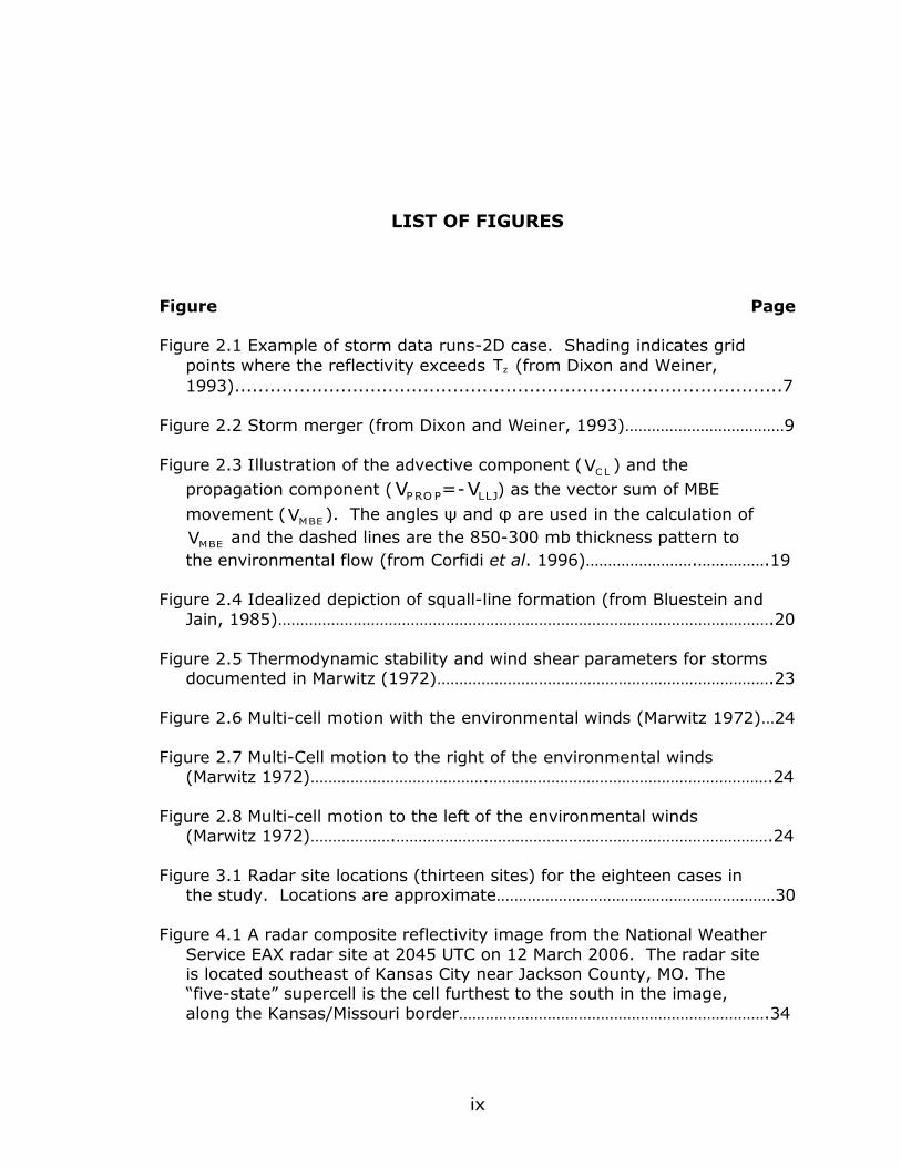
Figure Page Figure 2.1 Example of storm data runs-2D case. Shading indicates grid

points where the reflectivity exceeds Tz (from Dixon and Weiner,

1993).............................................................................................7

Figure 2.2 Storm merger (from Dixon and Weiner, 1993)………………………………9

Figure 2.3 Illustration of the advective component (VC L) and the

propagation component ( =VP RO P - LLJV ) as the vector sum of MBE

movement (VMBE). The angles ψ and φ are used in the calculation of

VMBE and the dashed lines are the 850-300 mb thickness pattern to

the environmental flow (from Corfidi et al. 1996)…………………….…………….19 Figure 2.4 Idealized depiction of squall-line formation (from Bluestein and

Jain, 1985)………………………………………………………………………………………………….20

Figure 2.5 Thermodynamic stability and wind shear parameters for storms documented in Marwitz (1972)………………………………………………………………….23

Figure 2.6 Multi-cell motion with the environmental winds (Marwitz 1972)…24

Figure 2.7 Multi-Cell motion to the right of the environmental winds (Marwitz 1972)………………………………….……………………………………………………….24

Figure 2.8 Multi-cell motion to the left of the environmental winds (Marwitz 1972)……………….………………………………………………………………………….24

Figure 3.1 Radar site locations (thirteen sites) for the eighteen cases in the study. Locations are approximate………………………………………………………30

Figure 4.1 A radar composite reflectivity image from the National Weather

Service EAX radar site at 2045 UTC on 12 March 2006. The radar site is located southeast of Kansas City near Jackson County, MO. The “five-state” supercell is the cell furthest to the south in the image,

along the Kansas/Missouri border…………………………………………………………….34

x

Figure 4.2 A radar composite reflectivity image from the National Weather Service NQA radar site at 2347 UTC on 2 April 2006. The supercell that

hit the town of Caruthersville, MO is indicated with the letter “A”. The radar site is located northeast of Memphis near Shelby County, TN…..….35


Service AMA radar site at 0032 UTC on 22 April 2007. The radar site is

located northwest of Amarillo near Potter County, TX……………….…………...36

Figure 4.4 A radar composite reflectivity image from the National Weather Service AMA radar at 0016 UTC on 29 March 2007. The arrow points

to the left-moving supercell………………………………………………………………………37


Service TWX radar site at 2135 UTC on 4 May 2003. The left-moving supercell in this case is indicated with the letter “B”. The radar site is located south of Topeka near Wabaunsee County, KS…………………………….38


Service NQA radar site at 1728 UTC on 7 April 2006……………….………………39

Figure 4.7 A radar composite reflectivity image from the National Weather Service LSX radar site at 0006 UTC on 20 July 2006. The radar site is located southwest on Saint Louis near Saint Charles County, MO….………40


Service LSX radar site at 1509 UTC on 21 July 2006……….……………………..41 Figure 4.9 A radar composite reflectivity image from the National Weather

Service UEX radar site at 0443 UTC on 9 July 2004. The radar site is located south of Hastings near Webster County, NE……………………………….42


Service FFC radar site at 0111 UTC on 3 May 2003. The radar site is

located southeast of Atlanta near Henry County, GA………………….……………43

Figure 4.11 A radar composite reflectivity image from the National Weather Service OHX radar site at 0415 UTC on 19 October 2004. The radar site is located northwest of Nashville near Robertson County, TN……………..….44


Service LSX radar site at 0244 UTC on 6 November 2005…………….……....45 Figure 4.13 A radar composite reflectivity image from the National Weather

Service FWS radar site at 2133 UTC on 6 August 2005. The radar site is located south of Fort Worth near Johnson County, TX…………………………….46

xi

Figure 4.14 A radar composite reflectivity image from the National Weather Service DGX radar site at 2030 UTC on 19 June 2006. The radar site is

located east of Jackson near Brandon in Rankin County, MS………………….47

Figure 4.15 A radar composite reflectivity image from the National Weather Service TBW radar site at 1829 UTC on 2 July 2006. The main outflow boundary is indicated with arrows. The radar site is located south of

Tampa in Hillsborough County, Florida……………….……………………………………48

Figure 4.16 A radar composite reflectivity image from the National Weather Service CCX radar site at 1659 UTC on 28 July 2006. The radar is located west of State College in Centre County, PA………………………………………………49


Service LWX radar site at 1948 UTC on 5 July 2004. The two cells mentioned in the case study description are indicated with arrows. The radar is located northwest of Sterling near Loudoun County, VA..………….50

Figure 5.1 Cell classification tree for the 53 cells in the study………………………53

Figure 5.2 A box-and-whisker plot of Mean-Layer Convective Available

Potential Energy (MLCAPE) values for cells tested in the study (n=53). Y-axis indicates MLCAPE values in J kg -1…………………………………………………57

Figure 5.3 A box-and-whisker plot of Vorticity Generation Parameter (VGP) values for cells tested in the study (n=53). Y-axis indicates

VGP values………………………………………………………………………………………………….58 Figure 5.4 A box-and-whisker plot of 0-3 kilometer Storm Relative

Helicity values for cells tested in the study (n=53). Y-axis indicates SRH values (m2s-2)…………………………………………………………………………………….60

Figure 5.5 A box-and-whisker plot of mean 0-6 kilometer wind shear values for cells tested in the study (n=53). Y-axis indicates wind

shear values (kts)………………………………………………………………………………………61

Figure 5.6 Illustration of velocities of cells tested in the study versus Isothermal winds. Y=X trendline indicates the equality of the

-20, -10, and 0°C isothermal wind velocities to supercell, linear, or

multicell velocities respectively…………………………………………………………………64

Figure 5.7 Same as Figure 5.14 for A) supercells, B) linear cells, and C) multicells……………………………………………………………………………………………….65

Figure 5.8 A comparison between the Actual Storm Direction of Motion(degrees) and -20°C isothermal wind (degrees) for cells tracked

in supercell cases. The solid line is a trendline of equality…….……………….67

xii

Figure 5.9 A comparison between the Actual Storm Direction of Motion (degrees) and -10°C isothermal wind (degrees) for cells tracked in

supercell cases. The solid line is a trendline of equality………………………….68

Figure 5.10 A comparison between the Actual Storm Direction of Motion (degrees) and 0°C isothermal wind (degrees) for cells tracked in

supercell cases. The solid line is a trendline of equality……………………….…69

Figure 5.11 A comparison between the Actual Storm Direction of Motion

(degrees) and -20°C isothermal wind (degrees) for cells tracked in linear cases. The solid line is a trendline of equality. Values over 360

degrees are cell motions near the 0/360 degree direction discriminator,

with 360 degrees added for continuity……………………………….…………………….71


linear cases. The solid line is a trendline of equality. Values over 360

degrees are cell motions near the 0/360 degree direction discriminator, with 360 degrees added for continuity……………………………………………………..72


(degrees) and 0°C isothermal wind (degrees) for cells tracked in linear cases. The solid line is a trendline of equality. Values over 360

degrees are cell motions near the 0/360 degree direction

discriminator, with 360 degrees added for continuity………………………….….73

Figure 5.14 A comparison between the Actual Storm Direction of Motion (degrees) and -20°C isothermal wind (degrees) for cells tracked in multicell cases. The solid line is a trendline of equality. Values over

360 degrees are cell motions near the 0/360 degree direction discriminator, with 360 degrees added for continuity………………………………74


(degrees) and-10°C isothermal wind (degrees) for cells tracked in

multicell cases. The solid line is a trendline of equality. Values over 360 degrees are cell motions near the 0/360 degree direction

discriminator, with 360 degrees added for continuity………………………….….75 Figure 5.16 A comparison between the Actual Storm Direction of Motion

(degrees) and 0°C isothermal wind (degrees) for cells tracked in multicell cases. The solid line is a trendline of equality………………….………76


(degrees) and -20°C isothermal wind (degrees) for cells tracked in

supercell cases. The red line is the y=x trendline, while the blue/black line is the line of best fit…………………………………………………………………………….79

xiii


linear cases. The red line is the y=x trendline, while the blue line is the line of best fit. Values over 360 degrees are cell motions near the

0/360 degree direction discriminator, with 360 degrees added for continuity……………………………………………………………………………………………………80

Figure 5.19: A comparison between the Actual Storm Direction of Motion (degrees) and 0°C isothermal wind (degrees) for cells tracked in

multicell cases. 360 degrees is added in some cases for continuity. The red line is the Y=X trendline, while the blue line is the line of best fit………………………………………………………………………………………………………..81

xiv

LIST OF TABLES

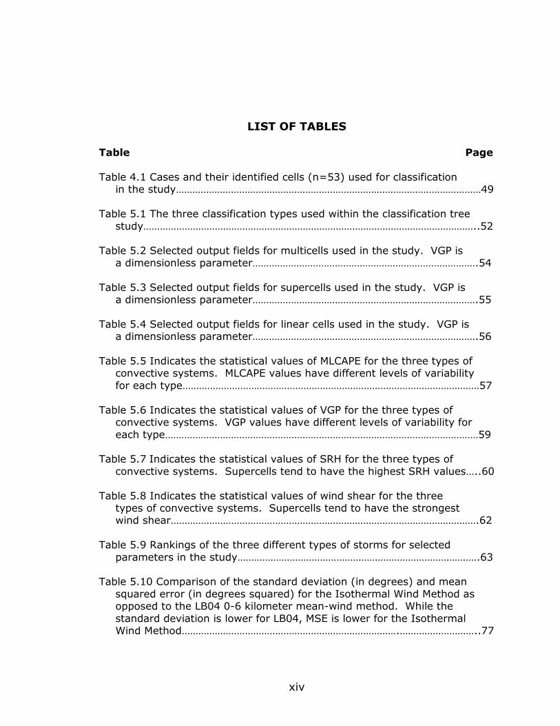
Table Page

Table 4.1 Cases and their identified cells (n=53) used for classification in the study…………………………………………………………………………………………………49

Table 5.1 The three classification types used within the classification tree

study…………………………………………………………………………………………………………..52 Table 5.2 Selected output fields for multicells used in the study. VGP is

a dimensionless parameter……………………………………………………………………….54

Table 5.3 Selected output fields for supercells used in the study. VGP is a dimensionless parameter……………………………………………………………………….55

Table 5.4 Selected output fields for linear cells used in the study. VGP is a dimensionless parameter……………………………………………………………………….56

Table 5.5 Indicates the statistical values of MLCAPE for the three types of

convective systems. MLCAPE values have different levels of variability

for each type………………………………………………………………………………………………57

Table 5.6 Indicates the statistical values of VGP for the three types of convective systems. VGP values have different levels of variability for

each type……………………………………………………………………………………………………59 Table 5.7 Indicates the statistical values of SRH for the three types of

convective systems. Supercells tend to have the highest SRH values…..60

Table 5.8 Indicates the statistical values of wind shear for the three types of convective systems. Supercells tend to have the strongest wind shear………………………………………………………………………………………………….62

Table 5.9 Rankings of the three different types of storms for selected

parameters in the study…………………………………………………………………………….63 Table 5.10 Comparison of the standard deviation (in degrees) and mean

squared error (in degrees squared) for the Isothermal Wind Method as opposed to the LB04 0-6 kilometer mean-wind method. While the

standard deviation is lower for LB04, MSE is lower for the Isothermal Wind Method…………………………………………………………………….………………………..77

xv

Table 5.11 Comparison of the standard deviation (in degrees) and mean squared error (in degrees squared) for the Isothermal Wind Method as

opposed to the C96 mean 850-300 mb wind method. Standard deviation and mean square error are smaller for the Isothermal Wind

Method…………………………………………………………………………………………………….….78 Table 5.12 Comparison of the standard deviation (in degrees) and mean

squared error (in degrees squared) for the Isothermal Wind Method as opposed to the M72 0-10 km mean wind method. The correlation

coefficient is more predictive with less error using the Isothermal Wind Method………………………………………………………………………………………………………..79

Table 5.13 Storm direction algorithms for the three types of storms……..…..80

Table 5.14 Range of isothermal levels (hPa) for selected isotherms in the study…………………………………………………………………………………………………………..83

Table 6.1 Cases used in the study………………………………………………………………….90

xvi

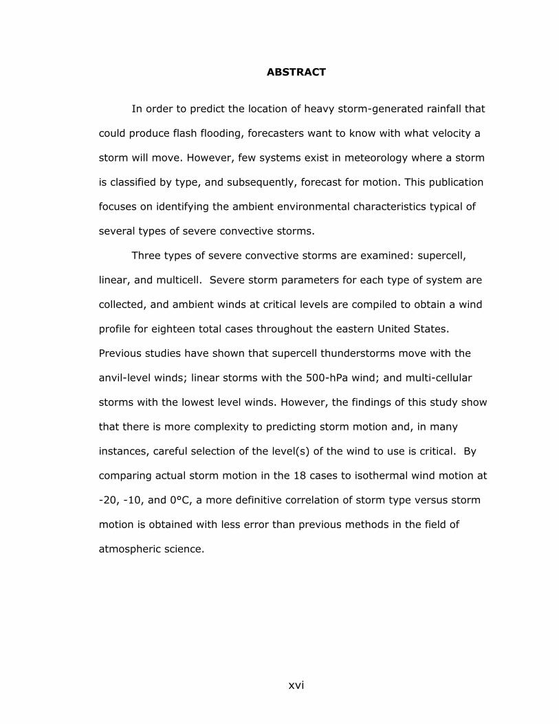
ABSTRACT

In order to predict the location of heavy storm-generated rainfall that

could produce flash flooding, forecasters want to know with what velocity a

storm will move. However, few systems exist in meteorology where a storm

is classified by type, and subsequently, forecast for motion. This publication

focuses on identifying the ambient environmental characteristics typical of

several types of severe convective storms.

Three types of severe convective storms are examined: supercell,

linear, and multicell. Severe storm parameters for each type of system are

collected, and ambient winds at critical levels are compiled to obtain a wind

profile for eighteen total cases throughout the eastern United States.

Previous studies have shown that supercell thunderstorms move with the

anvil-level winds; linear storms with the 500-hPa wind; and multi-cellular

storms with the lowest level winds. However, the findings of this study show

that there is more complexity to predicting storm motion and, in many

instances, careful selection of the level(s) of the wind to use is critical. By

comparing actual storm motion in the 18 cases to isothermal wind motion at

-20, -10, and 0°C, a more definitive correlation of storm type versus storm

motion is obtained with less error than previous methods in the field of

atmospheric science.

1

Chapter 1

Introduction

In the field of atmospheric science, storm motion has been a

topic defined by a vast amount of research from numerous agencies.

However, associating conclusively storm motion with storm type has

shown to be one of the least researched topics in the field. Two of the

most widely used nowcasting programs used in atmospheric science

(the Spectral Prognosis scheme, or S-PROG, and Warning Decision and

Support System-Integrated Information, or WDSS-II) intuitively use

storm motion to make nowcasts of precipitation and storm intensity.

These programs could be further enhanced by classifying severe

convective storms by type and subsequently forecasting the motion of

the storms from this information---along with existing environmental

conditions.

Being able to determine whether storm type is a determining

factor in storm motion has several practical results. Forecasters can

warn the public in specific areas about certain severe weather threats,

giving those warned more time to prepare for potential hazards.

Second, applications to industry/business are also affected by storm

motion, as the livelihood of many occupations are determined by the

amount, intensity, and location of rain, hail, tornadoes, and other

2

weather phenomena. Third, storm type forecasts of storm motion can

be used to provide another critical measure of uncertainty, as existing

environmental conditions can be documented and “databased” to give

forecasters a better idea of the growth, decay, merging, or splitting of

storms in certain environmental conditions.

1.1 Statement of Thesis

The purpose of this study is to determine if storm motion is an

advantageous method of classifying storm type. This will help

forecasters make specialized nowcasts of convective weather

conditions in a given area. By looking at three different types of cases

with a statistical classifier, we can determine if the classifier can

delineate types of storms based on their conditions which will be

explored in the study.

Forecasters presently notify the public of severe weather

conditions by noting current surface observations and using

extrapolations of cell motion through various modes of radar imagery.

Programs that forecasters currently use to track severe storms have

no regard for storm type or environmental situations. These programs

generally also use “standard” levels (850 mb, 700 mb, etc.) which may

not be representative of the actual cloud-layer or vertical structure of

every storm, yet are convenient for access. By knowing which

3

conditions are conducive to certain types of storms using information

related to isothermal-level winds, forecasters will be aided in

determining the future motion of those storms, and thus, give a better

forecast of severe weather conditions for a given area. The objectives

of this study are to:

Determine the pre-existing meteorological conditions

associated with three different types of severe convective

storm systems (supercell, linear, multi-cell).

Determine if the statistical classifier can delineate these

types based on said meteorological conditions, and finally;

Determine if storm motion can be more accurately

predicted by the success of the statistical classifier in

correctly indicating the convective mode of storms at

storm genesis.

The main hypothesis to be tested in the study is that pre-

existing dynamic and thermodynamic conditions (convective

available potential energy, shear, etc.) will be different for each

convective mode, and will therefore affect the motion of the storms

in those modes. A second hypothesis is since the convective modes

will have different environmental conditions, the statistical classifier

will be able to note these differences and successfully identify

4

supercell, linear, and multi-cell convective systems. The success of

the hypotheses will generate more accurate storm motion forecasts

by the classification of storm type.

5

Chapter 2

Literature Review

Determining whether storm type is an important criterion for

storm motion has far-reaching effects. Not only is it difficult

operationally to delineate between and correctly predict storm type

and motion, it is also difficult from an artificial intelligence standpoint.

The implications of an erroneous nowcast of storm motion on the time

scale of 0-60 minutes can be the difference between a forecast of

tranquil weather or potentially severe/damaging weather conditions,

with arising complications for emergency management personnel,

government officials, and the public alike. For a comprehensive

examination of relevant literature of the topic, this chapter will

examine the research conducted thus far concerning the general

motion characteristics of storms. Next, the specific motion

characteristics of three types of storms; supercell, squall-line, and

discrete multicell will be explored.

2.1 Forecasting Storm Motion

A great amount of time and effort has been invested to predict

storm motion. In order for forecasters to predict storm motion, one

must identify the location of the storm cells at initiation. The

6

Thunderstorm Identification, Tracking, Analysis, and Nowcasting

system, or TITAN as explained in Dixon and Weiner (1993) gives a

storm definition as a contiguous region that exhibits reflectivities

above a given threshold (Tz ), and the volume which exceeds a

threshold (Tv ). For individual convective cells, Tz equals 40-50 dBZ,

while Tz for convective storms equals 30-40 dBZ (these thresholds can

be adjusted by the user/forecaster). To identify storms, contiguous

regions above Tz were needed. This was done by 1) identifying

contiguous sequences of points (referred to in Dixon and Weiner

(1993) as runs) in one of the two-dimensional principal directions (x or

y direction) for which the reflectivity exceeds Tz and 2) group runs

that are adjacent. This process is summarized in Figure 2.1:

Figure 2.1: Example of storm data runs-2D case. Shading indicates grid

points where the reflectivity exceeds Tz (from Dixon and Weiner, 1993).

The question then turns from storm identification to storm

tracking. TITAN searches for the optimum set of storm paths by the

following method, which will hereafter be referred to as the “optimal

7

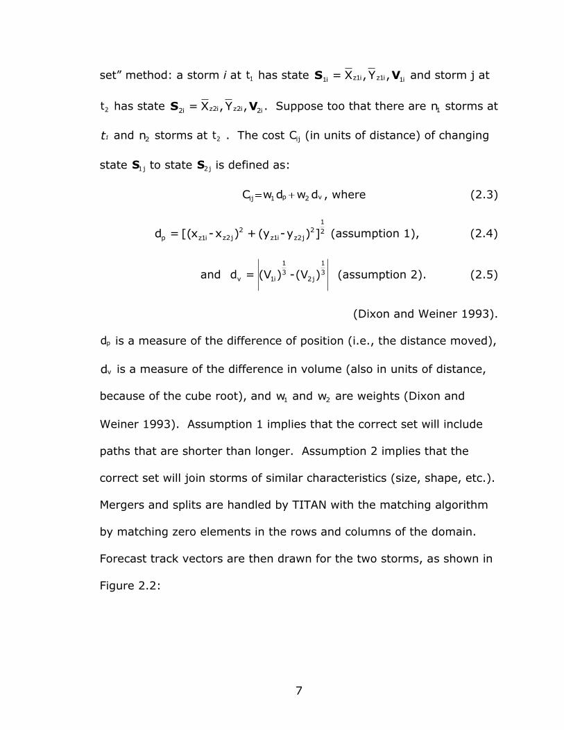
set” method: a storm i at t1 has state i1i1zi1zi1 ,Y,X= VS and storm j at

t2 has state i2i2zi2zi2 ,Y,X= VS . Suppose too that there are n1 storms at

t1 and n2 storms at t2 . The cost Cij (in units of distance) of changing

state S1j to state S2 j is defined as:

Cij w1dp w2 dv , where (2.3)

i1zp x[(=d - i1z2

j2z y(+)x - 2

1

2j2z ])y (assumption 1), (2.4)

and 3

1

i1v )V(=d - 3

1

j2 )V( (assumption 2). (2.5)

(Dixon and Weiner 1993).

dp is a measure of the difference of position (i.e., the distance moved),

dv is a measure of the difference in volume (also in units of distance,

because of the cube root), and w1 and w2 are weights (Dixon and

Weiner 1993). Assumption 1 implies that the correct set will include

paths that are shorter than longer. Assumption 2 implies that the

correct set will join storms of similar characteristics (size, shape, etc.).

Mergers and splits are handled by TITAN with the matching algorithm

by matching zero elements in the rows and columns of the domain.

Forecast track vectors are then drawn for the two storms, as shown in

Figure 2.2:

8

Figure 2.2: Storm merger (from Dixon and Weiner, 1993).

The following assumptions were made by Dixon and Weiner

(1993) to formulate the storm forecast algorithm:

A storm tends to move along a straight line.

Storm growth or decay follows a linear trend.

Random departures from the above behavior occur.

The forecast ellipse assumes that the orientation of the storm remains

constant---an assumption later refined in future nowcasting systems.

The WSR-88D SCIT (Storm Cell Identification and Tracking)

algorithm as described in Johnson et al. (1998) was developed to

identify, characterize, track, and forecast the short-term movement of

storm cells identified in three dimensions. MR-SCIT, a centroid-based

cell identification and diagnosis algorithm described by Lakshmanan et

al. (2002), worked by overlapping the 2D features of the WSR-88D

SCIT system and running them on multiple sites to create a 3D system

9

of overlapped data sets from these radars. This allowed a more

complete vertical analysis of storms where data was poor. The

information from multiple radars was used to identify and track

individual storm cells. Multiple radar data was detailed by Lynn and

Lakshmanan (2002), in terms of “virtual volume” scans, with the latest

elevation scan of data replacing the one from a previous volume scan

(Lakshmanan et al. 2002).

Vertical and time association was performed at five-minute

intervals which enables updating of the multiple-radar data. The

virtual volumes containing data from the latest radar scan were

combined to produce a vertical cross-section representing storm cells.

Cell-based information such as POSH (Probability of Significant Hail)

and hail size were also diagnosed by Lakshmanan et al. (2002) using

the 2D to 3D combined multiple radar data system, as well as storm

environment data from mesoscale models. Storm cells were tracked in

time, and 30-minute nowcasts were made.

Three-dimensional storm identification begins with one-

dimensional data processing to identify storm segments in the radial

reflectivity data. A storm segment was saved in the Johnson et al.

(1998) study if its radial length was greater than a preset threshold,

usually around 1.9 km. WDSS then repeated the process using seven

different reflectivity thresholds (60, 55, 50, 45, 40, 35, and 30 dBZ).

10

After the last radial of the elevation scan was analyzed, individual

storm segments were combined into 2D storm components based on

their proximity to one another (Johnson et al. 1998). This proximity is

based on a 1.5 degree or closer azimuthal location and overlap in

range of usually 2 kilometers. It was defined in the Johnson et al.

(1998) study that storms must have two components and an area

larger than 10 square kilometers. After 2D scans are made, 3D storm

cells were made by merging two or more 2D storm components at

different elevation angles. Scans were then made in an eliminatory

process at 5, 7.5 and 10 km to see if two storm centroids were within

these distances. The result is a 2D and 3D “snapshot” of a storm cell

centroid; the storm cells are then ranked by their vertically integrated

liquid water value (VIL) (Johnson et al. 1998). This method, however,

has some drawbacks including poor temporal resolution (5-minute

updates), and the fact that the algorithm uses data based from

individual radars. Some attempts are being made to resolve these

issues, including creating polar grids using a virtual volume value each

time the radar scans, and a second method, computing VIL on multi-

radar grids using 1 km grid spacing (Lakshmanan et al. 2002).

Storm cells identified in two consecutive volume scans are

associated temporally to determine the cell track (Johnson et al.

1998). If the time difference is greater than 20 minutes, the second

11

scan is not attempted. This can happen due to malfunctions in the

radar or interrupted communications. Using the centroid locations

from the previous volume scan, a “guess” at the next location is

created with the next volume scan (Johnson et al. 1998). To “guess”,

WDSS uses the storm motion vector of the previous volume scan or a

default motion vector if no previous one is detected. The motion

vector of the storm is determined by using an average of all the storm

cells’ motion vectors in the interface, or user input of the average 0-6-

km wind speed and direction vectors of the cell. Next, the distance

between the centroid of each cell and the “guess” of the next

successive volume scan is calculated; if the distance is less than the

threshold value, the distance between the new cell and all possible

matches are determined (Johnson et al. 1998). The match with the

smallest distance is considered the time-association of the detected

cell. The motion vector is then calculated for the new cell by using a

linear least squares fit of the storms’ current and up to 10 previous

locations (see Figure 2). Each of the locations is given equal weight

(Johnson et al. 1998). Once the tracking process is completed, data is

tabulated for up to 10 previous volume scans.

Fox and Wilson (2005) and Jankowski (2006) found that the

WSR-88D SCIT system works well with storms moving along linear

paths. However, precipitation systems more often than not move in a

12

non-linear fashion, and the SCIT system provides no measurement of

uncertainty within the forecast. Fox et al. (2007) concluded that the

forecast motion is dependent upon the choice of precipitation area that

is delineated. Micheas et al. (2007) used idealized elliptical cells to

decompose the error contributions of various attributes such as

orientation, size, and translation in a Procrustes verification scheme

useful for a more robust verification solution.

By implementing a user-defined threshold of size and intensity

for the object, the scheme identifies forecast objects (i.e. storm cells)

of reflectivity. The cells in the forecast field are then matched to the

cells in the observed field. The information on the error based on size,

translation, and rotation are combined with error based on intensity

values via a penalty function. The Micheas et al. (2007) forecast

scheme begins shape analysis once matching is accomplished. The

forecast object is overlaid onto its corresponding observed field and a

fit is performed using the equation:

z^j

c^ jk r^ jk ei ^jk

zkj . (2.1)

Equation 2.1 is known as the full Procrustes fit, the superposition

of zkj onto z

j where the first component c is the translation term, r is

the dilation term and is the rotational component. Micheas et al.

(2007) used these terms to incorporate the residual sum of squares

(RSS) term in the penalty function:

13

D RSSk SSavgk

SSmink

SSmaxk (2.2)

The other components in the penalty function are the errors

based on intensity differences between the forecast and observed

object summed for the entire domain, thus, the lower the penalty, the

better the forecast solution. It is interesting to note that case 14 in

the Lack et al. (2007) study, a likely linear case, performed the best

with the lowest penalty function.

2.2 Storm Type Classification

As the Micheas et al. (2007) verification scheme assesses the

shape of the storm cell Lack et al. (2007) developed this in

combination with near-storm environment parameters to objectively

identify storm type using a decision tree. An automated rainfall

system classification procedure with attributes that explore the

characterization of the changing aspects of rainfall patterns can be an

important technique to minimize the error of determining storm type

(Baldwin et al. 2005). This was tested in recent work by comparing

the results of automated various cluster analysis with a human expert

classification of three storm types: linear, cellular, and stratiform, as

well as two classes: convective and non-convective (Baldwin et al.

2005). Rainfall systems were defined as contiguous areas of

precipitation, and the distribution of the random sample of objects was

14

scrutinized with respect to summary statistics to ensure a sample

representative of the population.

2.3 Forecasting Supercell Motion

Supercells are defined similar to Moller et al. (1994): convective

storms with mesocyclones or mesoanticyclones. Pinto et al. (2007)

defined supercells as storms with areal coverage greater than 50

square kilometers and a peak reflectivity greater than 50 dBZ.

Forecasters have spent the latter half of the twentieth century trying

to obtain a better understanding of supercell propagation in relation to

winds at multiple levels.

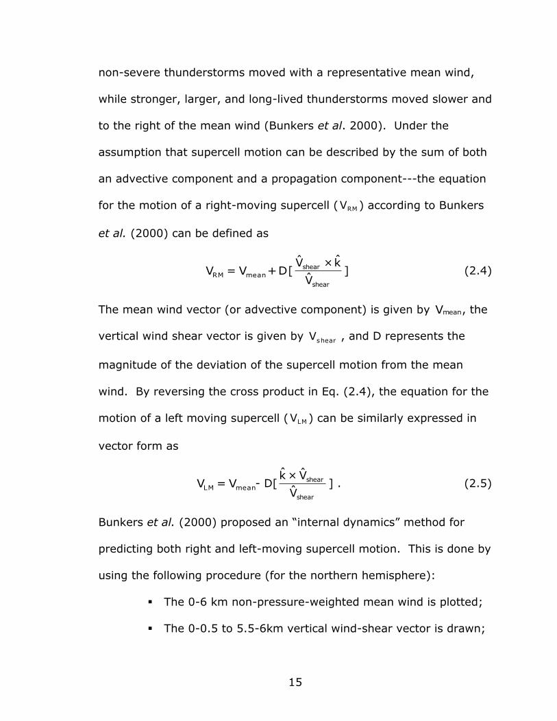
Two components are largely responsible for supercell motion as

defined by Bunkers et al. (2000) --- (i) advection of the storm by a

representative mean wind, and (ii) propagation away from the mean

wind either toward the right or to the left of the vertical wind shear---

due to internal supercell dynamics. Knowledge of supercell motion has

become widely known recently as anvil-level storm-relative flow has

been used to discriminate among types of supercells (Rasmussen and

Straka 1998). Thus, reliable prediction of supercell motion prior to

supercell development is one key to improving severe weather

forecasts. Extensive research was conducted in the mid-20th century

pertaining to thunderstorm motion. It was generally observed that

15

non-severe thunderstorms moved with a representative mean wind,

while stronger, larger, and long-lived thunderstorms moved slower and

to the right of the mean wind (Bunkers et al. 2000). Under the

assumption that supercell motion can be described by the sum of both

an advective component and a propagation component---the equation

for the motion of a right-moving supercell (VRM ) according to Bunkers

et al. (2000) can be defined as

D+V=V meanRM [shear

shear

V̂

k̂×V̂] (2.4)

The mean wind vector (or advective component) is given by Vmean, the

vertical wind shear vector is given by Vshear , and D represents the

magnitude of the deviation of the supercell motion from the mean

wind. By reversing the cross product in Eq. (2.4), the equation for the

motion of a left moving supercell (VLM ) can be similarly expressed in

vector form as

meanLM V=V - D[shear

shear

V̂

V̂×k̂] . (2.5)

Bunkers et al. (2000) proposed an “internal dynamics” method for

predicting both right and left-moving supercell motion. This is done by

using the following procedure (for the northern hemisphere):

The 0-6 km non-pressure-weighted mean wind is plotted;

The 0-0.5 to 5.5-6km vertical wind-shear vector is drawn;

16

cA line that both is orthogonal to the shear and passes

through the mean wind is drawn;

The right-moving supercell 7.5 m s 1 from the mean wind

along the orthogonal line to the right of the vertical wind

shear is located, and

The left-moving supercell 7.5 m s 1 from the mean wind

along the orthogonal line to the left of the vertical wind

shear is located.

From Bunkers et al. (2000)

Left moving supercells have been observed, most notably by

Lindsey and Bunkers (2004), contrary to most observed convective

systems. Lindsey and Bunkers examined the differences between left-

movers and their counterparts with respect to evolution, anvil

orientation, and interaction with right-moving supercells, inferring that

“…the left-moving supercell of velocity 13 m/s faster than the right-

moving supercell in the case, when it interacted with it, disrupted its

rotation.” Thus, left-moving supercells involved in merger scenarios

may have a disorganizing effect on their right-moving counterparts.

This is consistent with earlier research on the effects of storm mergers

on tornadogenesis (Finley et al. 2001).

17

The left mover in the Lindsey and Bunkers (2004) case affected

its right counterpart thermodynamically and dynamically in numerous

ways:

“…since the left mover progressed through the inflow of

the right mover, it likely altered both the thermodynamics of the inflow and the ambient wind field into which the

right mover progressed. The left mover intersected the forward flank of the right mover, so the anticyclonic

rotating updraft of the left mover may have destructively interfered with the cyclonic rotating updraft of the right

mover, resulting in less net rotation and therefore storm disorganization.”

Anvil orientations were calculated for 479 right-moving supercells and

compared to a theoretical left-moving supercell similar to the one

looked at in the specific case study by Lindsey and Bunkers (2004).

The median difference of anvil orientation for left and right-moving

supercells was 54° (Lindsey and Bunkers 2004).

2.4 Forecasting Squall-line Motion

The squall line has been defined loosely as a linearly oriented

mesoscale convective system (Maddox, 1980; Bluestein and Jain

1985), hereafter known as MCS. Corfidi et al. (1996) defined MCS

motion as a vector sum of an advective component, and a propagation

component, stated as the Corfidi vector. Thus, Corfidi et al. (1996)

modeled MCS core motion as the vector sum of a vector representing

cell advection by the mean-cloud-layer wind and a vector representing

18

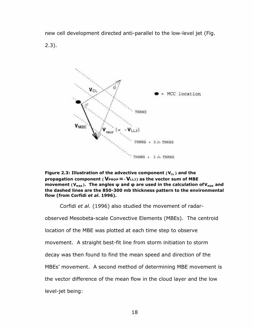
new cell development directed anti-parallel to the low-level jet (Fig.

2.3).

Figure 2.3: Illustration of the advective component (VCL ) and the

propagation component ( =VPROP - LLJV ) as the vector sum of MBE

movement (VMBE). The angles ψ and φ are used in the calculation ofVMBE and

the dashed lines are the 850-300 mb thickness pattern to the environmental

flow (from Corfidi et al. 1996).

Corfidi et al. (1996) also studied the movement of radar-

observed Mesobeta-scale Convective Elements (MBEs). The centroid

location of the MBE was plotted at each time step to observe

movement. A straight best-fit line from storm initiation to storm

decay was then found to find the mean speed and direction of the

MBEs’ movement. A second method of determining MBE movement is

the vector difference of the mean flow in the cloud layer and the low

level-jet being:

19

C LMBE V=V - LLJV . (2.6)

The hypothesis in Corfidi et al. (1996) was correct; the advective

component is dictated by the mean cloud layer and the propagation

component has a tendency to propagate towards the low-level jet.

This was suitable for operational use and provided insight in

forecasting MCS motion (Jankowski, 2006). This study will look at the

importance of motion vector differencing with storm type.

Squall lines can be broken down further into four distinct

categories: broken line, back-building, broken areal, and embedded

areal (Fig 2.4).

Figure 2.4: Idealized depiction of squall-line formation (from Bluestein and

Jain, 1985).

20

Bluestein and Jain (1985) defined squall line motion as oriented

along the mean wind in the lowest 1 km, at a large angle to the wind

in the lowest part of the middle troposphere, and at an angle of 30-

40° from the shear somewhere in the upper troposphere. Therefore,

squall lines fall into the steering category proposed by Moncrieff

(1978); each type has a mean steering level (MSL) with respect to line

motion around 6 or 7 km above the surface. Cells tend to move along

the line, with a little component against line motion (fig. 2.4):

(Bluestein and Jain 1985). Charba and Sasaki (1971) found that linear

storm systems displace towards the right of the mean wind even

though individual cells may move in the direction of the ambient

upper-level winds. This displacement occurs as new cells develop up-

stream from existing cells towards the right-flank, low-level inflowing

current (Charba and Sasaki 1971), thus occurring when winds veer

with height.

2.5 Forecasting Multi-Cell Motion

The National Weather Service (NWS) has defined multicell

thunderstorms as clusters of at least 2-4 short-lived cells. Each cell

generates a cold air outflow; these individual outflows combine to form

a large gust front. Convergence along the gust front allows new

storms to develop; the cells move roughly with the mean wind at first,

21

but then deviate significantly from the mean wind due to new cell

development along the gust front. Fovell and Tan (1996) defined

multicells as a family of cells within a cross section of the idealized

squall-line, each representing a different stage in the life cycle.

Research pertaining to multi-cellular thunderstorms has been

conducted for decades, with Browning and Ludham (1960) existing as

the first significant study of storms of a multi-cellular nature.

Browning and Ludham (1960) worked with a series of aligned cells

near Wokingham, England in which new cells periodically developed on

the right flank, moved with the storm complex, and dissipated on the

left flank. This form of discrete propagation caused deviant motion

towards the right flank. Chisholm (1966) analyzed two multi-cell

storms in Alberta, which deviated towards the right flank by discrete

propagation while individual cells within the storm complex moved in

the direction of the environmental winds. The environmental

conditions for the storms are noted here in figure 2.5:

22

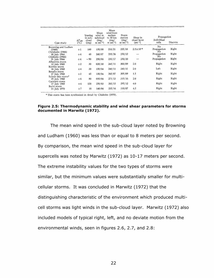
Figure 2.5: Thermodynamic stability and wind shear parameters for storms

documented in Marwitz (1972).

The mean wind speed in the sub-cloud layer noted by Browning

and Ludham (1960) was less than or equal to 8 meters per second.

By comparison, the mean wind speed in the sub-cloud layer for

supercells was noted by Marwitz (1972) as 10-17 meters per second.

The extreme instability values for the two types of storms were

similar, but the minimum values were substantially smaller for multi-

cellular storms. It was concluded in Marwitz (1972) that the

distinguishing characteristic of the environment which produced multi-

cell storms was light winds in the sub-cloud layer. Marwitz (1972) also

included models of typical right, left, and no deviate motion from the

environmental winds, seen in figures 2.6, 2.7, and 2.8:

23

Figure 2.6: Multi-cell motion with the environmental winds (Marwitz 1972).

Figure 2.7: Multi-Cell motion to the right of the environmental winds

(Marwitz 1972).

Figure 2.8: Multi-cell motion to the left of the environmental winds (Marwitz

1972).

By examining pertinent research, one can conclude that several

factors will determine the ultimate motion of a severe convective

storm. By documenting and classifying individual cells, one can infer

the general track of the cells, as well as evaluate the overall

effectiveness of nowcasting systems in forecasting those cells’

motions. Thus, with a better classification and evaluation system for

24

storm type, one can better infer storm motion, improving forecasts

and reducing error.

25

Chapter 3

Methodology

3.1 Study Focus

Storm motion can be affected by several factors such as the

relative timeframe of the storm in its life cycle, splitting, merging,

propagation into stable or unstable air masses, and the relative

location of the cell in the parent storm system. For this study, storm

motion will be measured in meteorological coordinates (0° indicates

from the north, 90° indicates from the east, etc.) unless otherwise

stated. This study will attempt to determine if storm motion can be

more accurately predicted by classifying storm type at genesis and

knowing the meteorological conditions associated with those types.

3.1.1 Area of Study

Three different geographical regions of the United States exist

as the area of focus for this study. Eighteen (18) storm systems are

contained in the three regions classified as eastern, Midwestern, and

southern. The eastern region contains cases in the states of

Pennsylvania (PA) and Virginia (VA). The Midwestern region contains

cases from Missouri (MO), Kansas (KS) and Nebraska (NE), while the

southern region contains cases from Tennessee (TN), Texas (TX),

26

Georgia (GA), Mississippi (MS), and Florida (FL). Three regions are

used to apply information learned in the study to different sections of

the country. The eighteen cases are broken down into three

categories defined by the convective mode of storms in the cases:

supercell, linear, and multi-cell. Within the events, ambient wind

profiles/conditions are noted, and individual cells are identified and

tracked for motion.

3.1.2 Selection of Storm Cells

The first category of case studies consisted of events with

supercell characteristics, in which a selection procedure needed to be

utilized. Storm cells in this category were picked based on their size.

The statistical classifier used in the study allowed a user-defined

threshold for the objects, in which supercells smaller than 500

2km (Lack 2007) in any case were discarded.

Storm cells within this category were selected also based on a

user-defined threshold of reflectivity, similar to the Pinto et al. (2007)

peak reflectivity threshold of 50 dBZ. If the cell on four consecutive

scans (~20 min) maintained a peak reflectivity of higher than 50 dBZ,

it was included in the study. The use of four scans was determined

based on a modified Bunkers et al. (2000) definition for two reasons:

first, most supercells last shorter than 2 hours; some supercells

27

(rarely) last less than 10 minutes, and, four scans also implies that

storm tracking is possible, and above all else, reliable.

The second category of case studies consisted of events with

squall-line characteristics, in which individual convective cells within

the squall-line were tracked for motion as well as the squall-line itself.

Squall-lines in the category were selected based on the Bluestein and

Jain (1985) definition of related or similar echoes that form a pattern

exhibiting a length-to-width ratio of at least 5:1, greater than or equal

to 50 km long, and persisting for longer than 15 minutes (or 3 volume

scans). These features were chosen because of their consideration to

be mesoscale as well as their increased probability of containing cells

with lifecycles relevant to the study as described above.

The third category of case studies consisted of events with multi-

cell characteristics, in which cells at different points in their life-cycles

are tracked for motion. Multi-cells in this category were selected

based on their life cycle of less than 1 hour as described by Fovell and

Tan (1996) and their user-defined size (roughly 50-100 2km ). Cells in

this category were also selected based on a user-defined threshold of

reflectivity greater than 30 dBZ as most thunderstorms with multi-cell

characteristics rarely produce heavy rainfall (in excess of 50 dBZ) for

more than 15 minutes. If the cell maintained a peak reflectivity

28

greater than 30 dBZ for more than 3 consecutive volume scans, it was

included in the study.

3.2 Data

Radar data for each case were collected from the National

Climate and Data Center (NCDC) in the form of level II NEXRAD data

and processed through radar display software called the Warning

Decision Support System-Integrated Information (WDSS-II). WDSS-II

utilizes a National Severe Storms Laboratory (NSSL) algorithm similar

to Johnson et al. (1998) which identifies an individual storm’s location,

movement, and other characteristics within a cell table.

Storm environment data were collected from the NCDC in the

form of Rapid Update Cycle-252 (RUC-252) 20 km resolution data for

all eighteen cases. The data were compiled in the “grib” file format, in

which WDSS-II converts the grib files to text files using the

“GribtoNetCDF” command. Boundaries were specified in the

GribtoNetCDF command to match the radar Cartesian 256 X 256 km

grid, allowing the model data for each case to be overlaid on grids of

radar reflectivity.

29

3.3 Procedure

To track cells for motion and speed a number of steps had to be

completed. Radar data were analyzed from the following National

Weather Service (NWS) radar sites (Fig. 3.1): Kansas City, MO (EAX),

Memphis, TN (NQA), Amarillo, TX (AMA), Saint Louis, MO (LSX),

Hastings, NE (UEX), Atlanta, GA (FFC), Nashville, TN (OHX), Fort

Worth, TX (FWS), Jackson, MS (JAN), Tampa Bay, FL (TBW), State

College, PA (CCX), Sterling, VA (LWX), and Columbus Air Force Base,

MS (GWX).

Figure 3.1: Radar site locations (thirteen sites) for the eighteen cases in the

study. Locations are approximate.

Storm motion and velocity was tabulated for each cell in each

case by averaging the 5-minute SCIT centroid motion values (in

30

WDSS-II) during the life of the cell. Near-storm environments are

derived from model data ingested into WDSS-II. In the specific case

of RUC-model isothermal winds, the values were taken from the

specific 20 X 20 km “center” of the cell. From the model data several

parameters were tabulated for each cell which included height of 0, -

10, and -20°C isotherms; mean wind speed from surface to 6

kilometers (measured in knots); storm motion (direction measured in

degrees, speed measured in knots); shear from 0-6 kilometers

(measured in m -1-1 km s ); propagation (left or right in the case of

supercells and multicells, and direction in the linear cases); mean-

layer convective available potential energy (MLCAPE; measured in J

1kg ), 0-3-km storm relative helicity (SRH; measured in 22 s m ), the u

and v-wind components at the 0, -10, and -20°C isotherms (measured

in knots), and the dimensionless Vorticity Generation Parameter

(VGP), which is defined in Rasmussen and Blanchard (1998) as

VGP= ][S(CAPE) 2

1

(3.1)

where (S) is the mean shear in the column. These parameters were

chosen from the Marwitz (1972) multicell study and the Lack et al.

(2007) cell classification study for their usefulness for all storm types.

Comparisons of the parameters were then made between cases and

similarities/differences were noted.

31

The cases were subsequently analyzed with a cell identification

script in MATLAB with the previous parameter information included.

The “numberID_simp.m” file identifies the individual cell to be

analyzed, while the “identifycells.m” file lists cells that match the size

criteria in a “finalarray” function. The script also produces images of

each convective system for easy reference. Scripts for the files are

included in the appendix. With these calculations, the success of the

classifier in identifying convective systems of different types was

analyzed.

The 0, -10, and -20°C isotherms, as well as their u and v-wind

components, were chosen because of their proximity to the cloud layer

steering winds (Marwitz 1972) as well as their variability in height in

different cases, and subsequent, lack of upper and lower height

boundaries. The mean wind speed from the surface to 6 kilometers

was chosen as a parameter to compare with the speed of propagation

of the individual convective system. The shear from 0-6 kilometers

was chosen to note pre-existing environmental conditions prior to

storm genesis and to note trends among storms of different types.

Propagation, MLCAPE, 0-3 kilometer SRH, and VGP were noted for the

same reason.

32

Chapter 4

Case Studies

Eighteen storm events were selected for this study from a range

of geographical regions within the continental United States. Storm

events were divided into three different categories: supercell, squall-

line, and multi-cell with six events in each category. The basis for the

categories was the appearance of the storms and the orientation of the

storm systems (discrete, linear, or clustered). The following sections

will describe these events in detail.

4.1 Supercell Events

4.1.1 12 March 2006: Pleasant Hill, MO region

The National Weather Service (NWS) WSR-88D radar located in

Pleasant Hill, MO recorded a supercell event during the period 1900

UTC 12 March 2006 to 2230 UTC 12 March 2006. Two supercells are

of note in this event: the first being the “five-state” supercell, which

tracked across northeastern Oklahoma, Kansas, Missouri, Illinois, and

northwestern Indiana before finally dissipating 17.5 hr after genesis.

The second supercell formed just to the north of the five state

supercell and eventually merged with it near the Missouri-Illinois

33

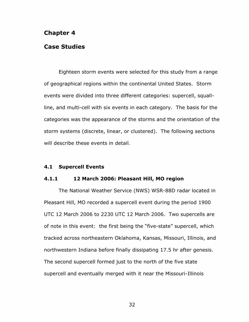
border. Figure 4.1 shows four distinct supercells moving northeast

through Missouri on 12 March 2006 that produced several tornadoes.

Figure 4.1: A radar composite reflectivity image from the National Weather

Service EAX radar site at 2045 UTC on 12 March 2006. The radar site is

located southeast of Kansas City near Jackson County, MO. The “five-state”

supercell is the cell furthest to the south in the image, along the

Kansas/Missouri border.

4.1.2 2-3 April 2006: Memphis, TN region

This event occurred over two separate regions on 2 April 2006 as

discrete supercells merged and formed a squall line that stretched

from western Illinois south through eastern and southeastern Missouri.

In this case, a discrete supercell on the southwestern flank of the

squall line was responsible for an F2 tornado that hit the town of

Caruthersville, MO, just to the north of the NQA radar site (around

34

2350 UTC 2 April 2006). This study will focus on the period of 2130

UTC 2 April to 0200 UTC 3 April. Figure 4.2 shows four supercells

moving east through sections of Missouri, Arkansas, and Tennessee.

Figure 4.2: A radar volume scan from the National Weather Service NQA

radar site at 2347 UTC on 2 April 2006. The supercell that hit the town of

Caruthersville, MO is indicated with the letter “A”. The radar site is located

northeast of Memphis near Shelby County, TN.

4.1.3 21-22 April 2007: Amarillo, TX region

An upper-level low pressure system which moved out of the

intermountain west into the Great Plains was responsible for this event

which occurred near Amarillo, TX from 2200 UTC 21 April 2007 to

0300 UTC 22 April 2007. Numerous supercells on the southwestern

flank of an east-moving squall-line are portrayed on the AMA radar

image (see figure 4.3). Maturing over the city, the supercells

A

35

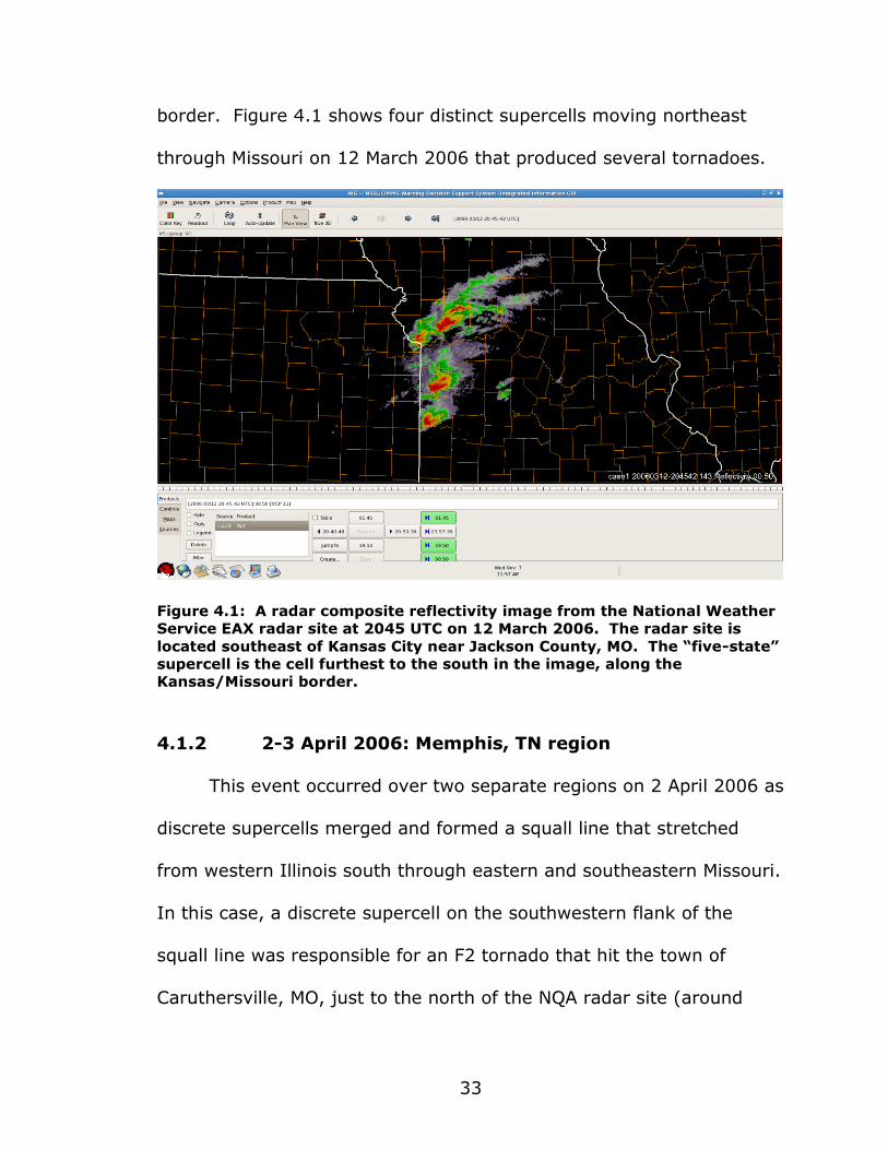
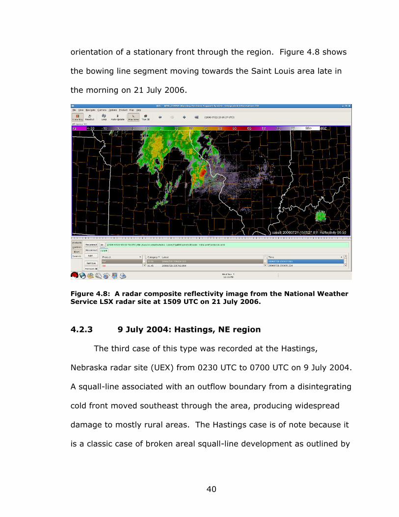
produced several reports of property damage. Figure 4.3 shows

numerous supercells tracking to the north-northeast towards the city

of Amarillo.


Service AMA radar site at 0032 UTC on 22 April 2007. The radar site is

located northwest of Amarillo near Potter County, TX.

4.1.4 28-29 March 2007: Amarillo, TX region

The AMA radar located in Amarillo, TX observed a left-moving

supercell of note from 2100 UTC 28 March 2007 to 0330 UTC 29 March

2007. The storm-relative motion of the supercell was north-

northwest; it generated from another supercell which was moving to

the northeast. The left-moving supercell, however, proved to be much

weaker than the parent supercell which produced numerous tornado

reports in the panhandle of Texas. Figure 4.4 shows five supercells

36

moving through the panhandle of Texas that produced numerous

confirmed tornadoes.


Service AMA radar site at 0016 UTC on 29 March 2007. The arrow points to

the left-moving supercell.

4.1.5 4 May 2003: Topeka, KS region

The TWX radar located in Topeka, KS recorded one of the most

prolific severe weather outbreaks in history. The 4 May 2003 event

was responsible for 86 confirmed tornadoes. A persistent 500-mb

trough had entrenched itself over the western United States, while

southeasterly to northerly flow at critical levels (1000mb; 850 mb

respectively) enhanced wind shear. The supercell examined in this

case from 2030 UTC 4 May to 2330 UTC 4 May produced numerous

37

tornadoes in and around the Kansas City, MO area as a left-moving

supercell merged with another, right-moving supercell. Figure 4.5

shows five supercells moving into Missouri shortly after 2130 UTC 4

May 2003.


Service TWX radar site at 2135 UTC on 4 May 2003. The left-moving

supercell in this case is indicated with the letter “B”. The radar site is

located south of Topeka near Wabaunsee County, KS.

4.1.6 7 April 2006: Memphis, TN region

The NQA radar site (Memphis, TN) recorded several supercells

which moved across the same area over a seven-hour period (1430

UTC to 2130 UTC) during the day of 7 April 2006. As a result, severe

flooding affected areas in central Tennessee, with numerous reports of

tornadoes as the storms tracked east-northeast. Figure 4.6 shows five

B

38

supercells east of Memphis on 7 April 2006. The existence of the cells

over the same region for several hours served as a catalyst for

flooding in the region.


Service NQA radar site at 1728 UTC on 7 April 2006.

4.2 Squall-line events

4.2.1 19-20 July 2006: Saint Louis, MO region

The NWS WSR-88D radar located in St. Louis, MO (LSX)

recorded a southerly moving squall-line (or derecho) that tracked

directly across the metropolitan St. Louis area from 2230 UTC on 19

July to 0230 UTC 20 July 2006. The region at the time experienced

unseasonable warmth, with highs near 100°F with dewpoints at or

above 70°F. The squall-line initiated well to the north as an MCS near

39

the Minnesota-Iowa border before traveling clockwise with the 500-mb

flow into the St. Louis area at 0045 UTC 20 July 2006. Figure 4.7

shows the easily seen derecho moving through the Saint Louis

metropolitan area.


Service LSX radar site at 0006 UTC on 20 July 2006. The radar site is

located southwest of Saint Louis near Saint Charles County, MO.

4.2.2 21 July 2006: Saint Louis, MO region

The LSX radar site recorded another squall-line with many of the

same characteristics as the case described in 4.2.1 roughly 48 hours

later (1330 UTC 21 July 2006 to 1730 UTC 21 July 2006) in the St.

Louis metropolitan area. The squall-line associated with this case

moved from west to east across the area in accordance with the

40

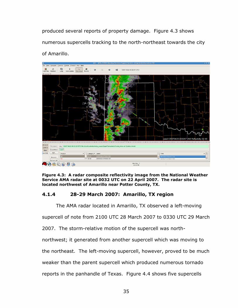
orientation of a stationary front through the region. Figure 4.8 shows

the bowing line segment moving towards the Saint Louis area late in

the morning on 21 July 2006.


Service LSX radar site at 1509 UTC on 21 July 2006.

4.2.3 9 July 2004: Hastings, NE region

The third case of this type was recorded at the Hastings,

Nebraska radar site (UEX) from 0230 UTC to 0700 UTC on 9 July 2004.

A squall-line associated with an outflow boundary from a disintegrating

cold front moved southeast through the area, producing widespread

damage to mostly rural areas. The Hastings case is of note because it

is a classic case of broken areal squall-line development as outlined by

41

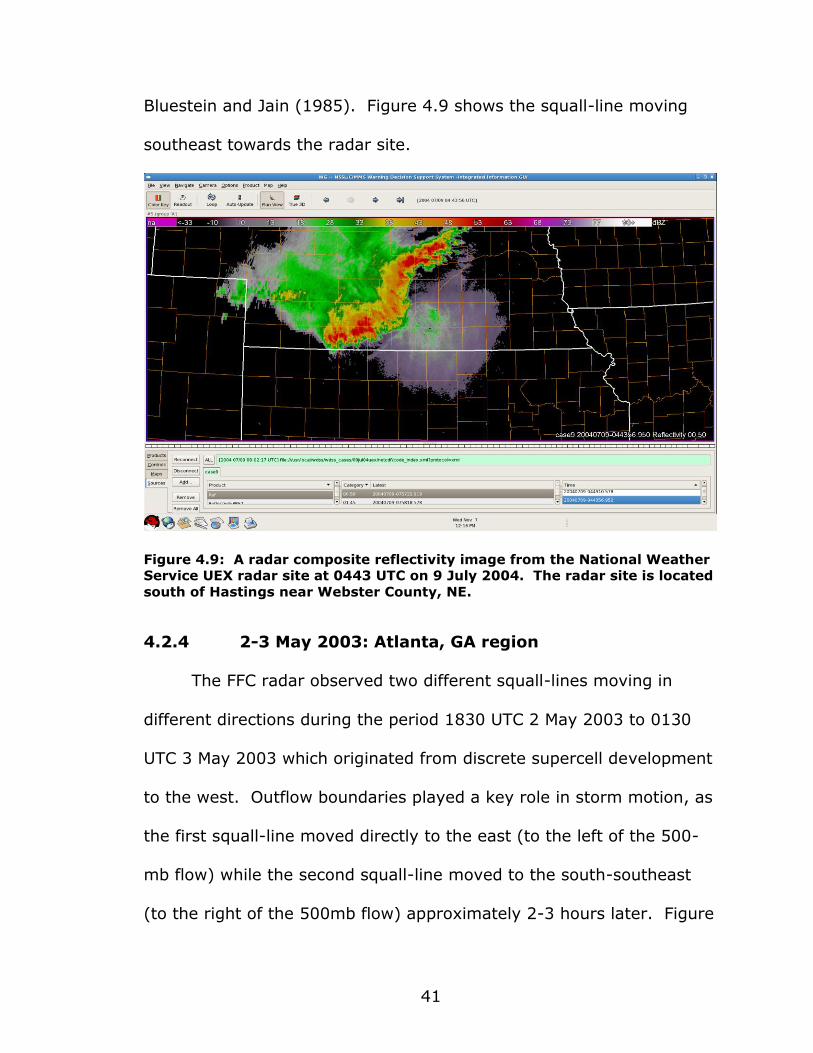
Bluestein and Jain (1985). Figure 4.9 shows the squall-line moving

southeast towards the radar site.


Service UEX radar site at 0443 UTC on 9 July 2004. The radar site is located

south of Hastings near Webster County, NE.

4.2.4 2-3 May 2003: Atlanta, GA region

The FFC radar observed two different squall-lines moving in

different directions during the period 1830 UTC 2 May 2003 to 0130

UTC 3 May 2003 which originated from discrete supercell development

to the west. Outflow boundaries played a key role in storm motion, as

the first squall-line moved directly to the east (to the left of the 500-

mb flow) while the second squall-line moved to the south-southeast

(to the right of the 500mb flow) approximately 2-3 hours later. Figure

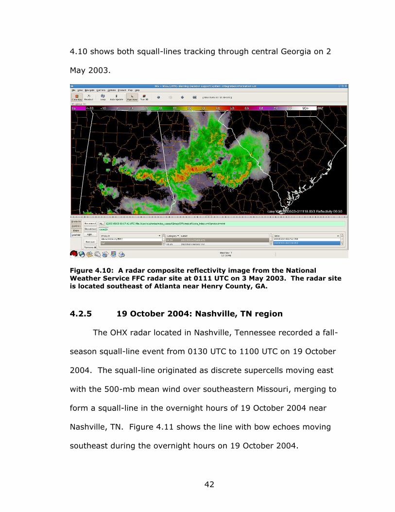
42

4.10 shows both squall-lines tracking through central Georgia on 2

May 2003.

Figure 4.10: A radar composite reflectivity image from the National

Weather Service FFC radar site at 0111 UTC on 3 May 2003. The radar site

is located southeast of Atlanta near Henry County, GA.

4.2.5 19 October 2004: Nashville, TN region

The OHX radar located in Nashville, Tennessee recorded a fall-

season squall-line event from 0130 UTC to 1100 UTC on 19 October

2004. The squall-line originated as discrete supercells moving east

with the 500-mb mean wind over southeastern Missouri, merging to

form a squall-line in the overnight hours of 19 October 2004 near

Nashville, TN. Figure 4.11 shows the line with bow echoes moving

southeast during the overnight hours on 19 October 2004.

43


Weather Service OHX radar site at 0415 UTC on 19 October 2004. The radar

site is located northwest of Nashville near Robertson County, TN.

4.2.6 6 November 2005: Saint Charles, MO region

The LSX radar recorded the last squall-line event in this study

from 0000 UTC to 0530 UTC 6 November 2005 as an unusually strong

low-pressure system tracked across the lower Great Lakes. The

northeast to southwest oriented squall-line formed quickly as discrete

supercells merged over central Missouri. The squall-line tracked to the

east (with individual cells moving northeast along the line) producing

numerous reports of hail and wind damage. Figure 4.12 shows the line

(with cells merged) moving east from Missouri into Illinois during the

overnight hours on 6 November 2005.

44


Weather Service LSX radar site at 0244 UTC on 6 November 2005.

4.3 Multi-cell events

4.3.1 6-7 August 2005: Fort Worth, TX region

The NWS WSR-88D radar site located in Fort Worth, TX (FWS)

observed a multi-cell event from 1830 UTC 6 August 2005 to 0030

UTC 7 August 2005 as daytime instability made the environment

favorable for intense vertical motion and, therefore, thunderstorms.

Since wind speeds at all levels were weak, multi-cell thunderstorms

were the main type of convective mode. Figure 4.13 shows generating

and collapsing cells to the west and east of the Fort Worth radar site.

Since the cells moved very slowly, the risk for flash flooding was

enhanced.

45


Weather Service FWS radar site at 2133 UTC on 6 August 2005. The radar

site is located south of Fort Worth near Johnson County, TX.

4.3.2 19-20 June 2006: Jackson, MS region

The 19-20 June 2006 multi-cell event occurred from 1800 UTC

19 June 2006 to 0000 UTC 20 June 2006 in the Jackson, MS region of

the DGX radar site. The storm propagated across the western side of

the radar area as multi-cell thunderstorms formed across central

Mississippi and moved west into central Louisiana. Outflow boundaries

are a significant contribution to the event as they initiated the storms.

Figure 4.14 shows the cells moving west through Mississippi towards

Louisiana along the outflow boundary.

46


Weather Service DGX radar site at 2030 UTC on 19 June 2006. The radar

site is located east of Jackson near Brandon in Rankin County, MS.

4.3.3 2 July 2006: Tampa Bay, FL region

The mid-summer sea breeze was responsible for these storms as

they moved into the Tampa Bay, Florida region and radar site (TBW).

The storms moved from east to west (with the surface-925-mb flow)

along an outflow boundary easily noticed on radar imagery from 1500

UTC to 2300 UTC. Some of the stronger storms in the case produced

hail just to the north of the Tampa Bay metropolitan area. Figure 4.15

shows the cells moving west along the west-moving outflow boundary,

produced by the sea breeze earlier in the day, towards the Tampa

metropolitan area.

47


Weather Service TBW radar site at 1829 UTC on 2 July 2006. The main

outflow boundary is indicated with arrows. The radar site is located south

of Tampa in Hillsborough County, FL.

4.3.4 28 July 2006: State College, PA region

The fourth case of this type occurred in the State College,

Pennsylvania region and near the CTP radar site as a cold front moved

from west to east across the region. Multi-cellular storms formed in

central Pennsylvania and moved to the east along the front from 1530

UTC to 2030 UTC, staying discrete as they moved though much of

eastern Pennsylvania. Figure 4.16 shows cells moving east through

Pennsylvania along and ahead of the front on 28 July 2006.

48


Weather Service CCX radar site at 1659 UTC on 28 July 2006. The radar is

located west of State College in Centre County, PA.

4.3.5 5 July 2004: Baltimore, MD/Washington, DC region

On 5 July 2004 multiple multi-cell storms affected the Baltimore,

Maryland/Washington, DC area and were detected by the LWX radar

from 1730 UTC to 2330 UTC. An upper-level low moving across

eastern West Virginia late in the morning became the focus for

initiation later at mid-day, with two distinct cells moving in different

directions in northern Virginia late in the afternoon. Figure 4.17 shows

the cells tracking in different directions through West Virginia,

Maryland, and Virginia during 5 July 2004.

49


Weather Service LWX radar site at 1948 UTC on 5 July 2004. The two cells

mentioned in the case study description are indicated with arrows. The

radar is located northwest of Sterling near Loudoun County, VA.

4.3.6 13 June 2004: Memphis, TN region

NWS NQA radar detected multi-cell thunderstorms in this case

on 13 June 2004 which moved west to east across the state. Outflow

boundaries are the focus of the case, evident in radar imagery

throughout the duration of the event from 1700 UTC to 2330 UTC.

4.4 Summary

This study examined eighteen different supercell/squall-

line/multi-cell thunderstorm events, six of each type. There were 25

days worth of radar data, in which 9 were in the supercell category, 8

50

were in the linear category, and 8 were in the multi-cell category. A

total of 53 cells in the following 12 cases were selected for

classification:

Date Site Radar # of Cells Type

12-Mar-2006 Kansas City, MO EAX 5 Supercell

2-Apr-2006 Memphis, TN NQA 4 Supercell

28-Mar-2007 Amarillo, TX AMA 4 Supercell

21-Apr-2007 Amarillo, TX AMA 5 Supercell

7-Apr-2006 Memphis, TN NQA 6 Supercell

19-July-2006 Saint Louis, MO LSX 6 Linear

21-July-2006 Saint Louis, MO LSX 5 Linear

6-Nov-2005 Saint Louis, MO LSX 3 Linear

6-Aug-2005 Fort Worth, TX FWS 3 Multicell

19-Jun-2006 Jackson, MS JAN 4 Multicell

2-Jul-2006 Tampa Bay, FL TBW 5 Multicell

28-Jul-2006 State College, PA CCW 3 Multicell

Table 4.1: Cases and their identified cells (n=53) used for classification in

the study.

Out of the 53 cells tracked, 24 were supercells, 14 were linear cells,

and 15 were multicells.

51

Chapter 5

Results

This study uses several different case studies of supercell, linear,

and multi-cell events. For each type, there are multiple comparisons

which include the mixed-layer convective available potential energy

(MLCAPE), 0-3 km storm relative helicity (SRH), 0-6 km mean wind

speed, 0-6 km wind shear, average thunderstorm motion and speed,

the vorticity generation parameter (VGP), level of the 0°C, -10°C, and

-20°C isotherms, and lastly, the u and v-components of the wind at

those levels. The first section will explain the process of cell

classification by the statistical classifier using pre-existing storm

environmental conditions. Next, the isothermal wind method will be

compared to other predictive cell motion methods. Third, assessments

of parameters by storm type will be made. Finally, the performance of

the isothermal wind method will be explored.

5.1 Classification of Cells with Parameter Information by

Statistical Classifier

In order to create a dataset for classification, the cells in the

study had to be subjectively identified prior to running the classifier.

The initial dataset consisted of 12 different dates from 2006-2007 with

52

53 individually identified cells covering various geographical regions

with the majority in the Midwest and South. As in Lack (2007), the

cases span different seasons so the classifier would identify storm type

independent of time of year and that cases only deal with warm-

season precipitation.

Three different classification types were used in the study and

are summarized in Table 5.1. The rationale for using the types is

explained in Chapter 3.

Classification Type Description

Pulse Thunderstorm (Multicell) Low Shear, CAPE, VGP, SRH

Severe QLCS (Linear) Medium Shear, SRH; Sig. CAPE, VGP

Supercell Sig. Shear, SRH; Medium CAPE, VGP

Table 5.1: The three classification types used within the classification tree

study.

Once the storms were individually identified, a table was

generated with all storm attributes and tagged with one of the three

categories. This information was used to determine the best use of

parameters to determine cell type. The results are classified as a

“tree” with nodes at each branch with represents the best “split” of the

data (Lack 2007). The result is a deterministic solution that labels the

cell in a certain class. For information on the classification tree

scheme, consult Lack (2007), Breiman et al. (1984), or Burrows

(2007).

53

Figure 5.1: Cell classification tree for the 53 cells in the study.

Figure 5.1 shows the classification tree derived from the information

obtained of the 53 cells in the study. The first split using a 0-6

kilometer wind shear value of 58.45 kts results in a separation of

multicell or pulse thunderstorms (low shear) from severe linear cells

and supercells (high speed and/or directional shear), resulting in a

correct analysis of all 15 multicells in the study. Table 5.2 is the cell

array for the multicells used in the study.

The second split using a 0-3 kilometer storm relative helicity

value of 89.5 m2 s-2 separates linear cells with helicities less than 89.5

m2 s-2 from linear cells with helicities grater than 89.5 m2 s-2 or

supercells. This split separated weakly rotating from strongly rotating

54

storms and resulted in a correct analysis of 22 of the 24 supercells

used in the study. Table 5.3 is the supercell array for the study.

CAPE (J kg1) VGP HEL (m2s-2) 0-6 Shear (kts)

Correctly

Identified

840 0.174 20 56.8 Y

1448 0.140 0 39.9 Y

815 0.086 0 35.5 Y

1578 0.123 7 37.4 Y

1129 0.169 19 55.3 Y

1185 0.124 11 37.0 Y

894 0.150 -11 49.7 Y

2888 0.262 34 49.7 Y

3312 0.278 33 47.8 Y

2957 0.179 6 31.4 Y

3174 0.168 -4 30.1 Y

1577 0.142 -5 39.1 Y

270 0.080 39 46.9 Y

1237 0.200 71 56.3 Y

1674 0.254 29 56.9 Y

Table 5.2: Selected output fields for multicells used in the study. VGP is a

dimensionless parameter.

The third and last split of the tree using a MLCAPE value of

1289.5 J kg-1 designated cells with helicities greater than 89.5 m2 s-2

and MLCAPE values of less than 1289.5 J kg-1 as linear cells with the

rest being supercells. This resulted in a correct classification of 9 of

the 14 linear cells. One reason for the drop in accuracy is the severity

of the linear cases and the large MLCAPE and SRH values for some of

the linear cells, which ultimately were not classified correctly. Table

5.4 is the linear cell array for the study.

55

CAPE (J kg1) VGP SRH (m2s-2) 0-6 Shear (kts)

Correctly

Identified

1945 0.370 206 76.7 Y

2997 0.392 190 69.3 Y

3112 0.393 292 67.3 Y

3898 0.319 415 89.9 Y

1629 0.332 187 88.1 Y

1491 0.334 112 87.2 Y

1709 0.313 114 81.0 Y

1664 0.357 265 79.5 Y

2137 0.411 316 81.2 Y

1878 0.361 216 74.5 Y

1500 0.388 318 93.3 Y

2090 0.371 229 87.4 Y

2400 0.415 260 78.1 Y

1945 0.343 230 85.1 Y

1348 0.416 435 103.8 Y

3381 0.380 138 61.1 Y

3303 0.391 159 61.9 Y

2985 0.352 154 63.0 Y

2760 0.488 236 74.0 Y

891 0.191 65 66.2 N

981 0.206 91 65.2 N

1808 0.301 251 65.4 Y

2427 0.367 255 70.2 Y

1890 0.423 402 87.1 Y

Table 5.3: Selected output fields for supercells used in the study. VGP is a


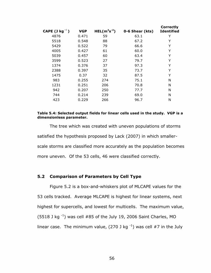
56

Table 5.4: Selected output fields for linear cells used in the study. VGP is a


The tree which was created with uneven populations of storms

satisfied the hypothesis proposed by Lack (2007) in which smaller-

scale storms are classified more accurately as the population becomes

more uneven. Of the 53 cells, 46 were classified correctly.

5.2 Comparison of Parameters by Cell Type

Figure 5.2 is a box-and-whiskers plot of MLCAPE values for the

53 cells tracked. Average MLCAPE is highest for linear systems, next

highest for supercells, and lowest for multicells. The maximum value,

(5518 J kg -1) was cell #85 of the July 19, 2006 Saint Charles, MO

linear case. The minimum value, (270 J kg -1) was cell #7 in the July

CAPE (J kg1) VGP HEL(m2s-2) 0-6 Shear (kts)

Correctly

Identified

4876 0.471 59 63.1 Y

5518 0.548 88 67.2 Y

5429 0.522 79 66.6 Y

4005 0.427 61 60.0 Y

5039 0.457 60 63.4 Y

3599 0.523 27 79.7 Y

1374 0.376 37 97.3 Y

2388 0.397 35 73.7 Y

1475 0.37 32 87.5 Y

983 0.255 274 75.1 N

1231 0.251 206 70.8 N

942 0.207 250 77.7 N

744 0.214 239 69.0 N

423 0.229 266 96.7 N

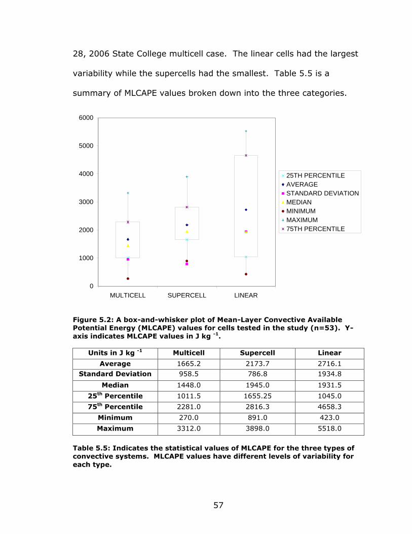
57

28, 2006 State College multicell case. The linear cells had the largest

variability while the supercells had the smallest. Table 5.5 is a

summary of MLCAPE values broken down into the three categories.

0

1000

2000

3000

4000

5000

6000

MULTICELL SUPERCELL LINEAR

25TH PERCENTILE

AVERAGE

STANDARD DEVIATION

MEDIAN

MINIMUM

MAXIMUM

75TH PERCENTILE

Figure 5.2: A box-and-whisker plot of Mean-Layer Convective Available

Potential Energy (MLCAPE) values for cells tested in the study (n=53). Y-

axis indicates MLCAPE values in J kg -1.

Units in J kg -1 Multicell Supercell Linear

Average 1665.2 2173.7 2716.1

Standard Deviation 958.5 786.8 1934.8

Median 1448.0 1945.0 1931.5

25th Percentile 1011.5 1655.25 1045.0

75th Percentile 2281.0 2816.3 4658.3

Minimum 270.0 891.0 423.0

Maximum 3312.0 3898.0 5518.0

Table 5.5: Indicates the statistical values of MLCAPE for the three types of

convective systems. MLCAPE values have different levels of variability for

each type.

58

0

0.1

0.2

0.3

0.4

0.5

0.6


25TH PERCENTILE

AVERAGE

STANDARD DEVIATION

MEDIAN

MINIMUM

MAXIMUM

75TH PERCENTILE

Figure 5.3: A box-and-whisker plot of Vorticity Generation Parameter (VGP)

values for cells tested in the study (n=53). Y-axis indicates VGP values.

A box-and-whiskers plot of the 53 cells tracked is shown in

figure 5.3. Average VGP is highest for linear systems, next highest for

supercells (although the average was almost the same), and lowest for

multicells. The maximum value, 0.548 (dimensionless), was again cell

#85 from the July 19, 2006 Saint Charles case. The minimum value

(0.08) was again from cell #7 in the State College, PA case of July 28,

2006. As with MLCAPE, the linear cells had the highest variability,

while the supercells had the lowest. Table 5.6 is a summary of VGP

values broken down into the three categories.

59

Multicell Supercell Linear

Average 0.169 0.359 0.375


Median 0.168 0.369 0.387

25th Percentile 0.132 0.334 0.252

75th Percentile 0.190 0.392 0.468

Minimum 0.080 0.191 0.207

Maximum 0.278 0.488 0.548

Table 5.6: Indicates the statistical values of VGP for the three types of

convective systems. VGP values have different levels of variability for each

type.

Figure 5.4 is a box-and-whiskers plot of 0-3-kilometer storm

relative helicity (SRH) values. Average SRH is highest for supercells,

next highest for linear systems, and lowest for multicells. The

maximum value (435 m2s-2) was cell #6 of the March 12, 2006

Pleasant Hill case (which is the five-state supercell). The lowest value

(-11 m2s-2) was cell #32 of the June 19, 2006 Jackson case. Linear

cells had the largest variability of SRH, while multicells had the

smallest. Table 5.7 is a summary of SRH values broken down into the

three types of storms.

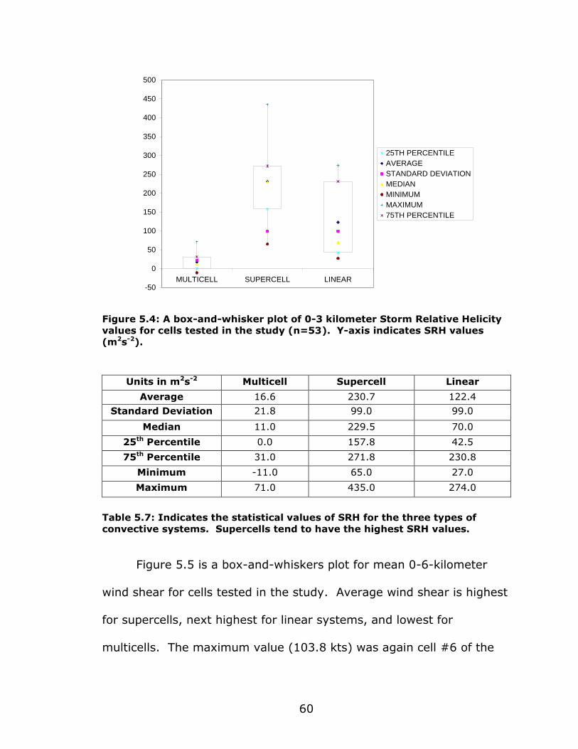
60

-50

0

50

100

150

200

250

300

350

400

450

500


25TH PERCENTILE

AVERAGE

STANDARD DEVIATION

MEDIAN

MINIMUM

MAXIMUM

75TH PERCENTILE

Figure 5.4: A box-and-whisker plot of 0-3 kilometer Storm Relative Helicity

values for cells tested in the study (n=53). Y-axis indicates SRH values

(m2s-2).

Units in m2s-2 Multicell Supercell Linear

Average 16.6 230.7 122.4


Median 11.0 229.5 70.0

25th Percentile 0.0 157.8 42.5

75th Percentile 31.0 271.8 230.8

Minimum -11.0 65.0 27.0

Maximum 71.0 435.0 274.0

Table 5.7: Indicates the statistical values of SRH for the three types of

convective systems. Supercells tend to have the highest SRH values.

Figure 5.5 is a box-and-whiskers plot for mean 0-6-kilometer

wind shear for cells tested in the study. Average wind shear is highest

for supercells, next highest for linear systems, and lowest for

multicells. The maximum value (103.8 kts) was again cell #6 of the

61

March 12, 2006 Pleasant Hill, MO case. The minimum value (30.1 kts)

was cell #43 of the July 2, 2006 Tampa Bay, FL case. Variability of

wind shear was highest in supercells, and lowest in linear systems.

Table 5.8 is a summary of wind shear values broken down into the

three categories of storms.

0

20

40

60

80

100

120


25TH PERCENTILE

AVERAGE

STANDARD DEVIATION

MEDIAN

MINIMUM

MAXIMUM

75TH PERCENTILE

Figure 5.5: A box-and-whisker plot of mean 0-6 kilometer wind shear values

for cells tested in the study (n=53). Y-axis indicates wind shear values

(kts).

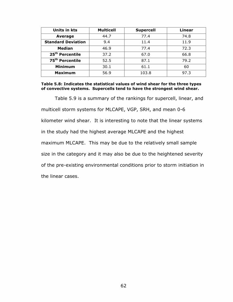
62

Units in kts Multicell Supercell Linear

Average 44.7 77.4 74.8


Median 46.9 77.4 72.3



Minimum 30.1 61.1 60

Maximum 56.9 103.8 97.3

Table 5.8: Indicates the statistical values of wind shear for the three types

of convective systems. Supercells tend to have the strongest wind shear.

Table 5.9 is a summary of the rankings for supercell, linear, and

multicell storm systems for MLCAPE, VGP, SRH, and mean 0-6

kilometer wind shear. It is interesting to note that the linear systems

in the study had the highest average MLCAPE and the highest

maximum MLCAPE. This may be due to the relatively small sample

size in the category and it may also be due to the heightened severity

of the pre-existing environmental conditions prior to storm initiation in

the linear cases.

63

Multicell Supercell Linear

MLCAPE Average 3 2 1

MLCAPE Maximum 3 2 1

VGP Average 3 2 1

VGP Maximum 3 2 1

SRH Average 3 1 2

SRH Maximum 3 1 2

Mean 0-6 Wind Shear Average 3 1 2

Mean 0-6 Wind Shear Maximum 3 1 2

Table 5.9: Rankings of the three different types of storms for selected

parameters in the study.

5.3 Storm Speed

The 53 cells in the study were also tested for similarities in their

velocity versus the velocity of the -20, -10, and 0°C isothermal wind.

Figure 5.6 is a scatterplot of supercells as compared to the -20°C

isothermal wind speed; linear cells compared to the -10°C isothermal

wind speed, and multicells compared to the 0°C isothermal wind

speed. That is, the y=x trendline corresponds to the equality of -20,

-10, or 0°C isothermal wind speed versus the actual cell velocity for

supercells, linear cells, or multicells, respectively. The most

enlightening result of Figure 5.6 is the conclusion that with supercells,

23 of the 24 cells tested moved slower than the -20°C isothermal wind

velocity, with the 24th exactly at the -20°C isothermal wind velocity.

With linear cells, 7 of the 14 moved faster than the -10°C isothermal

64

wind velocity, 1 moved exactly with the -10°C isothermal wind

velocity, and 6 moved slower than the -10°C isothermal wind velocity.

Lastly, with multicells, 12 of the 15 moved faster than the 0°C

isothermal wind velocity, while the other 3 moved slower. As one

moves lower in the atmosphere, the more likely the cell will move

faster than the isothermal wind at that level.

0

10

20

30

40

50

60

70

80

90

0 10 20 30 40 50 60 70 80 90

Cell Velocities (kts)

Iso

the

rma

l W

ind

s (

kts

)

Supercell

Linear

Multicell

Faster

Slower

Figure 5.6: Illustration of velocities of cells tested in the study versus

Isothermal winds. Y=X trendline indicates the equality of the -20, -10, and

0°C isothermal wind velocities to supercell, linear, or multicell velocities

respectively.

65

20

30

40

50

60

70

80

20 30 40 50 60 70 80

-20C Isothermal Wind Speed (kts)

Su

pe

rce

ll S

pe

ed

(k

ts)

0

10

20

30

40

50

60

70

0 10 20 30 40 50 60 70

Linear Speed (kts)

-10

C Iso

the

rma

l W

ind

sp

ee

d (

kts

)

0

5

10

15

20

25

30

35

40

0 5 10 15 20 25 30 35 40

Multicell Speed (kts)

0C

Iso

the

rma

l W

ind

Sp

ee

d (

kts

)

Figure 5.7: Same as Figure 5.14 for A) supercells, B) linear cells, and C)

multicells.

5.4 Performance of Isothermal Wind Method

5.4.1 Direction of Motion of Supercells

As explained in Chapter 3, the height of the 0, -10, and -20°C

Isotherms, the u and v-wind components at said isotherms, the mean

wind speed from 0-6 kilometers, shear from 0-6 kilometers, mean

layer convective available potential energy, 0-3-kilometer storm-

relative helicity, and the vorticity generation parameter as near-storm

environment parameters are derived from RUC-20 data ingested into

WDSS-II. The storm motion and velocity data were derived from the

66

SCIT algorithm within WDSS-II. The conversion of u and v-wind

components into degrees involved the following calculations:

direction = tan-1 )v

u( if u 0, v > 0 (5.1)

= tan-1 +)v

u( 180° if u 0, v < 0 (5.2)

= tan-1 +)v

u( 360° if u 0, v < 0 (5.3)

where u is the u-component of the wind (m s-1) and v is the v-

component. The velocity is then calculated:

velocity = 22 v+u (5.4)

and the value is converted to knots (operational unit used by NWS)

by:

knots = 514.0

velocity. (5.5)

As stated earlier, previous research has shown storms with

stronger (weaker) updrafts will have motion corresponding with higher

(lower) critical winds. Figure 5.11 shows a comparison between actual

storm motion and wind direction (in degrees) at the -20°C isotherm

for 24 cells tracked in the supercell cases. It can be seen that most of

the values lie close to the y=x trendline (storm motion = winds at the

-20°C isotherm).

67

170

190

210

230

250

270

290

310

330

350

170 190 210 230 250 270 290 310 330 350

-20C Isothermal Wind (degrees)

Ac

tua

l S

torm

Mo

tio

n (

de

gre

es

)

Figure 5.8: A comparison between the Actual Storm Direction of Motion

(degrees) and -20°C isothermal wind (degrees) for cells tracked in supercell

cases. The solid line is a trendline of equality.

There are 24 data points in Figure 5.8. The most, six, are from

the April 7, 2006 case in Memphis, while five each are from the March

12, 2006 case in Pleasant Hill and the April 21, 2007 case in Amarillo.

Four are from both the April 2, 2006 case in Memphis and the March

28, 2007 case in Amarillo. On average, results show the actual storm

motion to be only 2.7 degrees to the left of the -20°C isothermal wind

direction with a standard deviation of 11.8 degrees. A correlation

coefficient of 0.91 was found between the -20°C isothermal wind

direction and the actual storm motion, meaning that there is quite a

similarity between the two values. This similarity demonstrates the

usefulness of the -20°C isothermal wind in predicting supercell motion.

Mean squared error for the values was 141.5 degrees squared.

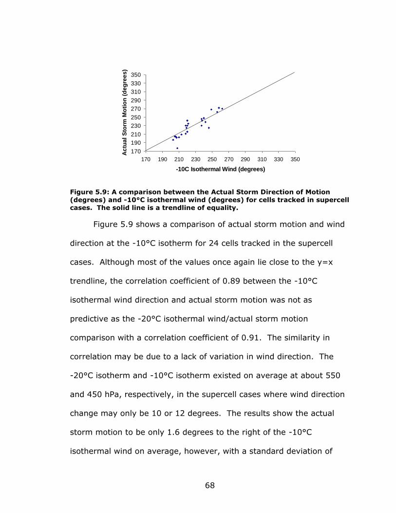
68

170

190

210

230

250

270

290

310

330

350

170 190 210 230 250 270 290 310 330 350


Ac

tua

l S

torm

Mo

tio

n (

de

gre

es

)




Figure 5.9 shows a comparison of actual storm motion and wind

direction at the -10°C isotherm for 24 cells tracked in the supercell

cases. Although most of the values once again lie close to the y=x

trendline, the correlation coefficient of 0.89 between the -10°C

isothermal wind direction and actual storm motion was not as

predictive as the -20°C isothermal wind/actual storm motion

comparison with a correlation coefficient of 0.91. The similarity in

correlation may be due to a lack of variation in wind direction. The

-20°C isotherm and -10°C isotherm existed on average at about 550

and 450 hPa, respectively, in the supercell cases where wind direction

change may only be 10 or 12 degrees. The results show the actual

storm motion to be only 1.6 degrees to the right of the -10°C

isothermal wind on average, however, with a standard deviation of

69

11.9 degrees. Mean squared error for the values was 137.92 degrees

squared.

The motion of cells in the supercell cases was also compared to

the 0°C isothermal wind direction, which Figure 5.10 illustrates. Most

of the values lie close to the y=x trendline again, yet the correlation

coefficient of 0.88 between the 0°C isothermal wind direction and

actual storm motion was not as high as the -20°C isothermal

wind/actual storm motion comparison. On average, the results show

the actual storm motion to be 4.8 degrees to the right of the 0°C

isothermal wind direction with a standard deviation of 11.7 degrees.


170

190

210

230

250

270

290

310

330

350

170 190 210 230 250 270 290 310 330 350

0C Isothermal Wind (degrees)

Actu

al

Sto

rm M

oti

on

(d

eg

rees)


(degrees) and 0°C isothermal wind (degrees) for cells tracked in supercell


70

5.4.2 Direction of Motion of Linear Convective Systems

Figure 5.11 shows a comparison between actual storm motion

and wind direction at the -20°C isotherm for 14 cells tracked in the

linear cases. The most, six, are from the July 19, 2006 case in Saint

Charles, while five are from the July 21, 2006 Saint Charles case.

Three are from the November 6, 2005 Saint Charles case. It can be

seen that all of the values lie above the y=x trendline (actual storm

motion to the right of the isothermal wind), although some of the

points are a close match to the -20°C isothermal wind direction. On

average, results show the actual storm motion to be 28.1 degrees to

the right of the -20°C isothermal wind direction with a standard

deviation of 18.8 degrees. A correlation coefficient of 0.95 was found

between the -20°C isothermal wind direction and linear storm motion,

meaning quite a similarity between the two values. Mean squared

error for the values was 1121.86 degrees squared.

71

210

230

250

270

290

310

330

350

370

390

210 230 250 270 290 310 330 350 370 390

-20C Isothermal Winds (degrees)

Actu

al

Sto

rm M

oti

on

(d

eg

rees)


(degrees) and -20°C isothermal wind (degrees) for cells tracked in linear

cases. The solid line is a trendline of equality. Values over 360 degrees are

cell motions near the 0/360 degree direction discriminator, with 360

degrees added for continuity.

Figure 5.12 shows a comparison of actual storm motion and wind

direction at the -10°C isotherm for the 14 cells tracked in the linear

cases. Once again, most of the values lie nowhere close to the y=x

trendline. On average, actual storm motion is 25.1 degrees to the

right of the -10°C isothermal wind direction with a standard deviation

of 45.5 degrees. A correlation coefficient of 0.97 was found, which

had a higher amount of predictability than the -20°C isothermal

wind/linear storm motion correlation coefficient. Mean squared error

for the values was 858.64 degrees squared.

72

210

230

250

270

290

310

330

350

370

390

210 230 250 270 290 310 330 350 370 390


Actu

al

Sto

rm M

oti

on

(d

eg

rees)






Figure 5.13 illustrates the comparison between actual storm

motion and the 0°C isothermal wind direction for the 14 linear cells.

On average, the actual storm motion was 16.6 degrees to the right of

the 0°C isothermal wind with a standard deviation of 15.7 degrees.

The correlation coefficient of 0.97 once again shows the similarity

between the 0°C isothermal wind direction and linear storm motion.


73

210

230

250

270

290

310

330

350

370

390

210 230 250 270 290 310 330 350 370 390


Actu

al

Sto

rm M

oti

on

(d

eg

rees)

Figure 5.13: A comparison between the Actual Storm Motion (degrees) and

0°C isothermal wind (degrees) for cells tracked in linear cases. The solid

line is a trendline of equality. Values over 360 degrees are cell motions

near the 0/360 degree direction discriminator, with 360 degrees added for

continuity.

For linear cases, the 0°C isothermal wind direction was the most

successful predictor of motion, although the -10°C isothermal wind

direction was successful as well. Once again this may be due to the

small differences in wind direction at the two levels.

5.4.3 Direction of Motion of Multicells


and wind direction at the -20°C isotherm for 15 cells tracked in the

multicell cases. The most, five, are from the July 2, 2006 case in

Tampa Bay, FL. Four are from the June 19, 2006 case in Jackson, MS,

while three are from both the August 6, 2005 Fort Worth, TX case and

the July 28, 2006 State College, PA case. Most of the values do not lie

anywhere near the y=x trendline as expected. Some of the values,

74

however, come very close to 0 or 360 degrees, having somewhat of a

“nyquist” effect on the correlation coefficient. On average, results

show the actual storm motion to be 79.9 degrees to the left of the

-20°C isothermal wind direction, with a standard deviation of 102.0

degrees.

25

75

125

175

225

275

325

375

425

475

525

25 75 125 175 225 275 325 375 425 475 525 575 625 675 725


Actu

al

Sto

rm M

oti

on

(d

eg

rees)


(degrees) and -20°C isothermal wind (degrees) for cells tracked in multicell




A correlation coefficient of 0.89 was found between the -20°C

isothermal wind direction and multi-cell storm motion. Mean squared

error for the values was 1.61 X 10 4 degrees squared.

The 15 multicells and their motions tracked in the study were

then compared to the direction of the -10°C isothermal wind, which

figure 5.15 illustrates. The values lie a bit closer to the y=x trendline,

yet have a lower linear correlation coefficient of 0.82. On average,

75

actual storm motion was 96.8 degrees to the left of the -10°C

isothermal wind direction, with a standard deviation of 100.6 degrees.

Mean squared error for the values was 1.88 X 10 4 degrees squared.

25

75

125

175

225

275

325

375

425

475

525

25 75 125 175 225 275 325 375 425 475 525 575 625 675 725


Actu

al

Sto

rm M

oti

on

(d

eg

rees)


(degrees) and -10°C isothermal wind (degrees) for cells tracked in multicell




Figure 5.16 shows a comparison between the actual storm

motion of the 15 multicells and the 0°C isothermal wind direction.

This comparison had the best correlation coefficient of the three tested

for multicells, at 0.91. The average storm motion was 9.1 degrees to

the left of the 0°C isothermal wind direction with a standard deviation

of 95.6 degrees. Mean squared error for the values was 8620.80

degrees squared. The increased success of the lower-level isotherm in

predicting multicell motion backed the hypothesis stated earlier, as

eight of the fifteen cells’ motions were within 31 degrees of the 0°C

isothermal wind direction.

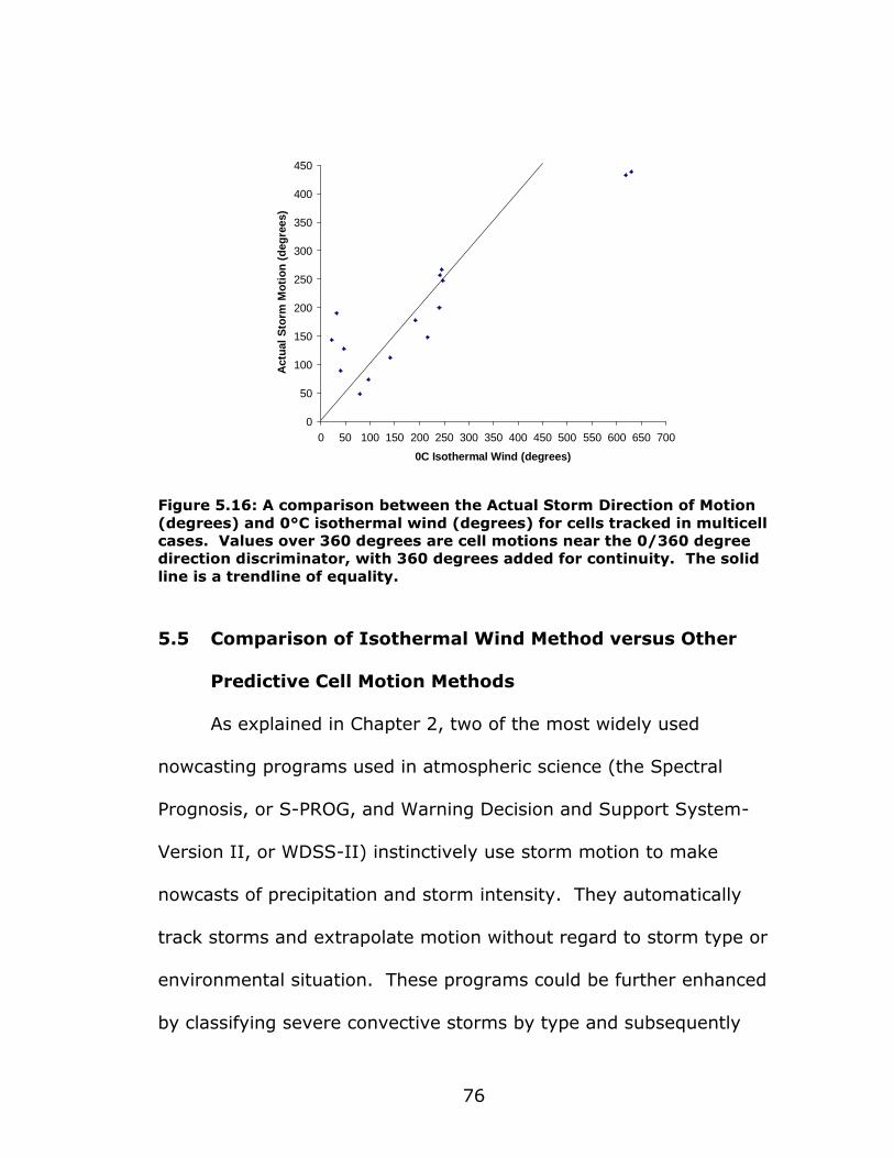
76

0

50

100

150

200

250

300

350

400

450

0 50 100 150 200 250 300 350 400 450 500 550 600 650 700


Actu

al

Sto

rm M

oti

on

(d

eg

rees)


(degrees) and 0°C isothermal wind (degrees) for cells tracked in multicell

cases. Values over 360 degrees are cell motions near the 0/360 degree

direction discriminator, with 360 degrees added for continuity. The solid

line is a trendline of equality.

5.5 Comparison of Isothermal Wind Method versus Other

Predictive Cell Motion Methods

As explained in Chapter 2, two of the most widely used

nowcasting programs used in atmospheric science (the Spectral

Prognosis, or S-PROG, and Warning Decision and Support System-

Version II, or WDSS-II) instinctively use storm motion to make

nowcasts of precipitation and storm intensity. They automatically

track storms and extrapolate motion without regard to storm type or

environmental situation. These programs could be further enhanced

by classifying severe convective storms by type and subsequently

77

forecasting the motion of the storms from this information---along

with existing environmental conditions. Other procedures for

forecasting storm motion based on storm type exist (e.g. Lindsey and

Bunkers 2004; hereafter LB04 for supercells, Corfidi et al. 1996 for

mesoscale convective complexes; hereafter C96, and Marwitz 1972 for

multicells, hereafter M72). They generally use standard-level wind

vectors which may not be appropriate in every case (e.g. the 0-6 km

wind, 850-300-mb wind, and the 0-10-km wind for studies mentioned

earlier, respectively). These wind levels may not always be

representative of the surface layer or cloud layer, but are convenient

for access as long-standing standard atmospheric levels and model

products. On the other hand, the rich variety of model output at

numerous levels allows the use of more flexible product selection from

Rapid Update Cycle (RUC) or Weather Research and Forecasting Model

(WRF) output that could be more closely associated to the motion of a

particular storm.

Supercells σ MSE

-20°C Isothermal Wind (Y=X) 11.8 141.5

-20°C Isothermal Wind (Best Fit) 7.3 104.3

LB04 10.7 150.9

Table 5.10: Comparison of the standard deviation (in degrees) and mean

squared error (in degrees squared) for the Isothermal Wind Method as

opposed to the LB04 0-6 kilometer mean-wind method. While the standard

deviation is lower for LB04, MSE is lower for the Isothermal Wind Method.

78

Table 5.10 is a comparison of the standard deviation and mean

squared error for two Isothermal Wind Methods versus the LB04

method. The first Isothermal Wind Method correlates the storm

direction of motion versus a y=x trendline (actual storm motion =

isothermal wind direction at that level). The second Isothermal Wind

Method correlates the storm direction of motion versus the line of

best-fit for the type of storm indicated.


and wind direction (in degrees) at the -20°C isotherm for 24 cells

tracked in the supercell cases. The equation (storm direction

algorithm) placed in the figure corresponds with the line of best fit.

The other line with slope m =1 indicates a y=x relationship. The 24

supercells tested in the study were tracked using the LB04 method and

compared to the Isothermal Wind Method. The Isothermal Wind

Method had the same linear correlation as LBO4, with a larger

standard deviation and smaller mean squared error. The supercell

storm motion algorithm from the line of best fit can be expressed as

CS=1.3258d-20-78.041 (5.1)

with d-20 = wind direction in degrees at the -20°C isotherm.

79

y = 1.3258x - 78.041

R2 = 0.8271

170

190

210

230

250

270

290

310

330

350

170 190 210 230 250 270 290 310 330 350

-20C Isothermal Wind

Actu

al S

torm

Mo

tio

n



cases. The red line is the y=x trendline, while the blue/black line is the line

of best fit.



opposed to the C96 mean 850-300 mb wind method. Standard deviation

and mean square error are smaller for the Isothermal Wind Method.

Table 5.11 is a comparison of the same statistical parameters for

the Isothermal Wind Method versus the C96 method. The 14 linear

cells tested in the study were tracked using the C96 method. Figure

5.18 shows a comparison of actual storm motion and wind direction at

the -10°C isotherm for the 14 cells tracked in the linear cases. The

Isothermal Wind method again had a smaller standard deviation and

mean squared error.

Linear Systems σ MSE

-10°C Isothermal Wind (Y=X) 16.0 858.6

-10°C Isothermal Wind (Best Fit) 9.4 191.6

C96 16.6 876.4

80

y = 1.2213x - 35.554

R2 = 0.9394

210

230

250

270

290

310

330

350

370

390

210 230 250 270 290 310 330 350 370 390


Actu

al

Sto

rm M

oti

on

(d

eg

rees)



cases. The red line is the y=x trendline, while the blue line is the line of

best fit. Values over 360 degrees are cell motions near the 0/360 degree

direction discriminator, with 360 degrees added for continuity.

Multicells σ MSE

0°C Isothermal Wind (Y=X) 95.6 8620.8

0°C Isothermal Wind (Best Fit) 26.9 2096.9

M72 119.8 13694.5



opposed to the M72 0-10 km mean wind method. The correlation coefficient

is more predictive with less error using the Isothermal Wind Method.

The linear cell storm motion algorithm from the line of best fit can be

expressed as

CL=1.2213d-10-35.554 (5.2)

with d-10 = wind direction in degrees at the -10°C isotherm.

Table 5.12 is the comparison of the Isothermal Wind Method

versus the M72 method. The 15 multicells in the study after testing by

the Isothermal Wind Method were tracked again using the M72

81

method. Figure 5.19 shows a comparison between the actual storm

motion of the 15 multicells and the 0°C isothermal wind direction.

The Isothermal Wind Method had a smaller standard deviation and

mean squared error.

The multi-cell storm motion algorithm from the line of best fit

can be expressed as

CM=0.5625d0+80.910 (5.3)

with d0 = wind direction in degrees at the 0°C isotherm.

y = 0.5625x + 80.91

R2 = 0.8355

0

50

100

150

200

250

300

350

400

450

0 50 100 150 200 250 300 350 400 450 500 550 600 650 700


Actu

al

Sto

rm M

oti

on

(d

eg

rees)


(degrees) and 0°C isothermal wind (degrees) for cells tracked in multicell

cases. 360 degrees is added in some cases for continuity. The red line is

the Y=X trendline, while the blue line is the line of best fit.

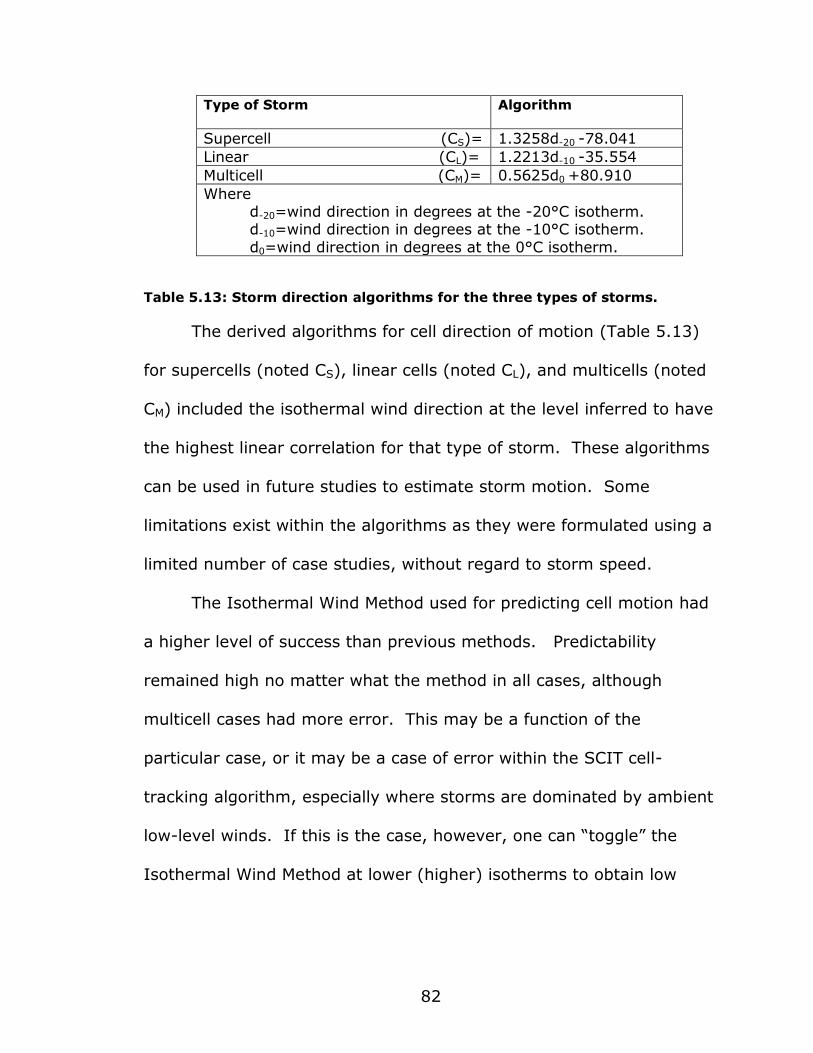
82

Type of Storm Algorithm

Supercell (CS)= 1.3258d-20 -78.041

Linear (CL)= 1.2213d-10 -35.554

Multicell (CM)= 0.5625d0 +80.910

Where d-20=wind direction in degrees at the -20°C isotherm. d-10=wind direction in degrees at the -10°C isotherm.

d0=wind direction in degrees at the 0°C isotherm.

Table 5.13: Storm direction algorithms for the three types of storms.

The derived algorithms for cell direction of motion (Table 5.13)

for supercells (noted CS), linear cells (noted CL), and multicells (noted

CM) included the isothermal wind direction at the level inferred to have

the highest linear correlation for that type of storm. These algorithms

can be used in future studies to estimate storm motion. Some

limitations exist within the algorithms as they were formulated using a

limited number of case studies, without regard to storm speed.

The Isothermal Wind Method used for predicting cell motion had

a higher level of success than previous methods. Predictability

remained high no matter what the method in all cases, although

multicell cases had more error. This may be a function of the

particular case, or it may be a case of error within the SCIT cell-

tracking algorithm, especially where storms are dominated by ambient

low-level winds. If this is the case, however, one can “toggle” the

Isothermal Wind Method at lower (higher) isotherms to obtain low

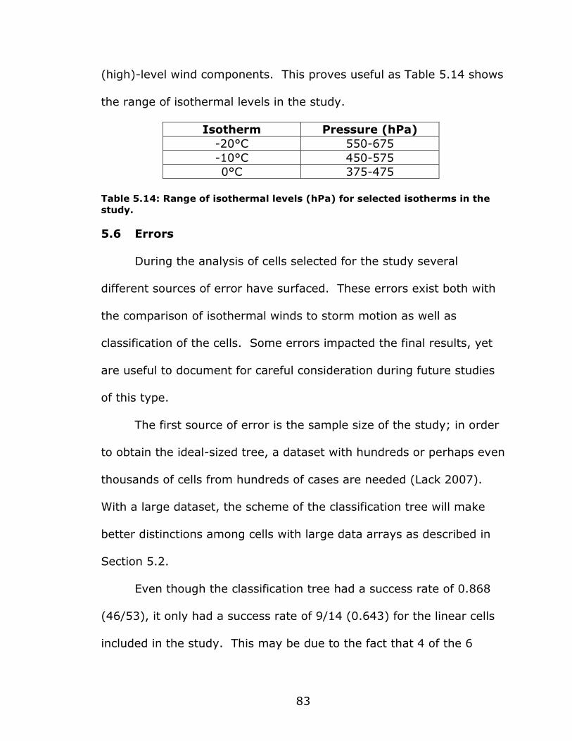
83

(high)-level wind components. This proves useful as Table 5.14 shows

the range of isothermal levels in the study.

Isotherm Pressure (hPa)

-20°C 550-675

-10°C 450-575

0°C 375-475

Table 5.14: Range of isothermal levels (hPa) for selected isotherms in the

study.

5.6 Errors

During the analysis of cells selected for the study several

different sources of error have surfaced. These errors exist both with

the comparison of isothermal winds to storm motion as well as

classification of the cells. Some errors impacted the final results, yet

are useful to document for careful consideration during future studies

of this type.

The first source of error is the sample size of the study; in order

to obtain the ideal-sized tree, a dataset with hundreds or perhaps even

thousands of cells from hundreds of cases are needed (Lack 2007).

With a large dataset, the scheme of the classification tree will make

better distinctions among cells with large data arrays as described in

Section 5.2.

Even though the classification tree had a success rate of 0.868

(46/53), it only had a success rate of 9/14 (0.643) for the linear cells

included in the study. This may be due to the fact that 4 of the 6

84

linear cases included in the study were hybrid cases in which the

convective mode at initiation was different from the convective mode

at the end of the case. Many of the linear cells in those cases were

possibly at one time supercells and this contributes to their supercell

characteristics. When looking at the classification tree, a distinction

was made between linear cells and supercells by MLCAPE. The

distinction is a way of looking at the instability throughout the entire

column of the cell. Intuitively, one would guess that this value would

be higher in supercells. The problem with this assumption was that

many of the values of MLCAPE in the linear cells were higher than

those of the supercell cases, resulting in misclassified cells. VGP was

never used as a discriminator between cells in this study; it was used

in the Lack (2007) study and successfully partitioned rotating storms

from non-rotating storms more effectively than the 0-6 kilometer

mean shear value used as a discriminator in this study.

The selection of the -20, -10, and 0°C isotherms as non-

mandatory levels to look at storm motion was an effective choice. A

more effective choice, however, may have been larger-spaced

isothermal selection with a level closer to the surface. The linear

correlation of storm motion to isothermal wind direction may be higher

with selected thresholds of every 15°C, or 20°C, instead of the 10°C

spacing used in this study. Furthermore, isotherms above 0°C are

85

situated closer to the surface, and may be able to account for the high

variability of multicell motion. The small sample size also may have

had an effect on the overall success of the correlations calculated.

Another source of error may include the calculation of the

average direction and velocity of storm motion in the study. The

method used the direction and velocity of the cell in each radar scan

throughout the life of the cell and averaged those values into a “final”

direction and velocity for use in statistical analysis later. For multicells

and linear cells with little direction change throughout the life of the

storm, this is an effective way to gauge storm motion. However, with

supercells (especially high-precipiatation supercells as noted by

Bunkers et al. 2000), motion (in direction and speed) can vary, and an

average amongst the whole cell life may fail to properly weigh the

importance of key direction changes, splits, or mergers into and out of

the cell. For example, a supercell with a low-level mesocyclone may

deviate up to 20 degrees from previous motion (as shown with 2 cells

in this study). A way to correct the problem would be to automate the

detection of direction change within storms with a size of greater than

a selected threshold for a particular case. This would give a more

accurate and faster description of cell motion and velocity, allowing

nowcasters more time to prepare for severe weather conditions.

86

Another source of error lies within the formulation of the

algorithms to approximate cell motion. The algorithms were

formulated using a line of best fit, yet the number of cells used to

make the line of best fit was less than optimal. Outliers within a storm

type may change the line of best-fit drastically, and therefore, increase

the percentage of error in forecasting the motion of a specific storm

type. Even with the errors that exist, the validity of the algorithms

can subsequently be tested in future studies with more cases and cells.

Data assimilation within WDSS-II may have also contained

errors. An incorrect selection of cells can affect or even corrupt overall

results. The SCIT algorithm within WDSS tends to merge cells

together when in very close proximity (Jankowski 2006, Johnson et al.

1998), small in length along a radial, or shallow cells not covered in

consecutive radar scans. This tends to happen in linear cells with

large areas of the same reflectivity, much like the cells included in this

study. A way to rectify the problem is to perhaps automate the

selection of cells with different mesoscale features with an area-based

tracking algorithm as best described in Johnson et al. (1998). This

algorithm can effectively delineate between cells with similar

attributes.

87

5.7 Discussion

Examining data among the three types of cells in the study

showed a strong linear correlation between the -20°C isothermal wind

direction and supercell motion, a strong linear correlation between the

-10°C isothermal wind direction and linear cell motion, and a

significant linear correlation between the 0°C isotherm and multicell

motion. Cell tracking by isothermal wind direction also performed with

a higher level of predictability than previous studies. Lastly, many of

the cells used in the study were correctly identified by the statistical

classifier using near-storm environmental model data. Knowing the

convective mode of storms at genesis helps the forecaster to make a

deterministic evaluation of storm motion, velocity, severity, and

duration in a given area. Thus, finding a correlation between storm

type and storm motion gives forecasters the chance to make more

accurate forecasts of storm type and where the storms will have an

effect.

The results of the study in applying near-storm environment

model data to the cells identified are summarized in the following

points:

Supercell thunderstorms tend to move with the -20°C

isothermal wind direction; have the highest variability in 0-6

88

kilometer wind shear and move slower than the -20°C

isothermal wind speed.

Cells in linear systems were found to move with the -10°C

and -20°C isothermal wind direction; have the highest

variability in mean layer CAPE, 0-3 kilometer storm relative

helicity, and the vorticity generation parameter and have no

propensity to move slower or faster than the -10°C

isothermal wind speed.

Multicell thunderstorms have a strong linear correlation to the

0°C isothermal wind direction; typically have the lowest

CAPE, shear, VGP, and SRH values and move faster than the

0°C isothermal wind speed.

The results of the study in applying classification tree techniques

are summarized forthwith:

Cell classification with smaller non-rotating storms was more

accurate; the discriminators used to separate types of storms

made intuitive sense.

Cell discriminating between cells in linear systems and

supercells using the MLCAPE parameter resulted in a less than

desirable success rate; the use of VGP is a more successful

89

parameter to use as documented by Lack (2007) and other

previous studies.

Hybrid cases as theorized by Lack (2007) seem to decrease

the success rate of the statistical classifier; more research is

needed in the area to evaluate the significance of this claim.

Additional storm attributes may be needed to more

successfully classify types of storms.

As discussed earlier, the primary goal of evaluating storm type

versus storm motion is to give forecasters a better chance of telling

the public the potential dangers of a given type of storm in a forecast

area. Classification can be used in real-time by forecasters to monitor

particularly severe storms, or to make a historical archive of storms for

different inter-annual time frames. As explained in Lack (2007), the

primary goal of the classification tree scheme is to use the information

given by the model data to input into nowcasting products for cell

morphology purposes.

The objectives and hypotheses for this research were listed for

this study in Chapter 1. The research obtained in this study first notes

that different pre-existing meteorological conditions exist for supercell,

linear, and multicell systems. Second, the classification tree system

successfully classified different storm types in most cases. Looking at

storm motion alone helps in the forecasting process, but does not

90

make a forecast alone. The understanding of storm morphology and

the addition of storm type, if not included or even neglected in a

nowcast, may mean severe conditions can be underestimated, missed,

or even ignored.

91

Chapter 6

Summary and Conclusions

6.1 Summary

Defining conclusively storm motion by storm type has shown to

be one of the least researched topics in the field of atmospheric

science. The aim of this work was to discover if better forecasts of

storm motion could be made by classifying storm type prior to using

and selecting an appropriate nowcast scheme. Nowcasting programs

such as WDSS-II can be further enhanced by classifying severe

convective storms by type and subsequently forecasting the motion of

the storms from this information along with pre-existing environmental

conditions. This study’s second purpose was to identify the pre-

existing meteorological conditions associated with three different types

of convective systems and to use a statistical classifier to separate

cells of different type.

Several different case studies located near NWS radars in

Kansas City, MO (EAX), Memphis, TN (NQA), Amarillo, TX (AMA), Saint

Louis, MO (LSX), Hastings, NE (UEX), Atlanta, GA (FFC), Nashville, TN

(OHX), Fort Worth, TX (FWS), Jackson, MS (JAN), Tampa Bay, FL

(TBW), State College, PA (CCX), Sterling, VA (LWX), and Columbus Air

Force Base, MS (GWX) were examined in this study. Of the cases

92

examined for cell classification, there were 5 supercell cases, 3 linear

cases, and 4 multicell cases. Each of the 18 cases was analyzed using

WDSS-II which uses SCIT to track a cell’s velocity and direction of

motion. The motion of the cells in the 12 cell-classification cases were

then compared to near-storm environmental RUC-20 data of

isothermal wind direction and velocity at the -20, -10, and 0°C

isotherms. Although all of the cases were not used for cell-

classification, the other 6 cases were used as quality-control (i.e.

continuity) for values calculated in the 12 cell-classification studies.

Table 6.1 is a summary of all cases in the study.

93

Date Radar Site Abbr. Storm Type

12-Mar-2006 Kansas City, MO EAX Supercell

02-Apr-2006 Memphis, TN NQA Supercell

28-Mar-2007 Amarillo, TX AMA Supercell

21-Apr 2007 Amarillo, TX AMA Supercell

04-May 2003 Topeka, KS TOP Supercell

07-Apr-2006 Memphis, TN NQA Supercell

19-Jul-2006 Saint Louis, MO LSX Linear

21-Jul-2006 Saint Louis, MO LSX Linear

9-Jul-2004 Hastings, NE UEX Linear

2-May-2003 Atlanta, GA FFC Linear

19-Oct-2004 Nashville, TN OHX Linear

6-Nov-2005 Saint Louis, MO LSX Linear

6-Aug-2005 Fort Worth, TX FWS Multicell

19-Jun-2006 Jackson, MS JAN Multicell

2-Jul-2006 Tampa Bay, FL TBW Multicell

28-Jul-2006 State College, PA CCX Multicell

5-Jul-2004 Washington, DC LWX Multicell

13-Jun-2004 Memphis, TN NQA Multicell

Table 6.1: Cases used in the study.

Overall, the -20°C isotherm did well in predicting storm motion

for all types, but did best with supercells. On average, supercells

moved 2.7 degrees to the left of the -20°C isothermal wind direction

with a correlation coefficient of 0.91. From looking at these values, it

is concluded that wind direction at the -20°C isotherm is a proper

indicator of supercell motion. The -10 and 0°C isothermal wind

directions were not as predictive. However, the 0°C isotherm had

94

some success in predicting multicell motion. Research findings in this

study also indicated that as one moves closer to the surface, the more

likely the cell at that level will move faster than the winds at that same

level. Multicells had the lowest variability and the lowest values of all

parameters tested in the study, while supercells and linear cells had

the highest.

The second objective of this cell was to determine if the

statistical classifier could delineate between cells of different types

based on the pre-existing environmental conditions obtained earlier in

the study. Values of mean-layer convective available potential energy,

0-3 kilometer storm relative helicity, vorticity generation parameter,

and 0-6 kilometer wind shear were gathered for 53 cells. The

information from the cells was placed in the statistical classifier. The

statistical classifier correctly identified all 15 of the multicells, 22 of the

24 supercells, and 7 of the 14 linear cells, for a total success rate of

0.830 (46 of 53 correctly identified cells).

6.2 Future Work

Future work for the evaluation of storm type versus storm

motion includes the accounting and solving of several errors. Such

errors as small sample size, hybrid cases, separating parameters,

95

selection of isotherms, calculation of parameters, and data assimilation

are the foundation for future work to be conducted on this topic.

In order to obtain the ideal-sized tree, a dataset with hundreds

or perhaps even thousands of cells from hundreds of cases are

needed. This leads to future research of perhaps an automated

system of classifying and a historical archive of thousands of cells for

study. Being able to consult the historical archive for research would

lead to more consistent results with storm motion and cell

classification. Hybrid cases in future work could solely be used for a

separate study; this would effectively evaluate the usefulness of the

classifier in delineating cells of different types on an intra-case basis.

Future work to the tree classification system can include parameters of

azimuthal shear, as well as parameters derived from dual-polarization

radar (Lack 2007). A study of merging or splitting cells may also be

needed to update the classifier with those cells that may have different

physical characteristics than others used in this study.

Other research that can be conducted in the future may be to

divide the linear cases into the divisions made by Bluestein and Jain

(1985). This allows researchers to determine the properties of back-

building cells and embedded-areal cells. This may lead to an

explanation of the severity of linear cells in the cases in this study.

The selection of isotherms closer or further from the surface may give

96

nowcasters a better correlation between isothermal wind and

linear/multicell systems. Lastly, the improvement of nowcasting

products with increased automation will give forecasters a chance to

use the data gathered in real-time, and subsequently, forecast for

storm severity or hazardous weather conditions with higher levels of

accuracy and timeliness.

The addition of the future work stated above, along with the

research presented in this study will be more useful for a more

accurate forecast of storm motion by storm type.

97

Appendix A: Cell Identification Matlab Script:

numberID_simp.m (Lack 2007)

%individual identification change time and dates for all

load ('14jul07epz/reflectivity/T20070714_040001.txt');

for i=1:256

for j=1:256

if (T20070714_040001(i,j)<=0)

T20070714_040001(i,j)=0;

end

end

end

[m n]=size(T20070714_040001);

identifycells(30,T20070714_040001);

load ('labeled.txt');

tempmax=max(labeled);

numberofcells=max(tempmax);

imagesc(labeled);

caxis([0 numberofcells]);

colorbar;

%radar data

load ('14jul07epz/echotop/ECHOTOP20070714_040001.txt');

load ('14jul07epz/mesh/MESH20070714_040001.txt');

load ('14jul07epz/posh/POSH20070714_040001.txt');

load ('14jul07epz/vil/VIL20070714_040001.txt');

load ('14jul07epz/vildensity/VILDENSITY20070714_040001.txt');

%ruc 252 data

load ('14jul07epz/mucape/MUCAPE20070714_040000.txt');

load ('14jul07epz/srhelicity/SRHelicity0_3km20070714_040000.txt');

load ('14jul07epz/uwind_0_6km/UWIND_0_6km20070714_040000.txt');

load ('14jul07epz/vwind_0_6km/VWIND_0_6km20070714_040000.txt');

load ('14jul07epz/uwind20C/UWIND20C20070714_040000.txt');

load ('14jul07epz/vwind20C/VWIND20C20070714_040000.txt');

load ('14jul07epz/muvgp/MUVGP20070714_040000.txt');

load ('14jul07epz/muncape/MUCAPE_Normalized20070714_040000.txt');

for i=1:256

for j=1:256

if (MUCAPE_Normalized20070714_040000(i,j)>=1 ||

MUCAPE_Normalized20070714_040000(i,j)<=0)

MUCAPE_Normalized20070714_040000(i,j)=0;

end

end

end

load ('14jul07epz/sfcprestend/RUCSfcPresTendency20070714_040000.txt');

load ('14jul07epz/muehi/MUEHI20070714_040000.txt');

load ('14jul07epz/dcape/DCAPE20070714_040000.txt');

load ('14jul07epz/lapserate/LAPSERATE20070714_040000.txt');

load ('14jul07epz/deepshear/DEEPSHEAR20070714_040000.txt');

load ('14jul07epz/meanrh/MEANRH20070714_040000.txt');

load ('14jul07epz/sfccape/SFCCAPE20070714_040000.txt');

load ('14jul07epz/wetbulbzero/WETBULB20070714_040000.txt');

98

load ('14jul07epz/mucin/MUCIN20070714_040000.txt');

finalarray=0;

for e=1:numberofcells

for i=1:m

for j=1:n

if labeled(i,j)==e

test(i,j)= T20070714_040001(i,j);

echotop(i,j)= ECHOTOP20070714_040001(i,j);

mesh(i,j)= MESH20070714_040001(i,j);

posh(i,j)= POSH20070714_040001(i,j);

vil(i,j)= VIL20070714_040001(i,j);

vildensity(i,j)= VILDENSITY20070714_040001(i,j);

mucape(i,j)=MUCAPE20070714_040000(i,j);

srhel(i,j)=SRHelicity0_3km20070714_040000(i,j);

vgp(i,j)=MUVGP20070714_040000(i,j);

uwind_0_6km(i,j)=UWIND_0_6km20070714_040000(i,j);

vwind_0_6km(i,j)=VWIND_0_6km20070714_040000(i,j);

uwind20C(i,j)=UWIND20C20070714_040000(i,j);

vwind20C(i,j)=VWIND20C20070714_040000(i,j);

ncape(i,j)=MUCAPE_Normalized20070714_040000(i,j);

sfcprestend(i,j)=RUCSfcPresTendency20070714_040000(i,j);

ehi(i,j)=MUEHI20070714_040000(i,j);

dcape(i,j)=DCAPE20070714_040000(i,j);

lapserate(i,j)=LAPSERATE20070714_040000(i,j);

deepshear(i,j)=DEEPSHEAR20070714_040000(i,j);

meanrh(i,j)=MEANRH20070714_040000(i,j);

sfccape(i,j)=SFCCAPE20070714_040000(i,j);

wetbulb(i,j)=WETBULB20070714_040000(i,j);

mucin(i,j)=MUCIN20070714_040000(i,j);

else

test(i,j)=0;

echotop(i,j)= 0;

mesh(i,j)= 0;

posh(i,j)= 0;

vil(i,j)= 0;

vildensity(i,j)= 0;

mucape(i,j)=0;

srhel(i,j)=0;

vgp(i,j)=0;

uwind_0_6km(i,j)=0;

vwind_0_6km(i,j)=0;

uwind20C(i,j)=0;

vwind20C(i,j)=0;

ncape(i,j)=0;

sfcprestend(i,j)=0;

ehi(i,j)=0;

dcape(i,j)=0;

lapserate(i,j)=0;

deepshear(i,j)=0;

99

meanrh(i,j)=0;

sfccape(i,j)=0;

wetbulb(i,j)=0;

mucin(i,j)=0;

end

end

end

%figure;

for i=1:m

for j=1:n

if test(i,j)>0

numpixelstemp(i,j)=1;

else

numpixelstemp(i,j)=0;

end

end

end

numpixelstemp2=sum(numpixelstemp);

numpixelsincell=sum(numpixelstemp2);

if numpixelsincell>20

figure;

imagesc(test);

caxis([0 60]);

colorbar;

%figure;

%imagesc(mucape);

%colorbar;

%figure

%imagesc(srhel);

%colorbar;

%find max and min axes for elipse and area

for i=1:256

for j=1:256

if (test(i,j)>0)

testid(i,j)=1;

else

testid(i,j)=0;

end

end

end

%imagesc(testid);

for degree=1:180

rotimage=rotate_image( degree, testid, [1,256;1,256]);

%figure;

%imagesc(rotimage)

maxaxis(degree)=max(sum(rotimage));

end

axis1=max(maxaxis);

axis2=min(maxaxis);

eliparea=pi()*(axis1/2)*(axis2/2);

testimages=[reshape(test,m*n,1)];

100

echotopimages=[reshape(echotop,m*n,1)];

meshimages=[reshape(mesh,m*n,1)];

poshimages=[reshape(posh,m*n,1)];

vilimages=[reshape(vil,m*n,1)];

vildensityimages=[reshape(vildensity,m*n,1)];

mucapeimages=[reshape(mucape,m*n,1)];

srhelimages=[reshape(srhel,m*n,1)];

vgpimages=[reshape(vgp,m*n,1)];

uwind_0_6kmimages=[reshape(uwind_0_6km,m*n,1)];

vwind_0_6kmimages=[reshape(vwind_0_6km,m*n,1)];

uwind20Cimages=[reshape(uwind20C,m*n,1)];

vwind20Cimages=[reshape(vwind20C,m*n,1)];

ncapeimages=[reshape(ncape,m*n,1)];

sfcprestendimages=[reshape(sfcprestend,m*n,1)];

ehiimages=[reshape(ehi,m*n,1)];

dcapeimages=[reshape(dcape,m*n,1)];;

lapserateimages=[reshape(lapserate,m*n,1)];;

deepshearimages=[reshape(deepshear,m*n,1)];;

meanrhimages=[reshape(meanrh,m*n,1)];;

sfccapeimages=[reshape(sfccape,m*n,1)];;

wetbulbimages=[reshape(wetbulb,m*n,1)];;

mucinimages=[reshape(mucin,m*n,1)];;

for i=1:numpixelsincell

statarray(i)=0;

statarrayechotop(i)=0;

statarraymesh(i)=0;

statarrayposh(i)=0;

statarrayvil(i)=0;

statarrayvildensity(i)=0;

statarraymucape(i)=0;

statarraysrhel(i)=0;

statarrayuwind_0_6km(i)=0;

statarrayvwind_0_6km(i)=0;

statarrayuwind20C(i)=0;

statarrayvwind20C(i)=0;

statarrayvgp(i)=0;

statarrayncape(i)=0;

statarraysfcprestend(i)=0;

statarrayehi(i)=0;

statarraydcape(i)=0;

statarraylapserate(i)=0;

statarraydeepshear(i)=0;

statarraymeanrh(i)=0;

statarraysfccape(i)=0;

statarraywetbulb(i)=0;

statarraymucin(i)=0;

end

j=1;

for i=1:65536

if testimages(i)>0

statarray(j)=statarray(j)+testimages(i);

101

j=j+1;

end

end

k=1;

for i=1:65536

if mucapeimages(i)>0

statarraymucape(k)=statarraymucape(k)+mucapeimages(i);

k=k+1;

end

end

l=1;

for i=1:65536

if srhelimages(i)>0

statarraysrhel(l)=statarraysrhel(l)+srhelimages(i);

l=l+1;

end

end

o=1;

for i=1:65536

if uwind_0_6kmimages(i)~=0

statarrayuwind_0_6km(o)=statarrayuwind_0_6km(o)+uwind_0_6kmimages(i);

o=o+1;

end

end

p=1;

for i=1:65536

if vwind_0_6kmimages(i)~=0

statarrayvwind_0_6km(p)=statarrayvwind_0_6km(p)+vwind_0_6kmimages(i);

p=p+1;

end

end

y=1;

for i=1:65536

if uwind20Cimages(i)~=0

statarrayuwind20C(y)=statarrayuwind20C(y)+uwind20Cimages(i);

y=y+1;

end

end

z=1;

for i=1:65536

if vwind20Cimages(i)~=0

statarrayvwind20C(z)=statarrayvwind20C(z)+vwind20Cimages(i);

z=z+1;

end

end

q=1;

for i=1:65536

if vgpimages(i)>0

statarrayvgp(q)=statarrayvgp(q)+vgpimages(i);

q=q+1;

end

end

102

r=1;

for i=1:65536

if ncapeimages(i)>0

statarrayncape(r)=statarrayncape(r)+ncapeimages(i);

r=r+1;

end

end

s=1;

for i=1:65536

if sfcprestendimages(i)~=0

statarraysfcprestend(s)=statarraysfcprestend(s)+sfcprestendimages(i);

s=s+1;

end

end

t=1;

for i=1:65536

if ehiimages(i)>0

statarrayehi(t)=statarrayehi(t)+ehiimages(i);

t=t+1;

end

end

aa=1;

for i=1:65536

if dcapeimages(i)>0

statarraydcape(aa)=statarraydcape(aa)+dcapeimages(i);

aa=aa+1;

end

end

bb=1;

for i=1:65536

if lapserateimages(i)>0

statarraylapserate(bb)=statarraylapserate(bb)+lapserateimages(i);

bb=bb+1;

end

end

cc=1;

for i=1:65536

if deepshearimages(i)>0

statarraydeepshear(cc)=statarraydeepshear(cc)+deepshearimages(i);

cc=cc+1;

end

end

dd=1;

for i=1:65536

if meanrhimages(i)>0

statarraymeanrh(dd)=statarraymeanrh(dd)+meanrhimages(i);

dd=dd+1;

end

end

ee=1;

for i=1:65536

if sfccapeimages(i)>0

statarraysfccape(ee)=statarraysfccape(ee)+sfccapeimages(i);

103

ee=ee+1;

end

end

ff=1;

for i=1:65536

if wetbulbimages(i)>0

statarraywetbulb(ff)=statarraywetbulb(ff)+wetbulbimages(i);

ff=ff+1;

end

end

gg=1;

for i=1:65536

if mucinimages(i)>0

statarraymucin(gg)=statarraymucin(gg)+mucinimages(i);

gg=gg+1;

end

end

hh=1;

for i=1:65536

if echotopimages(i)>0

statarrayechotop(hh)=statarrayechotop(hh)+echotopimages(i);

hh=hh+1;

end

end

ii=1;

for i=1:65536

if meshimages(i)>0

statarraymesh(ii)=statarraymesh(ii)+meshimages(i);

ii=ii+1;

end

end

jj=1;

for i=1:65536

if poshimages(i)>0

statarrayposh(jj)=statarrayposh(jj)+poshimages(i);

jj=jj+1;

end

end

kk=1;

for i=1:65536

if vilimages(i)>0

statarrayvil(kk)=statarrayvil(kk)+vilimages(i);

kk=kk+1;

end

end

ll=1;

for i=1:65536

if vildensityimages(i)>0

statarrayvildensity(ll)=statarrayvildensity(ll)+vildensityimages(i);

ll=ll+1;

end

end

meanintensityincell=mean(statarray);

104

maxintensityincell=max(statarray);

minintensityincell=min(statarray);

standdevincell=std(statarray);

maxechotopincell=max(statarrayechotop);

maxmeshincell=max(statarraymesh);

maxposhincell=max(statarrayposh);

maxvilincell=max(statarrayvil);

maxvildensityincell=max(statarrayvildensity);

meanmucapeincell=mean(statarraymucape);

meansfccapeincell=mean(statarraysfccape);

meansrhelincell=mean(statarraysrhel);

meanuwind_0_6kmincell=mean(statarrayuwind_0_6km);

meanvwind_0_6kmincell=mean(statarrayvwind_0_6km);

meanuwind20Cincell=mean(statarrayuwind20C);

meanvwind20Cincell=mean(statarrayvwind20C);

meanvgpincell=mean(statarrayvgp);

maxvgpincell=max(statarrayvgp);

meanncapeincell=mean(statarrayncape);

meansfcprestendincell=mean(statarraysfcprestend);

meanehiincell=mean(statarrayehi);

meandcapeincell=mean(statarraydcape);

meanmucinincell=mean(statarraymucin);

meanlapserateincell=mean(statarraylapserate);

meandeepshearincell=mean(statarraydeepshear);

meanwetbulbincell=mean(statarraywetbulb);

meanrhincell=mean(statarraymeanrh);

ratio=axis1/axis2;

finalarrayheader=char('CellID','CellSize','MaxdBZ','MeandBZ','MindBZ','StddBZ','Echo

Top','POSH','MESH','VIL','VILDENSITY','MeanUwind(km/h)','MeanVwind(km/h)','Mean

Uwind20C(km/h)','MeanVwind20C(km/h)','MeanSRHel','MeanMUCAPE','MeanSfcCape'

,'MeanMUCIN','MeanDCAPE','MUVGP','MaxVGP','NCAPE','SFCPRESTEND','EHI','lapsera

te','deep shear','wet bulb 0 z','mean RH','majaxis','minaxis','ratio','ellipseArea','storm

type 1-linear 2-svr linear 3-pulse 4-svr pulse 5-other 6-supercell 7-line w/supercell');

finalarray(e,1)=e;

finalarray(e,2)=numpixelsincell;

finalarray(e,3)=maxintensityincell;

finalarray(e,4)=meanintensityincell;

finalarray(e,5)=minintensityincell;

finalarray(e,6)=standdevincell;

finalarray(e,7)=maxechotopincell*3280.83989501;

finalarray(e,8)=maxposhincell;

finalarray(e,9)=maxmeshincell*0.03937007874;

finalarray(e,10)=maxvilincell;

finalarray(e,11)=maxvildensityincell;

finalarray(e,12)=(meanuwind_0_6kmincell*1.852/6);

finalarray(e,13)=(meanvwind_0_6kmincell*1.852/6);

finalarray(e,14)=(meanuwind20Cincell*1.852/6);

finalarray(e,15)=(meanvwind20Cincell*1.852/6);

finalarray(e,16)=meansrhelincell;

finalarray(e,17)=meanmucapeincell;

finalarray(e,18)=meansfccapeincell;

105

finalarray(e,19)=meanmucinincell;

finalarray(e,20)=meandcapeincell;

finalarray(e,21)=meanvgpincell;

finalarray(e,22)=maxvgpincell;

finalarray(e,23)=meanncapeincell;

finalarray(e,24)=meansfcprestendincell*-1;

finalarray(e,25)=meanehiincell;

finalarray(e,26)=meanlapserateincell;

finalarray(e,27)=meandeepshearincell;

finalarray(e,28)=meanwetbulbincell;

finalarray(e,29)=meanrhincell;

finalarray(e,30)=axis1;

finalarray(e,31)=axis2;

finalarray(e,32)=ratio;

finalarray(e,33)=eliparea;

if(ratio>3.5 && maxintensityincell<53 && numpixelsincell>=500)

finalarray(e,34)=1;

elseif (ratio>3.5 && maxintensityincell>53 && meanvgpincell<0.2 &&

numpixelsincell>=500)

finalarray(e,34)=2;

elseif (ratio<3.5 && numpixelsincell<500 && maxintensityincell<53)

finalarray(e,34)=3;

elseif (ratio<3.5 && numpixelsincell<500 && maxintensityincell>53)

finalarray(e,34)=4;

elseif (ratio<3.5 && numpixelsincell>=500 && maxintensityincell>53 &&

meanvgpincell>0.2)

finalarray(e,34)=6;

elseif (ratio>3.5 && numpixelsincell>=500 && maxintensityincell>53 &&

meanvgpincell>0.2)

finalarray(e,34)=7;

else

finalarray(e,34)=5;

end

statarray=0;

statarraymucape=0;

statarraysrhel=0;

statarrayuwind_0_6km=0;

statarrayvwind_0_6km=0;

statarrayuwind20C=0;

statarrayvwind20C=0;

statarrayvgp=0;

statarrayncape=0;

statarraysfcprestend=0;

statarrayehi=0;

statarraymucin=0;

statarraydcape=0;

statarraysfccape=0;

statarraydeepshear=0;

statarraylapserate=0;

statarraymeanrh=0;

statarraywetbulb=0;

106

statarrayechotop=0;

statarraymesh=0;

statarrayposh=0;

statarrayvil=0;

statarrayvildensity=0;

end

end

107

Appendix B: Cell Matching Matlab Script: identifycells.m

(Lack 2007)

function [genimage, coords,intensities]=identifycells(tol,X)

%nx = 40 ;ny = 28

%load Sakis-Z.dat %truth

%trueimage=reshape(Sakis_Z(:,8),ny,nx)';

% [testimage truecoords trueintensities]=identifycells(20,truecastimage);

%load Sakis-yS.dat %forecast

%forecastimage=reshape(Sakis_yS(:,8),ny,nx)';

% [testimage forecastcoords forecastintensities]=identifycells(20,forecastimage);

% testimage=imread('testimage.bmp')

% testimage=identifycells(.3,testimage);

% [testimage coords]=identifycells(.3,0);

% [testimage coords]=identifycells(.3,testimage);

%close all

scrsz = get(0,'ScreenSize');

figure('Position',[1 scrsz(4) scrsz(3) scrsz(4)/2])

tmp=colormap('jet');

%tmpI=flipud(tmp);

%colormap(tmpI)

colormap(tmp)

set(gca,'Color','w')

set(gcf,'Color','w')

if X==0

[X1,X2] = ndgrid(-5:.2:5, -5:.2:5);

X = .5*exp(-rand(1)*(X1+1+4*rand(1)).^2 - (X2+4*rand(1)).^2)+.5*exp(-

rand(1)*(X1+rand(1)).^2 - rand(1)*5*(X2+rand(1)).^2)+.5*exp(-rand(1)*2*(X1-

3+2*rand(1)).^2 - (X2-2-rand(1)*5).^2);

end

XXX=X;

oldtol=tol;

subplot(1,2,1,'align')

imagesc(X)

caxis([0 60])

%caxis([-1 4])

%caxis([-100 400])

colorbar

%axis('image')

genimage=X;

%t1 = num2str(tol);

%S1 = strvcat('tol=',t1);

%title(S1);

minval=min(min(X));

if minval<0

X=X+abs(minval)+.000000000001;

tol=tol+abs(minval)+.000000000001;

minval=.000000000001;

end

maxval=max(max(X));

108

if tol<minval

tol=minval;

end

if tol>maxval

tol=maxval-.000001;

end

[m n]=size(X);

% get rid of low intensities

for i = 1:m

for j = 1:n

if X(i,j)<tol

X(i,j)=minval;

end

end

end

[X taggedimage]=findboundaries(tol,X);

subplot(1,2,2,'align')

imagesc(X)

caxis([0 60])

%caxis([-100 400])

colorbar

%axis('image')

%t1 = num2str(tol);

%S1 = strvcat('new tol=',t1);

%title(S1);

im=X+zeros(m,n)*min(min(X));

backApprox = blkproc(im,[15 15],'min(x(:))');

backApprox = double(backApprox)/255; % Convert image to double.

backApprox256 = imresize(backApprox, [m n], 'bilinear');

%figure, imshow(backApprox256) % Show resized background image.

im = im2double(im); % Convert I to storage class of double.

I2 = im - backApprox256;

I2 = double(max(min(I2,1),0)); % Clip the pixel values to the valid range.

%figure, imshow(I2)

I3 = imadjust(I2, [0 max(I2(:))], [0 1]); % Adjust the contrast.

bw=I3>0.2; % Make I3 binary using a threshold value of 0.2.

[labeled,numObjects] = bwlabel(bw,8);% Label components.

numObjects;

%figure

%subplot(3,1,1)

%imagesc(I3);

%colorbar

%axis('image')

%subplot(3,1,2)

%imagesc(bw)

%colorbar

109

%axis('image')

%subplot(3,1,3)

%map = hot(numObjects+1); % Create a colormap.

%imshow(labeled+1,map); % Offset indices to colormap by 1.

%colorbar

%axis('image')

%rect = [1 1 m n];

%grain=imcrop(labeled, rect); % Crop a portion of labeled.

grain=imfeature(labeled,'all');

allgrainsarea=[grain.Area];

allgrainscenter=[grain.Centroid];

allgrainsboundingbox=[grain.BoundingBox];

%allgrainsarea;

%[boundaryi boundaryj]=find(boundary);

%do this for all grains

[t no]=size(find(allgrainsarea>40));

%figure

count=1;

sizemat=1;

coords=zeros(numObjects*m*n,3);

intensities=zeros(numObjects,3);

labeled;

%cellintensities=zeros(m*n,1);

for i=1:numObjects

% idx = find([grain.Area]==allgrainsarea(i));

if allgrainsarea(i)>40

Y = ismember(labeled,i);

% subplot(no,1,count)

count=count+1;

XX=zeros(m,n)+minval;

for i1=1:m

for j1=1:n

if Y(i1,j1)==1

XX(i1,j1)=XXX(i1,j1);

end

end

end

cellintensities=findintensities(oldtol,XX);

intensities(count-1,1)=min(cellintensities);

intensities(count-1,2)=mean(cellintensities);

intensities(count-1,3)=max(cellintensities);

[Y1 taggedimage]=findboundaries(0.1,Y);

[i2 i1]=find([taggedimage]==2);

r=size(i1);

coords(sizemat:(sizemat+r-1),1)=i1;

coords(sizemat:(sizemat+r-1),2)=-i2;

coords(sizemat:(sizemat+r-1),3)=count-1;

sizemat=sizemat+r;

% figure

110

% imagesc(taggedimage)

% figure

% imagesc(XX)

% colorbar

% axis('image')

% grain(i)

end

end

dlmwrite('labeled.txt',labeled,' ');

imagesc(labeled)

colorbar;

coords=coords(1:(sizemat-1),:);

intensities=intensities(1:(count-1),:);

%allgrainsarea(find(allgrainsarea>3));

111

References

Baldwin, M.E., J.S. Kain, and S. Lakshmivarahan, 2005: Development of an Automated Classification Procedure for Rainfall Systems. Monthly

Weather Review, 133, 844-862.

Bluestein, H.B., and M.H. Jain, 1985: Formation of Mesoscale Lines of Precipitation: Severe Squall Lines in Oklahoma During the Spring. J.

Atmos. Sci., 42, 1711-1732.

Breiman, L., J.H. Friedman, R.A. Olshen, and C.J. Stone, 1984: Classification and Regression Trees. Wadsworth & Brooks/Cole

Advanced Books and Software, Monterey, California.

Browning, K.A., and F.H. Ludham, 1960: Radar Analysis of a

Hailstorm. Tech. Note No. 5, Contract AF61 (052)-254, Dept. of Meteorology, Imperial College, London, 109 pp.

Bunkers, M.J., B.A. Klimowski, J.W. Zeitler, R.L. Thompson, and M.L.

Weisman, 2000: Predicting Supercell Motion Using a New Hodograph Technique. Wea. Forecasting, 15, 61-79.

Burrows, W.R., 2007: Dynamical-Statistical Models for Lightning

Prediction to 48-hr Over Canada and the United States. Preprints: 5th Conference on Artificial Intelligence Applications to Environmental

Science, San Antonio, TX.

Charba, J., and Y. Sasaki, 1971: Structure and Movement of the

Severe Thunderstorms of 3 April 1964 as Revealed From Radar and Surface Mesonetwork Data Analysis. J. Meteor. Soc. Japan, 49, 191-

214.

Chisholm, A.L., 1966: Small-Scale Structure of Alberta Hailstorms. M.Sc. thesis, Dept. of Meteorology, McGill University, Montreal, 73 pp.

Corfidi, S.F., J.H. Merritt, and J.M. Fritsch, 1996: Predicting the

Movement of Mesoscale Convective Complexes. Wea. Forecasting, 11, 41-46.

Dixon, M. and G. Weiner, 1993: TITAN: Thunderstorm Identification,

Tracking, Analysis, and Nowcasting – A Radar-based Methodology. Journal of Atmospheric and Oceanic Technology, 10, 785-797.

112

Finley, C.A., W.R. Cotton, and R.A. Pielke Sr., 2001: Numerical Simulation of Tornadogenesis in a High-Precipitation Supercell. Part I:

Storm Evolution and Transition into a Bow Echo. J. Atmos. Sci., 58, 1597-1629.

Fovell, R.G., and P.-H. Tan, 1996: Why Multicell Storms Oscillate.

Preprints, 18th Conf. Severe Local Storms, San Francisco, CA, Amer. Met. Soc., 186-189.

Fox, N.I., G.L. Limpert, W.T. Gilmore, J.L. Miranda, A. Schnetzler, N.

Miller, A. Koleiny and S.A. Lack, 2007: The Sensitivity of Object-Based Nowcasts to Object Threshold Selection. 22nd Conference on Weather

Analysis and Forecasting, Amer. Met. Soc., Park City, UT.

_______, and J.W. Wilson, 2005: Very Short Period Quantitative

Precipitation Forecasting. Atmospheric Science Letters, 6, 7-11.

Jankowski, D.M., 2006: Forecasting Storm Duration Using Radar Storm Tracking. M.Sc. thesis, Dept. of Soil, Environmental, and Atmospheric

Sciences, University of Missouri, 97 pp.

Johnson, J.T., P.L. Mackeen, A. Witt, E.D. Mitchell, G.J. Stumpf, M.D. Elits, and K.W. Thomas, 1998: The Storm Cell Identification and

Tracking Algorithm: An Enhanced WSR-88D Algorithm. Wea. Forecasting, 13, 263-276.

Lack, S.A., 2007: Cell Identification, Verification, and Classification

Using Shape Analysis Techniques. D.Phil. dissertation, Dept. of Soil, Environmental, and Atmospheric Sciences, University of Missouri, 147

pp.

________, N.I. Fox and A.C. Micheas, 2007: An Evaluation of a

Procrustes Shape Analysis Verification Tool Using Idealized Cases. 22nd Conference on Weather Analysis and Forecasting, Amer. Met. Soc.,

Park City, UT.

Lakshmanan, V., V. DeBrunner, and R. Rabin, 2002: Nested Partitions Using Texture Segmentation. Southwest Symposium on Image

Analysis and Interpretation, IEEE, Santa Fe, NM.

Lindsey, D.T., and M.J. Bunkers, 2004: Observations of a Severe, Left-Moving Supercell on 4 May 2003. Wea. Forecasting, 20, 15-22.

113

Lynn, R. and V. Lakshmanan, 2002: Virtual Radar Volumes: Creation,

Algorithm Access and Visualization. 21st Conference on Severe Local Storms, Amer. Met. Soc., San Antonio, TX.

Maddox, R.A., 1980: Mesoscale Convective Complexes. Bull. Amer.

Meteor. Soc., 61, 1374-1387.

Marwitz, J.D., 1972a: The Structure and Motion of Severe Hailstorms. Part II: Multicell Storms. J. Appl. Meteor., 11, 180-188.

Micheas, A.C., N.I. Fox, S.A. Lack, and C.K. Wikle, 2007: Cell

Identification and Verification of QPF Ensembles Using Shape Analysis Techniques. Journal of Hydrology, 343, 105-116.

Moller, A.R., C.A. Doswell III, M.P. Foster, and G. R. Woodall, 1994:

The Operational Recognition of Supercell Thunderstorm Environments

and Storm Structures. Wea. Forecasting, 9, 327-347.

Moncrieff, M.W., 1978: The Dynamic Structure of Two-Dimensional Steady Convection in Constant Shear. Quart. J.Roy. Meteor. Soc.,

104, 543-567.

Pinto, J., C. Kessinger, B. Hendrickson, D. Megenhardt, P. Harasti, Q. Xu, P. Zhang, Q. Zhao, M. Frost, J. Cook, and S. Potts, 2007: Storm

Characterization and Short Term Forecasting Using a Phased Array Radar. 33rd Conference on Radar Meteorology, Cairns, Queensland,

Australia.

Rasmussen, E.N., and J.M. Straka, 1998: Variations in Supercell Morphology. Part I. Observations of the Role of Upper-Level Storm-

Relative Flow. Mon. Wea. Rev., 126, 2406-2421.

A FORMAL EVALUATION OF STORM TYPE VERSUS STORM...

Documents

Transcript of A FORMAL EVALUATION OF STORM TYPE VERSUS STORM...