A forecasting model for the requests for MRI scansessay.utwente.nl/67963/1/vanSchaik_MA_MB.pdf · A...

A forecasting model for the requests for MRI scans

Author: Jurre van Schaik, BSc

Supervisors UT:

Prof. Dr. Ir. Erwin W. Hans

Gréanne Leeftink, MSc

Supervisors MST:

Drs. Irma de Vries-Blanken

Marcel Koenderink, MSc

2

Management summary

Problem description

This study investigates the arrival of patients in need of an MRI at the diagnostics department of a

hospital. At this moment it is unclear for the diagnostics department how many patients will arrive

with an MRI request and which department they come from. Every patient arrives unannounced,

which means that there is also no insight in how busy it will be the next weeks or month. Patients are

sent to the diagnostics department by the various specialties, but communication and collaboration

between departments is lacking.

Objective of the research

The objective of the research is forecasting the number of MRI requests that will be received by the

diagnostics department in the coming six weeks. Such a forecast allows scheduling of patients and a

more efficient allocation of personnel.

Approach

To solve this problem we develop a causal forecasting model in Excel, which uses scheduled number

of consultations as input variables and predicts the number of MRIs needed in the coming six weeks.

This model is partly based on the model developed by Ooms (Ooms, 2014), which is a model for

forecasting the amount of OR days by the Orthopedic Department in the Medisch Spectrum Twente

(MST). We extensively analyze the historical data of last year by using data on both the outpatient

clinics and of the diagnostics department. We hypothesize that the amount of consultations at the

outpatient clinic will influences the number of MRI requests for the diagnostics department. We

perform a correlation analysis to check this hypothesis.

Measurements/findings

We have used historical data (Jan-Dec 2014) of both the outpatient clinics and the diagnostics

department and managed to link 7865 MRI requests (74.6%) to the consultations that led to these MRI

requests. We extensively analyzed these data and found that there is indeed a strong correlation

between first visit and follow up consultations and a moderate correlation between emergency and

peer consultation. The specialties that contribute the most MRIs are: Neurology (27%), Orthopedics

(19%), Surgery (12%), General Practitioners (7%), Neurosurgery (7%), Cardiology (4%) and

Otorhinolaryngology (4%).

Model

Our forecasting model predicts the number of MRI requests per week in a six week planning horizon.

As input values for the model we use two different methods. The first part is a causal forecast method

3

which uses the number of planned First Visit Consultation and Follow up Consultations per week for

the departments Neurology, Orthopedics, Surgery, Neurosurgery, Cardiology and

Otorhinolaryngology. For the General Practitioners and other specialties we assumed a constant

amount of MRI requests per week. For the second part we use the time based methods: Exponential

Smoothing and Moving Average which uses the difference between the previous demand and the

forecasts of the last five weeks as input values. The outcome of the model shows the forecasted MRI

requests for the next six weeks in total and per specialty.

To validate the model we used the number of first visit and follow up consultations in the period of

January 2014 to December 2014 (week 2 to week 47). We compared the forecasted outcomes of the

model with the dates the diagnostics department scheduled the MRIs. Our forecast model has a Mean

Average Percentage Error (MAPE) of 8.0% and a correlation of 0.72.

Conclusions

Our forecast model can be used as a tool to forecast MRI requests and can help the diagnostics

department with the allocation of personnel and scheduling of patients in order to reduce the variation

in access time. Furthermore it can be used by the diagnostics department as a negotiation and

communication method to other specialties to give insight in their variation and to allocate different

MRI slots to specialties.

Recommendations

We recommend the MST to keep track of MRI requests, from which specialty the MRI requests come

from and when the MRI is requested as it is required to run our model. Using the model without these

data is possible, but will decrease its forecasting power. Furthermore we recommend the diagnostics

department to get access to the data of the number of consultations specialties have scheduled for

the coming six weeks. These data help improve the outcome of the model. We recommend MST not

to implement this model immediately, but assess its forecasting strength during a six month shadow

run. After a successful implementation this research and model can be adapted for use in other

applications as well, such as forecasting of CT requests.

4

Preface

I got my Bachelor's degree in Technical Medicine in 2012 when I decided to do something else and

started with a pre-master Industrial Engineering and Management. After following two years of various

courses I started with my Master's Assignment at the MST and 14 months later I am about to finish my

Master's thesis. A lot has happened this last period, good and bad things. I was really enthusiastic

about this assignment and really wanted to collaborate, but it did not always go as I wanted. Words

did not come to me and I had trouble focusing. I doubted my decision to change to another Master,

although I knew that I really liked the topics and work field. But I kept writhing and doing research and

eventually with a massive sprint at the end, I managed to finish this thesis before starting my next

adventure, the Eerst De Klas Traineeship.

I thank my family, friends and Erwin Hans for believing in me and supporting me even when I did not

believe in it anymore. I can imaging it was not easy for seeing me struggling, but you are the reason I

kept going on. In December 2014 I joined the graduation group of the University of Twente, they

helped me by stimulating me to continue with my research and showed me the progress I made; thank

you for that. I want to thank Irma de Vries and Marcel Koenderink for answering my questions about

the MST and providing me with the correct data.

I really enjoyed solving the problem and building the forecasting model and I am grateful for this

opportunity. The model I made can be helpful to the MST and the patients in need of an MRI. I am

proud of the end result and I wish to help the MST further with the implementation of this model. In

Appendix B – Manual Forecasting ModelAppendix B – Manual Forecasting Model I included a manual

for the MST to use and I will be available to answer questions or solve problems.

Enschede, August 2015

Jurre van Schaik

5

Contents Management summary ........................................................................................................................... 2

Preface ..................................................................................................................................................... 4

1 Introduction ..................................................................................................................................... 7

1.1 Medisch Spectrum Twente and diagnostics department ....................................................... 7

1.2 Problem Description ................................................................................................................ 8

1.3 Research Objective .................................................................................................................. 8

2 Context Description ....................................................................................................................... 10

2.1 Care Pathway ......................................................................................................................... 10

2.1.1 Outpatient Clinic ............................................................................................................ 11

2.1.2 Diagnostics department ................................................................................................ 13

2.2 Planning and control ............................................................................................................. 15

2.2.1 Planning in the Outpatient Clinic ................................................................................... 17

2.2.2 Planning and scheduling in the diagnostics department .............................................. 17

2.3 Performance .......................................................................................................................... 18

2.3.1 Access time .................................................................................................................... 18

2.3.2 Throughput .................................................................................................................... 19

2.4 Conclusion ............................................................................................................................. 21

3 Extensive Data Analysis ................................................................................................................. 22

3.1 Outpatient Clinic .................................................................................................................... 22

3.2 Diagnostics department ........................................................................................................ 23

3.3 Correlation Analysis ............................................................................................................... 25

3.4 Explanatory Factors ............................................................................................................... 30

3.5 Conclusions ............................................................................................................................ 33

4 Forecast Model MRI Demand ........................................................................................................ 34

4.1 Input values ........................................................................................................................... 34

4.2 Black box ................................................................................................................................ 35

4.3 Output ................................................................................................................................... 37

6

4.4 Validation of the model ......................................................................................................... 38

4.5 Other Forecasting Methods .................................................................................................. 40

4.5.1 Moving Average ............................................................................................................. 41

4.5.2 Exponential Smoothing ................................................................................................. 43

4.5.3 Comparison ................................................................................................................... 43

4.5.4 Improving current model .............................................................................................. 44

4.6 Conclusion ............................................................................................................................. 47

5 Conclusion ..................................................................................................................................... 49

6 Discussion and Recommendations ................................................................................................ 51

References ............................................................................................................................................. 53

Appendix A – Implementation of the forecasting Model ...................................................................... 54

Appendix B – Manual Forecasting Model ............................................................................................. 56

7

1 Introduction

This report is about forecasting the number of patients coming from outpatient clinics whom have a

referral for an MRI at the diagnostics department in the Medisch Spectrum Twente (MST). With the

use of correlation analysis on historical data of the outpatient clinics and the diagnostics department

a model has been built to forecast the arrival of patients for up to six weeks in advance.

Chapter 1 is an introduction to the report. After a description about the Medisch Spectrum Twente

and the diagnostics department (1.1) we describe the problem (1.2) and come up with the research

objective (1.3). Chapter 2 follows with a description of the context and the current performance of the

outpatient clinics and the diagnostics department. We do an extensive data analysis of historical data

and a correlation analysis in Chapter 3. In Chapter 4 we build the model which will be used at the

diagnostics department to predict the arrival of patients who need an MRI. We end with the conclusion

in Chapter 5 and the discussion and some recommendations in Chapter 6.

1.1 Medisch Spectrum Twente and diagnostics department

Medisch Spectrum Twente (MST) is with approximately 3700 general employees and 235 medical

specialists one of the biggest non-academical hospitals in the Netherlands. On a yearly basis

approximately 520.000 outpatients visit the hospital, this results to 35.000 day care admissions. There

are around 34.000 ordinary admissions with a total of 175.000 nursing days.

MST is together with five other top teaching hospitals (Canisius-Wilhelmina Hospital, Catharina-

hospital, Martini Hospital, Onze Lieve Vrouwe Gasthuis, and St. Antonius Hospital) part of Santeon

Hospitals. Together they have one of the biggest laboratories of the Netherlands and they treat around

10 percent of all patients in the Netherlands (academic hospitals included). The collaboration between

these hospitals leads, besides knowledge sharing, to new innovations and improved treatment

methods.

In the region of Twente, MST has three hospitals and two outpatient clinics. Two of the hospitals are

located in Enschede and one in Oldenzaal, the outpatient clinics are located in Haaksbergen and Losser.

The catchment in the region of MST is around 264.000 people. In 2016 a new, modern hospital in the

center of Enschede with 620 beds will be opened (Medisch Spectrum Twente, 2012). In order to fit

into the new hospital, the board wants to reduce 170 fulltime hours. To achieve an economic end

result the board wants to get an higher labor productivity and reduce the number of diagnostics and

get more procurement savings (Medisch Spectrum Twente, 2013).

The number of patients who rely on the diagnostics department is growing rapidly, especially those in

need of an MRI. This results in higher access times for the MRI and higher total throughput time for

8

individual patients in the care pathway. There are several causes for this trend. First of all, extended

research has opened up a lot more possibilities for the MRI. What was not possible to scan a few years

back because of the quality of the scan or the techniques required, is now a standard procedure.

Another reason for these increasing access times could be the growth of the overall number of

patients. Patients grow older, and the disorders are more complex due to comorbidity. This also means

that the need for medical imaging grows. In contrast, the MRI itself is being further developed

(Koenderink, 2010). In 2010, the radiology department of the MST purchased a 3 Teslan MRI, which

can produce more detailed scans and uses less scanning time. Through this purchase more capacity is

available. Still, access times for an MRI are still growing.

1.2 Problem Description

The number of patients in need of an MRI differ from day to day. The diagnostics department has no

insight in the number of patients who will be in need of a diagnostics procedure. It is not known

beforehand how many MRI requests will arrive each day, where they come from and therefore how

busy it will be in the next week or month. Furthermore, there is little communication between the

departments and there is a lack of collaboration. Consultation visit data are available, but it is not being

used for this purpose. Insight in the amount of upcoming MRI requests will make scheduling of patients

and allocation of employees more efficient.

1.3 Research Objective

The objective of the research is:

To develop a forecasting model that uses consultation visit data to predict upcoming MRI requests for

a six week period.

To attain the research objective we will answer the following research questions:

1. What does the current care pathway for patients who arrive at the outpatient clinic and need

an MRI at the diagnostics department look like?

Chapter 2 describes the research context of the outpatient clinic and the diagnostics department

including its performance such as access time and throughput. We have to know what the different

clinical pathways to the diagnostics department are. Also the number of patients and the division of

the different inputs have to be known per department per workday.

1. Is there a correlation between the different consultations and the requested MRIs?

Chapter 3 is an extended data analysis which uses data from the outpatients clinics and the diagnostics

department to analyze a possible correlation between the number of consultations and the requested

9

MRIs from these consultations. It also explains what this means and how we may use it to build a model

to forecast the arrival of patients at the diagnostics department in need of an MRI.

2. What input, calculations and output do we need to make a model to forecast the arrival of

patients at the diagnostics department in need of an MRI.

In Chapter 4 we build our model. We determine what we need to transform this information to build

a reliable model which the diagnostics department can use as a tool to indicate the arrival of patients

in need of an MRI.

3. What configuration and recommendations would be most beneficial for the diagnostics

department??

Chapter 5 describes the conclusions of this research proposal. Chapter 6 describes the discussion and

further recommendations to adapt the model.

10

2 Context Description

This chapter describes the research context. In Section 2.1 we analyze the process by following the

care pathway of the patient from outpatient clinic to the diagnostics department. . Section 2.2

describes the planning and control of the outpatient clinic and diagnostics department. In Section 2.3

we research the performance of the system by calculating the access time and throughput of the

system. Finally in Section 0 we will end with a conclusion.

2.1 Care Pathway

The care pathway of a patient is the route a patient follows when arriving at the hospital to the point

the patient leaves the hospital (Figure 1). In other words a whole care pathway starts with opening a

new DOT and ends with closing this DOT. A DOT is a diagnosis-related group used in the Netherlands

as the basis of payment for care provided by medical specialists and hospitals (Busse et al., 2013),

(Gartner & Kolisch, 2014).

For new patients, the process starts with a referral from the general practitioner to a specialist. The

patient makes an appointment by the outpatient clinic or gets an invitation from the outpatient clinic

with an appointment date. After visiting the outpatient clinic it may be needed to perform some tests

in a lab or use diagnostics. If this is the case an appointment is needed at the lab or diagnostics and at

the outpatient clinic afterwards to discuss the results. When treatment with medicine is sufficient, a

new recurrent appointment will be made. If surgery is required, the patient will go to the preoperative

screening and will have an appointment at the Admissions office. On the day of the surgery, the patient

will arrive at the ward. From the ward the patient will go to the holding, the OR and, after the surgery,

to the Recovery Room. After waking up, he/she will return to the ward until dismissal. Sometimes the

patient will need to go to the diagnostics department again to check whether a drain is placed correctly

or to assess the effect of the operation on the tissue. After discharge the patient will make a new

appointment with the specialist for a checkup at a later moment.

Figure 1 Care Pathway of patients in the MST, divided by follow up and first visit consultation

11

2.1.1 Outpatient Clinic

In the outpatient clinic new and recurrent patients arrive. New patients are patients new to the care

pathway, so those for whom a new DOT starts. Most of these patients arrive after a consult with a

general practitioner. Recurrent patients are patients who come for a checkup, patients whose DOT is

still opened. The last type of patients are patients who had to go for lab or diagnostics and return to

discuss the outcomes with the specialist. These appointments and the walk-in principle appointments

at the lab or diagnostics department are considered the same.

Appointments in a hospital are called consults and the period of January 1 to December 16 2014, there

were around 475.000 consults out of 43 different specialties (69 including sub-specialties) in the MST.

Most specialties have an outpatient clinic. There are in total 13 different consultation codes (Internal

Operation Codes). Most of these consultations are being held at the outpatient clinic, some

consultations are from the inpatient clinic or the emergency room. These consultations can be divided

in 8 different types: First visit consultation, follow up consultation, emergency consultation, peer

consultation, multidisciplinary consultation, outside office consultations, co-treatment and others, see

Table 1 (Nederlandse Zorgautoriteit, 2011a).

Internal Operation Code Internal Operation Description Consultancy type

090613 First visit consultation (old or new patient) by radiotherapist First Visit

090614 Follow up consultation by radiotherapist Follow Up

190009 Peer consultation Peer

190010 Multidisciplinary consultation Multidisciplinary

190013 Follow up consultation Follow Up

190015 Emergency consultation at the ER Emergency

190016 Emergency consultation outside the ER Emergency

190017 Co-treatment (for IC co-treatment see 039672). Co-treatment

190049 National neonatal follow-up protocol Other

190060 First visit consultation First Visit

190063 Intensive consult for the purpose of extra care Other

ZCB Outside office consultations Outside office

ZHERN Follow up consultation Follow Up

Table 1 The consultation types used in the MST in 2014 and the consultation types we use

12

First visit consultation (FVC)

Type of outpatient consultation whereby the patient consults a specialist for the first time with

a new demand for care. This consult is aimed at the determination of a diagnosis and the

discussion of the policy conform the (believed) decease and treatment. This type of

consultation is always the start of a new clinical pathway.

Follow up or repeat consultation (FUC)

Type of outpatient consultation whereby the patient consults a specialist to discuss the

progress of the treatment, the results of (blood) tests or diagnostic imaging, or as a checkup

after a treatment.

Emergency consultation (EC)

Face-to-face consultation between a patient and a specialist when there are acute care needs.

This can be on the emergency department, but also on a different department.

Peer consultation (PC)

A diagnostic or screening contact of a medical specialist with a patient during a clinical in-take

for another specialty, at the request of the responsible medical specialist.

Multidisciplinary consultation (MC)

Type of outpatient consultation with a face-to-face contact between patient and at least two

medical specialist of different departments.

Outside office consultations (OOC)

Consultations which takes place after or before office times.

Co-treatment (CTC)

Type of consultation whereby a medical specialist at the request of another department joins

the treatment in the same care pathway.

Other consultations (OC)

Other type of consultations, mostly very specialized consultations such as “follow-up of

neonatal IC (190049)” and “intensive consultation for the purpose of carefully considering

different treatments (190063)”.

13

2.1.2 Diagnostics department

There are different kind of diagnostic methods in the diagnostics department such as: echo, X-Ray, CT,

MRI or Rontgen. This research will focus solely on MRI, though findings may be transferable to other

diagnostic methods.

Most specialties use MRI as a diagnostic. MRI or Medical Resonance Imaging is an imaging technique

which uses the phenomena of nuclear magnetic resonance. The MRI sends an excitation pulse into the

tissue, the atomic nucleus starts to spin around its axis. This movement depends on the strength of

the pulse and the sort of atom. The energy the atom nucleus has gained will be released in the form

of electromagnetic waves. The MRI has antennas measuring these electromagnetic waves. The amount

of radiation is proportional of the amount of the hydrogen density. Together with the relaxation times

and the density a 3-D picture can be formed (van Oosterom & Oostendorp, 2008).

In

Table 2 the number of consultations and MRI request in the MST is shown per year and specialty. In

the period of January 1 to December 16 2014 almost 11.000 MRIs have been performed.

Specialty # Consults # MRIs Specialty # Consults # MRIs

Radiotherapy 7451 279 Urology 17411 215

Cardiology 33090 466 Otolaryngology 35346 405

Internal Medicine 43478 342 Paediatrics 18314 123

Pulmonology 21277 99 Orthopedics 33181 2049

Gastroenterology 16518 394 Other Specialists 7120 36

Rheumatology 14712 173 Rehabilitation 2763 20

Neurology 24321 2911 Cardiothoracic Surgery 1059 6

Surgery 79565 1284 Psychiatry 7443 1

Dermatology 17807 1 Intensivists 5 10

Ophthalmology 22368 46 Radiology 613 0

Neurosurgery 5938 700 Oral Surgery 17429 48

Gynecology 29454 89 Clinical Neurophysiology 2 2

Plastic Surgery 9458 129 Psychology 5410 0

Anesthesiology 3750 146 General Practitioners 0 759

Total 475283 10733

14

Table 2 Number of consultations per specialty in the MST (Jan-Dec 2014), Business Objects MST

The biggest MRI users are the specialties: Neurology, Orthopedics and Surgery. Together they have

more than 58% of the total number of MRI request (see Figure 2), which is around 6244 MRI requests

of the total of 10733 requests. It is remarkable that there are more MRIs than consultations for the

intensivists. This may be caused by these MRIs being emergency MRIs.

Figure 2 Percentages of MRI requests per specialty in the MST (N=10733 MRIs in the period of Jan-Dec 2014), Business Objects MST

Specialty # Consults # MRIs Specialty # Consults # MRIs

Radiotherapy 7451 279 Urology 17411 215

Cardiology 33090 466 Otolaryngology 35346 405

Internal Medicine 43478 342 Paediatrics 18314 123

Pulmonology 21277 99 Orthopedics 33181 2049

Gastroenterology 16518 394 Other Specialists 7120 36

Rheumatology 14712 173 Rehabilitation 2763 20

Neurology 24321 2911 Cardiothoracic Surgery 1059 6

Surgery 79565 1284 Psychiatry 7443 1

Dermatology 17807 1 Intensivists 5 10

Ophthalmology 22368 46 Radiology 613 0

Neurosurgery 5938 700 Oral Surgery 17429 48

Gynecology 29454 89 Clinical Neurophysiology 2 2

Plastic Surgery 9458 129 Psychology 5410 0

Anesthesiology 3750 146 General Practitioners 0 759

Total 475283 10733

Neurology27%

Orthopedics18%

Surgery11%General Practitioner

8%

Neurosurgery7%

Cardiology4%

Gastroenterology4%

Internal Medicine4%

Otolaryngology3%

Radiotherapy3%

Rheumatology2%

NeurologyOrthopedicsSurgeryGeneral PractitionerNeurosurgeryCardiologyGastroenterologyInternal MedicineOtolaryngologyRadiotherapyRheumatologyPaediatricUrologyAnasthesiaGynecologyPlastische chirPulmonologyRadiologyOral SurgeryOther SpecialistsPhysiatryOphthalmologyPsychiatryCardiothoracic SurgeryIntensivistsClinical Neurophysiology

15

The arrival pattern of patients in need of MRI is complex, because of the various routes to get an MRI.

This makes it hard to schedule patients (Green, Savin, & Wang, 2006), (Carpenter, Leemis, Papir,

Phillips, & Phillips, 2011), (Godin & Wang, 2010).

2.2 Planning and control

In this section we describe the planning and scheduling of the appointments for patients in the

outpatient clinic (Section 2.2.1) as well as in the diagnostics department (Section 2.2.2). In the

diagnostics department we also describe the allocation of personnel and the accessibility of the MRIs.

There is decision making on different managerial and planning levels involved when running a hospital. To focus

our research, this section discusses these different levels and decides on which level the forecasting model could

support planning, based on the hierarchical framework of (van Houdenhoven, 2007), Figure 3.

The Managerial domains are:

Medical planning

Medical planning includes the planning of medical activities. These medical decisions are made by

specialists and includes diagnoses and treatment. Typical performance indicators are quality of care or

research output.

Resource capacity planning

The resource capacity planning deals with efficiently using the hospital’s scarce resources, such as

personnel, Operation Rooms, or MRIs. Typical performance indicators are utilization, overtime, and

underutilization.

Material coordination

Material coordination deals with the distribution of all kinds of materials to support the primary

process. It includes functions like inventory control and purchasing. Typical performance indicators are

service rate and response time.

Financial planning

Financial planning includes all functions regarding hospital finances, such as financial planning and

control and investment planning. Typical performance indicators are profitability, liquidity and

solvability.

16

Figure 3 Framework for hospital planning and control (van Houdenhoven, 2007)

The four hierarchical levels used in this framework are:

Strategic planning

Strategic planning is planning based on long-term objectives or mission statements of an organization.

For example the design of building a new hospital, where to allocate the diagnostics department and

whether or not to acquire an extra MRI scanner. These decisions are mostly over the course of years.

Tactical planning

Tactical planning is based on medium-term objectives and deals with actual patients. For example how

many and where do I allocate the personnel operating the MRI scanner? How many slots do I reserve

for emergency patients? These decisions are mostly over the course of weeks or months.

Operational offline planning

Operational offline planning deals with the day-to-day control of expected activities. For example the

scheduling patients who need an MRI. These decisions are mostly over the course of days or weeks.

Operational online planning

Operational online planning is the last hierarchical level. It involves all control mechanisms that deals

with monitoring and reacting to unforeseen events. For example an emergency patient arrives and

needs an MRI, or dealing with a no show. These decisions are mostly over the course of minutes or

hours.

In our research we will focus on the Resource Capacity planning on an offline operational level.

17

2.2.1 Planning in the Outpatient Clinic

For the planning in the outpatient clinic we will focus on operational offline and online planning. There

is a difference in planning at the outpatient clinic for first visit consultations and follow up

consultations. There are also differences between the outpatient clinics, every specialty has its own

way of scheduling. This research focuses on the overall method.

Patients who want a first visit consultation have to get a referral from the General Practitioner. The

General Practitioner sends the referral to the outpatient clinic via fax or digital means. The outpatient

clinic checks the referral and selects the best specialist and consultation matching the demand of the

patient. The patients gets a proposal for an appointment date via the mail. The date of this proposal is

based on a first come first serve principle. A new appointment has to be made when a patient is not

available this date.

If a patient needs a follow up consultation after the first visit consultation, the patient goes to the desk

and schedules a new appointment. The time for this follow up consultations is often shorter than the

first visit consultation, since the anamnesis is already done. This is also done on first come first serve

principle, but with the same specialist.

When the outpatient clinic gets an emergency patient, it depends on the type of emergency when the

patient is helped. There are no special emergency block reserved, but the patient just gets added to

the queue.

2.2.2 Planning and scheduling in the diagnostics department

In this section we will focus on operational offline and online planning. Section 2.3 and Chapter 3 will

focus on strategic planning and tactical planning.

The scheduling of appointments at MST's diagnostics department is currently being done in Excel by

the MRI administration. The administration gets paper forms from the other specialties or a phone call

to schedule a patient. A patient gets an appointment in a predefined block corresponding to his

medical treatment. The Head specialist Radiology determines when and which types of blocks to book.

If a block is booked, only that type of scan is allowed (e.g. the upper extremities). As a result the access

time for MRI can differ between blocks and specialties. Within a block the scheduling is done on a First

Come First Serve (FCFS) principle, with the obvious exception of emergency patients. Some empty

spots remain in the roster, and eventually these are being filled by the specialist or the laboratory

technician for emergency patients.

18

The duration of an appointment is based on the actual scan time plus the time a patient has to change

(7 minutes). These times are fixed for every type of scan, which means that it can be possible that an

appointment does not fit in a block. This will leave a gap into the schedule.

Emergency patients will be planned 24 hours in advance in the reserved emergency slots. Real

emergencies are done between regular blocks.

2.3 Performance

In this section we describe the performance of outpatient clinic and diagnostics department, using

access time (Section 2.3.1) and the throughput of the care pathway (Section 2.3.2).

2.3.1 Access time

The access time is the time between the MRI request and the actual appointment and scan. Since 2005

there is a norm called: 'treeknorm'. This treeknorm has been conceived and implemented by health

insurance companies and health care providers as a solution to increasing waiting lists. The name

suggests that the treeknorm is a norm, though not true. There are no consequences when the

treeknorm is being exceeded and therefore the treeknorm is more of a directive (vergelijken-

zorgverzekering.net, 2015). Since 2010 all health care providers are obligated to publish their access

times (Nederlandse Zorgautoriteit, 2011). According to the treeknorm for diagnostics the access time

should be no more than 4 weeks. The access time of MRI in the MST from July 2013 to May 2014 can

be seen in Figure 4. The access time is growing in the last few months and exceeding the treeknorm

regularly (Medisch Spectrum Twente, 2014).

Figure 4 Access time of the MRI with and without contrast in the MST including the Treeknorm (Jul-May 2013), RADOS MST

The access time of the MRI is partly based upon supply and demand. In the Netherlands it is allowed

to go to the hospital you like, even if you only want an MRI. When the demand is high, the access time

of the MRI will grow, which leads to patients leaving the hospital to take an MRI elsewhere, for example

to the ZGT (Ziekenhuis Groep Twente) or to an independent MRI Center. The same is happening the

other way around.

01234567

15-jul 15-aug 15-sep 15-okt 15-nov 15-dec 15-jan 15-feb 15-mrt 15-apr 15-mei

We

eks

MRI without contrast MRI with contrast Treeknorm

19

2.3.2 Throughput

In the MST in the period of January 1 to December 16 2014, there were around 475.000 consultations.

These resulted in almost 11.000 MRI requests (Table 3). Neurology and Neurosurgery generate the

most MRI request per consult (12 percent) followed with Orthopedics (6 percent). Intensivist and

clinical neurophysiology are not relevant, since the number of MRIs and consulted are too low to be

of any interest. The high share values of these specialties are probably the results of emergency MRIs.

Neurosurgery stands on the fifth place for most MRI request generated, therefore we will mainly focus

on Neurology and Orthopedics as the most promising specialty.

Table 3 Number of consultations per specialty per year (1 Jan 2014 to 16 Dec 2014), the number of MRI request as well as the ratio between number of consultations and the number of MRI requests per specialty, Business Objects MST

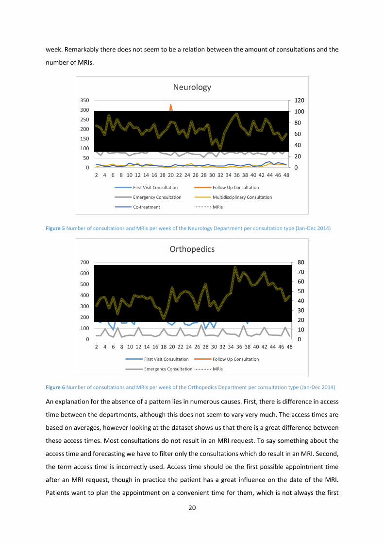
Figure 5 and Figure 6

Figure 6 shows the top two MRI appointment contributors, Neurology and Orthopedics, and the

division of the different types of consultations, as well as the number of MRIs (secondary axis) per

Specialty # Consults # MRIs Share Specialty # Consults # MRIs Share

Radiotherapy 7451 279 4% Urology 17411 215 1%

Cardiology 33090 466 1% Otolaryngology 35346 405 1%

Internal Medicine 43478 342 1% Paediatrics 18314 123 1%

Pulmonology 21277 99 0% Orthopedics 33181 2049 6%

Gastroenterology 16518 394 2% Other Specialists 7120 36 1%

Rheumatology 14712 173 1% Rehabilitation 2763 20 1%

Neurology 24321 2911 12% Cardiothoracic Surgery 1059 6 1%

Surgery 79565 1284 2% Psychiatry 7443 1 0%

Dermatology 17807 1 0% Intensivists 5 10 200%

Ophthalmology 22368 46 0% Radiology 613 0 0%

Neurosurgery 5938 700 12% Oral Surgery 17429 48 0%

Gynecology 29454 89 0% Clinical Neurophysiology 2 2 100%

Plastic Surgery 9458 129 1% Psychology 5410 0 0%

Anesthesiology 3750 146 4% General Practitioners 0 759 0%

Total 475283 10733 2%

0

10

20

30

40

50

60

70

80

0

100

200

300

400

500

600

700

2 4 6 8 10 12 14 16 18 20 22 24 26 28 30 32 34 36 38 40 42 44 46 48

Orthopedics

First Visit Consultation Follow Up Consultation

Emergency Consultation MRIs

20

week. Remarkably there does not seem to be a relation between the amount of consultations and the

number of MRIs.

Figure 5 Number of consultations and MRIs per week of the Neurology Department per consultation type (Jan-Dec 2014)

Figure 6 Number of consultations and MRIs per week of the Orthopedics Department per consultation type (Jan-Dec 2014)

An explanation for the absence of a pattern lies in numerous causes. First, there is difference in access

time between the departments, although this does not seem to vary very much. The access times are

based on averages, however looking at the dataset shows us that there is a great difference between

these access times. Most consultations do not result in an MRI request. To say something about the

access time and forecasting we have to filter only the consultations which do result in an MRI. Second,

the term access time is incorrectly used. Access time should be the first possible appointment time

after an MRI request, though in practice the patient has a great influence on the date of the MRI.

Patients want to plan the appointment on a convenient time for them, which is not always the first

0

20

40

60

80

100

120

0

50

100

150

200

250

300

350

2 4 6 8 10 12 14 16 18 20 22 24 26 28 30 32 34 36 38 40 42 44 46 48

Neurology


Emergency Consultation Multidisciplinary Consultation

Co-treatment MRIs

0

10

20

30

40

50

60

70

80

0

100

200

300

400

500

600

700

2 4 6 8 10 12 14 16 18 20 22 24 26 28 30 32 34 36 38 40 42 44 46 48

Orthopedics


Emergency Consultation MRIs

21

available option. Lastly, there are also MRI requests which are planned well in advance. Most of these

MRIs probably come from Follow up consultations, since they request a checkup MRI for the patient

to monitor the patient's recovery after a period of, say, six months.

With these different sources of noise in the data, it is difficult to forecast the number of patients who

arrive at the diagnostics department for an MRI with the current data.

2.4 Conclusion

The access time of the MRI is exceeding the treeknorm regularly, this is probably the result of the

variation of the number of MRIs between weeks. We compared these number of MRI scans with the

number of consultations, however, no pattern was found. The only conclusion we could draw is that

there is also a lot of variation in the number of consultations. So far, it is not possible to say something

about the forecasting of the number of patients who arrive at the diagnostics department for an MRI.

In Chapter 3 we will do a more extensive data analysis to try to generate the forecasting method to

predict the arrival of patients.

22

3 Extensive Data Analysis

In this chapter we perform an extensive data analysis of the data generated from the outpatient clinic

and the diagnostics department. First we focus on the data of the outpatient clinic, using the number

of consultations per specialty per week per consultation type (Section 3.1). Second we use the data of

the diagnostics department to determine from which specialty and consultation type the MRI has been

requested (Section Fout! Verwijzingsbron niet gevonden.). In Section 3.3 we will perform a correlation

analysis to check if there is a correlation between the number of consultations and the number of MRI

requests per specialty and consultation type. The explanatory factors will be discussed in the Section

3.4.

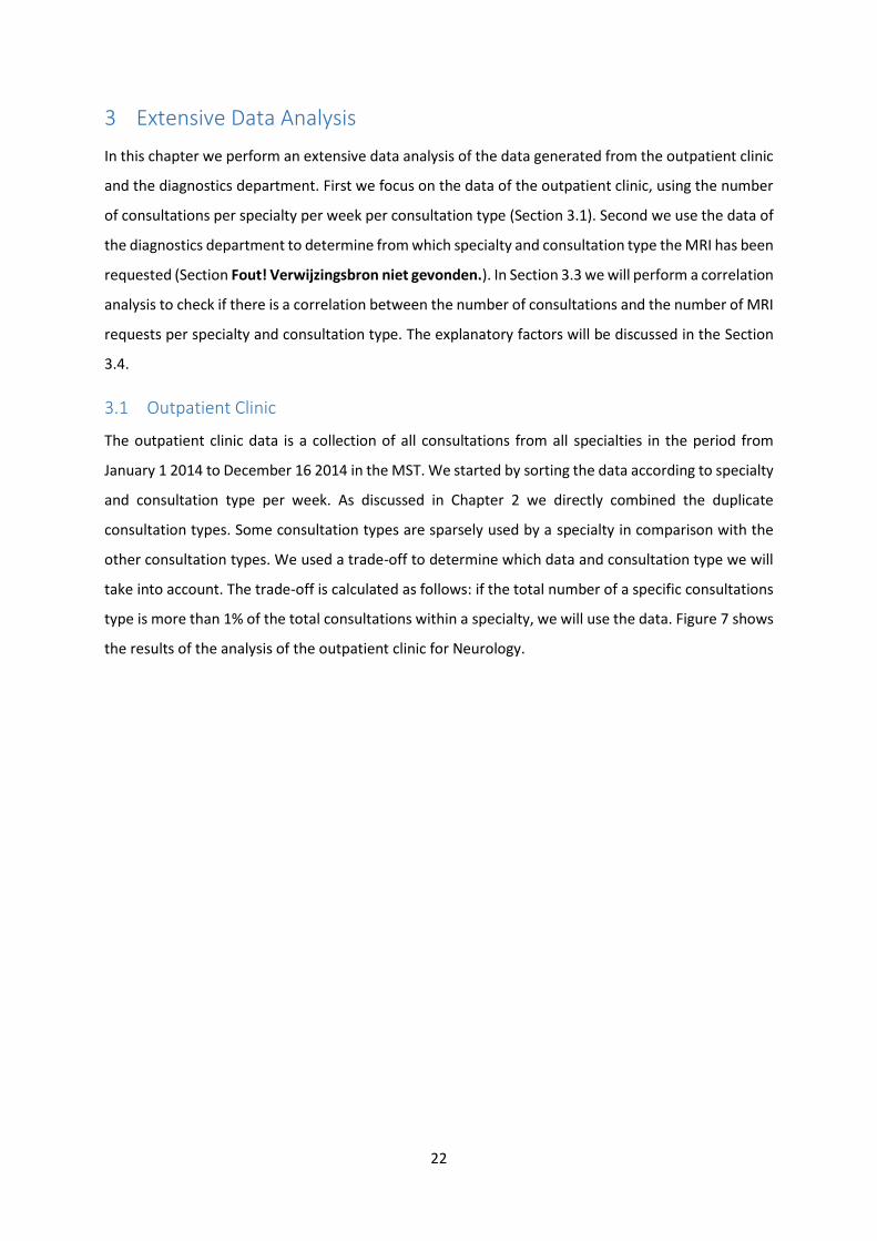
3.1 Outpatient Clinic

The outpatient clinic data is a collection of all consultations from all specialties in the period from

January 1 2014 to December 16 2014 in the MST. We started by sorting the data according to specialty

and consultation type per week. As discussed in Chapter 2 we directly combined the duplicate

consultation types. Some consultation types are sparsely used by a specialty in comparison with the

other consultation types. We used a trade-off to determine which data and consultation type we will

take into account. The trade-off is calculated as follows: if the total number of a specific consultations

type is more than 1% of the total consultations within a specialty, we will use the data. Figure 7 shows

the results of the analysis of the outpatient clinic for Neurology.

23

Figure 7 Number of consultations per week and consultation type of the Neurology Department (Jan-Dec 2014)

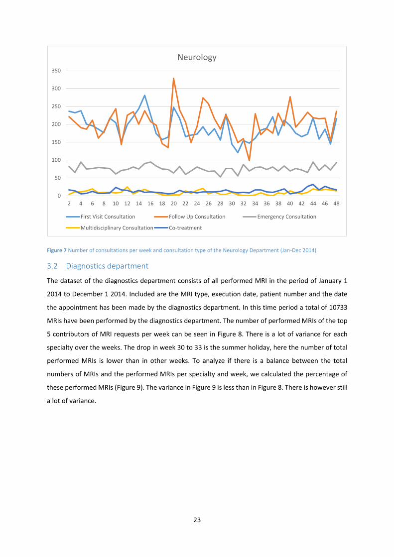
3.2 Diagnostics department

The dataset of the diagnostics department consists of all performed MRI in the period of January 1

2014 to December 1 2014. Included are the MRI type, execution date, patient number and the date

the appointment has been made by the diagnostics department. In this time period a total of 10733

MRIs have been performed by the diagnostics department. The number of performed MRIs of the top

5 contributors of MRI requests per week can be seen in Figure 8. There is a lot of variance for each

specialty over the weeks. The drop in week 30 to 33 is the summer holiday, here the number of total

performed MRIs is lower than in other weeks. To analyze if there is a balance between the total

numbers of MRIs and the performed MRIs per specialty and week, we calculated the percentage of

these performed MRIs (Figure 9). The variance in Figure 9 is less than in Figure 8. There is however still

a lot of variance.

0

50

100

150

200

250

300

350

2 4 6 8 10 12 14 16 18 20 22 24 26 28 30 32 34 36 38 40 42 44 46 48

Neurology

First Visit Consultation Follow Up Consultation Emergency Consultation

Multidisciplinary Consultation Co-treatment

24

Figure 8 Number of performed MRIs per week for the Neurology, Orthopedics, Surgery, Neurosurgery Department and the General Practitioners (Jan-Dec 2014)

0

10

20

30

40

50

60

70

80

90

2 4 6 8 10 12 14 16 18 20 22 24 26 28 30 32 34 36 38 40 42 44 46 48

# M

RIs

Week

Number of performed MRIs per specialty per week

Neurology Orthopedics Surgery General Practitioners Neurosurgery

25

Figure 9 Percentage of performed MRIs per week for the Neurology, Orthopedics, Surgery, Neurosurgery Department and the General Practitioners (Jan-Dec 2014)

We can conclude from Figure 9 that the variance is partly but not completely caused by the total

number of performed MRIs at the diagnostics department. This means that a lot of variance comes

from the outpatient clinics, which we also saw in Figure 7.

3.3 Correlation Analysis

In Section Fout! Verwijzingsbron niet gevonden. we concluded that there might not be a pattern

between the number of consultations and the amount of requested MRIs. A correlation analysis needs

to be done to check if this conclusion is correct. To do a proper correlation analysis we have to make

an overview of the requested MRIs per specialty and consultation type per week. Therefore we need

to know which consultation led to an MRI request.

The datasets cannot be compared with each other since they use different internal operation codes.

For example, the dataset from the diagnostics department shows patient 00030609 with code M3-86,

while the data from the outpatient clinic uses for the same appointment three CTG-codes: 81092,

83190, and 83290. This results in duplicates (Table 4) which we will have to delete. To do this we used

the data of the outpatient clinic and added the column “Appointment made by diagnostics

department”. From the data from the diagnostics department we could fill in the date and time the

0%

5%

10%

15%

20%

25%

30%

35%

40%

2 4 6 8 10 12 14 16 18 20 22 24 26 28 30 32 34 36 38 40 42 44 46 48

Per

cen

tage

to

tal M

RIs

Week

Percentage per specialty of the total performed MRIs per week

Neurology Orthopedics Surgery General Practitioners Neurosurgery

26

appointment was scheduled by the diagnostics department. Subsequently, we sorted the dataset by

patient number. All appointments which have the same patient number and planning date have to be

duplicates and were deleted. A total of 2646 “duplicates” have been removed and 10536 MRI

appointments remain in the dataset.

Table 4 Screen of a duplicate appointment for patient 00030609 with CTG-codes 081092, 083190 and 083290 but only one MRI on 20-11-2013

Now that the duplicates have been removed, we have to find the consultation which led to the

performed MRI. Once we know which consultation was the predecessor of an MRI scan, we also know

what type the consultation was. This is needed to make a forecasting model.

In the period of January 1 2014 to December 1 2014, the MST held 475.000 consultations and had

120.000 unique patients, so every patients had on average 4 consultations in a year. In Section 2.3.1

we discussed that the access time cannot be known for certain, so we cannot use access time as a

method to determine the correct consultation. Since most patients have more than one consultation,

it is not sufficient to take the first consultation before an MRI. It is a good indicator, but some MRI

appointments are made long in advance. To be more certain which consultation led to the MRI request,

we used the dataset of the diagnostics department including the date and time of the planning of the

appointment. This is often not the same date as the actual consultation date, because the

communication in the MST still goes via paper forms and not every request will be scheduled as soon

as possible, so there can be some days between those two dates. If the date of a consultation is before

the MRI, but after the date when the appointment was scheduled, it most probably is the consultation

which led to the MRI request. For these cases (N=1338), we took the last consultation before the date

of scheduling.

Interne Verrichting CodeInterne Verrichting OmsMaand Uitvoerdatum Verr Intern Specialisme Oms AanvrVerr Intern Specialisme Oms UitvVerr Patient CodeWeek Weekdag Hoeveelheid

afspraak

gemaakt

door

radiologie SLEUTEL DUBBELCODE

081092 MRI hersenen - met contrast.5 1-5-2014 NeurologieRadiologie 00021243 18 4 1 7-4-2014 0002124341760 0

081093 MRI hersenen - standaard.2 2-2-2014 NeurologieRadiologie 00024714 5 7 1 29-1-2014 0002471441672 0

081092 MRI hersenen - met contrast.4 28-4-2014 NeurologieRadiologie 00024963 18 1 1 0002496341757 0

089090 MRI heup(en)/ onderste extremiteit(en).9 16-9-2014 OrthopedieRadiologie 00027579 38 2 1 4-9-2014 0002757941898 0

087090 MRI abdomen. 10 17-10-2014 RadiotherapieRadiologie 00027648 42 5 1 10-10-2014 0002764841929 0



089090 MRI heup(en)/ onderste extremiteit(en).7 28-7-2014 Huisartsen Radiologie 00029309 31 1 1 23-6-2014 0002930941848 0

085190 MRI-hart. 10 15-10-2014 CardiologieRadiologie 00029651 42 3 1 3-9-2014 0002965141927 0


081092 MRI hersenen - met contrast.1 7-1-2014 NeurologieRadiologie 00030609 2 2 1 20-11-2013 0003060941646 0

083190 MRI cervicale wervelkolom en/of hals inclusief craniovertebr1 7-1-2014 NeurologieRadiologie 00030609 2 2 1 20-11-2013 0003060941646 1

083290 MRI thoracale wervelkolom.1 7-1-2014 NeurologieRadiologie 00030609 2 2 1 20-11-2013 0003060941646 1


083190 MRI cervicale wervelkolom en/of hals inclusief craniovertebr10 7-10-2014 NeurologieRadiologie 00031882 41 2 1 26-9-2014 0003188241919 1



27

For 365 inpatient clinic consultations, there was not a planning date for the diagnostics department.

This would result in a loss of data, therefore we used an access time based on practice of 2 days. This

is a common access time for MRI requests coming from the inpatient clinic.

Figure 10 Overview of the number of appointments that could be linked

It was not possible to link all the appointments (Figure 10). Out of the 10536 MRI appointments 1449

(13.8%) found no consultation date before the execution date and 457 (4.3%) were MRI requests from

2013. These had to be deleted as well since we did not have those data. 583 appointments were for

some reason not planned by the diagnostics department, these might have been emergency cases. 64

28

appointments had more than one factor, which leads to a total loss of 1449 + 457 + 583 – 64 = 2425

MRIs where we could not say with a certainty which consultation led to those particular MRI requests.

Using the planning date the diagnostics department used (as discussed previously) as a check, resulted

in 1338 cases which had to be recalculated. These cases were all appointments of consultations which

were held later than the date the diagnostics department planned the MRI, which is not possible. That

is why we used the first consultation before the planning date. This resulted in another 246 items of

data loss, due to not enough information about the appointments (consultations which were held in

2013). At the end of the process of cleaning up the 10536 available appointments, we can use 7865

(74.6%) of them for further analyses.

The diagnostics department sometimes combines different MRIs appointments. The 7865 MRI

appointments correspond to 8030 MRI scans. Based on these 8030 MRIs we could calculate the

number of requested MRIs per specialty, per consult type per week. If we focus for example on

Orthopedics we see that in week 4 26 consultations required an MRI (Figure 11). We have to keep in

mind that due to the aforementioned data loss of 25% this probably should be somewhat higher than

26 consultations. Figure 11 shows clearly that there is a high variance in the number of requested MRIs

for Orthopedics, especially for the requests that came from first visit consultation. The variance in

follow up consultations is smaller. This trend is also visible in the other specialties.

Figure 11 Number of requested MRIs coming from the first visit and follow up consultations of the Orthopedics Department (Jan-Dec 2014)

0

5

10

15

20

25

30

35

40

45

50

1 3 5 7 9 11 13 15 17 19 21 23 25 27 29 31 33 35 37 39 41 43 45 47

Nu

mb

er o

f re

qu

este

d M

RIs

Week

Orthopedics


29

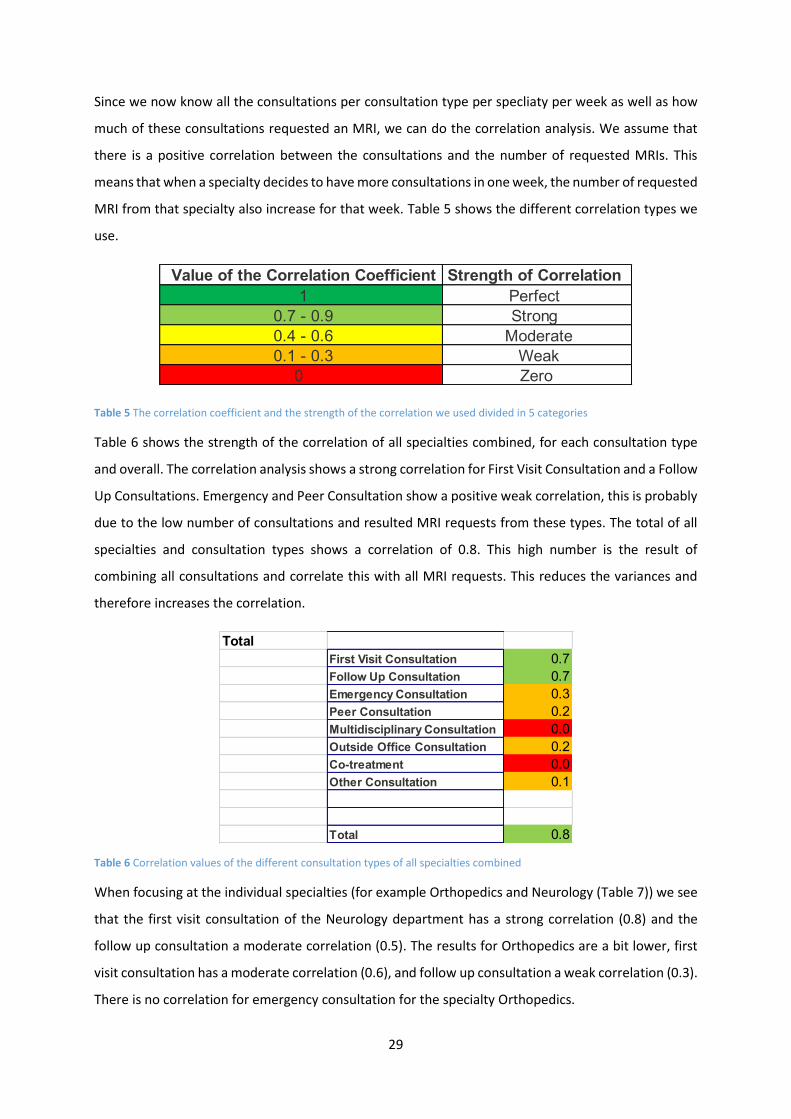
Since we now know all the consultations per consultation type per specliaty per week as well as how

much of these consultations requested an MRI, we can do the correlation analysis. We assume that

there is a positive correlation between the consultations and the number of requested MRIs. This

means that when a specialty decides to have more consultations in one week, the number of requested

MRI from that specialty also increase for that week. Table 5 shows the different correlation types we

use.

Table 5 The correlation coefficient and the strength of the correlation we used divided in 5 categories

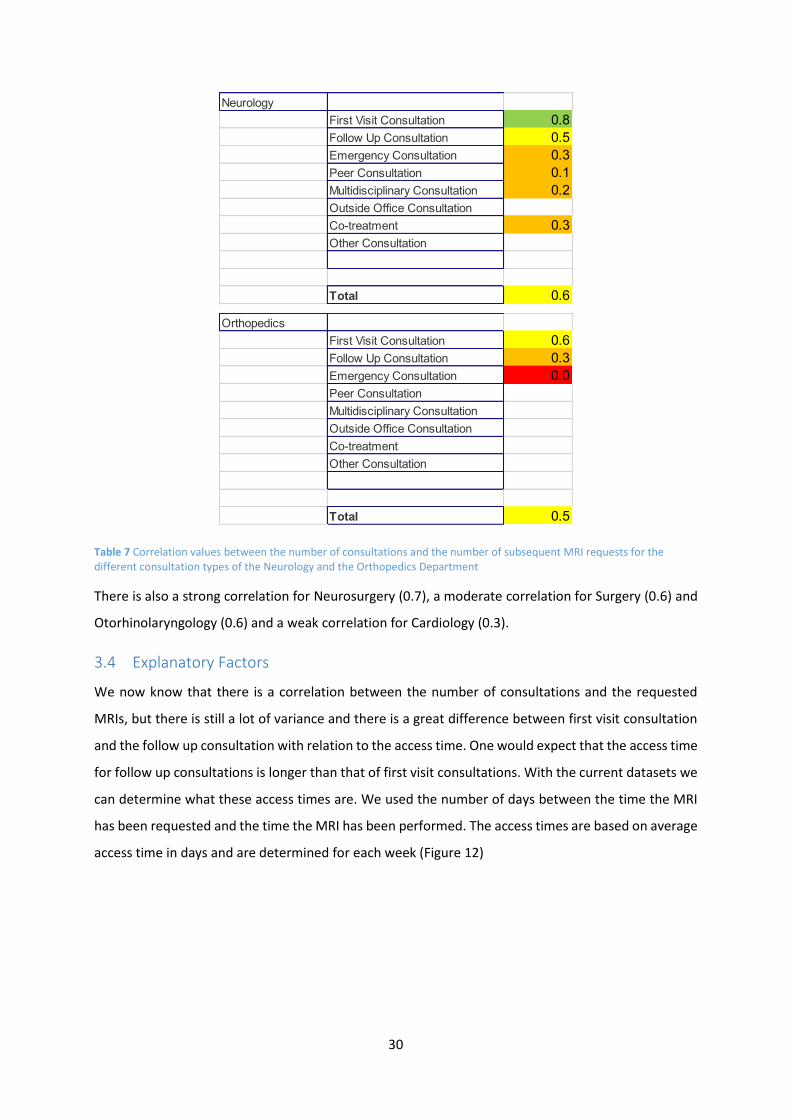
Table 6 shows the strength of the correlation of all specialties combined, for each consultation type

and overall. The correlation analysis shows a strong correlation for First Visit Consultation and a Follow

Up Consultations. Emergency and Peer Consultation show a positive weak correlation, this is probably

due to the low number of consultations and resulted MRI requests from these types. The total of all

specialties and consultation types shows a correlation of 0.8. This high number is the result of

combining all consultations and correlate this with all MRI requests. This reduces the variances and

therefore increases the correlation.

Table 6 Correlation values of the different consultation types of all specialties combined

When focusing at the individual specialties (for example Orthopedics and Neurology (Table 7)) we see

that the first visit consultation of the Neurology department has a strong correlation (0.8) and the

follow up consultation a moderate correlation (0.5). The results for Orthopedics are a bit lower, first

visit consultation has a moderate correlation (0.6), and follow up consultation a weak correlation (0.3).

There is no correlation for emergency consultation for the specialty Orthopedics.

Value of the Correlation Coefficient Strength of Correlation

1 Perfect

0.7 - 0.9 Strong

0.4 - 0.6 Moderate

0.1 - 0.3 Weak

0 Zero

Total

First Visit Consultation 0.7

Follow Up Consultation 0.7

Emergency Consultation 0.3

Peer Consultation 0.2

Multidisciplinary Consultation 0.0

Outside Office Consultation 0.2

Co-treatment 0.0

Other Consultation 0.1

Total 0.8

30

Table 7 Correlation values between the number of consultations and the number of subsequent MRI requests for the different consultation types of the Neurology and the Orthopedics Department

There is also a strong correlation for Neurosurgery (0.7), a moderate correlation for Surgery (0.6) and

Otorhinolaryngology (0.6) and a weak correlation for Cardiology (0.3).

3.4 Explanatory Factors

We now know that there is a correlation between the number of consultations and the requested

MRIs, but there is still a lot of variance and there is a great difference between first visit consultation

and the follow up consultation with relation to the access time. One would expect that the access time

for follow up consultations is longer than that of first visit consultations. With the current datasets we

can determine what these access times are. We used the number of days between the time the MRI

has been requested and the time the MRI has been performed. The access times are based on average

access time in days and are determined for each week (Figure 12)

Neurology




Peer Consultation 0.1

Multidisciplinary Consultation 0.2

Outside Office Consultation

Co-treatment 0.3

Other Consultation

Total 0.6

Orthopedics




Peer Consultation

Multidisciplinary Consultation

Outside Office Consultation

Co-treatment

Other Consultation

Total 0.5

31

Figure 12 Access Time in number of days per week for each consultation type of the Orthopedics Department and all specialties combined (Jan-Dec 2014)

There are great differences in the access times over the weeks. These could be explained by the

phenomenon that when the waiting time of the operation room is high, more surgeons will come to

operate to reduce this waiting time. These surgeons are also the people who take the consultations,

therefore the waiting list for outpatient clinic will grow. This leads to less consultations and, due to the

correlation between them, less MRI requests and lower access times. When the waiting time for the

outpatient clinic is too high, or the waiting time for the OR too small, more specialists will help to

reduce the outpatient clinic waiting list. This will result in more consultations, so more MRI requests

and a higher access time for an MRI.

This effect should be highest with first visit consultations, because most MRI appointments will be

planned as soon as possible. However Figure 12 shows that the variation for the follow up

0

10

20

30

40

50

60

70

80

2 4 6 8 10 12 14 16 18 20 22 24 26 28 30 32 34 36 38 40 42 44 46 48

Nu

mb

er o

f D

ays

Week

Access Time Orthopedics


0

20

40

60

80

100

120

2 4 6 8 10 12 14 16 18 20 22 24 26 28 30 32 34 36 38 40 42 44 46 48

Nu

mb

er o

f d

ays

Week

Access Time of all specialties combined


Emergency Consultation

32

consultations and not first visit consultation is higher. This is due to another cause: the access time is

much more variable because of the fact that some of the MRI appointments are being made far in

advance. These outliers cause for a lot of variance. The effect of the bullwhip effect of the specialist is

still higher in first visit consultations, but less visible because of the outliers from follow up

consultations.

Remarkable is the almost linear decrease from week 30 onwards (Figure 12), which is visible in the

specialty Orthopedics and in all specialties combined. In our research we only use coupled

appointments, so all appointments contain an outpatient clinic consultation and the appointment of

the performed MRI. Our data runs to Dec 2014, which means that at the end of the period only

appointments with a lower access time can occur. It could be that there are consultations with an MRI

appointments in Dec 2014 and beyond, but we do not have these data and therefore cannot calculate

these longer access times.

Figure 13 Percentage of the number of consultations which led to an MRI request per week and consultation type for all specialties combined (Jan-Dec 2014)

Since we know that there is a correlation between the consultations and the requested MRIs from

these consultations, we can analyze if it is possible to use the percentage of the consultations

requesting an MRI as a forecasting value. Figure 13 shows us this percentage for all specialties. This

percentage is very stable over time with a small standard deviation (0.4%). The number of data points

is very high, since all the specialties are combined, and therefore the standard deviation is low.

Focusing on a single specialty, for example Orthopedics, is showing not only a higher percentage, but

0%

1%

1%

2%

2%

3%

3%

4%

4%

5%

2 4 6 8 10 12 14 16 18 20 22 24 26 28 30 32 34 36 38 40 42 44 46 48

Per

cen

tage

Week

Percentage of consultations which request a MRIAll specialties combined

First Visit Consultation Follow Up Consultation Emergency Consultation

33

also a higher standard deviation (3.9% for First Visit Consultation and 1.2% for Follow up Consultation)

(Figure 14).

Figure 14 Percentage of the number of consultations which led to an MRI request per week and consultation type for the specialty Orthopedics (Jan-Dec 2014)

3.5 Conclusions

Extensive data analysis shows us that we can use the number of consultations as an input variable for

the model. There is a strong correlation between the number of consultations and the amount of MRI

requests coming from these consultations. With the use of the ratio of these consultations we could

predict the number of arrivals. Not every specialty has a strong correlation and some specialties have

a higher standard deviation in percentages of consultations requesting an MRI. This has to be kept in

mind when building the model in Chapter 4.

0%

5%

10%

15%

20%

25%

30%

2 4 6 8 10 12 14 16 18 20 22 24 26 28 30 32 34 36 38 40 42 44 46 48

Per

cen

tage

Week

Percentage of Consultations which request a MRI of the specialty Orthopedics


34

4 Forecast Model MRI Demand

In this chapter we build the forecasting model. We start with determining the input values (Section

4.1) of the model. In Section 4.2 we describe the method we used to determine the outcomes and

explain how the model works. The outcomes themselves are discussed in Section 4.3. The validation

of the model will be done in Section 4.4. In Section 4.5 we focus at commonly used forecasting methods

such as the moving average and exponential smoothing method. Finally we end this chapter with a

conclusion in Section 0. A manual of the model can be found in Appendix B – Manual Forecasting

ModelAppendix B – Manual Forecasting Model.

4.1 Input values

The model was developed in Excel because of the high availability of this program in the MST. The

people who have to work with the model (MR-planners) already know how to work with Excel. The

model should be built foolproof. We will use the scheduled number of consultations as input variables,

since we prefer a causal forecast model. The advantage of a causal forecast model is that you can

predict the change in demand in advance, whether a time series forecast method uses previous data

and will therefore lack behind.

The model will be based on six different specialties: Neurology, Orthopedics, Surgery, Neurosurgery,

Cardiology and EMT. These six specialties have the most MRI referrals in the hospital. Together with

the General Practitioners they use 80% of all MRIs. The General Practitioners are excluded of the input

screen (Figure 15) because there is no data available on the number of consultations. The number of

MRI referrals the general practitioners send weekly are known and we use an average of these

numbers as input. This holds as well for the other specialties. The number of generated MRI requests

by the general practitioners are 16 and 44 for the other specialties (the renaming 20%) combined each

week. These values can be found in the “Data” worksheet of the model, which will be explained more

in Section 4.2.

Figure 15 Input screen of our forecasting model

35

The specialties are divided in two different input variables: First visit consultation and follow up

consultation. This is done because we found different percentages of MRI referrals coming from both

consultation types in our research. There is also a clear distinction of these consultations in the data,

so this will result in better forecasting. Every week the new number of consultations has to be entered.

For six weeks the number of consultations for each consultation type and specialty will have to be

noted, whereby week 1 is the current week. These data must be send by the specialties themselves

since the diagnostics department has no access to these data yet. Subsequently the diagnostics

department can fill in all the data and run the model. There are two buttons on the input page: New

Week and Calculate. New Week will shift all weeks one week to the front, so the new values can be

added in for the new week 6. The button Calculate will result in the calculation of the model. Both

buttons will be explained in more detail in Section 4.2. It should not be much work to keep this field

updated, once every week (preferably Monday mornings) the values have to be added. Every specialty

should know the number of consultations for each consultation type.

4.2 Black box

The black box is the working of the model. It calculates with the help of the “Data” worksheet the

number of consultations to the number of expected MRI requests. As discussed in Section 4.1, there

are two buttons on the input page, New Week and Calculate (Figure 15). The button New Week should

be pressed when a new week starts and the diagnostics department wants to add a new week. All

weeks shift up one week which will clear a space for the new data. Besides convenience to fill in the

model, it also stores the last week in the worksheet “Historical Data”. It saves the input of last week

and the corresponding calculated output, as well as the week number (Figure 16).

Figure 16 The input and historical data screen of our forecasting model after pushing the New Week button

Specialisme:

Eerste poli Herhaal Eerste poli Herhaal Eerste poli Herhaal Eerste poli Herhaal Eerste poli Herhaal Eerste poli Herhaal

Aantal Consulten Week 1: 237 222 170 383 476 1267 81 82 197 356 304 630

Week 2: 233 206 154 444 421 1178 72 60 257 541 327 615

Week 3: 238 190 242 551 403 1176 71 72 182 475 292 550

Week 4: 200 186 140 356 459 1076 77 78 194 387 288 524

Week 5: 196 211 88 332 469 1014 66 60 181 466 287 567

Week 6:

KNONeurologie Orthopedie Chirurgie Neurochirurgie Cardiologie


Week 2 237 222 170 383 476 1267 81 82 197 356 304 630 50 33 34 9 6 11 16 44 203

Cardiologie KNOWEEKNUMMER

INPUT: AANTAL CONSULTEN VOORSPELLING: AANTAL MRI'SNeurologie Orthopedie Chirurgie Neurochirurgie Cardiologie KNO

Neurologie Huisartsen Overigen TotaalOrthopedie Chirurgie Neurochirurgie

36

Figure 17 The data screen of our forecasting model

The Calculate button triggers the actual calculation of the model. It uses the input values and uses with

the help of the data analyzed in Chapter 3 to forecast the number of MRI requests for each specialty,

see Eq. 1. 1Our forecasting model consists of three parts:

1. The number of MRI requests from the General Practitioners and other specialties

2. The number of MRI requests coming from FVC and FUC for each specialty

3. The number of MRI requests coming from EC for each specialty

For part 1 we only have constant 𝐶, which is the constant of MRI requests of the General Practitioners

and the other specialties. For part 2 we summarize over the different consultation types 𝑗 and specialty

𝑛 (so in our case 𝑛 = 6). 𝛼𝑖𝑗 is the percentage of consultations which will request an MRI for specialty

𝑖 and consultation type 𝑗 and 𝑋𝑖𝑗𝑡 is the number of consultation of specialty 𝑖 and consultation type 𝑗

in week 𝑡. Part 3 is the most difficult because we do not know exactly the number of emergency

consultations. However we do know the percentage of the emergency consultation out of the total

consultations: 𝛾𝑖. We estimate the total consultations with (𝑋𝑖1𝑡+𝑋𝑖2𝑡

1−𝛾𝑖) and by multiplying this with 𝛾𝑖

we have an estimation of the number of emergency consultations. 𝛽𝑖 is the percentage of consultation

which will request a MRI for specialty 𝑖. Adding these 3 parts you get 𝑌𝑡 which is the forecasting of the

number of MRI request in week 𝑡.

𝑌𝑡 = 𝐶 + ∑ ∑(𝛼𝑖𝑗 ∗ 𝑋𝑖𝑗𝑡)

2

𝑗=1

𝑛

𝑖=1

+ ∑ 𝛽𝑖 ∗ 𝛾𝑖 ∗ (𝑋𝑖1𝑡 + 𝑋𝑖2𝑡

1 − 𝛾𝑖)

𝑛

𝑖=1

1

The calculation process consists of five steps.

Specialisme Eerste poli Herhaal Spoed

1 Neurologie 14.6% 4.5% 6%

2 Orthopedie 15.0% 2.0% 0%

3 Chirurgie 1.0% 2.0% 1%

4 Neurochirurgie 6.5% 5.1% 3%

5 Cardiologie 1.1% 0.9% 1%

6 KNO 0.6% 1.4% 0%

8 Huisartsen 16

9 Overigen 44

Percentage MRI's

37

Step 1: Clear the Previous Forecasting.

First the “Output” worksheet will be cleared of the previous prediction. The first week has been copied

to the “Historical Data” worksheet by the New Week button. The whole outcome will be cleared, since

it might be possible that more input values have been updated.

Step 2: Add the number of MRIs for the general practitioners and the other specialties (part 1).

The constant values 𝐶 are defined in the “Data” worksheet (Figure 17) and are being added to the

“Output” worksheet for each week. These values can be changed when necessary in the “Data”

worksheet.

Step 3: Calculate the number of requested MRI for first visit consultation and follow up consultation

(part 2).

We can calculate the number of requested MRIs by using part 2 of Equation 11. The percentages 𝛼𝑖𝑗

are the average percentages taken over 46 weeks of our historical data (Jan-Dec 2014) of specialty 𝑖

and can be found in the “Data” worksheet (Figure 17). Multiplying these values with the number of

consultations 𝑋𝑖𝑗𝑡 for each consultation type 𝑗 results is a good estimation of the number of requested

MRIs.

Step 4: Estimate the number of Emergency MRI requests (part 3).

Using part 3 of Equation 1 will give us the number of MRI requests coming from emergency

consultations. The percentages 𝛽𝑖 and 𝛾𝑖 are the average percentages taken over 46 weeks of our

historical data (Jan-Dec 2014) of specialty 𝑖 and can be found in the “Data” worksheet (Figure 17).

Step 5: Calculate the total amount of estimated MRI requests.

The values of the estimated first visit, follow up and emergency consultation are added as the total

estimated MRI requests per specialty per week in the “Output” worksheet. The total amount of

estimated MRI request per week are all these values from every specialty as well as the values of the

general practitioner and the remained specialties. See Section 4.3 for more information about the

Output values and what they mean.

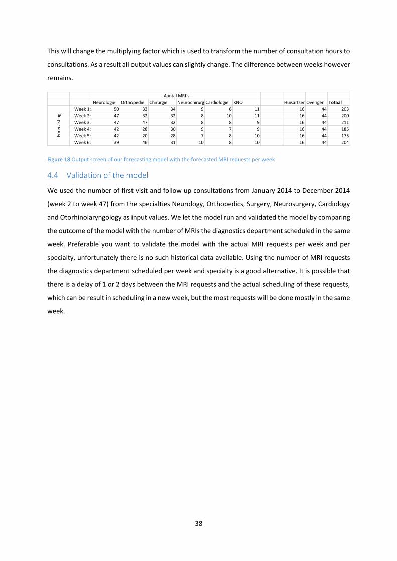
4.3 Output

The “Output” worksheet is the summery of the forecasting (Figure 18) made by the model. The total

amount per each specialty per week can be seen as well as the overall predicted amount of MRI

requests. The forecasting is done for the next six weeks and the diagnostics department can use this

information for the allocation of personnel and patients. Every week new input values will be added.

38

This will change the multiplying factor which is used to transform the number of consultation hours to

consultations. As a result all output values can slightly change. The difference between weeks however

remains.

Figure 18 Output screen of our forecasting model with the forecasted MRI requests per week

4.4 Validation of the model

We used the number of first visit and follow up consultations from January 2014 to December 2014

(week 2 to week 47) from the specialties Neurology, Orthopedics, Surgery, Neurosurgery, Cardiology

and Otorhinolaryngology as input values. We let the model run and validated the model by comparing

the outcome of the model with the number of MRIs the diagnostics department scheduled in the same

week. Preferable you want to validate the model with the actual MRI requests per week and per

specialty, unfortunately there is no such historical data available. Using the number of MRI requests

the diagnostics department scheduled per week and specialty is a good alternative. It is possible that

there is a delay of 1 or 2 days between the MRI requests and the actual scheduling of these requests,

which can be result in scheduling in a new week, but the most requests will be done mostly in the same

week.

Neurologie Orthopedie Chirurgie NeurochirurgieCardiologie KNO Huisartsen Overigen Totaal

Week 1: 50 33 34 9 6 11 16 44 203

Week 2: 47 32 32 8 10 11 16 44 200

Week 3: 47 47 32 8 8 9 16 44 211

Week 4: 42 28 30 9 7 9 16 44 185

Week 5: 42 20 28 7 8 10 16 44 175

Week 6: 39 46 31 10 8 10 16 44 204

Fore

cast

ing

Aantal MRI's

39

Figure 19 Number of forecasted and real MRI requests per week for 45 weeks (Jan-Dec 2014)

The results of the forecasting and the real outcomes are plotted in Figure 19. We calculated the Mean

Absolute Percentage Error (MAPE) (see Eq. 22) and did a correlation analysis and found a MAPE of

10.2% and a correlation of 0.6. The MAPE gives insight in the forecasting power and is the average

percentage of the difference between the forecasting and the real outcomes. All calculations and

comparison are done on the total outcome of MRIs and not per individual specialty. This is done

because the diagnostics department is only interested in these values. A MAPE of 10.2% means that

our model has on average 10.2% error compared to the real outcomes.

𝑀𝐴𝑃𝐸 = [(1

𝑛) ∑|𝑒𝑖 𝐷𝑖⁄ |

𝑛

𝑖=1

] ∗ 100 2

Focusing on the individual specialties shows us that we underrate and overrate some of the specialties.

Table 8 shows us the error between the average forecasted value and the average real outcomes as

well as the correction we would need to improve the model. Especially Neurology, Neurosurgery and

Cardiology are underrated. The reason for this behavior could be found in the 25% data loss we found

in our data, apparently these specialties had some consultations in the data we lost. Another

explanation could be that these specialties generate MRIs from other consultations than first visit,

follow up or emergency. Our research indicates that this would be unlikely though.

0

50

100

150

200

250

300

MR

Is

Weeks

Number of MRI requests per week

Forecasting Outcome

40

Table 8 Difference of the average forecasted and the real MRI requests, including the correction needed to improve the model (Jan-Dec 2014)

After running the model with the new corrected percentages, we found a MAPE of 9.9%, this is slightly

better than our previous configuration. The last step we can use to improve the model is to check what

the number of MRI requests is of the other remaining specialties. At this moment this value is still 44.

By decreasing this value to 34 MRIs per week, we can improve the model to a MAPE of 9.2% while

keeping the correlation at 0.6. Figure 20 is a representation of our improved forecasting model and

the real outcome of the requested MRIs per week.

Figure 20 Number of forecasted and real MRI requests per week for 45 weeks using the improved forecasting model (Jan-Dec 2014)

4.5 Other Forecasting Methods

The forecasting model we use is based on scheduled future data, there are however also other

forecasting methods who use historical data. This section will compare our forecasting model with

other forecasting methods such as the Moving Average (Section 4.5.1) and Exponential Smoothing

Average

Forecasted

Value

Average

Real

Outcome

Difference

Correction

in

Percentage

Neurology 41 54 13 33%

Orthopedics 37 39 2 6%

Surgery 25 24 -1 -5%

Neurosurgery 7 13 6 90%

Cardiology 7 9 2 36%

Otorhinolaryngology 8 8 -1 -7%

0

50

100

150

200

250

300

Nu

mb

er o

f M

RI r

eqeu

st

Number of MRI requests per week

Improved Forecasting Outcome

41

(Section 4.5.2) (Simchi-Levi, Kaminsky, & Simchi-Levi, 2009). These methods are Time Series Methods;

they require no information other than the past values of the variable being predicted (Nahmias,

1997). The data we use is from Jan-Dec 2014 (week 2 to week 47) and for each method we will

determine the MAPE and the Correlation. We compare these methods with our own model in Section

0 and based on these comparison we improve our model in Section 4.5.4.

4.5.1 Moving Average

The moving average method is a forecasting method that uses the average of the last 𝑁 weeks as a

forecasting (Eq. 3). The simplest moving average method is using a 𝑁 of 1, this is also called Naïve

Forecasting (Nahmias, 1997) (Eq. 4). We calculated the forecast error and correlation of the moving

average method using a 𝑁 of 1 to 10, see Table 9. The moving average of the previous 3 weeks is the

best forecast method (Figure 21), with a MAPE of 8.1% and a correlation of 0.67. Forecasting with a

small 𝑁 follows the demand best, the downside of the moving average is that you can only forecast

over week 𝑡 > 𝑁.

𝐹𝑡 = (

1

𝑁) ∑ 𝐷𝑖

𝑡−1

𝑖=𝑡−𝑁

3

𝐹𝑡 = 𝐷𝑡−1 4

42

Figure 21 Number of forecasted MRI requests using the Moving Average Method (N = 1, 2, 3, 4 and 5) and the actual Demand (Jan-Dec 2014)

Table 9 Mean Average Percentage Error and Correlation of the Moving Average method with an N of 1 to 10 (Jan-Dec 2014)

0

50

100

150

200

250

300

1 2 3 4 5 6 7 8 9 10 11 12 13 14 15 16 17 18 19 20 21 22 23 24 25 26 27 28 29 30 31 32 33 34 35 36 37 38 39 40 41 42 43 44 45 46

#MR

Is

Weeks

Moving Average Method

Demand Moving Average 1 Moving Average 2 Moving Average 3 Moving Average 4 Moving Average 5

MA 1 MA 2 MA 3 MA 4 MA 5 MA 6 MA 7 MA 8 MA 9 MA 10

MAPE 9,6% 8,3% 8,1% 8,6% 8,4% 8,9% 9,4% 10,0% 10,6% 10,8%

Correlation 0,65 0,69 0,67 0,62 0,63 0,59 0,53 0,46 0,35 0,30

43

4.5.2 Exponential Smoothing

Figure 22 Number of forecasted MRI requests using the Exponential Smoothing Method (alpha 0.35) and the actual Demand (Jan-Dec 2014)

The second forecasting method we use is the exponential smoothing method. This method can be

defined as: The forecast in any period 𝑡 is the forecast in period 𝑡 − 1 minus some fraction of the

observed forecast error in period 𝑡 − 1, Eq. 5 (Nahmias, 1997). We calculated the forecast error and

correlation of the exponential smoothing method, using an alpha of 0.1 to 1.0, see Table 10. We used

the solver in Excel to find an even better alpha by minimizing the MAPE. The best alpha for forecasting

the MRI requests is 𝛼 = 0.35 (Figure 22), it has a MAPE of 7.8% and a correlation of 0.72.

𝐹𝑡 = 𝐹𝑡−1 − 𝛼(𝐹𝑡−1 − 𝐷𝑡−1), 0 < 𝛼 ≤ 1 5

Table 10 Mean Average Percentage Error and Correlation of the Exponential Smoothing method with an alpha of 0.1 to 1.0 (Jan-Dec 2014)

0

50

100

150

200

250

300

2 4 6 8 10 12 14 16 18 20 22 24 26 28 30 32 34 36 38 40 42 44 46

#MR

Is

Week

Exponential Smoothing Method

Demand Exponential Smoothing 0.35

EXP 0.1 EXP 0.2 EXP 0.3 EXP 0.4 EXP 0.5 EXP 0.6 EXP 0.7 EXP 0.8 EXP 0.9 EXP 1.0

MAPE 11,2% 8,9% 8,1% 7,9% 8,0% 8,2% 8,5% 8,8% 9,1% 9,6%

Correlation 0,60 0,68 0,71 0,72 0,72 0,71 0,70 0,69 0,67 0,65

44

4.5.3 Comparison

The Exponential Smoothing Method with an alpha of 0.35 has the best results of all Time Series

Methods we analyzed. It preforms much better than our forecasting method which has a forecast error

of 9.2% instead of 7.8% and a correlation of 0.6 instead of 0.7 instead. The difference of the two

forecasting methods is the data the forecasting method use. For the exponential smoothing method it

is the previous demand and forecast, for our own model it is the scheduled number of consultations.

This can also be seen in Figure 23, the exponential smoothing method is smoother and follows the

demand better than our own model and resulting in a better forecasting error and correlation.

Figure 23 Comparison the requested MRIs for the Exponential Smoothing (alpha 0.35) and our Forecasting Model with the Demand (Jan-Dec 2014)

4.5.4 Improving current model

The Exponential Smoothing method forecasts better than our own model, therefore we will combine

the time series methods with our current causal forecasting method to see if this combination will

improve its forecasting ability (Carpenter et al., 2011), see Eq. 7. The best qualities of our causal

forecasting method is the ability to predict an incremental in- or decrease of the number of requested

MRIs. Therefore part 1 of the equation will be the forecast of the causal model, 𝑌𝑡. For strong qualities

of the time series methods is the ability to correct the forecast when the demand is higher of lower

than predicted. The second part of the equation is a combination of the exponential smoothing and

the moving average. For the exponential smoothing we used the difference of the previous forecast

by the causal forecast model and the actual demand, see Figure 24. With this model we found an

optimal alpha of 0.35, a MAPE of 8.8% and a correlation of 0.66.

𝐹𝑡 = 𝑌𝑡 + 𝛼 ∗ (𝑌𝑖 − 𝐷𝑖) 6

0

50

100

150

200

250

300

1 3 5 7 9 11 13 15 17 19 21 23 25 27 29 31 33 35 37 39 41 43 45

#MR

Is

Week

Forecasting and Demand of the requested MRIs

Demand Exponential Smoothing 0.35 Our Model

45

Figure 24 Demand and Forecasting of requested MRIs per week using the previous and its improved forecasting method (exponential smoothing) (Jan-Dec 2014)

This could be even better improved if we also used a moving average part (𝑁 in Eq. 7), because of the

high variation in the forecast. Using an average will reduce this variation. Figure 25 is an overview of

the possible MAPE when using a different 𝑁 and 𝛼. Remarkable is the shape of the figure, for each

moving average the shape is what you would expect. Starting with a MAPE that will decrease when

alpha increases till it reaches its optimum, which then increases again. You would also expect this

behavior when increasing 𝑁 while using the same alpha. Figure 25 however shows us that the moving

average 4 has an higher MAPE that 𝑁 = 3 or 𝑁 = 5. Apparently using the average difference in the

previous demand and the forecast of the last 4 periods differs more with the actual demand than when

using the last 3 or 5 periods.

Using a Moving Average of 𝑁 of 5 proved to have the best results in combination with an alpha of

0.717. With this combination of both our causal forecast model, the exponential smoothing part and

the moving average part we found an optimal a MAPE of 8.0% and a correlation of 0.717, see Figure

26.

𝐹𝑡 = 𝑌𝑡 + 𝛼 ∗ ((1

𝑁) ∑ (𝑌𝑖 − 𝐷𝑖)

𝑡−1

𝑖=𝑡−𝑁

) 7

0

50

100

150

200

250

300

1 3 5 7 9 11 13 15 17 19 21 23 25 27 29 31 33 35 37 39 41 43 45

#MIR

s

Weeks

Forecasting of number of Requested MRIs using current and improved model

Demand Forecasting Model Improved Forecasting Model (Exp Sm)

46

Figure 25 Summary of the Mean Average Percentage Error of the improved forecasting method using alpha 0.1 to 1 and the moving average of 1 to 10 (Jan-Dec 2014)

Figure 26 Demand and Forecasting of requested MRIs per week using the previous and its improved forecasting method (exponential smoothing and moving average (N=5)) (Jan-Dec 2014)

0.1

0.3

0.5

0.7

0.9

8,00%

8,25%

8,50%

8,75%

9,00%

9,25%

9,50%

9,75%

10,00%

10,25%

10,50%

Exp

on

en

tial

Sm

oo

thin

g (a

lph

a)

MA

PE

Moving Average (N)

MAPE of forecasting with the use of Exponential Smooting and Moving Average

0

50

100

150

200

250

300

1 3 5 7 9 11 13 15 17 19 21 23 25 27 29 31 33 35 37 39 41 43 45

#MR

Is

Weeks

Forecasting of requested MRIs using improved forecasting method (Exponential Smoothing and Moving Average)

Demand Forecasting Model Improved Forecasting Model (Exp Sm + MA 5)

47

4.6 Conclusion

The Exponential smoothing method preforms slightly better than our improved model (Table 11), but

we still recommend the diagnostic department of the MST to use our own model. The most valuable

information for the diagnostic department is not the actual number of MRIs, but to see if there will be

a change in demand. When using only the exponential smoothing model, you will detect this change

after it happens, since it uses historical data. With our improved model you can see this coming on

forehand.

Table 11 Overview of the MAPE and Correlation of all forecasting methods we used

We performed a correlation analysis of the demand 𝐷𝑡 – 𝐷𝑡−1 and the forecast 𝐹𝑡 − 𝐹𝑡−1, for the

exponential smoothing and our improved forecasting model and found out that there is negative

moderate correlation for the exponential smoothing (-0.5) and a weak correlation for our model (0.3).

In fact for 69% of the cases our model will forecast correct whether it will be a positive or negative

change compared to the previous week, while the exponential smoothing method only forecasts

correctly for 27% of the times, see Figure 27.

Figure 27 The difference in MRI requests for each week t and week t-1 for the Demand and our Forecasting Model (Jan-Dec 2014)

The forecasting model will be used by the diagnostic department to predict the number of MRI

requests per week and specialty. The diagnostics department will use this to see on forehand how

much referrals they can expect for the coming six weeks. This information can be used to decide to

open the MRI in evenings or weekends when more MRIs requests are to be expected. The planning of

Our Model EXP 0.35 MA 3 Model + EXP 0.35 Model + EXP 0.72 + MA 5

MAPE 9,1% 7,8% 8,1% 8,8% 8,0%

Correlation 0,60 0,72 0,67 0,66 0,72

-80

-60

-40

-20

0

20

40

60

2 3 4 5 6 7 8 9 10 11 12 13 14 15 16 17 18 19 20 21 22 23 24 25 26 27 28 29 30 31 32 33 34 35 36 37 38 39 40 41 42 43 44 45 46

#MR

Is

Week

Difference in MRIs compared to last week

Difference in Demand Improved Forecasting Model (ES + MA) Exponential Smoothing 0.35

48

personnel and patients can be changed. On quiet weeks the diagnostic department can decide to have

less personnel on duty. This will lead to a more stable access time for the radiology, which is beneficial

for all departments that rely on diagnostics.

Another possibility to use the model is to reserve certain blocks for specialties. The scheduling of

patients at the diagnostic department is done in blocks as discussed in Section 2.2.2. With this

information the radiology department can decide to have an extra MRI block for the neurology

department, when demand for this specialty is higher.

Finally the model can also function as a feedback tool to the different departments by showing the

departments the effect of their way of scheduling their consultations. It can be used as a bargaining

position to prevent much variation in the arrival pattern of the patients, which is preferable by the

diagnostic department by adding or removing MRI blocks and by the department in question.

49

5 Conclusion

In our problem formulation we explained the current situation of the diagnostics department. There

is no insight in the arrival of patients from the outpatient clinics to the diagnostics department who

need an MRI. In addition, there is great variation in the number of patients that arrive from each

specialty. This leads to high access times for the diagnostics department and therefore high throughput

times for patients. This led to our following research questions:

1 What does the current care pathway for patients who arrive at the outpatient clinic and

need an MRI at the diagnostics department look like?

In the MST there is a total of 43 different specialties (69 including subspecialties). Most specialties have

outpatient clinics and in these outpatient clinics patients arrive for a consultation. There are eight

different consultations types: First visit consultation, follow up consultation, emergency consultation,

peer consultation, multidisciplinary consultation, outside office consultations, co-treatment, and other

consultations. First visit consultation and follow up consultations are the consultations mainly used in

the outpatient clinic. All consultation types can result in an MRI request.

The seven biggest MRI contributors are Neurology, Orthopedics, General Practitioner, Surgery,

Neurosurgery, Cardiology and Otorhinolaryngology. Together they request 80% of all MRIs. The

referral for an MRI arrives to the radiology department via a paper form, possibly a few days after the

consultation of the patient. The radiology department has divided MRI slots per specialty. Based on

urgency and convenience of the patient, an MRI appointment will be made. This results in certain an

access time for the diagnostics department that varies over the time, exceeding the 'treeknorm' of 4

weeks 25% of the time (in the time July 2013 to May 2014). This results in a longer throughput time

for the patient. So far, there has been no relation found between the number of consultations and the

number of performed MRIs.

2 Is there a correlation between the different consultations and the requested MRIs?

A strong correlation (0.9) is found between the consultations and the requested MRIs, though not

every consultation type has a strong correlation. Emergency consultation and peer consultation have

a moderate correlation with the number of requested MRIs and multidisciplinary consultation, outside

office consultations, co-treatment, and other consultations have a weak correlation.

Focusing on the individual specialties results in lower values for consultations. The highest MRI-request

contributors still have a strong correlation to the number of requested MRIs: Neurology (0.8),

Orthopedics (0.7), Surgery (0.8) and Neurosurgery (0.7). Cardiology (0.5) and Otorhinolaryngology (0.7)

have a moderate correlation. The correlation for other specialties is lower, these are however not

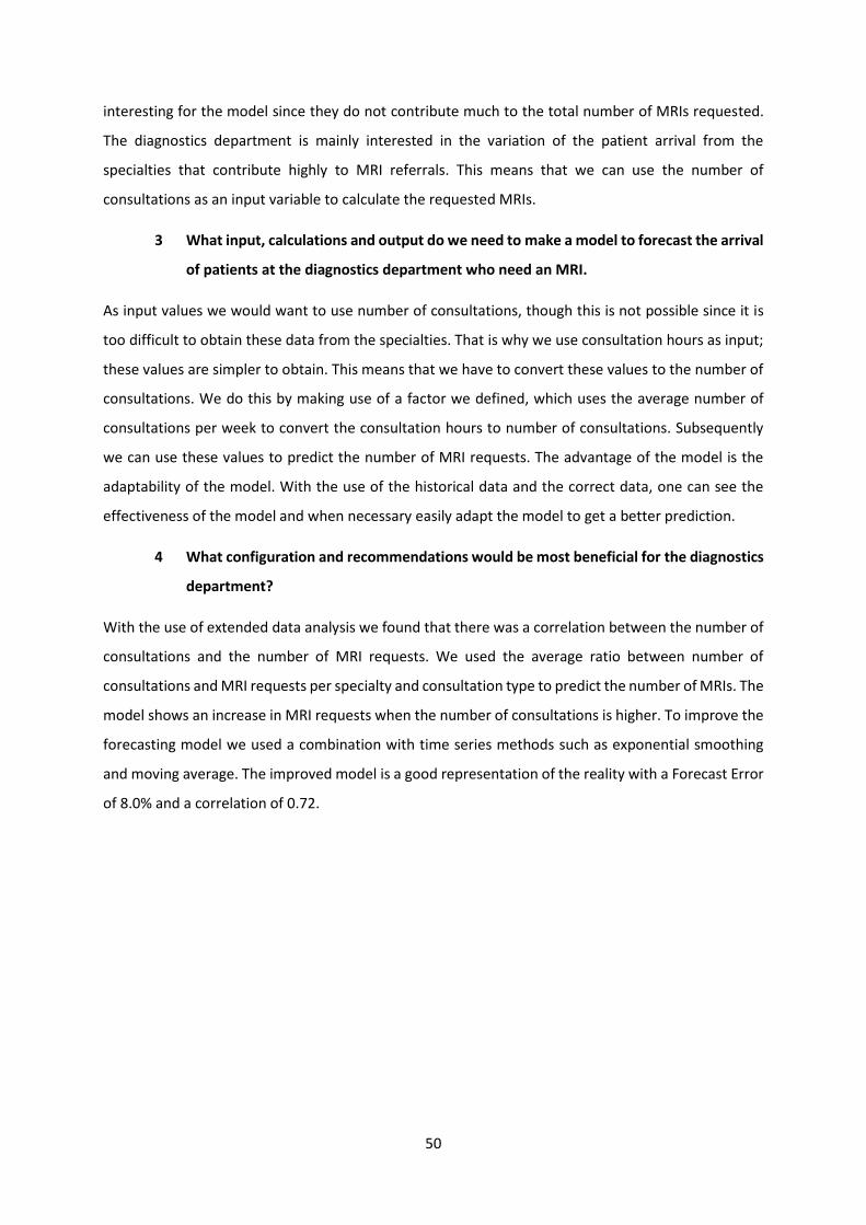
50

interesting for the model since they do not contribute much to the total number of MRIs requested.

The diagnostics department is mainly interested in the variation of the patient arrival from the

specialties that contribute highly to MRI referrals. This means that we can use the number of

consultations as an input variable to calculate the requested MRIs.

3 What input, calculations and output do we need to make a model to forecast the arrival

of patients at the diagnostics department who need an MRI.

As input values we would want to use number of consultations, though this is not possible since it is

too difficult to obtain these data from the specialties. That is why we use consultation hours as input;

these values are simpler to obtain. This means that we have to convert these values to the number of

consultations. We do this by making use of a factor we defined, which uses the average number of

consultations per week to convert the consultation hours to number of consultations. Subsequently

we can use these values to predict the number of MRI requests. The advantage of the model is the

adaptability of the model. With the use of the historical data and the correct data, one can see the

effectiveness of the model and when necessary easily adapt the model to get a better prediction.

4 What configuration and recommendations would be most beneficial for the diagnostics

department?

With the use of extended data analysis we found that there was a correlation between the number of

consultations and the number of MRI requests. We used the average ratio between number of

consultations and MRI requests per specialty and consultation type to predict the number of MRIs. The

model shows an increase in MRI requests when the number of consultations is higher. To improve the

forecasting model we used a combination with time series methods such as exponential smoothing

and moving average. The improved model is a good representation of the reality with a Forecast Error

of 8.0% and a correlation of 0.72.

51

6 Discussion and Recommendations

This chapter will be the discussion of our research and some recommendation for the diagnostics

department to use the model.

We used the historical data from January 2014 to December 2014, which is not a very wide range. Our

extended data analysis shows that there is a correlation between the number of consultations and the

number of MRI requests. The correlation is based on linked appointments. 25% of the data could not

be linked to an appointment and therefore could not be used. The main reason for this data loss is

because of the small data range. Consultations in 2013 and MRI requests for December 2014 and

beyond resulted in data loss. This probably effects follow up consultations the most, since they have a

large amount of MRI requests over a longer period of time. Validating the model showed the same

results; the percentages for neurology, neurosurgery and cardiology were too low and had to be

adjusted to get better results. This correction is however affecting the total number of consultations

and not the individual consultation type.

There are thirteen different types of consultations that are based on the Internal Operation Codes the

MST uses. For convenience we combined these consultations into eight different consultation types.

In the model we only use first visit, follow up and emergency consultation. These are the most

important and most used consultation types, but there are also some MRI requests coming from the

other consultation types. It could therefore mean that we underestimate the number of requested

MRIs. Systematic underestimation will be corrected by the exponential smoothing and moving average

part of the method, but changing the base values is still recommended.

It is not known where the MRI requests come from and when they were requested. For the validation

of the model we used the date the diagnostics department scheduled the MRI. This is however not

accurate, it is possible that there is a delay of one or two days between the MRI request and the

scheduling of this MRI. We recommend the MST to keep track of these data and use it as input values

for our model. The model can still function without these data, but it will decrease its forecasting

power. Furthermore we recommend to validate the model after a period of time with the real MRI

historical request data.

At this moment it is not possible for the diagnostics department to get an overview of the number of

consultations per consultation type for the six specialties we used in our model. This means that the

diagnostics department is depending on the willingness of the specialties to provide accurate data for

the model. We highly recommend the diagnostics department to get access to these data to provide

the model with accurate data.

52

The model we built is a good estimator of the expected MRI requests, however due to the above

mentioned issues it has to be tested before it can be used as a functional tool for the diagnostics

department. Therefore we recommend the MST not to implement this model immediately, but assess

its forecasting strength during a 6 month shadow run. An implementation manual can be found in

Appendix A – Implementation of the forecasting ModelAppendix A – Implementation of the forecasting

Model.

The MST has indicated that when this model is a success, it is interested in using the same method to

forecast the CT requests and other applications. Our model and research is highly adaptable and can

be used when implementing a forecasting model for these other applications. The data of the number

of consultations remain the same, so the only thing the MST needs to do is link the appointments to

the CT requests, following the same steps we used in our research. The values they find can be used in

the same model.

53

References

Busse, R., Geissler, A., Aaviksoo, A., Cots, F., Hakkinen, U., Kobel, C., … Quentin, W. (2013). Diagnosis related groups in Europe: moving towards transparency, efficiency, and quality in hospitals? Bmj (Vol. 346). http://doi.org/10.1136/bmj.f3197

Carpenter, A. P., Leemis, L. M., Papir, A. S., Phillips, D. J., & Phillips, G. S. (2011). Managing magnetic resonance imaging machines: Support tools for scheduling and planning. Health Care Management Science, 14(2), 158–173. http://doi.org/10.1007/s10729-011-9153-z

Gartner, D., & Kolisch, R. (2014). Scheduling the hospital-wide flow of elective patients. European Journal of Operational Research, 233(3), 689–699. http://doi.org/10.1016/j.ejor.2013.08.026

Godin, P., & Wang, C. (2010). Agent-based outpatient scheduling for diagnostic services. Conference Proceedings - IEEE International Conference on Systems, Man and Cybernetics, 1851–1856. http://doi.org/10.1109/ICSMC.2010.5642281

Green, L. V., Savin, S., & Wang, B. (2006). Managing Patient Service in a Diagnostic Medical Facility. Operations Research, 54(1), 11–25. http://doi.org/10.1287/opre.1060.0242

Koenderink, M. (2010). Improving service delivery of the MR department of MST. University of Twente.

Medisch Spectrum Twente. (2012). Jaarimpressie 2012. Enschede. Retrieved from http://www.mst.nl/onzeorganisatie/

Medisch Spectrum Twente. (2013). Bestuursverslag 2012.

Medisch Spectrum Twente. (2014). Toegangstijden en wachttijden. Enschede.

Nahmias, S. (1997). Forecasting. In R. T. Hercher (Ed.), Production and Operations Analysis (3th ed., pp. 59–119). Tom Casson.

Nederlandse Zorgautoriteit. (2011a). Prestaties en tarieven medisch specialistische zorg.

Nederlandse Zorgautoriteit. (2011b). Regeling verplichte publicatie wachttijden somatische zorg.

Ooms, R. (2014). BALANCING THE PATIENT FLOW BETWEEN THE ORTHOPAEDIC OUTPATIENT CLINIC AND THE OPERATING ROOM. University of Twente.

Simchi-Levi, Kaminsky, & Simchi-Levi. (2009). Designing and Managing the Supply Chain: Concepts, Strategies and Case Studies (3th ed.). McGraw-Hill International Edition.

Van Houdenhoven, M. (2007). Healthcare logistics: The art of balance. In Healthcare logistics: The art of balance (p. 12).

Van Oosterom, A., & Oostendorp, T. F. (2008). Medische fysica.

vergelijken-zorgverzekering.net. (n.d.). Treeknorm. Retrieved June 22, 2015, from http://www.vergelijken-zorgverzekering.net/treeknorm

54

Appendix A – Implementation of the forecasting Model

The following steps are designed for the diagnostics department to use this model efficiently into the

daily use. We recommend to use this model in a shadow run first.

Step 1: Involve the different specialties which are going to deliver the input values.

The six specialties have to be involved into the beginning of the process. It is important to let them

understand the value of this model to their department: shorter access times for patients in need of

an MRI. This can be achieved with minimal effort, they only have to provide data to the diagnostics

department once a week. (If the diagnostics department can get direct access to these data, the effort

for the specialties will become nonexistent.)

Step 2: Acquire the input data for six weeks in advance.

In order to start the model, the diagnostics department needs to have 6 weeks of input values. This is

the “warm up period” of the model. You can start with only one specialty involved, but more are

preferable since this indicates the working of the whole model instead of the prediction of one

specialty.

Step 3: Run the model for the first time.

Once you have the data for the first six weeks, the model can be used. You now have a forecast for the

number of MRI requests for the first upcoming week. When using the model for the first time, you will

get a warning. This is because there is no historical MRI request data available.

Step 4: Acquire real MRI requests.

In order to check the forecasting of the model, you need to know the real number of MRI requests as

well as where they came from. The output of the model can be found in the “Historical Data”

worksheet. It is recommended to compare the forecasting values with the real MRI requests. This

information is also needed when pushing the Next Week button.

Step 5: Adjust constant values and percentages when necessary.

After the six months of comparing the forecasting values with the MRI requests, you can say something

about the forecasting strength of the model. It might be necessary to adjust some constant values

when it the forecasting proves to be under or overrated. When this is done you can start using the

model as a daily tool and react on the model with personnel allocation and patient scheduling as well

as using it as a communication tool to the other specialties.

55

Following these steps will result in a good forecasting model that can be used as a tool to forecast the

MRI requests which can help the diagnostics department with the allocation of personal and

scheduling of patients to reduce the variation in access time. Furthermore it can be used as a

negotiation and communication method to the other specialties to give insight in there variation and

to allocate different MRI slots to specialties.

56

Appendix B – Manual Forecasting Model

This is a manual for the MST for how to use the forecasting model. The Excel file Forecasting Model

MRI Requests MST consists of 4 Worksheets: Input, Output, Historische Gegevens and Data. The only

worksheet you will use to fill in data will be the Input worksheet.

*The pictures are made in Excel 2013 and Windows 10, it could be that the model looks slightly different

in other versions but the working of the model remains the same.

Step 1: Fill in the number of consultations

Figure 28 The Input worksheet when using the model for the first time

The Input worksheet will be empty when using the model for the first time (see Figure 28). So the first

thing you want to do is filling the worksheet with data. The 6 specialties are divided into Eerste poli

and Herhaal consulten. For the coming week (week 1) you have to fill in the number of consultations

for each specialty and consultation type. These can be found in Business Objectives or will be provided

to you via email. The model is now ready to forecast the number MRI requests for the coming week. It

is possible to fill in the data for up to 6 weeks.

Step 2: Push the “Bereken!” button.

When you have filled in the first or more weeks you can push the button “Bereken!”, the model will

then forecast the requested MRIs for coming up to six weeks. When running the model for the first

time, a warning appears see Figure 29.

Specialisme:


Aantal Consulten Week 1:

Week 2:

Week 3:

Week 4:

Week 5:

Week 6:

KNONeurologie Orthopedie Chirurgie Neurochirurgie Cardiologie

Bereken!Nieuwe week

57

Figure 29 Warning Pop-up after pushing the Bereken! button for the first time because of the missing MRI request data of last week

This warning appears because the number of requested MRIs of last week is not available, since it is

the first time you run the model you can ignore this warning and push OK.

Figure 30 Pop-up and Input worksheet after pushing the Bereken! button for the first time with the forecasted MRI request

After pushing the button another pop-up will appear, this pop-up will give you information about the

forecasted MRI requests and the difference of this forecasting and the previous forecasting, see Figure

30. In this case the difference has the same value as the current MRI requests, this is because it is the

first time the model has run. The pop-up will only show the forecast of the current week. If you want

to see the forecast of the coming 6 six you can go to the Output Worksheet, see Figure 31. You are

now done, the next step will be done when a new week has begun.

Figure 31 Output worksheet after pushing the Bereken! button for the first time

Step 3: Using the model for the second time.

Neurologie Orthopedie Chirurgie NeurochirurgieCardiologie KNO Huisartsen Overigen Totaal Voorspelling Incl Exp. Smoothing Verschil

Week 1: 64 35 33 18 8 10 16 34 218 218 218

Week 2: 62 34 30 15 12 10 16 34 213 213 -5

Week 3: 62 50 30 16 11 9 16 34 228 228 15

Week 4: 54 30 29 17 9 8 16 34 197 197 -31

Week 5: 55 21 27 14 10 9 16 34 186 186 -11

Week 6: 50 49 30 18 11 9 16 34 217 217 31

Fore

cast

ing

Aantal MRI's

58

After a week you will have to update the model, you can do this by pressing the “Nieuwe Week” button.

A pop-up window will appear which asks you to fill in the MRI requests of last week, see Figure 32. The

model will still run without this information, but the forecasting power of the model will be lower. It is

possible to fill in number of MRI requests on a later moment in the Historische Gegevens worksheet in

Cell “X4”, see Figure 33. Pressing the Nieuwe Week button will copy Week 1 and its forecast

automatically to the Historische Gegevens worksheet and it will shift all weeks one week ahead.

Figure 32 Input worksheet after pushing the Nieuwe week button

Figure 33 Historische Gegevens worksheet after pushing the Nieuwe week button

You can now fill in the new values for week 6, just as in step 1.

If there are any questions you can always contact me via email.

A forecasting model for the requests for MRI scansessay.utwente.nl/67963/1/vanSchaik_MA_MB.pdf · A...

Documents

Transcript of A forecasting model for the requests for MRI scansessay.utwente.nl/67963/1/vanSchaik_MA_MB.pdf · A...