A Flexible Method for Protecting Marketing Data:

An Application to Point-of-Sale Data

Matthew J. Schneider matt.schneider@drexel.edu

Sharan Jagpal

jagpal@rutgers.edu

Sachin Gupta sg248@cornell.edu

Shaobo Li

lis6@mail.uc.edu

Yan Yu yuyu@ucmail.uc.edu

June 2017

Matthew J. Schneider is Assistant Professor of Marketing at the Medill School of Journalism at Northwestern University, Evanston, IL 60208. Sharan Jagpal is Professor of Marketing at Rutgers Business School at Rutgers University, Newark, NJ 07102. Sachin Gupta is Henrietta Johnson Louis Professor of Marketing and Professor of Management at the S.C. Johnson Graduate School of Management at Cornell University, Ithaca, NY 14853. Yan Yu is the Joseph S. Stern Professor of Business Analytics, and Shaobo Li is a Ph.D. candidate, both at the Lindner College of Business at the University of Cincinnati, Cincinnati, OH 45221.

2

Abstract

A Flexible Method for Protecting Marketing Data:

An Application to Point-of-Sale Data

We develop a flexible methodology to protect marketing data in the context of a business ecosystem

in which data providers seek to meet the information needs of data users, but wish to deter invalid

use of the data by potential intruders. In this context we propose a Bayesian probability model that

produces protected synthetic data. A key feature of our proposed method is that the data provider

can balance the trade-off between information loss resulting from data protection and risk of

disclosure to intruders. We apply our methodology to the problem facing a vendor of retail point-of-

sale data whose customers use the data to estimate price elasticities and promotion effects. At the

same time, the data provider wishes to protect the identities of sample stores from possible

intrusion. We define metrics to measure the average and maximum loss of protection implied by a

data protection method. We show that, by enabling the data provider to choose the degree of

protection to infuse into the synthetic data, our method performs well relative to seven benchmark

data protection methods, including the extant approach of aggregating data across stores.

Key words: Data Protection, Privacy, Statistical Disclosure Limitation, Risk-Return Tradeoff, Bayesian

Statistics

3

1. Introduction

Businesses routinely share marketing data with their employees, suppliers, customers,

regulators, as well as the general public. Widely known examples include data on customer

purchasing histories, media viewership, and web browsing behaviors gathered by market research

companies and sold to their clients; product sales ranks released by Amazon to its vendors and to

the general public; movie viewing histories of Netflix subscribers released to the general public in a

contest to design a better movie recommendation engine; and the channel partnership between

Walmart and Procter and Gamble based on information sharing in the supply chain (Grean and

Shaw 2005). In all these cases the data provider stands to benefit by sharing the data, but also seeks

to actively protect certain aspects of the data from disclosure. This paper proposes a framework and

statistical approach to help firms (vendors) share marketing data while limiting the risk of disclosure.

In particular, we address a Marketing Science Institute (2016) research priority and show how firms

can trade off privacy concerns against the commercial value of their data.

To motivate the importance of data protection and to provide context, we begin with a

classic example of widely used market research data. AC Nielsen, the largest marketing research

company in the world, sells point-of-sale scanner data to manufacturers and retailers of consumer

packaged goods. The data are obtained from a sample of retail stores, to each of whom AC Nielsen

provides a contractual assurance that their identities will not be revealed to data users. There are at

least two important reasons for AC Nielsen to protect the identities of sample stores and their sales

volumes. The first reason is to prevent tampering with market research results (e.g., by artificially

inflating or deflating sales in sample stores to skew volumes).1 The second reason is to prevent data

users from taking strategic actions based on the identities of stores, such as locating a new

1 This concern is similar to the one faced by the New York Times (NYT) Bestseller List of books, which is based on a survey of a closely guarded set of retail booksellers. Despite the secrecy, several cases have been reported in the media of authors or their agents making “strategic purchases” of books at retail stores to artificially boost their own rankings.

4

competing store close to a high-performing retail store in the sample.

AC Nielsen currently protects the identities of sample stores primarily through data

aggregation. In particular, most AC Nielsen clients are not provided with store-level data, but only

with data aggregated to a higher level, such as market-level data. Market-level sales data are linearly

aggregated (i.e. summed) sales; in addition, volume-weighted average prices and promotions are

provided across stores in the market. Bucklin and Gupta (1999, p. 261) analyzed data from a survey

of academics and practitioners and concluded that “While Nielsen and IRI have store- and

account-level data, third-party consultants such as MMA usually conduct their analysis on the

market-level data to which they are given access.” This aggregation process has a dual effect. On

one hand it raises the cost of identifying sample stores sufficiently so that the data protection goal

of AC Nielsen is accomplished; on the other hand, it significantly reduces the commercial value of

the data for users.

The goal of manufacturers and retailers who buy AC Nielsen data is to optimize marketing

decisions by using estimates of important metrics such as price elasticities and promotion lift

factors, derived from a sales response or marketing-mix model. Estimates of price elasticities and

promotion effects based on the aggregated data are subject to aggregation bias, which can be very

large in magnitude (Christen et al. 1997). For instance, aggregation to the market-level typically leads

to overstatement of the effects of promotional variables such as in-store displays and retailer feature

advertising (Christen et al. 1997). Approaches to ameliorate aggregation bias in the price elasticities

and promotion effects have been suggested (e.g. Link 1995, Tenn 2006) but the bias is difficult to

eliminate. This tradeoff between data protection and commercial value lies at the heart of the

problem that we study in this paper.

We use the AC Nielsen prototypical example to illustrate key elements of business situations

in which the need for protecting marketing data arises. In these situations, a “data provider” (for

5

example, AC Nielsen) obtains data from “data subjects” (retail stores) and provides these data to

“data users” (consumer packaged goods manufacturers and retailers), but does not disclose certain

aspects that we term “confidential data” (store identities). The goal of data users is to benefit from

the data (for example, by estimating price elasticities and promotional effects for business decisions).

Typically, these benefits are derived from the use of the data in a “data user’s model” (a sales

response or marketing-mix model). Importantly, as noted earlier, the data user may derive additional

benefit from learning the confidential data; we term such use “invalid use” (learning store identities

and linking them to sales).

Often the attempt to make invalid use of the data is performed by “data intruders” who may

be third parties who have access to the data. In this paper we do not distinguish between invalid use

by data users or by data intruders. The task facing the data provider is to use “data protection”

methods that will permit valid use but deter or make difficult invalid use of the data by users or

intruders. A primary goal of the present paper is to propose a data protection method that allows

the data provider to choose a preferred data protection strategy after explicitly evaluating the

tradeoff between commercial value and data protection.

In Figure 1 we use the AC Nielsen example to conceptualize a Marketing Data Privacy

Ecosystem that identifies relationships among key players, their business goals, and the data

protection imperatives that follow. An important aspect to emphasize is that data providers may be

motivated to protect data not simply because of legal or contractual obligations to data subjects, but

also because preserving privacy may be a key pillar of the data provider’s brand positioning. When

this is the case, the cost of invalid use may be very high because it damages trust in the data

provider’s brand.

6

Data protection situations that fit this ecosystem are very common in marketing research;

consequently, the choice of data protection method can have a major effect on decision-making by

the data user. For instance, AC Nielsen and IRI collect data from household panels and provide

them to their clients. IMS Health collects data from physician panels and provides data on prescriber

behavior to pharmaceutical firms. It also collects prescription sales information from retail

pharmacies to sell to clients. Another broad context in which data protection needs arise is when

firms supply information to buyers of their products or services to help them evaluate the product

or service. For instance, Google provides data to advertisers on the click-through behavior of

search-engine users in response to sponsored search advertising. Google chooses to not provide

impression-level data to its clients, but instead aggregates the data to the daily level to increase

privacy. As in our AC Nielsen example, this leads to potential aggregation bias in the estimated

effects of advertising, making it more difficult for advertisers to optimize their advertising spending

7

(Abhishek et al. 2015).

Firms currently choose from a wide spectrum of data protection methods. At one extreme

the firm can elect to accurately reveal highly disaggregated customer data (e.g., Netflix). At the other

extreme the firm may destroy customer data for reasons of privacy, either by choice or to comply

with regulatory or contractual obligations, implicitly foregoing any potential gains from data sharing,

as well as the opportunity to benefit in the future from analysis of a complete historical dataset. In

the middle of the spectrum, aggregation is commonly used to mask the data, as is the case in the AC

Nielsen and Google examples discussed previously. In all these cases the firm is implicitly making a

tradeoff between commercial value and data protection.

In this paper we seek to make several contributions to the marketing literature. Firstly, we

conceptualize the need for data protection in the context of a business ecosystem that is widely

prevalent in marketing (Figure 1). A key distinction in this framework relative to the privacy

literature in statistics and computer science is that we explicitly recognize the business goals of the

data user as reflected in the data user’s model, and incorporate these into the data provider’s model.

By contrast, almost all the extant literature on data protection, which is outside marketing, does not

explicitly specify the goals of the data user (we discuss this point in detail in the upcoming literature

review). This is in part because the literature on statistical disclosure has largely taken the perspective

of governmental agencies such as the US Census Bureau, who release data for a diffuse set of users,

typically the general public.

Secondly, we contribute to the statistical disclosure literature by proposing a new approach

to incorporate the data provider’s data protection preferences into a Bayesian model through a prior

distribution controlled by a single parameter (in this paper, we characterize the “prior” as a privacy-

preserving prior distribution found in Schneider and Abowd 2015). In particular, we include a

parameter kappa () in the prior distribution that can be changed by the data provider to manage the

8

tradeoff between information loss to the data user and loss of protection from invalid use. The

prior distribution is then used to generate synthetic but representative data from a protected

posterior predictive distribution. We propose a rigorous methodology for data protection within a

single formal probability model which is discussed in detail subsequently (see Figure 2). This

modeling strategy provides a key managerial benefit: the model allows the data provider to explicitly

manage the tradeoff between data protection and commercial value given the data provider’s risk-

return preference. This is in contrast with standard approaches such as top-coding, swapping,

rounding, and aggregation, which may be considered ad hoc in this regard (these methods are

discussed later.).

Finally, and perhaps most importantly, we propose new measures of identification risk

inherent in a dataset – Average Loss of Protection (ALP) and Maximum Loss of Protection (MLP)

– and explore the theoretical and empirical relationships of these to standard measures -- the Gini

Coefficient and Entropy. MLP measures the highest probability of store identification across stores,

and hence can be interpreted as the minimum level of privacy across stores. It is associated with the

probability of just one store being identified, which may result in large losses due to, for instance, a

lawsuit or a decrease in trust for the data provider. Note that MLP is a viable risk management

measure for comparing minimum privacy levels across different data protection approaches applied

to a dataset.

We illustrate the proposed methodology using AC Nielsen point-of-sale data for brands of

a consumer packaged good. We find that the parameter assists the data provider in choosing an

appropriate prior distribution. We also find that our method performs well compared to a set of

seven benchmark data protection methods, including no protection and the aggregation approach

used by AC Nielsen. The main limitation of the proposed identification disclosure risk model in

this empirical application is that the estimated probabilities of an observation belonging to stores in

9

a given time period do not sum to 100%. We discuss the implications of not having this constraint

in Section 2.4.1.

1.1 Privacy Literature

The academic literature in marketing has explored a few themes in data privacy. An

important theme is the relationship between privacy and targetability of marketing actions. Goldfarb

and Tucker (2011), for instance, explores the impact on advertising effectiveness of privacy

regulations in Europe that restrict the collection and use of customer data. Similarly, Conitzer et al.

(2011) considers the impacts of a customer’s choice of maintaining anonymity on firms’ ability to

price discriminate and on consumer welfare. The use of aggregation to mask sensitive consumer

information has been recognized by, for instance, Steenburgh et al. (2003) who propose an approach

to use “massively categorical” variables such as zip codes in choice models. As the number of

categories increases, the number of consumers in each category decreases, thereby increasing the

risk of disclosure of individual data. De Jong, Pieters and Fox (2010) use randomized response

designs in survey data collection to protect respondents’ identities while allowing for unbiased

aggregate inferences. Our approach is fundamentally different from this stream of research because

we focus on data protection ex post not ex ante.

Since much of the work on data protection is outside the marketing literature, we focus on

the relevant literature in statistics. Standard data protection methods in use at a variety of agencies

include aggregating, swapping, rounding, and top-coding (we define these methods in Section 3 and

Table 1 subsequently). The goal of data protection is usually to limit disclosure risk at an

observational level (e.g., individual) while preserving as much of the information as possible. Some

examples of disclosure risk measures in use include the number of population uniques in a dataset

or the probability of identification of a single observation. Reiter (2005) used probabilities of

identification as the disclosure risk measure and applied standard data protection methods to

10

unprotected data. A later paper (Reiter 2010) found that aggregation was more effective than

swapping. However, standard data protection methods are so extreme that for many analyses,

protected data have limited utility. Little (1993) recognizes the disadvantages of simply providing the

sufficient statistics needed for particular analyses (i.e., aggregation). These include “lack of flexibility

in the choice of variables to be analyzed, and the relative inability to do exploratory analysis and

model-checking.”

In response to the limitations and ad hoc nature of standard data protection methods, the

data privacy community shifted to the use of synthetic data, which are simulated data generated

from a probability distribution. Synthetic data provide an important advantage: they can allow

theoretical guarantees of privacy. The first theoretical data protection model using synthetic data was

a Dirichlet-Multinomial model which was applied to count data from the U.S. Census Bureau

(Machanavajjhala et al. 2008). However, due to the strong theoretical requirements for privacy, the

protection “rendered the synthetic data useless” (Machanavajjhala et al. 2008, p.1). Although this and

subsequent papers (e.g., Charest 2011) have advanced the theoretical knowledge of synthetic data

protection methods, from a practical point of view their synthetic data were either of little use or

were too highly aggregated (e.g., into a single count).

Part of the problem is that these applications do not use covariates in the data protection

model. And covariates allow the synthetic dependent variable to vary across observations, which

improves utility for the data user. Recent literature has sought to advance data protection methods

by extending them to analyze richer data with covariates. Abowd, Schneider and Vilhuber (2013)

used covariates in a regression model for U.S. Census Bureau data, but found that the strict

theoretical guarantees of privacy were still too strong to be met in a multiple regression model, and

only succeeded in a simple regression model with one covariate. Those authors suggested the use of

more relaxed measures of privacy to increase data utility.

11

Recent data protection models have relaxed theoretical guarantees of privacy in order to

generate synthetic data for more general real world regression problems that include several

covariates. For instance, Hu, Reiter, and Wang (2014) generated synthetic data with a Dirichlet-

Multinomial regression model with 14 categorical covariates. More recently, Schneider and Abowd

(2015) developed a privacy-preserving prior distribution from the data provider’s perspective for use

with a zero-inflated regression model. Their goal was to provide an alternative approach to the

protection method used by the US Census Bureau that was based on suppression of zeros. They

found that synthetic data released from their models had a similar fit to simpler models; however,

importantly, their models allowed the provider to achieve a greater level of privacy. The current

paper differs from Schneider and Abowd (2015) most notably in having a different goal – that of

developing a data provider’s model that is consistent with the Data Privacy Marketing Ecosystem in

Figure 1. In other words, our method generates protected data that are useful for specified data

users. The model in the current paper is also different in terms of protecting the estimated

parameters of continuous variables (like price) by adjusting the multivariate Normal prior and

parsimoniously controlling the entire protection mechanism by using a single parameter .

In sum, although recent work has advanced the use of synthetic data, nearly all the work has

been done from the perspective of a governmental agency which is required to both release and

protect data for a diffuse group (the public). These data protection methods do not allow the

decision maker to balance potentially conflicting goals in a decision-theoretic framework. For

example, the firm that sells data needs to balance the incremental profits from more accurate data

disclosure and the potential costs of a data breach (including hidden costs such as those resulting

from a loss in consumer trust in the firm).

In sum, the literature review indicates that there is a strong unmet need for a synthetic data

model that incorporates three parties with different goals: the data provider as a commercial

12

supplier who protects data with a data protection method, the data user as a customer, and the

potential data intruder. As discussed, such a framework is especially needed in marketing

applications. The present paper proposes one such framework. Philosophically we agree with Reiter

(2010) who notes that “synthetic data reflect only those relationships included in the data generation

models.” Thus, we gear our synthetic data and data protection method toward the business goal of

enabling valid use by the data user.

One notable aspect of our paper is that the Marketing Data Privacy Ecosystem focuses

attention on the data user’s need to make important marketing decisions using the data. These needs

then drive the development of the data protection method by the data provider. Prior research

(Reiter 2005; Machanavajalla et al. 2008; Charest 2010; Abowd, Schneider and Vilhuber 2013; Hu,

Reiter, and Wang 2014; Reiter, Wang, and Zhang 2014; Schneider and Abowd 2015) used data from

the U.S. Census Bureau, the Bureau of Justice Statistics, or simulation. These choices obviated the

need to incorporate a customer of the synthetic data – the data user – into the data protection

strategy. By contrast, in our paper we explicitly model all three players in the Marketing Ecosystem:

the data provider, the data user, and the potential intruder.

The rest of the paper is organized as follows. In Section 2 we discuss the data user’s model

and a model to quantify the risk of disclosure, and propose an algorithm for generating synthetic

protected data. In Section 3 we provide an empirical application of the algorithm to a specific data

user model and discuss results, including a comparison with benchmark models. Section 4 discusses

conclusions and proposes directions for future research.

2. Models Used by the Data User and Data Provider

We believe it is useful to illustrate the proposed methodology in a specific model-based

application context. In Section 2.1 we return to the example of the data provider, AC Nielsen,

sharing point-of-sale data with data users and present a well-known market-response model that is

13

used by its data users to estimate brand price elasticities and promotion effects. In Section 2.2, we

introduce a model to predict the risk of disclosure of the identities of stores who provided the data

to AC Nielsen. In Section 2.3 we propose a data protection method for use by data providers such

as AC Nielsen. In Section 2.4 we propose several new criteria to measure the performance of any

data protection method. We also illustrate (in 2.4.1) the application of the identification disclosure

model by the data provider, and discuss how an intruder may use additional data to predict store

identities.

2.1 Data User’s Model

We illustrate our method using SCAN*PRO (Leeflang et al. 2013), a market-response model

that is widely used by consumer goods manufacturers and by AC Nielsen. The goal of the model is

to quantify the short-term effects on a brand’s unit sales of such retailers’ activities as in-store prices,

special displays, and feature advertising. Van Heerde et al. (2002) reported that as of the date of

their article, SCAN*PRO and its variants had already been used in over 3,000 different commercial

applications.

The fundamental model specification in SCAN*PRO involves a multiplicative or log-log

relationship between a brand’s unit sales volume, and own and competitive brand prices and

promotions. The model is specified at the store-level and is estimated using weekly data. In order to

maintain sharp focus on our data protection method we use a version of the full SCAN*PRO

model. The model is estimated separately by brand, and includes fixed store effects, an own-price

effect, and three own-promotion effects. The three own-promotion effects are own-display only,

own-feature only, and both own-display and own-feature2. Hence the market response model is

2 We omit competitive price and promotion effects to maintain parsimony of specification for this application. Inclusion of competitive effects would require an additional four parameters per competing product in the model for each brand. As we discuss in the results section (see Table 4), model fit does not suffer much due to this omission since the average (across brands) adjusted R^2 of fitted models exceeds 0.95.

14

𝑆𝑖𝑗𝑡 = 𝛼𝑖𝑗𝑃𝑖𝑗𝑡

𝛽𝑗 (∏ 𝛾𝑙𝑗

𝐷𝑙𝑖𝑗𝑡

𝐿

𝑙=1

) 𝑒𝜖𝑖𝑗𝑡 , 𝑖 = 1, … , 𝑛; 𝑡 = 1, … , 𝑇 ， (1)

where 𝑆 represents sales volume, P is price, and the Ds represent indicator variables for three kinds

of promotions indexed by 𝑙: Display Only, Feature only, and both Display and Feature. In the model

𝑖 indexes stores, 𝑗 indexes brands, and 𝑡 indexes weeks. As is well known, in this multiplicative model

the own-price effects 𝛽𝑗 represent own-price elasticities, the 𝛾𝑙𝑗 represent own-promotion effects

and the 𝜖𝑖𝑗𝑡 represent the error terms. The promotion effects are interpretable as promotion

multipliers, or the factors by which baseline sales increase under promotion. We assume that the

primary goal of the data user is to obtain accurate estimates of own-price elasticities and own-

promotion effects; these are critical quantities both for characterizing product markets as well as for

determining optimal mark-ups or conducting what-if simulations.

Although AC Nielsen collects weekly store-level data from a random sample of stores, it is

reluctant to release store-level data to data users. As discussed previously, this is in large part because

of the concern that data users may be able to predict or guess the identities of sample stores---

information which AC Nielsen is contractually bound to protect from data users. In addition, the

identity of a sample store is more likely to be discovered and more damaging when the exact store-

level sales quantities are known. To fulfill its contractual obligations, AC Nielsen has typically

aggregated the store-level data to market levels before release to users, thus protecting the store

identities and the store-level sales quantities.

2.2 Model for Identification Disclosure Risk

We assume that the key risk that the data provider wishes to guard against is the risk of

disclosing the confidential information, namely, the true store identities (e.g., “this weekly point-of-

sale observation is from the Kroger on Thompson Road in Indianapolis”) to a data user or potential

data intruder. In order to quantify the predictability of the identification disclosure risk for various

15

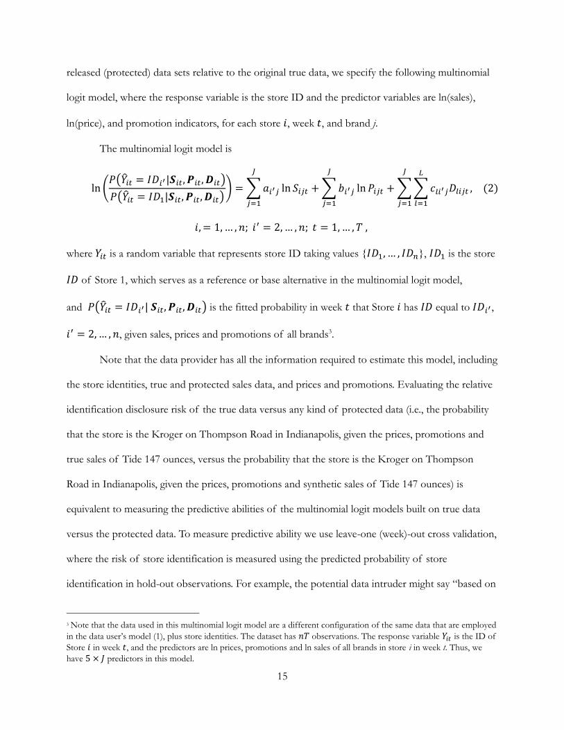
released (protected) data sets relative to the original true data, we specify the following multinomial

logit model, where the response variable is the store ID and the predictor variables are ln(sales),

ln(price), and promotion indicators, for each store 𝑖, week 𝑡, and brand j.

The multinomial logit model is

ln (𝑃(�̂�𝑖𝑡 = 𝐼𝐷𝑖′|𝑺𝑖𝑡, 𝑷𝑖𝑡, 𝑫𝑖𝑡)

𝑃(�̂�𝑖𝑡 = 𝐼𝐷1|𝑺𝑖𝑡, 𝑷𝑖𝑡, 𝑫𝑖𝑡)) = ∑ 𝑎𝑖′𝑗 ln 𝑆𝑖𝑗𝑡

𝐽

𝑗=1

+ ∑ 𝑏𝑖′𝑗 ln 𝑃𝑖𝑗𝑡

𝐽

𝑗=1

+ ∑ ∑ 𝑐𝑙𝑖′𝑗𝐷𝑙𝑖𝑗𝑡

𝐿

𝑙=1

𝐽

𝑗=1

, (2)

𝑖, = 1, … , 𝑛; 𝑖′ = 2, … , 𝑛; 𝑡 = 1, … , 𝑇 ,

where 𝑌𝑖𝑡 is a random variable that represents store ID taking values {𝐼𝐷1, … , 𝐼𝐷𝑛}, 𝐼𝐷1 is the store

𝐼𝐷 of Store 1, which serves as a reference or base alternative in the multinomial logit model,

and 𝑃(�̂�𝑖𝑡 = 𝐼𝐷𝑖′| 𝑺𝑖𝑡, 𝑷𝑖𝑡, 𝑫𝑖𝑡) is the fitted probability in week 𝑡 that Store 𝑖 has 𝐼𝐷 equal to 𝐼𝐷𝑖′ ,

𝑖′ = 2, … , 𝑛, given sales, prices and promotions of all brands3.

Note that the data provider has all the information required to estimate this model, including

the store identities, true and protected sales data, and prices and promotions. Evaluating the relative

identification disclosure risk of the true data versus any kind of protected data (i.e., the probability

that the store is the Kroger on Thompson Road in Indianapolis, given the prices, promotions and

true sales of Tide 147 ounces, versus the probability that the store is the Kroger on Thompson

Road in Indianapolis, given the prices, promotions and synthetic sales of Tide 147 ounces) is

equivalent to measuring the predictive abilities of the multinomial logit models built on true data

versus the protected data. To measure predictive ability we use leave-one (week)-out cross validation,

where the risk of store identification is measured using the predicted probability of store

identification in hold-out observations. For example, the potential data intruder might say “based on

3 Note that the data used in this multinomial logit model are a different configuration of the same data that are employed

in the data user’s model (1), plus store identities. The dataset has 𝑛𝑇 observations. The response variable 𝑌𝑖𝑡 is the ID of

Store 𝑖 in week 𝑡, and the predictors are ln prices, promotions and ln sales of all brands in store i in week t. Thus, we

have 5 × 𝐽 predictors in this model.

16

my available data, I estimate a 25% probability that this observation is from the Kroger on

Thompson Road in Indianapolis.” We present further details in Section 2.4.1 including the kinds of

data that potential intruders may have access to in real life.

2.3 Proposed Data Protection Model

We propose a Bayesian random effects model for protecting data through the use of a

flexible prior distribution that reflects the data provider's risk-return preferences. To begin we

discuss some pertinent questions about the data provider’s process of developing the protected data.

Firstly, the data provider’s goal is to release useful yet privacy-protected data to data users. As

discussed, in our analysis the data provider assesses the identity disclosure risks by measuring the

predictability of store identities based on various forms of protected data compared to the true data.

Secondly, which variables in the data gathered from stores should not be released, and hence

protected by transformation into synthetic data? We use the decision criterion that variables that

have the most power to predict store IDs in the training data should be protected. As discussed later

in our empirical application, we choose to protect sales quantities but not price or promotion data.

We chose these variables based on analysis that is reported in detail in Appendix C, and is described

here conceptually. In our available sample of AC Nielsen data, we use the multinomial logit model

specified in Section 2.2 to compute the ability of variables such as prices, promotions, and sales

volumes, to predict store IDs. Our analysis shows that using prices alone leads to an average loss of

protection of 0.062, while using sales volumes alone leads to a much higher average loss of

protection of 0.511. (See Equation (7) and the related discussion for the definition of Loss of

Protection.) Consequently, we chose to protect sales quantities in our data protection method. Why

do we not protect the prices and promotions as well? There are two reasons over and above their

limited ability to predict store IDs. One, prices and promotions provide valuable information to data

users, such as the distribution of retail prices of own and competing products, and protection would

17

distort this information. Two, unlike brand sales volumes, prices and promotions are publicly

available information that can be observed in the store. Therefore, a determined intruder could

obtain such data with sufficient effort and hence these data are less necessary to protect. While price

and promotion information can also be protected, this would add greater complexity to the models,

and we discuss this idea as a future research opportunity in Section 4.

Third, in developing the protected data, we propose the use of a random effects model

instead of a model-free noise approach (e.g., simply adding a random number to sales). We

implement the model-free noise approach as a benchmark method for comparison. In a random

effects model, the distribution of the dependent variable, i.e. sales quantities, can be altered with

little difficulty to incorporate non-normally distributed data, thus allowing modeling flexibility across

types of data. Additionally, and perhaps most importantly, it is common for estimates of random

effects (e.g. store effects) to rely on only a few observations each. And the privacy-preserving prior

distribution naturally protects the estimates of the random effects from discovery by an intruder by

scaling the estimates of the random effects toward zero, or no information.4

Figure 2 summarizes the process by which the data provider generates protected data to

release to the data user. The protection mechanism we propose shrinks the values of the estimated

random effects and fixed effects toward zero (i.e., the limiting case of no information) through the

use of a privacy-preserving prior distribution on the variances of the random effects and fixed

effects. This is managerially important because the data provider prevents the data intruder from

knowing or approximating the true arithmetic mean of q observations in a small group. Instead, the

protection mechanism scales the estimated values of the q observations toward their greater group

means (e.g., overall intercept of all observations). Our proposed method is nonstandard because it

4 Previous research (Bleninger, Drechsler, and Ronning 2011) has shown that a data intruder can strategically uncover sensitive data (e.g., sales quantities of specific observations) when the data protection method is to simply add noise.

18

first protects the random and fixed effects and then adds noise centered at the protected deviations.

After controlling for all variables and shrinking the estimates of the random and fixed effects toward

zero, we generate the synthetic sales quantities.

Figure 2: Data Provider’s Process for Generating Synthetic Data for Release to the Data User

We describe the base modeling setup and the likelihood in Section 2.3.1. A description of

our flexible protective prior distribution is given in Section 2.3.2. Computational details for

generating synthetic data are provided in Section 2.3.3.

2.3.1 Base Model

We observe a response variable, sales 𝑆𝑖𝑗𝑡 for store 𝑖 = 1, … , 𝑛, brand 𝑗 = 1, … , 𝐽, time 𝑡 =

1, … , 𝑇. Additionally, price, 𝑃𝑖𝑗𝑡 , and promotion indicators 𝐷𝑙𝑖𝑗𝑡 are covariates that affect the

response. Based on Equation (1), for each brand j, we model ln 𝑆𝑖𝑗𝑡 using a random effects model:

ln 𝑆𝑖𝑗𝑡 = 𝜇𝑗 + 𝑢𝑖𝑗 + 𝛽𝑗 ln 𝑃𝑖𝑗𝑡 + ∑(ln 𝛾𝑙𝑗)

𝐿

𝑙=1

𝐷𝑙𝑖𝑗𝑡 + 𝜖𝑖𝑗𝑡 , (3)

where 𝜇𝑗 is the overall intercept of the brand-specific model for brand j, 𝑢𝑖𝑗 is the random (store)

19

effect that is assumed to be normally distributed with zero mean and constant variance 𝜎𝑢2, 𝛽𝑗 and

ln (𝛾𝑙𝑗) are the fixed effects of price and promotions respectively, and 𝜖𝑖𝑗𝑡 is the observation-

specific error term which is normally distributed with constant variance, 𝜏𝑗2.

Note that model (3) is brand-specific, meaning that the model is fitted separately for each

brand 𝑗. For simplicity of notation, we omit the subscript 𝑗 in the rest of Section 2.3 unless

otherwise indicated. A natural way to estimate the random effects model is through Bayesian

modeling with conjugate priors. The Bayesian approach to generate protected (synthetic) data

through a posterior predictive distribution can be traced back to Rubin (1993).

For the prior distribution of all model parameters in (3), the overall intercept term 𝜇 is

assumed to follow a normal distribution with zero mean and a large constant variance 𝐾2 so that the

prior is diffuse. The variance of the random effect, 𝜎𝑢2, is assumed to be distributed according to an

Inverse-Gamma distribution. The fixed effects vector (𝛽, ln 𝜸) is assumed to be jointly distributed

as multivariate normal with a mean vector of zeros and diagonal covariance matrix Σ𝑏. In effect, we

assume each of the fixed effects, (𝛽, ln 𝜸), has the same prior distribution, that is, independent

normal with zero mean and variance 𝜎𝑏25. The variance of model error 𝜏2 is assumed to follow an

Inverse-Gamma distribution with fixed shape and scale parameters.

Formally, we have 𝜇~N(0, 𝐾2); 𝜏2 ~ IG(𝑎0, 𝑏0); 𝜎𝑢2~IG(

𝜈0

2,

𝑉0

2); (𝛽, ln 𝛾)~MVN(0, 𝜎𝑏

2𝐈).

Among the hyper parameters (𝐾2, 𝑎0, 𝑏0, 𝑉0, 𝜈0, 𝜎𝑏2), 𝐾 is set to be a large positive number, 𝑎0 and

𝑏0 are fixed positive numbers, and 𝑉0 and 𝜈0 are functions of a single new protection parameter that

we will elaborate on further in Section 2.3.2. To implement the random effects model (3), we use

5 When the covariance matrix Σ𝑏takes a general form, it is not immediately obvious how to incorporate the protection

parameter even though the full conditionals can still be derived analytically. We leave this extension as a future research opportunity.

20

freely available software, an R package MCMCglmm (Hadfield 2010). Details of the specification of

hyper-parameters are discussed next.

2.3.2 Flexible Prior Distribution

The random effects model can be interpreted as a “mean model” (McCulloch and Searle

2001). Thus, posterior samples of a function of the unprotected parameters, 𝑢𝑖 + 𝛽 ln 𝑃𝑖𝑡 +

∑ (ln 𝛾𝑙)𝐷𝑙𝑖𝑡𝐿𝑙=1 , represent unprotected “deviations” from the intercept of all observations, 𝜇. These

deviations are linear combinations of the data provider’s continuous and categorical variables and

the estimated coefficients (which are conditional on the original unprotected data). Since posterior

samples of the linear predictor 𝑢𝑖 + 𝛽 ln 𝑃𝑖𝑡 + ∑ (ln 𝛾𝑙)𝐷𝑙𝑖𝑡𝐿𝑙=1 can be predictive of the identity of

store i, they require protection.

To achieve data protection, the flexible prior distribution takes information away from the

unprotected deviations by tuning the hyper-parameters of the prior on the variance components. It

scales the unprotected deviations toward no information, as a mechanism for data protection. The

priors on the variable-specific fixed effects and random effects shrink their posterior estimates

toward zero through an adjustable protection parameter. This is motivated by the fact that the

Bayesian estimator with an informative prior is a shrinkage estimator.

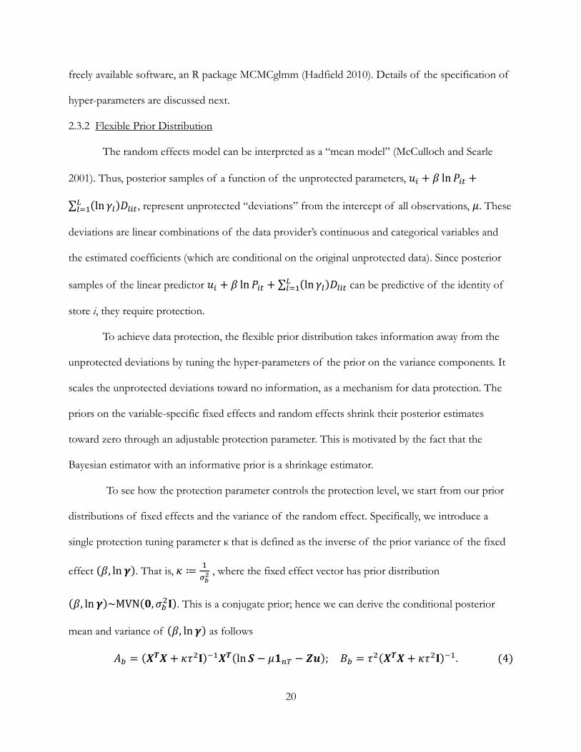
To see how the protection parameter controls the protection level, we start from our prior

distributions of fixed effects and the variance of the random effect. Specifically, we introduce a

single protection tuning parameter к that is defined as the inverse of the prior variance of the fixed

effect (𝛽, ln 𝜸). That is, 𝜅 ≔1

𝜎𝑏2 , where the fixed effect vector has prior distribution

(𝛽, ln 𝜸)~MVN(𝟎, 𝜎𝑏2𝐈). This is a conjugate prior; hence we can derive the conditional posterior

mean and variance of (𝛽, ln 𝜸) as follows

𝐴𝑏 = (𝑿𝑻𝑿 + 𝜅𝜏2𝐈)−1𝑿𝑻(ln 𝑺 − 𝜇𝟏𝑛𝑇 − 𝒁𝒖); 𝐵𝑏 = 𝜏2(𝑿𝑻𝑿 + 𝜅𝜏2𝐈)−1. (4)

21

where, for each brand, using matrix notation, 𝑿 = [ln 𝑷 𝑫1 … 𝑫𝐿], ln 𝑺 is an 𝑛𝑇 dimensional

response vector, 𝑿 is an 𝑛𝑇 × (1 + 𝐿) dimensional covariates matrix for brand 𝑗, 𝒖 is an 𝑛

dimensional random effect vector, and 𝒁 is an 𝑛𝑇 × 𝑛 dimensional indicator matrix for store 𝑖 such

that 𝒁𝒖 = [𝑢1, … , 𝑢1, … , 𝑢𝑖 , … , 𝑢𝑖 , … , 𝑢𝑛, … , 𝑢𝑛] is a 𝑛𝑇 dimensional vector.

We illustrate the role of 𝜅 in generating synthetic data through the posterior form (4). Note

that by using (4) we can shrink the fixed-effect estimates of (𝛽, ln 𝜸) toward 0 by increasing the

parameter 𝜅. At the other extreme, when 𝜅 tends to zero, or equivalently the prior variance 𝜎𝑏2 goes

to infinity, we obtain a diffuse prior, in which case (4) becomes equivalent to the ordinary least

squares estimator.

Hence the single tuning parameter 𝜅 can capture the preference of the data provide with

regard to trading off data protection (privacy) versus information loss. A smaller value of 𝜅

(equivalently, a larger value of hyper-parameter 𝜎𝑏2) results in weaker protection. A larger value of 𝜅

(equivalently, a smaller value of the hyper-parameter 𝜎𝑏2) results in stronger protection. Hence we

term 𝜅 the data privacy protection parameter and each value of 𝜅 corresponds to a particular

implicit tradeoff between information loss and privacy.

The conjugate prior distribution of the variance of the random effect is an inverse-Gamma

distribution 𝜎𝑢2~ IG (

𝜈0

2,

𝑉0

2) with mean

𝑉0

𝜈0−2 and variance

2𝑉02

(𝜈0−2)2(𝜈0−4). The conditional posterior

of 𝜎𝑢2 is �̃�𝑢

2|𝒖 ~ IG (𝑛+𝜈0

2,

𝒖′𝒖+𝑉0

2). To incorporate the privacy protection parameter 𝜅, we set 𝑉0 =

1

10𝜅 and 𝜈0 = 100𝜅, which makes the mean arbitrarily close to zero as 𝜅 increases. With this

specification of hyper-parameters, a larger value of 𝜅 is equivalent to stronger informative priors for

both (𝛽, ln 𝜸) and 𝜎𝑢2. Since the means of (𝛽, ln 𝜸) and 𝜎𝑢

2 are 0 and 𝑉0

𝜈0−2, respectively, a stronger

informative prior shrinks the posteriors toward their respective means.

22

Note that one can specify different forms of 𝑉0 and 𝜈0 to incorporate 𝜅. Generally, a

stronger protection corresponds to a smaller value of 𝑉0 and a larger value of 𝜈0 such that both the

mean and variance of �̃�𝑢2 tend to 0, and equivalently the posterior samples of the random effect, 𝑢𝑖 ,

scale toward zero. The full conditionals for the other model parameters can be easily derived

analytically. We present details in Appendix B.

2.3.3Protected Data for Release to Data User

The proposed data protection method generates protected synthetic values of ln 𝑆𝑖𝑡 for valid

use by data users. These synthetic values, ln �̃�𝑖𝑡, are generated by sampling from the protected

posterior predictive distribution, which contains the protected model parameters, (𝛽, ln �̃�) and �̃�.

To do this, we first run the MCMC with a set number of iterations as a burn-in. Then, for the

remaining iterations, 𝑚 = 1, … , 𝑀, all posterior samples of the protected model parameters are

saved. After verifying convergence of the posterior samples of all parameters, for each iteration 𝑚

and each observation 𝑖𝑡, the protected deviation, �̃�𝑖 + 𝛽 ̃ ln 𝑃𝑖𝑡 + ∑ (ln �̃�𝑙)𝐿𝑙=1 𝐷𝑙𝑖𝑡, is

calculated. Then, a disturbance term 𝜖𝑖𝑡 is sampled from a normal distribution with mean zero and

variance �̃�2, the posterior sample of residual variance. The sum of the protected deviation and the

disturbance results in a single protected synthetic value. Together, for each brand j, the protected

deviation, disturbance, and associated intercepts and covariates determine the protected posterior

predictive distribution for each observation 𝑖𝑡,

𝐹𝑖𝑡𝑝(𝜅) = 𝑝(ln �̃�𝑖𝑡 |𝑺, 𝑷, 𝑫, 𝜅, 𝑎0, 𝑏0, 𝐾) = ∫ 𝑝(ln �̃�𝑖𝑡 |𝜣; ln 𝑃𝑖𝑡 , 𝑫𝑖𝑡) × 𝑝(𝜣|𝜣𝐻, 𝑺, 𝑷, 𝑫)𝑑𝜣

𝜣

, (5)

where 𝜣 = (𝜇, 𝛽, ln 𝜸 , 𝒖, 𝜎𝑢 2 , 𝜏

2) is the vector of model parameters, and 𝜣𝑯 is the vector of hyper

parameters for priors.

This process can be repeated for a desired number of protected synthetic vectors for all

23

brands, ln �̃�, of length 𝑛 × 𝐽 × 𝑇. We suggest that the data provider releases only one vector of

synthetic data to the data user so that it can reduce the chance of protected model parameters being

subject to invalid use. For a detailed discussion see Reiter, Wang, and Zhang (2014) who found that

multiple releases of synthetic data are more informative of the confidential data. In this regard note

that multiple releases of synthetic data for the same time period are similar to releasing all the

parameters of a model and disclosing the entire posterior distribution.

2.4 Criteria to Measure Performance of Data Protection Method

As noted, all data protection methods imply a tradeoff between two criteria: identity

disclosure risk and information loss. This tradeoff can be analyzed using a Risk-Utility curve

(Duncan et al. 2001) which represents the natural tradeoff between data protection and the utility of

valid use. We discuss these two criteria in detail next.

2.4.1 Measures of Identification Disclosure Risk

In order to evaluate the identification disclosure risk of the protected data versus the true

data, we adopt a leave-one (week)-out cross validation approach. Figure 3 gives a flow chart that

describes the steps to compute measures of identification disclosure risk for various released data

sets as well as for releasing the true data.

24

Figure 3: Leave-One (Week)-Out Cross Validation Process for True Data and Various Released (Protected) Data

Specifically, for each week 𝑘, 𝑘 = 1, … , 𝑇, a multinomial logit model (2) is estimated using

(T-1) weeks of available data 𝑨 = {𝑌𝑖𝑡, �̃�𝒊𝒕, 𝑷𝒊𝒕, 𝑫𝒊𝒕}, 𝑖 = 1, … , 𝑛 stores and 𝑡 = 1, … (−𝑘), … , 𝑇

weeks. 𝑌𝑖𝑡 is the true store ID of Store i in week t, �̃�𝒊𝒕 represents the J-vector of protected sales

(using the proposed method or any benchmark method), 𝑷𝒊𝒕 is the J-vector of prices, and 𝑫𝒊𝒕 is the

Start

Leave out kth week observations, k = 1, …, T, and build a

Multinomial Logit Model using the remaining (T-1) weeks of

data

Data provider has all observations with sales (true

or protected), prices, promotions and store IDs

Predict Store ID probability for each store i, i = 1, ….,n for held-out week k. Retain these predicted probabilities

Update week k = k+1

Is k = T?

No

Yes

Compute mean Store ID probabilities for each store, across weeks. Use these values

to compute 𝐿𝑃𝑖 , i = 1,…,n

Obtain summary measures from distribution

of 𝐿𝑃𝑖 : MLP and ALP

25

(L*J) vector of promotions. Here (−𝑘) indicates that information for week 𝑘 is not used for

estimating the multinomial logit model (2). The probabilities 𝑃(�̂�𝑖𝑘 = 𝐼𝐷𝑖′) of the left-out kth-week

store ID are then calculated for the fitted model (2) using the following explanatory variables

{�̃�𝒊𝒌, 𝑷𝒊𝒌, 𝑫𝒊𝒌}, 𝑖 = 1, … , 𝑛 . For the special case in which the identity disclosure risk of true data is

evaluated, the true sales 𝑺𝒊𝒕 are used.

Note that in our particular empirical application (discussed in Section 3), for each held-out

week we obtain an 𝑛 × 𝑛 predicted conditional probability matrix, which is calculated by plugging in

values of covariates (sales, prices, and promotions) into the estimated multinomial logit model

(2). In this case, the predictive model has the limitation that it does not incorporate the information

that the hold-out sample contains exactly n distinct masked entities, and there are n distinct entities

in the training sample. In other words, the column sum of the probability matrix, i.e., ∑ 𝑃𝑛𝑖 (�̂�𝑖𝑘 =

𝐼𝐷𝑖′), is not guaranteed to be 1. In practice, however, in the data multiple records for a brand in a

given period could be from the same store depending on, for instance, how SKUs are aggregated.

Not imposing the constraint implies that there are measurement errors associated with sales so that

multiple samples of the same store for the same period may result in different sales measures. We

would like to emphasize that frequently in practice, the number of stores whose identity is to be

predicted is very likely to be smaller than the number of stores used in the training sample.

Therefore, the constraint should not be imposed in general. Despite this limitation of the predictive

model in our application, it appears to be a natural first attempt in identifying store identities.

For each Store 𝑖, the predicted probability that its store ID is 𝑖′ is computed as the mean of

the predicted probability vector across held-out weeks to obtain the n-vector {𝑃(�̂�𝑖 =

26

𝐼𝐷1), … , 𝑃(�̂�𝑖 = 𝐼𝐷𝑛)} :

𝑃 (�̂�𝑖 = 𝐼𝐷𝑖′

) =1

𝑇∑ 𝑃 (�̂�𝑖𝑘 = 𝐼𝐷

𝑖′)

𝑇

𝑘=1

, (6)

where 𝑃(�̂�𝑖𝑘 = 𝐼𝐷𝑖′) is the predicted probability that Store 𝑖 is Store 𝑖′, 𝑖′ = 2, … , 𝑛, in the held-out

week k.

The proposed method uses a (pseudo) out-of-sample fit criterion to avoid overfitting and to

mimic the prediction problem for the potential intruder: synthetic sales and covariates are known,

and the objective is to predict store identities. One way to do this is to use data for 𝑇 − 1 weeks and

predict the data for the omitted week. To avoid capitalizing on the idiosyncrasies of just one week,

the method repeatedly leaves out one week at a time (𝑘 = 1, … , 𝑇) and uses 𝑇 − 1 observations to

predict store IDs for week 𝑘. An alternative way is to split the data into an estimation sample (weeks

1,2, … , 𝑇′) and a validation sample (weeks 𝑇′ + 1, … , 𝑇). Both holdout methods are used in the

robustness check in Section 3.5.

We define the following measure, called Loss of Protection (𝐿𝑃𝑖), for Store 𝑖:

𝐿𝑃𝑖 = √𝑛 ∑[𝑃(�̂�𝑖 = 𝐼𝐷𝑖′)]2

𝑛

𝑖′=1

− 1. (7)

In summary, 𝐿𝑃𝑖 measures the intruder’s confidence in the ability of the available data to identify

Store 𝑖. 𝐿𝑃𝑖 also has a natural lower bound of 0 for randomly guessing the identity of store 𝑖 where

𝑃(�̂�𝑖 = 𝐼𝐷1) = 𝑃(�̂�𝑖 = 𝐼𝐷2) = ⋯ = 𝑃(�̂�𝑖 = 𝐼𝐷𝑛) = 1/𝑛. It has an upper bound of √𝑛 − 1 if

one store identification probability is 100% and each of the other probabilities is 0%. In general, a

smaller value of 𝐿𝑃𝑖 implies that the individual store is better protected. 𝐿𝑃𝑖 thus captures the

variability of store identification probabilities (or intruder confidence).

27

Note that for market-level data, 𝐿𝑃𝑖 cannot be computed because there is no store

information at all in the data. Therefore, we define the 𝐿𝑃𝑖 of market-level data as 0. Our proposed

𝐿𝑃𝑖 measure is closely related to, but distinct from, popular measures in the literature on information

theory, such as Gini impurity, which is commonly used in classification trees (Breiman et al., 1984),

and Entropy.6 The use of Gini impurity and Entropy in classification trees, however, is very different

from using the proposed 𝐿𝑃𝑖 measure, although there is strong similarity in the formulae. Gini

impurity and Entropy are mainly used to measure the impurity of a node in decision trees; however,

the proposed 𝐿𝑃𝑖 statistic is a measure of loss of protection based on estimated probabilities of

store identification.

As a measure of the protection level for the full set of stores, we propose using Maximum

Loss of Protection (MLP), which is calculated as:

𝑀𝐿𝑃 = max{𝐿𝑃1, … , 𝐿𝑃𝑛}. (8)

MLP is useful in measuring the minimum level of privacy across all stores; this measure is especially

useful to a data provider concerned with the problems arising from the identification of any store.

In addition to MLP, one can use other statistics such as average, median, and minimum 𝐿𝑃𝑖 . For

example, Average Loss of Protection (ALP) can be used as an overall measure of the protection

level for the full set of stores.

The leave-one (week)-out cross validation approach we use helps the data provider to

evaluate the out-of-sample predictability of store IDs based on the released protected data versus

the true data. An alternative view of this process is that the data user or intruder has access to

6 In our particular case, Gini impurity for store 𝑖 can be written as Gini𝑖 = 1 − ∑ 𝑃(�̂�𝑖 = 𝐼𝐷𝑖′)2𝑛

𝑖′ . It is easy to see the

link between LP and Gini impurity. 𝐿𝑃𝑖 = √𝑛 ∑ 𝑃(�̂�𝑖 = 𝐼𝐷𝑖′)2𝑛

𝑖′=1 − 1 = √𝑛(1 − 𝐺𝑖𝑛𝑖𝑖) − 1. Entropy for Store i is

defined as Entropy𝑖 = − ∑ [𝑃(�̂�𝑖 = ID𝑖′)] log2 𝑃(�̂�𝑖 = ID𝑖′)𝑛𝑖′=1 .

28

training data with protected or true sales, and the true store IDs. The data user or intruder can then

use these data as a training sample to build a predictive multinomial logit model of store IDs. In the

AC Nielsen context, potential sources of such training data are individual retailers, and retail chains

or wholesalers who directly sell or share their own data, and/or allow store identities to be

observed.7 This model can then be used to predict store identities in newly released data in which

store IDs have been disguised (in Appendix E we show a simple example of this prediction

process).

To make this idea more precise, say the data user or intruder has access to historical released

data (with protected or true sales) with true store identities (e.g., “these are the prices and the

(synthetic) sales of Tide 147 at the Kroger on Thompson Road in Indianapolis”): 𝑨 =

{𝑌𝑖𝑡, �̃�𝒊𝒕(𝒐𝒓 𝑺𝒊𝒕), 𝑷𝒊𝒕, 𝑫𝒊𝒕}, 𝑡 = 1,2, … , 𝑇′. The data user or intruder builds a predictive multinomial

logit model on 𝑨 and uses the estimates to predict the store identities, �̂�𝑖(𝑡=𝑇′+1,…,𝑇) in newly

released data 𝑅 = {�̃�𝒊𝒕, 𝑷𝒊𝒕, 𝑫𝒊𝒕}, 𝑡 = 𝑇′ + 1, … , 𝑇. Note that the subscript 𝑖 indicates that the data

user receives a hashed version of store IDs in the newly released data so that it does not know the

store identities, but knows which weekly observations belong to the same store. We provide

empirical results based on this type of analysis in Section 3.5. Importantly, the results from using

this method are qualitatively consistent with those from the leave-one (week) out cross validation

approach.

2.4.2 Measures of Information Loss Due to Data Protection

In our discussion of information loss from data protection, our empirical analysis focuses

7 Some examples of retailers’ data sharing programs include Retail Link (Walmart), Partners Online (Target), Workbench

(Sears) and Vendor Dart (Lowe’s). The primary goals of such programs are to facilitate better management of shipments, inventory, out-of-stocks and forecasts, often at the store level. Note that these data are typically not a substitute for retail data provided by syndicated data providers like AC Nielsen, which are based on careful sampling of stores and hence provide the benefits of being able to project sales volumes, market shares, prices, and promotional activities to regional and national markets.

29

mainly on the estimated own-price elasticities; similar ideas apply to the estimated promotion

effects. Since price elasticities are a key metric in determining optimal mark-ups and profitability, and

for conducting “what if ” analyses, we assume that an important goal of data users is to correctly

estimate these own price elasticities. The estimates from the “unprotected” (true) store-level data are

taken to be the true elasticities 𝛽𝑗 . Information loss under any data protection method is measured

as the Mean Absolute Percentage Deviation (MAPD) of the estimated price elasticities based on the

protected data, �̂�𝑗 , from the true 𝛽𝑗 :

𝑀𝐴𝑃𝐷 =1

𝐽∑ |

�̂�𝑗 − 𝛽𝑗

𝛽𝑗|

𝐽

𝑗=1

× 100%. (9)

Additionally, MSE is defined as the Mean Squared Error of parameter estimates from using

protected data compared to the corresponding parameter estimates from using the original data.

𝑀𝑆𝐸 =1

𝐽∑(�̂�𝑗 − 𝛽𝑗)

2

𝐽

𝑗=1

.

In our paper, we disregard estimation uncertainty; consequently, we assume that the

original, unprotected store-level data has a MAPD and MSE of 0%. Since an important managerial

use of estimated elasticities is determining optimal prices (e.g., Reibstein and Gatignon 1984), we

also compute for each brand the optimal mark-up over marginal cost (MC), defined as

𝑂𝑝𝑡𝑖𝑚𝑎𝑙 𝑀𝑈𝑗% =𝑃𝑟𝑖𝑐𝑒𝑗 − 𝑀𝐶𝑗

𝑀𝐶𝑗× 100% =

1

|𝛽𝑗| − 1× 100%. (10)

Additionally, we compute the deviations from optimal profits (i.e., maximum profit using the true

data) as another measure of the loss of information. For the SCAN*PRO model, which is a

constant elasticity sales response model, the assumption of constant marginal cost for any brand

yields the following expression for the ratio of optimal profits relative to the no protection case ( the

j subscript has been suppressed throughout in the expression for simplification; the derivation of

30

this formula is shown in Appendix D):

Π̂

Π=

Π(�̂�)

Π(𝑃)= (

�̂� − 𝐶

𝑃 − 𝐶) (

�̂�

𝑃)

𝛽

= (𝛽 + 1

�̂� + 1) (

𝛽 + 1

�̂� + 1

�̂�

𝛽 )

𝛽

, (11)

where Π̂ and �̂� are the optimal profit and optimal price, respectively, based on the estimated price

elasticities from protected data, whereas Π and 𝑃 are the optimal profit and optimal price,

respectively, based on the price elasticities estimated using unprotected data.

Note that estimates of elasticities that are of absolute magnitude smaller than 1 result in

meaningless estimates of both the optimal markup and the deviation from optimal profits. We point

out these cases in our discussion of empirical results as indications of the lack of face validity of the

estimated elasticities.

3. Empirical Application

We apply the model in (1) to AC Nielsen point-of-sale scanner data for five brand-sizes of

powdered detergents from the three largest brands in the market: 72 and 147-ounce packs of Tide

and Oxydol and the 72-ounce pack of Cheer. The data are weekly store-level sales, prices and

promotions in 34 stores in Sioux Falls, SD, and Springfield, MO, collected over 102 weeks. These

data have also been used in Christen et al. (1997).

To compute measures of loss of protection, we conduct analysis similar to leave-one-out

cross validation as discussed in Section 2.4.1. We use all-but-one week of observations of data (𝑨 =

{𝑌𝑖𝑡, �̃�𝒊𝒕, 𝑷𝒊𝒕, 𝑫𝒊𝒕}, 𝑖 = 1, … , 𝑛 stores and 𝑡 = 1, … (−𝑘), … , 𝑇 weeks) to predict the store ID for

the left-one-out observation. We repeat this process for all weeks and compute all reported measures

of loss of protection.

We compare the performance of the proposed method with the performances of seven

benchmark data protection methods. Benchmark Method 1 is the unprotected, store-level data, where

31

we have no information loss by definition, and the largest loss of protection. Benchmark Methods 2,

3, 4, 5, and 6, respectively, are as follows: adding random noise, rounding, top coding, 20% swapping,

and 50% swapping. Finally, Benchmark Method 7 is based on using (aggregated) market-level data,

which reflects the type of data AC Nielsen offers its clients. See the definitions in Table 1.

For adding random noise, due to the large variance of original sales, we first bin observations

into deciles based on sales, and then add random noise for each bin separately using its empirical

variance. For rounding, the unprotected sales are simply rounded to the nearest hundred. For top

coding, any observation in which sales is greater than the 95th percentile is truncated so that extreme

values can be protected. For swapping, we chose a specified percentage of observations (20% and

50% in our analysis) at random and divided these observations into two groups at random. Then the

values of sales were exchanged between these two groups. The remaining variables, namely store ID,

prices, displays, and feature were unchanged.

Table 1: Definition of Benchmark Protection Methods

Benchmark Method Description

1 “True” or Unprotected Store-Level Data

Original store-level sales data without any protection

2 Random Noise Observations are binned into deciles based on sales, and random noise is added to the sales in each decile

3 Rounding Sales are rounded to the nearest hundred

4 Top Coding Sales greater than the 95th percentile are truncated

5 20% Swapping 20% of observations are divided into two groups and their sales data are exchanged

6 50% Swapping 50% of observations are divided into two groups and their sales data are exchanged

7 Market-Level For each week sales are summed and prices and promotions are averaged across stores to the market level

3.1 Trade-Off Between Information Loss and Loss of Protection

We focus first on the loss of information with respect to estimates of the own-price

elasticities of the five brand-sizes as measured by MAPD, and loss of protection as measured by our

proposed measure, MLP. The reason to focus on MLP (instead of ALP) is that this measure

32

corresponds to a worst-case scenario and reflects the largest potential cost to the data provider from

disclosure of even one store’s ID. Figure 4 shows the results of our proposed method as we vary к

from 0.1 to 15, as well as those for the seven benchmark methods8.

As discussed, in the proposed method, is a managerially determined parameter that

reflects the trade-off between the level of protection and information loss. As expected, increasing

leads to greater information loss, and reduces the ability of the data user to accurately estimate

price elasticities. In addition, it protects the data by lowering the risk of identification of store IDs.

The choice of reflects the criterion selected by the data provider to choose the preferred tradeoff

between the level of protection across all stores and the implicit degree of precision in estimating

elasticities that the data provider chooses to offer its clients.

Figure 4. Performance of Alternative Data Protection Methods

8 We are grateful to an anonymous reviewer for useful suggestions on the presentation of Figure 4 and its interpretation.

33

Figure 4 shows that there are considerable differences in the performances of the different methods

using the two criteria: information loss and loss of protection. Importantly, Figure 4 makes it clear

that the choice of a data protection strategy requires the firm to make a tradeoff between these

criteria. We note that while AC Nielsen’s extant approach of aggregating data to the market-level is

the most effective in terms of protection, it leads to substantial loss of information with an MAPD

of 43.7%. This result is consistent with the literature on aggregation bias (Christen et al. 1997)

which reports large biases in parameter estimates due to aggregation.

Note that none of the benchmark methods dominates (i.e. lies to the southwest of) the

proposed method at any level of к. By using the proposed method, the data provider has the choice

of giving up protection in order to provide more information. For instance, a data provider who

faces strong competition from rival data providers who promise clients higher data quality may

decide to pursue that option by choosing smaller values of к.

34

We see from Figure 4 that random noise, top coding, and rounding, offer the same levels of

protection as the original store-level data, but lead to greater loss of information. Thus, given our

data it would not be prudent for the data provider to use these methods. Although 50% swapping

and 20% swapping provide greater protection than store-level data, they imply considerable loss of

information. Nevertheless, both methods dominate providing market-level data and hence are

reasonable options for the data provider to consider. Our proposed method allows the decision

maker the flexibility through the choice of к to choose a data protection strategy that dominates

both 20% swapping and 50% swapping. For illustrative purposes, the results shown henceforth for

the proposed method assume к = 1.

As an illustration we show in Figure 5 the average predicted probabilities from the estimated

multinomial logit model where the observed prices, promotions and sales come from each of the 34

stores. The probabilities are shown for both the true sales data and synthetic sales data (generated

using the proposed method with κ=1) and are based on Equation (6). Note that the data in fact

come from Store 12. The figure shows that the true data give the intruder relatively high confidence

(average predicted probability is about 25% and the largest among the 34 probabilities) that the

released data are from Store 12. By contrast, the synthetic data give the intruder much lower

confidence (average predicted probability is about 5%) that the released data are from Store 12.

Note that 5% is close to the outcome from random guessing, which has a corresponding

identification probability of 1/34 (2.9%). From a managerial perspective, this drastic change in

intruder confidence about the discoverability of store ID (25% to 5%) could imply the difference

between the intruder taking an undesirable action (from the data provider’s perspective) or not.

Figure 5. Average Predicted Probabilities that Observed Point-of-Sale Data from Store 12 Came From Each of the 34 Stores

35

3.2 Price Elasticities and Implied Optimal Markups and Profits

Table 2 reports the profit-maximizing percentage markups over marginal cost based on the

estimated price elasticities from the proposed and benchmark methods, for each of the five brand-

sizes. If the estimated price elasticity is smaller than one in absolute value, the optimal mark-up is

“not meaningful”, and we indicate this as NM in the table. Taking the optimal mark-ups in the

“Unprotected (True)” row to be the true mark-ups, we find that the extent of deviation from the

true mark-ups for the other methods roughly corresponds with the loss of information indicated by

the MAPD in Figure 4. However, we see some systematic deviations.

Rounding and random noise lead to small deviations as expected based on their close-to-

zero MAPDs. We find that Top Coding, 20% Swapping, 50% Swapping and Market-level data each

have at least one instance of “not meaningful” mark-ups, with 50% Swapping leading to NM results

for all five brand-sizes. Such results would lead data users to question the validity of the protection

method. Furthermore, Top Coding and 20% Swapping lead to larger-than-true optimal mark-ups in

36

all cases when the results are meaningful. By contrast, market-level data lead to smaller-than-true

optimal mark-ups for the four brand-sizes for which results are meaningful. This is consistent with

past literature (e.g. Christen et al. 1997) which shows that market-level data often overestimate the

magnitude of the own price elasticity.

The mark-up results for the proposed method are reasonable ranging from the worst case

of Tide 147 where the estimated mark-up is 65% of the true value in the first row of Table 2, to the

best case of Oxydol 147 with a mark-up of 108% of the true value. For all brands the estimated

mark-ups are closer to the true markups than those implied by market-level data.

Table 2: Optimal Mark-Up Percentages Implied by Estimated Price Elasticities

Tide 72 Tide 147 Cheer 147 Oxydol 72 Oxydol 147

Unprotected (True) 144.0 267.9 168.9 186.7 214.8

Random Noise 128.3 121.3 176.7 153.1 225.5

Rounding 137.5 237.9 133.9 186.5 172.6

Top Coding 183.9 NM 193.8 213.0 234.5

20% Swapping 405.3 NM 272.0 478.4 491.4

50% Swapping NM NM NM NM NM

Market-Level 115.1 77.9 74.8 NM 153.8

Proposed Method (κ=1) 120.3 175.5 113.9 117.6 232.0

NM: Not Meaningful

Table 3 shows the ratios of optimal profits computed under each data protection method

relative to optimal profits under the unprotected scenario. Consistent with the results on optimal

mark-ups, we see that rounding and random noise lead to close to optimal profits for all five brand-

sizes. In cases where the optimal mark-up shown in Table 2 is not meaningful NM), the ratios of

optimal profits cannot be computed and are shown as not available (NA) in Table 3. Disregarding

those cases, the ratios under top coding are close to 100% with the exception of one brand (Tide

147) where the ratio is about 51%. Under 20% swapping we find poor results for four of five

brands, and under market-level data we find poor results for three of five brands.

Under the proposed method we find good results for four of five brands, and the worst

37

case brand is Cheer 147 with a ratio of about 96%. Note that in the current empirical application (a

constant elasticity demand function with constant marginal costs), the profit function for many of

the brands appears to be quite flat near the maximum, suggesting that the cost to the user of

imprecision in elasticities is relatively small. This finding may not hold in more complex models.

Table 3: Ratio of Optimal Profits Relative to Unprotected Case

Tide 72 Tide 147 Cheer 147 Oxydol 72 Oxydol 147

Unprotected (True) 100.00% 100.00% 100.00% 100.00% 100.00%

Random Noise 99.94% 99.13% 99.19% 99.44% 99.98%

Rounding 99.96% 99.80% 98.99% 100.00% 99.23%

Top Coding 98.80% 50.87% 99.65% 99.70% 99.88%

20% Swapping 81.98% NA 96.08% 87.19% 90.78%

50% Swapping NA NA NA NA NA

Market-Level 98.97% 78.87% 87.91% NA 98.17%

Proposed Method (κ=1) 99.59% 98.90% 95.88% 99.87% 99.51%

NA: Not Available

3.3 Comparison with Market-Level Data

In Table 4 we turn our attention to a comparison of the estimated price and promotion

effects for AC Nielsen’s extant method of data protection – market-level data – with the

corresponding estimates for the proposed data protection method.

Table 4: Estimates of Price and Promotion Effects: Comparison of Results from Market-Level Data and Proposed Method

Coefficient Estimates Relative Differencea

Store-Level

Market-Level

Proposed

( =1)

Market-Level

Proposed

( =1)

Price

Tide 72 -1.69 -1.87 -1.80 10.3% 6.5%

Tide 147 -1.37 -2.28 -1.42 66.3% 3.9%

Cheer 147 -1.59 -2.34 -1.95 46.8% 22.4%

Oxydol 72 -1.54 -0.27 -1.59 -82.4% 3.5%

Oxydol 147 -1.47 -1.65 -1.55 12.6% 5.7%

Absolute averageb 43.7% 8.4%

Feature Only

Tide 72 2.56 5.68 2.63 121.9% 2.8%

Tide 147 2.41 3.52 2.11 46.0% -12.4%

Cheer 147 10.75 9.40 9.69 -12.6% -9.9%

Oxydol 72 4.91 34.78 5.49 609.1% 11.7%

Oxydol 147 4.47 36.33 4.04 712.7% -9.7%

38

Absolute averageb 300.5% 9.3%

Display Only

Tide 72 2.61 20.59 2.88 688.9% 10.5%

Tide 147 2.44 13.09 2.21 436.5% -9.2%

Cheer 147 5.83 14.34 5.68 146.0% -2.6%

Oxydol 72 3.48 23.08 3.38 562.9% -2.8%

Oxydol 147 5.00 121.25 5.65 2325.4% 13.1%

Absolute averageb 831.9% 7.6%

Feature and Display

Tide 72 4.51 0.97 3.93 -78.4% -12.9%

Tide 147 5.74 3.22 6.58 -44.0% 14.7%

Cheer 147 14.94 3.29E+13 9.57 -36.0%

Oxydol 72 6.10 0.18 5.29 -97.0% -13.3%

Oxydol 147 6.16 0.00 7.63 -99.9% 23.9%

Absolute averageb 79.9%c 16.2% c

Adjusted 𝑅2(avg.) 0.958 0.522 0.957 aRelative difference = (Estimate – Store-level estimate)/Store-level estimate. bAbsoluteaverage is defined as the average of absolute value of relative difference. cAbsolute averages for Feature and Display do not include brand-size Cheer 147 because of the unreasonably large estimated effect for market-level data.

We find that the absolute averages of the relative differences for each of price, display only,

feature only, and display and feature effects are substantially, and in some cases dramatically, smaller

for the proposed method than the corresponding effects computed using market-level data. For the

promotion effects in particular, some of the deviations of market-level estimates are unreasonably

large, similar to the results of Christen et al. (1997). See, for instance, the estimates of the effects of

display only and feature only for the two sizes of Oxydol, and the estimate of feature and display for

Cheer 147. These results suggest that our proposed method can relatively easily dominate the extant

approach of aggregating data to the market level in terms of information if the data provider is

willing to tolerate a somewhat higher level of risk of disclosure of store identities.

3.4 Impact of Kappa

In Figure 6 we show the values of model parameters as the data protection parameter κ

changes. We find that all parameters tend toward zero as κ increases, further demonstrating the

tradeoff between data protection and information.

39

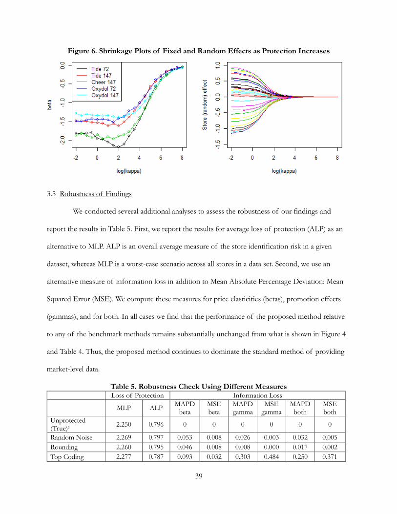
Figure 6. Shrinkage Plots of Fixed and Random Effects as Protection Increases

3.5 Robustness of Findings

We conducted several additional analyses to assess the robustness of our findings and

report the results in Table 5. First, we report the results for average loss of protection (ALP) as an

alternative to MLP. ALP is an overall average measure of the store identification risk in a given

dataset, whereas MLP is a worst-case scenario across all stores in a data set. Second, we use an

alternative measure of information loss in addition to Mean Absolute Percentage Deviation: Mean

Squared Error (MSE). We compute these measures for price elasticities (betas), promotion effects

(gammas), and for both. In all cases we find that the performance of the proposed method relative

to any of the benchmark methods remains substantially unchanged from what is shown in Figure 4

and Table 4. Thus, the proposed method continues to dominate the standard method of providing

market-level data.

Table 5. Robustness Check Using Different Measures Loss of Protection Information Loss

MLP ALP MAPD

beta MSE beta

MAPD gamma

MSE gamma

MAPD both

MSE both

Unprotected (True)1

2.250 0.796 0 0 0 0 0 0

Random Noise 2.269 0.797 0.053 0.008 0.026 0.003 0.032 0.005

Rounding 2.260 0.795 0.046 0.008 0.008 0.000 0.017 0.002

Top Coding 2.277 0.787 0.093 0.032 0.303 0.484 0.250 0.371

40

20% Swapping 1.471 0.425 0.243 0.141 0.266 0.261 0.260 0.231

50% Swapping 1.025 0.180 0.445 0.498 0.437 0.487 0.439 0.490

Market-Level2 0 0 0.437 0.610 1.995 60.630 1.606 45.625

Proposed Method

( =1) 1.566 0.478 0.084 0.026 0.115 0.130 0.108 0.104

Notes: 1. For Unprotected, the metrics for information loss are 0 by definition. 2. For market-level data, we assume that the predicted probabilities for each store ID are equal; that is, 1/n for n=34 stores. Therefore, by the definition of the loss of protection metrics, we have MLP=ALP=0.

As a robustness check we also considered a situation in which the data user or intruder has

access to some historical true sales data with true store identities, as discussed in Section 2.4.1 where

the available training data 𝑨 = {𝑌𝑖𝑡, 𝑺𝒊𝒕, 𝑷𝒊𝒕, 𝑫𝒊𝒕}, 𝑡 = 1,2, … , 𝑇′ is used to predict the store

identities, �̂�𝑖(𝑡=𝑇′+1,…,𝑇) using newly released data 𝑅 = {�̃�𝒊𝒕, 𝑷𝒊𝒕, 𝑫𝒊𝒕}, 𝑡 = 𝑇′ + 1, … , 𝑇. Table 6

gives the ALP and MLP estimates based on the proposed method and benchmark methods when

half of true sales data from week 1 till week 𝑇′ = 51 are used to estimate a multinomial logit model

for store-ID prediction, and predictions of store IDs are made in the remaining weeks 52 to 𝑇 =

102. In addition, we conducted analyses when different proportions of data or protected data 𝑨 =

{𝑌𝑖𝑡, �̃�𝒊𝒕 (𝑜𝑟 𝑺𝒊𝒕), 𝑷𝒊𝒕, 𝑫𝒊𝒕} are used to build the multinomial logit model. Overall, the results are

qualitatively consistent with those from the leave-one (week) out cross validation.

Table 6. Robustness Analysis for the Scenario When the Intruder Has True Historical Sales Data and True Store IDs

Protection Method ALP MLP

Unprotected (True) 0.773 1.649 Random Noise 0.754 1.641 Rounding 0.776 1.628 Top Coding 0.766 1.649 20% Swapping 0.556 1.058 50% Swapping 0.412 0.994 Proposed 0.419 1.143

4. Conclusions and Future Research Directions

This paper proposes a synthetic data methodology that captures the roles of three parties:

the data provider as a commercial supplier who protects data with a data protection method, the

41

data user as a customer, and the potential data intruder. A key distinguishing feature of our

framework relative to the privacy literature in statistics and computer science is that we explicitly

recognize the business goals of the data user as reflected in the data user’s model, and incorporate

these into the data provider’s model for protecting data. We propose a flexible Bayesian

methodology in which the decision maker uses a tuning parameter (к) to analyze the tradeoff

between the conflicting goals of profitability and risk of data disclosure (confidentiality). We

measure information loss using the Mean Absolute Percentage Deviation (MAPD) criterion. In

addition, we propose two new metrics to measure the risk of data disclosure: Average Loss of

Protection (ALP) and Maximum Loss of Protection (MLP).

We test the proposed methodology using retail point-of-sale data marketed by a vendor to its

commercial customers. The vendor sells data but seeks to protect the identities of sample stores

from potential intruders (confidentiality). By contrast, commercial customers use the data to

estimate brand-level price elasticities to determine optimal mark-ups, and the sales effects of

promotions. We show that by enabling the data provider to choose the degree of protection to

infuse into the synthetic data, our method performs well relative to seven benchmark data protection

methods, including the extant approach of aggregating data across stores (e.g., AC Nielsen).

An important limitation of the proposed identification disclosure risk model in the

empirical application reported in this paper is that the estimated probabilities of an observation

belonging to stores in a given time period do not sum to 100%. Development of estimation

approaches that can incorporate this constraint when needed is an important area for future

research. Further, it is important to recognize that our framework and approach are most relevant

when it is possible for a data provider to identify a primary valid use model of data users. In our

application, we used the SCAN*PRO model which is widely employed by users of AC Nielsen retail

data. In such situations our proposed method allows the data provider to protect the data taking

42

account of its data users’ business goals. In other situations where the data user's primary purpose is

to use the data to conduct exploratory analysis, implying that data users’ models are not well

structured, or different data users have very different models, our framework is not as directly

applicable. An example of exploratory analysis is examining the distribution of sales volumes across

stores for the purpose of creating retail segments. Although our framework was not specifically

geared toward such analysis, we found (results are not shown in this paper for reasons of space) that

using synthetic store-level data produced similar results to using the true store-level data. Note that

such retail segmentation analysis cannot be performed using the market-level data currently released

by vendors such as AC Nielsen. Additionally, a data user may be interested in knowing the precision

of the synthetic data relative to the true data. When the measures of precision are for market-level

statistics such as brand sales or brand market shares, we don’t expect such additional information to

change the level of protection. However, if data users desire measures of precision that may reveal

additional store-level information, such as information about precision of ranks of stores based on

sales volumes, the level of protection will be reduced, regardless of method. We conjecture that the

relative rankings of different data protection methods will be unchanged. We leave a detailed

investigation of this issue to future research.

We believe several extensions and generalizations of the models presented in this paper

should be of interest to academics and practitioners alike. We discuss some of these possibilities

next. In this paper we considered a single random effect in the data provider’s model. Generalization

of the data provider’s model to more than one group of random effects, or variable-specific effects,

should be of interest when the data provider would like to choose different levels of data protection

for different market segments (subgroups of data). For example, in the context we have modeled,

one group of store IDs (e.g., large stores) may be highly confidential and require high levels of

protection, whereas another group of store IDs (e.g., small stores) may require lower levels of

43

protection. Our data protection methodology readily extends to more general cases wherein random

effects are hierarchical or it is necessary to distinguish M groups, each with its own variance. By

using the hierarchical framework of the Bayesian random effects model, our methodology will allow

the data provider to choose which groups of effects or segments require more protection than

others.

Additionally, a data user may be interested in other marketing mix models that include

competition or more general interactions among marketing mix elements. One weakness of the

current framework is that the synthetic data only contain information about the variables which are

included in the data generating process in the data provider’s model. An adjustment of the data

provider’s model is certainly possible in order to accommodate other variables. In this regard note

that Schneider and Abowd (2015) found that a much stronger prior was needed to achieve the same

privacy levels in a model with three-way interactions, although the fit of the resulting model on the

protected data was similar to that of a model with no interactions. Our findings in this paper are

similar in that there is an inherent tradeoff between data protection and commercial value, but we

leave the investigation of more complex marketing mix models to future research.

In the current paper we assumed that only the sales data needed to be protected, whereas

data on the covariates – prices and promotions – could be released without protection since they

were much less informative about the confidential data. Our recommendation is that this approach

is most suitable for stores which belong to one chain with a uniform pricing and promotion strategy.

If in fact the covariates are informative and not publicly available, one would want to generate

“triply synthetic” data for multiple variables, such as sales, prices, and promotions. This would result

in multiple conditional models, with the added challenge that the collection of conditional

44

distributions may not result in a proper joint distribution (Reiter 2011). We leave the investigation of

this problem to future research.9

In our application we used sales data which are continuous, hence a log-linear model with

additive Gaussian errors was appropriate. Marketing data, however, are often categorical in nature. A

prototypical example is consumer brand choice data gathered from household panels. The

appropriate statistical models for such data are multinomial logit and probit models. When the data

user’s model is a generalized linear model, the data provider’s base model (3) can be extended to a

generalized linear mixed effects model (GLMM) 𝑔(𝐸(ln 𝑦𝑖𝑗𝑡)) = 𝜇𝑗 + 𝑢𝑖𝑗 + 𝛽𝑗𝑋𝑖𝑗𝑡, where 𝑔(∙) is a

link function, such as the logistic link or probit link and 𝐸(∙) denotes the conditional expectation. In

terms of estimation, the MCMCglmm R package used in this paper can also be used for categorical

dependent variables (Hadfield 2010).

Even though the analytical results such as full conditionals we have presented in the

Appendix are no longer available for non-Gaussian GLMM, the proposed Bayesian MCMC

framework remains valid; however, such cases will require more intensive computation. We can use a

similar algorithm as in Section 2 and draw protected (synthetic) data from the appropriate non-

normal conditional distributions. For example, for the logistic link 𝑔(𝐸(ln 𝑦𝑖𝑗𝑡)) = ln (𝐸(ln 𝑦𝑖𝑗𝑡)

1−𝐸(ln 𝑦𝑖𝑗𝑡))

with binary choice response, the protected (synthetic) response can be drawn from Bernoulli trials

with mean probability 𝑔−1(𝜇𝑗 + 𝑢𝑖𝑗 + 𝛽𝑗𝑋𝑖𝑗𝑡). The empirical performance of such data protection

methods should be of great interest to both marketing practitioners and academics.

9 Across all protection methods, results are qualitatively similar to those presented in the paper when we used protected

sales and also added a normally distributed random noise to protect the price data.

45

References

Abhishek, Vibhanshu, Kartik Hosanagar, and Peter S. Fader (2015), “Aggregation Bias in Sponsored

Search Data: The Curse and the Cure,” Marketing Science, 34, 1, 59-77.

Abowd, J. M., Schneider, M. J., & Vilhuber, L. (2013), “Differential Privacy Applications to Bayesian

and Linear Mixed Model Estimation,” Journal of Privacy and Confidentiality, 5(1), 4, 73-105.

Bleninger P., Drechsler, J., Ronning, G. (2011), "Remote Data Access and the Risk of Disclosure

from Linear Regression: An Empirical Study,"Statistics and Operations Research Transactions, Special

Issue: PSD 2010, 7-24.

Breiman, Leo, Jerome Friedman, Charles J. Stone, and R.A. Olshen (1984). Classification and Regression

Trees, Chapman and Hall.

Bucklin, Randolph, and Sunil Gupta (1999), “Commercial Use of UPC Scanner Data: Industry and

Academic Perspectives,” Marketing Science, 18, 3, 247-73.

Charest, A. S. (2011), “How Can We Analyze Differentially-Private Synthetic Datasets?” Journal of

Privacy and Confidentiality, 2 (2), 3, 21-33.

Christen, Markus, Sachin Gupta, John C. Porter, Richard Staelin, and Dick R. Wittink (1997), “Using

Market-Level Data to Understand Promotion Effects in a Nonlinear Model,” Journal of Marketing

Research, 34, 3, 322-334.

Conitzer, Vincent, Curtis R. Taylor, and Liad Wagman (2011), “Hide and Seek: Costly Consumer

Privacy in a Market with Repeat Purchases,” Marketing Science, 31, 2, 271-92

de Jong, Martijn G., Rik Pieters, Jean-Paul Fox (2010), “Reducing Social Desirability Bias Through

Item Randomized Response: An Application to Measure Underreported Desires,” Journal of

Marketing Research, 47, 1, 14-27.

Duncan, G. T., Keller-McNulty, S. A., & Stokes, S. L. (2001), “Disclosure Risk vs. Data Utility: The

RU Confidentiality Map,” Chance.

Goldfarb, Avi, and Catherine Tucker (2011), “Privacy Regulation and Online Advertising,” Marketing

Science, 57, 1, 57-71.

Grean, Michael, and Michael J. Shaw (2005), “Supply-Chain Integration through Information

Sharing: Channel Partnership between Wal-Mart and Procter & Gamble,” University of Illinois

at Urbana Champaign, College of Business Administration, working paper.

Hadfield (2010), “MCMC Methods for Multi-Response Generalised Linear Mixed Models: The

MCMCglmm R Package,” Journal of Statistical Software, 33(2), 1-22.

Hu, J., Reiter, J. P., & Wang, Q. (2014), "Disclosure Risk Evaluation for Fully Synthetic Categorical

46

Data, Privacy in Statistical Databases," Springer International Publishing, 185-199.

Leeflang, Peter S. H., Dick R. Wittink, Michel Wedel, and Phillipe A. Naert (2013). Building Models for

Marketing Decisions, Springer.

Link, Ross (1995), “Are Aggregate Scanner Data Models Biased?” Journal of Advertising Research, Sep-

Oct, RC 8-12.

Little, R.J.A. (1993), “Statistical Analysis of Masked Data” Journal of Official Statistics, 9, 2, 407-426.

Machanavajjhala, A., Kifer, D., Abowd, J., Gehrke, J., & Vilhuber, L. (2008), “Privacy: Theory Meets

Practice on the Map,” ICDE 2008. IEEE 24th International Conference on Data Engineering, 277-286.

Marketing Science Institute (MSI). (2016). Research Priorities 2016 – 2018.

McCulloch, C. E., & Searle, S. R. (2001). Generalized, Linear, and Mixed Models (Wiley Series in

Probability and Statistics).

Reibstein, D. J., & Gatignon, H. (1984). Optimal Product Line Pricing: The Influence of Elasticities

and Cross-Elasticities. Journal of Marketing Research, 259-267.

Reiter, Jerome P. (2005), “Estimating Risks of Identification Disclosure in Microdata,” Journal of the

American Statistical Association, 100, 472, 1103-1112.

Reiter, J. P. (2010), “Multiple Imputation for Disclosure Limitation: Future Research

Challenges,” Journal of Privacy and Confidentiality, 1(2), 7, 223-233.

Reiter, J. P., Wang, Q., & Zhang, B. (2014), “Bayesian Estimation of Disclosure Risks for Multiply

Imputed, Synthetic Data,” Journal of Privacy and Confidentiality, 6(1), 2.

Rubin, D. B. (1993), “Discussion: Statistical Disclosure Limitation,” Journal of Official Statistics, 9, 462-

468.

Schneider, M. J. and Abowd, J. M. (2015), “A New Method for Protecting Interrelated Time Series

with Bayesian Prior Distributions and Synthetic Data,” Journal of the Royal Statistical Society: Series

A (Statistics in Society). doi: 10.1111/rssa.12100.

Steenburgh, Thomas J, Andrew Ainslie and Peder Hans Engebretson (2003), “Massively Categorical

Variables: Revealing the Information in Zip Codes,” Marketing Science, 22, 1, 40-57.

Tenn, Steven (2006), “Avoiding Aggregation Bias in Demand Estimation: A Multivariate

Promotional Disaggregation Approach,” Quantitative Marketing and Economics, 4, 4, 383-405.

Van Heerde, Harald, Peter S.H. Leeflang, and Dick R. Wittink (2002), “How Promotions Work:

SCAN*PRO-Based Evolutionary Model Building,” Schmalenbach Business Review, 54, 198-220.

47

Appendix: Key Theoretical Results and Algorithm for Data Protection Method

A. Full Conditionals of Other Model Parameters

The full conditionals for other model parameters can be analytically derived as shown below.

�̃�2 | ⋯ ~ IG(𝑎𝑛, 𝑏𝑛);

�̃�| ⋯ ~ MVN(𝐴𝑢, 𝐵𝑢);

𝜇| ⋯ ~ N(𝐴𝜇, 𝐵𝜇), where

𝑎𝑛 = 𝑎0 +𝑛𝑇

2,

𝑏𝑛 = 𝑏0 +(ln 𝑺 − 𝜇𝟏𝑛𝑇 − 𝑿[𝛽, ln 𝜸] − 𝒁𝒖)𝑇(ln 𝑺 − 𝜇𝟏𝑛𝑇 − 𝑿[𝛽, ln 𝜸] − 𝒁𝒖)

2,

𝐴𝑢 = (𝒁𝑇𝒁 +𝜏2

𝜎𝑢2

𝐈)

−1

𝒁𝑇(ln(𝑺) − 𝜇𝟏𝑛𝑇 − 𝑿[𝛽, ln 𝜸]); 𝐵𝑢 = 𝜏2 (𝒁𝑇𝒁 +𝜏2

𝜎𝑢2

𝐈)

−1

,

𝐴𝜇 =𝐾2(ln 𝑺 − 𝑿[𝛽, ln 𝜸] − 𝒁𝒖)𝑇𝟏𝑛𝑇

𝜏2 + 𝑛𝑇 × 𝐾2; 𝐵𝜇 =

𝐾2𝜏2

𝜏2 + 𝑛𝑇 × 𝐾2 .

Using matrix notation, ln(𝑺) is an 𝑛𝑇 dimensional response vector, 𝑿 = [ln 𝑷 𝑫1 … 𝑫𝐿], 𝑢 is an 𝑛-

dimensional random effect vector, 𝒁 is an 𝑛𝑇 × 𝑛 dimensional indicator matrix such that 𝒁𝒖 =

[𝑢1, … , 𝑢1, … , 𝑢𝑖 , … , 𝑢𝑖 , … , 𝑢𝑛, … , 𝑢𝑛] is an 𝑛𝑇 dimensional vector.

B. Algorithm for Proposed Data Protection Method Model Estimation Procedure (based on the MCMCglmm package in R):

Given the conjugate prior of overall intercept 𝜇, fixed effect 𝛽 and random effect 𝒖, and the

variance of error term 𝜏2 and variance of random effect 𝜎𝑢2, we can derive the full conditional

distribution for each model parameter.

1. MCMC (Monte Carlo Markov Chain) procedure by Gibbs sampling: Based on the full

conditional distributions, the model parameters can be sampled for thousands of iterations.

In particular:

48

1.1. Start from a set of initial values 𝜇(0), [𝛽, ln 𝜸](0), 𝒖(0), 𝜏2(0), then draw 𝜎𝑢

2(1) from its

conditional distribution 𝜎𝑢2(1)

| 𝜇(0), [𝛽, ln 𝜸](0), 𝒖(0), 𝜏2(0). Do the same for

𝜇(1), [𝛽, ln 𝜸](1), 𝒖(1), 𝜏2(1).

1.2. Given 𝑘𝑡ℎ draw of parameters: 𝜇(𝑘), [𝛽, ln 𝜸](𝑘), 𝒖(𝑘), 𝜏2(𝑘), 𝜎𝑢

2(𝑘), make the (𝑘 + 1)𝑡ℎ

draw based on the full conditional distributions.

2. Burn-in a certain number of samples from the beginning, and use the remaining samples for

Bayesian estimation and inference.

Data Generating Procedure: 1. Take a draw of all parameters from the MCMC samples. Then draw the response based on

its conditional distribution:

ln 𝑺 |𝜇, 𝛽, ln 𝜸 , 𝒖, 𝜏2, 𝜎𝑢2; 𝑿, 𝒁 ~ MVN(𝜇𝟏 + 𝑿[𝛽, ln 𝜸] + 𝒁𝒖, 𝜏2).

2. Step 1 generates a column of synthetic responses, which is called protected data. To generate

another column of synthetic response, we take another draw of parameters, and use the

same procedure.

Note that in general Bayesian estimation and inference we need to average the MCMC draws of

parameters. The mean values are treated as estimated parameters. However, in a data protection

framework, we only take one draw of parameters as estimates instead of averaging all MCMC draws.

The reason is that, averaged values contain much more information than one draw; the result is that

the generated values are close to the true values. Consequently, averaging may result in worse

protection.

C. Analysis of Key Variables to Protect

We analyze different variables and their combinations to identify key variables to protect. A

natural way for intruders to predict the store ID is via a multinomial logistic regression modeling

approach using a training data set at hand with variables such as Sales, Price, and Promotion, and

their combinations.

Table C.1 shows the overall average, median and maximum loss of protection (LP). The

ALP with Sales-only is 0.511 compared with 0.062 with Price-only, 0.015 with Promo-only, and

0.104 with Price + Promo combinations. A similar qualitative finding holds for median and

maximum LP measures. This shows that Sales has the strongest predictive power of store ID; hence

49

Sales may be the most important variable to protect.

Table C.1 Comparison of Loss of Protection Measures with Different Variables.

Variable Average Loss of

Protection (ALP)

Median Loss of Protection

Maximum Loss of Protection

(MLP)

Sales only 0.511 0.409 1.420

Price only 0.062 0.026 0.741

Promo only 0.015 0.011 0.051

Sales + Price 0.678 0.624 1.918

Sales + Promo 0.601 0.535 1.452

Price + Promo 0.104 0.062 0.874

Sales + Price + Promo 0.796 0.830 2.250

D. Derivation of Formula for Deviation from Optimal Profit

Let Π be the profit, 𝐶 be the marginal cost, 𝑃 be the price, and 𝑆 be the sales. Then we have

Π(𝑃) = (𝑃 − 𝐶) ∗ 𝑆.

By substituting SCAN*PRO model (1) for each brand, we have

Π(𝑃) = (𝑃 − 𝐶)𝛼𝑃𝛽𝛾𝐹. (𝐷. 1)

Here we drop subscripts for simplicity. It is easy to see that Π(𝑃) is a concave function of 𝑃. By taking

first-order derivative of (D.1) with respect to 𝑃, and setting to 0, we have

𝛼𝑃𝛽−1𝛾𝐹[(1 + 𝛽)𝑃 − 𝐶𝛽] = 0. (𝐷. 2)

We solve Equation (D.2) for 𝑃, and find the optimal price 𝑃 as

𝑃 =𝐶

1 +1𝛽

. (𝐷. 3)

Denote �̂� as the optimal price based on the estimated price elasticity �̂�, which is obtained from

protected data. Substituting (D.3) into (D.1), by simple algebra, we see that the ratio Π(�̂�)/Π(𝑃) has

the following form

Π̂

Π=

Π(�̂�)

Π(𝑃)= (

�̂� − 𝐶

𝑃 − 𝐶) (

�̂�

𝑃)

𝛽

= (𝛽 + 1

�̂� + 1) (

𝛽 + 1

�̂� + 1

�̂�

𝛽 )

𝛽

.