A fixed-point approach to stable matchings and some applications

Egervary Research Group

on Combinatorial Optimization

Technical reportS

TR-2001-01. Published by the Egrervary Research Group, Pazmany P. setany 1/C,H–1117, Budapest, Hungary. Web site: www.cs.elte.hu/egres . ISSN 1587–4451.

A fixed-point approach to stablematchings and some applications

Tamas Fleiner

March 2001

EGRES Technical Report No. 2001-01 1

A fixed-point approach to stable matchings andsome applications

Tamas Fleiner?

Abstract

We describe a fixed-point based approach to the theory of bipartite stablematchings. By this, we provide a common framework that links together seem-ingly distant results, like the stable marriage theorem of Gale and Shapley [11],the Menelsohn-Dulmage theorem [21], the Kundu-Lawler theorem [19], Tarski’sfixed point theorem [32], the Cantor-Bernstein theorem, Pym’s linking theorem[22, 23] or the monochromatic path theorem of Sands et al. [29]. In this frame-work, we formulate a matroid-generalization of the stable marriage theorem andstudy the lattice structure of generalized stable matchings. Based on the theoryof lattice polyhedra and blocking polyhedra, we extend results of Vande Vate[33] and Rothblum [28] on the bipartite stable matching polytope.

Keywords: Stable matchings; Lattices; Matroids; TDI; Lattice polyhedra;Blocking polyhedra

1 Introduction

In 1962, Gale and Shapley published their pioneering paper [11] on the now calledstable matching theorem, that asserts the existence of a bipartite matching witha nonstandard stability criterion. The result is described in a “marriage model”that turned out to be an extremely applicable one in describing certain two-sidedeconomies, like job matching markets or auctions (see [27]). For this reason, thereis a strong interest towards the theory of stable matchings from Game Theory andMathematical Economics. But beyond this, stable matchings are also considered as aparticular topic in the theory of bipartite matchings; the stable matching algorithmis studied by the Computer Science community (see [18, 13]), and the descriptionof the stable matching polytope [33, 28] indicates a connection to CombinatorialOptimization. More recently, Galvin solved the Dinitz conjecture by proving the list

?Alfred Renyi Institute of Mathematics, Hungarian Academy of Sciences, POB 127, H-1364 Bu-dapest, Hungary. [email protected] . Research was done as part of the author’s PhD studies at theCentrum voor Wiskunde en Informatica (CWI), POB 94079, NL-1090GB, Amsterdam and it wassupported by the Netherlands Organization for Scientific Research (NWO) and by OTKA T 029772.

March 2001

Section 1. Introduction 2

colouring conjecture for bipartite graphs [12]. In the proof (in spite of the denial ofthe author), the stable matching theorem plays the key role.

The “marriage model” of Gale and Shapley is a most natural one. At least, some-what after that Gale and Shapley have published their result, it turned out thatalready ten years before the appearance of the stable matching theorem, a central-ized scheme was introduced (the then called National Intern Matching Program) thatproduced a stable assignment between American medical students and hospitals (see[24]). In this present paper, we date the history of the stable matching theorem evenfurther back in time by showing that as early as 1927, a more general statement hasbeen proved by Knaster and Tarski (see [17]), as a corollary of a set theoretical fixedpoint theorem. The Cantor-Bernstein theorem is a standard application of this fixedpoint theorem of Knaster and Tarski, and we are g oing to demonstrate that thisfundamental result in set theory follows directly from an appropriate generalizationof the stable matching theorem.

However, our treatment is not the first fixed point based approach to the theory ofstable matchings. Concentrating on the algorithmic aspects of the nonbipartite stablematching problem, Feder [6] and Subramanian [31] used a network model to decidewhether there exists a stable matching in a given graph-model. That is, they coulddecide the so called network stability problem for a certain class of logical networks.To do this, they reduced the problem to the decision of the existence of a fixed pointof certain set-functions. Subramanian even observed that in case of the bipartitestable matching problem the crucial set-function is monotone so it has a fixed pointbecause of the Knaster-Tarski fixed point theorem. A difference between our approachand those that are based on stable networks is that we use a fixed-point theoremand we cannot handle the nonbipartite problem, while the former methods decidewhether a fixed point of a certain set function exists to solve a nonbipartite problem.In our approach, we deduce a generalization of the Gale-Shapley theorem directlyfrom the Knaster-Tarski fixed point theorem. This generalization includes well-knowngeneralizations of Kelso and Crawford [16] and of Roth [25, 26] on stable assignmentsof workers and firms. Further, in the comonotone framework other special propertiesof stable matchings (like the lattice structure) can be formulated and treated in adirect way.

The robustness of our fixed-point based approach also allows us to give interest-ing new generalizations of the Gale-Shapley theorem and to point out links betweenstable matchings and other seemingly distant results. An example is the matroidgeneralization of the stable matching theorem that answers a question of Roth [26],by providing a matroid-based explanation of several well-known properties of stablematchings. As a special case, this matroid generalization also contains the generaliza-tion of the Mendelsohn-Dulmage theorem [21] by Kundu and Lawler [19]. We pointout some other unexpected links to Combinatorics by deriving the monochromaticpath theorem of Sands et al. [29] and the linking theorem of Pym [22, 23] in ourframework.

This paper is organized as follows. In Section 2, we survey some well-known factsand generalizations on bipartite stable matchings like the one of Kelso and Crawford[16] or of Roth [25, 26]. We point out that the monochromatic path theorem of Sands

EGRES Technical Report No. 2001-01

Section 1. Introduction 3

et al. is also a generalization of the Gale-Shapley theorem.In Section 3, we describe our main tool, the lattice theoretic fixed-point theorem

of Tarski [32]. It states that the fixed points of a monotone function on a completelattice form a nontrivial lattice subset of the original lattice. (Actually, throughout thepaper we only use Tarski’s fixed point theorem for subset-lattices, and essentially, thisspecial case is an earlier theorem of Knaster and Tarski [17]). Our reason for using themore general approach is that proofs become somewhat easier and the lattice subsetproperty of fixed points (that we use later heavily) is explicitly stated in Tarski’sformulation). We derive the Cantor-Bernstein theorem (a standard application ofTarski’s fixed point theorem) from the infinite version of the Mendelsohn-Dulmagetheorem that in turn follows from an infinite version of the Gale-Shapley theorem.

Through the definition of comonotone functions, we introduce our comonotoneframework in Section 4, and we prove our main tool, Theorem 4.2 as a simple corol-lary of Tarski’s fixed point theorem. We show that Roth’s worker-firm assignmenttheorem [25, 26] is a straightforward consequence of Theorem 4.2 and we generalizethe proposal algorithm of Gale and Shapley to the comonotone framework.

Section 5 is devoted to applications of the stable marriage theorem to graph paths.We prove Pym’s theorem [22, 23] together with another result on edge-disjoint paths.In Section 6, with the help of the greedy algorithm of Edmonds, we formulate amatroid generalization of the bipartite stable matching theorem and deduce a matroidgeneralization of the Mendelsohn-Dulmage theorem: the Kundu-Lawler theorem [19].

After this, we focus on lattice properties of generalized stable matchings. For thisreason, we recall some lattice-related notions. On a lattice we mean an a four-tupleL = (X,<,∧,∨) so that < is a partial order on X in such a way that any twoelements x and y of X have a unique greatest lower bound (the so called meet ofx and y, denoted by x ∧ y) and a unique lowest upper bound (the so called join ofx and y denoted by x ∨ y). As an abuse of notation, we can say that L = (X,<)is a lattice if < is a lattice order, that is, operations ∧ and ∨ are well-defined forany two elements x and y of X. On the other hand, if L is a lattice then we canreconstruct the underlying partial order < from any of the lattice operations: x ≤ yif and only if x ∧ y = x if and only if x ∨ y = y. In this sense, we can consider alattice as an algebraic structure L = (X,∧,∨), if both operations ∧ and ∨ determinethe same relation < which is a partial order and ∧ and ∨ are the lattice operations of<. The two different approaches to lattices give different meanings for the notion ofsubstructure. We say that lattice L′ = (X ′, <′) is a lattice subset of lattice L = (X,<),if X ′ ⊆ X and partial order <′ is a restriction of < to X ′. Lattice L′ = (X ′,∧′,∨′) is asublattice of lattice L = (X,∧,∨), if X ′ ⊆ X and operations ∧′ and ∨′ are restrictionsof ∧ and ∨ on X ′, respectively. It follows from the definition that any sublattice is alattice subset, but the two notions are not the same. For example, in Tarski’s fixedpoint theorem, it can happen that the lattice subset of fixed points does not form asublattice of the original lattice.

So in Section 7, we return to Tarski’s fixed point theorem and concentrate on thelattice structure of fixed points. With the help of the comonotone framework, weprove a related result of Blair that justifies the lattice structure of stable matchingsin Roth’s worker-firm assignment model.


Section 2. Bipartite stable matchings: some properties and generalizations 4

A well-known observation, attributed to Conway, is that on stable marriage schemesthere are natural operations that define a lattice structure on stable matchings. Theseoperations can be defined in the comonotone framework as well, and we study whetherthe structure becomes a lattice or not. This problem is related to the question whetherthe lattice subset of fixed points in Tarski’s theorem is a sublattice of the originallattice. We exhibit a property (the so called strong monotonicity) that ensures this,and we formulate the increasing property that corresponds to strong monotonicity inthe comonotone framework. We verify that most of the interesting generalizations(in particular the matroid generalization) of the stable matching theorem share thisincreasing property, and we show consequences for the matroid model.

Based on the lattice structure of generalized stable matchings, we characterize inSection 8 certain polyhedra that naturally emerge in the comonotone framework. Todo this, we apply the theory of lattice polyhedra of Hoffman and Schwartz [14] and thetheory of blocking polyhedra by Fulkerson [8, 9, 10]. What we prove extends resultsof Vande Vate [33] and Rothblum [28] on the stable marriage polytope.

We end this section by recalling some notations that we will need later on. Wedenote the set of reals, nonnegative reals, nonpositive reals, natural numbers andpositive integers by R,R+,R−,N and N+, respectively. The notation [n] stands forthe set of the first n positive integer. The Minkowski sum of subsets A and B of R

n

is A+B := {a+ b : a ∈ A, b ∈ B}. The cone and the convex hull of A is defined by

cone(A) := {n∑i=1

λiai : n ∈ N+, ai ∈ A, λi ∈ R+} and

conv(A) := {n∑i=1

λiai : n ∈ N+, ai ∈ A, λi ∈ R+,n∑i=1

λi = 1},

respectively. If A is a subset of a ground set X then the characteristic vector, χA ofA is defined by χA(x) := 1 if x ∈ A and χA(x) := 0 otherwise.

For a graph G = (V,E) with vertex set V and edge set E, we denote by dG(v) :=d(v) the degree of vertex v, that is the number of edges incident with v. The notationDG(v) := D(v) stands for the set of edges incident with v (that is, d = |D|) and Γ(v)denotes the set of neighbours of v. For a function b : V → N a b-matching is a subsetE ′ of E such that dG′ ≤ b, for subgraph G′ := (V,E ′) of G. A 1-matching is called amatching.

2 Bipartite stable matchings: some properties and

generalizations

In 1962, Gale and Shapley published the following result [11]:

Theorem 2.1 (Gale-Shapley). If, each of n men and n women ranks the membersof the opposite sex as a marriage partner, then there is a so-called stable marriagescheme, that is a scheme of n marriages pairing the 2n persons in such a way that



no man and woman can be found who mutually prefer each other to their marriagepartner.

Gale and Shapley proved their result algorithmically, that is, they gave a methodthat produces a stable scheme in finite time. Their proposal (originally called “de-ferred acceptance”) algorithm works in rounds as follows. In the beginning of eachround, there is an underlying bipartite graph with one vertex corresponding to eachperson and the edges represent possible marriages. (In the very beginning, we havecomplete bipartite graph Kn,n.) In a round each man selects his most preferred part-ner from the graph, and proposes to her. Then, each women refuses all proposals butthe one that arrived from the most preferred proposer. Those edges of the bipartitegraph along which a proposal is refused get deleted, and the next round starts. If, ina round, no refusal takes place, then the proposals of the particular round describe astable marriage scheme.

Gale and Shapley proved that although for the same instance, there might be morethan one stable schemes possible, the above algorithm finds the so called man-optimalone. That is, in this particular matching, each man gets the best possible partnerthat he can have in any of the stable schemes. By exchanging the role of men andwomen in the proposal algorithm, one can also prove the existence of a woman-optimalmatching, in which each woman receives the best possible partner that she can havein a stable scheme. It is also true that in the man-optimal scheme each woman getsthe worst partner that she can have in a stable scheme, and the same is true formen in the woman-optimal matching. The existence of the above optimal schemesalso follow from an observation attributed to John Conway on the lattice structure ofstable matchings: if two stable marriage schemes are given and each man chooses thebetter partner from the two, then it results in a stable marriage scheme in which eachwoman receives the worse partner from the two matchings. By exchanging the roleof men and women, we get another operation on stable schemes, and it is possible toshow that with these operations, the set of stable schemes becomes a lattice.

In [11], Gale and Shapley also described a more general framework in which studentsand colleges play the role of men and women. In that model, each student has apreference list on colleges, each college has a ranking on students plus a quota forthe places that it may fill up. Using a straightforward modification of the proposalalgorithm, it was shown that there is a stable assignment in which no college C andstudent s can be found such that s prefers C to the college that s is assigned toand either the quota of C is not filled up, or C ranks s higher than some otherstudent assigned to C. In this model, man- and woman-optimality can be generalizedappropriately (here we speak about student- and college-optimality), the student-optimal assignment is worst for colleges, and vice versa. Moreover, we can definelattice operations on stable assignments similarly as in the marriage model. Further,it is also true that if a college can not fill up its quota in some stable scheme then ineach stable assignment it receives the very same set of students.

In fact, what is claimed above is still true and can be proved with the appropriatelymodified proposal algorithm for the case where the underlying bipartite graph ofthe model is not complete, i.e., when by default, certain assignments are not allowed.



Here, the definition of stability must change of course, in such a way that we postulatethat each agent prefers to be assigned any way rather than not at all. Formally, thereis the following infinite version of the stable marriage theorem.

Theorem 2.2. Let G = (A ∪B,E) be a bipartite (multi)graph with colour classes Aand B, and for each vertex v of G, let <v be a well-order on D(v). Then there is amatching M of G such that for any edge e of G there is a vertex v incident with eand an edge f of M also incident with v such that f ≤v e holds.

The matching described in Theorem 2.2 is called stable. If matching M is not stablethen there is an edge e of G for which the conclusion of Theorem 2.2 does not hold.Such an edge is called a blocking edge.

A key observation in this paper is that all the linear orders of one colour class inTheorem 2.2 together define a partial order on the edge set E of G. That is, we candefine partial order <A (and <B) on E by e <A f (and e <B f) if e <v f for somev ∈ A (and v ∈ B, respectively). Then the conclusion of Theorem 2.2 is that for anyedge e, there is an edge f such that f ≤A e or f ≤B e holds. It follows that thereare subsets EA and EB of E such that EA ∪ EB = E and M = EA ∩ EB is the set of<A-minima of EA and also the set of <B-minima of EB.

The following theorem is a generalization of Theorem 2.2 along these lines. Toformulate an infinite version, we call partial order < on ground set X a partial well-order if any subset Y of X has a <-minimum. Or, equivalently, if any linearly orderedsubset Y of X is well-ordered by <. For partial orders <1 and <2 on X, a subset S ofX is a stable antichain if it is a common antichain of <1 and <2 and contains a lowerbound for all other elements, i.e. if

the elements of S are pairwise both <1- and <2-incomparable, and (1)

for each x ∈ X there exists an s ∈ S such that s ≤1 x or s ≤2 x. (2)

Theorem 2.3.

A If <1 and <2 are partial orders on X, then there are subsets X1 and X2 of Xsuch that

X1 ∪X2 = X and (3)

X1 ∩X2 is the set of <i -minima of Xi for i ∈ {1, 2}. (4)

B Moreover, if <1 and <2 are partial well-orders then there exists a stable antichainfor these partial orders.

Part B of Theorem 2.3 is a special case of the following monochromatic path theoremof Sands et al. [29]. Here we state a slight generalization of that.

Theorem 2.4 (Sands et al. [29]). Let A1 and A2 be arc-sets on vertex-set V , suchthat there is no i ∈ {1, 2} and vertices vj of V (for j ∈ N) such that

there is a simple Ai-path from vj to vj+1 and

there is no simple Ai-path from vj+1 to vj.(5)



Then there is a subset K of V such that

for each element v ∈ V there is a simple path in A1 or in A2

from v to K, and(6)

there is neither a simple A1-, nor a simple A2-path

between different elements of K.(7)

To deduce Theorem 2.3 B from Theorem 2.4, define arc set Ai by xy ∈ Ai if y <i xfor i ∈ {1, 2}. Then (5) is a consequence of the partial well-ordered property, (6) isequivalent with (2) and (7) with (1). On the other hand, we can deduce Theorem 2.4from Theorem 2.3 the following way.

Proof of Theorem 2.4. Let < be a well-order on V , i.e. < is a linear order and everysubset of V has a <-minimal element. The existence of such a well-order follows fromthe axiom of choice; this is actually the only place in our treatment where we use thisaxiom. For i ∈ {1, 2} define <i such that u <i v if and only if

there is a simple Ai-path from v to u, (8)

and

u < v or there is no simple Ai-path from u to v. (9)

Relation <i is transitive because if x <i y <i z and there is a zx-path of Ai, then x, yand z are in the same strong Ai-component, so x < y < z must hold.

If x ≤i y ≤i x then x and y are in the same strong component. Thus x ≤ y ≤ x,that is x = y. It means that <i is antisymmetric. As <i is trivially reflexive, it is apartial order, indeed.

Next we check that <i is pwo, i.e. any subset U of V has a <i-minimal element,for i ∈ {1, 2}. From (5), there is an element u of U with the property that if thereis a simple Ai-path from u to some u′ then there is a simple Ai-path from u′ to u.Consider U ′ := {x ∈ U : there is a simple Ai-path from u to x}. By definition, orders< and <i are the same on U ′, so the <-minimal element of U ′ is a <i-minimal elementof U as well.

As any stable antichain K of <1 and <2 satisfies (6, 7), Theorem 2.4 follows directlyby applying Theorem 2.3 B to partial well-orders <1 and <2.

The stable matching theorem of Gale and Shapley has been generalized by severalauthors. For more details than what we are going to present, the reader should consultespecially Chapter 6 of the book of Roth and Sotomayor [27]. Here, we review thoseresults that are closely connected to our topic.

Continuing on a paper of Crawford and Knoer [5], Kelso and Crawford [16] extendedthe college (or many-to-one) model to a model where workers are to be assigned tofirms. Firms would like to have certain specific jobs to be done, and this is whythey have a more sophisticated preference function on workers than plain ranking.Namely, each firm f has a so called choice function Cf that selects from any subset



W ′ of workers a subset Cf (W ′) of W ′ that firm f would hire if on the labour-marketonly firm f and workers in W ′ would be present. Set-function C : 2W → 2W is achoice function if there is a well-order < on 2W such that C(W ′) is the <-minimalsubset of W ′, for any subset W ′ of W . In the model of Crawford and Knoer, each firmhas a choice function and each worker has an ordinary preference ranking on firms.

An assignment of workers to firms is called stable if it is not blocked by a worker-firmpair. Worker-firm pair (w, f) blocks an assignment if w prefers f to his/her assignmentand in the meanwhile firm f would take worker w if w would be available (that isw ∈ Cf (Wf ∪ {w}), where Wf is the set of workers assigned to firm f).

Not surprisingly, in the above model there might be no stable assignment. How-ever, if each choice function has the so-called substitutability property, then a stableassignment always exists. We say that choice function Cf : 2W → 2W of firm f hasthe property of substitutability, if

w ∈ Cf (W ′) implies w ∈ Cf (W ′ \ {w′}) (10)

for any subset W ′ of the set of workers W and for any two different workers w,w′

of W ′. This means that if a firm would like to employ a certain worker, then it stillwould like to hire him/her if some other worker leaves the labour-market.

Theorem 2.5 (Crawford-Kelso [5]). If firms have substitutable preferences in theworker-firm assignment model, then there is a stable assignment.

The proof of Crawford and Kelso is via the accordingly modified Gale-Shapleyalgorithm. They also observed that firm-proposing results in the firm-optimal assign-ment, and the worker-proposal based method leads to the worker-optimal situation.In [25, 26], Roth extended Theorem 2.5 to the many-to-many model.

Theorem 2.6 (Roth [25, 26]). Let F and W be disjoint finite sets, and for eachf ∈ F and w ∈ W let Cw : 2F → 2F and Cf : 2W → 2W set functions withsubstitutability property (10). Then there is bipartite assignment graph A with colourclasses F and W , such that for any w ∈ W and f ∈ F we have that wf ∈ E(A) ifand only if f ∈ Cw(ΓA(w) ∪ f) and w ∈ Cf (ΓA(f) ∪ w).

Clearly, the stable marriage theorem of Gale and Shapley is a special case of Theo-rem 2.6, where the choice functions simply select the highest ranked partner from theinput. For the college model, the choice function of a college selects the best inputsthat still fit with the quota.

In [26], Roth studies three models: the one-to-one, the many-to-one and the many-to-many with substitutable preferences. He shows that for all three models thereis a firm-optimal, “worker-pessimal” and a worker-optimal, “firm-pessimal” stableassignment. The name “polarization of interests” refers to this property. Roth alsoobserves the “opposition of common interests” of workers and firms, which meansthat if all workers prefer some stable outcome at least as much as some other, thenfor firms the opposite holds.

Further on, Roth introduced the notion of consensus property, by which he meansthe following. If each agent on one side of the market combines his/her most preferred


Section 3. Tarski’s fixed point theorem 9

assignment from a set of stable assignments, then this way another stable assignmentis constructed. This is a generalization of the lattice property of stable schemes inthe marriage model. Unfortunately, this property does not always hold in Theorem2.6. In [26], Roth asked whether some lattice structure can still be defined on stableassignments. Blair answered this question positively [2]. His idea was that insteadthrough lattice operations, he defined the stable assignment lattice by introducinga more or less natural partial order on stable assignments and it turned out thatthat order defines a lattice that generalizes the lattice property of bipartite stablematchings.

3 Tarski’s fixed point theorem

In this section, we describe the lattice-theoretic fixed point theorem of Tarski, ourmain tool to handle stable assignment-related problems.

Lattice L = (X,<,∧,∨) is complete if there is both a meet (i.e. a greatest lowerbound) and an join (that is, a lowest upper bound) for any subset Y of X. Thesegeneralized meet and join operations on Y are denoted by

∧Y and

∨Y , respectively.

Clearly,∧X = 0 ∈ X is the zero-element and

∨X = 1 ∈ X is the unit element of L

and let, by definition,∧∅ := 1,

∨∅ := 0. Function f : X → X is monotone if x ≤ y

implies f(x) ≤ f(y) for any elements x, y of X. The following fixed-point theorem ofTarski is a most important result on complete lattices:

Theorem 3.1 (Tarski [32]). If L = (X,<,∧,∨) is a complete lattice and f : X →X is a monotone function, then Lf := (Xf , <) is a nonempty, complete lattice subsetof L, where Xf := {x ∈ X : f(x) = x} is the set of fixed points of f .1

Proof. Let Y be a (possibly empty) subset of Xf . By monotonicity of f , f(∧Y ) ≤

f(y) = y for any y ∈ Y , hence f(∧Y ) ≤

∧Y . Define

K := {k ∈ X : k ≤ f(k) ∧∧

Y }

and l :=∨K . Clearly, if x = f(x) ≤

∧Y for a fixed point x of f , then x ∈ K and

x ≤ l. Hence it is enough to show that f(l) = l.By definition, k ≤ l ≤ y for any k ∈ K and y ∈ Y . Thus by monotonicity,

k ≤ f(k) ≤ f(l) ≤ f(y). This means that l =∨K ≤

∨{f(k) : k ∈ K} ≤ f(l) ≤

∧Y ,

hence that l ≤ f(l) ≤∧Y . Again, by monotonicity, f(l) ≤ f(f(l)), that is f(l) ∈ K.

We got that l ≤ f(l) ≤∨K = l. Thus l is indeed the meet of Y in Xf .

Obviously, L−1 = (X,≥) is a complete lattice as well, and f is monotone on L−1.According to the above argument, any subset Y of Xf has a ≥-meet in Xf , that is a≤-join in Xf .

We conclude that Lf is indeed a nonempty, complete lattice subset of L.

1Theorem 3.1 seems to be proved first for lattice (2X ,⊆) by Knaster and Tarski in as early as1927. Birkhoff published a weaker form of Tarski’s Theorem (cf. [1, p. 54]) where he proved onlythe existence of a fixed point and remarked later in an exercise that the set of fixed points is notnecessarily a sublattice.


Section 4. Monotone and comonotone set-functions 10

We remark that in case of finite lattices (that are clearly complete) there is an algo-rithmic proof for the existence of a minimal and a maximal fixed point in Theorem3.1. The algorithm is based on the observation that by monotonicity, 0 ≤ f(0) ≤f(f(0)) ≤ . . . holds. This increasing chain has to stabilize after some iterations at(say) x := f (k)(0) = f (k+1)(0) = f(x), providing the zero-element of Lf . Similarly,if we start to iterate f form 1, then we get a decreasing chain, that stabilizes at theunit-element of Lf .

Next we recall a well-known set theoretical application of Theorem 3.1.

Theorem 3.2 (Cantor-Bernstein). If f : A → B and g : B → A are injectionsbetween sets A and B then there is a bijection h between A and B.2

Theorem 3.2 justifies the notion of cardinality, as it can be equivalently stated suchthat |A| ≤ |B| and |B| ≤ |A| implies |A| = |B|. Theorem 3.2 is a special case of thefollowing well-known result from Graph Theory.

Theorem 3.3 (Mendelsohn-Dulmage [21]). If G = (U∪V,E) is a bipartite graphwith colour classes U and V , and M1 and M2 are matchings in G, then there is amatching M of G that covers all vertices U ′ of U that are covered by M1 and allvertices V ′ of V that are covered by M2.

To see that Theorem 3.3 implies Theorem 3.2, we may assume that A and B aredisjoint, and we can define matchings M1 and M2 as the underlying undirected graphof (A ∪ B, f) and (A ∪ B, g), respectively. (Remember that a function f is a set ofordered pairs, i.e. arcs.) As M1 +M2 is bipartite, by Theorem 3.3, there is a matchingM of M1+M2 covering all vertices of A covered by M1 and all vertices of B covered byM2. Hence M is a perfect matching between A and B, exhibiting a bijection betweenthese sets.

On the other hand, we can deduce Theorem 3.3 from the infinite stable matchingtheorem as follows. Define linear order <u on D(u) by e <u f for vertex u of U if ebelongs to M2 and f to M1. Similarly, e <v f for vertex v of V if e, f ∈ D(v) ande ∈ M1 and f ∈ M2. By Theorem 2.2, there is a stable matching M of G. As noedge of M1 can be a blocking edge of M , each vertex of U that is covered by M1 mustbe covered also by M . Similarly, no edge of M2 blocks M , hence each vertex of Vthat is covered by M2 must be covered by M . Thus M has the property required byTheorem 3.3.

4 Monotone and comonotone set-functions

In this section, we deduce a generalization of Theorem 2.6 from Theorem 3.1 andprove Theorems 2.3 and 2.6. By this, we justify what we have claimed in Section 2without proof.

2Note that Theorem 3.2 has several names. Sometimes, it is called Schroder-Bernstein orBernstein-Schroder. According to Levy’s account [20], it has been proved by Dedekind in 1887,conjectured by Cantor in 1895 and proved again by Bernstein in 1898. Other sources talk aboutSchroder, giving a wrong proof in 1896.



A set function f : 2X → 2X is monotone, if A ⊆ B ⊆ X implies f(A) ⊆ f(B). Wesay that F : 2X → 2X is comonotone if there is a monotone function f : 2X → 2X

such that

F(A) = A \ f(A) for A ⊆ X. (11)

In particular, if F is comonotone then F is monotone, where

F(A) := A \ F(A) = A ∩ f(A), for A ⊆ X. (12)

It is easy to see that F is comonotone if and only if

F(Y ) ⊆ Y for any Y ⊆ X, (13)

and F is monotone. Actually, checking these two properties is our standard way todecide comonotonicity of a set function.

The following simple statement gives an equivalent reformulation of the comonotoneproperty. It implies for example that choice functions with substitutability property(10) (in Theorem 2.5 and 2.6) are comonotone.

Proposition 4.1. Set function F : 2X → 2X is comonotone if and only if (13) holdsand

F(Y ) ∩ Y ′ ⊆ F(Y ′) whenever Y ′ ⊆ Y ⊆ X. (14)

Proof. If (13) holds for F then monotonicity of F is equivalent with (14).

To formulate the main result of this section, a corollary of Theorem 3.1 for comonotonefunctions3, we need further definitions. For F ,G : 2X → 2X we call (A,B) an FG-stable pair if

A ∪B = X and (15)

F(A) = A ∩B = G(B). (16)

We say that a subset K of X is an FG-kernel if there is an FG-stable pair (A,B) suchthat K = A ∩B. In such a situation, we say that FG-stable pair (A,B) correspondsto FG-kernel K. For set functions F and G, the set of FG-kernels is denoted by KFG.We introduce partial order ≤ on 2X × 2X , by

(A,B) ≤ (A′, B′) if A ⊆ A′ and B ⊇ B′. (17)

Note that (2X × 2X ,≤) is a complete lattice with lattice operations

(A,B) ∧ (A′, B′) = (A ∩ A′, B ∪B′) and (A,B) ∨ (A′, B′) = (A ∪ A′, B ∩B′). (18)

3Note that Tarski deduced a corollary in terms of Boolean algebras already in [32] that is moregeneral than our Theorem 4.2.



Theorem 4.2. If F ,G : 2X → 2X are comonotone functions then the set of FG-stablepairs is a nonempty complete lattice subset of lattice (2X × 2X ,≤).

Proof. Define f : 2X × 2X → 2X × 2X by

f(A,B) := (X \ G(B), X \ F(A)). (19)

Clearly, FG-stable pairs are exactly the fixed points of f .If (A,B) ≤ (A′, B′) then X \F(A) ⊆ X \F(A′) and X \G(B) ⊇ X \G(B′), becauseF and G are monotone. Hence f(A,B) ≤ f(A′, B′), so f is monotone.

From Theorem 3.1, the set of fixed points of f (that is the set of FG-stable pairs)is a nonempty lattice subset of (2X × 2X ,≤).

We shall denote by ∧FG and ∨FG the lattice operations of the lattice of FG-stablepairs. To see Theorem 2.3 as a corollary of Theorem 4.2, we make the followingobservation.

Observation 4.3. Let < be a partial order on X and for A ⊆ X, let F(A) be theset of <-minimal elements of A. Then F is a comonotone function on X.

Proof. F(A) is the set of nonminimal elements of A, hence F is a monotone function.

Proof of Theorem 2.3. By constructing comonotone functions F and G from <1 and<2 according to Observation 4.3 and plugging them in Theorem 4.2, we get subsets X1

and X2 of X with properties (3,4). For part B of Theorem 2.3, define S := X1 ∩X2.By (4), S has property (1). Because of the partial well-ordered property of <1 and<2, for any elements x of X1 and y of X2, there are elements x′ and y′ of S such thatx′ <1 x and y′ <2 y. This proves property (2) of S, hence S is a stable antichain,indeed.

We prove Theorem 2.6 with the idea of our “key observation” after Theorem 2.2.That is, from the choice functions of firms we define a joint choice function CF on theedges of the bipartite graph between workers and firms, and for workers we constructa joint choice function similarly. Formally, for a set E ′ of edges between firms andworkers, we define firm and worker choice functions by CF (E ′) := {wf ∈ E ′ : w ∈Cf (ΓE′(f))} and CW (E ′) := {wf ∈ E ′ : f ∈ Cw(ΓE′(w))}.

By induction, we see from substitutability property (10) that property (14) holdsfor any choice function Cf or Cw (for f ∈ F and w ∈ W ). So these choice functionsare comonotone by Proposition 4.1. Hence joint choice functions CF and CW will becomonotone as well, because both of them are “direct sums” of comonotone functions.For the following proof, we also observe the important property of a choice functionC that

C(A) ⊆ B ⊆ A ⇒ C(A) = C(B). (20)

We remark without proof that property (20) for a comonotone function C is equivalentwith the property that

C(A ∪B) = C(C(A) ∪ C(B))

for any subsets A,B in the domain of C.


Section 5. Paths and stability 13

Proof of Theorem 2.6. Applying Theorem 4.2 to comonotone functions CF and CWprovides edge-sets EW and EF such that EW ∪EF = W ×F . Define assignment graphA by E(A) := EW ∩EF . By property (20), CF (E(A)) = CW (E(A)) = E(A). On theother hand, if wf ∈ EW \E(A) then f 6∈ ΓA(w) = Cw(ΓEF

(w)) = Cw(ΓA(w)∪{f}), bythe definition of joint choice functions, where the last equation follows from property(20) of Cw. Similarly, if wf ∈ EW \ E(A) then f 6∈ Cw(ΓA(w) ∪ {f}) holds.

We recall that the original proof of Theorem 2.6 (and other stable matching relatedresults) is via the appropriate modification of the proposal algorithm of Gale andShapley. A related problem in the comonotone framework of Theorem 4.2 is thealgorithmic construction of an FG-kernel. That is, in case of a finite ground setX, we want to construct the <-minimum and the <-maximum FG-stable pair forcomonotone functions F and G. To do this, we find the <-maximum and <-minimumfixed points of f in (19) according to the algorithm that we described in Section 3.That is, we iterate f starting from (∅, X) and (X, ∅), respectively. This observationleads to the following method that generalizes the proposal algorithm of Gale andShapley.

Let A0 := X, B0 := ∅ and define

Bi+1 := X \ F(Ai) and Ai+1 := X \ G(Bi). (21)

Then (Amax := A|X|, Bmin := B|X|) is the ≤-maximal FG-stable pair. If we start

the recursion with A0 := ∅ and B0 := X, then (21) will produce the ≤-minimalFG-stable pair (Amin, Bmax). Note that this algorithm (just like the iterative methodfor monotone functions) can be extended to a transfinite induction proof of Theorem4.2. The advantage of the method we have followed is that it does not lean on theaxiom of choice and indicates an unexpected connection with lattice theory. HereI acknowledge Andras Biro for drawing my attention to the fixed-point theorem ofKnaster and Tarski.

The interested reader can find a detailed analysis of the original proposal algorithmof Gale and Shapley in the book of Knuth [18].

5 Paths and stability

In Theorem 2.4, we have already seen a corollary on graph-paths. In what follows, wededuce the so called “linking theorem” of Pym [22, 23] as a special case of Theorem2.3. Although, formally we prove an extension of Pym’s result by showing extraproperty (22), the proof that we give is essentially Pym’s [23]. Our aim here is onlyto indicate that this result can also be viewed in the comonotone framework. For afamily P of paths, In(P) and End(P) denotes the set of initial and terminal verticesof paths in P ; , V (P) and A(P) stands for the set vertices and arcs that occur in apath of P , respectively.

Theorem 5.1 (Pym [22, 23]). Let D = (V,A) be a directed graph and X, Y besubsets of V . Let moreover P and Q be families of vertex-disjoint simple XY -paths.



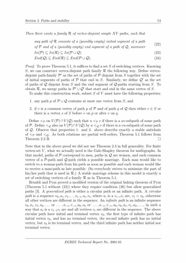
Then there exists a family R of vertex-disjoint simple XY -paths, such that

any path of R consists of a (possibly empty) initial segment of a path

of P and of a (possibly empty) end segment of a path of Q, moreover(22)

In(P) ⊆ In(R) ⊆ In(P ∪Q) (23)

End(Q) ⊆ End(R) ⊆ End(P ∪Q). (24)

Proof. To prove Theorem 5.1, it suffices to find a set S of switching vertices. KnowingS, we can construct vertex-disjoint path family R the following way. Define vertex-disjoint path-family P ′ as the set of paths of P disjoint from S together with the setof initial segments of paths of P that end in S. Similarly, we define Q′ as the setof paths of Q disjoint from S and the end segment of Q-paths starting from S. Toobtain R, we merge paths in P ′ ∪Q′ that start and end in the same vertex of S.

To make this construction work, subset S of V must have the following properties:

1. any path p of P ∪Q contains at most one vertex from S, and

2. if v is a common vertex of path p of P and of path q of Q then either v ∈ S orthere is a vertex s of S before v on p or after v on q.

Define <P on V (P)∩ V (Q) such that u <P v if there is a uv-subpath of some pathof P . Define <Q also on V (P)∩V (Q) by u <Q v if there is a vu-subpath of some pathof Q. Observe that properties 1. and 2. above describe exactly a stable antichainof <P and <Q. As both relations are partial well-orders, Theorem 5.1 follows fromTheorem 2.3 B.

Note that in the above proof we did not use Theorem 2.3 in full generality. For finitevertex-set V , what we actually need is the Gale-Shapley theorem for multigraphs. Inthat model, paths of P correspond to men, paths in Q are women, and each commonvertex of a P-path and Q-path yields a possible marriage. Each man would like toswitch to a woman-path from his path as soon as possible and each woman would liketo receive a man-path as late possible. (So everybody strives to minimize the part ofhis/her path that is used in R.) A stable marriage scheme in this model is exactly aset of switching vertices of a family R as in Theorem 5.1.

Brualdi and Pym proved a modified version of the original linking theorem of Pym(Theorem 5.1 without (22)) where they require condition (26) but allow generalizedpaths [3]. A generalized path is either a circular path or an infinite path. A circularpath is a sequence v0, a1, v1, . . . vt−1, at, vt, where ai is a vi−1vi arc, vt = v0, otherwiseall other vertices are different in the sequence. An infinite path is an infinite sequencev0, a1, v1, a2, . . . or . . . , a−1, v−1, a0, v0 or . . . , a−1, v−1, a0, v0, a1, v1, a2, . . . , in such away that ai is a vi−1vi arc and all vertices vi are different in the sequence. The abovecircular path have initial and terminal vertex v0, the first type of infinite path hasinitial vertex v0, and has no terminal vertex, the second infinite path has no initialvertex, but v0 is its terminal vertex, and the third infinite path has neither initial norterminal vertex.



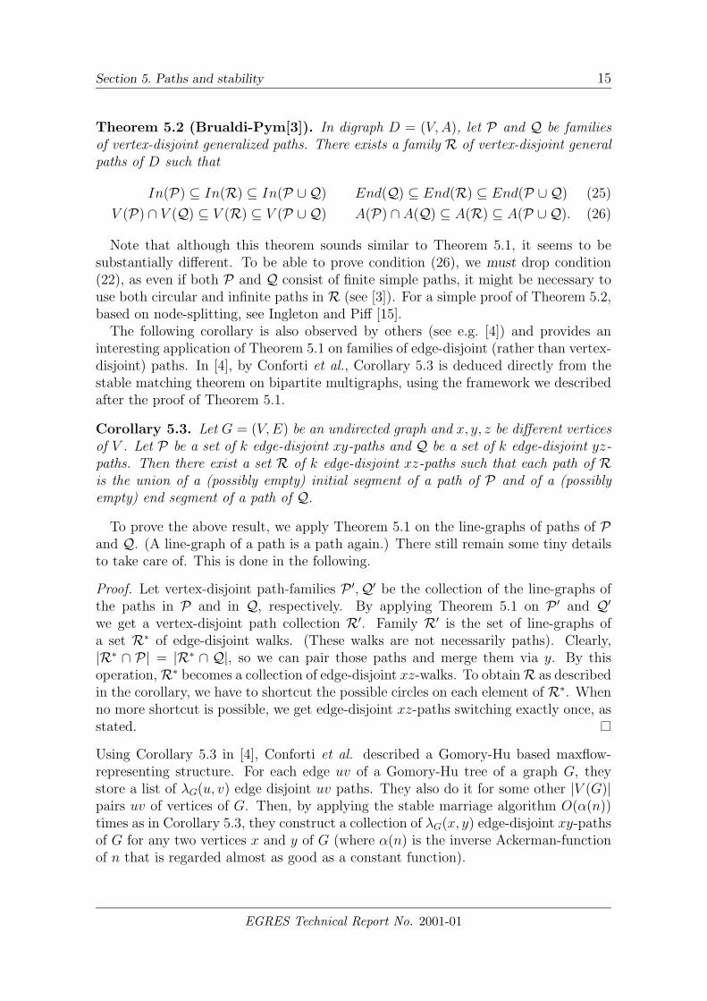
Theorem 5.2 (Brualdi-Pym[3]). In digraph D = (V,A), let P and Q be familiesof vertex-disjoint generalized paths. There exists a family R of vertex-disjoint generalpaths of D such that

In(P) ⊆ In(R) ⊆ In(P ∪Q) End(Q) ⊆ End(R) ⊆ End(P ∪Q) (25)

V (P) ∩ V (Q) ⊆ V (R) ⊆ V (P ∪Q) A(P) ∩ A(Q) ⊆ A(R) ⊆ A(P ∪Q). (26)

Note that although this theorem sounds similar to Theorem 5.1, it seems to besubstantially different. To be able to prove condition (26), we must drop condition(22), as even if both P and Q consist of finite simple paths, it might be necessary touse both circular and infinite paths in R (see [3]). For a simple proof of Theorem 5.2,based on node-splitting, see Ingleton and Piff [15].

The following corollary is also observed by others (see e.g. [4]) and provides aninteresting application of Theorem 5.1 on families of edge-disjoint (rather than vertex-disjoint) paths. In [4], by Conforti et al., Corollary 5.3 is deduced directly from thestable matching theorem on bipartite multigraphs, using the framework we describedafter the proof of Theorem 5.1.

Corollary 5.3. Let G = (V,E) be an undirected graph and x, y, z be different verticesof V . Let P be a set of k edge-disjoint xy-paths and Q be a set of k edge-disjoint yz-paths. Then there exist a set R of k edge-disjoint xz-paths such that each path of Ris the union of a (possibly empty) initial segment of a path of P and of a (possiblyempty) end segment of a path of Q.

To prove the above result, we apply Theorem 5.1 on the line-graphs of paths of Pand Q. (A line-graph of a path is a path again.) There still remain some tiny detailsto take care of. This is done in the following.

Proof. Let vertex-disjoint path-families P ′,Q′ be the collection of the line-graphs ofthe paths in P and in Q, respectively. By applying Theorem 5.1 on P ′ and Q′we get a vertex-disjoint path collection R′. Family R′ is the set of line-graphs ofa set R∗ of edge-disjoint walks. (These walks are not necessarily paths). Clearly,|R∗ ∩ P| = |R∗ ∩ Q|, so we can pair those paths and merge them via y. By thisoperation,R∗ becomes a collection of edge-disjoint xz-walks. To obtainR as describedin the corollary, we have to shortcut the possible circles on each element of R∗. Whenno more shortcut is possible, we get edge-disjoint xz-paths switching exactly once, asstated.

Using Corollary 5.3 in [4], Conforti et al. described a Gomory-Hu based maxflow-representing structure. For each edge uv of a Gomory-Hu tree of a graph G, theystore a list of λG(u, v) edge disjoint uv paths. They also do it for some other |V (G)|pairs uv of vertices of G. Then, by applying the stable marriage algorithm O(α(n))times as in Corollary 5.3, they construct a collection of λG(x, y) edge-disjoint xy-pathsof G for any two vertices x and y of G (where α(n) is the inverse Ackerman-functionof n that is regarded almost as good as a constant function).


Section 6. Matroid-kernels 16

6 Matroid-kernels

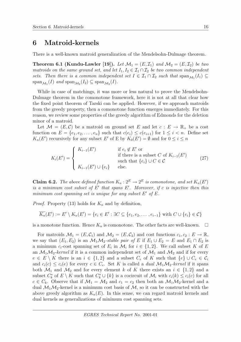
There is a well-known matroid generalization of the Mendelsohn-Dulmage theorem.

Theorem 6.1 (Kundu-Lawler [19]). Let M1 = (E, I1) and M2 = (E, I2) be twomatroids on the same ground set, and let I1, I2 ∈ I1 ∩ I2 be two common independentsets. Then there is a common independent set I ∈ I1 ∩ I2 such that spanM1

(I1) ⊆spanM1

(I) and spanM2(I2) ⊆ spanM2

(I).

While in case of matchings, it was more or less natural to prove the Mendelsohn-Dulmage theorem in the comonotone framework, here it is not at all that clear howthe fixed point theorem of Tarski can be applied. However, if we approach matroidsfrom the greedy property, then a comonotone function emerges immediately. For thisreason, we review some properties of the greedy algorithm of Edmonds for the deletionminor of a matroid.

Let M = (E, C) be a matroid on ground set E and let c : E → R+ be a costfunction on E = {e1, e2, . . . , en} such that c(ei) ≤ c(ei+1) for 1 ≤ i < n. Define setKn(E ′) recursively for any subset E ′ of E by K0(E

′) = ∅ and for 0 ≤ i ≤ n

Ki(E′) =

Ki−1(E

′) if ei 6∈ E ′ orif there is a subset C of Ki−1(E

′)such that {ei} ∪ C ∈ C

Ki−1(E′) ∪ {ei} else.

(27)

Claim 6.2. The above defined function Kn : 2E → 2E is comonotone, and set Kn(E ′)is a minimum cost subset of E ′ that spans E ′. Moreover, if c is injective then thisminimum cost spanning set is unique for any subset E ′ of E.

Proof. Property (13) holds for Kn and by definition,

Kn(E ′) := E ′ \Kn(E ′) = {ei ∈ E ′ : ∃C ⊆ {e1, e2, . . . , ei−1} with C ∪ {ei} ∈ C}

is a monotone function. Hence Kn is comonotone. The other facts are well-known.

For matroids M1 = (E, C1) and M2 = (E, C2) and cost functions c1, c2 : E → R,we say that (E1, E2) is an M1M2-stable pair of E if E1 ∪ E2 = E and E1 ∩ E2 isa minimum ci-cost spanning set of Ei in Mi for i ∈ {1, 2}. We call subset K of Ean M1M2-kernel if it is a common independent set of M1 and M2 and if for everye ∈ E \ K there is an i ∈ {1, 2} and a subset Ce of K such that {e} ∪ Ce ∈ Ciand ci(c) ≤ ci(e) for every c ∈ Ce. Set K is called a dual M1M2-kernel if it spansboth M1 and M2 and for every element k of K there exists an i ∈ {1, 2} and asubset C∗k of E \K such that C∗k ∪ {k} is a cocircuit of Mi with ci(k) ≤ ci(c) for allc ∈ Ck. Observe that if M1 = M2 and c1 = c2 then both an M1M2-kernel and adual M1M2-kernel is a minimum cost basis of M, so it can be constructed with theabove greedy algorithm as Kn(E). In this sense, we can regard matroid kernels anddual kernels as generalizations of minimum cost spanning sets.


Section 6. Matroid-kernels 17

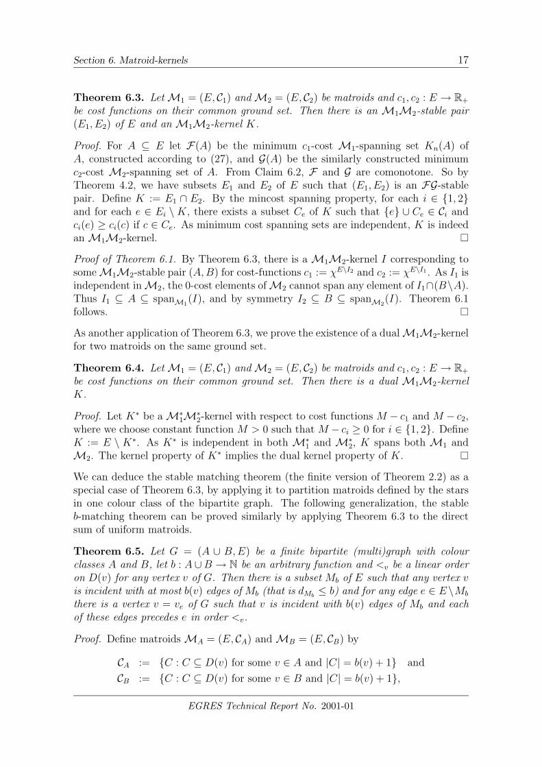
Theorem 6.3. LetM1 = (E, C1) andM2 = (E, C2) be matroids and c1, c2 : E → R+

be cost functions on their common ground set. Then there is an M1M2-stable pair(E1, E2) of E and an M1M2-kernel K.

Proof. For A ⊆ E let F(A) be the minimum c1-cost M1-spanning set Kn(A) ofA, constructed according to (27), and G(A) be the similarly constructed minimumc2-cost M2-spanning set of A. From Claim 6.2, F and G are comonotone. So byTheorem 4.2, we have subsets E1 and E2 of E such that (E1, E2) is an FG-stablepair. Define K := E1 ∩ E2. By the mincost spanning property, for each i ∈ {1, 2}and for each e ∈ Ei \K, there exists a subset Ce of K such that {e} ∪ Ce ∈ Ci andci(e) ≥ ci(c) if c ∈ Ce. As minimum cost spanning sets are independent, K is indeedan M1M2-kernel.

Proof of Theorem 6.1. By Theorem 6.3, there is a M1M2-kernel I corresponding tosomeM1M2-stable pair (A,B) for cost-functions c1 := χE\I2 and c2 := χE\I1 . As I1 isindependent inM2, the 0-cost elements ofM2 cannot span any element of I1∩(B\A).Thus I1 ⊆ A ⊆ spanM1

(I), and by symmetry I2 ⊆ B ⊆ spanM2(I). Theorem 6.1

follows.

As another application of Theorem 6.3, we prove the existence of a dualM1M2-kernelfor two matroids on the same ground set.

Theorem 6.4. LetM1 = (E, C1) andM2 = (E, C2) be matroids and c1, c2 : E → R+

be cost functions on their common ground set. Then there is a dual M1M2-kernelK.

Proof. Let K∗ be aM∗1M∗

2-kernel with respect to cost functions M − c1 and M − c2,where we choose constant function M > 0 such that M − ci ≥ 0 for i ∈ {1, 2}. DefineK := E \ K∗. As K∗ is independent in both M∗

1 and M∗2, K spans both M1 and

M2. The kernel property of K∗ implies the dual kernel property of K.

We can deduce the stable matching theorem (the finite version of Theorem 2.2) as aspecial case of Theorem 6.3, by applying it to partition matroids defined by the starsin one colour class of the bipartite graph. The following generalization, the stableb-matching theorem can be proved similarly by applying Theorem 6.3 to the directsum of uniform matroids.

Theorem 6.5. Let G = (A ∪ B,E) be a finite bipartite (multi)graph with colourclasses A and B, let b : A∪B → N be an arbitrary function and <v be a linear orderon D(v) for any vertex v of G. Then there is a subset Mb of E such that any vertex vis incident with at most b(v) edges of Mb (that is dMb

≤ b) and for any edge e ∈ E\Mb

there is a vertex v = ve of G such that v is incident with b(v) edges of Mb and eachof these edges precedes e in order <v.

Proof. Define matroids MA = (E, CA) and MB = (E, CB) by

CA := {C : C ⊆ D(v) for some v ∈ A and |C| = b(v) + 1} and

CB := {C : C ⊆ D(v) for some v ∈ B and |C| = b(v) + 1},


Section 7. The kernel lattice 18

cost functions cA, cB : E → N by cA(e) = n, cB(e) = m for any edge e = uv of G,where u ∈ A, v ∈ B, and n is the height of e in <u, and m is the height of e in <v.Apply Theorem 6.3 on MA,MB, cA and cB. The resulted matroid-kernel K =: Mb

will be a common independent set, that is dMb≤ b, and the optimal spanning property

shows that for any element e ∈ E \Mb there is a vertex v of G such that v is incidentwith b(v) edges of Mb each preceding e in <v.

The matching Mb described in Theorem 6.5 is called a stable b-matching.

7 The kernel lattice

In what follows, we focus on two well-studied aspects of the stable matching problem:first, we show a generalization of the so called “lattice structure” of stable matchings,and then, in Section 8, we deduce linear descriptions of kernel-related polyhedra fromit. By this, we characterize among others the matroid generalization of the stablematching polytope described by Vande Vate [33] and Rothblum [28].

As we mentioned earlier, Blair in [2] proved that stable assignments in the many-to-many model of Theorem 2.6 form a lattice. To come over the fact that it is nottrue that stable configurations form a lattice for the natural meet and join operationson assignments, he introduced a partial order on stable assignments that turned outto be a lattice order. Namely, he defined A ≤F B for assignments A and B if eachfirm in the model of Theorem 2.6 would choose assignment A if all choices in A and Bwould be offered. That is, if for each firm f we have Wf (A) = Cf (Wf (A) ∪Wf (B)),where sets of workers Wf (A) and Wf (B) are assigned to firm f in assignments A andB, respectively. Below, we show how Blair’s theorem follows from the lattice subsetproperty of fixed points in Tarski’s theorem.

Lemma 7.1. Let F ,G : 2X → 2X be comonotone set functions with property (20). If(A,B) and (A′, B′) are FG-stable pairs with FG-kernels F(A) = G(B) = K, F(A′) =G(B′) = K ′ and if F(K ∪K ′) = K then (A ∪ A′, B ∩ B′) is an FG-stable pair thatcorresponds to K.

Proof. As A ∪ B = X = A′ ∪ B′, we have (A ∪ A′) ∪ (B ∩ B′) = X. On the otherhand,

A ∩ F(A ∪ A′) ⊆ F(A) = K

A′ ∩ F(A ∪ A′) ⊆ F(A′) = K ′ (28)

by property (14) of F , as A ⊆ A∪A′ and A′ ⊆ A∪A′. This means that F(A∪A′) =F(A ∪ A′) ∩ (A ∪ A′) ⊆ K ∪K ′ ⊆ A ∪ A′, hence

K = F(K ∪K ′) = F(A ∪ A′) (29)

by property (20) of F . From (28, 29), it follows that A′∩K ⊆ K ′, thus K ⊂ B′ holdsbecause K ⊆ A′ ∪B′. So we have that G(B) = K ⊆ B ∩B′ ⊆ B, and

G(B ∩B′) = G(B) = K, (30)



by property (20) of G.Finally, we show that (A ∪ A′) ∩ (B ∩ B′) = K. From (29, 30), it is clear that

K ⊆ (A ∪ A′) ∩ (B ∩B′). For the opposite inclusion, we use relation

K ′ ∩B = G(B′) ∩ (B ∩B′) ⊆ G(B ∩B′) = K,

where the inclusion holds by property (14) of G, and the last equation by (30). Thismeans that

(A ∪ A′) ∩ (B ∩B′) = [A ∩ (B ∩B′)] ∪ [A′ ∩ (B ∩B′)] = (K ∩B′) ∪ (K ′ ∩B) ⊆ K.

From Lemma 7.1, we can give a simple explanation for the “opposition of commoninterest”, a property observed by Roth in [26]. If, for FG-kernels K and K ′ we haveF(K ∪K ′) = K, then, according to Lemma 7.1, there are FG-stable pairs (A′, B′) ≤(A∗, B∗) that correspond to K ′ and K, respectively. In particular, G(B∗) = K andG(B′) = K ′ and B∗ ⊆ B′. By property (20), from G(B′) = K ′ ⊆ K ∪ K ′ ⊆ B′ weget that G(K ∪ K ′) = K ′. In Roth’s model it means that if each firm unanimouslyprefers stable assignment K to K ′ , then each worker prefers K ′ to K.

To prove Blair’s theorem, we introduce a binary relation on FG-kernels for comono-tone functions F ,G : 2X → 2X . For FG-kernels K and K ′ we say that K ′ ≤FG K ifF(K ∪K ′) = K. Recall that we have defined on 2X × 2X a lattice order < by (17)and lattice operations ∧ and ∨ by (18).

Theorem 7.2 (Blair [2]). Let F ,G : 2X → 2X be comonotone set-functions withproperty (20). Then relation <FG is a lattice order on FG-kernels.

Proof. To prove that <FG is a lattice order, it is enough to show by Lemma 7.1 thatequivalence relation on FG-stable pairs defined by

(A,B) ∼ (A′, B′) if F(A) = F(A′) (31)

(that is if the corresponding FG-kernels are the same) is compatible with latticeoperations ∧FG,∨FG of the lattice of FG-stable pairs. Let FG-stable pairs (A′1, B

′1) ∼

(A′′1, B′′1 ) correspond to FG-kernel K1 and FG-stable pairs (A′2, B

′2) ∼ (A′′2, B

′′2 ) to

FG-kernel K2. As F and G have symmetric role and ∧FG = ∨GF , it is enough toprove compatibility for the join, that is

(A′, B′) := (A′1, B′1) ∨FG (A′2, B

′2) ∼ (A′′1, B

′′1 ) ∨FG (A′′2, B

′′2 ) =: (A′′, B′′).

By applying Lemma 7.1 on GF -stable pairs (B′1, A′1) and (B′′1 , A

′′1) and on (B′2, A

′2)

and (B′′2 , A′′2), we find GF -stable pairs

(B1, A1) := (B′1 ∪B′′1 , A′1 ∩ A′′1) = (B′1, A′1) ∨GF (B′′1 , A

′′1) ∼ (B′1, A

′1) and

(B2, A2) := (B′2 ∪B′′2 , A′2 ∩ A′′2) = (B′2, A′2) ∨GF (B′′2 , A

′′2) ∼ (B′2, A

′2).

Define FG-stable pair (A,B) := (A1, B1) ∨FG (A2, B2) and corresponding FG-kernelK := F(A). By definition, (A,B) ≤ (A′, B′) and (A,B) ≤ (A′′, B′′).



Using property (20), we get from F(A) = K ⊆ K1 ∪ K ⊂ A and F(A) = K ⊆K2 ∪K ⊂ A that K = F(K ∪K1) and K = F(K ∪K2). Hence by Lemma 7.1, wesee that both

(A,B) ∨ (A′1, B′1) ∨ (A′2, B

′2) = (A ∪ A′1 ∪ A′2, B ∩B′1 ∩B′2) and (32)

(A,B) ∨ (A′′1, B′′1 ) ∨ (A′′2, B

′′2 ) = (A ∪ A′′1 ∪ A′′2, B ∩B′′1 ∩B′′2 ) (33)

are FG-stable pairs with corresponding FG-kernel K. This means that (32) and (33)describe (A′, B′) and (A′′, B′′), respectively.

Next we generalize the sublattice property of bipartite stable matchings. Our aims areconditions that imply that the lattice subset of FG-stable pairs in Theorem 4.2 andthe lattice subset of fixed points in Theorem 3.1 is a sublattice. For a finite groundset X, we call function f : 2X → 2X strongly monotone if f is monotone and f hasthe subcardinal property of rank functions of matroids. Recall, that f is subcardinalif

|f(B) \ f(A)| ≤ |B \ A| (34)

for any A ⊆ B ⊆ X. Function f is increasing if

A ⊆ B ⊆ X implies |f(A)| ≤ |f(B)| . (35)

Note that if comonotone function F = Kn is coming from (27) then |F(A)| = rank(A),hence F is increasing. Also, the increasing property implies (20) for comonotonefunctions. We shall exhibit a link between strongly monotone functions, the sublatticestructure of fixed points of monotone functions and increasing comonotone functions.

First we give a sufficient condition for a monotone function on subset-lattices sothat the lattice subset of its fixed points is a sublattice.

Theorem 7.3. If f : 2X → 2X is a strongly monotone function for a finite set X,then fixed points of f form a nonempty sublattice of (2X ,∩,∪).

Proof. By Theorem 3.1, the set of fixed points is nonempty. Assume that f(A) = Aand f(B) = B. By monotonicity, A ∩ B = f(A) ∩ f(B) ⊇ f(A ∩ B) and A ∪ B =f(A) ∪ f(B) ⊆ f(A ∪B). By property (34),

|A \ (A ∩B)| ≥ |f(A) \ f(A ∩B)| ≥ |A \ A ∩B| and

|(A ∪B) \ A| ≥ |f(A ∪B) \ f(A)| ≥ |(A ∪B) \ A|,

hence there must be equality throughout. In particular, f(A ∩ B) = A ∩ B andf(A ∪B) = A ∪B.

The following link between strongly monotone and increasing comonotone functionsis crucial for the lattice property of FG-kernels.

Lemma 7.4. If function F : 2X → 2X is increasing and comonotone then F isstrongly monotone.



Proof. We have seen in (12) that function F is monotone. If A ⊆ B then

|F(B) \ F(A)| = |F(B)| − |F(A)| = |B \ F(B)| − |A \ F(A)| =|B| − |F(B)| − |A|+ |F(A)| ≤ |B| − |A| = |B \ A|.

Based on Lemma 7.4, we give a sufficient condition for the property that stable pairsin Theorem 4.2 form a sublattice. Recall that we have defined lattice order < by (17)and lattice operations ∧ and ∨ by (18) on 2X × 2X .

Theorem 7.5. If X is a finite ground set, F ,G : 2X → 2X are increasing comonotonefunctions then FG-stable pairs form a nonempty, complete sublattice of (2X×2X ,∧,∨).

Proof. We use the construction in the proof of Theorem 4.2. There we saw thatFG-stable pairs are exactly the fixed points of f(A,B) := (X \ G(B), X \ F(A)),defined in (19). It means that (A,B) is FG-stable if and only if B = X \ F(A) andA = f ′(A) := X \ G(X \ F(A)). Hence it is enough to prove that the fixed points off ′ form a nonempty sublattice of (2X ,∩,∪).

If A ⊆ B ⊆ X, then F(A) ⊆ F(B) by monotonicity of F . Hence X\G(X\F(A)) ⊆X \ G(X \ F(B)), by monotonicity of G. So f ′ is monotone.

From the subcardinal property (34) of F and G

|f ′(B) \ f ′(A)| = |[X \ G(X \ F(B))] \ [X \ G(X \ F(A))]| == |G(X \ F(A)) \ G(X \ F(B))| ≤≤ |[X \ F(A)] \ [X \ F(B)]| == |F(B) \ F(A)| ≤ |B \ A|.

Hence f ′ is strongly monotone, and its fixed points form a nonempty, complete sublat-tice of (2X ,∩,∪). That is, FG-stable pairs determine a nonempty, complete sublatticeof (2X × 2X , <).

Theorem 7.5 is equivalent with saying that if F and G are increasing comonotonefunctions, then <FG defines a lattice LFG on FG-kernels with lattice operations givenby K1 ∨FG K2 := (A1 ∪ A2) ∩ (B1 ∩ B2) and K1 ∧FG K2 := (A1 ∩ A2) ∩ (B1 ∪ B2).Identity χA1∩B1 + χA2∩B2 = χ(A1∪A2)∩(B1∩B2) + χ(A1∩A2)∩(B1∪B2) is easy to check, so wesee that

χK + χL = χK∨L + χK∧L (36)

holds for any FG-kernels K1 and K2. Observe, that K is an FG-kernel if and only ifit is a GF -kernel, and note that <GF=<−1

FG, thus K1 ∨FG K2 = K1 ∧GF K2. In whatfollows, we might omit the subscript in the lattice operations or in the partial orderwhen it does not cause ambiguity and clearly comes from FG-stability.

Corollary 7.6. Let F and G be increasing comonotone functions. If K1, K2, . . . , Kn

are FG-kernels then |Ki| = |Kj| and∨i∈[n]Ki = F(

⋃i∈[n]Ki) and

∧i∈[n]Ki =

G(⋃i∈[n]Ki).



Proof. Assume that FG-stable pairs (Ai, Bi) and (Aj, Bj) correspond to FG-kernelsKi and Kj, respectively. From the increasing property (35) of F and G, we get that|Ki| = |F(Ai)| ≤ |F(Ai ∪ Aj)| = |Ki ∨Kj| = F(Bi ∩ Bj)| ≤ |G(Bi)| = |Ki|. Hence|Ki| = |Ki ∨Kj| = |Kj|.

Let A :=⋃i∈[n]Ai and K :=

⋃i∈[n]Ki. Clearly,

∨i∈[n]Ki ⊆ K ⊆ A. Property (14)

of F yields∨i∈[n]Ki = F(A)∩K ⊆ F(K). On the other hand, the increasing property

of F implies that |F(K)| ≤ |F(A)| = |∨i∈[n]Ki|. Thus F(

⋃i∈[n]Ki) =

∨i∈[n]Ki.

Similarly, it follows that G(⋃i∈[n]Ki) =

∧i∈[n]Ki.

Corollary 7.6 can be regarded as a generalization of the “consensus property” observedby Roth in [26]. The fact that F(

⋃Ki) is an FG-kernel can be translated into the

language of his model the following way. If we fix a set S of stable assignment andeach firm f freely selects its employees from those workers who are assigned to f inat least one stable assignment of S then a stable assignment is defined.

From now on, we use k to denote the common size of FG-kernels for increasingcomonotone functions F and G. Theorem 7.5 implies the following observation onmatroids:

Corollary 7.7. If M1,M2 are matroids on the same ground set, c1, c2 are injectivecost functions, and K1, K2 are M1M2-kernels, then spanMi

(K1) = spanMi(K2) for

i ∈ {1, 2}.

Proof. Choose M1M2-stable pairs (A1, B1) and (A2, B2) such that Ki = Ai ∩ Bi fori ∈ {1, 2}. By Theorem 7.5, K1∨K2 = (A1∪A2)∩ (B1∩B2) is both a minimal c1-costindependent set spanning A1 ∪ A2 and a minimal c2-cost independent set spanningB1 ∩B2. Clearly, for i, j ∈ {1, 2}

spanMi(Kj) = spanMi

(Aj) ⊆ spanMi(A1 ∪ A2) = spanMi

(K1 ∨K2)

hence spanMi(K1) ⊇ spanMi

(K1∨K2) ⊆ spanMi(K2). From |K1| = |K1∨K2| = |K2|

there must be equality all way through.

Corollary 7.7 explains a well-known fact in the one-to-many assignment model. Wementioned in Section 2 that those colleges in the student-to-college assignment modelthat cannot fill up their quota in some stable assignment receive the very same set ofstudents in any stable assignment. To prove this, recall that we remarked earlier thatthe existence of a stable scheme is a special case of Theorem 6.3 for partition matroidM1 and matroid M2 that is a direct sum of uniform matroids. In M1, we partitionthe edge set along the stars of students, for M2 the partition is given by the starsof colleges. A student star has rank 1 in M1, and the rank of a college star is thesame as the b-value of the particular college. So, if for stable b-matching Mb we haveb(u) > dMb

(u), then in the star of u only the edges of Mb are spanned in M2 by Mb,hence D(u)∩Mb = D(u)∩M ′

b for any other stable b-matching M ′b. As a special case,

we also proved that in the original marriage model no matter which stable marriagescheme is chosen, always the same persons get married.


Section 8. Kernel polyhedra 23

8 Kernel polyhedra

For comonotone functions F and G on the same ground set X and for subset M ofX, let us denote by

BFG := {B ⊆ X : B ∩K 6= ∅ for any K ∈ KFG}AFG := {A ⊆ X : |A ∩K| ≤ 1 for any member K of KFG}MFG := X \

⋃KFG

CM := cone{χ{e} : e ∈M} = {x ∈ RX+ : xe = 0 for e ∈ X \M}

the blocker and antiblocker of KFG, the set of non-kernel elements and the projectionof the positive orthant to R

M , respectively. (Recall that KFG denotes the set ofFG-kernels.)

Define further

PKFG := conv{χK : K ∈ KFG} (37)

CKFG := cone{χK : K ∈ KFG} = {λ · x : λ ∈ R+, x ∈ PKFG}P↑KFG := PKFG + R

X+ = {x+ y : x ∈ PKFG , y ≥ 0} (38)

P↓KFG := (PKFG − RX+ ) ∩ R

X+ = {x− y : x ∈ PKFG , y ≥ 0} ∩ R

|X|+ (39)

P↑BFG := {χB : B ∈ BFG}↑ = {x+ y : x ∈ conv{χB : B ∈ BFG}, y ≥ 0} (40)

P↓AFG := {χA : A ∈ AFG}↓ + CMFG =

= CMFG + {x− y : x ∈ conv{χA : A ∈ AFG}, y ≥ 0} ∩ RX+ (41)

the FG-kernel polytope, the FG-kernel cone, the dominant of the FG-kernel poly-tope, the submissive of the kernel polytope, the FG-blocker polyhedron and the FG-antiblocker polyhedron, respectively. We are going to characterize these polyhedrain terms of linear constraints. For P↑BFG and P↓AFG we apply the theory of latticepolyhedra and for the rest we use the theory of (anti)blocking polyhedra.

To state the Hoffman-Schwartz theorem, a basic result on lattice polyhedra, weneed to formulate some assumptions. Fix a ground set X and a family L of subsetsof X. A partial order < on L is called consistent if A∩C ⊆ B holds for any membersA,B,C of L with A < B < C. Family L is a clutter if there is a consistent latticeorder < on L with lattice operations ∧ and ∨ such that

χA + χB = χA∧B + χA∨B

holds for any members A,B of L.

Theorem 8.1 (Hoffman-Schwartz [14]). Let L ⊆ 2X be a clutter for consistentlattice order < and lattice operations ∧,∨ and let d : X → N ∪ {∞} be and arbitraryfunction. If r : L → N is submodular then system

{x ∈ RX : 0 ≤ x ≤ d, x(A) ≤ r(A) for any A ∈ L} (42)



is TDI.If r : L → N is supermodular then system

{x ∈ RX : 0 ≤ x ≤ d, x(A) ≥ r(A) for any A ∈ L} (43)

is TDI.

(Here, r : L → N is submodular if r(A) + r(B) ≥ r(A∧B) + r(A∨B) holds for anyA,B ∈ L; r is supermodular if the reverse inequality is true.)

Next we observe that Theorem 8.1 is relevant in our setting.

Observation 8.2. If F ,G : 2X → 2X are increasing comonotone functions thenfamily KFG of FG-kernels is a clutter for lattice order <FG.

Proof. If K1 <FG K2 <FG K3 for K1, K2, K3 ∈ KFG then by Lemma 7.1, there arecorresponding FG-stable pairs (A1, b1) <FG (A2, B2) <FG (A3, B3). By (13) and (14),K1 ∩K3 = F(A1)∩F(A3) ⊆ A1 ∩F(A3) ⊆ A2 ∩F(A3) ⊆ F(A2) = K2, hence latticeorder <FG is consistent. By (36), KFG is a clutter.

By applying the Hoffman-Schwartz theorem on KFG, we get the following.

Theorem 8.3. If FG are increasing comonotone functions on ground set X then

P↑BFG = {x ∈ RX : x ≥ 0 and x(K) ≥ 1 for any K ∈ KFG} and (44)

P↓AFG = {x ∈ RX : x ≥ 0 and x(K) ≤ 1 for any K ∈ KFG}. (45)

Proof. Obviously, the polyhedra on the left hand side of (44,45) are the integer hullsof the polyhedra described by right hand sides.

By Observation 8.2, KFG is a clutter. Let d(v) := ∞ and r(K) := 1 for all v ∈ Xand K ∈ KFG. Clearly, r is sub- and supermodular. By Theorem 8.1, linear systemsin (44,45) are TDI, hence the polyhedra on the right hand sides are integer.

We introduce some basic notions from the theory of blocking and antiblocking poly-hedra to be able to describe other kernel-related polyhedra.

Polyhedron P ⊆ Rd+ is a blocking type polyhedron if P = P + R

d+, and it is an

antiblocking type polyhedron if P = Rd+∩ (P + R

d−). Any finite subset H of R

d+ defines

a blocking and an antiblocking polyhedron by

H↑ := conv(H) + Rd+ and H↓ := R

d+ ∩ (conv(H) + R

d−),

respectively. For a polyhedron P

B(P ) := {x ∈ Rd+ : xTy ≥ 1 for all y ∈ P} and

A(P ) := {x ∈ Rd+ : xTy ≤ 1 for all y ∈ P}

are the blocking and antiblocking polyhedron of P , respectively. As suggested by thename, if P is a polyhedron then both A(P ) and B(P ) are polyhedra.



Theorem 8.4 (Fulkerson [8, 9, 10]). If P is a blocking type polyhedron then B(P )is a blocking type polyhedron and P = B(B(P )). If P is an antiblocking type polyhe-dron then A(P ) is an antiblocking type polyhedron and P = A(A(P )). Furthermore,

B({x1, x2, . . . , xn}↑) = {y ∈ Rd+ : yTxi ≥ 1 for i ∈ [n]} (46)

A({x1, x2, . . . , xn}↓) + CM = {y ∈ Rd+ : yTxi ≤ 1 for i ∈ [n] and

y(m) = 0 for m ∈M} (47)

for any n ∈ N, subset M of [d] and elements xi (i ∈ [n]) of Rd+.

With these tools, we can give the following descriptions for our kernel polyhedra.

Theorem 8.5. If FG are increasing comonotone functions on ground set X and k isthe common size of FG-kernels then

P↑KFG = {x ∈ RE : x ≥ 0, x(B) ≥ 1 for B ∈ BFG} , (48)

P↓KFG = {x ∈ RE : x ≥ 0, x(MFG) = 0 and x(A) ≤ 1 for any A ∈ KFG} , (49)

PKFG = {x ∈ RE : x ≥ 0, 1Tx ≤ k, x(B) ≥ 1 for B ∈ BFG} , (50)

PKFG = {x ∈ RE : x ≥ 0, x(MFG) = 0, 1Tx ≥ k, x(A) ≤ 1 for A ∈ AFG} ,(51)

CKFG = {x ∈ RE : x ≥ 0, k · x(B) ≥ 1Tx for B ∈ BFG} , and (52)

CKFG = {x ∈ RE : x ≥ 0, x(MFG) = 0, k · x(A) ≤ 1Tx for A ∈ AFG} . (53)

Proof. By (44) and (46), P↑BFG = B(P↑KFG). From Theorem 8.4, we get that P↑KFG =

B(P↑BFG), and (48) follows from (46). Similarly, P↓AFG = A(P↓KFG) from (45) and

(47). Theorem 8.4 implies that P↓KFG = A(P↓AFG), so (49) follows from (47). As eachFG-kernel has the same size k, (50) follows directly from (48), and (51) from (49).

Clearly, both cones C and C ′ described on the right hand sides of (52) and (53)contain CKFG . Let x ≥ 0 be a vector outside CKFG , and λ = k

1T x. Then 1T (λ · x) = k

and λ · x 6∈ P↑KFG ∪ P↓KFG , hence there is a member B of BFG such that λ · x(B) < 1

and if x(MFG) = 0 then there is a member A of AFG with λ · x(A) > 1. This meansthat k · x(B) < k

λ= 1Tx and k · x(A) > k

λ= 1Tx. Thus x 6∈ C and x 6∈ C ′, justifying

(52) and (53).

Note that we gave two different descriptions for both PKFG and CKFG . Apart fromthe nonnegativity conditions, there is no constraint that appears in both of the de-scription. In particular, this means that CKFG can neither be full dimensional nor1-codimensional. It is also interesting to observe that the linear description by VandeVate [33] and Rothblum [28] for the convex hull of bipartite stable matchings is relatedto (50).

Theorem 8.6 (Rothblum [28], see also Vande Vate [33]). Let G = (V,E) be afinite bipartite graph and for each v ∈ V let <v be a linear order on D(v). Defineφ(e) := {f ∈ E : f ≤u e or f ≤v e} for edge e = uv ∈ E. Then

conv{χF : F ⊆ E is a stable matching of G} = (54)

{x : 0 ≤ x ∈ RE, x(D(v)) ≤ 1 for v ∈ V, x(φ(e)) ≥ 1 for e ∈ E}.



In (54), conditions x(D(v)) ≤ 1 are special cases of conditions of type x(A) ≤ 1of (51) and together with nonnegativity of x, these are responsible for any solution xis a convex combination of bipartite matchings. Constraints x(φ(e)) ≥ 1 are specialcases of x(B) ≥ 1 type constraints in (50). In fact, as 1Tx ≥ k for any x ∈ P↑KFG and

1Tx ≤ k for any x ∈ P↓KFG , we have that PKFG = P↑KFG ∩ P↓KFG . It follows that

PKFG = {x ∈ RE : x ≥ 0, x(B) ≥ 1 for B ∈ BFG,

x(A) ≤ 1 for A ∈ AFG} , (55)

because for a vector x of the right hand side, define x′ by zeroing the coordinates ofx that correspond to elements e ∈MFG and add x(MFG) to some other coordinate ofx. It is easy to check that x′ ∈ P↑KFG ∩P

↓KFG , hence 1Tx′ = k. But then x ∈ P↑KFG can

only hold if x = x′, that is, condition x(MFG) = 0 automatically holds in (55). Notethat characterization (55) resembles very much to (54).

Another interesting question whether linear descriptions (48-53) are good character-izations, that is, whether the separation problem over those polyhedra can be solvedefficiently. The answer is yes, and a possible way for P↑KFG is explained in [7].

Finally, to contrast Theorem 8.5, we prove that it is NP-complete to decide whethera particular element of the ground set can belong to some stable antichain or not. Itmeans that unless P=NP, it is necessary to have some extra assumption (like theincreasing property) on the comonotone functions to hope for a good characterizationof the corresponding FG-kernel polytope, PKFG . We will use Observation 4.3, theonly example of non-increasing comonotone function we have seen so far.

Theorem 8.7. If undirected graph G = (V,E) and k ∈ N are given then it is possibleto construct partial orders < and <′ and an element s of their common ground-set Xin time polynomial in |V |, such that s belongs to a stable antichain of < and <′ if andonly if G contains an independent set of size k.

Proof. We may assume k ≤ |V |, otherwise the theorem is trivial. Otherwise let

X := {s} ∪ {aj, a′j : 1 ≤ j ≤ k} ∪ {vj, v′j : v ∈ V, 1 ≤ j ≤ k}.

Partial orders < and <′ are determined by

aj < s, uj < v′j, wl < v′j, vj < a′j

a′j <′ s, u′j <

′ vj, w′l <′ vj, v′j <

′ aj

for 1 ≤ j ≤ k, 1 ≤ l ≤ k, j 6= l, u, v, w ∈ V , u 6= v and vw ∈ E or v = w.

IfG has an independent set I = {i1, i2, . . . , ik} ⊆ V of size k, then S := {s}∪{ijj, ijj

′:

1 ≤ j ≤ k} is a stable antichain of < and <′. On the other hand, if s belongs to astable antichain S then neither aj, nor a′j can belong to S. Thus for every j there

must exist elements ij and ej of V such that ijj, ejj

′ ∈ S. By stability ij = ej 6= il and

ijil 6∈ E for j 6= l, in other words I := {i1, i2, . . . , ik} is an independent set of G ofsize k.


References 27

As the decision problem whether there exists an independent set of size k in a graphis NP-complete, it is also NP-complete to solve the kernel-problem in Theorem 8.7.We give another reason why it is NP-complete to optimize kernels. For an undirectedgraph G = (V,E), function f : 2E → 2E, defined by f(E ′) = {e = uv ∈ E ′ :D(u)∪D(v) ⊆ E ′} for E ′ ⊆ E is monotone. Consider comonotone function F , definedby F(E ′) := E ′ \ f(E ′). It is easy to see that FF -stable pairs are (E(U), E(V \ U))where E(U) :=

⋃v∈U D(v) (for U ⊆ V ), and FF -kernels are exactly the edge-sets of

the form D(U), for some U ⊆ V . If it would be possible to separate over the kernelpolytope PFF , then (by the ellipsoid method) it would be possible to find a maximumcut of G in polynomial time. But this latter problem is NP-complete.

AcknowledgementHereby I acknowledge Ron Aharoni, Krzysztof Apt, Andras Biro, Andras Frank, BertGerards, Judith Keijsper, Romeo Rizzi, Lex Schrijver and Andras Sebo for their ideasand for the discussions on the topic.

References

[1] Garrett Birkhoff. Lattice Theory. American Mathematical Society, New York, N. Y.,revised edition, 1948.

[2] Charles Blair. The lattice structure of the set of stable matchings with multiple part-ners. Math. Oper. Res., 13(4):619–628, 1988.

[3] R. A. Brualdi and J. S. Pym. A general linking theorem in directed graphs. In Studies inPure Mathematics (Presented to Richard Rado), pages 17–29. Academic Press, London,1971.

[4] M. Conforti, R. Hassin, and R. Ravi. Reconstructing flow paths. submitted, 1999.

[5] Vincent P. Crawford and Elsie Marie Knoer. Job matching with heterogenous firmsand workers. Econometrica, 49:437–450, 1981.

[6] Tomas Feder. A new fixed point approach for stable networks and stable marriages. J.Comput. System Sci., 45(2):233–284, 1992. Twenty-first Symposium on the Theory ofComputing (Seattle, WA, 1989).

[7] Tamas Fleiner. Stable and crossing structures, August, 2000. PhD dissertation,http://www.renyi.hu/~fleiner.

[8] D. R. Fulkerson. Blocking polyhedra. In Graph Theory and its Applications (Proc.Advanced Sem., Math. Research Center, Univ. of Wisconsin, Madison, Wis., 1969),pages 93–112. Academic Press, New York, 1970.

[9] D. R. Fulkerson. Blocking and anti-blocking pairs of polyhedra. Math. Programming,1:168–194, 1971.

[10] D. R. Fulkerson. Anti-blocking polyhedra. J. Combinatorial Theory Ser. B, 12:50–71,1972.


References 28

[11] D. Gale and L.S. Shapley. College admissions and stability of marriage. Amer. Math.Monthly, 69(1):9–15, 1962.

[12] Fred Galvin. The list chromatic index of a bipartite multigraph. J. Combin. TheorySer. B, 63(1):153–158, 1995.

[13] Dan Gusfield and Robert W. Irving. The stable marriage problem: structure and algo-rithms. MIT Press, Cambridge, MA, 1989.

[14] A. J. Hoffman and D. E. Schwartz. On lattice polyhedra. In Combinatorics (Proc.Fifth Hungarian Colloq., Keszthely, 1976), Vol. I, pages 593–598. North-Holland, Am-sterdam, 1978.

[15] A. W. Ingleton and M. J. Piff. Gammoids and transversal matroids. J. CombinatorialTheory Ser. B, 15:51–68, 1973.

[16] Jr Kelso, Alexander S. and Vincent P. Crawford. Job matching, coalition formation,and gross substitutes. Econometrica, 50:1483–1504, 1982.

[17] Bronis law Knaster. Un theoreme sur les fonctions d’ensembles. Ann. Soc. Polon. Math.,6:133–134, 1928.

[18] Donald E. Knuth. Stable marriage and its relation to other combinatorial problems.American Mathematical Society, Providence, RI, 1997. An introduction to the math-ematical analysis of algorithms, Translated from the French by Martin Goldstein andrevised by the author.

[19] Sukhamay Kundu and Eugene L. Lawler. A matroid generalization of a theorem ofMendelsohn and Dulmage. Discrete Math., 4:159–163, 1973.

[20] Azriel Levy. Basic set theory. Springer-Verlag, Berlin, 1979.

[21] N. S. Mendelsohn and A. L. Dulmage. Some generalizations of the problem of distinctrepresentatives. Canad. J. Math., 10:230–241, 1958.

[22] J. S. Pym. The linking of sets in graphs. J. London Math. Soc., 44:542–550, 1969.

[23] J. S. Pym. A proof of the linkage theorem. J. Math. Anal. Appl., 27:636–638, 1969.

[24] Alvin E. Roth. The evolution of the labor market for medical interns and residents: Acase study in game theory. Journal of Political Economy, Y2(6):991–1016, 1984.

[25] Alvin E. Roth. Stability and polarization of intersts in job matching. Econometrica,52(1):47–57, 1984.

[26] Alvin E. Roth. Conflict and coincidence of interest in job matching: some new resultsand open questions. Math. Oper. Res., 10(3):379–389, 1985.

[27] Alvin E. Roth and Marilda A. Oliveira Sotomayor. Two-sided matching. CambridgeUniversity Press, Cambridge, 1990. A study in game-theoretic modeling and analysis,With a foreword by Robert Aumann.

[28] Uriel G. Rothblum. Characterization of stable matchings as extreme points of a poly-tope. Math. Programming, 54(1, Ser. A):57–67, 1992.


References 29

[29] B. Sands, N. Sauer, and R. Woodrow. On monochromatic paths in edge-coloureddigraphs. J. Combin. Theory Ser. B, 33(3):271–275, 1982.

[30] Alexander Schrijver. Theory of linear and integer programming. John Wiley & SonsLtd., Chichester, 1986. A Wiley-Interscience Publication.

[31] Ashok Subramanian. A new approach to stable matching problems. SIAM J. Comput.,23(4):671–700, 1994.

[32] Alfred Tarski. A lattice-theoretical fixpoint theorem and its applications. Pacific J. ofMath, 5:285–310, 1955.

[33] John H. Vande Vate. Linear programming brings marital bliss. Oper. Res. Lett.,8(3):147–153, 1989.


A fixed-point approach to stable matchings and some applications

Documents

Transcript of A fixed-point approach to stable matchings and some applications