A Five-Star Rating Scheme to Assess Application Seamlessness › system › files › swj951.pdf ·...

Undefined 0 (2014) 1–0 1IOS Press

A Five-Star Rating Scheme to AssessApplication SeamlessnessEditor(s): Name Surname, University, CountrySolicited review(s): Name Surname, University, CountryOpen review(s): Name Surname, University, Country

Timothy Lebo ∗,∗∗, Nicholas Del Rio, Patrick Fisher, and Chad SalisburyAir Force Research Laboratory, Information DirectorateRome, NY, USA

Abstract. Analytics is a widespread phenomenon that often requires analysts to coordinate operations across a variety of incom-patible tools. When incompatibilities occur, analysts are forced to configure tools and munge data, distracting them from theirultimate task objective. This additional burden is a barrier to our vision of seamless analytics, i.e. the use and transition of con-tent across tools without incurring significant costs. Our premise is that standardized semantic web technologies (e.g., RDF andOWL) can enable analysts to more easily munge data to satisfy tools’ input requirements and better inform subsequent analyticalsteps. However, although the semantic web has shown some promise for interconnecting disparate data, more needs to be doneto interlink user- and task-centric, analytic applications. We present five contributions towards this goal. First, we introduce anextension of the W3C PROV Ontology to model analytic applications regardless of the type of data, tool, or objective involved.Next, we exercise the ontology to model a series of applications performed in a hypothetical but realistic and fully-implementedscenario. We then introduce a measure of seamlessness for any ecosystem described in our Application Ontology. Next, weextend the ontology to distinguish five types of applications based on the structure of data involved and the behavior of the toolsused. By combining our 5-star application rating scheme and our seamlessness measure, we propose a simple Five-Star Theoryof Seamless Analytics that embodies tenets of the semantic web in a form which emits falsifiable predictions and which can berevised to better reflect and thus reduce the costs embedded within analytical environments.

Keywords: analytics, interoperability, Linked Data, semantics, evaluation

1. Introduction

Linked Data is a large, decentralized, and loosely-coupled conglomerate covering a variety of topical do-mains and slowly converging to use well-known vo-cabularies [1,2]. To more fully reap the benefits ofsuch diverse data, linked data analysts must employ anequally diverse array of analytical tools.

Meanwhile, the Visual Analytics community hasbeen forging a science of analytical reasoning andinteractive visual interfaces to facilitate analysis of

*Corresponding author. E-mail: [email protected]**DISTRIBUTION STATEMENT A. Approved for public re-

lease; distribution is unlimited. Case Number: 88ABW-2014-5577

“overwhelming amounts of disparate, conflicting, anddynamic information [3]." Although the communityhas produced a vast array of tools and techniques thatcould assist [4], it remains difficult to easily reusethose tools in evolving environments such as the worldof linked data analytics – perhaps because they rely onmore mundane representations that make it difficult toestablish and maintain connections across analyses.

Our work considers applications as an analyst’scontextualized use of a tool to suit a specific objec-tive. We focus on the more difficult kind of applica-tion where analysts use third-party tools to processthird-party data and thus have limited control on de-sign and behavior. Regardless of which community’sapproaches are adopted, the need to continually form

0000-0000/14/$00.00 c© 2014 – IOS Press and the authors. All rights reserved

2 T. Lebo et al. / Analytical Seamlessness

interconnections among the triad consisting of data,analyst, and tool remains a costly endeavor – and tobenefit from both visual analytics and linked data re-search, the costs need to be more clearly portrayed, as-sessed, and overcome.

Our hypothesis is that analysts are better able tochain applications together to support threads of anal-yses when tools:

1. declare their input semantics and2. provide their derived results as linked data.

With respect to declaring input semantics, the flexi-bility afforded by new APIs such as D3 [5] has resultedin a proliferation of “one-off” visualization tools thatinhibit low-cost reusability. These new visualizationsregularly assume specific input data formats about spe-cific topics that are not explicitly expressed. Withoutexplicit and formal input semantics, analysts are de-prived of a meaningful munging target and must fallback to rummaging through example input datasetsor inspecting source code to reconstruct the visualiza-tion’s implicit data requirements, which can consumeup to 80% of the analytical process [6].

With respect to providing results as linked data,even if analysts could easily reuse the near two-thousand cataloged D3 visualizations1, each visual-ization is a sink from the standpoint of an analyti-cal ecosystem. Results derived from previous applica-tions, including interactions and selections, are oftennot codified in forms that can reduce integration costsincurred by subsequent analyses that can benefit fromprevious results.

Our contributions and sectioning of this paper areillustrated in Figure 1. As shown at the bottom of thestack, Section 2 introduces an extension of the W3CPROV Ontology to model analytic applications regard-less of the type of data, tool, or objective involved.Section 3 exercises the ontology to model a series ofapplications performed in a hypothetical but realisticand fully-implemented scenario. Section 4 introducesa measure of seamlessness based on the cost of per-forming applications in ecosystems described usingour application ontology. Section 5 extends the appli-cation ontology to distinguish five types of applica-tions that comprise our five-star theory, which statesthat the structure of data and tools employed in ap-plications dictates the level of analytical seamlessness.

1http://christopheviau.com/d3list/ maintains a list of public D3 vi-sualizations. The current count as of December 10, 2014 was 1,897visualizations.

Ontology

Computation

Theory

Implementation

Use Case

Exemplar Analytical Scenario

(§ 3)

Exemplar EcosystemApplication Ontology - Core (§ 2)

5-Star Application Ontology (§ 5)

Seamlessness Scoring

(§ 4)

5-Star Theory(§ 5)

Related Work(§ 6)

Future Work(§ 7)

Fig. 1. A theory of seamless analytics comprises four elements thatare illustrated with an exemplar and realistic, implemented scenario.

wasInformedBy

used

used

PROV Responsibility

wasGeneratedBy

DαApplication α

DataD

Toolt {

Triad

Munging mMunging m

AnalystA

Fig. 2. Application Ontology Core is an extension of PROV. Appli-cations use tools to generate new datasets which could include vi-sualizations. Applications are informed by munging activities thattransform data representations. Figure 10 illustrates an extension tofurther distinguish among five types of applications.

Section 6 describes past work in the area of analyt-ical models and techniques for supporting interoper-ability in analytical environments. Finally, Section 7discusses future work before concluding in Section 8.

2. An Ontology of Analytical Applications

Our core Application Ontology (AO) provides aminimal set of concepts to describe an analytical step,herein known as an application; a complete threadof analysis can be chained together when subsequentapplications use materials from previous applications,as exemplified in Section 3. Application chains canthen be assessed using the seamlessness measure in-

T. Lebo et al. / Analytical Seamlessness 3

troduced in Section 4 and can be further distinguishedinto five sub-types using the constraints introduced inSection 5.

An application refers to an analyst’s contextualizeduse of some dataset within a tool to achieve some im-plicit objective, which contrasts prior work of mod-eling applications as a piece of software [7]. Our ap-plications are a kind of PROV Activity [8], definedas “something that occurs over a period of time andacts upon or with entities; it may include consuming,processing, transforming, modifying, relocating, using,or generating entities." An application associates threekey entities, which we refer to as the application triad:1) the dataset used, 2) the performing analyst who alsomost immediately benefited from the result, and 3) thetool that derived a result from the dataset. Figure 2 il-lustrates these relations using the PROV layout con-ventions2 – Dα is the result derived from dataset D byanalyst A with tool t during application α.

The distinguishing aspect of our AO is the focuson munging activities that may be required to suit adataset to a tool’s input requirements. This relation isalso shown in Figure 2 using PROV, but we further re-late munging activities as also being part of the ap-plication3. Munging, also known as wrangling [6], isthe imperfect manipulation of data into a usable form.Munging has been recognized in the field for decades4,yet continues to be a ubiquitous and costly problem[9]. We focus on munging because it persists and dom-inates as a cost factor for applications.

As shown in Figure 3, we establish seven sub-classes of munging and group them into three interme-diate super-classes. These intermediate classes (mun-dane, semantic, and trivial munging) are distinguishedaccording to a dichotomy that can be found within TimBerners-Lee’s Linked Data rating scheme [1]. Broadlyspeaking, Berners-Lee’s scale can be used to partitiondata into two groups: non-RDF and RDF. Let D[1,3]

denote the union of all data earning one, two, or threestars according to the popular scheme, and D[4,5] theunion of all four or five-star data. We call any datasetwithin D[1,3] “mundane" and any dataset within D[4,5]

“semantic," reflecting the perspective of the SemanticWeb and Linked Data communities that more highlyrated data are easier to use or inherently provide morevalue. Let the function tbl return the star rating of a

2http://www.w3.org/2011/prov/wiki/Diagrams3Using Dublin Core, http://purl.org/dc/terms/4The New Hacker’s Dictionary http://catb.org/

jargon/html/M/munge.html

shim: [1,3] → [1,3]

lift: [1,3] →

[4,5]

cast: [4,5] → [1,3]glean:

[1,3] → [4,5]

align: [4,5] → [4,5]

compute: [4,5] → [4,5]

D[1,3] D[1,3]

D[4,5] D[4,5]

Munging m

MundaneMunging

(High Cost)• shim• lift• cast

SemanticMunging

(Medium Cost)• align• compute

TrivialMunging

(Low Cost)• glean• conneg

Fig. 3. Munging activities defined in terms of the Tim Berners-Lee’slinked data scale. Not shown is content negotiation because it appliesto all data types (an ideal situation).

dataset, i.e., tbl(Ds) = s). The seven sub-classes ofmunging (shim, lift, cast, align, compute, glean, andconneg) are defined in terms of using5 data from eitherD[1,3] or D[4,5] and generating data from the same.

munge : {D[1,3], D[4,5]} 7→ {D[1,3], D[4,5]}

Mundane munges incur the highest cost and areshown in Figure 3 with heaviest edges. Semanticmunges are less expensive than mundane munges andare shown with medium weight lines. Finally, trivialmunges are the least expensive of all and are shownwith lightest lines. The abstract and coarse level cost isintended to reflect the ease at which data can be usedwithin and across applications.

2.1. Mundane Munging

Three kinds of munging activities are common inthat they all require the analyst to understand both thestructure and semantics of mundane datasets (D[1,3]).

Shimming (shim): generates D[1,3] from D[1,3]; it isany data transformation that does not involveRDF and is the kind of activity that the LinkedData community is working to ameliorate.

5We continue to follow PROV terminology to describe activities.

http://www.w3.org/2011/prov/wiki/Diagrams

http://purl.org/dc/terms/

http://catb.org/jargon/html/M/munge.html

http://catb.org/jargon/html/M/munge.html


Lifting (lift): generates D[4,5] from D[1,3]; it createsRDF from non-RDF and has occupied the LinkedData community’s attention for most6 of the pastdecade [10,11,12].

Casting (cast): generates D[1,3] from D[4,5]; it cre-ates mundane forms from RDF and, unfortu-nately, is regularly performed by many LinkedData applications today, typically by using SPARQLto create browser-friendly HTML or SVG.

2.2. Semantic Munging

Two kinds of munging activities are common in thatthey require the analyst to understand only the seman-tics of datasets (D[4,5]).

Aligning (align): generates D[4,5] from D[4,5]; it de-rives new relationships from RDF and can oftenbe achieved using ontological mappings [13].

Computing (comp): generates D[4,5] from D[4,5]; itderives new information from RDF that is it-self also expressed in RDF. While aligning is aspecial kind of computing, there are many otherkinds of computing that are not aligning. Com-puting is relatively less common in current prac-tice but can be found in a few works such asLinking Open Vocabularies7 and SPARQL-ES[14].

2.3. Trivial Munging

Two kinds of munging activities are common in thatthey do not require the analyst to understand any of thedataset’s structure or semantics.

Gleaning (glean): generates D[4,5] from D[1,3]; theGRDDL8 and RDFa recommendations are bothapproaches that can be used to glean RDF fromnon-RDF representations without the need forcontextual knowledge.

Content Negotiation (conneg): generatesD[1,5] fromD[1,5] and “refers to the practice of making avail-able multiple representations via the same URI.”9

When a mundane dataset can be gleaned, its embed-ded semantic content will be denoted using an expo-nent. For example, an RDFa dataset embedding four-

6http://triplify.org/challenge7http://lov.okfn.org/dataset/lov/8http://www.w3.org/TR/grddl/9http://www.w3.org/TR/webarch/

D1,1a

α1,1

D1,1

tbl(D1,1) = 3Satellite KML

shim: [1,3] → [1,3](Google Earth)

α1,2

D1,2

tbl(D1,2) = 1Google Earth Map

D1,0cast: [4,5] → [1,3]

(Amy)tbl(D1,0) = 5Amy’s Know.

D1,1

tbl(D1,1) = 3keywords

shim: [1,3] → [1,3](Google)

Fig. 4. Munges performed to the support the applications duringTask 1.

star RDF is expressed as 34; the HTML’s three-star rat-ing is denoted as the base while the four star rating ofthe RDF is denoted with the exponent. The schema forthe gleanable notation is therefore [1, 3][4,5]. The expo-nent representing the star rating of the semantic con-tent is returned when these datasets are gleaned, for ex-ample: tbl(glean(D34)) = 4. These kinds of datasetsare flexible and allow analysts to use tools that pro-cess either the mundane carrier data or the embeddedsemantic content.

3. An Analytical Scenario: Space Junk

This section presents a representative analysis mod-eled according to our application ontology presentedin the previous section. The analysis is centered onthe broad topic of Earth’s artificial satellites, e.g.,where they are, who launches them, and how they havechanged over time. As our analyst performs applica-tions and inspects generated results, she will incremen-tally and serendipitously gain insight, formulate newquestions, and perform subsequent applications.

In addition to exercising our application model, weuse this scenario to highlight certain munging “anti-patterns” that are representative of the state of prac-tice in both analytics and linked data disciplines. Theseanti-patterns increase the cost associated with generat-ing and reusing materials and in some cases directlyinfluence how analysts design their applications to mit-igate compatibility issues [9]. Particular, we focus ontwo anti-patterns that we name the “house top” and“hill slide,” which can be identified visually in prove-nance munge traces that zigzag between the semanticand mundane levels.

3.1. Task 1: Where are Earth’s Artificial Satellites?

Amy, a student enrolled in a physics course, is learn-ing about trajectories as applied to satellite launches

http://triplify.org/challenge

http://lov.okfn.org/dataset/lov/

http://www.w3.org/TR/grddl/

http://www.w3.org/TR/webarch/


and becomes curious about the extent of materiallaunched into space. Although her professor mentionsthere are more than 2,000 satellites launched by vari-ous countries, she remains curious about the locationof these satellites and seeks some visualizations to gainperspective.

3.1.1. Task 1, Application 1 (α1,1): GoogleWithout prior materials to work from, Amy per-

forms a Google search to find relevant informationabout satellite orbits. She stumbles upon a KML fileprovided by Analytical Graphics Inc. (AGI) 10 that de-scribes satellites known to be in orbit, their launchdates, launch sites, and ownership by country. Her re-sulting query response page is iconified in the top laneof Figure 4.

In terms of munging, Amy relies on her existingknowledge of satellites to formulate a search query,also shown in the top lane of Figure 4. Dataset D1,0

represents Amy’s cognitive model [15] that is castedinto a mundane sequence of keywords D1,1a. We con-sider cognitive models as a kind of semantic data(i.e.,[4, 5]) since both embody interconnections amongconcepts, despite the fact that cognitive models cannever be fully embodied by a dataset. Amy then usesGoogle to shim her keywords into a results page thatcontains the AGI KML dataset D1,1 that satisfies hercriteria.

When analysts cast semantic data to the mundanelevel, they “fork” the analysis into two parallel threads.Upon casting, explicit interconnections maintained atthe semantic level are lost or become implicit and canonly be maintained within analysts’ cognitive models.As analysts continue to derive mundane results, theircognitive models must adapt in order to maintain thecorrespondence between the threads that parallel at se-mantic and mundane levels. If analysts eventually wantto unify the two threads, by lifting back to the semanticlevel, they will have to rely on their burdened cognitivemodels to reconstitute the connections lost at the datalevel, thereby duplicating effort and wasting resources.These casts can be seen in the remaining applications.

3.1.2. Task 1, Application 2 (α1,2): Google EarthNow that Amy has a relevant KML file, she uses

Google Earth to view it as an interactive geospatialview that plots the location of satellites, as iconified atthe bottom lane of Figure 4. The resulting interactivemap is littered with many satellites, providing Amy

10http://adn.agi.com/SatelliteDatabase/KmlNetworkLink.aspx

with some perspective regarding the quantity of satel-lites in orbit.

When analysts cast semantic data to mundanedatasets and continue to work at the mundane level,the hill slide anti-pattern can be observed. Visually,hill slides can be identified by a downward slope (i.e.,a cast) from the semantic level to the mundane level,followed by a series of shims as shown in the bottomlane of Figure 4. Using results generated by hill slidesincurs higher costs because shims and lifts would berequired to return to the semantic level. In terms ofmunging, Amy continues to hill slide and uses GoogleEarth to shim the mundane KML satellite data (D1,1)data to mundane pixels (D1,2), shown in the bottomlane of Figure 4.

In the process of inspecting the Google Earth visual,Amy notices folders labeled “Rocket Bodies”, “Inac-tive Satellites”, and “Debris”, an unanticipated artifactleading to the insight that many of the objects in spaceare junk rather than active, useful satellites.

3.1.3. Reflection on Task 1’s Two ApplicationsIn this first task, Amy set out to understand where

Earth’s artificial satellites are located, a task that re-quired her to first find relevant satellite data. Once lo-cated, Amy visualized the data using Google Earth,which provided the perspective she sought: there is anabundance of satellites throughout orbit. In the courseof answering her first question, she also realized thatmany of the satellites are rocket bodies, inactive satel-lites or debris, which she herein considers junk. Thisnew insight motivates Amy to compare the relativeproportions of active satellites to space junk.

3.2. Task 2: How Many of Earth’s Satellites areSpace Junk?

Unlike her previous effort, Amy can begin her sec-ond inquiry using materials generated by her firsttask: an AGI KML file and a Google Earth visualiza-tion. Amy could reuse the result from Google Earthif the connections between data and the representativegraphics of interest had been codified and persistedduring the hill slide. However, the same visualizationfrom which Amy drew insight now serves as a block-ade, preventing her from “reaching through” the graph-ical layer and easily accessing specific elements of in-terest in the data layer. Amy could employ expensiveimage processing to map specific groupings of pix-els to data elements [16], but it would require her touse new experimental tools that keep data at the mun-

http://adn.agi.com/SatelliteDatabase/KmlNetworkLink.aspx

http://adn.agi.com/SatelliteDatabase/KmlNetworkLink.aspx


dane level. She therefore falls back to using the satel-lite KML file that is less in sync with her current ob-jective regarding satellites.

3.2.1. Task 2, Application 1 (α2,1): SPARQLAmy first chooses to generate an HTML table con-

sisting of satellite counts grouped by “satellite type”using SPARQL, as iconified in the top lane of Figure5. From the values contained in the table, she can cal-culate the ratio of active satellites to junk. Before shecan leverage SPARQL, or any RDF tool for that matter,she needs an RDF representation of the KML satellitedata. Amy first tries to negotiate [17] for an RDF repre-sentation of the satellite data but fails because the AGIserver does not recognize her RDF ACCEPT headers.She then runs the satellite KML through GRDDL andRDFa processors that return empty sets.

At this point Amy, like many other Linked Dataresearchers, must lift AGI’s satellite KML obtainedfrom her previous task (D1,1) to an RDF representa-tion (D2,1b) using one of the converters provided bythe linked data community [11]. Amy first performs ashim to obtain a CSV representationD2,1a required byher converter, shown at the top right in Figure 5. Theconverter, in turn, generates an RDF representation asdepicted by the rise in the munge trace.

The munge trace from D1,1 to D2,1b is a stop-gapapproach to obtain linked data, which is tolerable sincestandards for converting to linked data are relativelynew. 11 The problem is that Amy’s derived results willlikely fall back down to the mundane level when sheapplies some visualization technique to re-present thedata. This lift-then-cast anti-pattern can be observed inthe munge sequence as a “house top” as seen in Figure5 between D2,1a and D2,1c.

Once Amy obtains RDF, she poses a SPARQL querythat results in an HTML table (D2,1c) that is in turnrendered by a web browser. The rendered table pro-vides exacts counts for the different kinds of satellitesorbiting Earth: 1,118 active satellites; 1,120 rocketbodies; 8,686 pieces of debris; and 13,754 inactivesatellites. From the table, Amy continues the hill slideby calculating the ratio (0.047, D2,1c) between activesatellites and junk, which she manually determines us-ing her desktop calculator.

11R2RML www.w3.org/TR/r2rml is a more recent standardfor mapping relational data to RDF.

3.2.2. Task 2, Application 2 (α2,2): SgvizlerAlthough the quantities obtained from the previ-

ous application answer Amy’s question, she prefers toview this information in a visual form, resulting in asecond application as shown in the second lane of Fig-ure 5. To get a histogram, Amy uses Sgvizler [18].Sgvizler is a JavaScript tool that allows developers toannotate HTML with instructions on how to executeSPARQL queries. The results of the queries are thenintegrated with the Google API, which generates SVGcorresponding to a variety of visualizations, includingAmy’s histogram iconified in the bottom right of Fig-ure 5.

Rather than reusing the mundane HTML table gen-erated by the previous application, Amy falls back tousing the RDF version of the satellite data (i.e., D2,1b)since it is less costly to munge; casting the RDF willbe less expensive than shimming the HTML table. Hermunge trace is presented at the bottom of Figure 5 andillustrates how Amy uses Sgvizler to cast the satel-lite RDF into the mundane SVG form (D2,2a) beforerendering it into mundane pixels (D2,2) using a webbrowser.

3.2.3. Reflection on Task 2’s Two ApplicationsIn her second task, Amy set out to uncover the rel-

ative proportion between active satellites and spacejunk. Although the results of the SPARQL query al-lowed Amy to calculate the ratio of useful satellitesto junk, the ratio itself was not as insightful as the vi-sual provided by Sgvizler. Sgvizler’s histogram pro-vided easy, side-by-side comparison of relative barlengths corresponding to satellite counts. From the vi-sual, Amy could clearly show that the majority of or-biting objects are in fact useless junk.

Amy does not know, however, which countries aremost responsible for the resulting environmental con-dition. Is it her home country launching the majority ofjunk, or some other developing country new to spaceexploration and less sensitive to environmental aware-ness? She undergoes the next series of applications toexplore which countries are launching junk and at whatfrequency.

3.3. Task 3: Which Countries are Most Responsiblefor Earth’s Space Junk?

After performing only two inquiries, Amy has ac-cumulated a non-trivial set of materials that she canconsider in this next task: various mundane represen-tations of the AGI satellite data and one alternate rep-

www.w3.org/TR/r2rml


D1,1

tbl(D1,1) = 3KML

shim: [1,3] → [1,3](Amy)

cast: [4,5] → [1,3]

(SPARQL Endpoint) cast: [4,5] → [1,3](browser)

D2,1c

tbl(D2,1c) = 3Sparql Results HTML

D2,1

tbl(D2,1) = 1Rendered Table

α2,2

α2,1

D2,1b

D2,1b

tbl(D2,1b) = 5Satellite RDF

cast: [4,5] → [1,3]

(Sgvizler)shim: [1,3] → [1,3]

(browser)D2,2a

tbl(D2,2a) = 3SVG Histogram

D2,2

tbl(D2,2) = 1Rendered Histogram

D1,1

tbl(D1,1) = 3Satellite KML

D2,1a

tbl(D2,1a) = 3Satellite CSV

lift: [1,3] → [4,4]

(Converter)

D2,1d

tbl(D2,1d) = 1Ratio

shim: [1,3] → [1,3](calculator)

type count

RocketBody

Active

Debris

Inactive

1118

1120

8686

13754

Fig. 5. Munges performed to support the applications during Task 2.

resentation in RDF. Amy could use the results fromSgvizler as a starting point if only the tool had pre-served the interconnections between the satellite dataand the histogram bars that were lost during the hillslide. Once gain, Amy is unable to get a low-cost han-dle on specific data elements needed for her analy-sis and must fall back to using the less contextualizedsatellite RDF file (D2,1b).

3.3.1. Task 3, Application 1 (α3,1): SemanticHistogram

In the interest of gaining a hold on the informationemitted from Sgvizler, Amy switches to use a seman-tic histogram tool to recreate the same view, but in asemantic form that maintains the connections betweendata elements and representative graphics. The result-ing histogram is iconified at the top right in Figure 6and represents the same statistical information gener-ated by Amy’s use of Sgvizler (satellite counts groupedby type).

Because the semantic histogram tool accepts RDFand describes its input data requirements in OWL,Amy is able to align the satellite RDF to fit the inputrequirements of the semantic histogram, as depicted bythe link betweenD2,1b andD3,1a in the top lane of Fig-ure 6. Although Amy eventually casts her linked datato a mundane histogram visualization (D3,1), the vi-sual maintains connections between data and graphicsby embedding a link within the image’s metadata to theRDF represented by the histogram (i.e., 15). Amy cantherefore perform a low cost glean to access the RDFabout junk satellites associated with the histogram bars(D3,1c). Now that Amy has overcome the shortcom-ings of Sgvizler, she can begin to pursue an answer toher actual question.

We believe the cast-then-glean inversion pattern asseen in this application is a hallmark of using linked

data to a fuller potential. Analysts should use tools togenerate visualizations that preserve the semantic con-nections between graphics and data using approachessuch as GRDDL. Although it is inevitable that datamust be cast to pixels since humans perceive visualstimuli and make decisions from the observed patterns[19], this fact however does not preclude tool develop-ers from persisting connections [20]. It is permissibleto dive down to the mundane level so long as low-costmethods for obtaining alternate, semantic representa-tions are available to analysts.

3.3.2. Task 3, Application 2 (α3,2): SemanticHistogram Redux

Amy chooses to reuse the semantic histogram tool inthe previous application to generate a new visual show-ing the distribution of launched satellites by country,as iconified in the center lane of Figure 6. From thevisual, she hopes to better understand which countriesare polluting the most. Amy uses the selection data ob-tained from the previous application 12, supporting akind of inter-application brushing and linking [21].

She first performs an alignment to classify her satel-lite classes of interest (D3,1c) as histogram bins, re-sulting in the dataset D3,2a shown in the center lane ofFigure 6. She uses the histogram tool to generate sta-tistical RDF (D3,2b) that is then represented as a glean-able histogram (D3,2). Once again, the cast-then-gleaninversion pattern will allow Amy to more easily reusethe data behind the histogram in subsequent applica-tions.

12A tool’s design dictates how much data to include by valuewhen analysts make selections, possibly requiring them to performdereferencing in cases when required values are not included.


compute: [4,5] → [4,5](Semantic Hist.)

align: [4,5] → [4,5](Amy)

α3,1

cast: [4,5] → [1,3]

(Semantic Hist.)tbl(D3,1a) = 5Mapped RDF

D3,1a

tbl(D2,1b) = 5Satellite RDF

D2,1b

tbl(D3,1b) =5Statistical RDF

D3,1b

tbl(D3,1) = 15Satellites by Type Histogram

D3,1

compute: [4,5] → [4,5](Semantic Hist.)

align: [4,5] → [4,5](Amy)

α3,2

cast: [4,5] → [1,3]

(Semantic Hist.)tbl(D3,2a) = 5Bins RDF

D3,2aD3,1c

Statistical RDFtbl(D3,2b) =5

D3,2b

Satellites by Owner Histogramtbl(D3,2) = 15

D3,2

shim: [1,3] → [1,3](D3)

cast: [4,5] → [1,3](Amy)

shim: [1,3] → [1,3](browser)

tbl(D3,3a) = 3Stacked Bars CSV

D3,3a

tbl(D3,1c) = 5

Junk Satellitesselection RDF

D3,1c

tbl(D3,3b) = 3Stacked Bars SVG

D3,3b

tbl(D3,3) = 3D3 Stacked Bars

D3,3α3,3

• Active• RocketBody• Debris• Inactive• All Satellites

• SEAL• France• PRC• United States• CIS

• United States• POR• PRC• CIS

glean: [1,3] → [4,5]

(Amy)

D3,1c

tbl(D3,1c) = 5

Junk Satellitesselection RDF

Fig. 6. Munging performed to support the applications during Task 3.

Amy notices that the Common Wealth of Indepen-dent States (CIS), United States, People’s Republic ofChina (PRC), and France all launch large quantities ofjunk. Playing devils advocate, Amy believes it is un-fair to use an absolute-valued histogram alone to criti-cize the four countries. After all, these countries launchmore total satellites than any other country, so rela-tively more junk is to be expected. This insight leadsAmy to think about relative values – could she seeka visual that would help her understand the amountof debris relative to active satellites launched for eachcountry?

3.3.3. Task 3, Application 3 (α3,3): D3 Stacked BarsTo see if there is a correlation between the quantity

of useful satellites and junk, Amy transitions to usea simple D3 stacked bars visualization13. The stackedbars visual is normalized and therefore conveys the rel-ative active satellite-to-junk launches. This facilitatesa more fair comparison among countries based on asort of “junk efficiency”. The resulting visualization isiconified in the bottom lane of Figure 6 and shows thatthe CIS, United States, China, and France all launchsignificant amounts of junk, even when compared totheir number of active satellites.

Since the D3 implementation of stacked bars onlyaccepts CSV, Amy has to cast her satellite RDF ac-

13http://bl.ocks.org/mbostock/3886394

quired from α3,1c into a mundane form as shown inthe bottom lane of Figure 6. The resulting CSV dataD3,3a is eventually transformed to non-gleanable pix-els (D3,3) that Amy can perceive.

3.3.4. Reflection on Task 3’s Three ApplicationsAmy set out to determine which countries launch

space junk. Although the semantic histogram in appli-cation α3,2 showed which countries launch the mostjunk, the visual did not convey the “efficiency” of thoselaunches which Amy became interested in. To accom-modate, Amy transitioned to a stacked bars visualiza-tion showing efficiency regarding the relative propor-tion of junk to useful satellites.

Amy then turned to explore whether or not CIS,United States, China, and France have become “greener”over the years. All visualizations employed to thispoint lacked a temporal component.

3.4. Task 4: Is There a Trend Towards LaunchingLess Junk?

Amy has now acquired a non-trivial set of materialsthat she can consider to leverage to answer her newlyinspired question:

– a KML file of satellite data– an RDF version of that KML– many intermediate datasets resulting from both

mundane and semantic munging


align: [4,5] → [4,5](Amy) cast: [4,5] → [1,3]

(Range Chart)tbl(D4,1b) = 5Mapped RDF

D4,1b

tbl(D4,1) = 15Timelines

D4,1

α4,1

glean: [1,3] → [4,5]

(Amy)

SatelliteOwners Histogram

tbl(D3,2) = 15

D3,2tbl(D4,1a) = 5

CountriesSelection RDF

D4,1a


– a few visualizations, some of which are gleanable

She decides to reuse the gleanable histogram repre-sentation showing the distribution of junk by country(D3,2) since she can cheaply access the set of satellitesassociated with the four countries of her interest.

3.4.1. Task 4, Application 1 (α4,1): Range ChartAmy uses a timeline-based visualization called a

Range Chart to understand the frequency of launchesby CIS, United States, China, and France, as iconi-fied in Figure 7. The visual shows Amy two importantfacets regarding satellite launches: entry into the spaceage and subsequent satellite launch dates. Amy noticesthat United States, CIS, China, and France continue tofrequently launch amounts of junk into space, up untilthe 2014 boundary of the dataset’s coverage.

The munge pattern associated with Amy’s use ofRange Chart can be seen in Figure 7. Amy gleans aset of junk-launching countries from the semantic his-togram dataset D3,2. She then aligns the set of coun-tries to suit the input semantics of Range Chart, whichin turn, generates another gleanable visualizationD4,1.

3.4.2. Reflection on Task 4’s Only ApplicationAmy inquired whether the amount of junk launched

by CIS, United States, China, and France had de-creased over time. Having become aware that thosecountries maintain a steady rate of launching junk,Amy becomes interested in knowing if the United

shim: [1,3] → [1,3](ClusterMap)

cast: [4,5] → [1,3]

(Amy)α5,1

tbl(D5,1b) = 3XML

D5,1b

tbl(D5,1) = 1ClusterMap View

D5,1

glean:

[1,3] → [4,5]

(Amy)


D4,1

CountriesSelection

RDFtbl(D5,1a) =5

D5,1a


States allows any other countries to launch junk fromits sovereign facilities. Is the United States fosteringother countries’ launching of junk and, if so, whichcountries and how much?

3.5. Task 5: What other Countries Launch SpaceJunk with the Help of the United States?

In addition to the materials available prior to the pre-vious task, Amy has now acquired a gleanable repre-sentation of the Range Chart that shows when coun-tries launched junk (D4,1). She chooses to use thisdataset to determine whether any of the junk-launchingcountries depend on United States’ launch facilities.

3.5.1. Task 5, Application 1 (α5,1): AdunaClusterMap

Amy employs Aduna ClusterMap 14 to visualizethe correspondences between countries and differentlaunch sites, as iconified in Figure 8. ClusterMapcreates hierarchical visualizations showing the tax-onomic relationship between objects and categories.Additionally, ClusterMap renders intersection clustersthat represent objects that are cross-categorized. Theseintersection clusters allow Mary to see if countries(ClusterMap objects) share United States’ launch sites(ClusterMap categories). From the visual, Amy can seethat France launches from United States’ sites; bothcountries occupy the ClusterMap intersection clusterassociated with Cape Canaveral.

In terms of munging, Amy preforms a two-step ap-proach to first glean RDF from the Range Chart visualand then cast the resulting semantic data (D5,1a) intothe mundane XML format required by Aduna Clus-terMap (D5,1b), resulting in another house-top anti-pattern.

3.5.2. Reflection on Task 5’s Only ApplicationAmy realized that France, a junk launching coun-

try, launches from United States’ sites. Once more, thisgained insight caused Amy to transition into a new task

14http://www.aduna-software.com/technology/clustermap


with the purpose of identifying the locations of theseshared launch sites.

3.6. Task 6: Where are the sites from which theUnited States Permits Other Countries to LaunchSpace Junk?


cast: [4,5] → [1,3]

(Mary)α6,1

D5,1a

tbl(D5,1a) = 5

Countries SelectionRDF

D6,1b

tbl(D6,1b) = 3KML

D6,1

tbl(D6,1) = 1

Google EarthMap

D6,1a

tbl(D6,1a) = 5

Shared US Launch Sites

compute: [4,5] → [1,3](Amy)


In addition to the many materials previously gener-ated, Amy now has an Aduna ClusterMap PNG imageshowing which junk-launching countries used launchfacilities owned by the United States. For this nexttask, Amy only wants to know the location of theseshared facilities but is unable to access the list of rele-vant sites without employing expensive image process-ing or manual transcription activities. Amy thereforemust circumvent the natural progression of her analyt-ical results and fall back to an earlier form of the satel-lite data generated by the semantic Range Chart in Sec-tion 3.4.1, which contains the set of all junk launchingcountries. She must rely on her memory of the Clus-terMap visual so she can generate a subset of RangeChart’s data containing only the launch sites of inter-est, e.g., Cape Canaveral.

3.6.1. Task 6, Application 1 (α6,1): Google EarthComing full circle in her tool usage, Amy employs

Google Earth to plot the location of United States’launch sites that are shared with other junk-launchingcountries. The resultant visualization is shown in Fig-ure 9 and plots the launch sites for Easter Range andthe Mid Atlantic Regional Spaceport.

Based on her memory of the Aduna ClusterMapvisual, Amy computes a set of United States launchsites that are shared with other countries (D6,1a). Thelaunch site URIs are associated with a wgs:lat/long15

coordinate that was asserted during her lift to RDFin application α2,1. Amy then casts D6,1a to a KMLdataset and then uses Google Earth to shim the KMLinto the mundane geospatial visualization pixels D6,1

satisfying her inquiry.

15www.w3.org/2003/01/geo/, prefix.cc/wgs

3.6.2. Reflection on Task 6’s Only ApplicationAmy set out to find the location of launch facil-

ities controlled by the United States using GoogleEarth. Considering the accumulated knowledge ob-tained from all applications influencing her analysis,Amy is now satisfied with her understanding of Earth’ssatellites. She therefore concludes her investigation.

What began as a simple task to understand satelliteorbit positions, evolved into a focused analysis to un-derstand a growing environmental issue. The followinglist outlines the different insights Amy obtained whileperforming her analysis.

1. There are many satellites populating Earth’s lowand geosynchronous orbits.

2. The overwhelming majority of satellites are junk.3. The United States, France, China, and CIS launch

much of this junk, even considering their ratio ofactive satellites to space junk.

4. The United States, France, China, and CIS havealways launched junk and continue to do so

5. The United States lets France, a junk launchingcountry, launch from its facilities

6. It is possible to determine the locations of sitesthat launch space junk by the U.S. and othercountries.

Although this was a hypothetical scenario, the anal-ysis is representative of the kinds of applications per-formed in both enterprise and secure sectors [9,22].Analysts design and perform application chains thatare linked by the materials they generate and reuse. Tofacilitate linking, analysts’ ecosystems force them toperform anti-patterns such as house tops and hill slidesthat are associated with higher costs munges. Toolsthat generate gleanable datasets have the potential toreduce such costs.

4. A Metric for Application Seamlessness

In the previous section, Amy analyzed the environ-mental condition of Earth’s orbit by performing a se-quence of applications. Such a sequence of applica-tions induces an analytical ecosystem. This section es-tablishes two metrics to assess the seamlessness ofsuch ecosystems based on the cost of munges per-formed.

The seamlessness metric is a formalization of theimplicit munge-cost theory that is supported by ev-idence put forth by the visual analytics and linkeddata communities. The visual analytics community

www.w3.org/2003/01/geo/

prefix.cc/wgs


has long described munging to be a ubiquitous andcostly problem that reduces the efficiency of analyses[6,23,9]. Meanwhile, the linked data community haslong been a proponent for the cost savings afforded byusing more structured and interconnected data [24,1].Our seamlessness metric embodies evidence from bothcommunities into a single formalization that emits fal-sifiable predictions regarding how easy an analysis willbe to perform.

Seamlessness is assessed using two scores, denotedS1 and S∗, that reflect two complementary perspec-tives:

Current: the cost of a single ecosystemProspective: the cost of future ecosystems

Current cost is considered from a presentist stand-point, i.e., what is the current cost of an analyst’secosystem? Prospective cost is considered from aneternalist standpoint, i.e., what is the future cost of ananalyst’s ecosystem? We introduce scoring methods torate analytical ecosystems based on these characteris-tics.

4.1. Analytical Ecosystems

Let an analytical ecosystem E be the set of applica-tions that influenced16 a particular analysis:

E = {α1, α2, ..., αn}

Let an application α be a tuple comprising its set ofmunging activities M and the resulting dataset Dα:

α = (Mα = {m1,m2, ...,mm}, Dα)

The cost to perform an application is at least equalto the cost incurred by its munges. This inequality isbased on existing work that shows that munging costsare a non-trivial portion of the overall analytical costs[6].

0� cost(Mα) =∑

m∈Mα

cost(m) < cost(α)

This application cost function is dependent on amunge cost function that maps munge activities toquantitative values. To bound our munge-level costfunction, we first present a complete ordering ofmunge costs that embodies the tenets of the Linked

16http://www.w3.org/TR/prov-dm/#term-influence

Data paradigm and also aligns with the partial ternaryordering introduced in Section 3.

cost(shim) > cost(lift) + 2 cost(align) + cost(cast)

cost(lift) > cost(cast)

cost(cast) > cost(align)

cost(align) > cost(comp)

cost(comp) > cost(glean)

cost(glean) > cost(conneg)

Analytical applications can range from the worstcase, where an infinite number of high-cost shimswere performed, to the ideal case where no mungewas required. Because shimming is a composite oflifting, aligning, and casting, it incurs the highestcost because, during shimming, analysts must performalignments mentally and without concrete intermedi-ary models.

We use one such solution to the previous cost con-straints to define a munge-level cost function, as shownbelow. The mappings can be adjusted depending uponspecific cost measures, e.g., development hours, linesof code, commit frequencies, so long as the orderingconstraints are satisfied. It is expected that any chosenmetric conforms to this ordering and if it is found thatthese constraints do not hold, they should be revised.

cost(m) =

19 = 6 + 2(4) + 5 : if shim6 : if lift5 : if cast4 : if align3 : if comp2 : if glean1 : if conneg

4.2. Current Seamlessness

In practice, analysts are most concerned with theircurrent cost, since their focus is on obtaining the nextimmediate result. To quantify this characteristic, wedefine a seamlessness score S1 in terms of the actualmunge costs analysts expend when performing a single

http://www.w3.org/TR/prov-dm/#term-influence

http://www.w3.org/TR/prov-dm/#term-influence


thread of analysis:

S1(E) =

∑α∈E

∑m∈Mα

cost(shim)∑α∈E

∑m∈Mα

cost(m)(1)

The numerator reflects the hypothetical worst-casecost incurred by shimming exclusively, i.e., everymunge performed in analysis E was a shim. Thisworst-case cost is divided by the actual cost, whichis computed by summing the costs incurred by themunges described in the provenance. The S1 scorethus ranges from 1 to∞, where a lower score reflectsthe least seamless ecosystem comprising only shimmunges and a higher seamlessness score reflects lowerdifficulty in maintaining interconnections among data,analysts, and tools.

4.3. Prospective Seamlessness

Because communities benefit when individuals actin the interest of the broader community of subse-quent costs, a measure of ecosystem seamlessnessshould consider the cost imposed on subsequent an-alysts when choosing which applications to perform.This prospective cost can be estimated by consider-ing the type of materials generated from ecosystems.Applications that generate linked data, or datasets thatcan be trivially munged to yield linked data, reducepotential future costs during subsequent usage. Appli-cations that generate mundane results, such as Pow-erPoint slides, impose higher costs on future analyses[9].

The function pot serves to discount the cost of anymunge that results in a more reusable, semantic formotherwise, pot does not have an effect.

pot(Dα) =

1

cost(shim): tbl(Dα) > 3

1cost(conneg)

: conneg(Dα) ⊃ ∅1

cost(glean): glean(Dα) ⊃ ∅

1 : otherwise

The pot function determines the scaling factor basedon whether Dα:

– is RDF (tbl(Dα) > 3),– can be negotiated to RDF (conneg(Dα) ⊃ ∅), or– can be gleaned (glean(Dα) ⊃ ∅)

The prospective seamlessness score S∗ extends theseamlessness score S1 using the pot function:

S∗(E) =

∑α∈E

∑m∈Mα

cost(shim)∑α∈E

∑m∈Mα

pot(Dα)cost(m)(2)

The discounted munging costs reflect future “returnson investments” enabled by generating semantic mate-rials. Although lifting mundane data to semantic formsis expensive, multiple subsequent uses of the semanticcontent is relatively cheaper in the long run. When per-forming completely mundane analyses without regardfor subsequent usage, the prospective seamlessness S∗is equal to S1 as expressed in the inequality below:

1 ≤ S1(E) ≤ S∗(E)

4.4. Amy’s Scores

The following table enumerates the costs incurredby each application Amy performed during her analy-sis in Section 3. These values are computed from theprovenance of Amy’s analytical ecosystem, which en-compassed 10 applications.

Table 1Amy’s current and prospective costs. The bold entries highlight ap-plications that generated gleanable datasets.

S1

S∗

App. cost(Mα) pot(Dα) cost× potα1,1 24 1 24α1,2 19 1 19α2,1 68 1 68α2,2 25 1 25α3,1 12 1/2 6α3,2 14 1/2 7α3,3 43 1 43α4,1 11 1/2 5.5α5,1 26 1 26α6,1 27 1 27

Curr. Cost 269 Pros. Cost 250.5S1 2.04 S∗ 2.19

Using the S1 scoring method, the cost of each ap-plication is equal to the sum of its associated mungesas shown in the table rows. For example, in α4,1 Amy


gleaned (cost = 2) RDF from the semantic histogram,aligned (cost = 4) the RDF to suit the requirements ofRange Chart, and then casted (cost = 5) the alignedRDF to a gleanable Range Chart visualization, result-ing in an application cost of 11. Considering the totalcost of all her applications and the worst case mungecost of 551 (29 munges times the cost to shim 19),Amy’s seamless score S1 is 2.04.

Using the S∗ scoring method, the cost of each ap-plication is equal to the sum of its scaled munges.For example, the same application α4,1 results witha scaled application cost of 5.5 since it generated agleanable result. The table highlights such applicationrows with fractional scaling factors, i.e., pot(Dα) < 1.Because the results of α3,1, α3,2, and α4,1 were inlinked data form – or could be trivially transformed tolinked data – the munging costs are discounted, result-ing in a slightly higher prospective seamlessness S∗score of 2.19.

5. A Five-Star Theory of Seamless Analytics

We propose a simple Five-Star Theory of SeamlessAnalytics that embodies tenets of the semantic webin a form which emits falsifiable predictions. The the-ory combines the seamlessness measure S∗ in the pre-vious section with a proposed “5-star application rat-ing scheme” which analysts and tool developers canuse to design better applications that avoid expen-sive anti-patterns described in Section 3. The ratingscheme is expressed in the form of ontological restric-tions that progressively reduce the space of possiblemunge sequences, eventually resulting with only thosesequences that can predictably reduce long term ana-lytical costs.

We outline these ontology restrictions by extend-ing the application ontology introduced in Section 2 todistinguish among five types of application subclassesthat are illustrated in Figure 10. These subclasses arerated according to the cost predicted to be imposedupon an analyst, similarly to how different kinds ofdata is rated using Tim Berners-Lee’s star ratings. Ta-ble 2 enumerates all five application star ratings andpairs each with their associated restriction(s). Figure11 uses this table to rate the applications performed byAmy in her analysis presented in Section 3.

5.1. One-star applications

One-star applications satisfy our fundamental re-striction that the sets of analysts, tool developers,

wasInformedBy

used

used

PROV Responsibility

wasGeneratedBy

DαApplication α

DataD

Toolt {

Triad

{Munging mMunging m

Data Providerattr(D)

Tool Developer

attr(t)

AnalystAdisjointWith

1 Star

dcat:distribution httpURL

Web

2 Star RDF3 Star

tσ

4 Stardata

subset

5 Star

Fig. 10. An extension of the Application Ontology Core (Figure 2) todistinguish five subclasses of Application. The figure distinguishesbetween generic application concepts, shown in gray, and the exten-sion concepts shown in bold-face.

α6,1

3.6.1

α5,1

3.5.1

α4,1

3.4.13.3.3

α3,3

3.3.2

α3,2

3.3.1

α3,1

3.2.2

α2,2

3.2.1

α2,1α1,2

3.1.1 3.1.2

α1,1

§

Fig. 11. Star ratings for the ten applications in Amy’s ecosystem.

and data providers (i.e., the application triad) asso-ciated with a particular application are disjoint, i.e.,attr(D) ∩ A ∩ attr(t) = ∅, where A refers to the an-alyst and the function attr supports the transitive dis-covery of responsibility for data providers and toolsdevelopers that can be practically achieved throughSPARQL queries over analytical PROV traces. Figure10 depicts this restriction towards the left-hand side,where cross-hatched lines connecting the triad of DataProviders, Analysts, and Tool Developers represent adisjoint relationship.

In the scenario presented in Section 3, Amy’s use ofGoogle Earth in application α1,2 earns one-star sinceAmy was neither the provider of the satellite data northe developer of Google Earth. In contrast, the use


Table 2A five-star rating scheme to assess analytical seamlessness of anindividual application. The restrictions are specified in natural lan-guage and formally using functional and set notations. The functiontbl maps the dataset D used in an application to its star rating asdetermined by Tim Berners-Lee’s scale.

9 Informal Restriction Formally

1 data providers, analysts, and tool developers are disjoint attr(D) ∩A ∩ attr(t) = ∅2 accept data (any format) via URL; cite that URL in the future tbl(D) >= 1 ∧ URL ∈ Dα3 accept data (RDF format) via URL; cite that URL in the future tbl(D) >= 4

4 use a tool’s input semantics (OWL, SPARQL) when preforming munges used(m, tσ) ∧m ∈M5 provide any information (RDF format) derived during use D ⊂ Dα

of government data mash-ups17 and LOD metadatasummaries such as Linked Open Vocabularies (LOV)18and SPARQL Endpoint Service (SPARQL-ES) 19 donot earn a star since the tool developers are also dataproviders. The LOV tree map view, for example, is im-mutably bound to LOV’s underlying RDF store 20. Inthese cases when the application triad is violated, thecurrent and prospective costs associated with perform-ing the application are degenerate and thus cannot beeasily predicted.

When analysts are also data providers, they mayhave existing munging infrastructure specifically tai-lored for the data they publish. This infrastructure canbe used to drive munging sequences that violate ourmunge cost inequality; consider a “stove pipe” work-flow specialized for a specific analysis that is com-posed entirely of shims but is very easy to run. How-ever, the same workflow may not be easily extended todo other analyses, preventing other analysts from eas-ily reusing the infrastructure.

When analysts are also tool developers, they haveintimate awareness of how their tool is designed andcan easily modify it to suit ongoing needs, includingtailoring the tool for a specific kind of novel data. Al-though current munging costs associated with the an-alyst/tool developer may be trivialized and reduced,subsequent usage of the tool in other applications usingdifferent data are likely to incur much steeper costs.

When tool developers are also data providers, it isregularly observed that they build tools that hard codedata sources. For example, the emerging set of D3 vi-sualizations usually couple the data handler callbackfunction with a hard coded URL that references the

17http://data-gov.tw.rpi.edu/demo/USForeignAid/demo-1554.html

18http://lov.okfn.org/dataset/lov/19http://sparqles.okfn.org/20http://lov.okfn.org/endpoint/lov

originating dataset for which the visualization was de-signed. In order to reuse these visualizations, analystsmust modify the source JavaScript which can incur sig-nificant costs depending upon the design and analysts’familiarity with the code.

With regards to munging patterns, one-star appli-cations do not reduce the space of possible mungesequences; the triad restrictions to not constrain thestructure of data involved nor the behavior of the toolsused, for example capturing and preserving prove-nance information. One star-applications thus encom-pass the universe of munging that can range from aninexpensive case of only computing to a hypotheticalworst case where analysts are unable to locate or verifyquality of prior materials and must abandon analyses,as illustrated by the one-star munge graph in Figure12. Without loss of generality, the munge sequencespresented in the figure:

– show only two stages per application: one mungeperformed to get data into a tool and another per-formed using the tool itself

– assumes that data must always be munged to fitinto a tool

– do not include trivial munges (i.e., gleaning andcontent negotiation); we assume the data enteringthe munge sequence has already been gleaned orcontent negotiated

The cost bounds associated with these worst/best-case munge sequences is also expressed as the follow-ing interval:

cost(α?) < cost(α0−star) = [0,∞]

= [2× cost(comp),∞]

= [6,∞]

http://data-gov.tw.rpi.edu/demo/USForeignAid/demo-1554.html

http://data-gov.tw.rpi.edu/demo/USForeignAid/demo-1554.html


http://sparqles.okfn.org/

http://lov.okfn.org/endpoint/lov


The lower bound results from the best case whentwo compute munges can be performed; the cost toperform a single computation is 3, as defined by thecost function cost in Section 4. The upper cost bound∞ represents the worst case when an analysis is aban-doned due to unavailability or inability to verify qual-ity of materials.

5.2. Two-star applications

Two-star applications accept data via URL and al-ways cite that URL in the future. This restriction ap-plies to any kind of data, i.e., tbl(D) >= 1; the func-tion tbl maps a dataset D to its star rating as deter-mined by Tim Berners-Lee’s scale. Additionally, therestriction requires that applications maintain a sim-ple and natural provenance since generated materialsmust cite the URL of the data from which they werederived. Like the previous rating, two-star applicationsalso fulfill the requirement that data providers, ana-lysts, and tool developers are disjoint. The two-star re-striction is shown near the top of Figure 10, wherethe data D is available on the Web, has an associ-ated dcat:Distribution leading to a URL forD’s access,and the access URL is referenced within the generateddataset. Figure 2 introduces a data subset notation witha curved arrow tail and a small circle embedded withinthe larger circle Dα.

In Amy’s analysis, her use of Google Earth in ap-plication α1,2 earns two stars; she used KML satel-lite data that is available on the Web. Additionally,Mary could copy away the URL of the KML file fromthe Google Earth visual, fulfilling the latter clause ofthe two-star requirement. In contrast, the use of LOVand SPARQL-ES earn two conditional stars. Condi-tionality refers to cases when an application fulfillsa particular star level requirement but fails to fulfillthe immediately-preceding level’s requirement(s). Al-though LOV and SPARQL-ES fulfill two-star require-ments by accepting URLs for data, these two tools vi-olate the one-star condition by having that the tool de-veloper and data provider as the same entity.

With regards to munging patterns, two-star restric-tions provide a greater possibility that analysts cancomplete their applications since the provenance ofused and generated materials is available. However,even with provenance and the availability of data onthe Web, analysts may still incur significant costs sincethe data may be either mundane or semantic, provid-ing for all munge sequence possibilities. The munging

Lower Cost Bound Path

Upper Cost Bound Path

compute

cast

compute compute

shim

compute

cast

compute

align align

shim shim

[4,5] [4,5] [4,5]

2 Star

[4,5] [4,5]

[1,3]

[4,5]

[1,3]

[4,5] [4,5]

[1,3]

[4,5]

[1,3] [1,3]

[4,5] [4,5]

[1,3]

[4,5]

3 Star

4 Star

5 Star

munge performed to satisfytool’s input requirements

munge performed by using the tool togenerate results

align

compute compute

compute

shim shim[1,3] [1,3]

[4,5] [4,5]

[1,3]

[4,5]

compute

compute

1 Star

∞

Fig. 12. Possible munge patterns associated with each applicationsubclass. As the application restrictions increase, the space of possi-ble munge sequences reduces. Dashed lines indicate that the mung-ing may not be possible due to unavailability of data.


space therefore contains exclusive sequences of com-putes and shims.

The cost bounds associated with these worst/best-case munge sequences is also expressed as the follow-ing interval:

cost(α??) < cost(α?) = [6,∞]

= [2× cost(comp), 2× cost(shim)]

= [6, 38]

The cost bound for two-star applications is not onlytighter than one-star applications, but also lower sincethe upper cost is reduced from∞ to the exclusive costof shimming, 38.

5.3. Three-star applications

Three-star applications accept RDF data via URL,i.e., tbl(D) >= 4. The data can be “pure” RDF orembedded in a gleanable, mundane dataset. Like theprevious rating, three-star applications must also usedata available on the Web. The three-star restriction isshown at the top of Figure 10, where the Web accessi-ble data is available as RDF. Web accessible RDF datais a subclass of the Web accessible data used by thetwo-star restriction and thus inherits the presence of adistribution URL.

In Amy’s scenario, her final use of Google Earth inapplication α6,1 earns three stars; the application usedan RDF dataset D5,1a. Her use of the semantic his-togram, Range Chart, and Aduna ClusterMap also earnat least three-stars since these applications either usedRDF or were gleanable mundane datasets. Similarly,any applications that use generic linked data browsers[25,24,26] can earn at least three-stars as long as theyalso meet the one- and two- star requirements.

Three-star applications restrict the kind of data theyuse and therefore narrow the possible space of mungesequences that can be performed. Figure 12 presentsthe hypothetical minimum and maximum munge se-quences associated with the reduced munge space in-duced by three-star applications. The munge space in-cludes sequences that consist of only semantic mungesto a more expensive case of “hill sliding” back downto the mundane level.

The cost bounds associated with these munge se-quences is also expressed as the following interval:

cost(α???) < cost(α??) = [6, 38]

= [2× cost(comp), cost(cast) + cost(shim)]

= [6, 24]

The cost bound for three-star applications is not onlytighter than one- and two-star applications, but alsolower since the upper cost is reduced from 38 to 34.This reduction is a result of replacing a single shim thatis possible in one- and two-star applications with a lessexpensive cast that is facilitated by using RDF.

5.4. Four-star applications

Four-star applications use a tool’s input seman-tics (OWL, SPARQL) when performing munges, i.e.,used(m, tσ)∧m ∈M . Like the previous rating, four-star applications also accept RDF via URL. Figure 10depicts the four-star application restriction toward thecenter-bottom, where a munge m uses a tool t’s inputsemantics tσ during an application.

In the scenario, Amy’s uses of the semantic his-togram in applications α3,1 and α3,2 earn four starssince her input data was encoded in RDF and thetool’s input semantics were available, allowing her toalign data to forms expected by the semantic histogramtool. The semantic histogram tool’s input semantics areshown below and encoded using Manchester Syntax21; the histogram tool accepts “things that are binnedaccording to some category.22”

C l a s s : h i s t : BinnedThingE q u i v a l e n t T o :

( h i s t : binnedBy some h i s t : C a t e g o r y )C l a s s : h i s t : C a t e g o r y

Four-star applications are not in widespread use, butsimilar work in automated service orchestration relieson these kinds of applications. For example, the Se-mantic Automated Discovery and Integration (SADI)framework advocates that service providers publishinput and output data requirements in the form ofOWL, providing service consumers with an unambigu-ous representation of the service’s I/O requirements.The SADI services, in turn, process RDF that complies

21http://www.w3.org/TR/owl2-manchester-syntax/

22DATACUBE

http://www.w3.org/TR/owl2-manchester-syntax/

http://www.w3.org/TR/owl2-manchester-syntax/

DATACUBE


with the input semantics and generate additional RDFcompliant with the output semantics. Bioinformaticsapplications that use SADI services to process genesequence and protein data [27], therefore, are rated atleast four stars.

When analysts perform four-star applications, wehypothesize that analytical seamlessness is increased.From the required use of RDF and the presence ofinput semantics, we can infer that tools employed infour-star applications accept RDF. Analysts can there-fore perform low-cost computations and alignments tofit data into their tools. Four-star applications, how-ever, do not restrict the kind of data generated and thusDα can be mundane or semantic. Figure 12 presentsthe hypothetical minimum and maximum munge se-quences, which range from the best case of performingonly semantic computations to a more expensive caseof “hill sliding” back down to the mundane level.

The cost bounds associated with these munge se-quences is expressed as the following interval:

cost(α????) < cost(α???) = [6, 24]

= [2× cost(comp), cost(align) + cost(cast)]

= [6, 9]

5.5. Five-star applications

Five-star applications provide some informationderived during use as linked data, i.e., D ⊂ Dα. Likethe previous rating, five-star applications also acceptRDF via URL and use a tool’s input semantics duringmunging. Figure 10 depicts the five-star application re-striction toward the right, where the RDF data used inan application is a subset of the generated result Dα.

In the scenario, Amy’s use of the Range Charttool in application α4,1 earn five stars; the applicationused a gleanable dataset and generated a gleanable re-sult. Amy’s use of the semantic histogram in applica-tions α3,1 and α3,2 similarly earn five stars. All theseapplications used and generated gleanable, mundanedatasets, which embed easily obtainable semantic data.

Tim Berners-Lee’s tabulator [24] can also be usedby analysts to perform five-star applications. Tabulatoremits RDF corresponding to edits that analysts makewhile browsing third party data. SADI can also supportfive-star applications, since they generate RDF that isa superset of their input. In contrast, the applicationscomprising the analysis of the linked data cloud [28,

29] do not earn five-stars. Although that work analyzedthird party linked data, the results of the analyses aremundane and embedded in static imagery or plain textembedded in journal articles.

When analysts perform five-star applications, wehypothesize that analytical seamlessness is further in-creased. Analysts have the opportunity to perform se-mantic munges exclusively during the entire durationof a five-star application, yielding the tightest and low-est cost bounds of any other application subclass. Fig-ure 12 presents the hypothetical minimum and maxi-mum cost munge sequences associated with five-starapplications, which ranges from the best case of per-forming only computations to a slightly more expen-sive case of performing only alignments. We deem ap-plications that cast semantic data to gleanable, mun-dane representations equivalent to computing/aligninglinked data directly. The figure therefore does not illus-trate the former case of generated gleanable content.

Five-star munge sequences are thus predicted to fallwithin the following cost interval:

cost(α?????) < cost(α????) = [6, 9]

= [2× cost(comp), 2× cost(align)]

= [6, 8]

5.6. Substantiation of the Five-Star Theory

Our Theory of Seamless Analytics explains howfive-star applications constrain the space of possiblemunge sequences. We can therefore obtain reasonableseamlessness predictions by only considering the starratings of applications that induced an ecosystem. Todemonstrate, we adjust the star ratings of Amy’s ap-plications, modify the associated munges accordingly,and recalculate her seamlessness scores to illustrate theeffects.

We reuse Amy’s applications from Section 3 as abaseline ecosystem to compare with an alternate, hy-pothetical ecosystem induced from modifications ofthe baseline. In ecosystem E, Amy performed 1 zero-star application23, 3 two-star applications, 3 three-starapplications, and 3 five-star applications, resulting inseamlessness (S1) and prospective seamlessness (S∗)scores of 2.04 and 2.19, respectively. We will craft the

23During application α2,2, Amy became a tool developer by con-figuring Sgvizler at the JavaScript level.


shim: [1,3] → [1,3](ClusterMap)

cast: [4,5] → [1,3]

(Mary)

α5,1

tbl(D5,1b) = 3XML

D5,1b


D5,1

glean:

[1,3] → [4,5]

(Amy)


D4,1

CountriesSelection

RDFtbl(D5,1a) =5

D5,1a

cast: [1,3] → [1,3]

(ClusterMap)

align [4,5] → [4,5](Mary)α5,1

Hypothetical5-star version

tbl(D5,1b) = 5RDF

D5,1b


D5,1

glean:

[1,3] → [4,5]

(Amy)


D4,1

CountriesSelection

RDFtbl(D5,1a) =5

D5,1a

X 3

X 5

Fig. 13. Amy’s three-star application using Aduna ClusterMap ver-sus a hypothetical five-star variant.

alternate ecosystem E1 by substituting Amy’s 3-starapplications α5,1 and α6,1 with hypothetical five starvariants.

Had Amy performed a five-star application dur-ing α5,1, the resulting hypothetical ecosystem E1

would not have exhibited the expensive house top anti-pattern. Figure 13 shows Amy’s three-star usage ofClusterMap juxtaposed with a hypothetical five-starversion using the same tool. In the five-star variant,Amy performs a less costly align-cast combinationrather than the cast-shim that was actually performedfrom D5,1a to D5,1. The resultant dataset D5, 1 in thehypothetical version is gleanable and therefore can becheaply processed to extract the embedded semanticcontent. To accommodate, ClusterMap would need tobe modified to accept hierarchical RDF and producegleanable visualizations.

Had Amy also performed a five-star applicationduring α6,1, the resulting hypothetical ecosystem E1

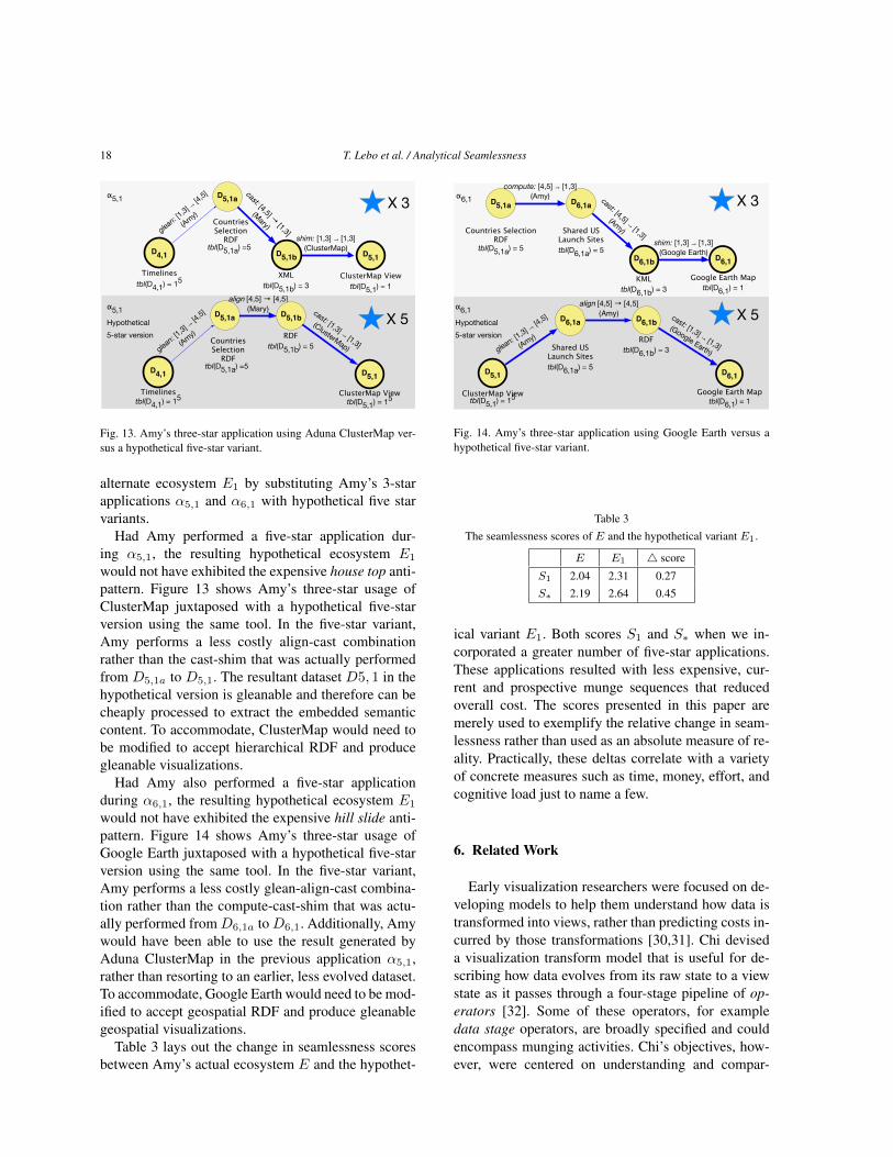
would not have exhibited the expensive hill slide anti-pattern. Figure 14 shows Amy’s three-star usage ofGoogle Earth juxtaposed with a hypothetical five-starversion using the same tool. In the five-star variant,Amy performs a less costly glean-align-cast combina-tion rather than the compute-cast-shim that was actu-ally performed fromD6,1a toD6,1. Additionally, Amywould have been able to use the result generated byAduna ClusterMap in the previous application α5,1,rather than resorting to an earlier, less evolved dataset.To accommodate, Google Earth would need to be mod-ified to accept geospatial RDF and produce gleanablegeospatial visualizations.

Table 3 lays out the change in seamlessness scoresbetween Amy’s actual ecosystem E and the hypothet-


cast: [4,5] → [1,3]

(Amy)

α6,1 D5,1a

tbl(D5,1a) = 5

Countries SelectionRDF

D6,1b

tbl(D6,1b) = 3KML

D6,1


D6,1a

tbl(D6,1a) = 5


compute: [4,5] → [1,3](Amy)

cast: [1,3] → [1,3]

(Google Earth)

α6,1Hypothetical5-star version

D6,1b

tbl(D6,1b) = 3RDF

D6,1


D6,1a

tbl(D6,1a) = 5


glean: [1,3] → [4,5]

(Amy)


D5,1

align [4,5] → [4,5](Amy)

X 3

X 5

Fig. 14. Amy’s three-star application using Google Earth versus ahypothetical five-star variant.

Table 3The seamlessness scores of E and the hypothetical variant E1.

E E1 4 score

S1 2.04 2.31 0.27S∗ 2.19 2.64 0.45

ical variant E1. Both scores S1 and S∗ when we in-corporated a greater number of five-star applications.These applications resulted with less expensive, cur-rent and prospective munge sequences that reducedoverall cost. The scores presented in this paper aremerely used to exemplify the relative change in seam-lessness rather than used as an absolute measure of re-ality. Practically, these deltas correlate with a varietyof concrete measures such as time, money, effort, andcognitive load just to name a few.

6. Related Work

Early visualization researchers were focused on de-veloping models to help them understand how data istransformed into views, rather than predicting costs in-curred by those transformations [30,31]. Chi deviseda visualization transform model that is useful for de-scribing how data evolves from its raw state to a viewstate as it passes through a four-stage pipeline of op-erators [32]. Some of these operators, for exampledata stage operators, are broadly specified and couldencompass munging activities. Chi’s objectives, how-ever, were centered on understanding and compar-


ing different visualization techniques in terms of theirpipeline structure, not their imposed costs [33].

In parallel, the visual analytics community has con-tinually developed and revised analytical cost mod-els for decades [34,35]. These models mainly considercognitive costs incurred by performing user interac-tions [36] and visual pattern recognition. In particular,Patterson presents a cognitive model of how analystsinterpret and reason with visual stimuli in order to gen-erate responses, e.g., decisions. He presents six lever-age points that visual designers should employ in or-der to reduce the costs imposed on analysts when in-terpreting visualizations [19].

When analytics researchers do consider lower leveltransforms, the result has been models that are spec-ified at too high a level to easily calculate quan-tifiable cost predictions. Wijk proposed an economicmodel that considers the ratio of value (i.e., knowledgegained) to the cost incurred to generate a visualization[37]. Wijk specifically highlighted the cost to initializedata, which can be equated to the cost of performingmunging. It is not clear, however, which specific fac-tors influence this cost, leaving analysts with little di-rection as to how to better quantify and mitigate thosecosts.

In contrast, Kandel’s work provides a more detaileddescription about the different kinds of data munginganalysts must perform and even outlines a set of re-search goals [6] that paved the way for a munging tool[23]. His hierarchy of munging types and research di-rections were elicited from actual enterprise analysts[9], the testimonies of which prove substantiating ev-idence that supports our simple theory of analyticalseamlessness. Kandel begins to discuss the use of se-mantic data types to address the challenges of format-ting, extracting, and converting data to fit input data re-quirements. He mentions that these data types shouldbe shared and reused across analyses, similar to howthe Linked Data community advocates the reuse ofpopular vocabularies [38]. However, we believe ourseamlessness theory represents the next logical step ofhis work by articulating his analysts’ testimonies in aform that can emit testable predictions.

Fink also outlined a set of challenges that wereelicited from analysts in cyber-security settings [22].He found that, like Kandel’s enterprise subjects, ana-lysts are limited by their capability to cheaply mitigatedisparities among diverse data and tools. Some of theanalysts interviewed by Fink believe that analytic en-vironments should be as flexible as UNIX shells and

allow arbitrary visualization tools to be piped together(e.g., application chains).

Meanwhile, the Linked Data community has longconsidered the potential costs and benefits associatedwith publishing and consuming linked structured data.Tim Berners-Lee is a proponent of Linked Data be-cause of the potential benefits afforded to data con-sumers, whom can more easily discover, integrate, andreuse distributed RDF 24. His scheme has been usefulin understanding the affordances provided to data con-sumers in a client-server setting, where data is onlygenerated by publishers. Our work, however, uses hisscheme to understand the costs and benefits in a peer-to-peer setting, where consumers are also publishersthat transform existing linked-data into new, additionalRDF that can be ingested by other analysts.

Similarly, Janowicz and Hitzler [39] describe howthe Semantic Web provides analysts with an opportu-nity to use third-party data in contexts not envisionedby the data provider. Analysts are able to quickly de-velop application-driven schema knowledge that canbe used to align data into arbitrary, suitable forms re-quired by tools. In the same spirit, Heath and Bizer de-scribe an application architecture for linked data ap-plications, citing data access (e.g., HTTP Get) and vo-cabulary mapping (i.e., a kind of munging) as majorcomponents [1]. The Data Integration layer that en-compasses alignment-type munges is essential for sup-porting the more abstract and user-driven applicationlayer.

When “cost” is mentioned in Linked Data literature,it is referred to in an abstract manner and not usuallyexpressed in mathematical forms from which it can becalculated. The pieces of a theory are there, howeverthey are not consolidated and formally articulated intoa framework that can be used to test and predict thecommunity’s hypotheses regarding “ease-of-use”. Webelieve our work embodies the community’s assump-tions, claims, and hypothesis as a simple theory thatcan be used to assess, predict, and refute the tenetsof Linked Data that have been advertised for nearly adecade.

7. Future Work

Our future work can be grouped into three broadsections: refining our Theory of Seamless Analytics,

24http://5stardata.info

http://5stardata.info


developing practical techniques for supporting seam-lessness, and mapping out the Linked Data landscape.Our Theory of Analytical Seamlessness can be seenas a class, where the specific set of munge activities,seamlessness metric, and application ratings can col-lectively be seen as an instance of the theory. It maybe possible to instantiate a Theory of Seamlessnessusing other factors such as cognitive load and coher-ence, so long as the instantiation is able to predict thecost to perform an analysis. The rest of this sectiondescribes future work of our specific theory instanceand therefore includes alternative munge cost order-ings and value bindings.

In terms of theory refinement, we can defer to orga-nizations and communities to help us gather evidencethat either supports or refutes our seamlessness the-ory. We would need to maintain a library of applicationchains that describe actual, realistic, and hypotheticaluses cases. Similarly to VAST challenges [40], we canask the Visual Analytics and Linked Data communitiesto implement the use cases using a variety of alternatetechnologies that challenge both the completeness andordering of our munge ontology. When our theory failsto accurately predict seamlessness, we can accommo-date by revising the membership and orderings of ourmunge hierarchy. Such an open testing framework al-lows the two communities to join forces and exposedominant cost factors using a common set of scenarios.

We can also elaborate on the distinction betweenmundane (1-3) and semantic (4-5) munges. Currently,our model stereotypes four- and five-star data into thesame class, however, we observe significant cost dif-ferences in creating five-star data. Analysts must haveexperience in good URI design, popular vocabularies25 and popular data repositories such as DBPedia 26

and datahub.io 27. Additionally, analysts need to havesome grasp of RDF patterns, such as PROV qualifiedassociations and Semantic Science Integrated Ontol-ogy (SIO) 28, so they can understand how to more ef-fectively anchor their RDF to existing linked data inmore discoverable and recognizable ways. Consider-ing this required experience, our theory should be ex-tended to account specifically for the cost of generat-ing high quality linked data. These extensions should

25Linked Open Vocabularies (LOV) maintains a listing of crowdsourced vocabularies http://lov.okfn.org/dataset/lov/

26http://dbpedia.org27http://datahub.io/28http://semanticscience.org/

draw strength from the ongoing work in the area ofLinked Data quality, while at the same time inform fu-ture work in that area.

We can also strengthen our theory by consideringthe full space of cost bindings, which may be informedby an analyst’s operational environment. Whereas thecost bindings presented in this paper are used only toexemplify relative cost savings, we expect that differ-ent organizations will specify cost bindings that betterreflect their work environment, such as the maturity oftheir staff, their familiarity with different data formats,and the size of their software toolset. For example, anorganization with a strong workforce of linked data re-searchers might further widen the cost between shim-ming and aligning to better emphasize the work force’sefficiency with semantic technologies.

Along the same line, we can update our pot func-tion to return the actual cost savings associated withsubsequent usage of results. Our current function onlyreturns a hard-coded, predicted discount based on se-mantic level of the data generated by applications. Wecan update the function to “follow up” on the actualgains by drawing from the provenance of downstreamusage [41], providing analysts with additional feed-back regarding their impact.

In terms of practical development, we can exploredifferent representations for expressing a tool’s inputssemantics. In addition to OWL, input semantics maybe represented using SPARQL and even Java inter-faces, provided the analyst’s environment is supportedby toolbox of Java APIs. An architecture that permitseither representation will allow us to concretely com-pare among associated costs, eventually converging onthe lowest cost option. We are currently developing anAPI that allows visualization widgets to self-describetheir input semantics using either representation, pro-viding us with the testing framework needed to makethe best determination. Our hopes is to invert the cur-rent asymmetry; instead of analysts spending the ma-jority of their time preparing views, we would ratherthey spend their time observing and vetting an abun-dance of automatically-generated visualization options– determined by matching data with the input seman-tics of a tool. We want to put the analyst into a “visual-ization zombie apocalypse” and change the paradigmto focus on eliminating visualizations that are not de-sirable from the abundance of what can be instantlyavailable.

Analysts could also benefit if tools were associatedwith “output” and “parameter” semantics. Althoughinput semantics help analysts get data into a tool, they



http://dbpedia.org

http://datahub.io/

http://semanticscience.org/


do not help analysts understand the products generatedby the tool. Additionally, input semantics do not helpanalysts understand how to tool can be configured tofine tune a result. Modeling the output and parametersemantics – not just the input semantics – could pro-vide a useful information to determine whether or notsuch a tool should be used, beyond whether or not itcould be used. Parameter semantics could provide use-ful information about the configuration of possible re-sults, for example, orientation, coloring, and grouping.

There is also a need for clearly-defined and moti-vated knowledge-based software development method-ologies that can help guide visualization tool devel-opers. These new development methods would rec-oncile paradigms from both the software engineeringand Linked Data communities, combining both setsof principles into a well-engineered process to buildmore seamless tools. This will allow Linked Data re-searchers to communicate the advantages of LinkedData to software engineers in the context of reducingdevelopment costs such as requirements elicitation andtesting.

When cost constrains prohibit ground-up tool devel-opment, techniques for enabling Linked Data to workwith legacy systems is also desirable. These legacysystems can exist anywhere on the spectrum from be-ing developed in-house with a white-box knowledge oftheir inner-workings, to an open source version withlimited knowledge of their inner-workings, to a fullblack box system such as Google Earth. To accom-modate, we have begun developing a method for in-telligently casting linked data to mundane represen-tations required by legacy systems while at the sametime providing the capability to return to semantic lev-els via cheap “gleans,” both from concrete representa-tions (i.e., a file) and their references (i.e. URIs).

We also need to culminate the expansive work onontology mapping to firmly establish “alignments” asa truly cheaper alternative to shimming. The mappingsolution space is large and finding the appropriate cor-respondences depends on the context of an analyst’stask. We might therefore leverage the views generatedby tools as targets that help guide analysts to the mostbeneficial mapping. As an analyst specifies a mappingand integrates data into a tool, they can inspect the vi-sual generated by the tool and judge the usefulness ofthe mapping based on the utility of the visualization.

Another novel approach to the mapping challengeis to leverage cumulative social usage history. Ratherthan using mapping ontologies as “one-off” ephemeralbridges between data and tools, the resultant ontolo-

gies could have a more global effect on reducingmunge costs of subsequent analyses. Mapping ontolo-gies should be regarded as analytical products, andused by subsequent analysts as road maps for how toalign their specific data.

In terms of the Linked Open Data cloud, we couldsupport a new era of “massive ontology landscapes”laid out from the ground-up when analysts performalignments. Considering the pairing of tools and inputsemantics, every time a new view enters an ecosys-tem its input semantics can be reconciled with allexisting input semantics, either directly or indirectlythrough property chaining. Doing so allows us toevolve broader and deeper expression of visualizationinput semantics that currently only exists implicitlywith visualization expert’s tacit knowledge based onexperience. Rather than a few organizations develop-ing monolithic ontologies describing the linked datacloud, visualization tools that publish input semanticscreate a compelling reason for analysts to build thesemapping ontologies from the ground up. The central-ized effort of developing ontologies can now be crowdsourced to analysts who are just doing their job.

8. Conclusion

We forged a Theory of Seamless Analytics that pre-dicts the cost analysts expend when performing non-trivial analyses that span across multiple applications.The theory attributes these global analytical costs tothe underlying low-level munges that transform datainto alternate representations required by tools. It sug-gests that analysts can more efficiently generate anduse materials during analyses when they perform ap-plications that require “semantic munging.”

To describe our theory, we presented an extensionof the W3C PROV Ontology that models analytic ap-plications regardless of the type of data, tool, or ob-jective involved. Our Application Ontology outlinesthree broad classes of munging that are distinguishedby the five-star rating of the data from which they oper-ate: mundane or semantic. If an analytical trace is de-scribed using our ontology, we can assess its seamless-ness by applying a metric which rewards applicationsthat process semantic data.

Our theory also describes how a particular mungesequence can be inferred from the structure of data andbehavior of tools used to perform an application. Fromthe combinations of possible data and tool behavior,we identify five configurations that are well differen-


tiated in terms of their associated munging and ratethese configurations according to their predicted cost.The pinnacle “five-star application” uses a tool’s in-put semantics and processes semantic data that leadsto cheaper munge sequences. We demonstrate this as-sociation by comparing the seamlessness of a controlanalysis centered on understanding the environmen-tal condition of Earth’s orbit with an alternate ver-sion that employs five-star applications. We observedthat the alternate version resulted with greater seman-tic munges that reduced the overall cost to perform theanalysis.

References

[1] Tom Heath and Christian Bizer. Linked data: Evolving the webinto a global data space. Synthesis lectures on the semanticweb: theory and technology, 1(1):1–136, 2011.

[2] Max Schmachtenberg, Christian Bizer, and Heiko Paulheim.Adoption of the linked data best practices in different topicaldomains. In The Semantic Web–ISWC 2014, pages 245–260.Springer, 2014.

[3] James J Thomas and Kristin A Cook. Illuminating the path:The research and development agenda for visual analytics.IEEE Computer Society Press, 2005.

[4] Shixia Liu, Weiwei Cui, Yingcai Wu, and Mengchen Liu. Asurvey on information visualization: recent advances and chal-lenges. The Visual Computer, pages 1–21, 2014.

[5] Michael Bostock, Vadim Ogievetsky, and Jeffrey Heer. D3

data-driven documents. Visualization and Computer Graphics,IEEE Transactions on, 17(12):2301–2309, 2011.

[6] Sean Kandel, Jeffrey Heer, Catherine Plaisant, Jessie Kennedy,Frank van Ham, Nathalie Henry Riche, Chris Weaver, Bong-shin Lee, Dominique Brodbeck, and Paolo Buono. Researchdirections in data wrangling: Visualizations and transforma-tions for usable and credible data. Information Visualization,10(4):271–288, 2011.

[7] Ghislain Auguste Atemezing and Raphael Troncy. TowardsInteroperable Visualization Applications Over Linked Data. InTalk Given at the 2nd European Data Forum (EDF), Dublin,Ireland (April 2013), http://goo. gl/JhVrax.

[8] Timothy Lebo, Satya Sahoo, Deborah McGuinness, KhalidBelhajjame, James Cheney, David Corsar, Daniel Garijo, StianSoiland-Reyes, Stephan Zednik, and Jun Zhao. Prov-o: Theprov ontology. W3C Recommendation, 30th April, 2013.

[9] Sean Kandel, Andreas Paepcke, Joseph M Hellerstein, and Jef-frey Heer. Enterprise data analysis and visualization: An in-terview study. Visualization and Computer Graphics, IEEETransactions on, 18(12):2917–2926, 2012.

[10] Timothy Lebo and Gregory Todd Williams. Converting gov-ernmental datasets into linked data. In Proceedings of the 6thInternational Conference on Semantic Systems, page 38. ACM,2010.

[11] LOD2 Collaborative Project. Report on Knowledge Extractionfrom Structured Sources. Technical report, 2010.

[12] RaphaÃnl Troncy Gabriel Kepeklian and Laurent Bihanic.Datalift: A platform for integrating big and linked data. In In

International Conference on Big Data from Space (BIDS’14),Rome, Italy, November 12-14, 2014 (to appear), 2014.

[13] Natalya F Noy. Semantic integration: a survey of ontology-based approaches. ACM Sigmod Record, 33(4):65–70, 2004.

[14] Carlos Buil-Aranda, Aidan Hogan, Jürgen Umbrich, andPierre-Yves Vandenbussche. SPARQL Web-Querying Infras-tructure: Ready for Action? In The Semantic Web–ISWC 2013.2013.

[15] John R Anderson. Act: Asimple theory of ecoplex cognition.American Psychologist, 51(5):355, 1996.

[16] Manolis Savva, Nicholas Kong, Arti Chhajta, Li Fei-Fei, Ma-neesh Agrawala, and Jeffrey Heer. Revision: Automated classi-fication, analysis and redesign of chart images. In Proceedingsof the 24th annual ACM symposium on User interface softwareand technology, pages 393–402. ACM, 2011.

[17] Ian Jacobs and Norman Walsh. Architecture of the world wideweb. 2004.

[18] Martin G Skjæveland. Sgvizler: A javascript wrapper for easyvisualization of sparql result sets. In Extended Semantic WebConference, 2012.

[19] Robert E Patterson, Leslie M Blaha, Georges G Grinstein,Kristen K Liggett, David E Kaveney, Kathleen C Sheldon,Paul R Havig, and Jason A Moore. A human cognition frame-work for information visualization. Computers & Graphics,42:42–58, 2014.

[20] Timothy Lebo, Alvaro Graves, and Deborah L McGuinness.Content-preserving graphics. In COLD, 2013.

[21] Marti A Hearst. User interfaces and visualization. Moderninformation retrieval, pages 257–323, 1999.

[22] Glenn A Fink, Christopher L North, Alex Endert, and StuartRose. Visualizing cyber security: Usable workspaces. In Vi-sualization for Cyber Security, 2009. VizSec 2009. 6th Interna-tional Workshop on, pages 45–56. IEEE, 2009.

[23] Sean Kandel, Andreas Paepcke, Joseph Hellerstein, and JeffreyHeer. Wrangler: Interactive visual specification of data trans-formation scripts. In Proceedings of the SIGCHI Conferenceon Human Factors in Computing Systems, pages 3363–3372.ACM, 2011.

[24] Tim Berners-Lee, James Hollenbach, Kanghao Lu, Joe Pres-brey, and Mc Schraefel. Tabulator redux: Browsing and writinglinked data. 2008.

[25] Jans Aasman and Ken Cheetham. Rdf browser for data discov-ery and visual query building. In Proceedings of the Workshopon Visual Interfaces to the Social and Semantic Web (VISSW2011), Co-located with ACM IUI, page 53, 2011.

[26] Tuukka Hastrup, Richard Cyganiak, and Uldis Bojars. Brows-ing linked data with fenfire. 2008.

[27] Mark D Wilkinson, Luke McCarthy, Benjamin Vandervalk,David Withers, Edward Kawas, and Soroush Samadian. Sadi,share, and the in silico scientific mehtod. BMC bioinformatics,11:S7, 2010.

[28] Aidan Hogan and Jü Umbrich. An empirical survey of linkeddata conformance.

[29] Marko A Rodriguez. A graph analysis of the linked data cloud.arXiv preprint arXiv:0903.0194, 2009.

[30] Stuart K Card, Jock D Mackinlay, and Ben Shneiderman.Readings in information visualization: using vision to think.Morgan Kaufmann, 1999.

[31] Robert B Haber and David A McNabb. Visualization idioms:A conceptual model for scientific visualization systems. Visu-alization in scientific computing, 74:93, 1990.


[32] Ed Huai-hsin Chi and John T Riedl. An operator interactionframework for visualization systems. In Information Visual-ization, 1998. Proceedings. IEEE Symposium on, pages 63–70.IEEE, 1998.

[33] Ed H Chi. A taxonomy of visualization techniques using thedata state reference model. In Information Visualization, 2000.InfoVis 2000. IEEE Symposium on, pages 69–75. IEEE, 2000.

[34] Daniel M Russell, Mark J Stefik, Peter Pirolli, and Stuart KCard. The cost structure of sensemaking. In Proceedings ofthe INTERACT’93 and CHI’93 conference on Human factorsin computing systems, pages 269–276. ACM, 1993.

[35] Peter Pirolli and Stuart Card. The sensemaking process andleverage points for analyst technology as identified throughcognitive task analysis. In Proceedings of International Con-ference on Intelligence Analysis, volume 5, pages 2–4. MitreMcLean, VA, 2005.

[36] Heidi Lam. A framework of interaction costs in informationvisualization. Visualization and Computer Graphics, IEEETransactions on, 14(6):1149–1156, 2008.

[37] Jarke J Van Wijk. The value of visualization. In Visualization,2005. VIS 05. IEEE, pages 79–86. IEEE, 2005.

[38] Max Schmachtenberg, Christian Bizer, and Heiko Paulheim.Adoption of the linked data bset practices in different topicaldomains. In The Semantic Web–ISWC 2014, pages 245–260.Springer, 2014.

[39] Krzysztof Janowicz and Pascal Hitzler. The digital earth asknowledge engine. Semantic Web, 2012.

[40] Kristin Cook, Georges Grinstein, Mark Whiting, MichaelCooper, Paul Havig, Kristen Liggett, Bohdan Nebesh, and Ce-leste Lyn Paul. Vast challenge 2012: Visual analytics for bigdata. In Visual Analytics Science and Technology (VAST), 2012IEEE Conference on, pages 251–255. IEEE, 2012.

[41] Timothy Lebo, Patrick West, and Deborah L. McGuinness.Walking into the future with prov pingback: An applicationto opendap using prizms (in press). In Bertram Ludaescherand Beth Plale, editors, Provenance and Annotation of Dataand Processes, Lecture Notes in Computer Science. SpringerBerlin Heidelberg, 2014.

A Five-Star Rating Scheme to Assess Application Seamlessness › system › files › swj951.pdf ·...

Documents

Transcript of A Five-Star Rating Scheme to Assess Application Seamlessness › system › files › swj951.pdf ·...