A First Look at Cellular Machine-to-Machine Traffic –Large Scale Measurement and Characterization

M. Zubair Shafiq† Lusheng Ji‡ Alex X. Liu† Jeffrey Pang‡ Jia Wang‡†Department of Computer Science and Engineering, Michigan State University, East Lansing, MI, USA

‡AT&T Labs – Research, Florham Park, NJ, USA{shafiqmu,alexliu}@cse.msu.edu, {lji,jeffpang,jiawang}@research.att.com

ABSTRACTCellular network based Machine-to-Machine (M2M) commu-nication is fast becoming a market-changing force for a widespectrum of businesses and applications such as telematics,smart metering, point-of-sale terminals, and home securityand automation systems. In this paper, we aim to answerthe following important question: Does traffic generated byM2M devices impose new requirements and challenges forcellular network design and management? To answer thisquestion, we take a first look at the characteristics of M2Mtraffic and compare it with traditional smartphone traffic.We have conducted our measurement analysis using a week-long traffic trace collected from a tier-1 cellular network inthe United States. We characterize M2M traffic from a widerange of perspectives, including temporal dynamics, devicemobility, application usage, and network performance. Ourexperimental results show that M2M traffic exhibits signifi-cantly different patterns than smartphone traffic in multipleaspects. For instance, M2M devices have a much larger ratioof uplink to downlink traffic volume, their traffic typicallyexhibits different diurnal patterns, they are more likely togenerate synchronized traffic resulting in bursty aggregatetraffic volumes, and are less mobile compared to smart-phones. On the other hand, we also find that M2M devicesare generally competing with smartphones for network re-sources in co-located geographical regions. These and otherfindings suggest that better protocol design, more carefulspectrum allocation, and modified pricing schemes may beneeded to accommodate the rise of M2M devices.

Categories and Subject DescriptorsC.2.3 [Computer System Organization]: Computer Com-munication Networks—Network Operations

KeywordsCellular Network, M2M, Mobility, Network Performance

Permission to make digital or hard copies of all or part of this work forpersonal or classroom use is granted without fee provided that copies arenot made or distributed for profit or commercial advantage and that copiesbear this notice and the full citation on the first page. To copy otherwise, torepublish, to post on servers or to redistribute to lists, requires prior specificpermission and/or a fee.SIGMETRICS’12, June 11–15, 2012, London, England, UK.Copyright 2012 ACM 978-1-4503-1097-0/12/06 ...$10.00.

1. INTRODUCTIONSmart devices that function without direct human inter-

vention are rapidly becoming an integral part of our lives.Such devices are increasingly used in applications such astelehealth, shipping and logistics, utility and environmen-tal monitoring, industrial automation, and asset tracking.Compared to traditional automation technologies, one ma-jor difference for this new generation of smart devices is howtightly they are coupled into larger scale service infrastruc-tures. For example, in logistic operations, the locations offleet vehicles can be tracked with Automatic Vehicle Loca-tion (AVL) devices such as the CalAmp LMU-2600 [7] anduploaded into back-end automatic dispatching and planningsystems for real-time global fleet management. More andmore emerging technologies also heavily depend on thesesmart devices. For instance, a corner stone for the SmartGrid Initiative is the capability of receiving and control-ling individual customer’s power usage on a real-time andwide-area basis through devices such as the electric metersequipped with Trilliant CellReader [21] modules.

This kind of leap in technology would not be possible with-out the support of wide area wireless communication infras-tructure, in particular cellular data networks. It is estimatedthat there are already tens of millions of such smart devicesconnected to cellular networks world wide and within thenext 3-5 years this number will grow to hundreds of mil-lions [3, 4]. This represents a substantial growth opportu-nity for cellular operators as mobile phone penetration rateincrease is flattening in the developed world [10,23].

M2M devices and smartphones share the same networkinfrastructure, but current cellular data networks are pri-marily designed, engineered, and managed for smartphoneusage. Given that the population of cellular M2M devicesmay soon eclipse that of smartphones, a logical question toask is: What are the challenges cellular network operatorsmay face in trying to accommodate traffic from both smart-phones and M2M devices? Existing configurations may notbe optimized to support M2M devices. In addition, M2Mdevices may compete with smartphones and impose new de-mand on shared resources. Hence, to answer this question,it is crucial to understand the M2M traffic patterns and howthey are different from traditional smartphone traffic. Theknowledge of traffic patterns can reveal insights for bettermanagement of shared network resources and ensuring bestservice quality for both types of devices.

In this paper, we take a first look at M2M traffic on acommercial cellular network. Our goal is to understand thecharacteristics of M2M traffic, in particular, whether and

how they differ from those of smartphones. To the best ofour knowledge, our study is the first to investigate the char-acteristics of traffic generated by M2M devices. We summa-rize our key contributions below.• Large Scale Measurement: We conduct the first largescale measurement study of cellular M2M traffic. For ourstudy, we have collected anonymized IP-level traffic tracesfrom the core network of a tier-1 cellular network in theUnited States. This trace covers all states in the UnitedStates during one week in August 2010. This trace containsM2M traffic from millions of devices belonging to more than150 hardware models. In addition, we have also collectedanonymized traffic traces from millions of smartphones fromthe same cellular network. Overall, we find that M2M de-vices generate significantly less traffic compared to smart-phones. Furthermore, in our trace, we observe that thenumber of M2M devices is also significantly smaller than thenumber of smartphones. However, the number of new M2Mdevices and their total traffic volume is increasing at a veryrapid pace. In fact, a longitudinal comparison of M2M trafficin this cellular network showed that total M2M traffic vol-ume has increased more than 250% in 2011. In comparison,Cisco reported that mobile data traffic grew only 132% in2011, which is almost half of the increase observed for M2Mtraffic [5]. Consequently, it is important to understand thepeculiarities of M2M traffic, especially its contrast to the tra-ditional smartphone traffic, for future network engineering.In this study, we compare M2M and smartphone traffic inthe following aspects: aggregate volume, volume time series,sessions, mobility, applications, and network performance.• Aggregate Traffic Volume: We jointly study the distri-bution of aggregate uplink and downlink traffic volume. Ourmajor finding is that, though M2M devices do not generateas much traffic as smartphones, they have a much larger ra-tio of uplink to downlink traffic volume compared to smart-phones. Since existing cellular data protocols support highercapacity in the downlink than the uplink, our finding sug-gests that network operators need careful spectrum allocationand management to avoid contention between low volume,uplink-heavy M2M traffic and high volume, downlink-heavysmartphone traffic.• Traffic Volume Time Series: We analyze the trafficvolume time series of M2M devices and smartphones. Ouranalysis shows that different M2M device models exhibit dif-ferent diurnal behaviors than smartphones. However, someM2M device models do share similar peak hours as smart-phones. Hence, M2M traffic imposes new requirements onthe shared network resources that need to be considered incapacity planning, where network is usually provisioned ac-cording to peak usage. Another finding from time series anal-ysis is that some M2M device models generate traffic in asynchronized fashion (like a botnet [20]), which can resultin denial of service due to limited radio spectrum. There-fore, M2M protocols should randomize such network usageto avoid congesting the radio network.• Traffic Sessions: To understand the usage behavior ofindividual devices, we conduct session-level traffic analysisin terms of active time, session length, and session inter-arrival time. We find that high traffic volume does not al-ways correlate with more active time. This finding callsfor new billing schemes, which go beyond per-byte chargingmodels. We also find that M2M devices have different ses-sion length and inter-arrival time characteristics compared

to smartphones. This finding can be utilized by device man-ufacturers to improve battery management and by networkoperators to optimize radio network parameters for M2M de-vices.• Device Mobility: We compare the mobility character-istics of M2M devices and smartphones from individual de-vice and network perspectives. We find that M2M devices,with a few exceptions, are less mobile than smartphones.We also find that M2M and smartphone traffic competes fornetwork resources in co-located geographical regions. Thisfinding indicates that careful network resource allocation isrequired to avoid contention between low-volume M2M trafficand high-volume smartphone traffic.• Application Usage: We also study the contribution ofdifferent applications to the aggregate traffic volume of M2Mdevices and smartphones. We find that M2M traffic mostlyuses non-standard and custom application protocols, whichis undesirable because it is difficult for network operators tounderstand and mitigate adverse effects from these protocolscompared to standard protocols.• Network Performance: The network performance re-sults of M2M traffic, in terms of packet loss ratio and roundtrip time, show strong dependency on device radio technol-ogy (2G or 3G) and expected device environment (e.g. in-doors vs. outdoors). This implies that network operatorsmust continue to support and improve legacy networks forM2M devices even as smartphones move to 4G technologies.

The rest of this paper proceeds as follows. We first pro-vide details of our collected trace in Section 2. Sections 3–8present measurement analysis of M2M traffic and comparethem to traditional smartphone traffic. Finally, we reviewthe related work in Section 9 and conclude in Section 10.

2. DATA2.1 Data Set

The data used in this study is collected from a nation-widecellular operator in the United States that provides 2G and3G cellular data services. It supports GPRS, EDGE, UMTS,and HSPA technologies. Architecturally, the portion of itsnetwork that supports cellular data service is organized intwo tiers. The lower tier, the radio access network, provideswireless connectivity to user devices, and the upper tier, thecore network, interfaces the cellular data network with theInternet. More details about cellular data network architec-ture can be found in prior literature such as [2].

The data collection apparatus that produced the traceused in our study is deployed at all links between ServingGateway Support Nodes (SGSN) and Gateway GRPS Sup-port Nodes (GGSN) in the core network. This apparatusis capable of anonymously logging session level traffic in-formation at 5 minute intervals for all IP data traffic be-tween cellular devices and the Internet. In other words,each record in the trace is a 5-minute traffic volume sum-mary aggregated by unique device identifier and applicationcategory. Each record also contains the cell location of thedevice at the start of the session. Each record is originallytimestamped according to the standard coordinated univer-sal time (UTC), which is then converted to the local timeat the device for our analysis. This trace was collected dur-ing one complete week in August 2010. Geographically, thetrace covers the whole United States. Applications are iden-tified using a combination of port information, HTTP hostand user-agent information, and other heuristics [9]. More

information about the data collection system can be foundin [9, 18].

2.2 M2M Device CategorizationThe data set contains traffic records for all cellular de-

vices, so we first need to separate M2M devices from therest. Furthermore, because M2M devices are usually devel-oped for specific applications, significant behavioral differ-ences are expected between M2M devices for different targetapplications. Thus, it is reasonable to sub-divide M2M de-vices into categories based on their intended application tobetter understand the unique traffic characteristics of dif-ferent M2M categories. We start this process by identifyingthe hardware model of each cellular device using the device’sType Allocation Code (TAC), which is part of the uniqueidentifier of each cellular device. Although the records inour data set are anonymized, the TAC portion of the uniqueID is retained. Thus, the hardware model of each cellulardevice is obtained by consulting the TAC database of theGSM Association.

Because there is no rigorous definition for M2M devices orstandard ways for determining their application categories,and many devices have multiple uses, knowing the devicemodel is not sufficient for identifying a device with certaintyas M2M device nor for identifying its M2M category. To-wards this end, we adopt the device classification scheme ofa major cellular service provider as a base template for cat-egorizing M2M devices [1]. To supplement and verify thistemplate, we also use public information such as productionbrochures and specification sheets. In total, we have clas-sified more than 150 device models as M2M devices, andfurther divide them into the following 6 categories.1) Asset Tracking: These M2M devices are used to re-motely track objects like cargo containers and other ship-ments. These devices are often coupled with other sensorsfor tasks like temperature and pressure measurement. Inour trace, about 18% devices belong to this category.2) Building Security: These M2M devices are typicallyused to manage door access and security cameras. In ourtrace, about 14% devices belong to this category.3) Fleet: These M2M devices are used to monitor vehiclelocations, arrivals, and departures and provide real-time ac-cess to critical operational data for logistic service providers.In our trace, about 51% devices belong to this category.4) Modem: These M2M devices are used as generic cellularcommunication modems with embedded system data inputand output ports such as serial, I2C, analog, and digital.They provide network connectivity for customized solutions.In our trace, about 9% devices belong to this category.5) Metering: These M2M devices are mostly used for re-mote measurement and monitoring in agricultural, environ-mental, and energy applications. In our trace, about 6%devices belong to this category.6) Telehealth: These M2M devices are mostly used forremote measurement and monitoring in healthcare applica-tions. In our trace, about 2% devices belong to this category.

We acknowledge that due to lack of more detailed usageinformation and ambiguity in device registry databases, ourclassification may contain some errors. To limit such er-rors, we try to be as conservative as possible when decidingwhether to include a M2M device model in our study. Forexample, cellular routers are generally excluded from thisstudy because the actual end devices behind these routers

1 2 3 40

0.2

0.4

0.6

0.8

1

Normalized downlink traffic volume

CD

F

SmartphoneM2MAssetBuildingFleetModemMeteringTelehealth

(a) Downlink

1 2 3 40

0.2

0.4

0.6

0.8

1

Normalized uplink traffic volume

CD

F

SmartphoneM2MAssetBuildingFleetModemMeteringTelehealth

(b) Uplink

−1 −0.8 −0.6 −0.4 −0.2 0 0.2 0.4 0.6 0.8 10

0.2

0.4

0.6

0.8

1

CD

F

Z

SmartphoneM2MAssetBuildingFleetModemMeteringTelehealth

(c) Ratio: log(Uplink/Downlink)

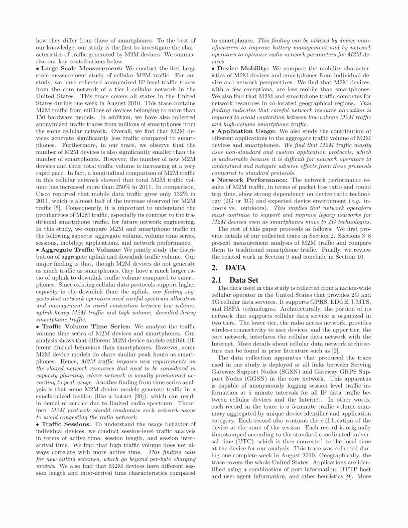
Figure 1: CDFs of aggregate downlink and uplinktraffic volume.

cannot be identified. For cellular modems and modules, weexclude models with data interfaces likely used by modernday computers such as USB, PCI Express, and miniPCI butkeep those with UART, SPI, and I2C interfaces. For thesake of comparing M2M and typical human-generated traf-fic characteristics, we have also included in our study trafficrecords from a uniformly sampled set of smartphone models,covering millions of smartphone devices.

In the following sections, based on this collected trace, weconduct a detailed analysis of M2M traffic characteristicsand compare them with those of the smartphones found inthe same trace. The traffic characteristics analyzed in thispaper include aggregate data volume, volume time series,session analysis, mobility, application usage, and networkperformance.

3. AGGREGATE TRAFFIC VOLUMEWhen a new technology emerges and it has to share re-

sources with existing parties, a natural first question is thelevel of competition and how different parties can better co-exist. This is why we first study and compare the distribu-tion of aggregate traffic volume for M2M devices and smart-phones. Moreover, we also investigate whether the long es-tablished perception of traffic volume being downlink heavyremains true for M2M devices [15].

Figure 1 shows the cumulative distribution functions(CDFs) of downlink and uplink normalized traffic volumefor M2M devices and smartphones separately. To normalizetraffic volume, we divided the maximum observed volume byan arbitrary constant. For M2M, we show both the distribu-tions for all M2M devices together and for each M2M cate-gory. We first notice that different device categories exhibit

strong diversity in aggregate downlink and uplink traffic vol-ume distributions. However, we do observe a consistent rel-ative ordering of CDFs for different device categories. Wenote that the average aggregate downlink and uplink trafficvolume for smartphones is several orders of magnitude largercompared to all M2M device categories. Within M2M devicecategories, modem category has the largest downlink trafficvolume, followed by asset category; whereas, building secu-rity and fleet categories have the smallest downlink trafficvolume. A similar ordering is also observed for uplink trafficvolume.

We now study the distribution of ratios of uplink trafficvolume to downlink traffic volume. For the sake of clar-ity, we plot the ratios after taking their logarithm, denotedby Z. The positive values of Z represent more uplink traf-fic volume than downlink traffic volume and its negativevalues represent more downlink traffic volume than uplinktraffic volume. It is not surprising that approximately 80%of smartphone devices have Z ≤ 0; thereby, indicating largerdownlink traffic volumes. However, this trend is reversed bylarge margin for all M2M device categories, which all haveZ > 0 for more than 80% of devices indicating larger uplinktraffic volumes. This finding provides another evidence thatM2M traffic has significantly different characteristics com-pared to traditional smartphone traffic. Comparing differentM2M device categories, we observe that building and me-tering categories have the lowest average Z values; whereas,asset and telehealth have the highest average Z values. Suchdifferences provide insight into the functionality of M2M de-vice categories.Summary: Overall, the average per-device traffic volumeof M2M devices is much smaller than that of smartphones.However, the strength of M2M devices is really in the sizeof their population. As M2M population continues to in-crease, how network operators efficiently support a largenumber of low volume devices will become an important is-sue. Our finding that M2M traffic has a much larger ratio ofuplink to downlink traffic volume compared to smartphonetraffic shows that M2M devices act more as “content pro-ducers” than “content consumers”, unlike traditional smart-phone devices. Interestingly, this difference coincides withthe paradigm shift in web and mobile computing towardsuser-centric content generation. The momentum of such ashift may eventually question the assumptions for optimiza-tion approaches exploiting downlink asymmetry of networktraffic [14].

4. TRAFFIC VOLUME TIME SERIESHaving gained an understanding of aggregated M2M traf-

fic volume, the next step is to study the temporal dynamicsof M2M traffic volume. It would be interesting to knowwhether M2M devices exhibit similar daily diurnal patternas smartphones. One particular use of such information isto evaluate the potential benefits of incentive programs suchas billing discounts encouraging non-peak time usage. Timeseries analysis is also helpful for gaining insights into theoperations of M2M devices.

As mentioned in Section 2, the logged traffic records con-tain timestamps at 5-minute time resolution. Therefore, wecan separately construct averaged traffic volume time seriesfor smartphones and all M2M device categories. We plotthese averaged uplink and downlink traffic volume time se-ries in Figure 2. While the daily diurnal pattern is evident

24 12 6 3 2 1 1/2 1/40

10

20

30

40

Time period (hours)

Pow

er/fr

eque

ncy

(dB

/Hz)

SmartphoneM2MModemMetering

(a) Downlink

24 12 6 3 2 1 1/2 1/40

10

20

30

40

Time period (hours)

Pow

er/fr

eque

ncy

(dB

/Hz)

SmartphoneM2MModemMetering

(b) Uplink

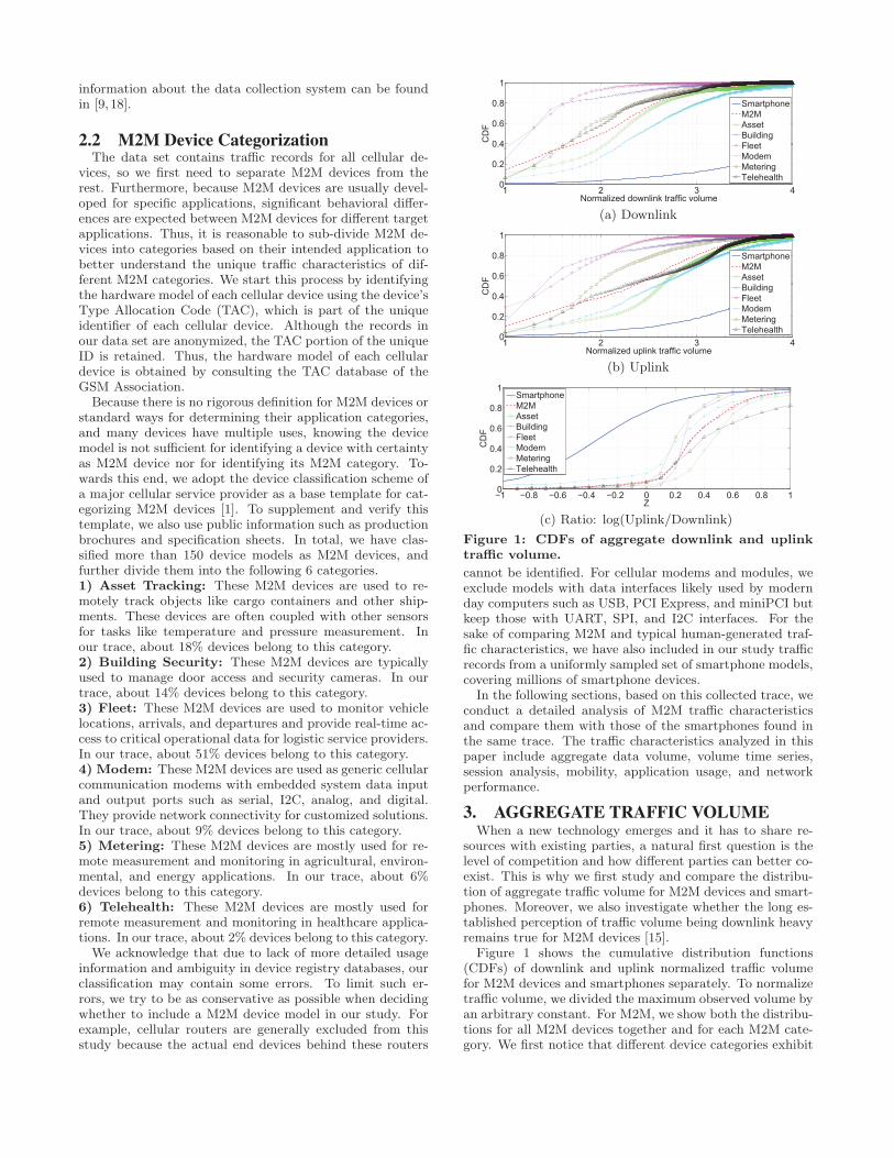
Figure 3: Periodograms containing power spectraldensity estimate of traffic volume time series.

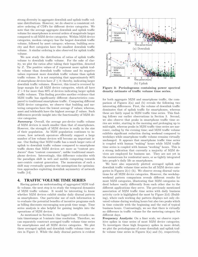
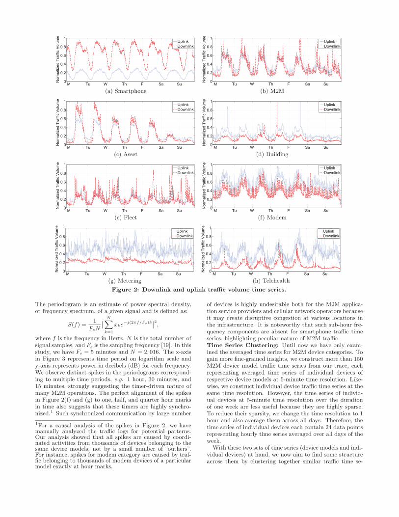
for both aggregate M2M and smartphone traffic, the com-parison of Figures 2(a) and (b) reveals the following twointeresting differences. First, the volume of downlink trafficdominates that of uplink traffic for smartphones, whereasthese are fairly equal in M2M traffic time series. This find-ing follows our earlier observations in Section 3. Second,we also observe that peaks in smartphone traffic time se-ries are wider, starting in the morning and prolonging up tomid-night, whereas peaks in M2M traffic time series are nar-rower, ending by the evening time; and M2M traffic volumeexhibits significant reduction during weekend compared toweekdays while smartphone traffic volume remains virtuallyunchanged. It appears that smartphone traffic time seriesis coupled with human “waking” hours while M2M traffictime series is coupled with human “working” hours. This isa strong indication that currently a majority of M2M de-vices are employed for business use. They are not yet inthe mainstream for residential users, or as tightly integratedinto people’s daily life as smartphones.

We have also separately plotted averaged uplink anddownlink traffic volume time series for all M2M device cate-gories in Figures 2(c)–(h). We observe strong diurnal varia-tions for all M2M device categories. However, the weekday-weekend pattern comparison reveals different results formost M2M categories, illustrating that M2M categories in-deed behave vastly differently from each other due to thedifferent applications they serve. The previously mentionedassociation of M2M traffic time series with daily businessactivity cycle is highlighted the most by Figure 2(d) (Build-ing), where each working day pattern displays not only ele-vated volume during working hours but also two peaks whichin time coincide with the beginning and the end of typicalbusiness hours. Contrastingly, we see that there is virtuallyno difference in traffic volume for the metering category fordifferent days.Frequency Analysis: On a finer scale, we observe repet-itive spikes in time series of most M2M device categories.To investigate these high frequency spikes in more detail,we plot the periodograms of some downlink and uplink traf-fic volume time series in Figures 3(a) and (b), respectively.

M Tu W Th F Sa Su0

0.2

0.4

0.6

0.8

1

Nor

mal

ized

Tra

ffic

Vol

ume

UplinkDownlink

(a) Smartphone

M Tu W Th F Sa Su0

0.2

0.4

0.6

0.8

1

Nor

mal

ized

Tra

ffic

Vol

ume

UplinkDownlink

(b) M2M

M Tu W Th F Sa Su0

0.2

0.4

0.6

0.8

1

Nor

mal

ized

Tra

ffic

Vol

ume

UplinkDownlink

(c) Asset

M Tu W Th F Sa Su0

0.2

0.4

0.6

0.8

1

Nor

mal

ized

Tra

ffic

Vol

ume

UplinkDownlink

(d) Building

M Tu W Th F Sa Su0

0.2

0.4

0.6

0.8

1

Nor

mal

ized

Tra

ffic

Vol

ume

UplinkDownlink

(e) Fleet

M Tu W Th F Sa Su0

0.2

0.4

0.6

0.8

1

Nor

mal

ized

Tra

ffic

Vol

ume

UplinkDownlink

(f) Modem

M Tu W Th F Sa Su0

0.2

0.4

0.6

0.8

1

Nor

mal

ized

Tra

ffic

Vol

ume

UplinkDownlink

(g) Metering

M Tu W Th F Sa Su0

0.2

0.4

0.6

0.8

1

Nor

mal

ized

Tra

ffic

Vol

ume

UplinkDownlink

(h) Telehealth

Figure 2: Downlink and uplink traffic volume time series.

The periodogram is an estimate of power spectral density,or frequency spectrum, of a given signal and is defined as:

S(f) =1

FsN

∣∣ N∑k=1

xke−j(2πf/Fs)k

∣∣2,where f is the frequency in Hertz, N is the total number ofsignal samples, and Fs is the sampling frequency [19]. In thisstudy, we have Fs = 5 minutes and N = 2, 016. The x-axisin Figure 3 represents time period on logarithm scale andy-axis represents power in decibels (dB) for each frequency.We observe distinct spikes in the periodograms correspond-ing to multiple time periods, e.g. 1 hour, 30 minutes, and15 minutes, strongly suggesting the timer-driven nature ofmany M2M operations. The perfect alignment of the spikesin Figure 2(f) and (g) to one, half, and quarter hour marksin time also suggests that these timers are highly synchro-nized.1 Such synchronized communication by large number

1For a causal analysis of the spikes in Figure 2, we havemanually analyzed the traffic logs for potential patterns.Our analysis showed that all spikes are caused by coordi-nated activities from thousands of devices belonging to thesame device models, not by a small number of “outliers”.For instance, spikes for modem category are caused by traf-fic belonging to thousands of modem devices of a particularmodel exactly at hour marks.

of devices is highly undesirable both for the M2M applica-tion service providers and cellular network operators becauseit may create disruptive congestion at various locations inthe infrastructure. It is noteworthy that such sub-hour fre-quency components are absent for smartphone traffic timeseries, highlighting peculiar nature of M2M traffic.Time Series Clustering: Until now we have only exam-ined the averaged time series for M2M device categories. Togain more fine-grained insights, we construct more than 150M2M device model traffic time series from our trace, eachrepresenting averaged time series of individual devices ofrespective device models at 5-minute time resolution. Like-wise, we construct individual device traffic time series at thesame time resolution. However, the time series of individ-ual devices at 5-minute time resolution over the durationof one week are less useful because they are highly sparse.To reduce their sparsity, we change the time resolution to 1hour and also average them across all days. Therefore, thetime series of individual devices each contain 24 data pointsrepresenting hourly time series averaged over all days of theweek.

With these two sets of time series (device models and indi-vidual devices) at hand, we now aim to find some structureacross them by clustering together similar traffic time se-

0

5

10

15

20

25

30

35

Dis

tanc

e

Index

(a) Device model

0

1

2

3

4

5

Dis

tanc

e

Index

(b) Individual device

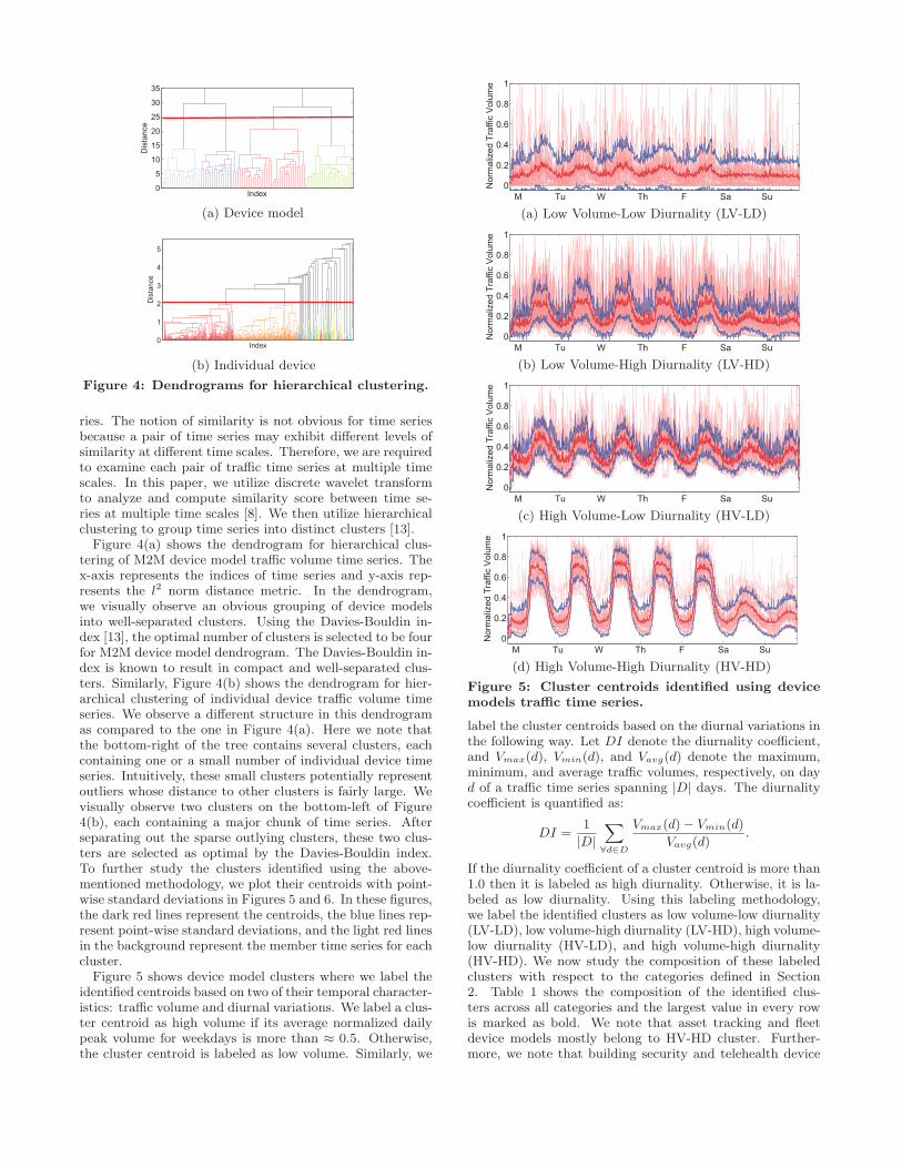
Figure 4: Dendrograms for hierarchical clustering.

ries. The notion of similarity is not obvious for time seriesbecause a pair of time series may exhibit different levels ofsimilarity at different time scales. Therefore, we are requiredto examine each pair of traffic time series at multiple timescales. In this paper, we utilize discrete wavelet transformto analyze and compute similarity score between time se-ries at multiple time scales [8]. We then utilize hierarchicalclustering to group time series into distinct clusters [13].

Figure 4(a) shows the dendrogram for hierarchical clus-tering of M2M device model traffic volume time series. Thex-axis represents the indices of time series and y-axis rep-resents the l2 norm distance metric. In the dendrogram,we visually observe an obvious grouping of device modelsinto well-separated clusters. Using the Davies-Bouldin in-dex [13], the optimal number of clusters is selected to be fourfor M2M device model dendrogram. The Davies-Bouldin in-dex is known to result in compact and well-separated clus-ters. Similarly, Figure 4(b) shows the dendrogram for hier-archical clustering of individual device traffic volume timeseries. We observe a different structure in this dendrogramas compared to the one in Figure 4(a). Here we note thatthe bottom-right of the tree contains several clusters, eachcontaining one or a small number of individual device timeseries. Intuitively, these small clusters potentially representoutliers whose distance to other clusters is fairly large. Wevisually observe two clusters on the bottom-left of Figure4(b), each containing a major chunk of time series. Afterseparating out the sparse outlying clusters, these two clus-ters are selected as optimal by the Davies-Bouldin index.To further study the clusters identified using the above-mentioned methodology, we plot their centroids with point-wise standard deviations in Figures 5 and 6. In these figures,the dark red lines represent the centroids, the blue lines rep-resent point-wise standard deviations, and the light red linesin the background represent the member time series for eachcluster.

Figure 5 shows device model clusters where we label theidentified centroids based on two of their temporal character-istics: traffic volume and diurnal variations. We label a clus-ter centroid as high volume if its average normalized dailypeak volume for weekdays is more than ≈ 0.5. Otherwise,the cluster centroid is labeled as low volume. Similarly, we

M Tu W Th F Sa Su0

0.2

0.4

0.6

0.8

1

Nor

mal

ized

Tra

ffic

Vol

ume

(a) Low Volume-Low Diurnality (LV-LD)

M Tu W Th F Sa Su0

0.2

0.4

0.6

0.8

1

Nor

mal

ized

Tra

ffic

Vol

ume

(b) Low Volume-High Diurnality (LV-HD)

M Tu W Th F Sa Su0

0.2

0.4

0.6

0.8

1

Nor

mal

ized

Tra

ffic

Vol

ume

(c) High Volume-Low Diurnality (HV-LD)

M Tu W Th F Sa Su0

0.2

0.4

0.6

0.8

1

Nor

mal

ized

Tra

ffic

Vol

ume

(d) High Volume-High Diurnality (HV-HD)

Figure 5: Cluster centroids identified using devicemodels traffic time series.

label the cluster centroids based on the diurnal variations inthe following way. Let DI denote the diurnality coefficient,and Vmax(d), Vmin(d), and Vavg(d) denote the maximum,minimum, and average traffic volumes, respectively, on dayd of a traffic time series spanning |D| days. The diurnalitycoefficient is quantified as:

DI =1

|D|∑∀d∈D

Vmax(d)− Vmin(d)

Vavg(d).

If the diurnality coefficient of a cluster centroid is more than1.0 then it is labeled as high diurnality. Otherwise, it is la-beled as low diurnality. Using this labeling methodology,we label the identified clusters as low volume-low diurnality(LV-LD), low volume-high diurnality (LV-HD), high volume-low diurnality (HV-LD), and high volume-high diurnality(HV-HD). We now study the composition of these labeledclusters with respect to the categories defined in Section2. Table 1 shows the composition of the identified clus-ters across all categories and the largest value in every rowis marked as bold. We note that asset tracking and fleetdevice models mostly belong to HV-HD cluster. Further-more, we note that building security and telehealth device

Table 1: Composition of device model clusters.LV-LD LV-HD HV-LD HV-HD

% % % %Asset 13.1 16.1 23.5 33.3

Building 13.1 19.3 11.7 0.0Fleet 26.2 29.2 5.9 61.2

Modem 34.5 25.8 47.1 5.5Metering 13.1 3.2 5.9 0.0Telehealth 0.0 6.4 5.9 0.0

models mostly belong to LV-HD cluster. These observa-tions follow our intuition that the activity of these devicemodels is tightly coupled with human activities. They alsoindicate that building security and telehealth device modelstend to generate low traffic volume. Similarly, we observethat metering device models mostly belong to LV-LD clus-ter. This observation follows our earlier finding from Figure3 that metering devices tend to download or upload dataafter periodic time intervals throughout the day. Finally, weobserve that modem device models mostly belong to HV-LDclusters. Similar to metering device models, modem devicemodels also tend to generate traffic after periodic time in-tervals throughout the day resulting in low diurnality.

For individual device traffic volume time series clustering,we identified a handful number of outlier clusters and twomain clusters containing a majority of devices. We plot thecentroids of two main clusters and one of the outlier clustersin Figure 6. The cluster centroid in Figure 6(a) shows strongdiurnal behavior with higher traffic volume during day timeas compared to night time; therefore, we label this cluster asdiurnal. On the other hand, the cluster centroid in Figure6(b) does not show any diurnal characteristics and is la-beled as flat. We also show an outlier cluster in Figure 6(c),which consists of devices generating traffic volume spikes atlate night. To gain insights from the clustering results ofindividual device traffic volume time series, we study theircomposition across various M2M device categories. Table 2shows the cluster composition results with the largest valuein every row marked as bold. We have similar observationsfor device level clustering as we previously had for devicemodel traffic volume time series clustering. For instance,asset tracking and fleet devices mostly belong to the diur-nal cluster. Modem, metering, and telehealth devices, withspiky traffic volume time series, mostly belong to the outliercluster. Finally, building security devices mostly belong tothe flat cluster. The individual device level clustering resultsfurther improve the confidence of our understanding aboutthe behavior of M2M devices.Summary: In this section, we have presented time seriesanalysis for M2M traffic volume. Just like that of smart-phones, M2M traffic volume also exhibits strong daily diur-nal pattern. However, M2M traffic volume peaks correspondto people’s working hours while smartphone traffic volumepeaks correspond to waking hours, which indicates that amajority of M2M devices are employed for business use.The overlap between M2M peaks and smartphone peakssuggests that incentive based leverage mechanism such asoff-peak time pricing for encouraging better sharing of net-work capacity can be beneficial. We have also investigatedfine-grained features in traffic volume time series for differentcategories and uncovered the differences in behaviors amongdifferent M2M categories. For example unlike other M2Mcategories, metering devices show only weak diurnal pattern,suggesting that the traditional approach of scheduling ser-

0 1 2 3 4 5 6 7 8 9 10 11 12 13 14 15 16 17 18 19 20 21 22 230

0.2

0.4

0.6

0.8

Nor

mal

ized

Tra

ffic

Vol

ume

Hour of day

(a) Diurnal

0 1 2 3 4 5 6 7 8 9 10 11 12 13 14 15 16 17 18 19 20 21 22 230

0.2

0.4

0.6

0.8

1

Nor

mal

ized

Tra

ffic

Vol

ume

Hour of day

(b) Flat

0 1 2 3 4 5 6 7 8 9 10 11 12 13 14 15 16 17 18 19 20 21 22 230

0.2

0.4

0.6

0.8

1

Nor

mal

ized

Tra

ffic

Vol

ume

Hour of day

(c) An outlier cluster

Figure 6: Cluster centroids identified using individ-ual device traffic time series.Table 2: Composition of individual device time se-ries clusters.

Diurnal Flat Outlier% % %

Asset 16.9 15.7 4.8Building 11.8 19.1 15.7Fleet 57.1 47.5 44.6

Modem 8.3 11.1 12.0Metering 2.3 3.8 9.6Telehealth 3.6 2.8 13.3

vice down time in early morning hours may not be the bestfor them. Finally, the surprising discovery of synchronizedcommunication among M2M devices highlights the impor-tance of developing and imposing standard traffic protocolsand randomization methods.

5. SESSION ANALYSISWe now analyze and compare session-level traffic charac-

teristics of M2M devices and smartphones. Understandingsession duration and inter-arrival distribution is a time hon-ored tradition for the telecommunication industry becausethey are important inputs for network resource planning andmanagement. Such information is valuable for cellular net-work operators too because device active time correspondsmore closely to radio resource usage than aggregate trafficvolume [17]. Moreover, being able to accurately estimatesession timing parameters not only improves radio resourceuse efficiency for cellular operators, it also helps M2M ser-vice providers to better design their devices and protocolsfor better battery management.

Towards this end, we first formally define a session andthen study different metrics based on session-level informa-tion. A flow consists of all packets in a given transport layer

connection, including TCP and UDP. To study character-istics of flows at a given time resolution, we need to defineequally-spaced time bins denoted by Δi where i = 1, 2, ...and |Δ| denotes the magnitude of time bin and i is the indexvariable. Recall from Section 2 that the smallest availabletime resolution in our traffic trace is 5 minutes; therefore,we use |Δ| = 5 minutes for the rest of this section. We lookat flow arrivals in 5 minute time bins as a binary randomprocess, which is denoted by {Ft : t ∈ T, F ∈ {0, 1}} andwhere 0 and 1 respectively denote absence or presence offlow arrival, respectively. We now define a session as a runof flow arrivals in consecutive time bins, where a flow span-ning multiple time bins is marked for all time bins during itsspan. A session is denoted by S{tx(i),ty(i)}, where tx(i) andty(i) are the times corresponding to the first flow arrival andthe last flow arrival of i-th session. In the following text, weseparately investigate several metrics that capture diversecharacteristics of the session arrival process.Active Time: The first metric that we study is deviceactive time, denoted by Tactive, which is the total amountof time in our week-long trace when a device has traffic. Inour study, it is calculated by multiplying number of uniquetime bins in which we have at least one flow arrival by thebin duration. Using this metric, we are primarily interestedin studying the impact of devices on the network in terms ofradio channel occupation. Note that a given time bin mayhave multiple flow arrivals but they are all mapped to 1.Mathematically, active time is defined as:

Tactive =∑∀t∈T

Ft (counts) =∑∀t∈T

Ft ∗ |Δ| (time units).

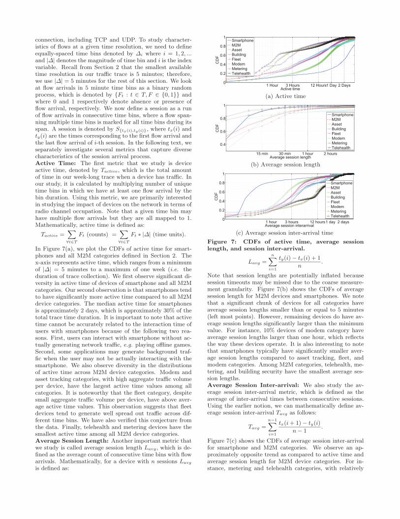
In Figure 7(a), we plot the CDFs of active time for smart-phones and all M2M categories defined in Section 2. Thex-axis represents active time, which ranges from a minimumof |Δ| = 5 minutes to a maximum of one week (i.e. theduration of trace collection). We first observe significant di-versity in active time of devices of smartphone and all M2Mcategories. Our second observation is that smartphones tendto have significantly more active time compared to all M2Mdevice categories. The median active time for smartphonesis approximately 2 days, which is approximately 30% of thetotal trace time duration. It is important to note that activetime cannot be accurately related to the interaction time ofusers with smartphones because of the following two rea-sons. First, users can interact with smartphone without ac-tually generating network traffic, e.g. playing offline games.Second, some applications may generate background traf-fic when the user may not be actually interacting with thesmartphone. We also observe diversity in the distributionsof active time across M2M device categories. Modem andasset tracking categories, with high aggregate traffic volumeper device, have the largest active time values among allcategories. It is noteworthy that the fleet category, despitesmall aggregate traffic volume per device, have above aver-age active time values. This observation suggests that fleetdevices tend to generate well spread out traffic across dif-ferent time bins. We have also verified this conjecture fromthe data. Finally, telehealth and metering devices have thesmallest active time among all M2M device categories.Average Session Length: Another important metric thatwe study is called average session length Lavg, which is de-fined as the average count of consecutive time bins with flowarrivals. Mathematically, for a device with n sessions Lavg

is defined as:

1 Hour 3 Hours 12 Hours1 Day 2 Days0

0.2

0.4

0.6

0.8

1

Active time

CD

F

SmartphoneM2MAssetBuildingFleetModemMeteringTelehealth

(a) Active time

15 min 30 min 1 hour 2 hours

0.4

0.6

0.8

1

Average session length

CD

F

SmartphoneM2MAssetBuildingFleetModemMeteringTelehealth

(b) Average session length

1 hour 3 hours 12 hours1 day 2 days0

0.2

0.4

0.6

0.8

1

Average session interarrival

CD

F

SmartphoneM2MAssetBuildingFleetModemMeteringTelehealth

(c) Average session inter-arrival time

Figure 7: CDFs of active time, average sessionlength, and session inter-arrival.

Lavg =n∑

i=1

ty(i)− tx(i) + 1

n.

Note that session lengths are potentially inflated becausesession timeouts may be missed due to the coarse measure-ment granularity. Figure 7(b) shows the CDFs of averagesession length for M2M devices and smartphones. We notethat a significant chunk of devices for all categories haveaverage session lengths smaller than or equal to 5 minutes(left most points). However, remaining devices do have av-erage session lengths significantly larger than the minimumvalue. For instance, 10% devices of modem category haveaverage session lengths larger than one hour, which reflectsthe way these devices operate. It is also interesting to notethat smartphones typically have significantly smaller aver-age session lengths compared to asset tracking, fleet, andmodem categories. Among M2M categories, telehealth, me-tering, and building security have the smallest average ses-sion lengths.Average Session Inter-arrival: We also study the av-erage session inter-arrival metric, which is defined as theaverage of inter-arrival times between consecutive sessions.Using the earlier notion, we can mathematically define av-erage session inter-arrival Tavg as follows:

Tavg =

n−1∑i=1

tx(i+ 1)− ty(i)

n− 1.

Figure 7(c) shows the CDFs of average session inter-arrivalfor smartphone and M2M categories. We observe an ap-proximately opposite trend as compared to active time andaverage session length for M2M device categories. For in-stance, metering and telehealth categories, with relatively

small active time and average session lengths, have relativelylarge average session inter-arrival time with median valuesof approximately 9 hours. On the other hand, asset trackingand fleet categories have relatively relatively small averagesession inter-arrival time with median values of less than 3hours. Smartphones tend to have even smaller average ses-sion inter-arrival time, where approximately 80% of deviceshave less than one hour average session inter-arrival time.Summary: Once again, M2M traffic sessions exhibit ratherdifferent characteristics from smartphone traffic sessions.Overall M2M devices are active for traffic for much less timethan smartphones. M2M traffic sessions occur much less fre-quently. It is especially worth noting that 3 out of 6 M2Mcategories have about 80% of the devices with average ses-sion time lasting less than 5 minutes. This indicates thatbyte volume of data traffic for these devices is likely not anaccurate reflection of their network resource use due to dis-proportional amount of control plane overhead for establish-ing and tearing down short sessions. The large differencesbetween different M2M categories also advocate for differ-entiated radio resource control configurations for differentcategories.

6. MOBILITYIn this section, we study and compare the mobility charac-

teristics and geographical distribution of M2M devices andsmartphones. Mobility patterns for different devices, con-structed from our nation-wide trace, helps establishing anunderstanding for how much they move. Understanding mo-bility patterns for different devices has a direct impact onnetwork resource planning. More importantly, we are in-terested in investigating how the locations of M2M devicepopulation are distributed relative to those of smartphones.Previously in Section 4, we have discovered that M2M traf-fic volume peaks overlap with those of smartphones in time.Here we investigate whether they also overlap in space.

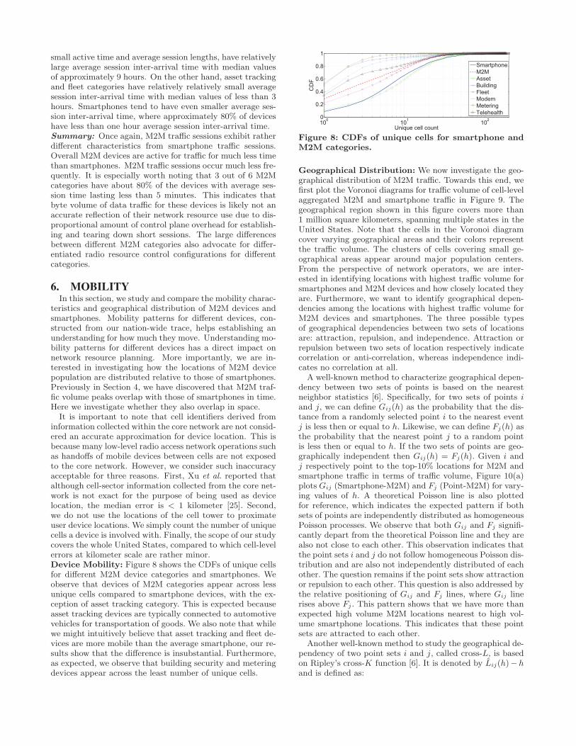
It is important to note that cell identifiers derived frominformation collected within the core network are not consid-ered an accurate approximation for device location. This isbecause many low-level radio access network operations suchas handoffs of mobile devices between cells are not exposedto the core network. However, we consider such inaccuracyacceptable for three reasons. First, Xu et al. reported thatalthough cell-sector information collected from the core net-work is not exact for the purpose of being used as devicelocation, the median error is < 1 kilometer [25]. Second,we do not use the locations of the cell tower to proximateuser device locations. We simply count the number of uniquecells a device is involved with. Finally, the scope of our studycovers the whole United States, compared to which cell-levelerrors at kilometer scale are rather minor.Device Mobility: Figure 8 shows the CDFs of unique cellsfor different M2M device categories and smartphones. Weobserve that devices of M2M categories appear across lessunique cells compared to smartphone devices, with the ex-ception of asset tracking category. This is expected becauseasset tracking devices are typically connected to automotivevehicles for transportation of goods. We also note that whilewe might intuitively believe that asset tracking and fleet de-vices are more mobile than the average smartphone, our re-sults show that the difference is insubstantial. Furthermore,as expected, we observe that building security and meteringdevices appear across the least number of unique cells.

100 101 1020

0.2

0.4

0.6

0.8

1

Unique cell count

CD

F

SmartphoneM2MAssetBuildingFleetModemMeteringTelehealth

Figure 8: CDFs of unique cells for smartphone andM2M categories.

Geographical Distribution: We now investigate the geo-graphical distribution of M2M traffic. Towards this end, wefirst plot the Voronoi diagrams for traffic volume of cell-levelaggregated M2M and smartphone traffic in Figure 9. Thegeographical region shown in this figure covers more than1 million square kilometers, spanning multiple states in theUnited States. Note that the cells in the Voronoi diagramcover varying geographical areas and their colors representthe traffic volume. The clusters of cells covering small ge-ographical areas appear around major population centers.From the perspective of network operators, we are inter-ested in identifying locations with highest traffic volume forsmartphones and M2M devices and how closely located theyare. Furthermore, we want to identify geographical depen-dencies among the locations with highest traffic volume forM2M devices and smartphones. The three possible typesof geographical dependencies between two sets of locationsare: attraction, repulsion, and independence. Attraction orrepulsion between two sets of location respectively indicatecorrelation or anti-correlation, whereas independence indi-cates no correlation at all.

A well-known method to characterize geographical depen-dency between two sets of points is based on the nearestneighbor statistics [6]. Specifically, for two sets of points iand j, we can define Gij(h) as the probability that the dis-tance from a randomly selected point i to the nearest eventj is less then or equal to h. Likewise, we can define Fj(h) asthe probability that the nearest point j to a random pointis less then or equal to h. If the two sets of points are geo-graphically independent then Gij(h) = Fj(h). Given i andj respectively point to the top-10% locations for M2M andsmartphone traffic in terms of traffic volume, Figure 10(a)plots Gij (Smartphone-M2M) and Fj (Point-M2M) for vary-ing values of h. A theoretical Poisson line is also plottedfor reference, which indicates the expected pattern if bothsets of points are independently distributed as homogeneousPoisson processes. We observe that both Gij and Fj signifi-cantly depart from the theoretical Poisson line and they arealso not close to each other. This observation indicates thatthe point sets i and j do not follow homogeneous Poisson dis-tribution and are also not independently distributed of eachother. The question remains if the point sets show attractionor repulsion to each other. This question is also addressed bythe relative positioning of Gij and Fj lines, where Gij linerises above Fj . This pattern shows that we have more thanexpected high volume M2M locations nearest to high vol-ume smartphone locations. This indicates that these pointsets are attracted to each other.

Another well-known method to study the geographical de-pendency of two point sets i and j, called cross-L, is basedon Ripley’s cross-K function [6]. It is denoted by L̂ij(h)−hand is defined as:

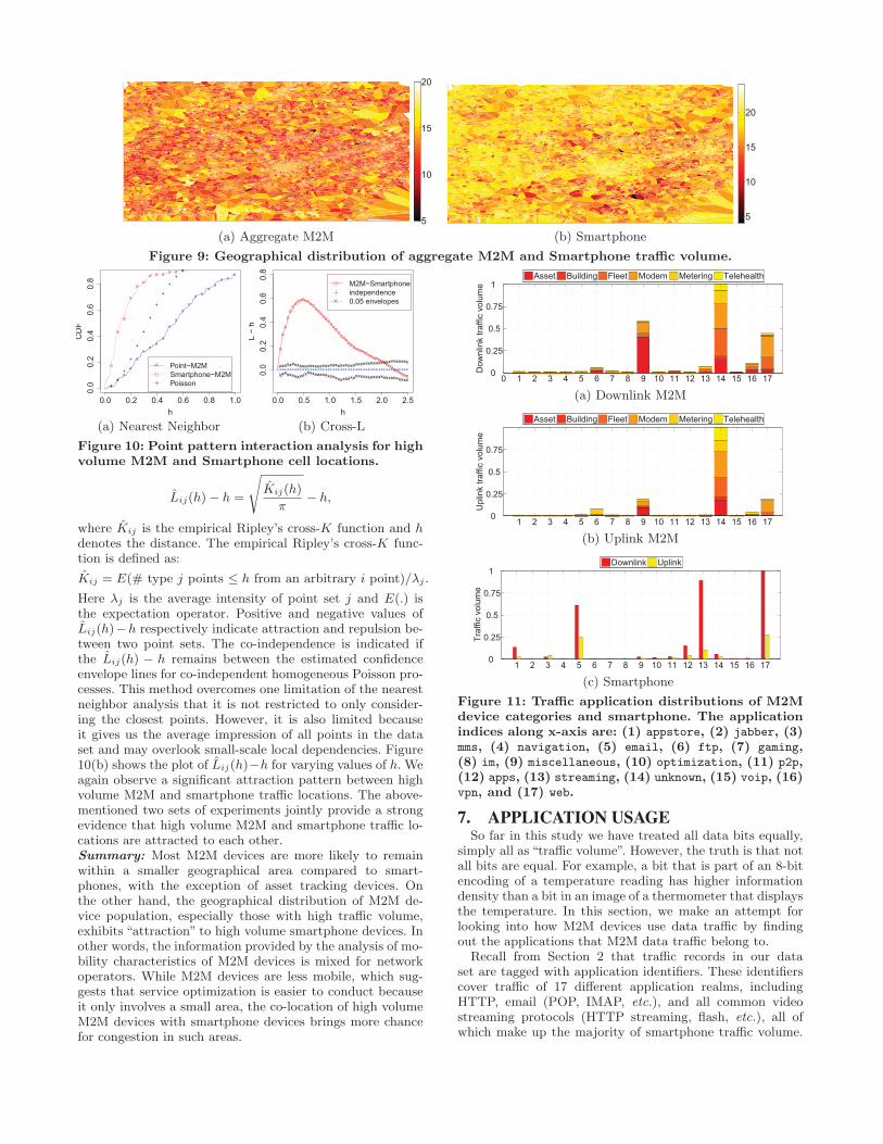
5

10

15

20

(a) Aggregate M2M

5

10

15

20

(b) Smartphone

Figure 9: Geographical distribution of aggregate M2M and Smartphone traffic volume.

xx

xx

xx

xx

x

xx

xx

x xx

xx x

x

0.0 0.2 0.4 0.6 0.8 1.0

0.0

0.2

0.4

0.6

0.8

h

CD

F

o

o

o

o

oo

o o o o o o

++

+

+

+

+

+

+

+

++

+

Point−M2MSmartphone−M2MPoisson

(a) Nearest Neighbor

o

oo

oooooooooooooooooooo

oooooooooooooooooooooooooooo

0.0 0.5 1.0 1.5 2.0 2.5

0.0

0.2

0.4

0.6

0.8

h

L −

h

xxxxxxxxxxxxxxxxxxxxxxxxxxxxxxxxxxxxxxxxxxxxxxxxxxx

xxxxxxxxxxxxxxxxxxxxxxxxxxxxxxxxxxxxxxxxxxxxxxxxxxx

+++++++++++++++++++++++++++++++++++++++++++++++++++

M2M−Smartphoneindependence0.05 envelopes

(b) Cross-L

Figure 10: Point pattern interaction analysis for highvolume M2M and Smartphone cell locations.

L̂ij(h)− h =

√K̂ij(h)

π− h,

where K̂ij is the empirical Ripley’s cross-K function and hdenotes the distance. The empirical Ripley’s cross-K func-tion is defined as:

K̂ij = E(# type j points ≤ h from an arbitrary i point)/λj .

Here λj is the average intensity of point set j and E(.) isthe expectation operator. Positive and negative values ofL̂ij(h)−h respectively indicate attraction and repulsion be-tween two point sets. The co-independence is indicated ifthe L̂ij(h) − h remains between the estimated confidenceenvelope lines for co-independent homogeneous Poisson pro-cesses. This method overcomes one limitation of the nearestneighbor analysis that it is not restricted to only consider-ing the closest points. However, it is also limited becauseit gives us the average impression of all points in the dataset and may overlook small-scale local dependencies. Figure10(b) shows the plot of L̂ij(h)−h for varying values of h. Weagain observe a significant attraction pattern between highvolume M2M and smartphone traffic locations. The above-mentioned two sets of experiments jointly provide a strongevidence that high volume M2M and smartphone traffic lo-cations are attracted to each other.Summary: Most M2M devices are more likely to remainwithin a smaller geographical area compared to smart-phones, with the exception of asset tracking devices. Onthe other hand, the geographical distribution of M2M de-vice population, especially those with high traffic volume,exhibits “attraction” to high volume smartphone devices. Inother words, the information provided by the analysis of mo-bility characteristics of M2M devices is mixed for networkoperators. While M2M devices are less mobile, which sug-gests that service optimization is easier to conduct becauseit only involves a small area, the co-location of high volumeM2M devices with smartphone devices brings more chancefor congestion in such areas.

Dow

nlin

k tra

ffic

volu

me

0 1 2 3 4 5 6 7 8 9 10 11 12 13 14 15 16 170

0.25

0.5

0.75

1Asset Building Fleet Modem Metering Telehealth

(a) Downlink M2M

Upl

ink

traffi

c vo

lum

e

1 2 3 4 5 6 7 8 9 10 11 12 13 14 15 16 170

0.25

0.5

0.75

Asset Building Fleet Modem Metering Telehealth

(b) Uplink M2M

1 2 3 4 5 6 7 8 9 10 11 12 13 14 15 16 170

0.25

0.5

0.75

1

Traf

fic v

olum

e

Downlink Uplink

(c) Smartphone

Figure 11: Traffic application distributions of M2Mdevice categories and smartphone. The applicationindices along x-axis are: (1) appstore, (2) jabber, (3)mms, (4) navigation, (5) email, (6) ftp, (7) gaming,(8) im, (9) miscellaneous, (10) optimization, (11) p2p,(12) apps, (13) streaming, (14) unknown, (15) voip, (16)vpn, and (17) web.

7. APPLICATION USAGESo far in this study we have treated all data bits equally,

simply all as “traffic volume”. However, the truth is that notall bits are equal. For example, a bit that is part of an 8-bitencoding of a temperature reading has higher informationdensity than a bit in an image of a thermometer that displaysthe temperature. In this section, we make an attempt forlooking into how M2M devices use data traffic by findingout the applications that M2M data traffic belong to.

Recall from Section 2 that traffic records in our dataset are tagged with application identifiers. These identifierscover traffic of 17 different application realms, includingHTTP, email (POP, IMAP, etc.), and all common videostreaming protocols (HTTP streaming, flash, etc.), all ofwhich make up the majority of smartphone traffic volume.

Using this application classification, we can compute appli-cation distribution of traffic volume for M2M device cate-gories. We observe that most of the flows, up to 95%, in ourlogged trace use TCP. This observation is in accordance withthe findings reported in prior literature [12,16]. We providethe averaged uplink and downlink application distributionof traffic volume for M2M device categories in Figure 11. Tofirst average a device category, we take the ratio of the sum oftraffic volume of all devices and the total number of devices.We then normalize the averaged traffic application volumesby their maximum value. Figures 11(a) and (b) show thatthe traffic of all device categories mostly belongs to unknownor miscellaneous realms. This indicates that M2M devicestypically use custom protocols that are either not identifiedby our application classification methodology, mentioned inSection 2, or they use atypical protocols.

It is interesting to compare application distribution ofM2M traffic with that of smartphone traffic shown in Fig-ure 11(c). As expected, smartphone traffic mostly belongsto web browsing, audio and video streaming, and email ap-plications. This is in sharp contrast to what we have ob-served for M2M traffic. Another interesting aspect for Fig-ure 11 is that M2M traffic has approximately similar uplinkand downlink traffic volume for most categories and applica-tions while smartphones have more downlink traffic volumethan uplink traffic volume across all applications. This re-sult echoes what we discovered in Sections 3 and 4, yet withdetails along one more dimension – applications.Summary: M2M devices mostly use non-standard applica-tion protocols. This makes it more difficult for network op-erators to mitigate adverse effects from these protocols com-pared to the standard ones such as HTTP. Towards this end,better standardization of M2M protocols would certainly bea mutually beneficial solution for both M2M application ser-vice providers and cellular network operators.

8. NETWORK PERFORMANCEWe now characterize the network performance of M2M

traffic. We examine network performance in terms of roundtrip time (RTT) and packet loss ratio, both of which provideus unique perspectives of network performance.Round Trip Time: RTT is an important metric for net-work performance evaluation and is a key performance in-dicator that quantifies delay in cellular networks. The RTTmetric is especially important for M2M applications thatare real-time critical. It is important to note that RTTmeasurements can be potentially biased by differences inthe paths between different cellular devices and the exter-nal servers they communicate with. For this study, we onlyhave RTT measurements for TCP flows, which are estimatedby the time duration between the trace collecting appara-tus seeing a SYN packet and its corresponding ACK packetin the TCP handshake. Figure 12(a) shows the CDFs ofthe median RTTs experienced by each device for smart-phones and all M2M device categories. We observe that allM2M device categories experience larger RTT compared tosmartphones. Furthermore, within M2M device categories,telehealth devices have smaller RTT than all other cate-gories. Our manual investigation of hardware specificationsshowed that smartphones and telehealth devices are mostlyequipped with 3G modems, in contrast to other categoriesthat typically rely on 2G modems. 2G RTTs are larger dueto longer delays on the air interface, which explains theseobservations.

0.25 0.5 0.75 1 20

0.2

0.4

0.6

0.8

1

CD

F

Median RTT (sec)

SmartphoneM2MAssetBuildingFleetModemMeteringTelehealth

(a) Round trip time

0.025 0.05 0.075 0.1 0.2 0.3 0.4 0.50

0.2

0.4

0.6

0.8

1

Packet Loss Ratio

CD

F

SmartphoneM2MAssetBuildingFleetModemMeteringTelehealth

(b) Packet loss ratio

Figure 12: CDFs of round trip time and packet lossratio.Packet Loss Ratio: Packet loss ratio is a key perfor-mance indicator metric that quantifies reliability in cellu-lar networks. We estimate the packet loss ratio as the ratioof observed TCP payload bytes to the observed TCP se-quence number range, summed over all TCP flows. Sincemost packet loss occurs in the radio access network (RAN)and our measurement point is in between the RAN andthe Internet, this metric effectively estimates the downlinkpacket loss ratio. Figure 12(b) shows the CDFs of packetloss ratio for smartphones and all M2M device categories.Similar to the CDFs of RTT shown in Figure 12(a), we ob-serve differences for packet loss ratio distribution in termsof third and fourth quartile values, where smartphones andtelehealth devices experience at least an order of magnitudelower loss ratios than other M2M device categories due toa larger ratio of 3G to 2G modems. We also observe thatbuilding security devices have much higher third and fourthquartile loss ratios than other M2M devices, despite usingsimilar technologies. This may be due to the placement ofthese devices indoors where the signal quality is poorer.Summary: M2M traffic’s network performance also differsfrom that of smartphones. The RTT of M2M traffic is sig-nificantly larger than smartphone traffic. Careful inspectionof the hardware specifications of M2M devices reveals thatM2M devices generally fall behind smartphones in choiceof cellular technology. A majority of M2M devices still use2G technologies such as GPRS and EDGE. Although 2Gtechnologies are often adequate for M2M communication interms of data rates, such lagging does present a challenge forcellular operators because they would need to maintain oldergeneration services, instead of repurposing 2G spectrum fornewer technologies of higher spectral efficiency. M2M trafficalso generally has higher packet loss ratios. This is proba-bly due to poor deployment location choices for which thelikely reasons are application specific location requirementsor the lack of user interface that clearly displays cellularsignal strength.

9. RELATED WORKTo our best knowledge, this paper presents the first study

on characterizing M2M traffic patterns. Prior related workonly focuses on characterizing general Internet traffic in cel-

lular networks. Due to lack of space, we briefly describe onlyprominent related work below.

General Smartphone Usage: Falaki et al. conducted ameasurement study of smartphone usage [11]. They collecteddata from smartphones of 255 users with only Android andWindows Mobile platforms. The results of their experimen-tal studies indicate significant diversity among smartphoneusage of different users. In contrast to this work on smart-phone activities, our work focuses on M2M data traffic anal-ysis as seen by the cellular network. Furthermore, the scaleof our study, in terms of the number of unique device models,is several orders of magnitude larger.

Smartphone Apps: In [24], Xu et al. characterized usagepatterns of smartphone apps in a 3G cellular network. Theyobserved that different types of apps had different diurnaland mobility patterns. Similarly, we observe different diur-nal and mobility patterns for different M2M device models.In contrast to their study, we find that most M2M appli-cations use custom protocols that are not identifiable usingthe traffic classification technique used in [24]. Thus, M2Mtraffic is a disjoint set of traffic from smartphone app traffic.

Cellular Devices: In [18], Shafiq et al. studied the tem-poral dynamics and distribution of applications in Internettraffic of cellular devices. The authors only studied charac-teristics of 3 cellular device families in their measurementanalysis, whereas we study characteristics of more than 150M2M device models. Furthermore, we additionally exploreInternet traffic dynamics of M2M devices along the dimen-sions of mobility, network performance, and session-levelanalysis.

Mobility and Network Performance: In another re-cent related work, Tso et al. evaluated network performanceof users in different mobility scenarios in a cellular net-work [22]. They collected network performance data for 4laptops, 4 modems, and 4 smartphones. Similar to our anal-ysis, they also studied the network performance metrics suchas round trip time and loss rate. In contrast to this workon network performance in different mobility scenarios, ourwork focuses on large scale characterization of traffic frommore than 150 M2M device models.

10. CONCLUSIONSThis paper presents the first attempt to characterize M2M

traffic in cellular data networks. Our study was based on aweek long traffic trace collected from a major cellular serviceprovider’s core network in the United States. In our analy-sis, we compared M2M and smartphone traffic in severalaspects including temporal traffic patterns, device mobil-ity, application usage, and network performance. We foundthat although M2M devices have different traffic patternsfrom smartphones, they are generally competing with smart-phones for shared network resources. Our findings presentedin this paper have important implications on cellular net-work design, management, and optimization. Through bet-ter understanding of M2M traffic, cellular service providerscan improve resource allocation mechanisms and developbetter billing strategies for different categories of M2M de-vices. The methodology developed in this paper for M2Mtraffic analysis is generic and can also be deployed for moregeneral cellular traffic analyses.

AcknowledgementsWe thank our shepherd, Anirban Mahanti, and the anony-mous reviewers for their useful feedback on this paper.

11. REFERENCES[1] AT&T specialty vertical devices.

www.rfwel.com/support/hw-support/ATT SpecialtyVerticalDevices.pdf.

[2] Evolved Cellular Network Planning and Optimization forUMTS and LTE.

[3] 3G machine-to-machine (M2M) communications: Cellular3G, WiMAX, and municipal Wi-Fi for M2M applications.Technical report, ABIresearch, 2007.

[4] The global wireless M2M market. Technical report, BergInsight, December 2010.

[5] Cisco visual networking index: Global mobile data trafficforecast update, 2011-2016. White Paper, 2012.

[6] R. S. Bivand, E. J. Pebesma, and V. Gomez-Rubio. AppliedSpatial Data Analysis with R. Springer, 2008.

[7] CalAmp. LMU-2600 GPRS fleet tracking unit.http://www.calamp.com/ pdf/LMU-2600.pdf.

[8] P. Chaovalit, A. Gangopadhyay, G. Karabatis, and Z. Chen.Discrete wavelet transform-based time series analysis andmining. ACM Computing Surveys, 43(2), 2011.

[9] J. Erman, A. Gerber, M. T. Hajiaghayi, D. Pei, andO. Spatscheck. Network-aware forward caching. In WWW,2009.

[10] Z. M. Fadlullah, M. M. Fouda, N. K. A. Takeuchi,N. Iwasaki, and Y. Nozaki. Toward intelligentmachine-to-machine communications in smart grid. IEEECommunications Magazine, 49(4):60–65, 2011.

[11] H. Falaki, R. Mahajan, S. Kandula, D. Lymberopoulos,R. Govindan, and D. Estrin. Diversity in smartphoneusage. In MobiSys, 2010.

[12] A. Gerber, J. Pang, O. Spatscheck, and S. Venkataraman.Speed testing without speed tests: Estimating achievabledownload speed from passive measurements. In ACM IMC,2010.

[13] N. Grira, M. Crucianu, and N. Boujemaa. Unsupervisedand semi-supervised clustering: A brief survey. Report ofthe MUSCLE European Network of Excellence (FP6), 2004.

[14] L. K. Law, S. V. Krishnamurthy, and M. Faloutsos.Capacity of hybrid cellular-ad hoc data networks. InINFOCOM, 2008.

[15] Z. Moczar and S. Molnar. Comparative traffic analysisstudy of popular applications. In International Conferenceon Energy-aware Communications, 2011.

[16] U. Paul, A. P. Subramanian, M. M. Buddhikot, and S. R.Das. Understanding traffic dynamics in cellular datanetworks. In INFOCOM, 2011.

[17] F. Qian, Z. Wang, A. Gerber, Z. M. Mao, S. Sen, andO. Spatscheck. Characterizing radio resource allocation for3G networks. In ACM IMC, 2010.

[18] M. Z. Shafiq, L. Ji, A. X. Liu, and J. Wang. Characterizingand modeling Internet traffic dynamics of cellular devices.In ACM SIGMETRICS, 2011.

[19] P. Stoica and R. L. Moses. Introduction to SpectralAnalysis. Prentice Hall, 1997.

[20] P. Traynor, M. Lin, M. Ongtang, V. Rao, T. Jaeger,P. McDaniel, and T. L. Porta. On cellular botnets:measuring the impact of malicious devices on a cellularnetwork core. In ACM CCS, 2009.

[21] Trilliant. CellReader digital cellular meters.http://www.trilliantinc.com/ products/cellreader/.

[22] F. P. Tso, J. Teng, W. Jia, and D. Xuan. Mobility: Adouble-edged sword for HSPA networks. In MobiHoc, 2010.

[23] I. T. Union. World telecommunication/ICT indicatorsdatabase 2011. http://www.itu.int/ITU-D/ict/publications/world/world.html, 2011.

[24] Q. Xu, J. Erman, A. Gerber, Z. M. Mao, J. Pang, andS. Venkataraman. Identifying diverse usage behaviors ofsmartphone apps. In ACM IMC, 2011.

[25] Q. Xu, A. Gerber, Z. M. Mao, and J. Pang. AccuLoc:Practical localization of peformance measurement in 3Gnetworks. In ACM MobiSys, 2011.